Closing the Plio-Pleistocene ¹³C cycle in the 405 kyr periodicity by isotopic signatures of geological sources

The ¹³C cycle of the Plio-Pleistocene, as recorded in δ¹³C of benthic foraminifera, has power in periodicities related to the long eccentricity cycle of 405 kyr that is missing in corresponding climate records (e.g. δ¹⁸O). Using a global carbon cycle model, I show in an inverse approach that the long eccentricity in δ¹³C might have been caused by variations in the isotopic signature of geological sources, namely of the weathered carbonate rock (δ¹³C_rock) or of volcanically released CO₂ (δ¹³C_v). This closure of the ¹³C cycle in these periodicities also explains the offset in atmospheric δ¹³CO₂ seen between the Penultimate Glacial Maximum (PGM) and the Last Glacial Maximum (LGM). The necessary isotopic signatures in δ¹³C_rock or δ¹³C_v, which align my simulations with reconstructions of the ¹³C cycle on orbital timescales, have the most power in the obliquity band (41 kyr), suggesting that land ice dynamics are the ultimate cause for these suggested variations. Since the Asian monsoon as reconstructed from speleothems also has an obliquity-related component and since precipitation (or runoff) is one main driver for local weathering rates, it is possible that these proposed changes in weathering are indeed, at least partly, connected to the monsoon as previously suggested. Alternatively, the suggested impact of land ice or sea level on volcanic activity might also be influential for the ¹³C cycle. This indirect influence of ice sheets on the long eccentricity cycle in δ¹³C implies that these processes might not have been responsible for the 405 kyr periodicity found in times of the pre-Pliocene parts of the Cenozoic that have been largely ice-free in the Northern Hemisphere.

1 Introduction

The long eccentricity cycle with a periodicity of 405 kyr is missing in most climate signals for the last 5 Myr, e.g. in the benthic δ¹⁸O (Lisiecki and Raymo, 2005), but is imprinted on the global carbon cycle, since significant power in it is contained in benthic δ¹³C (e.g. Mix et al., 1995b; Wang et al., 2010). For earlier parts of the Cenozoic, the 405 kyr cycle is not only found in δ¹³C but also in δ¹⁸O (Pälike et al., 2006; Zeebe et al., 2017; De Vleeschouwer et al., 2020; Westerhold et al., 2020). This difference between climate and carbon cycle makes the interpretation of the Plio-Pleistocene ¹³C cycle, and related interpretations with respect to processes responsible for changes in atmospheric CO₂, challenging.

Some interpretations of the impact of long eccentricity on δ¹³C have been put forward. Russon et al. (2010) used a carbon cycle box model to analyse how oceanic processes, e.g. small changes in nutrient availability or in the ratio of organic matter to CaCO₃ in the export production, might have caused these δ¹³C changes. They already point out that changes in only the ¹³C cycle but not in atmospheric CO₂, and therefore global climate, are difficult to explain. Ma et al. (2011) used a slightly different box model and proposed that eccentricity impacts on the weathering intensity and nutrient supply ultimately changed δ¹³C in ∼ 400 kyr periodicity during the Miocene. Paillard (2017) used a conceptual model and suggested that riverine organic carbon inputs into the ocean caused by sea-level-related erosion at river mouths might be responsible for ∼ 400 kyr variability in δ¹³C of the last 4 Ma. In a data review, Wang et al. (2014) also proposed that the origin of this low δ¹³C frequency is related to riverine input but suggested that the underlying process is the monsoon intensity.

While the long-term changes in δ¹³C in the ocean have long been known (e.g. Mix et al., 1995b), the record of δ¹³CO₂ from ice cores is still relatively new and, at 155 kyr, rather short (Eggleston et al., 2016). New ice core data across Termination IV (around 340 kyr BP) offer another ∼ 10 kyr long snapshot of changes in δ¹³CO₂ (Krauss et al., 2025). When δ¹³CO₂ data across Termination II were first measured (Schneider et al., 2013), an apparent offset between the Penultimate Glacial Maximum and the Last Glacial Maximum (PGM and LGM, respectively) of +0.45 ‰ prevented a straightforward interpretation of the data. Among other possibilities, the authors speculated that geological processes, namely changes in the isotopic ratio of carbonate weathering or in the contributions from volcanic input fluxes, might explain this offset in δ¹³CO₂. However, it had not yet been discussed in the ice core community (Schneider et al., 2013; Eggleston et al., 2016) if the PGM-to-LGM offset in δ¹³CO₂ and the long eccentricity cycle in benthic δ¹³C were related to each other.

Here, I use the well-established global carbon cycle box model BICYCLE-SE (Köhler and Munhoven, 2020) to test in detail if these geological processes proposed by Schneider et al. (2013) might indeed be responsible for the PGM-to-LGM offset in δ¹³CO₂ and eventually also for the changes in the ¹³C cycle related to the long eccentricity. For that effort, I first reanalyse previously published simulations which were performed with an updated ¹³C cycle over the time window covered by δ¹³CO₂ (Köhler and Mulitza, 2024). In that study, atmospheric δ¹³CO₂ was already prescribed by the ice core data in some simulations and not internally calculated in the model. This approach indirectly introduced some long-term variability in δ¹³C to the whole ¹³C cycle, while the boundary conditions changing the main carbon cycle and CO₂ were not modified. I first analyse if and how these changes in ¹³C necessary for δ¹³CO₂ to agree with ice core reconstructions might have been caused by the two geological processes of interest. I then add further scenarios to my assessment, in which one variable of the ¹³C cycle in the model is not prescribed by data but only weakly nudged to a δ¹³C time series. This nudging approach reduces the amount of necessary adjustments considerably and is first applied to atmospheric δ¹³CO₂ and then expanded to deep-ocean δ¹³C in order to be able to cover simulations longer than 155 kyr. Building on earlier work, I then extend my investigation to simulations covering the ice core time window of the last 800 kyr (Köhler and Munhoven, 2020) and finally the last 5 Myr covering most of the Plio-Pleistocene (Köhler, 2023). Such an approach of nudging the model to data is an inverse investigation, which offers new insights not directly (or only with a time-consuming effort) available from classical forward modelling. While in the latter well-defined hypotheses are tested by changing the boundary conditions or processes beforehand in simulated scenarios, the inverse approach offers solutions one might not have been looking for (e.g. unexpected frequencies in the variables of investigation). As a side effect, my nudging approach might also increase the simulated glacial–interglacial (G-IG) amplitudes in δ¹³C in the earlier parts of the Plio-Pleistocene and bring them in better agreement with reconstructions (Köhler and Bintanja, 2008).

2 Methods

2.1 Data

To perform this analysis, the following data (reconstruction) are needed: Plio-Pleistocene deep-ocean time series of benthic δ¹³C and δ¹⁸O, all available atmospheric δ¹³CO₂ from ice cores and Late Pleistocene surface-ocean (planktic) δ¹³C, and estimates on the variability in the δ¹³C signature from carbonate rock weathering and volcanic CO₂ outgassing. These data are described in detail in this subsection.

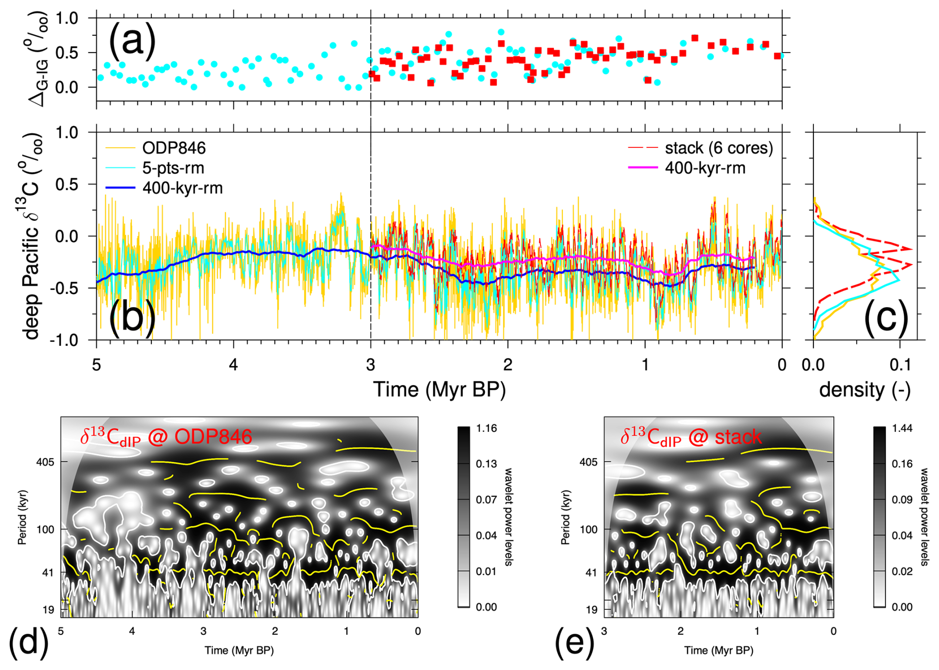
Figure 1 Deep Pacific Plio-Pleistocene δ¹³C data based on either ODP846 (Mix et al., 1995a; Shackleton et al., 1995; Poore et al., 2006) or a stack from six cores (Lisiecki, 2014). The temporal resolution is 1 kyr in the stack and partly up to 2 kyr in ODP846, and these values are interpolated to an equidistant 1 kyr for further analysis. (a) G-IG amplitudes of records shown in panel (b). Here, the difference between a glacial minimum and the subsequent interglacial maximum is calculated following the MIS boundary definition of Lisiecki and Raymo (2005), with points being positioned at mid-transitions. (b) Time series. The 400 kyr running means and a five-point running mean of ODP846 are added to improve comparison to the stack. The vertical line at 3 Myr BP marks the start point of the records for the analysis shown in panel (c). (c) Normalised data density distribution of the last 3 Myr of the δ¹³C time series shown in panel (b). (d) Wavelet of the 5 Myr long five-point running mean of δ¹³C from ODP846. (e) Wavelet of the 3 Myr long deep Pacific δ¹³C stack.

2.1.1 Plio-Pleistocene deep-ocean time series

Due to the large volume of the Pacific Ocean, whole-ocean changes in δ¹³C are approximated to a first order with benthic δ¹³C data from the deep Pacific. Under this premise, a deep Pacific δ¹³C stack consisting of six sediment cores (Lisiecki, 2014) illustrates the variability in oceanic δ¹³C over the last 3 Myr (Fig. 1b), which is in its long-term variability, but with higher short-term scatter and a lower long-term mean by 0.1 ‰, nicely matched by δ¹³C from ODP846 (Mix et al., 1995a; Shackleton et al., 1995), which is also one of the cores contributing to the stack. This core, ODP846 (3307 m water depth, 91° W close to the Equator), extends further back in time and is used here as published in Poore et al. (2006) in order to cover a 5 Myr long time window (Fig. 1b).

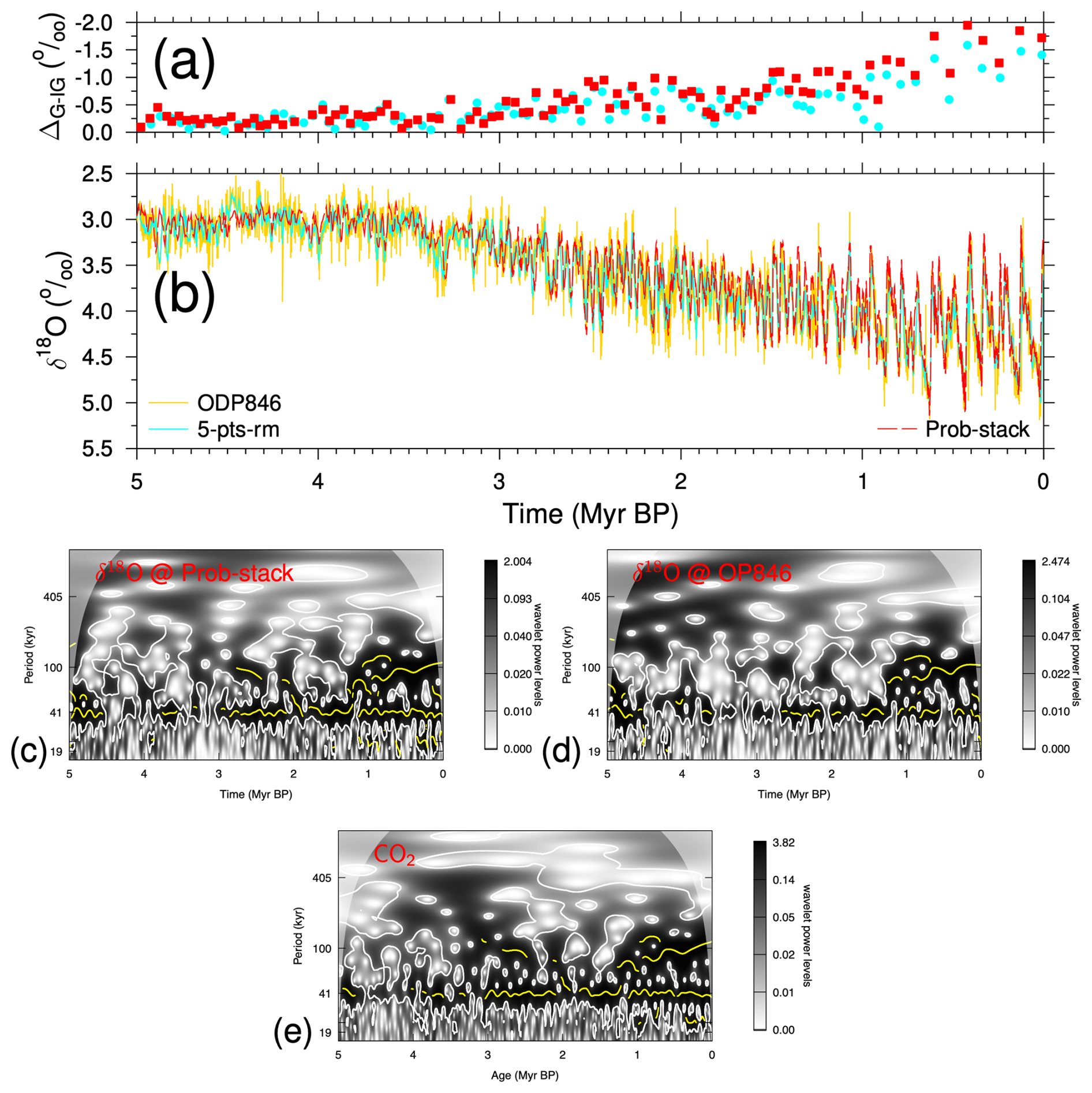
Figure 2 Climate change. (a) Glacial–interglacial amplitudes of records shown in panel (b). Here, the difference between a glacial minimum and the subsequent interglacial maximum is calculated following the MIS boundary definition of Lisiecki and Raymo (2005). Points are positions at the mid-transitions. (b) Benthic δ¹⁸O from ODP846 (Mix et al., 1995a; Shackleton et al., 1995; Poore et al., 2006) and Prob-stack (Ahn et al., 2017). Wavelets of detrended benthic δ¹⁸O from (c) Prob-stack and (d) ODP846 and (e) of simulated atmospheric CO₂ (scenario SEi++V6).

The stacking of cores always introduces a smoothing effect. Therefore, the width of the data distribution of both time series converges (σ≈0.20 ‰) if a five-point running mean is applied to the ODP846 data (Fig. 1c), which in its raw data is more widely distributed (σ=0.26 ‰). Both deep Pacific δ¹³C time series contain significant power in periods longer than 100 kyr in their wavelets (Fig. 1d, e), not only around 405 kyr (∼ 500 kyr in the last 1 Myr), but also in between the eccentricity bands (∼ 200 kyr periodicities). While the latter variability is not known from orbital forcing, it has already been detected in terrestrial sediments of the early Paleocene and might be a sub-harmonic of the 405 kyr periodicity (Hilgen et al., 2020). Alternatively, this power might be related to the 173 kyr periodicity, an amplitude modulation of the 41 kyr of obliquity, which is also found in the Miocene–Pliocene of the Asian monsoon (Zhang et al., 2022) and in total organic carbon during the Mesozoic and Cenozoic (Huang et al., 2021). Power in periodicity between 100 and 405 kyr during the last 5 Myr is also contained in previous wavelet analysis of so-called benthic δ¹³C mega-splices, but it has never been discussed in more detail (De Vleeschouwer et al., 2020; Westerhold et al., 2020).

Spectral analyses of various climate variables find few of these slow changes during the Plio-Pleistocene. Prob-stack (Ahn et al., 2017), the successor to the LR04 benthic δ¹⁸O stack (Lisiecki and Raymo, 2005) based on 180 instead of 57 records, contains little power in 405 kyr periodicity during the last 2.5 Myr but some power earlier on (Fig. 2b, c), similarly to δ¹⁸O in ODP846, the deep Pacific core containing the δ¹³C used here (Mix et al., 1995a; Shackleton et al., 1995; Poore et al., 2006) (Fig. 2b, d). This long eccentricity cycle is also missing in the last 2.5 Myr and is only weakly contained earlier in time series of my simulated atmospheric CO₂ (Fig. 2e). For the interpretation of the rather unusual frequencies around 200 kyr in δ¹³C and the absence of the long eccentricity in δ¹⁸O, one should keep in mind that the response of a nonlinear system might exhibit frequencies not present in the original driven forcing (e.g. Rial, 1999; Rial et al., 2004).

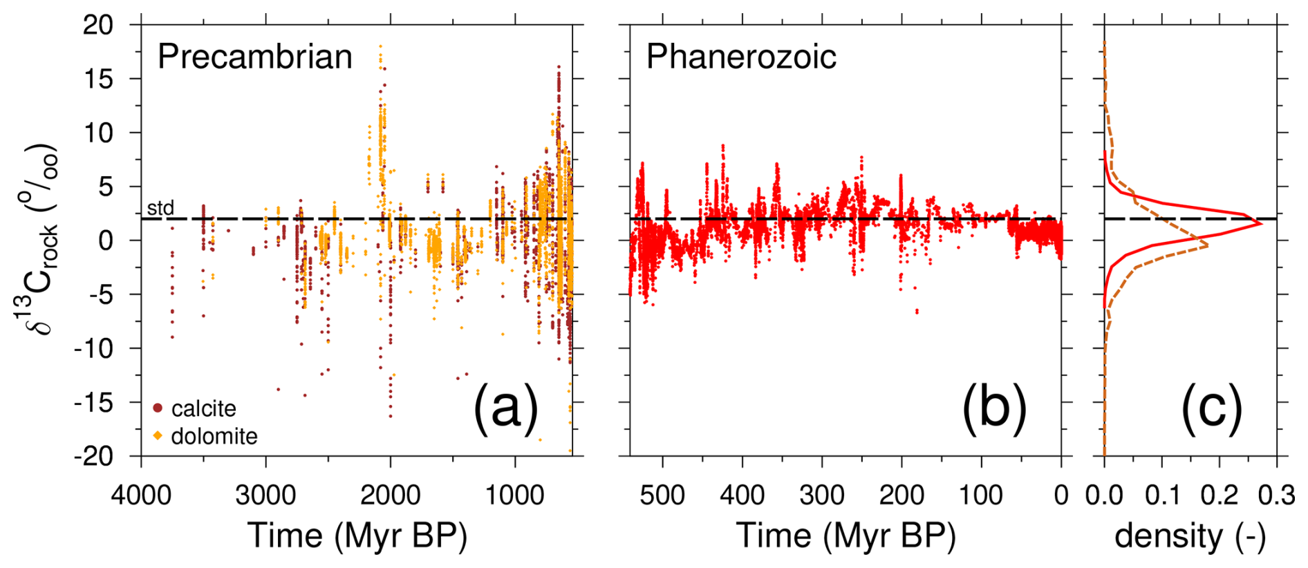
Figure 3 The δ¹³C from carbonate rock from Earth's history. (a) Precambrian values of δ¹³C calcite and dolomite rock as compiled in Prokoph et al. (2008). (b) Phanerozoic values as compiled in Bachan et al. (2017). (c) Normalised density plot of δ¹³C data (broken line: Precambrian; solid line: Phanerozoic). The standard (std) parameter value of δ¹³C_rock=2.0 ‰ used in the BICYCLE-SE model is also marked.

Furthermore, during the Mid-Pleistocene Transition (MPT) around 1 Ma, climate changed from a dominantly 41 kyr periodicity during the Pliocene and Early Pleistocene to a 100 kyr periodicity on average in the Late Pleistocene (e.g. Shackleton and Opdyke, 1976; Pisias and Moore-Jr., 1981). Since there is hardly any change in incoming solar radiation with power in the 100 kyr band (Laskar et al., 2004), this MPT is still not completely understood, but it has so far been hypothesised to have been caused by non-linear processes in the carbon cycle–climate system (e.g. Willeit et al., 2019; Berends et al., 2021; Clark et al., 2024). An accompanying feature of the MPT is the rise in G-IG amplitudes, as, for example, seen in benthic δ¹⁸O (Lisiecki and Raymo, 2005; Ahn et al., 2017) or in global temperature compilations (Clark et al., 2024). Benthic δ¹³C also includes this transition in power from 41 kyr to 100 kyr frequency across the MPT (e.g. Köhler and Bintanja, 2008). However, G-IG amplitudes in benthic δ¹³C only gradually increase over the Plio-Pleistocene. In both the deep Pacific core ODP846 or the deep Pacific stack in the 41 kyr world, the size of these amplitudes is on average 68 %–76 % of their mean amplitude found in the 100 kyr world of the last 1 Myr (Fig. 1a). This is markedly different from benthic δ¹⁸O, whose G-IG amplitudes in the 41 kyr world have been on average only 35 %–39 % of their size during the last 1 Myr (Fig. 2a).

These two aspects, long eccentricity cycle and G-IG amplitudes, in which δ¹³C differs from climate variables during the Plio-Pleistocene, suggest that the carbon cycle and the climate system are partly decoupled on orbital timescales.

2.1.2 Late Pleistocene surface-ocean δ¹³C and atmospheric δ¹³CO₂

The continuous 155 kyr long time series of atmospheric δ¹³CO₂ (Eggleston et al., 2016) has been shown to be highly correlated, especially on orbital timescales, to two monospecific stacks of δ¹³C from planktic foraminifera from latitudes <40°, also called wider tropics (Köhler and Mulitza, 2024). This latter study could not identify any impact of the so-called carbonate ion effect proposed from laboratory experiments (Spero et al., 1997), which is why the planktic δ¹³C stacks can be regarded as reliable recorders of δ¹³C in dissolved inorganic carbon (δ¹³C_DIC) in the surface ocean of the wider tropics. Underlying data were compiled from sediments cores at latitudes <40°, roughly in agreement with the non-polar (sometimes called equatorial) surface-ocean boxes in the model. To my knowledge, there exists no robust longer time series of planktic δ¹³C. Due to the shortness of these time series, a spectral analysis with focus on the long eccentricity cycle is not possible. However, these data might be helpful in a comparison with simulation results. Recently, another ∼ 10 kyr long part of δ¹³CO₂ across Termination IV was published (Krauss et al., 2025).

2.1.3 The δ¹³C signature of the geological source of carbonate weathering

Present-day mountains were built during the Phanerozoic (the last 540 Myr), but there are also various areas with Precambrian shields (older than 540 Myr), e.g. in North America (e.g. Whitmeyer and Karlstrom, 2007; Faccenna et al., 2021). It is thus worth considering how δ¹³C in carbonate rocks (δ¹³C_rock) changed over these time spans. The records of δ¹³C in carbonates during the Phanerozoic (Fig. 3b) have varied for most of the last 440 Myr between 0 ‰ and +5 ‰, with short-term excursions up to +8 ‰ and −5 ‰ (Bachan et al., 2017). The earliest part of the Phanerozoic (440–540 Myr) covering the Cambrian and the Ordovician generally contained lower values (−5 ‰ to 0 ‰), with peaks up to +7 ‰ (Bachan et al., 2017). A compilation of raw whole-rock δ¹³C isotope data for limestone and dolomite for the Precambrian (Fig. 3a) contains a huge scatter from −10 ‰ to +10 ‰, with a few excursions up to ±20 ‰ (Prokoph et al., 2008).

Calculated density distributions of these time series of δ¹³C_rock (Fig. 3c) are nearly normally distributed for the Phanerozoic, with the mode being slightly lower (mean $\pm \mathit{\sigma }=+\mathrm{1.5}\pm \mathrm{1.6}$ ‰) than the chosen standard parameter values of ${\mathit{\delta }}^{\mathrm{13}}{\mathrm{C}}_{\mathrm{rock}}=+\mathrm{2}\mathrm{‰}$ in the BICYCLE-SE model (see Sect. 2.2.1). Here, data are interpolated to 10-year equidistant values before analysis. Data from the Precambrian have much larger gaps than for the Phanerozoic, which is why interpolation is not applied. The distribution of the Precambrian δ¹³C_rock, combining both calcite and dolomite, is wider than for the Phanerozoic, with a small mean value ($+\mathrm{0.7}\pm \mathrm{3.6}$ ‰).

2.1.4 The δ¹³C signature of volcanic CO₂

In BICYCLE-SE, a δ¹³C of −5 ‰ of volcanic CO₂ emissions (δ¹³C_v) is assumed, agreeing with a typical endmember value from mantle material (Deines, 2002). However, δ¹³C_v data are only available from modern observations, and their variability in the past is unknown. Mid-ocean ridge basalt (MORB) volcanism contributes about 15 % to the global volcanic CO₂ outgassing rate in the present day (Burton et al., 2013) and contains a range of about −9 ‰ to −4 ‰ in δ¹³C_v (Sano and Williams, 1996). The collected δ¹³C_v values from more than 70 arc volcanoes (Mason et al., 2017) are on average (±1σ) $-\mathrm{4.4}\pm \mathrm{2.6}$ ‰. The δ¹³C_v range in arc volcanoes would narrow significantly to an uncertainty of ±0.5 ‰ if weighted by CO₂ fluxes. However, such a weighting is not well constrained, and CO₂ fluxes of different arc systems might have varied in the past. Newer data on arc volcanism from Baja California (Batista Cruz et al., 2019; Barry et al., 2020), not yet included in the review of Mason et al. (2017), show volcanic CO₂ being more depleted in ¹³C, with δ¹³C_v being as low as −19 ‰. Similarly to MORB, the arc volcanism is also responsible for about 15 % of the annual volcanic CO₂ outgassing (Burton et al., 2013; Mason et al., 2017; Fischer and Aiuppa, 2020). Furthermore, new data on a 2021 volcanic eruption in Iceland (Moussallam et al., 2024) found a ${\mathit{\delta }}^{\mathrm{13}}{\mathrm{C}}_{\mathrm{v}}=\mathrm{0.1}\pm \mathrm{1.2}$ ‰. This is within the range of Icelandic ${\mathit{\delta }}^{\mathrm{13}}{\mathrm{C}}_{\mathrm{v}}\in [-\mathrm{18.8},+\mathrm{4.6}]\mathrm{‰}$ (Barry et al., 2014) but on the upper end of the Gaussian distribution given by the ${\mathit{\delta }}^{\mathrm{13}}{\mathrm{C}}_{\mathrm{v}}=-\mathrm{3.0}\pm \mathrm{2.0}$ ‰ by which the Icelandic compilation of Barry et al. (2014) is condensed in Mason et al. (2017). Indications for temporal variations in δ¹³C_v in individual volcanoes also exist. For example, Chiodini et al. (2011) detected a positive trend in δ¹³C_v for the Etna, rising from −4 ‰ to −1 ‰ within 3–4 decades of the recent past. Altogether, the collected data suggest large heterogeneity of the mantle source, making a temporal fast-changing δ¹³C_v (as suggested here) plausible. However, although δ¹³C_v data from arc volcanism and MORB are reasonably well covered, the related CO₂ fluxes add up to only ∼30 % of the global volcanic outgassing. Thus, a complete picture of the variety of δ¹³C_v including other sources, such as hotspot volcanoes, tectonic degassing, and volcanic lakes (Burton et al., 2013; Fischer and Aiuppa, 2020), is still missing.

2.2 Model

2.2.1 The carbon cycle box model BICYCLE-SE

The carbon cycle box model BICYCLE-SE is fully described in Köhler and Munhoven (2020), and its ¹³C cycle has recently been updated (Köhler and Mulitza, 2024). This model version has recently been used to show that simulated changes in the radiocarbon age of the ocean between the LGM and preindustrial times agree reasonably well with reconstructions, although, on millennial timescales (ignored here), abrupt changes in ocean circulation related to the bipolar seesaw need to be considered to meet deep-ocean ¹⁴C data (Köhler et al., 2024). Briefly, the BICYCLE core of the model consists of 10 ocean boxes, 7 boxes for terrestrial carbon pools, and 1 box for the atmosphere. Carbon and the carbon isotopes (and alkalinity, O₂, and PO${}_{\mathrm{4}}^{\mathrm{3}-}$ in the ocean) are calculated state variables of the model with explicitly considered carbonate chemistry in the ocean that distributes DIC as function of temperature, salinity, and pressure into its three chemical species (CO₂, HCO${}_{\mathrm{3}}^{-}$, CO${}_{\mathrm{3}}^{\mathrm{2}-}$). In its update to a solid Earth (SE) version, the model now contains a process-based sediment module that calculates, depending on carbonate chemistry, either the accumulation or the dissolution of CaCO₃ in the deep ocean and the shallow water loss of CaCO₃ due to coral reef growth, simplistically calculated as a function of chemistry and sea level change. A fixed fraction of 0.6 % of ¹³C-depleted organic matter of the export production of organic carbon that reaches the deep-ocean boxes is permanently buried in the sediment (35×10¹² gC yr⁻¹ in preindustrial times). Thus, organic carbon plays no active role in the sediment module, since its implementation would ask for much more complexity (Munhoven, 2021; Ye et al., 2025), potentially unavailable in box models. The main goal of the sediment module is to mimic the carbonate compensation feedback (Broecker and Peng, 1987), which, according to a model–data comparison of deep-ocean CO${}_{\mathrm{3}}^{\mathrm{2}-}$ data (Yu et al., 2013), is sufficiently obtained (Köhler and Munhoven, 2020). The simulated export of CaCO₃ and organic carbon to the sediment is higher during glacial times than during interglacials by about 50 %, roughly in agreement with reconstructions (Cartapanis et al., 2016, 2018). Furthermore, carbonate and silicate weathering fluxes (on average 12 Tmol yr⁻¹ each) introduce, either constantly or as a function of atmospheric CO₂, a flux of bicarbonate (changing the total amount of both carbon and alkalinity) into the surface ocean. Volcanic CO₂ outgassing on land as a time-delayed function of changing land ice volume, or from island and hotspot volcanoes as a time-delayed function of sea level change (both delayed by 4 kyr; see Kutterolf et al., 2013), are other external carbon sources to the model (about 5–15 Tmol yr⁻¹). More details are found in the earlier papers describing the model.

Isotopic fractionation occurs mainly during gas exchange and biological production on land and in the ocean. The sizes of the corresponding fractionations in the ε notation (in ‰) are summarised in Fig. S1 in the Supplement. Furthermore, the isotopic signatures of the external inputs of carbon in the simulated system – of the weathered carbonate rock (${\mathit{\delta }}^{\mathrm{13}}{\mathrm{C}}_{\mathrm{rock}}=+\mathrm{2}\mathrm{‰}$) and of the volcanic CO₂ (${\mathit{\delta }}^{\mathrm{13}}{\mathrm{C}}_{\mathrm{v}}=-\mathrm{5}\mathrm{‰}$) – are necessary parameters of the model, which so far have been constantly prescribed by the mentioned values.

Climate change (ocean circulation, temperature, sea level and sea ice, aeolian iron input) influencing the marine carbon pumps and land carbon storage is prescribed externally from reconstructions. Here, I use different setups, either covering the 800 kyr long time window with ice core data (Köhler and Munhoven, 2020) or the last 5 Myr with most of the Plio-Pleistocene (Köhler, 2023). Forcing details were described in the relevant studies but are summarised in the Supplement (Figs. S2–S3).

In the model geometry, all of the Indo-Pacific Ocean below 1 km depth is combined in one box called the deep Indo-Pacific. All the relevant deep-ocean δ¹³C data to which I compare my simulation results come from the deep Pacific. I always refer to either of these two elements when talking about the deep (Indo-)Pacific.

2.2.2 Reducing the model–data offset in the ¹³C cycle

Various applications have shown that the model seems to be able to simulate G-IG changes in the carbon cycle in reasonable agreement with various palaeo-data (atmospheric CO₂, deep-ocean CO${}_{\mathrm{3}}^{\mathrm{2}-}$, surface-ocean pH, deep-ocean ¹⁴C) (e.g. Köhler and Munhoven, 2020; Köhler, 2023; Köhler et al., 2024), while the long-term changes in δ¹³C as found in the reconstructions are so far not contained in a satisfactory manner in the model output (e.g. Köhler and Bintanja, 2008; Köhler et al., 2010; Köhler and Mulitza, 2024). Instead of searching for solutions which satisfy equally well the data constraints given by the carbon cycle itself and its stable carbon isotope, I follow a different, inverse approach. I take the main carbon cycle, including simulated atmospheric CO₂ as given, and analyse how changes in the isotopic signatures of the external input of carbon in the simulated system need to vary to align the simulated ¹³C cycle, especially on orbital timescales, with data. In doing so, I come to one possible realisation of how the carbon cycle might have changed in the past, which agrees reasonably well with reconstructions of atmospheric carbon records (CO₂ and δ¹³CO₂) and marine δ¹³C, but I cannot exclude that other solutions might exist. Note that the long-term effect of changes in the weathering flux strength, not its isotopic signature, on the ¹³C cycle has recently been investigated with step changes in the Bern3D model (Jeltsch-Thömmes and Joos, 2023), finding that equilibrium in the ¹³C cycle is only reached after a few hundred thousand years, while that of CO₂ (and of climate) is reached 1 order of magnitude faster.

For that effort, I apply additional constraints to the model. I overwrite (or prescribe) one internally calculated variable of the ¹³C cycle with reconstructions. This would in principle violate mass conservation of ¹³C but not if all necessary changes can be explained by variations in δ¹³C_rock or δ¹³C_v, the isotopic signatures of the geological sources. In a post-processing analysis, I determine their necessary values from model-internal information as described in the following. Initial results already informed me that, when prescribing δ¹³CO₂, the necessary anomalies in isotopic signatures of the external carbon sources need to be a lot larger than the reconstructed ranges. In an alternative approach, I therefore only weakly nudge the simulated δ¹³C variable to its reconstruction. This approach can be used to check on necessary changes in either δ¹³C_rock or δ¹³C_v to align simulations with reconstructions. Both constraints (prescribing or nudging) are applied to either atmospheric δ¹³CO₂ or deep Indo-Pacific δ¹³C. Since my solution is obtained from model–data differences (and not as a hypothesis to be tested that has been put into the model in a transient forward simulation), it can be called an inverse approach. Such inverse approaches typically do not lead to unique solutions but offer new insights that are otherwise not (or hardly) available.

In detail, this approach works as follows: for each year t, the data would require a change Δ(t) (in units of ‰ yr⁻¹) in one variable of the model (δ¹³C_model(t)), e.g.

$$\begin{array}{}\text{(1)}& \mathrm{\Delta }\left(t\right)=\left({\mathit{\delta }}^{\mathrm{13}}{\mathrm{C}}_{\mathrm{data}}\right(t)-{\mathit{\delta }}^{\mathrm{13}}{\mathrm{C}}_{\mathrm{model}}(t\left)\right).\end{array}$$

The difference between this data–model offset Δ(t) and the internally calculated change in this variable $\frac{\mathit{\delta }}{\mathit{\delta }t}\left({\mathit{\delta }}^{\mathrm{13}}{\mathrm{C}}_{\mathrm{model}}^{\mathrm{internal}}\left(t\right)\right)$, weighted by the nudging strength $\mathit{\eta }\in [\mathrm{0},\mathrm{1}]$, is the applied correction Δ_cor(t):

$$\begin{array}{}\text{(2)}& {\mathrm{\Delta }}_{\mathrm{cor}}\left(t\right)=\mathit{\eta }\cdot \left(\mathrm{\Delta }\left(t\right)-{\displaystyle \frac{\mathit{\delta }}{\mathit{\delta }t}}\left({\mathit{\delta }}^{\mathrm{13}}{\mathrm{C}}_{\mathrm{model}}^{\mathrm{internal}}\right(t\left)\right)\right),\end{array}$$

which is added to the differential equation

$$\begin{array}{}\text{(3)}& {\displaystyle \frac{\mathit{\delta }}{\mathit{\delta }t}}\left({\mathit{\delta }}^{\mathrm{13}}{\mathrm{C}}_{\mathrm{model}}^{\mathrm{final}}\left(t\right)\right)={\displaystyle \frac{\mathit{\delta }}{\mathit{\delta }t}}\left({\mathit{\delta }}^{\mathrm{13}}{\mathrm{C}}_{\mathrm{model}}^{\mathrm{internal}}\left(t\right)\right)+{\mathrm{\Delta }}_{\mathrm{cor}}\left(t\right).\end{array}$$

If η=1, these equations simplify to

$$\begin{array}{}\text{(4)}& {\displaystyle \frac{\mathit{\delta }}{\mathit{\delta }t}}\left({\mathit{\delta }}^{\mathrm{13}}{\mathrm{C}}_{\mathrm{model}}^{\mathrm{final}}\left(t\right)\right)=\mathrm{\Delta }\left(t\right),\end{array}$$

and the approach describes the prescription of δ¹³C with data. In other words, prescription is the most extreme case of nudging.

In the post-processing, it is calculated how Δ_cor(t) can be caused by changes in the isotopic signature of the external sources to the simulated carbon cycle. Thus, the following hypothetical isotopic signatures for the external fluxes are calculated:

$$\begin{array}{}\text{(5)}& {\mathit{\delta }}^{\mathrm{13}}{\mathrm{C}}_{\mathrm{rock}}^{\mathrm{hypo}}\left(t\right)={\displaystyle \frac{\mathrm{C}\left(t\right)}{\mathrm{0.5}\cdot f_{{\mathrm{w}}_{\mathrm{Ca}}}\left(t\right)}}\cdot {\mathrm{\Delta }}_{\mathrm{cor}}\left(t\right)+{\mathit{\delta }}^{\mathrm{13}}{\mathrm{C}}_{\mathrm{rock}}^{\mathrm{std}}\end{array}$$

and

$$\begin{array}{}\text{(6)}& {\mathit{\delta }}^{\mathrm{13}}{\mathrm{C}}_{\mathrm{v}}^{\mathrm{hypo}}\left(t\right)={\displaystyle \frac{\mathrm{C}\left(t\right)}{f_{\mathrm{v}}\left(t\right)}}\cdot {\mathrm{\Delta }}_{\mathrm{cor}}\left(t\right)+{\mathit{\delta }}^{\mathrm{13}}{\mathrm{C}}_{\mathrm{v}}^{\mathrm{std}}.\end{array}$$

Köhler and Munhoven (2020)(Köhler and Mulitza, 2024)(Eggleston et al., 2016)(Eggleston et al., 2016)Lisiecki (2014)Lisiecki (2014)Köhler (2023)(Köhler and Mulitza, 2024)Lisiecki (2014)Lisiecki (2014)Poore et al. (2006)

Table 1 Summary of applied simulation scenarios. The column “control” marks the control runs with “yes” or names the related controls.

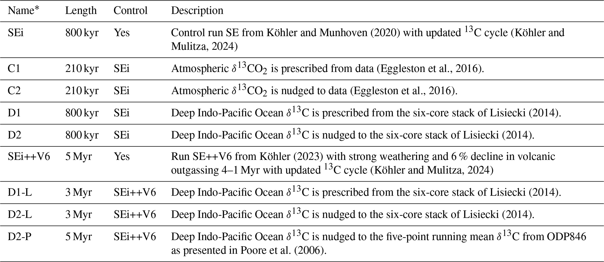
^* Naming convention: in non-control scenarios, the first letter indicates what kind of data are used (C: atmospheric δ¹³CO₂; D: deep Indo-Pacific δ¹³C), and the number indicates the form of data usage (1: prescribing; 2: nudging). Names with extended endings indicate 3–5 Myr long runs based on different data sets (-L: Lisiecki, 2014; -P: Poore et al., 2006).

Here, C(t) is the amount of carbon (in units gC) at time t in the atmosphere, when nudging to atmospheric δ¹³CO₂, or in the deep Indo-Pacific Ocean box, when nudging to deep Indo-Pacific δ¹³C, with $f_{{\mathrm{w}}_{\mathrm{Ca}}}\left(t\right)$ and f_v(t) being the annual fluxes (in units of gC yr⁻¹) in carbonate weathering and volcanic outgassing, respectively. The factor 0.5 in the denominator in Eq. (5) acknowledges that only half of the carbon in carbonate weathering has its source in weathered rock (e.g. Hartmann et al., 2009). In my 800 kyr long simulations, $f_{{\mathrm{w}}_{\mathrm{Ca}}}$ is constant at 12 Tmol yr⁻¹ (0.144 PgC yr⁻¹), while it varies as a function of CO₂ between 10–15 Tmol yr⁻¹ (0.12–0.18 PgC yr⁻¹) during the multi-million-year-long runs. The volcanic CO₂ outgassing flux (f_v(t)∼ 5–16 Tmol yr⁻¹ or 0.06–0.192 PgC yr⁻¹) is a 4 kyr time-delayed function of sea level change (Kutterolf et al., 2013).

I determined the strength η_DP=0.0001 when nudging to deep Indo-Pacific δ¹³C by comparing the resulting width of the distribution in ${\mathit{\delta }}^{\mathrm{13}}{\mathrm{C}}_{\mathrm{rock}}^{\mathrm{hypo}}\left(t\right)$ to the reconstructions (Fig. 3c). A comparable strength of the nudging is inversely related to the amount of carbon in the relevant box. Due to there being 30 times more carbon in the deep Indo-Pacific box than in the atmosphere, it was inferred that ${\mathit{\eta }}_{\mathrm{A}}={\mathit{\eta }}_{\mathrm{DP}}\cdot \mathrm{30}=\mathrm{0.003}$. For reasons of simplicity and due to a lack of data, the same nudging strength is used when calculating ${\mathit{\delta }}^{\mathrm{13}}{\mathrm{C}}_{\mathrm{v}}^{\mathrm{hypo}}\left(t\right)$.

In my setup, all CO₂ from volcanic outgassing is directly released into the atmosphere. It has been shown (Hasenclever et al., 2017) that submarine and subaerial injections of volcanic CO₂ lead to similar changes in the carbon cycle on multi-millennial timescales, making a distinction of volcanism in the two subgroups irrelevant here. Important for long-term CO₂ is the amount of carbon added to the atmosphere–ocean–biosphere system, not the location of the injection. This is also the reason why I investigate (a) how changes in δ¹³C_rock, which, as part of weathering (or of bicarbonate injection), enters the system in the surface ocean, might have an influence on atmospheric δ¹³CO₂ and (b) how both weathering and volcanism might change deep-ocean δ¹³C. Furthermore, these insights also suggest that, for cases of very strong nudging, as found in the prescribing scenarios, results can probably not be explained by isotopic signature changes in the external carbon fluxes.

As a final check for my hypothesis that the long-term changes in δ¹³C might be caused by the isotopic signature of the external sources to the carbon cycle, I compared δ¹³C from nudging scenarios with simulations in which either ${\mathit{\delta }}^{\mathrm{13}}{\mathrm{C}}_{\mathrm{rock}}^{\mathrm{hypo}}\left(t\right)$ or ${\mathit{\delta }}^{\mathrm{13}}{\mathrm{C}}_{\mathrm{v}}^{\mathrm{hypo}}\left(t\right)$, as derived from Eqs. (5)–(6), is externally prescribed (Fig. S4). Differences between both setups are generally less than 0.02 ‰ in various variables of the ¹³C cycle for the last 800 kyr, supporting my post-processing approach to reliably calculate the necessary isotopic signatures of these two fluxes in order to reduce the model–data offset in the ¹³C cycle.

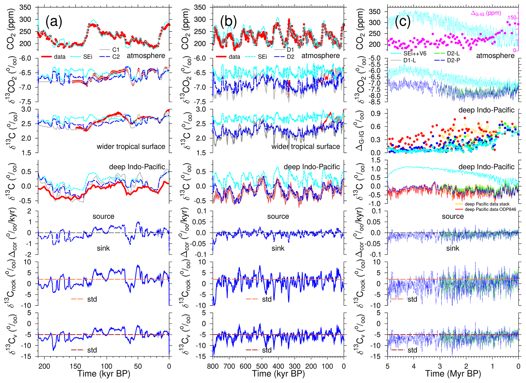
Figure 4 Closure of the ¹³C cycle on 405 kyr periodicity. From top to bottom: atmospheric CO₂, δ¹³CO₂, and δ¹³C in DIC of surface water of the wider tropics or in the deep Indo-Pacific; Δ_cor, ${\mathit{\delta }}^{\mathrm{13}}{\mathrm{C}}_{\mathrm{rock}}^{\mathrm{hypo}}$, and ${\mathit{\delta }}^{\mathrm{13}}{\mathrm{C}}_{\mathrm{v}}^{\mathrm{hypo}}$ for different scenarios, including reconstructions of CO₂ and δ¹³CO₂ (Bereiter et al., 2015; Eggleston et al., 2016; Krauss et al., 2025), and δ¹³C_DIC in the surface ocean of the wider tropics (anomalies to the LGM in the monospecific stack of G. ruber and Δ(δ¹³C_rub) from Köhler and Mulitza, 2024) or in the deep Pacific from the six-core stack (Lisiecki, 2014) or ODP846 (Poore et al., 2006). Δ_cor is calculated from (a) atmospheric δ¹³CO₂ or from (b, c) deep Indo-Pacific δ¹³C. In panel (c), Δ_G-IG is included for CO₂ (first row, right y axis) and (third row) Indo-Pacific δ¹³C (gold open circles for the 3 Myr long deep Pacific δ¹³C stack). No δ¹³C in DIC of the wider tropical surface ocean is plotted in panel (c). For Δ_G-IG, the difference between a glacial minimum and the subsequent interglacial maximum is calculated following the MIS boundary definition of Lisiecki and Raymo (2005), with points being positioned at mid-transitions. The results in Δ_cor, ${\mathit{\delta }}^{\mathrm{13}}{\mathrm{C}}_{\mathrm{rock}}^{\mathrm{hypo}}$, and ${\mathit{\delta }}^{\mathrm{13}}{\mathrm{C}}_{\mathrm{v}}^{\mathrm{hypo}}$ for the prescribed scenarios (C1, D1, D1-L) cover a wider range and are excluded here but are shown in Fig. S6.

2.2.3 Scenarios

My standard run (SEi) is based on the 800 kyr long scenario SE in Köhler and Munhoven (2020), with updates, mainly in the ¹³C cycle, as described in Köhler and Mulitza (2024). Prescribing and nudging to atmospheric δ¹³CO₂ (Eggleston et al., 2016) are performed in scenarios C1 and C2, respectively. Here, simulations are started at 210 kyr BP in the interglacial around MIS 7a-c, and the value of δ¹³CO₂ before 155 kyr is assumed to stay constant. The whole 800 kyr long runs are alternatively prescribed with (D1) and nudged to (D2) the deep Pacific δ¹³C stack. For an even longer perspective, I rely on the 5 Myr long runs published in Köhler (2023). Here, I choose a scenario based on run SE++V6, in which weathering is strongly coupled to atmospheric CO₂ and volcanic outgassing decreases by 6 % between 4 and 1 Myr BP, leading to a gradual decline in atmospheric CO₂. Tests have shown that the findings I describe further below are also robust for other scenarios included in Köhler (2023), with different weathering strength and volcanic history leading to alternative atmospheric CO₂ time series. Even when forced with the new 4.5 Myr long compilation of changes in surface temperature (Clark et al., 2024), which contains some power in periodicities slower than 100 kyr, my conclusions stay the same. I distinguish between a control run (SEi++V6), 3 Myr long runs in which deep Indo-Pacific δ¹³C is either prescribed with (D1-L) or nudged to (D2-L) the δ¹³C stack from Lisiecki (2014), and a 5 Myr long run (D2-P) nudged to δ¹³C in ODP846 as presented in Poore et al. (2006). An overview of all scenarios is compiled in Table 1.

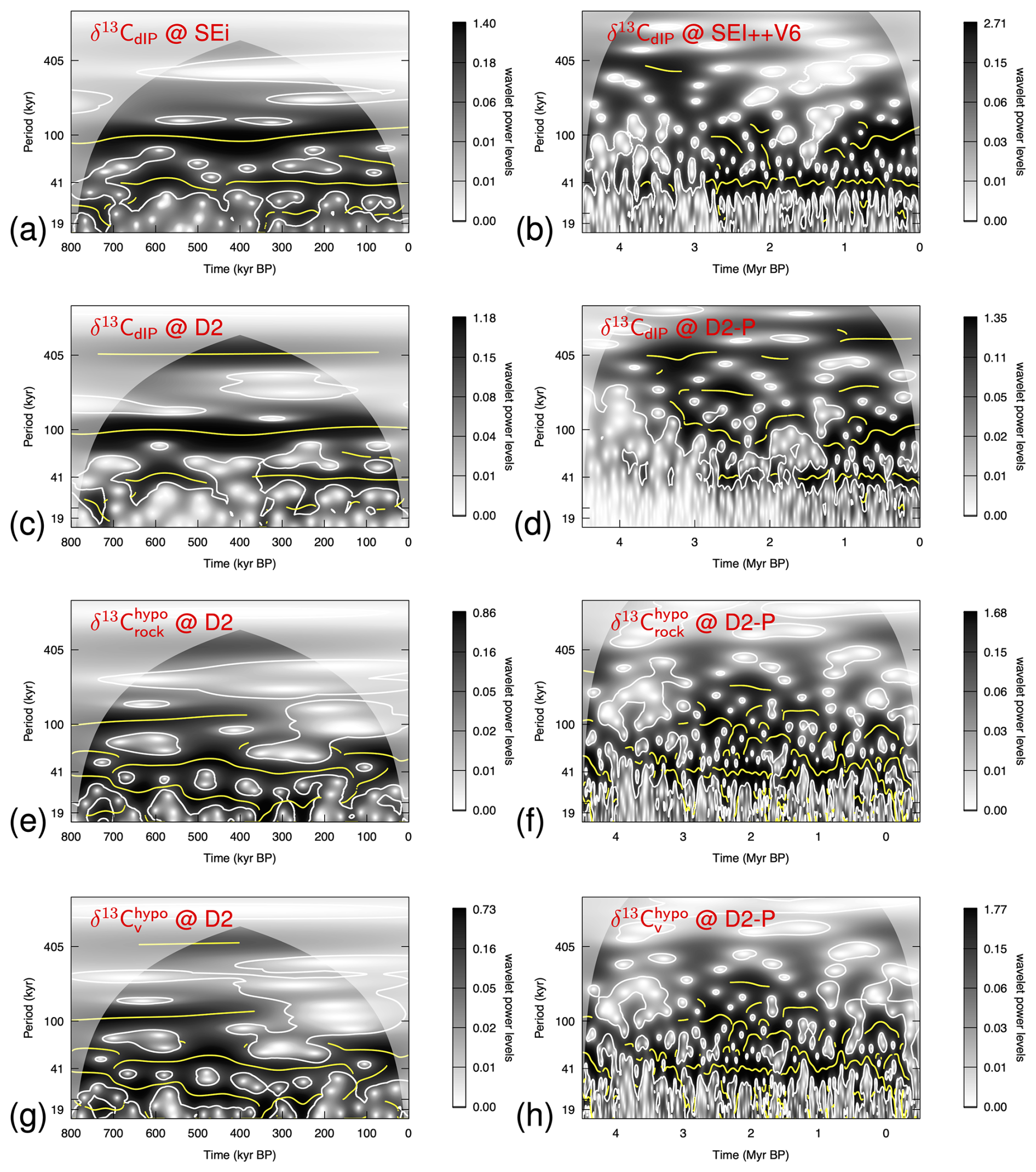
Figure 5 Wavelets of either the deep Indo-Pacific δ¹³C (a–d) or my solution for (e, f) ${\mathit{\delta }}^{\mathrm{13}}{\mathrm{C}}_{\mathrm{rock}}^{\mathrm{hypo}}$ and (g, h) ${\mathit{\delta }}^{\mathrm{13}}{\mathrm{C}}_{\mathrm{v}}^{\mathrm{hypo}}$ for different scenarios (left: SEi or D2; right: SEi++V6 or D2-P). Results are restricted to the last 4.5 Myr to avoid long spinup effects, and only data in panel (b) were detrended before spectral analysis.

2.3 Analysis tools

I use R (R Core Team, 2023) for calculating wavelets with WaveletComp (Roesch and Schmidbauer, 2018) and the package seewave, version 2.2.3, for further frequency analysis including coherence. In all wavelet figures, the white lines mark the 0.1 significant level and the yellow lines mark the ridges of the power distribution. Detrending of data was performed with MATLAB (The MathWorks Inc., 2023).

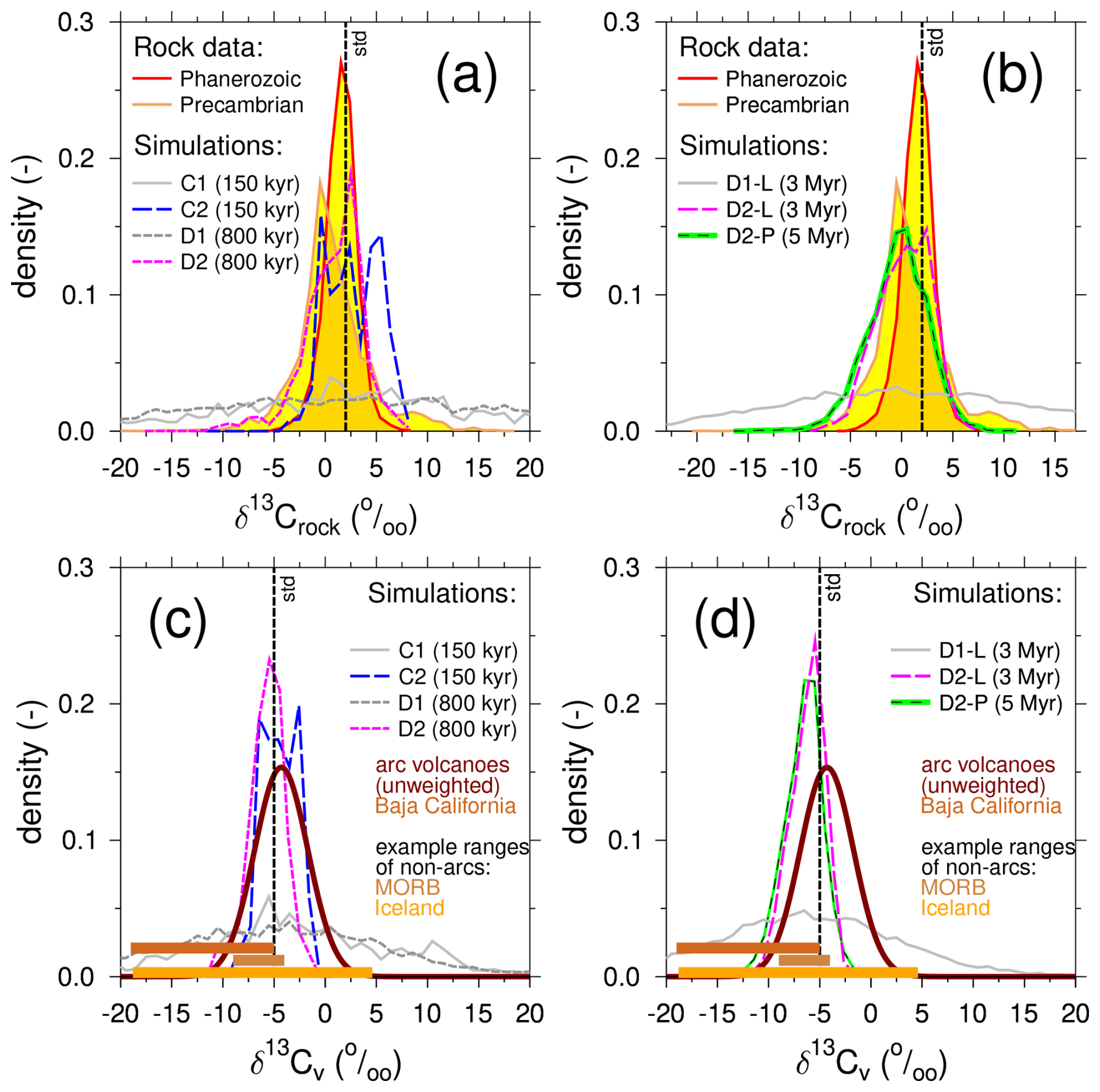
Figure 6 Distribution of the carbon isotopic signature of (a, b) carbonate rock (δ¹³C_rock) and of (c, d) volcanic CO₂ (δ¹³C_v) from Earth's history in data and simulations. More details on the rock data are found in Fig. 3. Simulations up to 800 kyr long (a, c) versus multi-million-year-long simulations (b, d). The δ¹³C_v data in panels (c) and (d) are from modern observations. The distribution of δ¹³C_v data, not weighted by CO₂ fluxes, from the review of arc volcanoes (Mason et al., 2017) is shown here under the assumption of a normal distribution with mean ±1σ of $-\mathrm{4.3}\pm \mathrm{2.6}$ ‰. Additionally, the range of data from newer studies on arc volcanism in Baja California (Batista Cruz et al., 2019; Barry et al., 2020) and the exemplary ranges from non-arc volcanism of mid-ocean ridge basalt (MORB) (Sano and Williams, 1996) and Iceland (Barry et al., 2014) are given. Vertical broken lines mark the standard (std) parameter values used in the model.

3 Results

Atmospheric CO₂ as simulated in my scenarios is shown as a control (Fig. 4, first row) against data (Bereiter et al., 2015). This is chosen here as an indicator of the dynamics of the carbon cycle, in depth discussions of which are covered in previous papers (Köhler and Munhoven, 2020; Köhler, 2023).

The control simulations (without prescription or nudging to δ¹³C) contain typical multi-millennial variations of the order of 0.5 ‰ in atmospheric δ¹³CO₂ (Fig. 4, second row) and 0.3 ‰ in δ¹³C_DIC of the wider tropical surface ocean (Fig. 4, third row) and G-IG variations of 0.5 ‰ in δ¹³C_DIC of the deep Indo-Pacific (Figs. 4, fourth row) during the Late Pleistocene. As shown before (Köhler and Mulitza, 2024), atmospheric δ¹³CO₂ and δ¹³C_DIC of the wider tropical surface ocean are highly correlated on orbital timescales of 41 kyr periodicities. In scenarios C1 (prescribed δ¹³CO₂) and C2 (nudged to δ¹³CO₂), there is also a loose correlation between atmospheric δ¹³CO₂ and deep Indo-Pacific δ¹³C on these timescales (Fig. S5), with a coherence that rose from below 0.2 in scenario SEi to 0.6 (C1) or 0.4 (C2). A tighter correlation between δ¹³C in the deep ocean and the atmosphere is not expected, since the marine carbon pumps introduce vertical gradients in δ¹³C (e.g. Schmittner et al., 2013), with opposite effects on atmospheric δ¹³CO₂ (or surface-ocean δ¹³C) and deep-ocean δ¹³C on G-IG timescales (Köhler et al., 2010). Therefore, there has to be a certain anti-correlation between atmospheric δ¹³CO₂/surface-ocean δ¹³C on the one hand and deep Pacific δ¹³C on the other hand. In other words, prescribing or nudging to atmospheric δ¹³CO₂ or deep Pacific δ¹³C always increases the agreement of the simulations to the reconstructions in the other variable, but a perfect fit in the other endmember of the ¹³C cycle is not expected. In scenarios C2 and D2, the long-term evolution from PGM to LGM in both atmospheric δ¹³CO₂ and wider surface-ocean δ¹³C is covered in the simulations, but the local maxima in the data around 80 kyr BP are not contained, suggesting that internal processes in the atmosphere–ocean–biosphere subsystem rather than these solid Earth fluxes are responsible for these anomalies, which occur on shorter timescales. Millennial-scale changes in atmospheric δ¹³CO₂ between 70 and 60 kyr BP have already been successfully explained by such internal processes, namely rapid changes in terrestrial carbon pools and/or Southern Ocean air–sea gas exchange (Menking et al., 2022), which were probably also active around 80 kyr BP.

The introduction of the long-term periodicities into my simulated ¹³C cycle can be seen in the spectral analysis. Wavelets show, apart from the time window 4–3 Myr BP, no power in periodicities beyond 100 kyr in the deep Indo-Pacific δ¹³C in the control simulations SEi and SEi++V6 (Fig. 5a, b), but simulations contain power comparable to the data around 400 kyr and also in 200 kyr periodicities when nudged to the reconstructions (Figs. 1c, d and 5c, d). I therefore conclude that, on these slow timescales, my nudged simulations are in reasonable agreement with the data.

The time series of ${\mathit{\delta }}^{\mathrm{13}}{\mathrm{C}}_{\mathrm{rock}}^{\mathrm{hypo}}$ or ${\mathit{\delta }}^{\mathrm{13}}{\mathrm{C}}_{\mathrm{v}}^{\mathrm{hypo}}$ necessary to close the ¹³C cycle in the long eccentricity timescale are found in the two lowermost rows of Fig. 4 for the nudged scenarios (C2, D2, D2-L, D2-P), while those of the prescribed scenarios (C1, D1, D1-L) are due to the larger data scatter plotted with different y axes in Fig. S6, which otherwise repeats Fig. 4. The resulting density distributions of both ${\mathit{\delta }}^{\mathrm{13}}{\mathrm{C}}_{\mathrm{rock}}^{\mathrm{hypo}}$ and ${\mathit{\delta }}^{\mathrm{13}}{\mathrm{C}}_{\mathrm{v}}^{\mathrm{hypo}}$, together with the data constraints, are compiled in Fig. 6. When prescribing one δ¹³C record from data (scenarios C1, D1, D1-L), it is clearly seen that the necessary distributions of the parameter values are with 1σ>14 ‰ (${\mathit{\delta }}^{\mathrm{13}}{\mathrm{C}}_{\mathrm{rock}}^{\mathrm{hypo}}$) and 1σ>9 ‰ (${\mathit{\delta }}^{\mathrm{13}}{\mathrm{C}}_{\mathrm{v}}^{\mathrm{hypo}}$) much wider than what reconstructions are suggesting (1σ<4 ‰ for δ¹³C_rock and 1σ<3 ‰ for δ¹³C_v from present-day arc volcanoes). This finding indicates that a prescription of δ¹³C, during which the model would follow the reconstruction not only on orbital timescales but also during shorter multi-millennia anomalies, cannot be explained by the isotopic signature of either carbonate rock or volcanic outgassing. In other words, the scenarios C1, D1, and D1-L are unrealistic with respect to an explanation of the 405 kyr periodicity in the ¹³C cycle and can be discarded here.

In the nudged simulations (scenarios C2, D2, D2-L, D2-P), the resulting ${\mathit{\delta }}^{\mathrm{13}}{\mathrm{C}}_{\mathrm{rock}}^{\mathrm{hypo}}$ and ${\mathit{\delta }}^{\mathrm{13}}{\mathrm{C}}_{\mathrm{v}}^{\mathrm{hypo}}$ vary on orbital (and sometimes faster) timescales over the whole parameter range provided by the reconstructions (Fig. 4). While these dynamics challenge our understanding of which processes might have been responsible for them (see Discussion), the resulting statistics (density distributions) are not unreasonable (Fig. 6). In detail, the nudged 800 kyr long simulations overlap well with the Phanerozoic reconstructions of δ¹³C in carbonate rock (D2: 0.8 ± 3.0 ‰), while, in longer simulations, I find even tighter distributions but with lower mean values (D2-L: 0.2 ± 2.6 ‰; D2-P: $-\mathrm{0.4}\pm$ 3.0 ‰) more in agreement with the Precambrian δ¹³C rock data (Fig. 6a, b). Similarly, the mean in ${\mathit{\delta }}^{\mathrm{13}}{\mathrm{C}}_{\mathrm{v}}^{\mathrm{hypo}}$ is lower in nudged multi-million-year simulations than in those covering only 800 kyr (D2: $-\mathrm{5.1}\pm$ 2.0 ‰; D2-L: $-\mathrm{6.2}\pm$ 1.7 ‰; D2-P: $-\mathrm{6.6}\pm$ 2.0 ‰), and the distributions are, at 1σ≤2 ‰, sufficiently narrow and overlap with data of δ¹³C in volcanic CO₂ (Fig. 6c, d). Remember that the nudging strength η_DP was determined from the width of the distribution of ${\mathit{\delta }}^{\mathrm{13}}{\mathrm{C}}_{\mathrm{rock}}^{\mathrm{hypo}}$ in scenario D2 to be comparable to the data but that its mean value was never used as a tuning target: it freely evolved from the simulations and the post-processing analysis. The shift towards lower mean values in ${\mathit{\delta }}^{\mathrm{13}}{\mathrm{C}}_{\mathrm{rock}}^{\mathrm{hypo}}$ or ${\mathit{\delta }}^{\mathrm{13}}{\mathrm{C}}_{\mathrm{v}}^{\mathrm{hypo}}$ for longer simulations is dominantly caused by δ¹³C in ODP846 (used for nudging in scenario D2-P) being on average lower than δ¹³C in the deep Pacific stack (used for nudging in scenarios D2 and D2-L).

When nudging to δ¹³CO₂ (scenario C2), I obtain a rather skewed distribution of ${\mathit{\delta }}^{\mathrm{13}}{\mathrm{C}}_{\mathrm{rock}}^{\mathrm{hypo}}$ (2.7±2.6 ‰) which is wider than the reconstruction from carbonate rock (Fig. 6a). The width of the solution does not improve if I revise the nudging strength η_A within reasonable bounds. Thus, it seems that the shortness of the δ¹³CO₂ time series, which covers not even half of one long eccentricity cycle, is responsible for this unsatisfactory result. The distribution for ${\mathit{\delta }}^{\mathrm{13}}{\mathrm{C}}_{\mathrm{v}}^{\mathrm{hypo}}$ ($-\mathrm{4.5}\pm \mathrm{1.7}$ ‰) in scenario C2 has a slightly larger mean value, but its width is similar to what I obtain in scenario D2 from longer runs and nudging to deep Pacific δ¹³C ($-\mathrm{5.7}\pm \mathrm{1.9}$ ‰). However, the shape of the distribution for C2 is, without a clear maximum, very different from a bell-shaped Gaussian curve of a normal distribution (Fig. 6c). As this analysis initially starts from understanding δ¹³CO₂, the available data do not yet cover a sufficiently long period for a complete understanding of the 405 kyr cycle in them, although the recently published new data around 340 kyr BP (Krauss et al., 2025) fully support my findings so far, where δ¹³CO₂ ranges between −6.8 ‰ and −7.3 ‰, much lower than in scenario SEi but in agreement with my scenario D2 (Fig. 4b).

As a side effect, my nudging approach also increases the G-IG amplitudes in the simulated ¹³C cycle before the MPT. In the data and in the prescribed scenario D1-L, the G-IG amplitudes in deep Indo-Pacific δ¹³C were only reduced to 75 % of their post-MPT size prior to the MPT, while, in the control run SEi++V6, they were reduced to 24 % (Figs. 1a, 4c). My nudging approach increases these pre-MPT G-IG amplitudes to 41 % (D2-L) and 32 % (D2-P) of their amplitudes during the last 1 Myr, thus partially explaining this feature of the 41 kyr world (Fig. 4c).

Altogether, I conclude that the carbon isotopic signature of either carbonate rocks or volcanic CO₂ outgassing might be the process which closes the ¹³C cycle on periodicities slower than 100 kyr in the Plio-Pleistocene. Furthermore, the PGM-to-LGM offset in atmospheric δ¹³CO₂ and the long eccentricity in benthic δ¹³C are potentially caused by the same processes and are therefore related to each other.

4 Discussion

A frequency analysis of the derived solutions for ${\mathit{\delta }}^{\mathrm{13}}{\mathrm{C}}_{\mathrm{rock}}^{\mathrm{hypo}}$ and ${\mathit{\delta }}^{\mathrm{13}}{\mathrm{C}}_{\mathrm{v}}^{\mathrm{hypo}}$ (Fig. 5e–h) finds that only little power is contained in periodicities beyond 100 kyr. Results for both variables are dominated by power in the obliquity band and some contributions to the 100 kyr band. Between 2–3 Myr BP, some enhanced power in the 200 kyr periods is contained in both solutions obtained from scenario D2-P. Modifications in either ${\mathit{\delta }}^{\mathrm{13}}{\mathrm{C}}_{\mathrm{rock}}^{\mathrm{hypo}}$ or ${\mathit{\delta }}^{\mathrm{13}}{\mathrm{C}}_{\mathrm{v}}^{\mathrm{hypo}}$, both with little power around 405 kyr, lead nevertheless to a persisting occurrence of the long eccentricity in the resulting ¹³C cycle. A transition of power to other frequencies was suggested to be caused by the long residence time of carbon in the ocean during earlier quasi-ice-free periods of the Cenozoic (Pälike et al., 2006; Zeebe et al., 2017). However, the power transition was probably happening for other reasons, since the main carbon cycle and CO₂ contain no power in 405 kyr periodicity (Fig. 2g–i), which was not the case in these other studies. Looking closer at the spectra of the resulting simulated deep Indo-Pacific δ¹³C and the inversely obtained ${\mathit{\delta }}^{\mathrm{13}}{\mathrm{C}}_{\mathrm{rock}}^{\mathrm{hypo}}$ (or ${\mathit{\delta }}^{\mathrm{13}}{\mathrm{C}}_{\mathrm{v}}^{\mathrm{hypo}}$) for the same scenario, I find that the relative power in obliquity (41 kyr) and long eccentricity (405 kyr) is actually similar in both variables (Fig. S7). This similarity, not necessarily obtained from the related wavelets (Fig. 5d, f), supports the connection between both variables and highlights that obliquity is indeed the most important in both time series, while 405 kyr is only weakly contained. Thus, it is not surprising that little 405 kyr power in deep Indo-Pacific δ¹³C is derived from ${\mathit{\delta }}^{\mathrm{13}}{\mathrm{C}}_{\mathrm{rock}}^{\mathrm{hypo}}$ (or ${\mathit{\delta }}^{\mathrm{13}}{\mathrm{C}}_{\mathrm{v}}^{\mathrm{hypo}}$), with similarly little relative power in the same frequency band.

To better understand how variations in δ¹³C_rock or δ¹³C_v with orbital frequencies impact on deep-ocean δ¹³C, I performed some tests. Using time series of the orbital parameters eccentricity, climate precession, and obliquity (Laskar et al., 2004), artificial changes in δ¹³C_rock or δ¹³C_v were generated with patterns (mean, σ) similar to the reconstructions and then applied to some forward simulations modifying the control run SEi. The results (Fig. S8) show that δ¹³C_v has a larger effect than δ¹³C_rock on deep Indo-Pacific δ¹³C, probably because the related carbon influx (CO₂ outgassing) is about twice as large as that of carbonate rock during weathering. Furthermore, the resulting deep-ocean δ¹³C anomalies with respect to SEi are lagging the forcing by about a quarter of the forcing periodicities. This is happening for all orbital forcings and frequencies indicating the time delay by which the deep-ocean δ¹³C reacts to changes in the geological isotopic signatures. In other words, the change in δ¹³C_rock or δ¹³C_v obtained in the nudging approach, which is suggested to be responsible for the slow variations (405 kyr periodicity) in deep-ocean δ¹³C, is delayed accordingly. Although this lag might not be important for the spectra of δ¹³C_rock or δ¹³C_v it might need consideration if the hypothesis here is tested in future studies in forward simulations (see below). Furthermore, this lag suggests that the proposed solutions in δ¹³C_rock or δ¹³C_v might lead to some extent to overshooting/undershooting in the target variable, which would influence the amplitudes but not the frequencies. However, since the obtained distributions in both variables are already in agreement with the reconstructions, smaller ranges would only increase their match to the data.

The chosen setup restricted my analysis to the inversely obtained changes in the isotopic signatures of the geological sources. Therefore, the changes in ${\mathit{\delta }}^{\mathrm{13}}{\mathrm{C}}_{\mathrm{rock}}^{\mathrm{hypo}}$ and ${\mathit{\delta }}^{\mathrm{13}}{\mathrm{C}}_{\mathrm{v}}^{\mathrm{hypo}}$ are not correlated to the underlying carbon fluxes (r²<0.01), although volcanism was partly a function of the obliquity-dominated changes in sea level/land ice volume and the strength of the carbonate weathering in multi-million-year-long runs was related to CO₂, which is also dominated by obliquity (Fig. 2e). Such relationships between fluxes and isotopic signatures, if found, might give further support to this hypothesis, since such connections might be expected from a process-based perspective. However, previous model results have shown that changing the strength of fluxes without compensating effects very likely changes not only the ¹³C cycle but also the underlying main carbon cycle (Russon et al., 2010). Thus, such results are not easily obtained but might be searched for in future studies.

Obliquity has an influence on incoming solar radiation in the high latitudes and is therefore thought to be the main control for land ice dynamics in the Northern Hemisphere (e.g. Huybers, 2007; Willeit et al., 2019; Köhler and van de Wal, 2020). Thus, obliquity, together with some influence of precession (Huybers, 2011; Barker et al., 2025) and internal feedbacks (e.g. Willeit et al., 2019; Berends et al., 2021; Clark et al., 2024), determines the G-IG cyclicity of the Plio-Pleistocene. Therefore, the dominance of obliquity in my solutions for either ${\mathit{\delta }}^{\mathrm{13}}{\mathrm{C}}_{\mathrm{rock}}^{\mathrm{hypo}}$ or ${\mathit{\delta }}^{\mathrm{13}}{\mathrm{C}}_{\mathrm{v}}^{\mathrm{hypo}}$ suggests that land ice might also play an important role in my closure of the ¹³C cycle for slow timescales of the Plio-Pleistocene.

Previously, the Pleistocene 400–500 kyr periodicity in marine δ¹³C was suggested to have been caused by continental weathering and monsoon activity (Wang et al., 2010, 2014), and climate simulations also highlight the role of the 405 kyr periodicity in tropical precipitation (Yun et al., 2023). The Asian monsoon during the last 650 kyr as deduced from detrended δ¹⁸O in speleothems has significant power in obliquity but in antiphase to summer insolation at 65° N, which suggests that the ultimate cause for the 41 kyr related changes are situated in the Northern Hemisphere ice sheets (Cheng et al., 2016). Furthermore, present-day reconstructions of the continental weathering rates indicate that highly active regions dominate the global signal, with 10 % of the area contributing about 50 % of the global weathering fluxes (Hartmann et al., 2009). This study and others (Hartmann and Moosdorf, 2011; Moosdorf et al., 2011; Börker et al., 2020) also identified runoff, which is highly related to precipitation, as one of the dominant controls of local weathering fluxes. Obliquity-controlled monsoon systems therefore have a leverage on weathering, potentially activating contributions from different regions on Earth, with variable δ¹³C_rock, accordingly. I therefore suggest that obliquity-driven changes might also easily control the weathering strength of different areas, finally ending in changes in ${\mathit{\delta }}^{\mathrm{13}}{\mathrm{C}}_{\mathrm{rock}}^{\mathrm{hypo}}$ without the need for large variations in the global weathering flux itself. This influence of obliquity might operate via monsoon, but a variable contribution of available weatherable rock around dynamic ice sheets in North America and Eurasia or from continental shelves during sea level low stands also seems possible (e.g. Börker et al., 2020).

Dominant power in the obliquity band is also contained in the reconstructed activity of the circum-Pacific chain of arc volcanism, sometimes referred to as the “Ring of Fire”, during the last 1 Myr (Kutterolf et al., 2013). In a revised analysis, this power in 41 kyr is reduced and is only second behind 100 kyr (Kutterolf et al., 2019). This spectral analysis supports hypotheses that changes in land ice load or sea level might influence subaerial or submarine volcanism, respectively (Huybers and Langmuir, 2009, 2017; Hasenclever et al., 2017). Note that, in the model, the component of volcanic CO₂ outgassing that is influenced by either land ice or sea level changes is lagging them by 4 kyr (Kutterolf et al., 2013). In light of known temporal changes in the isotopic signature of individual volcanoes (e.g. Chiodini et al., 2011) and of the large heterogeneity of the mantle material (e.g. Moussallam et al., 2024), the obliquity-related changes in ${\mathit{\delta }}^{\mathrm{13}}{\mathrm{C}}_{\mathrm{v}}^{\mathrm{hypo}}$, as inversely deduced here from the analysis, are therefore also conceivable.

Possible ways of testing the proposed hypothesis of the obliquity-dominated influence on the isotopic signature of the geological sources might be the following. The most direct support might be derived from a forward modelling approach in which the isotopic signature of the geological sources and the strength of the related fluxes are correlated to each other. This would, however, need a data-mining effort, in which fluxes and isotopic signature are spatially connected for the present day. This approach might not generate long time series as done here, but it tries to establish if fast changes in global mean ${\mathit{\delta }}^{\mathrm{13}}{\mathrm{C}}_{\mathrm{rock}}^{\mathrm{hypo}}$ or ${\mathit{\delta }}^{\mathrm{13}}{\mathrm{C}}_{\mathrm{v}}^{\mathrm{hypo}}$, as suggested here, are feasible from a more process-based understanding. However, unknown mantle heterogeneity and unknown temporal evolution of both local fluxes and local isotopic signatures might make this a rather challenging task. Frequency analysis of various weathering proxies (e.g. Vance et al., 2009; von Blanckenburg et al., 2015) obtained from sediment cores in different ocean basins might give indications if obliquity played a dominant role on the regional scale, although this would only give indirect evidence on flux strength and not on δ¹³C_rock. Monitoring programmes on present-day volcanoes might give a broader foundation if temporal changes in δ¹³C_v, as observed for the Etna, are an exception or the rule (Chiodini et al., 2011). Finally, the connection of the PGM and LGM offset in atmospheric δ¹³CO₂, and how this is related to the 405 kyr periodicity, might be verified with new ice core data of atmospheric δ¹³CO₂ further back in time.

5 Conclusions

My analysis, based on an inverse approach which nudged simulated δ¹³C time series to reconstructions, suggests that variations in the isotopic signatures of the geological sources (δ¹³C of weathered carbonate rock or δ¹³C of volcanic outgassed CO₂) might, without any further changes in the carbon cycle, be sufficient to explain the signals in δ¹³C related to the long eccentricity cycle during most of the Plio-Pleistocene. Furthermore, my suggested solution connects this periodicity around 405 kyr in deep-ocean δ¹³C with the PGM-to-LGM offset in atmospheric δ¹³CO₂, implying that both are caused by the same underlying processes. My analysis highlights the influence of obliquity on these changes in the ¹³C cycle, which I interpret as Northern Hemisphere ice sheets being the ultimate cause for the necessary variations in δ¹³C_rock or δ¹³C_v. Studies show that both weathering and volcanic activity might, directly or indirectly, be influenced by land ice dynamics, giving independent support for my hypothesis. Taking the link to obliquity for granted, it is furthermore unlikely that the same mechanisms might have been responsible for the 405 kyr periodicity in marine δ¹³C found in earlier climates of the Cenozoic, since there has not been any substantial Northern Hemisphere ice sheet (Pälike et al., 2006; Zeebe et al., 2017; De Vleeschouwer et al., 2020; Westerhold et al., 2020). During these times, not only δ¹³C, but also δ¹⁸O and potentially atmospheric CO₂, contained cyclicity related to the long eccentricity, which is missing here for the Plio-Pleistocene; this requires other solutions to the problem. However, both my possible answers, either via carbonate weathering or via volcanism, seem similarly likely. So far, I have not yet found a criterion which makes one more likely than the other, and a mixture of both is probably the most realistic solution to the closure of the ¹³C cycle on these slow timescales suggested here. However, as outlined in the Discussion, further investigations and proposed tests might favour one above the other. The dominance of obliquity in my solutions readily explains an improvement in simulated G-IG amplitudes in δ¹³C in the 41 kyr world of the Plio-Pleistocene, but their reconstructed sizes are not fully obtained. Thus, while the influence of the isotopic signature of the geological sources might be important for the decoupling of climate from the carbon cycle, there is room for other (not yet detected) processes for a complete understanding of the Plio-Pleistocene ¹³C cycle.