Equilibrium line altitudes of alpine glaciers in Alaska suggest Last Glacial Maximum summer temperature was 2–5 °C lower than during the pre-industrial

The lack of continental ice sheets in Alaska during the Last Glacial Maximum (LGM; 26–19 ka) has long been attributed to extensive aridity in the western Arctic. More recently, climate model outputs, a few isolated paleoclimate studies, and global paleoclimate synthesis products show mild summer temperature depressions in Alaska compared to much of the high northern latitudes. This suggests the importance of limited summer temperature depressions in controlling the relatively limited glacier growth during the LGM. To explore this further, we present a new statewide map of LGM alpine glacier equilibrium line altitudes (ELAs), LGM ΔELAs (LGM ELA anomalies relative to the Little Ice Age, LIA), and ΔELA-based estimates of temperature depressions across Alaska to assess paleoclimate conditions. We reconstructed paleoglacier surfaces in ArcGIS to calculate ELAs using an accumulation area ratio (AAR) of 0.58 and an area–altitude balance ratio (AABR) of 1.56. We calculated LGM ELAs (n= 480) in glaciated massifs in the state, excluding areas in southern Alaska that were covered by the Cordilleran Ice Sheet. The data show a trend of increasing ELAs from the southwest to the northeast during both the LGM and the LIA, indicating a consistent southern Bering Sea and northernmost Pacific Ocean precipitation source. Our LGM–LIA ΔELAs from the Alaska Range, supported with limited LGM–LIA ΔELAs from the Brooks Range and the Kigluaik Mountains, average to −355 ± 176 m. This value is much greater than the global LGM average of ca. −1000 m. Using a range of atmospheric lapse rates, LGM–LIA ΔELAs in Alaska translate to summer cooling of < 2–5 ^∘C. Our results are consistent with a growing number of local climate proxy reconstructions and global data assimilation syntheses that indicate mild summer temperature across Beringia during the LGM. Limited LGM summer temperature depressions could be explained by the influence of Northern Hemisphere ice sheets on atmospheric circulation.

1 Introduction

Unlike much of northern North America and western Eurasia, Alaska remained largely free of continental ice sheets throughout the late Pleistocene. Most alpine glaciers and ice sheets across North America reached their late Pleistocene maxima during Marine Isotope Stage 2 (MIS 2; generally known as the Last Glacial Maximum, LGM; 26–19 ka). However, it has been recognized for decades that ice masses in Alaska reached their greatest extents earlier in the last glacial cycle, with comparatively limited glaciation during MIS 2. Early studies hypothesized these maxima occurred during MIS 4 or 6, before absolute age chronologies dated these to MIS 4 (Briner et al., 2001, 2005; Coulter et al., 1965; Kaufman et al., 2011; Péwé, 1975, 1953; Tulenko et al., 2018). The relative lack of glaciation in Alaska suggests drier conditions and/or milder temperatures during the LGM compared to other parts of the high-latitude Northern Hemisphere (i.e., Arctic Canada, western Eurasia, and Greenland). Indeed, researchers have long attributed the lack of ice sheets to widespread aridity across Alaska (e.g., Capps, 1932; Hamilton, 1994). Other studies also hypothesized that mild temperatures (in addition to arid conditions) led to limited ice sheet development across Alaska (Briner and Kaufman, 2008; Péwé, 1975). Alaskan lacustrine paleoclimate proxy studies (e.g., Abbott et al., 2010; Bartlein et al., 2011; Finkenbinder et al., 2014, 2015; Daniels et al., 2021; King et al., 2022; Kurek et al., 2009; Viau et al., 2008) and blending of proxy-based sea-surface temperatures with a global climate model (e.g., Osman et al., 2021; Tierney et al., 2020a) suggest that Alaska was comparatively warm and dry during the LGM. Paleoclimate models support mild temperatures in Alaska during the LGM but disagree on whether Alaska was slightly warmer or slightly colder than during the pre-industrial period (Kageyama et al., 2021; Löfverström and Liakka, 2016; Löfverström et al., 2014; Otto-Bliesner et al., 2006).

Disagreement between proxy, data assimilation, and model results highlight their respective strengths and weaknesses. Lacustrine proxy data generally offer more ground truth data at a fine resolution, but such studies are time- and labor-intensive and are confined to relatively small geographic areas. Data assimilation products can provide broad spatial coverage but thus far have used relatively geographically limited terrestrial datasets or more ubiquitous marine records and projected reconstructed temperatures onto land (Annan et al., 2022; Osman et al., 2021; Tierney et al., 2020a). Climate models similarly achieve good spatial coverage but lack widespread tie points, useful for evaluating the veracity of certain models. Despite progress in both data assimilation and climate model development, the limited availability of terrestrial records highlights a need to provide ground-truth paleoclimate data across large geographic areas – especially in Alaska – where studies suggest surprisingly mild conditions, compared to adjacent areas of North America.

There are limited paleoclimate proxy datasets in Alaska that extend back to the LGM. However, we can assess paleoclimate conditions during the LGM across much of the state by reconstructing equilibrium line altitudes (ELAs) of former glaciers that have been widely mapped and in places, dated. Additionally, glaciers in Alaska were at climatic equilibrium during the Little Ice Age (LIA; ∼ 19th century) before the industrial period and deposited moraines marking their extents, thus serving as a useful pre-industrial climate reference (Barclay et al., 2009; Molnia, 2008; Solomina et al., 2015). Comparing LGM and LIA ELAs allows us to assess relative differences in climate between the two time periods (e.g., Federici et al., 2008).

Here, we present ELA reconstructions for 480 alpine glaciers in Alaska to test the hypothesis that minor temperature depressions – in addition to aridity – explain limited glaciation in Alaska during the LGM. We used the Alaska PaleoGlacier Atlas v2 (Kaufman et al., 2011) and high-resolution digital elevation models (DEMs) to map LGM extents, the GlaRe GIS tool to synthesize paleoglacier surfaces, and a GIS ELA calculation tool to evaluate LGM climate (Pellitero et al., 2015, 2016). We used similar methods to reconstruct LIA ELAs (and consider this the pre-industrial period) and then calculated ΔELAs (LGM_ELA-LIA_ELA) and temperature depressions from the Alaska Range, with more limited data from across the state. We find that distance from a northern Pacific moisture source exercised a strong control on ELAs across Alaska during both the LGM and the LIA and our ELA-based paleotemperature reconstructions agree with recent model and paleoclimate data synthesis products showing relatively low LGM temperature depressions in Alaska.

2 Background

Alpine glaciers are robust indicators of climate as their extent is primarily controlled by summer temperatures and annual precipitation (Benn and Lehmkuhl, 2000; Ohmura et al., 1992; Ohmura and Boettcher, 2018; Kurowski, 1891; Roe et al., 2017; Rupper and Roe, 2008; Sutherland, 1984; Walcott, 2022). Numerous studies have compared ELAs of reconstructed LGM glaciers worldwide to ELAs of extant glaciers (e.g., Kłapyta et al., 2021), ELAs of reconstructed LIA glaciers (Federici et al., 2008), or hypothetical ELAs in the atmosphere (Ono et al., 2005) and used atmospheric lapse rates to estimate LGM temperature depressions. Additionally, several numerical models of alpine paleoglaciers have been developed that quantify paleotemperature and paleoprecipitation conditions (e.g., Leonard et al., 2017; Plummer and Phillips, 2003). However, modeling individual alpine glaciers is often time-consuming and computer-intensive and therefore better suited for smaller geographic areas. ELA reconstructions, on the other hand, are relatively labor efficient and more easily applied to a large region (e.g., Brooks et al., 2022; Rea et al., 2020). Of course, both methods rely on immense amounts of chronology and field mapping required to designate accurate LGM alpine glacier limits.

Glaciation across Alaska during the LGM was largely restricted to dozens of isolated massifs and mountain ranges across the state, rather than large continental ice sheets seen elsewhere in the Northern Hemisphere (Fig. 1). Much of the Brooks Range was covered by extensive interconnected valley glacier systems; poorly constrained “ice sheds” in the high icefield areas preclude using traditional methods in ELA reconstruction (Hamilton and Porter, 1975; Kaufman et al., 2011). However, numerous valleys outside of the central ice mass in the Brooks Range hosted well-defined cirque and valley glaciers during the LGM. While much of the south-central and southeastern Alaska Range was covered by the Cordilleran Ice Sheet – hampering ELA reconstructions there – there were well-defined and often-extensive glaciers present in the outward-facing (north and west) valleys. The Ahklun Mountains were smothered by an ice cap, though several portions of the outlying mountains hosted isolated valley glaciers. Outside of these areas, alpine glaciers were present during the LGM within smaller massifs across much of the state from the Yukon–Tanana Uplands to the Seward Peninsula (Coulter et al., 1965; Kaufman et al., 2011; Péwé, 1975).

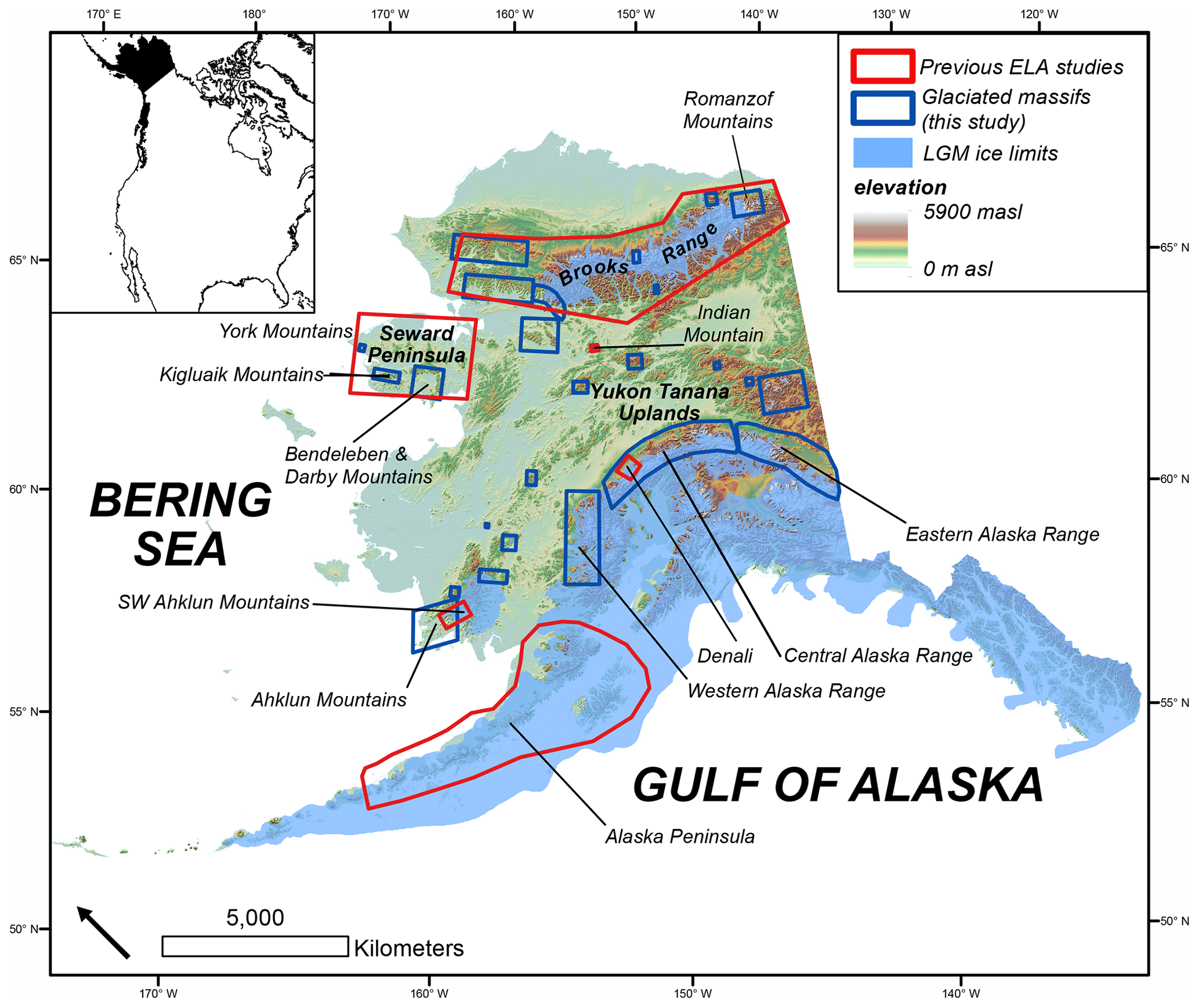
Figure 1 Map of Alaska with LGM ice limits (light blue; http://akatlas.geology.buffalo.edu/, last access: 4 January 2023; Kaufman et al., 2011). Glaciated massifs used in this study outlined in dark blue boxes. Previous studies highlighted, with reported LGM–contemporary ΔELAs in red: Brooks Range (Hamilton and Porter, 1975; Balascio et al., 2005), Seward Peninsula (Kaufman and Hopkins, 1986), Indian Mountain (Péwé, 1975), Denali (Dortch et al., 2010), SW Ahklun Mountains (Briner and Kaufman, 2000), and Alaska Peninsula (Mann and Peteet, 1994).

Pewé (1975) created a statewide compilation of LGM ELAs using the cirque floor elevation method, where the ELA is assumed to be the elevation of the floor of a cirque. This map revealed a clear west-to-east rise in ELAs across Alaska, which was later reinforced by subsequent studies from selected areas. In western Alaska, ELAs ranged from ∼ 350 to ∼ 600 m a.s.l. (Fig. 1; Balascio et al., 2005a; Briner and Kaufman, 2000; Kaufman and Hopkins, 1986). In central Alaska, LGM ELAs were higher, with values of 1530 ± 20 m a.s.l. on the Denali massif (Dortch et al., 2010). In eastern Alaska, LGM ELAs reached 1860 m a.s.l. (Balascio et al., 2005a). The LGM ELA gradient across Alaska outside of past Cordilleran Ice Sheet influence is hypothesized to have been due to a precipitation gradient similar to today's, with higher precipitation in western Alaska and lower precipitation in the eastern part of the state and the southern Bering Sea and the northernmost Pacific as the dominant moisture sources (Kienholz et al., 2015; Péwé, 1975).

However, there are two potential issues with these studies. First, the cirque floor elevation method of ELA calculation used by Pewé (1975) has since been suggested to represent a Quaternary average ELA rather than an LGM ELA, as these cirques are eroded across multiple glaciations and are therefore different than an LGM ELA (e.g., Mitchell and Humphries, 2015; Porter, 1989). Second, subsequent studies used a variety of ELA calculation methods, making the comparison of ELA results from region to region somewhat uncertain. Thus, statewide ELA calculations using updated congruent methods would improve knowledge of LGM ELA trends across Alaska.

Reconstructed LGM ΔELAs (LGM–contemporary ELA; see below) from these previous studies range from approximately −200 to −700 m in the Brooks and Alaska ranges, the Kigluaik and Ahklun mountains, and on Indian Mountain (Balascio et al., 2005a; Briner and Kaufman, 2000; Hamilton and Porter, 1975; Kaufman and Hopkins, 1986; Manley et al., 1997; Péwé, 1975). While these data all consistently highlight a key point – ELA lowering in Alaska during the LGM was less than the average global ca. −1000 m ELA depression – there are some features of previously published studies that we can now build on to create a more congruent dataset (Broecker and Denton, 1990; Nesje, 2014). First, past studies used different contemporary time periods to represent modern glacier ELAs (from different times in the 20th century) as reference points even as Alaskan glaciers were rapidly retreating (Zemp et al., 2019). Second, it is unlikely these modern glaciers were in equilibrium with climate due to this rapid retreat (Molnia, 2008). Third, different methods of ELA calculations of modern and paleoglaciers make direct comparisons more difficult. Fourth, the values from Pewé (1975) likely represent Quaternary average ELAs rather than LGM ELAs. These discrepancies open the door for a comprehensive study to standardize LGM ELA and LGM ΔELA reconstructions across Alaska.

We reconstruct paleoglacier surfaces for 480 independent LGM valley paleoglaciers, and do not include ice caps or large ice fields, such as the those that covered the Ahklun Mountains and the Brooks Range. To delineate the extent of LGM glaciers, we rely on decades of field mapping and chronology summarized in the Alaska PaleoGlacier Atlas (Kaufman et al., 2011). Indeed, there are clear distinctions both in the field and remote sensing data between LGM and pre-LGM deposits. We are therefore confident in LGM glacier outlines across Alaska for purposes of ELA reconstruction. While these glaciers may have reached their MIS 2 maxima asynchronously, available cosmogenic nuclide age constraints from moraine boulders (Fig. S2; Briner et al., 2005; Dortch et al., 2010; Matmon et al., 2010; Pendleton et al., 2015; Tulenko et al., 2018; Valentino et al., 2021; Young et al., 2009) and radiocarbon constraints (e.g., Child, 1995; Kaufman et al., 2003, 2012; Manley et al., 2001; Werner et al., 1993) indicate that this occurred within the timing of the LGM, further yielding credence to previous mapping.

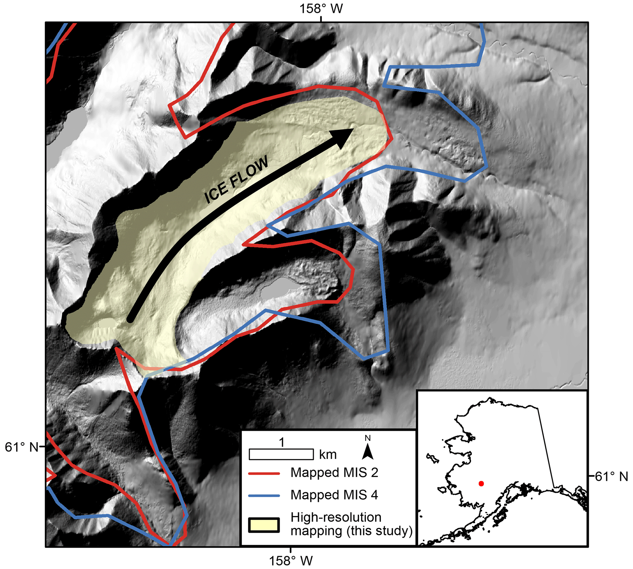
Figure 2 Hillshade image ($\mathrm{1}/\mathrm{3}$ arcsec [∼ 10 m] resolution DEM data from the USGS national map) of the eastern slope of the Chuilnuk Mountains, Alaska, showing previously mapped ice extents of the MIS 2 ice advance (red), MIS 4 advance (blue) from the Alaska PaleoGlacier Atlas v2 (Kaufman et al., 2011), and updated higher-resolution mapping from this study (yellow). Note that Kaufman et al. (2011) mapped ice limits at a 1:250 000 scale to capture statewide ice limits, and thus their limits are at a lower resolution. We used the lower-resolution polygons from the Alaska PaleoGlacier Atlas v2 as guides to ensure we mapped the correct MIS 2 ice extents.

Present-day and LIA glaciation in Alaska beyond areas once influenced by the Cordilleran Ice Sheet are limited (Millan et al., 2022; Molnia, 2008). These include glaciers in the Ahklun Mountains, the central Brooks Range, the northern and western Alaska Range, and a lone glacier in the Kigluaik Mountains. During the LIA (dated to the 19th century in Alaska; Barclay et al., 2009), Alaskan glaciers deposited well-defined moraine systems down valley of extant glacier systems that remain relatively unvegetated and sharp crested (Evison et al., 1996; Kathan, 2006; Molnia et al., 2008; Reinthaler and Paul, 2023; Sikorski et al., 2009). Thus, we can calculate ΔELAs (LGM_ELA–LIA_ELA) in valleys where simple LGM glaciers were independent from large ice caps or ice sheets, and within which there is clear geomorphic evidence of LIA glaciers. This precludes us from reconstructing ΔELAs, however, in valleys with LGM glaciers but lacking LIA glaciers or in valleys where there is evidence of LIA advances but the valley was covered by a large ice cap during the LGM, which we did not reconstruct (i.e., much of the central Brooks Range and Ahklun Mountains). Following these criteria results in few ΔELA calculations outside of the Alaska Range.

3 Methods

3.1 Datasets

We employed numerous datasets to calculate LGM and LIA ELAs and ΔELAs. First, we used the Alaska PaleoGlacier Atlas v2 to guide our mapping of LGM ice extents (http://akatlas.geology.buffalo.edu/, last access: 18 July 2023; Kaufman et al., 2011). In parts of the Brooks Range with limited Alaska PaleoGlacier Atlas v2 coverage, we relied on previous mapping by Balascio et al. (2005a). We used $\mathrm{1}/\mathrm{3}$ arcsec resolution digital elevation model (DEM) data from the United States Geological Survey (USGS) National Map (https://apps.nationalmap.gov/, last access: 19 July 2023). We used false color LANDSAT 8 imagery downloaded from the USGS Earth Explorer for LIA moraine mapping (https://earthexplorer.usgs.gov/, last access: 18 July 2023). Finally, we used modern ice thicknesses from Millan et al. (2022).

3.2 Paleoglacier reconstruction

We used the ArcGIS toolbox, GlaRe, in ArcMap 10.8 to recreate 480 LGM and 56 LIA glacier surfaces (Pellitero et al., 2016). We focused on independent valley glaciers for their simple geometry and relatively simple relationship between their size and climate (e.g., Oerlemans, 2005). We exclude ice caps and ice fields, such as those that covered the Brooks Range and the Ahklun Mountains, as GlaRe is not suited for such large and complex features, especially given inconsistent moraine preservation and a dearth of evidence on ice cap extent in some areas of the Brooks Range and Ahklun Mountains (Kaufman et al., 2011). Additionally, a lack of published data on paleo-ice divides, ice thicknesses, and bed topography for these ice caps hinders our ability to accurately reconstruct their surfaces and thus their ELAs. The GlaRe toolbox requires a terrain model of the paleoglacier bed, an outline of paleoglacier extent, glacier flowlines, and a user-defined basal shear stress. In valleys with extant glaciers, we created terrain models of paleoglacier beds by simply subtracting modern ice thickness maps from the DEMs (Millan et al., 2022). The Alaska PaleoGlacier Atlas v2 provides (Kaufman et al., 2011) shapefiles of glacier extents from different glaciations (i.e., MIS 2, MIS 4, and earlier) that are dated using available chronology, while Balascio et al. (2005a) provide paleoglacier information solely from the LGM. We used shapefiles of LGM paleoglaciers from the Alaska PaleoGlacier Atlas v2 (Kaufman et al., 2011) and glacier center coordinates from Balascio et al. (2005a) in the Brooks Range to roughly identify the extent of LGM paleoglaciers (Fig. 3; Kaufman et al., 2011). We then undertook more detailed mapping of LGM paleoglaciers based off these previously published extents (more detail was often necessary than that included in the Alaska PaleoGlacier Atlas) using well-established practices including identifying terminal and lateral moraine crests, trimlines, and cirque headwalls, to create higher-resolution shapefiles of LGM glacier extents (Fig. 3; e.g., Chandler et al., 2018). For large valley glaciers, we used watershed analyses in ArcMap to determine glacier multiple flowlines; for small cirque glaciers, we drew lines from the moraine directly to cirque headwall for simplicity. We calculated ice thickness every 25 m along these flowlines using GlaRe and a standard basal shear stress value of 100 kPa across all flow lines to ensure uniformity (Benn and Hulton, 2010; Pellitero et al., 2016). Using GlaRe, we reconstructed LGM glacier surfaces, using our “ice-corrected” bed DEMs where appropriate, paleoglacier extent, and flowline ice thickness data as inputs.

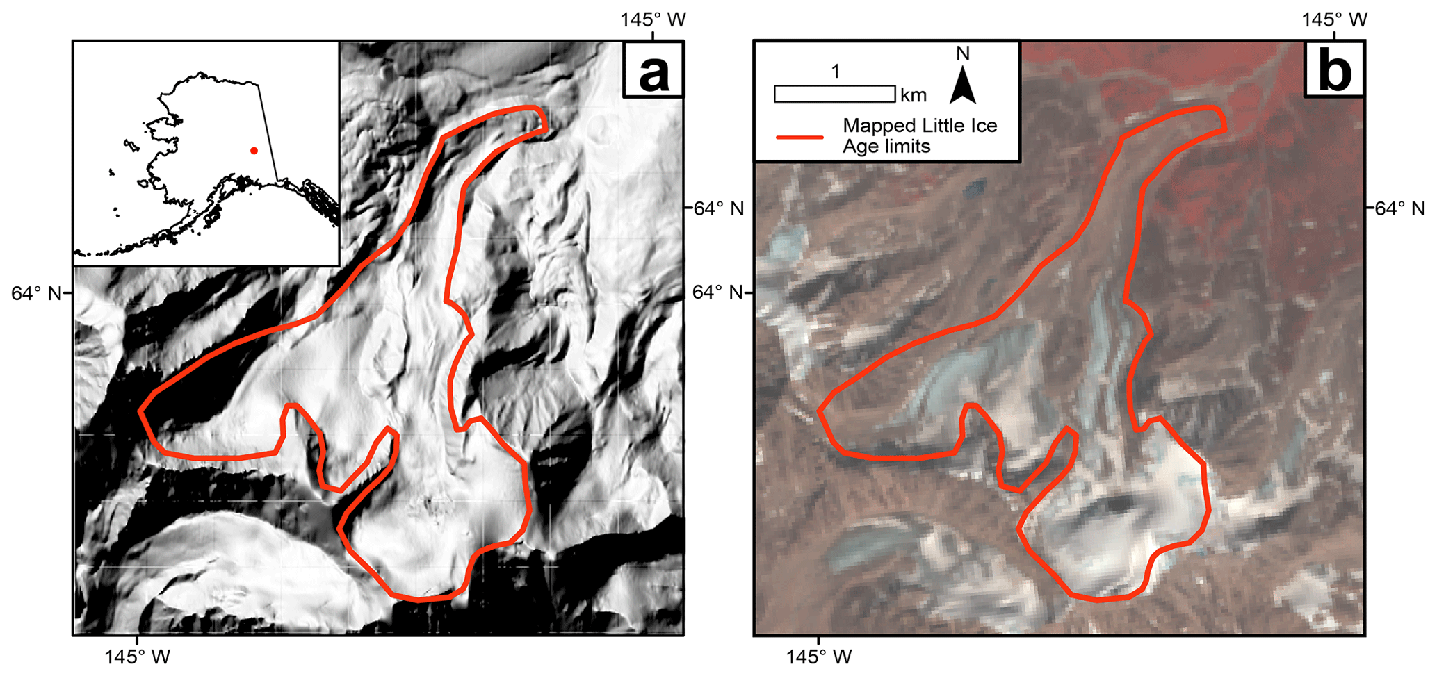
Figure 3 Representative hillshade (a) and LANDSAT8 false color images (b) from the eastern Alaska Range used for mapping Little Ice Age glacier extents. Note the sharp moraines in panel (a) and the clear transition from dark red (heavily vegetated) to brown-red in (b), both indicators of Little Ice Age moraines.

We repeated these steps for valleys with well-defined LIA glacier outlines, where we reconstructed independent LGM glaciers (i.e., not connected to ice caps in the Ahklun Mountains and Brooks Range) to allow for valley-scale LGM-to-LIA comparisons. Little Ice Age moraines in Alaska are defined by sharp, well-defined, vegetation-free crests (Molnia et al., 2008; Sikorski et al., 2009). In these locations, we used LANDSAT8 false color imagery to guide LIA moraine mapping by creating vegetation cover maps, which we used in tandem with our DEM data to identify LIA moraine crests (Fig. 3; Chandler et al., 2018; Reinthaler and Paul 2023). Based on Levy et al. (2004) and Sikorski et al. (2009), as well as our experience mapping former glaciers in Alaska, we have confidence in identifying the LIA moraine. In rare locations, pre-LIA moraines (Late Holocene moraines) may appear as fresh as LIA moraines, but in these cases the pre-LIA moraine crest is nested adjacent to LIA crests and would not result in a significantly different ELA if mistakenly outlined.

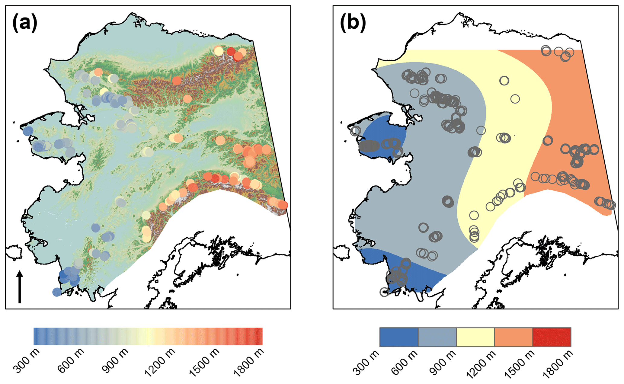
Figure 4 (a) AAR LGM ELAs for all 480 reconstructed LGM glaciers plotted on a color gradient. Blue are glaciers with lower ELAs; red, higher ELAs. Areas of Cordilleran Ice Sheet influence are excluded from the map. (b) Polynomial trend surface (third order) of LGM ELAs. Again, blue and red are low and high LGM ELAs, respectively.

3.3 Paleoglacier ELA and ΔELA calculation

There are many methods available to calculate paleoglacier ELAs (Pellitero et al., 2015). We chose two of the most widely used methods: the accumulation area ratio (AAR) and area–altitude balance ratio (AABR). The AAR is simply a ratio between the accumulation and ablation areas of a glacier; we employed a standard global ratio of 0.58 (Oien et al., 2021; Pellitero et al., 2015). For the AABR, a climatically controlled mass balance ratio is applied to glaciers in addition to the areas of the accumulation and ablation zones. The ELA calculated using the AABR is the altitude at which negative and positive mass balances are equal. We employ a ratio of 1.56, which a recent study has found to best represent glaciers worldwide, where there are no better available regional AABR values – this is true for Alaska today and during the LGM and LIA when the balance gradients are unknown (Oien et al., 2021). We calculated ELAs using LGM and LIA glacier surfaces as inputs to an ELA calculation toolbox in ArcMap (Pellitero et al., 2015). We applied previously published standard errors of 65.5 and 66.5 m for our AABR- and AAR-calculated ELAs, respectively, as provided by Oien et al. (2021). To calculate ΔELAs, we simply subtracted LIA ELAs from LGM ELAs on a valley-by-valley basis for valley systems that hosted glaciers during both periods; errors for these are 131 for AABR and 133 m for AAR to account for the maximum possible errors in ΔELA. In some instances, these errors lead to positive ΔELAs, but because LGM glaciers were more extensive than LIA glaciers, the positive ΔELAs indicated by the error are implausible. Thus, in these instances, we assume the maximum possible ΔELA is 0 m).

We created trend surfaces for LGM AAR and AABR ELAs across Alaska using the global polynomial tool in ArcMap with polynomial orders from 1 to 4. We also calculated root mean square and χ² statistics to help determine which polynomial trend surface best described regional ELA patterns. We excluded southern and southeastern Alaska from our reconstructed surfaces where we did not generate ELA data (Fig. 4)

3.4 Calculating LGM temperature depressions

We applied a range of plausible atmospheric lapse rates to our LGM–LIA ΔELAs to calculate LGM temperature depressions relative to the LIA following Eq. (1):

$$\begin{array}{}\text{(1)}& \mathrm{Temperature}\mathrm{depression}=\mathrm{\Delta }\mathrm{ELA}\times \mathrm{lapse}\mathrm{rate},\end{array}$$

where temperature depression is in ^∘C (and is negative), ΔELA is in kilometers, and lapse rate is in ^∘C km⁻¹. We used the maximum and minimum reported modern-day Alaskan lapse rates of 4.2 and 6.3 ^∘C km⁻¹ to calculate temperature depressions (Haugen et al., 1971; Verbyla and Kurkowski, 2019). We consider our calculated temperature depressions as maximum depressions because all available evidence suggests Alaska was drier during the LGM than today and during the pre-industrial (Bartlein et al., 2011; Dorfman et al., 2015; Finkenbinder et al., 2014, 2015; King et al., 2022; Löfverström and Liakka, 2016; Löfverström et al., 2014; Muhs et al., 2003; Tierney et al., 2020a, b; Viau et al., 2008). LGM lapse rates are unlikely to have been lower than modern lapse rates because drier air produces smaller-magnitude lapse rates because the lapse rate of an air mass increases as it loses its moisture through condensation. Therefore, we also calculated minimum temperature depressions using the dry adiabatic lapse rate of 9.8 ^∘C km⁻¹. The dry adiabatic lapse rate provides a maximum lapse rate for the atmosphere on anything but the shortest timescales (i.e., hours); therefore applying the dry adiabatic lapse rate to our ΔELAs provides a lower limit to our plausible LGM temperature depressions (Kaser and Osmaston, 2002).

4 Results

4.1 Last Glacial Maximum paleoglacier ELAs

Last Glacial Maximum paleoglacier ELAs calculated with AAR ranged from 293 ± 66.5 to 1745 ± 66.5 m a.s.l., while those calculated with AABR were between 306 ± 65.5 and 1742 ± 66.5 m a.s.l. (Fig. 4a). While the AAR and AABR vary slightly for the same paleoglaciers, these differences are small (12.5 ± 18 m; 1σ error reported throughout the article. We report AAR ELAs unless noted, as these calculations do not rely on knowledge of past mass balance gradients (which likely varied across Alaska during the LGM) as required for AABR.

The LGM ELAs values were lowest in the southwestern part of Alaska and highest in northeastern Alaska. In the Ahklun Mountains and surrounding massifs, ELAs were between 293 ± 66.5 and 754 ± 66.5 m a.s.l. Equilibrium line altitudes were also low on the Seward Peninsula (between 370 ± 66.5 and 910 ± 66.5 m a.s.l.) and in the western Brooks Range and its sub-ranges (472 ± 66.5 and 1028 ± 66.5 m a.s.l.). To the east, ELAs increased across the scattered massifs of the interior, reaching 858 ± 66.5 to 1271 ± 66.5 m a.s.l. Across the Alaska Range, LGM ELAs increased from 929 ± 66.5 m a.s.l. in the west to 1589 ± 66.5 m a.s.l. in the east. In the Yukon–Tanana Uplands, in eastern Alaska, ELAs were similar, between 1133 ± 66.5 and 1518 ± 66.5 m a.s.l. Finally, we report the highest ELAs in the northeastern Brooks Range, where they reached 1745 ± 66.5 m a.s.l.

4.2 Alaska LGM ELA trend surface

Our calculated LGM trend surface shows increasing ELAs from west to east (Fig. 4b); p tests applied to the data demonstrate a statistically significant correlation between longitude and LGM ELAs (p< 0.01; Fig. 5). However, we do not find significant correlation between latitude and LGM ELAs (Fig. S1 in the Supplement).

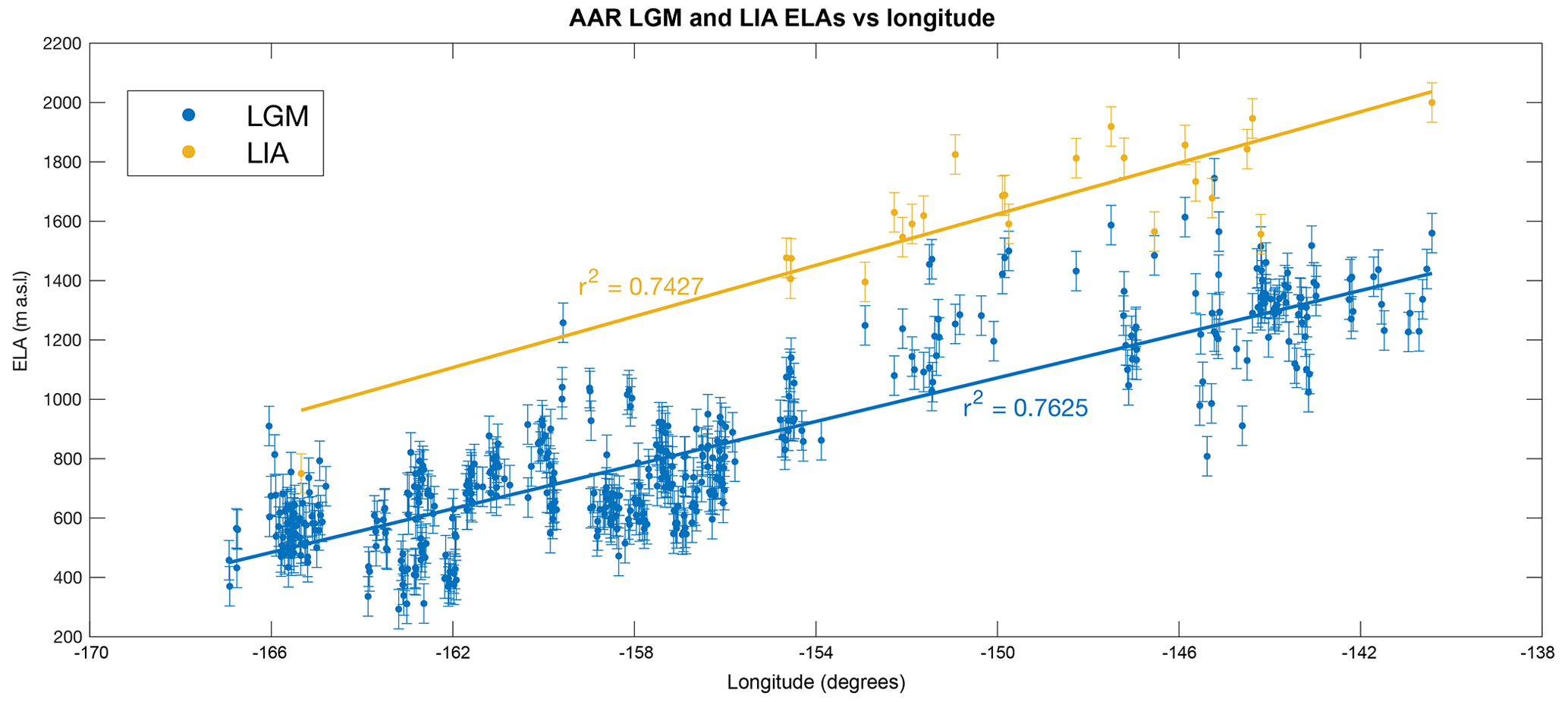
Figure 5 AAR LGM (blue) and LIA (yellow) ELAs plotted against longitude with lines of best fit.

4.3 LIA ELAs

We mapped 22 LIA glacier systems in the Alaska Range. We supplemented these data in valleys outside the Alaska Range that hosted both a simple LGM glacier and at least one LIA glacier. There were two valleys that met these criteria: one in the Kigluaik Mountains and one in the northeastern Brooks Range. Twelve of these 22 valley glacier systems in the Alaska Range hosted multiple LIA glaciers for every LGM glacier. For these systems, we report the mean of all LIA ELAs; these ranged from 1406 ± 66.5 to 1946 ± 66.5 m a.s.l. We calculated an ELA of 1950 ± 66.5 m a.s.l. for an LIA glacier on the western side of Mt. Osborn in the Kigluaik Mountains (Seward Peninsula). On the north slopes of Mt. Hubley in the Romanzof Mountains in the northeastern Brooks Range, we calculated an average LIA ELA of 1857 ± 66.5 m a.s.l. These LIA ELAs exhibit a similar trend to the LGM ELAs, with a statistically significant relationship between longitude and LIA ELA (p< 0.01; Fig. 5).

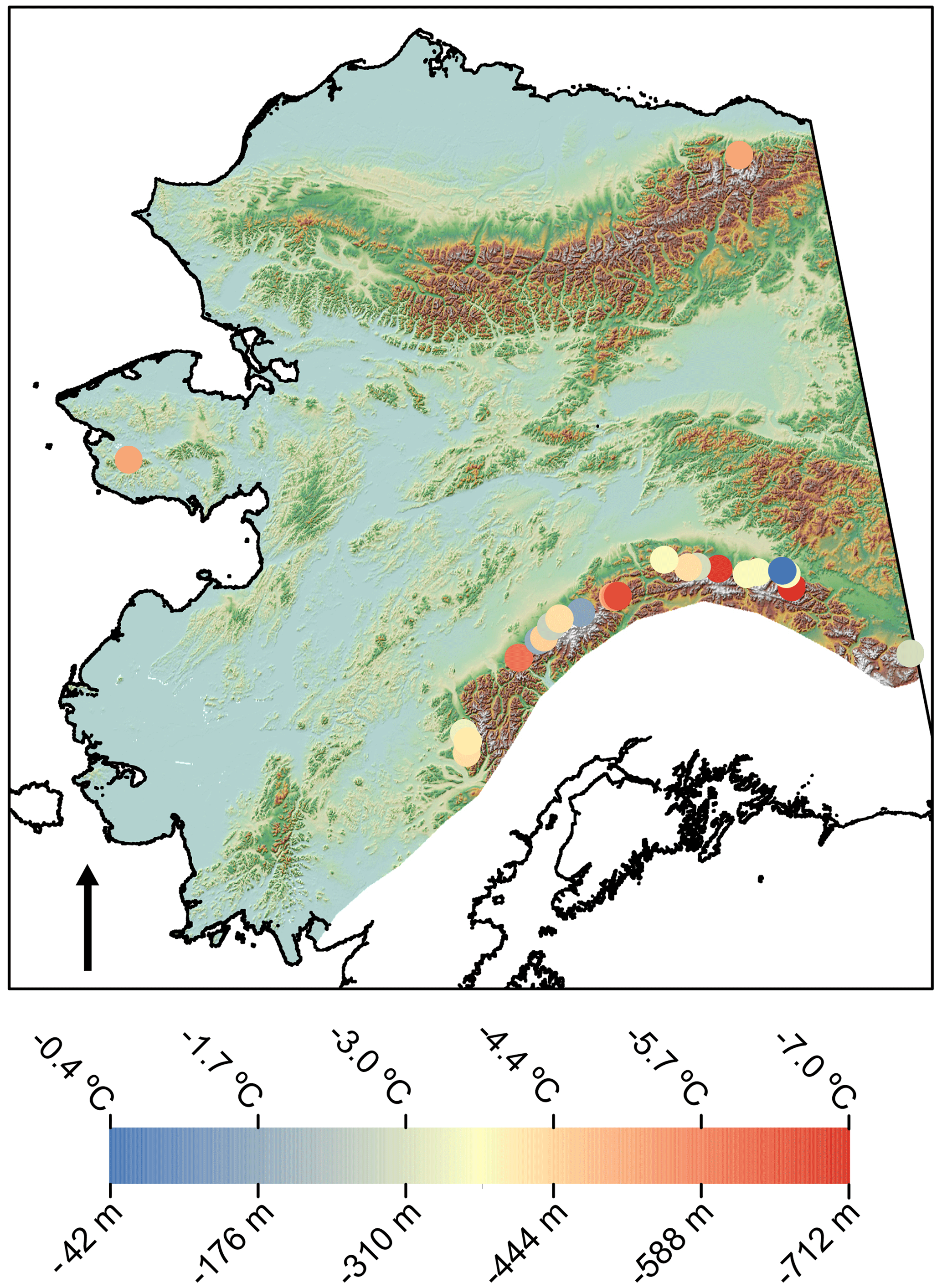
Figure 6 LGM–LIA ΔELAs and ΔELA-derived minimum summer temperature depressions calculated with the dry adiabatic lapse rate. Blue dots show little LGM ELA lowering (higher temperature depressions), while red dots show significant ELA lowering (lower temperature depressions). Areas of Cordilleran Ice Sheet influence are excluded from the map. Note that the lowest ΔELA is > −750 m.

4.4 LGM ΔELAs and summer temperature depressions

Last Glacial Maximum to Little Ice Age ΔELAs in the Alaska Range were between −42 ± 133 and −712 ± 133 m, with a median of −379 and a mean of −355 ± 180 m (Fig. 6). The ΔELA for our Brooks Range site was −243 m ± 133 and was −236 m ± 133 m in the Kigluaik Mountains. Median ΔELAs across our study areas were −335 m, with a mean ΔELA of −345 ± 177 m. We see no statistical relationship between longitude and ΔELA, though this may only reflect the Alaska Range due to limited data elsewhere in the state (Fig. S3).

Summer temperature depressions (n= 25) calculated with the lowest modern lapse rate estimate ranged between −0.2 ± 1.0 (positive temperature anomalies are implausible based on our methods as ΔELAs do not exceed 0 m) to −3.0 ± 0.6 ^∘C (median: −1.4 ^∘C; mean: −1.4 ± 0.8 ^∘C) across Alaska. These (n= 25) calculated with the highest modern lapse rate estimate range from −0.3 ± 1.4 to −4.5 ± 0.8 ^∘C (median: −2.1 ^∘C; mean: −2.2 ^∘C ± 1.1 ^∘C). Temperature depressions (n= 25) calculated with the dry adiabatic lapse rate range between −0.4 ± 2.2 and −7.0 ± 1.3 ^∘C (median: −3.3 ^∘C; mean: −3.4 ± 1.8 ^∘C).

5 Discussion

5.1 Comparisons with previous Last Glacial Maximum equilibrium line altitude reconstructions

Our calculated ELAs are generally consistent with those from previous studies. Our ELAs from across the Brooks Range broadly agree with those reported by Balascio et al. (2005a). Their study also reported a maximum Brooks Range ELA of 1860 m a.s.l. in the Romanzof Mountains, where we too calculated a range (and statewide) maximum ELA of 1745 ± 66.5 m a.s.l. On the Seward Peninsula, our ELAs are slightly higher than those previously reported (Kaufman and Hopkins, 1986). In the York Mountains, Kaufman and Hopkins (1986) calculated a single LGM ELA of 370 m a.s.l. – we present an average LGM ELA here of 477 ± 85 m a.s.l. (n= 5). In the Kigluaik Mountains, Kaufman and Hopkins (1986) reported LGM ELAs averaging to 470 m a.s.l. (n= 2), falling just outside 1σ of our mean LGM ELA for the Kigluaik Mountains of 585 ± 91 m (n= 64). However, their previously estimated average LGM ELA for the Bendeleben and Darby mountains of 630 m a.s.l. matches well with our mean LGM ELA of 657 ± 86 m a.s.l. These slight discrepancies in ELAs between the data are likely attributable to differences in ELA calculation; Kaufman and Hopkins (1986) used the toe-to-headwall area ratio method of ELA calculation using topographic maps, which has since been superseded by more robust ELA calculation techniques (Nesje, 2014).

Two previous studies in parts of the Ahklun Mountains report LGM ELAs of 390 ± 100 m a.s.l. and 540 ± 140 m a.s.l., both overlapping with our mean LGM ELA of 472 ± 117 m a.s.l. (Briner and Kaufman, 2000; Manley et al., 1997). Dortch et al. (2010) computed an average LGM ELA from the Peters and Muldrow glaciers near Denali in the central Alaska Range of 1530 ± 20 m a.s.l., which is a few hundred meters higher than our average ELA from the central Alaska Range of 1267 ± 145 m a.s.l.; this difference is likely attributable to different choices in AAR and AABR ratios, and not correcting for modern ice thickness in glacier surface reconstruction.

Though we did not calculate ELAs for the ice caps and ice fields over the Brooks Range and the Ahklun Mountains, it is unlikely that their ELAs would vary much from the surrounding independent valley glaciers. As the ELA of glaciers, including ice caps, are largely controlled by summer temperatures and annual precipitation, it holds that ice masses from similar locations should have similar ELAs. The ELA of large ice caps can vary across large geographic areas (e.g., Burgess and Sharp, 2004). Thus, we would expect the ELA of the Brooks Range ice cap, which stretched for ∼ 1000 km from west to east, to vary similarly to the ELAs of independent valley glaciers on the western and eastern edges of the range and not significantly influence our findings.

Our LIA ELAs are comparable to the limited published ELA data from Alaska. In several instances, others calculated LIA ELAs from valleys that were smothered by ice caps or ice sheets during the LGM, and thus we cannot make direct spatial (i.e., valley to valley) comparisons with our data (e.g., Daigle and Kaufman, 2009; Levy et al., 2004; Sikorski et al., 2009; Wiles et al., 1995). However, a study of LIA ELAs in the northeastern Brooks Range reported an average of 1977 ± 102 m a.s.l. (calculated with AAR of 0.58), within the error of our average LIA ELA from the same sub-range of 1857 ± 47 m a.s.l. (Sikorski et al., 2009).

We find that our average LGM–LIA ΔELA across all study sites of −355 ± 180 m and our LGM–LIA ΔELAs for individual mountain ranges generally match previously published ΔELAs (LGM–contemporary) from across the state, which ranged between −200 and −700 m (Balascio et al., 2005a; Briner and Kaufman, 2000; Dortch et al., 2010; Hamilton and Porter, 1975; Kaufman and Hopkins, 1986; Mann and Peteet, 1994; Péwé, 1975). Additionally, previously published LIA ELA reconstructions using similar AAR values from the Ahklun Mountains and central Brooks Range allow us to estimate range/sub-range average LGM–LIA ΔELAs when combined with our range/sub-range average LGM ELAs (Levy et al., 2004; Sikorski et al., 2009). These yield average LIA ΔELAs of −372 ± 117 m for the Ahklun Mountains and −249 ± 157 m for the central Brooks Range (errors from average LGM and LIA ELAs are summed). We note that these data do not reflect valley-scale changes in ELA but rather range-wide shifts. Thus, we do not calculate temperature depressions from these but provide them for ΔELA comparison purposes. Nevertheless, these previous data all fall within the range of our average statewide LGM–LIA ΔELA, and none approach the global average modern to LGM ΔELA of −1000 m. Though these previous studies that reported LGM ΔELAs (Balascio et al., 2005a; Briner and Kaufman, 2000; Dortch et al., 2010; Hamilton and Porter, 1975; Kaufman and Hopkins, 1986; Mann and Peteet, 1994; Péwé, 1975) exclusively used the contemporary modern ELA as a reference point for calculating ΔELAs and these glaciers may have been in states of disequilibrium, these still provide useful maximum LGM–LIA ΔELA constraints, as LIA ELAs would have been somewhat lower than those of modern glaciers given that LIA moraines are found outside the extents of extant glaciers. Indeed, the most recent studies indicate that maximum LIA lowering was between 22 and 83 m relative to modern across Alaska (Barclay et al., 2009; Daigle and Kaufman, 2009; Levy et al., 2004; McKay and Kaufman, 2009; Sikorski et al., 2009). Even when accounting for these LIA ELA depressions, our calculated LGM depressions do not approach the canonical global LGM–modern ΔELA of −1000 m.

We suggest the comparatively minor LGM–LIA ΔELAs in Alaska relative to the global average can be attributed to both increased aridity and relatively small summertime temperature depressions. As an example, the tropical Andes both hosted alpine glaciers and experienced conditions more arid today than during the LGM. Unlike Alaska, LGM–LIA ΔELAs here were near, or greater than, the global LGM–modern ΔELA (Rodbell, 1992; Stansell et al., 2007). Assuming no change in temperature from modern levels, drier LGM conditions suggest that LGM glaciers in the tropical Andes would have been smaller than today. However, these LGM glaciers were more extensive than modern due to high temperature depressions at high altitudes that allowed the glaciers to grow, such that their LGM–modern ΔELAs were near the global average (e.g., Rodbell, 1992; Stansell et al., 2007). Conversely, in Alaska, where the climate was also drier during the LGM than the LIA, low LGM–LIA ΔELAs are likely attributable to relatively low LGM temperature depressions. Last Glacial Maximum glaciers in Alaska were larger than the LIA, indicating some temperature depression, but unlike in the tropical Andes, this must have not been high enough to depress LGM ELAs by the global average of ∼ −1000 m. Indeed, LGM paleoclimate records of aridity and summer temperature from Alaska suggest conditions conducive to this: decreased annual precipitation and summers only slightly cooler than the LIA and much warmer than most of the high-latitude regions of the Northern Hemisphere.

5.2 ELA trends across Alaska

The gradient of LGM ELAs rising eastward agrees well with the previous statewide ELA reconstruction of Péwé (1975). Balascio et al. (2005a) also found a similar gradient in the Brooks Range, showing a clear rise in LGM ELAs from the west to the east. Studies from the Ahklun Mountains also reported a similar eastward rise in ELAs (Briner and Kaufman, 2000; Manley et al., 1997). The correlation between longitude and LIA ELA suggests that a similar gradient was present during both the LIA and LGM, with mountain ranges receiving less precipitation with increasing distance from the most probable moisture sources for our study areas in Alaska – the southern Bering Sea and northernmost Pacific Ocean. Precipitation from the Arctic Ocean was blocked by perennial sea ice during both the LGM and the LIA, and moisture moving northward from the Gulf of Alaska was influenced by the rain shadow created by the Cordilleran Ice Sheet and/or the southern flanks of Alaska Range, effectively eliminating other potential sources of precipitation for our study sites (Balascio et al., 2005a; Briner and Kaufman, 2008; Kienholz et al., 2015; Molnia, 2008; Péwé, 1975). Interestingly, these gradients persisted during periods when the Bering Strait was both open and closed, suggesting that prevailing moisture sources were not greatly impacted by the emergence of the Bering Land Bridge during the LGM. What remains unclear is if, and how, this LGM gradient would change with the inclusion of ELAs from south-central and southeastern Alaska. We might expect LGM ELAs to be lower here due to the proximity to the Pacific; however, the area was covered by the Cordilleran Ice Sheet until well after the LGM, and thus, we are unable to calculate ELAs here (Hamilton, 1994; Péwé, 1975; Walcott et al., 2022; Lesnek et al., 2018, 2020).

5.3 Records of LGM paleoclimate

For nearly a century, researchers have attributed the relatively limited LGM glaciation in Alaska to increased aridity and relatively warm temperatures, noting that Alaska was dissimilar to areas farther south that were completely covered by the Cordilleran and Laurentide ice sheets (Capps, 1932; Flint, 1943). This aridity has since been confirmed by numerous studies. A pollen record synthesis indicates Alaska received up to 125 mm less precipitation per year at 25 ka than at present and continued to receive reduced precipitation until 20 ka (Viau et al., 2008). Bartlein et al. (2011) synthesized pollen data and suggested LGM annual precipitation was ∼ 50 to ∼ 200 mm yr⁻¹ lower than at present. More recent pollen studies (not included in these syntheses) confirm this, with records from lakes in the Brooks Range and the Yukon–Tanana Uplands both indicating increased aridity in Alaska during the LGM (Finkenbinder et al., 2014; Abbott et al., 2010). Additionally, geochemical analyses of sediment from Burial Lake near the Brooks Range show high magnetic concentrations and a dearth of organic matter during the LGM, suggesting a dry, windy environment with increased amounts of aeolian material deposited (Dorfman et al., 2015; Finkenbinder et al., 2015). Investigation of the δ¹⁸O values from chironomids in the same sediments corroborate this, indicating a dry environment during the LGM (King et al., 2022). Finally, a lack of loess records across Alaska dating to the LGM is attributed to a dearth of vegetation to support loess deposition in turn caused by increased aridity statewide (Muhs et al., 2003).

A data assimilation product created with a collection of sea surface temperature data and an isotope-enabled climate model show annual precipitation differences of ca. −300 mm yr⁻¹ during the LGM relative to the pre-industrial period, corroborating paleoclimate records of aridity (Tierney et al., 2020a, b). Climate model results corroborate this, showing a range of pre-industrial to LGM annual precipitation deficits between −150 and −600 mm yr⁻¹ (Kageyama et al., 2021; Löfverström et al., 2014; Löfverström and Liakka, 2016). These proxy, data assimilation, and modeling studies justify our use of modern lapse rates and the dry adiabatic lapse rate to calculate a range of plausible LGM summertime temperature depressions. Because Alaska was drier during the LGM than today, the LGM environmental lapse rate is unlikely to have been smaller than the modern lapse rates nor would it exceed the dry adiabatic lapse rate for any significant period of time (i.e., maximum of hours; Kaser and Osmaston, 2002).

Last Glacial Maximum summer temperature records are sparse, yet those created through paleoclimate proxies, data assimilation, and models all suggest that summertime temperatures in Alaska were just a few degrees colder during the LGM than during the LIA or modern. Syntheses of pollen records show mean LGM summertime temperatures of between 2 and 5 ^∘C colder than today. (Viau et al., 2008; Bartlein et al., 2011). Similarly, chironomid-inferred summer temperature records from lakes in western Alaska yield LGM temperature reconstructions ca. −3.5 ^∘C below modern (Kurek et al., 2009). This is substantiated further by a leaf wax hydrogen isotope temperature reconstruction from the central Brooks Range indicating that LGM summers were ca. 3 ^∘C cooler than during the LIA (Daniels et al., 2021). Though these records represent small isolated geographic areas, their agreement substantiates only modest summer LGM temperature depression across Alaska.

Our relatively small summer temperature depressions are also corroborated by recent data assimilation studies. Tierney et al. (2020a) shows summer temperature depressions across our study area of ca. −3.6 ^∘C during the LGM, relative to the pre-industrial period (recalculated to match our study area; i.e., excluding southern Alaska). Despite this study leaning heavily on marine proxy data, their estimated LGM summer temperature depression for Alaska falls within our range of maximum summer temperature depressions of 3.4 ± 1.8 ^∘C.

Climate model results from a few studies vary, with some showing Alaska during the LGM being a few degrees warmer than during the pre-industrial (e.g., Otto-Bliesner et al., 2006) and others showing small LGM–LIA summer temperature depressions of −1 to −4 ^∘C (Löfverström et al., 2014; Löfverström and Liakka, 2016; Kageyama et al., 2021). These models indicate a clear pattern: Beringia was relatively warmer than other high-latitude northern areas, particularly the North Atlantic but perhaps even in northern Canada. Our data confirm this overall pattern of relatively warm summers in Beringia and highlight the veracity of models that simulate mild temperature depressions across Alaska.

Our paleotemperature data provide evidence of relatively mild LGM climate in Alaska, confirming climate model output and expanding information from the few sites with paleoclimate proxy data extending into the LGM. One may wish to consider whether the moraines from which we calculate LGM ELA values are all the same age. Although many LGM terminal moraines in the state remain undated, we compile available cosmogenic nuclide age constraints from moraine boulders (Fig. S2), which indicate that there is some variability in moraine age, but the dated moraines fall within the broad timing of the LGM. Furthermore, we suggest that the spread in moraine ages is likely related to small-scale oscillations of LGM glaciers during the LGM period instead of significant spatiotemporal differences in LGM climate across the state (Anderson et al., 2014). Thus, while we acknowledge that LGM moraine age may differ across the study area, we feel our ELA data still capture the LGM climate state.

Average summer global temperatures were ca. −6 ± 2.4 ^∘C lower during the LGM and were even lower in other parts of the high northern latitudes, including much of northern North America and the North Atlantic (Osman et al., 2021; Tierney et al., 2020a). Our range of ΔELA-derived LGM minimum summer temperature depression for Alaska of −3.4 ± 1.8 ^∘C, is similar to this global average but higher than some temperature depressions in the northern high latitudes (Tierney et al., 2020a). Similarly, a paleoclimate assimilation from the Intergovernmental Panel on Climate Change shows annual temperature depressions in parts of the Arctic similar to the global average, suggesting that Arctic cooling was not zonally homogenous during the LGM – both annually and in the summer (Forster et al., 2021).

5.4 Why was Alaska relatively dry and warm during the LGM?

Alaska was drier during the LGM than today, yet comparable LGM and LIA ELA gradients – at least across the Alaska Range – suggest similar moisture sources and highlight the importance of temperature as a control on glacier extent. The arid conditions in Alaska during the LGM have long been attributed to global eustatic sea level fall and the resultant emergence of the Bering Land Bridge, which has often been cited as a reason for relatively high LGM–modern ΔELAs in Alaska (Hopkins, 1982; Briner and Kaufman, 2008; Balascio et al., 2005a; Briner and Kaufman, 2000; Balascio et al., 2005b; Brigham-Grette, 2001; Elias et al., 1996). However, the similarity between LGM and LIA ELA gradients (i.e., with and without the presence of the Bering Land Bridge) suggests that the Bering Land Bridge did not play a major role in modulating precipitation during the LGM.

Syntheses of North Pacific sediment core records indicate lower sea surface temperatures during the end of the LGM (∼ 20 to ∼ 19 ka), suggesting low moisture availability (Praetorius et al., 2018, 2020; Davis et al., 2020; Caissie et al., 2010). Much of the Bering Sea, North Pacific, and Arctic Ocean was covered by perennial sea ice during the LGM, further inhibiting moisture availability and precipitation in Alaska, and thus leading to higher LGM–LIA ΔELAs there compared to the lower latitudes (Caissie et al., 2010; Pelto et al., 2018; Polyak et al., 2010, 2013; Sancetta et al., 1984). However, while the southern Bering Sea and northernmost Pacific was largely free of sea ice during the LIA, the Arctic Ocean was still covered by perennial sea ice. This led to similar precipitation gradients as the LGM, with the southern Bering Sea and northernmost Pacific as the primary sources of moisture.

Relatively low summer temperature depressions in Alaska are also likely responsible for the limited ELA lowering in Alaska during the LGM. While a complete and satisfying mechanism for relatively warm summer temperatures in Alaska remains elusive, a growing number of modeling studies indicate the possibility that disruptions to global atmospheric circulation caused by large LGM ice sheets may help explain this phenomenon. In short, persistent anticyclonic circulation over the large North American ice sheets has two mechanistic impacts on atmospheric circulation and the regional radiation budget over Alaska in model simulations: (i) jet stream circulation becomes more meridional and warm southerly surface air is persistently advected into Alaska (e.g., Roe and Lindzen, 2001; Löfverström et al., 2014) and (ii) atmospheric subsidence driven by anticyclonic circulation inhibits local cloud formation, increasing shortwave radiation in Alaska (e.g., Löfverström and Liakka, 2016; Löfverström et al., 2015). While model results are encouraging, the first mechanism is predominantly a wintertime phenomenon and cloud dynamics are often sources of biases in models (e.g., Bony and Dufresne, 2005), so further analyses are likely required to test the hypothesis that large North American ice sheets modulated summer temperatures in Alaska during the LGM. Additionally, Tulenko et al. (2020) investigated LGM glacier changes throughout North America and lent additional support for the limited extent of glaciers in Alaska during the LGM being related to ice-sheet-influenced circulation. Collectively, atmospheric circulation patterns, in combination with AMOC-influenced temperature depression in the North Atlantic sector, are a reasonable explanation for LGM temperature patterns around the high northern latitudes (Tulenko et al., 2020).

Because alpine glaciers are likely more sensitive to summer temperatures than to annual temperatures, we suggest that the limited extents of alpine glaciers in Alaska and their correspondingly low LGM–LIA ΔELAs were primarily due to relatively warm summers and influenced by reduced annual precipitation (Rupper and Roe, 2008; Tulenko et al., 2020). We posit that the gradient of LGM ELAs seen across the state is largely controlled by precipitation. The lack of a western (Bering Land Bridge instead of the Bering Sea) or northern (sea ice cover over Chukchi Sea) moisture source causes higher ELAs with increasing distance from the only available moisture source – the southern Bering Sea and northernmost Pacific. This gradient is especially pronounced in Alaska due to LGM aridity; though temperature is the main driver of these LGM ELAs, any precipitation would have undoubtedly played a key role in the growth of any glaciers.

6 Conclusions

• Minimum LGM–LIA ΔELA-based summer temperature reconstructions of −3.4 ± 1.8 ^∘C confirm recent marine proxy-based paleoclimate data assimilation studies that indicate Alaska experienced LGM temperature depressions similar to the global average. This contrasts with many of the high-latitude areas of the Northern Hemisphere, where temperature depressions were much lower. These data agree with proxy and model studies that show slightly cooler summer LGM conditions in Alaska. They also highlight that Alaska experienced relatively small summer LGM temperature depressions compared to other northern high-latitude areas, suggesting that Arctic summertime cooling was not latitudinally congruent.

• LGM and LIA ELA reconstructions demonstrate similar gradients and statistically significant relationships between longitude and climate, indicating the influence of precipitation on glacier extent. The similarity of the gradient also suggests a similar moisture source during both the LGM and LIA and the lack of influence from the Bering Land Bridge.

• Future work should focus on modeling LGM glaciers in Alaska to supplement ELA-based paleoclimate records, calculating hypothetical modern or LIA ELAs to calculate ΔELAs and temperature depressions statewide, and on deriving ELAs and ΔELAs across the rest of Beringia (i.e., eastern Siberia) to assess paleoclimate conditions more broadly.