the Creative Commons Attribution 4.0 License.
the Creative Commons Attribution 4.0 License.
 | 08 Feb 2024
Effective diffusivity of sulfuric acid in Antarctic ice cores
Raphael Sauvage
Linh Vu
Benjamin H. Hills
Mirko Severi
Edwin D. Waddington
Deposition of sulfuric acid in ice cores is important both for understanding past volcanic activity and for synchronizing ice core timescales. Sulfuric acid has a low eutectic point, so it can potentially exist in liquid at grain boundaries and veins, accelerating chemical diffusion. A high effective diffusivity would allow post-depositional diffusion to obscure the climate history and the peak matching among older portions of ice cores. Here, we use records of sulfate from the European Project of Ice Coring in Antarctica (EPICA) Dome C (EDC) ice core to estimate the effective diffusivity of sulfuric acid in ice. We focus on EDC because multiple glacial–interglacial cycles are preserved, allowing analysis for long timescales and deposition in similar climates. We calculate the mean concentration gradient and the width of prominent volcanic events, and analyze the evolution of each with depth and age. We find the effective diffusivities for interglacial and glacial maximums to be m2 a−1, an order of magnitude lower than a previous estimate derived from the Holocene portion of EDC (Barnes et al., 2003). The effective diffusivity may be even smaller if the bias from artificial smoothing from the sampling is accounted for. Effective diffusivity is not obviously affected by the ice temperature until about −10 ∘C, 3000 m depth, which is also where anomalous sulfate peaks begin to be observed (Traversi et al., 2009). Low effective diffusivity suggests that sulfuric acid is not readily diffusing in liquid-like veins in the upper portions of the Antarctic Ice Sheet and that records may be preserved in deep, old ice if the ice temperature remains well below the pressure melting point.
- Article
(2175 KB) - Full-text XML
- BibTeX
- EndNote


Ice cores preserve unique records of past climate (e.g., EPICA, 2004; NEEM, 2013; WDPM, 2013). Interpreting the records requires knowledge of any post-depositional alteration, such that the quantity measured in ice that was deposited in the past can be interpreted as what was deposited at the surface of the ice sheet at that time (e.g., Cuffey and Steig, 1998; Pasteur and Mulvaney, 2000; Bereiter et al., 2014). In general, ice cores are excellent at preserving records because of the cold temperatures and the lack of processes that might disturb the record. Many records – water isotopes and chemical compounds – undergo some amount of post-depositional alteration in the near-surface snow, firn column, or solid ice (e.g., Dibb et al., 1998; Johnsen et al., 2000; Aydin et al., 2014; Osman et al., 2017). In the case of post-depositional diffusion of water isotopes, the amount of diffusion can be estimated and used for paleoclimate reconstruction (Gkinis et al., 2014; Kahle et al., 2021); however, for most soluble impurities and atmospheric gases, the primary goal of understanding post-depositional processes is to ensure accurate reconstructions.
Here we investigate the diffusivity of sulfuric acid using a record of sulfate from the European Project of Ice Coring in Antarctica (EPICA) Dome C (EDC) ice core (Severi et al., 2007). We focus on sulfate for the following two reasons: (1) the deposition of sulfate from volcanic events provides distinct features to identify and assess the change in shape with depth/age and (2) the importance of volcanic matching in synchronizing timescales (e.g., Ruth et al., 2007; Severi et al., 2007; Fujita et al., 2015; Buizert et al., 2018; Winski et al., 2019; Svensson et al., 2013, 2020; Sigl et al., 2013, 2015, 2022). Stable soluble impurities, such as sulfate, can remain as distinct layers in deep ice cores (e.g., Zielinski et al., 1997; Fujita et al., 2015); however, chemical peaks due to post-depositional alteration in deep, and warm, ice have also been identified (e.g., Traversi et al., 2009; Tison et al., 2015). Sulfuric acid has a eutectic temperature of −75 ∘C, such that if it is present at the grain boundaries and triple junctions, a liquid vein network may exist, even in the cold near-surface ice of the East Antarctic plateau (Dash et al., 2006). Some studies indicate that sulfuric acid is located at the triple junctions (Fukazawa et al., 1998; Mulvaney et al., 1988), particularly in specimens with high concentrations of sulfate (Barnes and Wolff, 2004), although there are questions about whether the sample preparation caused the sulfuric acid to concentrate there. The sulfate may be in the form of salt micro-inclusions in grains (Ohno et al., 2005), which would reduce the mobility in ice; however, sulfuric acid dominates the sulfate budget (Legrand, 1995), and we therefore use sulfate as an indicator of sulfuric acid. Thus, whether sulfuric acid is primarily located at the veins, grain boundaries, or within the ice lattice remains an open question, and the mechanisms driving diffusion are uncertain.
Addressing the diffusion of sulfate in veins, Rempel et al. (2001) showed that impurity fluctuations may retain their amplitude but migrate towards warmer temperatures and away from the ice the impurity was deposited with; however, Ng (2021) showed that including the Gibbs–Thompson effect due to the grain curvature may cause these peaks to diffuse rapidly and therefore not retain their amplitude or migrate. The sulfate and electrical conductivity measurements (ECMs) of Antarctic ice cores also show reduced amplitude (Barnes et al., 2003, hereafter B03; Fujita et al., 2015; Fudge et al., 2016) in older ice. B03 found an effective diffusivity of sulfate to be m2 a−1 at −53 ∘C for Holocene ice at EPICA Dome C (EDC), which is 2 orders of magnitude greater than the self-diffusion of ice at −53 ∘C ( m2 a−1), which they considered an upper limit for the diffusivity of sulfate in the ice lattice. They proposed two mechanisms of connected and unconnected vein networks to explain the effective diffusivity. Fudge et al. (2016) estimated an effective diffusivity of m2 a−1 at −30 ∘C at the West Antarctic Ice Sheet Divide (WDC), which has a smaller value despite a warmer temperature.
Here we assess the effective diffusivity of sulfate at EDC with two methods. First, we follow B03 in calculating the scaled mean gradient. We extend their analysis to the full depth of the EDC ice core. We focus on only the interglacial and glacial maximum time periods to reduce the influence of the climate at the time of deposition. Second, we identify the widths of volcanic peaks throughout the core and evaluate the widening of them with a numerical diffusion model.
2.1 EDC sulfate data set
The sulfate record for EDC was measured with fast ion chromatography (Traversi et al., 2009; Severi et al., 2015). The sampling resolution is approximately 4 cm in the Holocene and increases to approximately 2 cm by 44 ka, where it remains for the rest of the core. The EDC sulfate record has been widely used for volcanic matching (e.g., Severi et al., 2007, 2012; Buizert et al., 2018) and calculating volcanic forcing (e.g., Sigl et al., 2015, 2022). We assume that vertical variations in the sulfate record greatly exceed lateral variations, such that the diffusion can be treated as a one-dimensional problem.
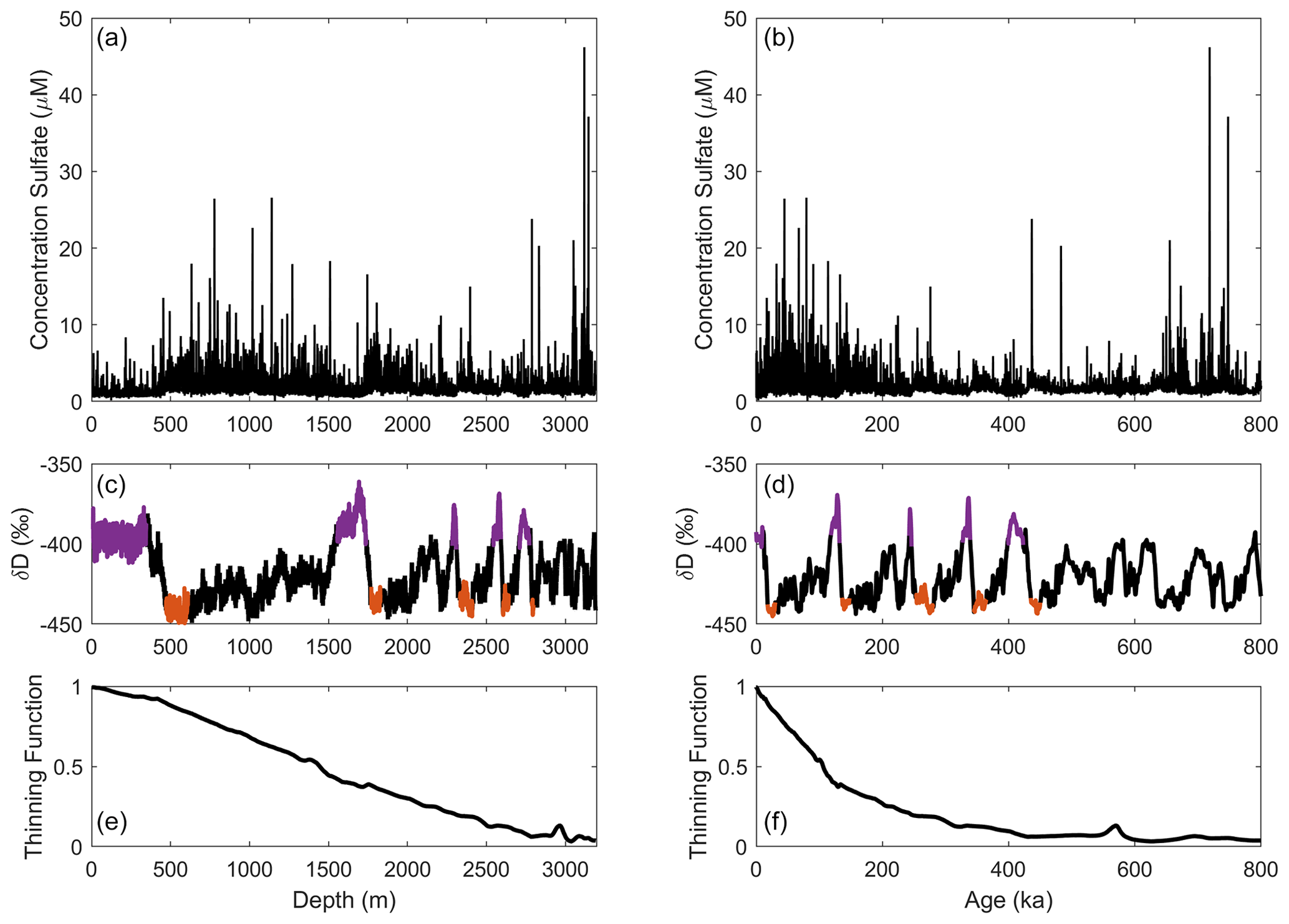
Figure 1Sulfate (a, b; Traversi et al., 2009; Severi et al., 2015), deuterium (c, d; EPICA, 2004), and the thinning function (e, f) plotted by depth (a, c, e) and age (b, d, f) on the Antarctic Ice Core Chronology 2012 (Bazin et al., 2013; Veres et al., 2013). The most recent five interglacials are plotted in purple, and glacial maximums are plotted in orange on the deuterium plots (c, d). Earlier interglacials do not reach the warm levels of most recent five.
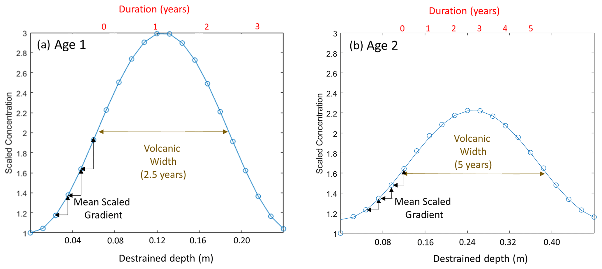
Figure 2Schematic illustration of the evolution of a volcanic peak from an initial profile (a) to a profile after diffusion has occurred (b). The mean scaled gradient is illustrated in black. The volcanic width method (Sect. 2.3) is in brown. Note that the x axis is destrained depth and is a different scale in panels (a) and (b).
2.2 Scaled mean gradient
Diffusion will reduce the amplitude of variations and broaden peaks in the sulfate record. To calculate the effective diffusivity, we first need a quantitative measure of the sulfate variability and then we need an expression for inferring the effective diffusivity from the change in the sulfate variability. One method for calculating the variability uses the difference between successive points over fixed depth intervals (Fig. 2). The mean difference between successive points will decrease more quickly with age for greater effective diffusivities. This technique has the advantage of using all the available data in a section of interest and was first described by B03. In B03, this mean difference was termed the scaled mean gradient. As the name scaled mean gradient suggests, B03 took the additional step of scaling the sulfate data to account for variations due to the climate at deposition. B03 investigated only the Holocene data. When we extended the analysis to glacial climates, we found that the scaling did not account for differences between different climates at deposition. We therefore decided to only compare similar climate states, namely the interglacials to interglacials and the glacial maximum periods to glacial maximums. We also found that the inference of effective diffusivity was not sensitive to whether we scaled the data or left it unscaled. We use the scaling, as described by B03, to be consistent with previous results. Below we focus on two primary equations – for the scaled mean gradient and for the effective diffusivity – and provide the supporting equations to explain the calculations performed. A full description can be found in B03.
The first primary equation is for calculating the scaled mean gradient (B03; Eq. 1), which is an estimate of
where c′ is the scaled sulfate profile, z is the destrained depth, Δz is a fixed depth interval (10 m), and δc′(z) is the difference between successive points. The sulfate profile is scaled to account for differences in the amplitude of variations caused by variations in climate rather than due to diffusion, as follows:
where c0 is calculated as the intercept of the total area under the peaks plotted against the mean concentration. We perform the scaling to be consistent with the B03 methodology.
The second primary equation finds the effective diffusivity using the scaled mean gradient (B03; Eq. 9), as follows:
where Deff is the effective diffusion coefficient in solid ice, k is the wave number (defined in Eq. 7), t is time, and m0 is the initial scaled mean gradient. This equation is derived by noting that sulfate concentration varies primarily with depth, such that horizontal variations can be neglected, yielding a one-dimensional process in depth as follows:
where χ(t) accounts for the vertical thinning, including the densification of firn. This differential equation can be solved, following Johnsen et al. (2000), by relating a diffusion length, l, to Deff(t) as follows:
where is the vertical strain rate. Here, we first destrain the ice based on the thinning function of the Antarctic Ice Core Chronology 2012 (AICC2012; Bazin et al., 2013; Veres et al., 2013), such that has been removed. The amplitude can then be defined in relation to the initial amplitude, as calculated for the Holocene and Last Glacial Maximum (LGM); age durations for intervals are given in Appendix A. Assuming a harmonic cycle with a wave number, k
where H is the amplitude after some time, and H0 is the initial amplitude. The wave number, k, is related to the mean peak width
where is the mean peak width for the full Holocene or LGM profile and can be calculated from the mean absolute gradient as
where is the mean absolute gradient, and ztotal is the full depth for either the Holocene or LGM.
2.3 Width of volcanic peaks and numerical modeling of diffusion
An alternate technique for measuring the evolution of chemical signals is to identify individual volcanic peaks (e.g., Fudge et al., 2016; Fig. 2). We identified peaks based on their prominence; i.e., the amplitude between the peak and the nearest local minimum in both up- and down-core directions with the findpeaks function in MATLAB. Finding the prominence allows a standardized approach that accounts for different background levels of sulfate deposition that occur in different climate states. Our approach compared well with studies that used an exceedance of the median absolute deviation (Traufetter et al., 2004; Sigl et al., 2015; Nardin et al., 2020; Cole-Dai et al., 2021) in sliding windows.
The volcanic events were identified in age on the AICC2012 timescale (Bazin et al., 2013; Veres et al., 2013). The findpeaks algorithm calculates the width of the peak at the half-maximum of the sulfate peak amplitude. The width is in years and can be converted to depth using the depth–age relationship. As for the scaled mean gradient, we compare the interglacial and glacial maximum periods separately. For each period, we use the largest 25 events. We primarily consider the median widths for each period to reduce the influence of either exceptional volcanic events or anomalous sulfate peaks. The anomalous peaks begin primarily below 2800 m (Traversi et al., 2009) but may begin around 2500 m depth (Wolff et al., 2023). The anomalous sulfate peaks are discussed further in Sect. 4.1.
The effect of diffusion is modeled with a one-dimensional numerical model (e.g., Eq. 4). The model, described in Fudge et al. (2016), evolves an initial peak through time based on the effective diffusivity and the vertical thinning. At each time step, the diffusion is calculated first, and then the ice is thinned. The amount of thinning at each time step is calculated from the thinning function (Veres et al., 2013; Bazin et al., 2013). The ice temperature and effective diffusivity can be varied at each time step, although we only show results using a constant effective diffusivity here. We model the evolution of a Gaussian peak. The initial width of the peak is determined by the sulfate data in the Holocene (0.128 m) and LGM (0.135 m). The initial thicknesses are similar but, because the accumulation rate in the LGM is a factor of 2 lower, the duration of the events is twice as long in the LGM. The amplitude of the peak is 3 times the background concentration, although in practice the amplitude is not critical because we calculate the relative change. The peak width is computed as the width at the half-maximum amplitude, which is the same method as used on the sulfate data.
2.4 Estimating bias by artificial smoothing
The calculation of effective diffusivity may be affected by a bias due to artificial smoothing. The sampling resolution in depth for the sulfate record is approximately 4 cm for the first 45 ka and 2 cm for older ages. The increasing thinning with depth results in each measurement averaging over a longer duration, which can artificially smooth the mean gradient by failing to fully resolve peaks and troughs. If the sampling resolution is short relative to the signal, such as a multi-year volcanic event with seasonal sampling, then the artificial smoothing will be negligible. On the other hand, if the sampling resolution is long relative to the signal, then significant smoothing will occur.
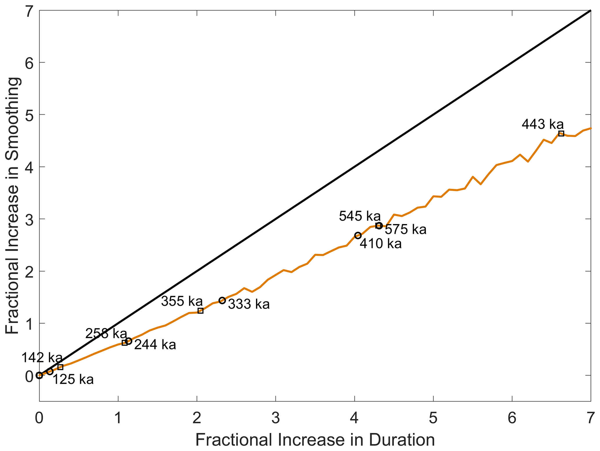
Figure 3Estimate of the impact of artificial smoothing due to sample size in each interglacial or glacial maximum period. The amount of artificial smoothing (brown) increases more slowly than the increase in the average sample duration. The one-to-one line is shown in black.
We estimate the amount of artificial smoothing for older ice by resampling the Holocene data. We select the period 2.3 to 11.3 ka, which has relatively even sampling durations and is well resolved due to the small amount of vertical thinning. We resample the data at increasing durations and compare the mean gradients of the resampled data with the mean gradient of the original data. The ratio of the original mean gradient to the resampled mean gradient is the size of the correction that should be applied (Fig. 3). The amount of artificial smoothing increases at about 70 % of the rate of the increase in duration.
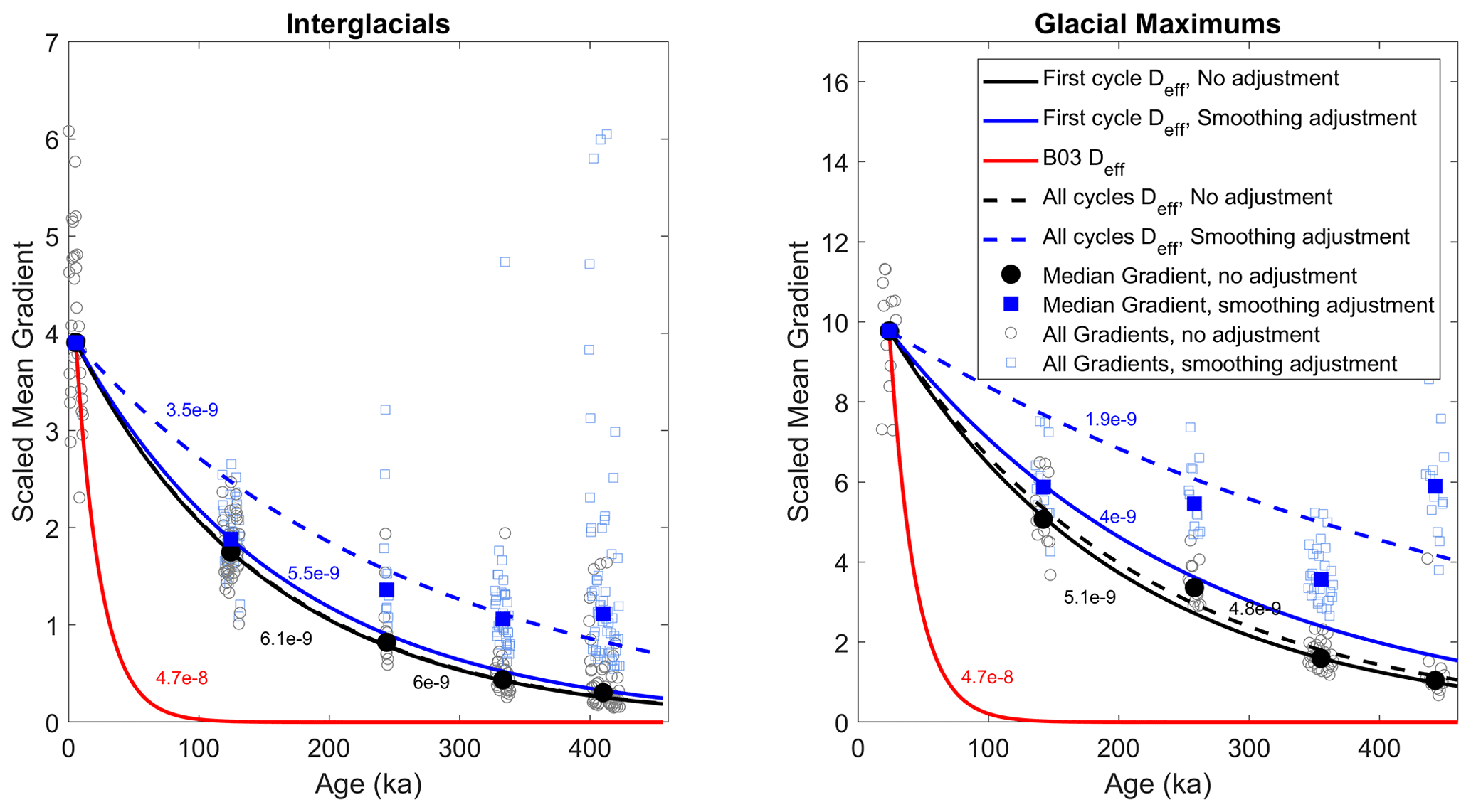
Figure 4The effective diffusivity, Deff (labeled in units of m2 a−1), for the different inferences from the scaled mean gradients in interglacial and glacial maximum periods. Scaled mean gradients for 10 m sections are shown by open symbols; the median scaled mean gradients for each interglacial or glacial maximum are shown by solid symbols. Solid lines show the inference of effective diffusivity from the first glacial cycle; dashed lines are adjusted for artificial smoothing. Black lines and symbols have no adjustment for artificial smoothing; blue lines and symbols are adjusted for artificial smoothing. The red line is the previous estimate of effective diffusivity from B03, using Holocene data.
The potential bias due to artificial smoothing for each interglacial and glacial maximum periods is shown in Fig. 4. The Last Interglacial–Glacial (LIG) period and Penultimate Glacial Maximum (PGM) sampling interval is 2 cm, approximately half that of the Holocene and LGM, such that the shorter sampling interval largely offsets the layer thinning. For older ages, the artificial smoothing becomes larger, reaching a maximum of 440 % for the glacial period centered at 443 ka (Marine Isotope Stage 12). This is an outlier, due to the small annual layer thickness during that period, but highlights that the correction for artificial smoothing becomes quite large and potentially dominates the estimate of effective diffusivity.
3.1 Effective diffusivity from the scaled mean gradient
The characteristics of the sulfate record vary with the climate state at deposition. The sulfate deposited in interglacials has a lower concentration than during the glacial periods. This is most evident in Fig. 1a, where the increase in sulfate concentration is visible at about 450 m. Comparing the sulfate gradients among different climate states is problematic. We found that scaling the mean gradients did not fully remove the differences due to the climate at deposition (Sect. 2.1). Therefore, we compare the sulfate gradients among periods with similar climate characteristics, specifically the interglacial periods and the glacial maximum periods separately.
We follow the methods of B03 (Sect. 2.2) and repeat the calculations for the initial sulfate parameters for the Holocene (0–11.3 ka). We find c0 is 0.62 compared to the B03 value of 0.54 and the same value for of 0.19 m. The small difference is likely due to updates in the sulfate data set and thinning function. We also find initial parameters for the LGM (18–30 ka). For both the Holocene and LGM, we assume that these initial values at deposition were the same for previous interglacial and glacial maximum periods (Table 1).
Table 1Effective diffusivities calculated between the Holocene and the Last Interglacial and the Last Glacial Maximum and the Penultimate Glacial Maximum.
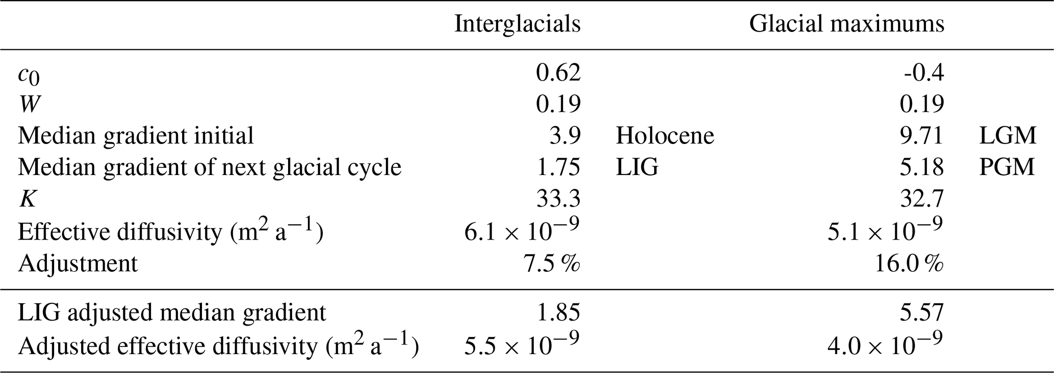
We first calculate the effective diffusivity in the Holocene to directly compare with B03. We find an effective diffusivity of m2 a−1, approximately 15 % greater than the B03 value of m2 a−1. Like the small difference in the c0 value, the larger effective diffusivity is likely due to revisions in the sulfate data set and thinning function. As shown below, a 15 % difference is small compared to the difference in the inferred effective diffusivity when using data older than the Holocene.
We next calculate the effective diffusivity using the most recent glacial cycle by comparing the Holocene and LIG and the LGM and PGM. This allows a much longer time period for diffusion to operate. The difference between the interglacial and glacial maximums of the most recent cycle provide a useful duration (∼120 ka) for diffusion to have operated without the ice having become too greatly thinned. In addition, the sample resolution in depth was smaller for the older periods, which yielded a relatively small increase in the duration (age span) of each sample compared to the most recent periods (Sect. 2.4).
We use Eq. (3) to calculate the effective diffusivity, where mz is the median scaled mean gradient of the LIG or PGM, and m0 is the median scaled mean gradient of the Holocene or LGM. The value of k is calculated from the Holocene or LGM data. The resulting effective diffusivities are m2 a−1 (Table 1), using the interglacials, and m2 a−1, using the glacial maximums.
For the LIG, we can calculate an effective diffusivity corrected for artificial smoothing by increasing the mean absolute gradient by the 7.5 % calculated above; this decreases the effective diffusivity to m2 a−1. For the PGM, the 16 % adjustment for artificial smoothing results in a decrease in the effective diffusivity to m2 a−1. The calculated effective diffusivities are shown in Table 1 and Fig. 4.
Table 2Effective diffusivity values (Deff; in units of 10−9 m2 a−1) for interglacial and glacial maximum periods. Italics indicate two outliers which help define the lower bound.
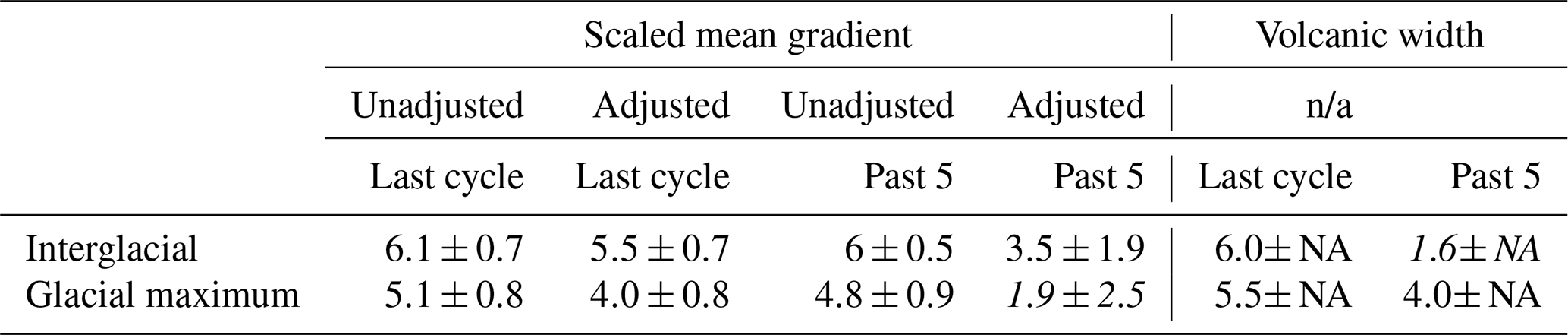
Note: n/a is for not applicable; NA is for not available
The scaled mean gradients from the past five glacial cycles can also be used to estimate the effective diffusivity. We perform a linear fit to the log of the medians for each period for both the unadjusted and adjusted values (Fig. 4; Table 2); we fit the medians instead of all the points to account for the different number of points in each interglacial. The fit for the past five glacial cycles finds similar effective diffusivities for the unadjusted values for both the interglacial and glacial maximum periods; however, the fit finds significantly smaller effective diffusivities for the adjusted values. The inferred interglacial effective diffusivity is approximately 40 % smaller than that inferred for the Holocene–LIG, while the glacial maximum value is approximately 55 % smaller.
For both the most recent glacial cycle and the past five glacial cycles, we calculate the uncertainty in the effective diffusivity based on the 95 % confidence interval of the linear fit to the log of the scaled mean gradients; instead of using the medians, we use the individual data points. We report this as an approximate value by taking the 95 % confidence range and dividing by two. The uncertainties are given in Table 2.
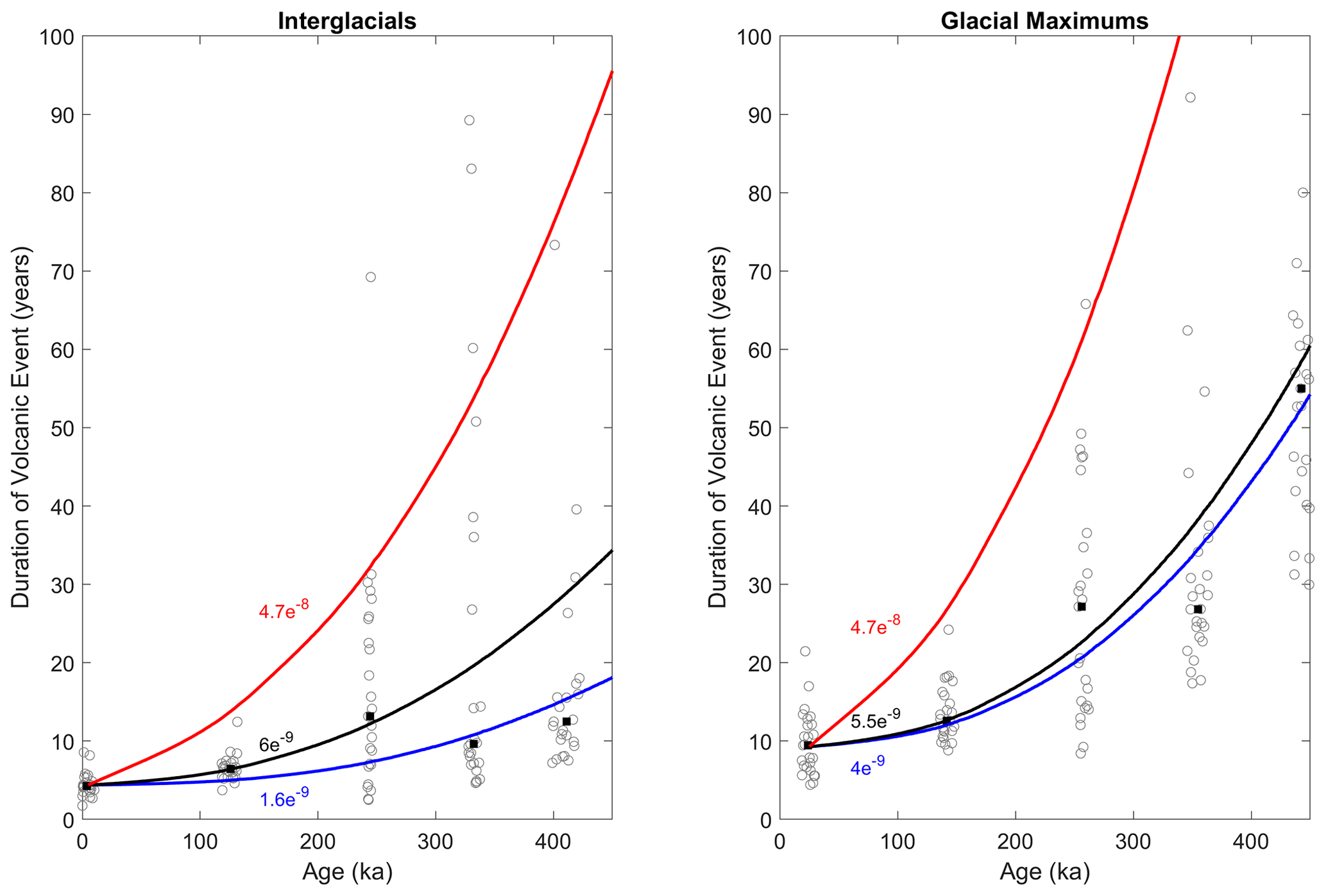
Figure 5Duration of the 25 largest volcanic events (gray circles) for each interglacial and glacial maximum period. Medians for each period are shown as black squares. Solid lines are the modeled volcanic event durations using constant effective diffusivities. Black lines are the best fit to the Holocene–LIG or LGM–PGM. Blue lines are best fit to all five interglacial or glacial maximum periods. Red is the B03 estimate from Holocene data.
3.2 Effective diffusivity using widths of volcanic events
The duration of the 25 largest volcanic events, and their medians, for the interglacial and glacial maximums of the past five glacial cycles is shown in Fig. 5. The duration of the largest events increases with age, although there is a lot of scatter. The median duration of a volcanic event in an interglacial increases relatively little from about 5 years in the Holocene to about 10 years for interglacials older than 200 ka. The glacial maximums, in contrast, show a large increase in duration, from 10 years in the LGM to over 50 years at ∼450 ka. The widths of the largest volcanic events are less sensitive to artificial smoothing due to the sample duration than the scaled mean gradient because the volcanic signal is long relative to the sampling interval; therefore, we do not add a correction for artificial smoothing (Sect. 2.4).
The numeric model (Sect. 2.3) is used to infer the effective diffusivity by minimizing the misfit to the median widths of each period. As with the scaled mean gradients, we infer a constant effective diffusivity and start with only the most recent glacial cycle. For the LIG–Holocene, an effective diffusivity of m2 a−1 is the best fit; for the LGM–PGM, the best fit is m2 a−1. The best fits for all five glacial cycles are m2 a−1 for the interglacial periods and m2 a−1 for the glacial maximums. We do not calculate an uncertainty for the inferences and will discuss the overall uncertainty in the inference of effective diffusivity in the following section (Sect. 3.3).
3.3 Evaluating uncertainty in effective diffusivity
The effective diffusivities inferred from the most recent interglacial and glacial maximum periods agree well between the scaled gradient method and the volcanic width method (and the adjusted and unadjusted for the scaled mean gradient method). The inferred values range from to m2 a−1. The inferred values using the past five glacial cycles agree less well, with a minimum inference of m2 a−1. The uncertainties calculated for each inference are smaller than the differences among the estimates. This indicates that the calculated uncertainties are too small. Therefore, we discuss qualitative uncertainty bounds.
There are 12 different inferences of the effective diffusivity (Table 2). Of these, 10 (83 %) fall within the range of to m2 a−1. The other two values are both smaller, reaching a minimum of m2 a−1. Of the inferred diffusivities, seven are between 6.1 and m2 a−1, and this is the range that we suggest is the most likely value for the effective diffusivity. Those seven estimates have a mean of m2 a−1; all of the other five estimates are smaller. For simplicity, we suggest a value of m2 a−1, given the bias towards smaller values and the lack of certainty, which does not warrant an additional significant figure in the estimate.
The Dome Fuji ice core is most similar to Dome C, with a similar ice thickness, temperature profile, depth–age profile, and modern accumulation rate. While we were unable to find a publicly available sulfate data set to perform a similar analysis, we were able to use the ECM record (Fujita et al., 2002). ECM primarily measures the acidity of the ice and corresponds well with sulfate when the sulfate is primarily from sulfuric acid, which is the case in Antarctica (Legrand, 1995). Calculating the scaled mean gradient as for EDC, the inferred effective diffusivity using the Holocene and LIG was m2 a−1 and for the LGM and PGM was m2 a−1. While the Dome Fuji results may be complicated by the different measurement, we are encouraged by the reasonable agreement. This suggests that the inferred effective diffusivity from EDC is applicable to similar East Antarctic sites.
Selecting an uncertainty value is challenging. The correction for artificial smoothing appears too large for the older ice, which may be biasing some of the effective diffusivity estimates to be too low; however, we cannot rule out that the effective diffusivity is smaller than our main range of estimates. The largest estimate of the effective diffusivity is from the interglacial estimate of the most recent cycle. This is the estimate we are most confident in, since it has the best-resolved data and the smallest potential corrections. While there are not firm constraints on the uncertainty, we suggest using m2 a−1, which is 2 standard deviations of the 12 values in Table 2.
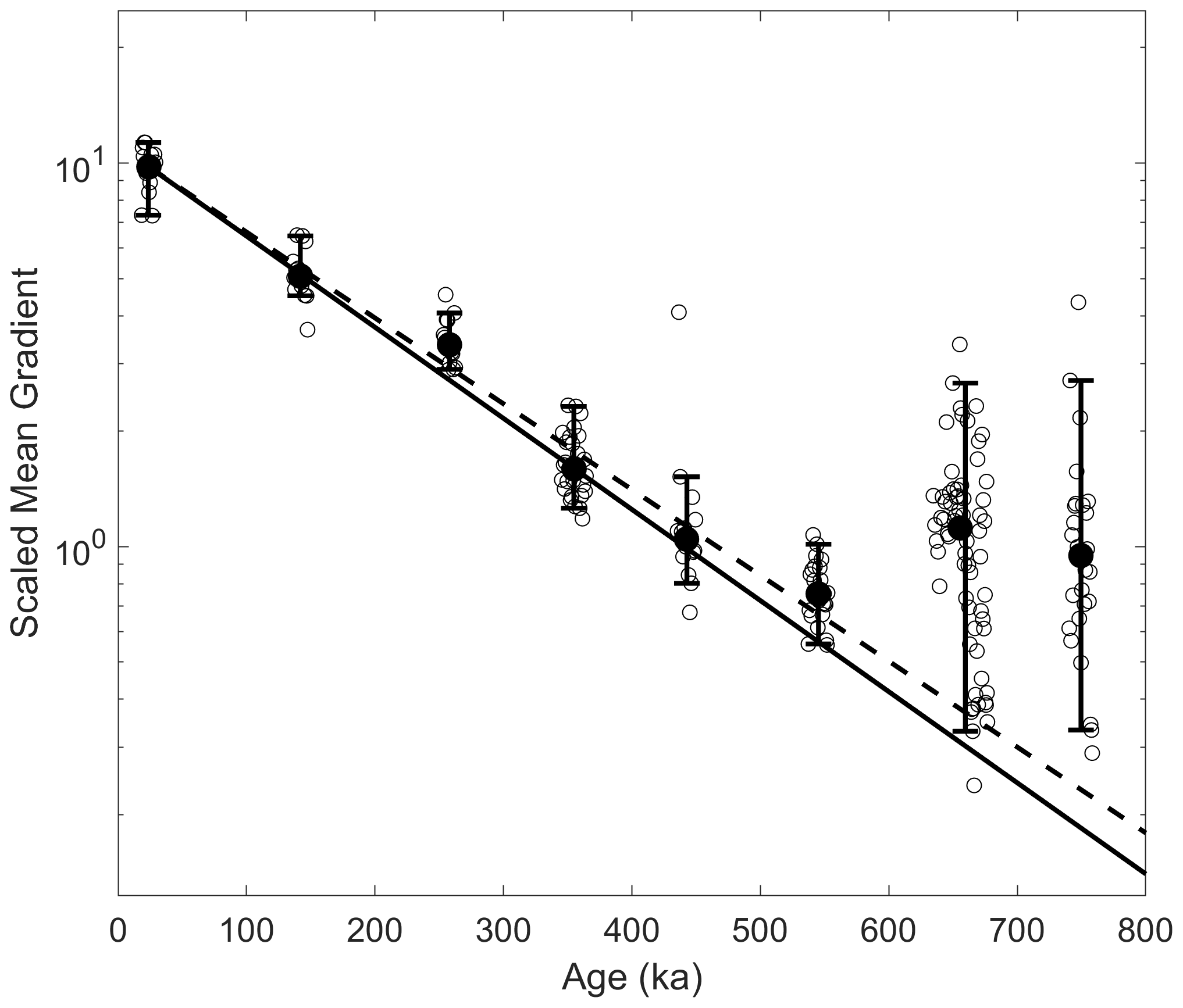
Figure 6The scaled mean gradients for eight glacial maximum periods are shown as black open circles. Analysis includes only glacial periods because the water isotope values for all glacial maximums are similar, while the older interglacials are not as comparable (Fig. 1). Medians of each glacial maximum are shown in solid black, and the range, excluding the largest and smallest in each time period, is shown with black whiskers. The most recent five glacial maximums are the same as in Fig. 4b. The solid black lines and dashed black lines are the same as in Fig. 4b; note the log y scale.
3.4 Deep ice older than 450 ka
We have thus far restricted the analysis to the most recent five glacial cycles because of the lack of interglacials with warm enough water isotope values to compare with similar characteristics at deposition. The glacial maximum water isotopes, however, are of similar values (Fig. 1), allowing three more periods to be considered. Figure 6 shows that the scaled mean gradients decrease with age through 545 ka; however, by 656 ka, the median scaled mean gradient has increased rather than continued to decrease. This occurs at about 3000 m depth. The variability also increases for the oldest two glacial maximum periods. The scaled mean gradients have not been corrected for artificial smoothing to ensure the increase is due to the measurements and not the correction.
The increase in scaled mean gradient for the final two glacial maximum periods is at first counterintuitive. An increase in effective diffusivity should reduce the scaled mean gradient. The increase in the scaled mean gradient likely occurs because sulfate has become mobile enough to form peaks unassociated with the sulfate concentrations at deposition. Traversi et al. (2009) noted that below about 2800 m depth there were sharp spikes in sulfate, with anomalous chemical compositions of low acidity and high magnesium. These peaks were not laterally homogenous. The scaled mean gradient at 545 ka shows a slight increase relative to the expectation, which may indicate some contribution of anomalous peaks; however, the increase is not substantial and suggests that if impurity interactions have begun then they remain limited.
4.1 Relation with temperature and grain size
The scaled mean gradient and the broadening of the largest volcanic peaks yield a similar result; the effective diffusivity of sulfate on timescales of hundreds of thousands of years is approximately m2 a−1 throughout most of the ice sheet until the ice warms near the bed. Our inferred value of the effective diffusivity is an order of magnitude smaller than that inferred from the Holocene data at EDC (B03). This result is consistent with the ability to find volcanic matches between EDC and Dome Fuji for the past 216 ka (Fujita et al., 2015), which would not be possible if the volcanic signals diffused at the previous estimate (Fig. 4). The smaller effective diffusivities we find could differ from the B03 Holocene values for two main reasons. First, processes may operate near the surface of the ice sheet, i.e., in the firn, that do not affect the record at greater depths. In this case, the higher Holocene effective diffusivity may be accurate but not appropriate to apply for the majority of the ice sheet depth. Second, the Holocene effective diffusivities may be inaccurate because of the challenges of noisy data and little time for diffusion to operate. We analyzed the Last Interglacial separately and found that the mean scaled gradients became larger with age, suggesting that inferences on short time periods may not be accurate.
Two different complications may affect our inference of the effective diffusivity. The first complication is artificial smoothing due to averaging over longer durations of time in samples of older ice. We estimated the impact of artificial smoothing (Sect. 2.4) and showed that the inferred effective diffusivity becomes smaller if it is included (Sect. 3.1); however, the artificial smoothing appears to be overestimated in the older ice. The second complication is rearrangement of impurities in deeper and warmer ice, which may include an increase in the lateral variability (Traversi et al., 2009). The rearrangement of impurities increases the scaled mean gradient and would decrease the inferred effective diffusivity. This process is thought to begin at about 2800 m depth (Traversi et al., 2009) and become more pronounced with depth as the ice warms and exceeds −10 ∘C; the bottom 60 m of ice are sufficiently altered so that no interpretable climate records are preserved (Tison et al., 2015). The rearrangement of impurities is unlikely to affect the more recent glacial cycle in the ice in the upper part of the ice sheet, even if alteration of the sulfate signal begins somewhat higher in the ice column than originally identified (e.g., Wolff et al., 2023). Both the artificial smoothing and the possible anomalous peaks are least likely to affect the estimate of effective diffusivity from the most recent glacial cycle (e.g., Holocene–LIG and LGM–PGM), and thus, we believe this period provides the most reliable estimate. The effective diffusivity inferred from the most recent glacial cycle fits the first five glacial cycles well (Fig. 4) and thus suggests that these two potential complications are not significant until older (deeper) ice is reached. Beyond the past five glacial cycles, post-depositional alteration of the chemical impurities (Fig. 6) becomes the dominant feature of the record, and the concept of an effective diffusivity is no longer useful.
The effective diffusivities of the interglacial and glacial maximum periods are within uncertainty for each other. This suggests that the total impurity concentration is not a significant control of the effective diffusivity, at least for concentrations typical of Antarctica. The higher impurity concentrations typical of Greenland or alpine cores may affect the effective diffusivity, and future estimates of the effective diffusivity from these locations would help decipher the role of impurities.
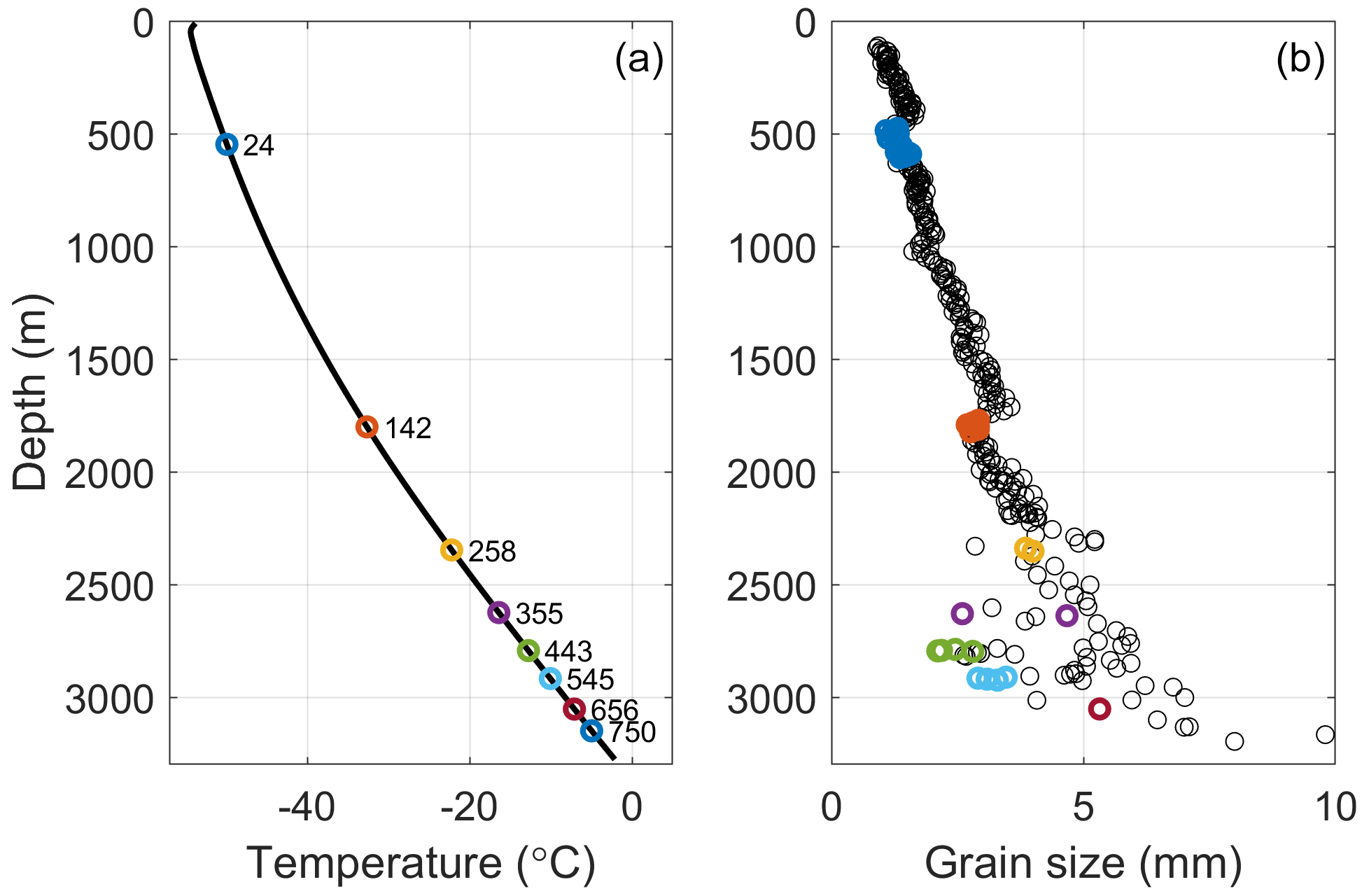
Figure 7(a) Temperature profile of EDC borehole (Buizert et al., 2021) with the glacial maximum periods plotted. (b) Grain size of EDC (Durand et al., 2006) with measurements within the glacial maximum periods plotted. Note that the oldest glacial maximum period (750 ka) has no grain size measurements within the time period.
There also is not a significant impact of temperature over the range of −55 ∘C at the surface to about −10 ∘C (3000 m depth). The borehole temperature profile at EDC (Buizert et al., 2021) is shown in Fig. 7a. The rate of diffusion does not appear to change with age and temperature, until the last two (possibly the last three) glacial maximums (Fig. 6), where multiple chemical species have become mobile enough to form anomalous sulfate peaks (Wolff et al., 2023). As suggested by Traversi et al. (2009), there appears to be a transition to a connected vein network which is not present at shallower depths and colder temperatures. While the transition is not a simple decrease in the variability in the sulfate record, it nonetheless suggests a zone where sulfate starts becoming mobile and the primary signal switches from a record of the atmospheric conditions at the time of deposition to a record of post-depositional alteration.
The modeling of diffusion of sulfate (e.g., Rempel et al., 2001, 2002; B03; Ng, 2021) has focused on sulfate in a vein network. However, the location of sulfate is not well established and will affect the ability of sulfate to diffuse. Our estimate of the effective diffusivity ( m2 a−1) is of the same order as the self-diffusion of ice ( m2 a−1 at −40 ∘C), suggesting that sulfate may reside in grains at colder temperatures. The self-diffusion of ice should be regarded as an upper limit (B03) for the diffusivity of sulfate and is still smaller than our estimate, which suggests some sulfate likely also resides in grain boundaries and veins, as well as in the crystal lattice.
The mechanisms for diffusion of sulfate have been linked to grain size and growth (Rempel et al., 2001; B03). Figure 7b shows that the grain size increases relatively little, particularly for the glacial maximum periods, likely due to impurities pinning grain boundaries (Durand et al., 2006). B03 developed two mechanisms for either a connected or disconnected vein network that were ultimately driven by grain growth. If net grain growth drives the solute movement, then the relatively constant rate of grain growth at EDC until ∼3000 m may explain why there is little noticeable impact of temperature. At depths below ∼3000 m and temperatures above −10 ∘C, the grain size starts to increase more rapidly. A temperature of −10 ∘C is unlikely to be a rigid threshold, as post-depositional processes are likely to start above this temperature (e.g., Traversi et al., 2009; Wolff et al., 2023) and are more likely to be a point at which the impurity interactions accelerate. The larger grains and corresponding larger veins likely allow greater impurity mobility. At EDC, this increase in mobility allows the sulfate to react with magnesium and other impurities, creating peaks unrelated to the concentration of sulfuric acid deposited at the surface.
4.2 Implications for ice older than 1 Ma
The locations of ice cores targeting 1.5 Ma ice (e.g., Fischer et al., 2013) will have similar site characteristics to Dome C and Dome Fuji. The European, Australian, and Japanese projects are located near the existing EDC and Dome Fuji cores (Lilien et al., 2021; Karlsson et al., 2018). The U.S. Center for Oldest Ice Exploration (COLDEX) is searching for a location in the interior of the East Antarctic plateau, while the Chinese effort is at Dome A, and the Russian project may be near Vostok. The low inferred effective diffusivity of sulfate suggests the volcanic climate records will be well preserved in these deep ice cores for at least the past few hundreds of thousands of years. However, the preservation of impurity signals for ice older than a few hundreds of thousands of years may depend on the basal temperature and whether the old ice has experienced considerable time at temperature above −10 ∘C, allowing large grains and likely connected vein networks to exist. Thus, ice core sites where the old ice remains cold, either due to a basal temperature well below the melting point or a basal ice layer that keeps the old ice farther from the bed, are likely to recover longer impurity records indicative of past climate variations.
The other type of location that has preserved ice older than 1 Ma is blue ice ablation areas (Higgins et al., 2015; Yan et al., 2019). The ice studied to date is not in stratigraphic order and thus records snapshots of past climate that average over an unknown interval of time. This ice has a complicated flow history, as revealed by the stratigraphic disturbances. The old ice has thus far been found between 100 and 200 m deep, where the ice temperature is close to the surface temperature of −30 ∘C for the Allan Hills. While the depths the ice reached on the path to its current location are not known, the maximum depth imaged upstream is about 1200 m (Kehrl et al., 2018). It is likely that the old ice in blue ice regions has never become warm enough (e.g., −10 ∘C) for the post-depositional processes found in the deep ice of EDC to become active.
4.3 Application to other ice cores
It is more difficult to compare the results from EDC to Antarctic ice cores with different site characteristics. We have investigated WDC (Fudge et al., 2016; McConnell, 2017), SPICEcore (Winski et al., 2019), EDML (Severi et al., 2012), and Talos Dome (Severi et al., 2015). Neither WDC nor South Pole Ice Core (SPICEcore) spans a full glacial cycle, and the sulfate data sets for EDML and Talos Dome do not extend past the last glacial period. This limits the ability to compare the evolution of the scaled mean gradient or volcanic widths for the same climate at deposition. We attempted to compare the scaled mean gradient and widths of volcanic events deposited in different climate states for EDC but could not find a reliable way to remove the influence of the climate at deposition. Thus, extending this analysis to these other ice cores was not possible.
Fudge et al. (2016) used the width of volcanic events at WDC to estimate the effective diffusivity but did not account for the different climate states at deposition. They found an effective diffusivity of m2 a−1 at −30 ∘C, using a temperature-dependent relationship; this effective diffusivity is half that of B03 but 4 times greater than inferred here. While we believe their methodology is not as robust as presented here, it is still worthwhile to consider why the two estimates might differ. The depth–age relationships are very different. The accumulation rate and vertical thinning is much greater at WDC; for instance, the LGM ice at EDC is 87 % of its original thickness, while at WDC it is 31 % of the original thickness. The higher rate of vertical thinning at WDC may lead to a higher effective diffusivity, particularly if the effective diffusivity is linked to grain growth and nucleation processes (B03). The grain size at WDC (Fitzpatrick et al., 2014) is smaller than EDC for all depths greater than 500 m, so the net grain growth would not be the cause of a higher effective diffusivity at WDC.
The WDC volcanic widths were fit with an effective diffusivity with an assumed temperature dependence. We note that the temperature dependence is not well constrained by the data, given the uncertainties in the volcanic widths. Thus, WDC neither supports nor refutes the lack of temperature dependence of the effective diffusivity at temperature below ∘C. WDC is in agreement that above −10 ∘C the effective diffusivity seems to change. Fudge et al. (2016) did not identify peaks at ages older than 52 ka, and the synchronization of WDC with other East Antarctic cores (Buizert et al., 2018) stopped at 58 ka, despite a bottom age of 67 ka at WDC. These depths and ages correspond approximately to a −10 ∘C temperature in the ice sheet (Cuffey et al., 2016). No anomalous sulfate peaks were observed at WDC, which may be due to the much shorter duration that the ice has spent at the warm temperature (i.e., tens of thousands of years at WDC compared to hundreds of thousands of years at EDC). Future work is needed to better constrain the effective diffusivity of sulfate in ice cores with higher accumulation rates than the interior of the East Antarctic plateau.
4.4 Implications for existing timescales and estimates of volcanic forcing
The effective diffusivity of m2 a−1 is low enough that volcanic events in the Holocene are not significantly impacted by diffusion. After 10 ka, the amplitude is reduced by only 6 %. Since detection algorithms (Cole-Dai et al., 2021; Sigl et al., 2015) take the background level into account and calculate the sulfate flux onto the ice sheet over multiple years, there is likely to be little change in the flux estimates. The flux estimates will not be significantly impacted until the peaks have diffused enough to blend into and increase the background levels. Reconstructions of atmospheric sulfate from bipolar ice core records now extend through the Holocene (Sigl et al., 2022; Lin et al., 2022) and may be extended farther as volcanic matches in the glacial period are identified (Svensson et al., 2020). The impact of diffusion on the volcanic flux will be more important to consider for older ages.
Our results also show that diffusion is unlikely to substantially impact the synchronization of Antarctic timescale through the last glacial period (e.g., Ruth et al., 2007; Severi et al., 2012; Buizert et al., 2018). After 50 ka, the amplitude has been reduced by only 30 %. However, by 100 ka the reduction has increased to 55 %, such that less than half the original amplitude remains. There is no precise point at which volcanic events cannot be distinguished because it depends on the original amplitude and the background variability, neither of which are constant. It is a bit surprising that the synchronization of EDC and Dome Fuji (Fujita et al., 2015) matched approximately twice as many events in the LIG (∼10 per 1 ka) as in the Holocene (∼5 per 1 ka), despite diffusion acting to reduce the peak amplitudes by more than half; the LIG may have had greater volcanic activity, allowing more matches. Synchronizations extending beyond the current 210 ka limit may be possible, particularly with better sampling resolution to limit artificial smoothing in the records.
4.5 Limitations and future work
In this work, we have focused on obtaining a single estimate and uncertainty for the effective diffusivity for sulfuric acid. The inferred effective diffusivities range by about a factor of 5 (Table 2). Many of these differences are likely driven by uncertainty in the data and methods; however, the effective diffusivity may also vary for different conditions in the ice sheet. Our inferences are based on average properties or groups of volcanic events and may be integrating the impacts of multiple diffusive processes. While we did not find an obvious temperature dependence, there is likely an interplay between higher sulfuric acid concentrations and warmer temperatures allowing more premelting (Dash et al., 2006), particularly if the sulfuric acid resides primarily at grain boundaries. More liquid at grain boundaries should change the effective diffusivity locally, although related changes to the grain growth rate may be necessary for a noticeable impact (e.g., Rempel et al., 2001; B03). The sulfuric acid concentration thus may create a nonlinearity where the effective diffusivity depends on the concentration. The lack of knowledge of the portion of sulfuric acid located at grain boundaries compared to within grain lattices is a particular limitation. Where the sulfuric acid is located may depend on the conditions at deposition or the post-depositional processes involved in grain growth and nucleation, such that different diffusive mechanisms are more important at different locations within the ice, potentially changing the effective diffusivity through time.
The challenges in observing where sulfuric acid resides (Mulvaney et al., 1988; Fukuzawa et al., 1998) limits the ability to accurately model diffusive processes. Isolation of different diffusive mechanisms may be possible with lab-grown ice doped with sulfuric acid (e.g., Hammonds and Baker, 2018) if the ice is grown such that the acid is located either within the grains or at the grain boundaries and then deformed and changes in the location identified. Estimates of effective diffusivity can also be extended to other impurities, as B03 originally did for chloride and sodium. The differences in effective diffusivity among impurities may also help to distinguish processes that affect all impurities from those that are specific to an individual impurity. With multiple international projects focused on interpreting ice of 1 Ma and older, which has been strained to a small fraction of its initial thickness, more work in understanding the preservation and post-depositional alteration of impurities, as well as gases and water isotopes, will be necessary for confident interpretation of past climatic variations.
The long temporal record at EDC allows the effective diffusivity of sulfate to be estimated using multiple glacial cycles. By comparing the characteristics of the sulfate record exclusively in either interglacial or glacial maximum periods, the effect of differences in the climate at deposition can be minimized. We found an effective diffusivity of m2 a−1. That value is an order of magnitude lower than the value that was previously inferred at EDC using only Holocene data (B03). The ECM data from Dome Fuji for the past glacial cycle agrees well with our estimate from EDC. The uncertainty is difficult to quantify, but we suggest a value of m2 a−1. Our estimate of the effective diffusivity is most applicable for timescales of hundreds of thousands of years and for temperatures colder than −10 ∘C. In the deep ice warmer than −10 ∘C, the variability in the sulfate record increases due to anomalous sulfate peaks (Traversi et al., 2009) caused by impurity movement and marks the end of the sulfate record being indicative of the climate history. In the upper ∼90 % of the ice sheet, the low effective diffusivity suggests that sulfuric acid is not readily diffusing in liquid-like veins; however, in the deep ice a connected vein network appears to allow the climate variations to be replaced by peaks generated after deposition. The low effective diffusivity for the cold ice in the upper portion of the ice sheet suggests that sulfuric acid and other impurity records might be preserved in deep, old ice if the ice temperature remains well below the pressure melting point.
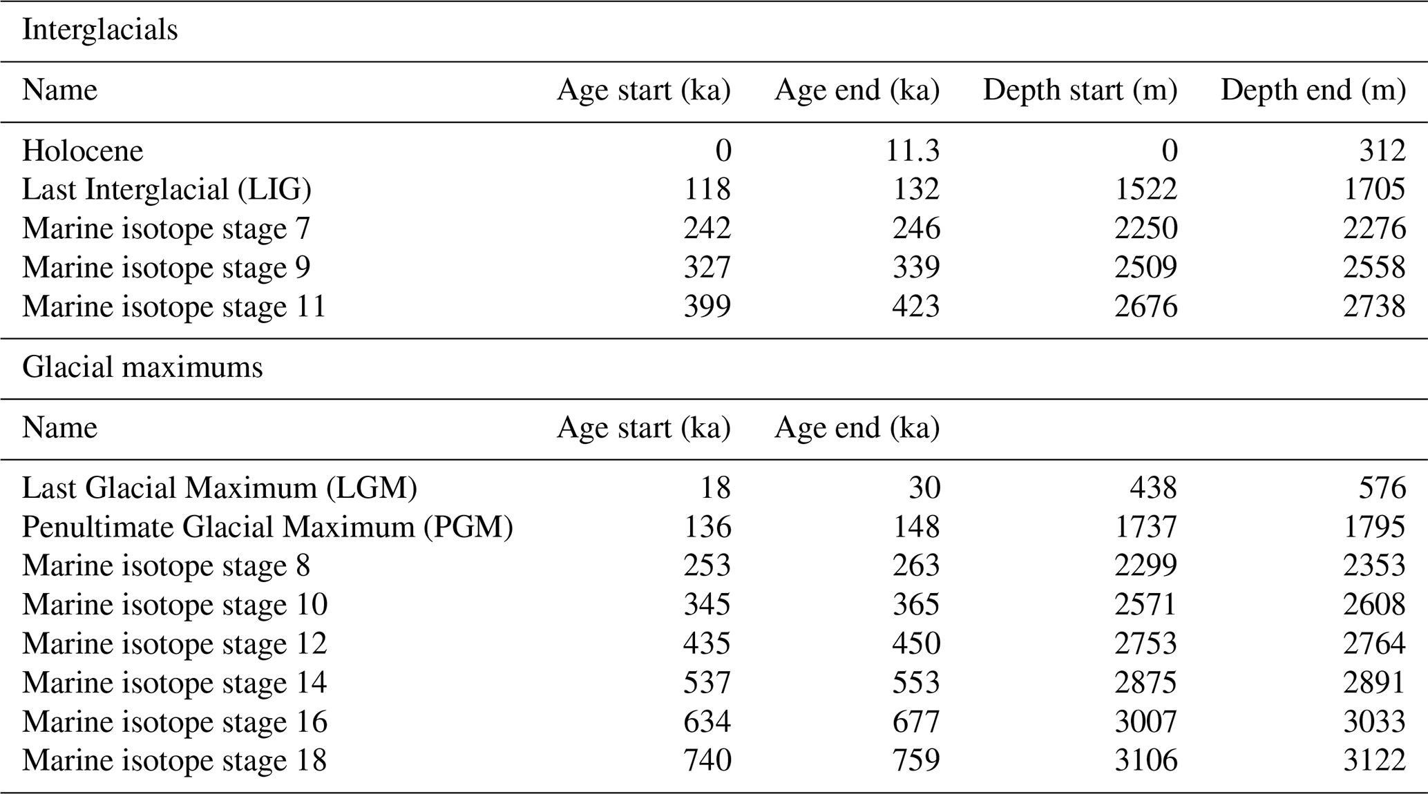
We used the age and depth ranges in Table A1 for the interglacial and glacial maximum periods.
Table A1Age and depth ranges of interglacial and glacial maximum periods.
All code is available upon request to tjfudge@uw.edu. The calculation of the mean scaled gradient is well described in Barnes et al. (2003) and was replicated here.
The EDC sulfate data are available at https://doi.org/10.15784/601759 (Fudge and Severi, 2023) and https://doi.org/10.25921/kgv8-cn35 (Severi et al., 2020).
TJF designed the study and wrote the article. RS, BHH, and TJF performed scaled mean gradient analysis. LV and TJF performed the volcanic width analysis. MS provided the sulfate data. EDW inspired and guided the project. All authors contributed to the paper.
The contact author has declared that none of the authors has any competing interests.
Publisher's note: Copernicus Publications remains neutral with regard to jurisdictional claims made in the text, published maps, institutional affiliations, or any other geographical representation in this paper. While Copernicus Publications makes every effort to include appropriate place names, the final responsibility lies with the authors.
This article is part of the special issue “Oldest Ice: finding and interpreting climate proxies in ice older than 700 000 years (TC/CP/ESSD inter-journal SI)”. It is not associated with a conference.
We thank NSF and the Washington NASA Space Grant Summer Undergraduate Research Program for supporting Raphael Sauvage and Linh Vu. We also thank Rachael Rhodes and Eric Wolff for helpful discussions at the IPICS2022 meeting. We thank two anonymous reviewers for improving the paper.
This research has been supported by the Directorate for Geosciences, Office of Polar Programs (grant no. 1851022).
This paper was edited by Carlo Barbante and reviewed by two anonymous referees.
Aydin, M., Fudge, T. J., Verhulst, K. R., Nicewonger, M. R., Waddington, E. D., and Saltzman, E. S.: Carbonyl sulfide hydrolysis in Antarctic ice cores and an atmospheric history for the last 8000 years, J. Geophys. Res.-Atmos., 119, 8500–8514, https://doi.org/10.1002/2014JD021618, 2014.
Barnes, P. R. F. and Wolff, E. W.: Distribution of soluble impurities in cold glacial ice, J. Glaciol., 50, 311–324, 2004.
Barnes, P. R. F., Wolff, E. W., Mader, H. M., Udisti, R., Castellano, E., and Rothlisberger, R.: Evolution of chemical peak shapes in the Dome C, Antarctica, ice core, J. Geophys. Res.-Atmos., 108, 4126, 2003.
Bazin, L., Landais, A., Lemieux-Dudon, B., Toyé Mahamadou Kele, H., Veres, D., Parrenin, F., Martinerie, P., Ritz, C., Capron, E., Lipenkov, V., Loutre, M.-F., Raynaud, D., Vinther, B., Svensson, A., Rasmussen, S. O., Severi, M., Blunier, T., Leuenberger, M., Fischer, H., Masson-Delmotte, V., Chappellaz, J., and Wolff, E.: An optimized multi-proxy, multi-site Antarctic ice and gas orbital chronology (AICC2012): 120–800 ka, Clim. Past, 9, 1715–1731, https://doi.org/10.5194/cp-9-1715-2013, 2013.
Bereiter, B., Fischer, H., Schwander, J., and Stocker, T. F.: Diffusive equilibration of N2, O2 and CO2 mixing ratios in a 1.5-million-years-old ice core, The Cryosphere, 8, 245–256, https://doi.org/10.5194/tc-8-245-2014, 2014.
Buizert, C., Sigl, M., Severi, M., Markle, B. R., Wettstein, J. J., McConnell, J. R., Pedro, J. B., Sodemann, H., Goto-Azuma, K., Kawamura, K., Fujita, S., Motoyama, H., Hirabayashi, M., Uemura, R., Stenni, B., Parrenin, F., He, F., Fudge, T. J., and Steig, E. J.: Abrupt ice-age shifts in southern westerly winds and Antarctic climate forced from the north, Nature, 563, 681–685, 2018.
Buizert, C., Fudge, T. J., Roberts, W. H. G., Steig, E. J., Sherriff-Tadano, S., Ritz, C., Lefebvre, E., Edwards, J., Kawamura, K., Oyabu, I., Motoyama, H., Kahle, E. C., Jones, T. R., Abe-Ouchi, A., Obase, T., Martin, C., Corr, H., Severinghaus, J. P., Beaudette, R., Epifanio, J. A., Brook, E. J., Martin, K., Chappellaz, J., Aoki, S., Nakazawa, T., Sowers, T. A., Alley, R. B., Ahn, J., Sigl, M., Severi, M., Dunbar, N. W., Svensson, A., Fegyveresi, J. M., He, C. F., Liu, Z. Y., Zhu, J., Otto-Bliesner, B. L., Lipenkov, V. Y., Kageyama, M., and Schwander, J.: Antarctic surface temperature and elevation during the Last Glacial Maximum, Science, 372, 1097–1101, 2021.
Cole-Dai, J., Ferris, D. G., Kennedy, J. A., Sigl, M., McConnell, J. R., Fudge, T. J., Geng, L., Maselli, O. J., Taylor, K. C., and Souney, J. M.: Comprehensive Record of Volcanic Eruptions in the Holocene (11,000 years) From the WAIS Divide, Antarctica Ice Core, J. Geophys. Res.-Atmos., 126, e2020JD032855, https://doi.org/10.1029/2020JD032855, 2021.
Cuffey, K. M. and Steig, E. J.: Isotopic diffusion in polar firn: implications for interpretation of seasonal climate parameters in ice-core records, with emphasis on central Greenland, J. Glaciol., 44, 273–284, 1998.
Cuffey, K. M., Clow, G. D., Steig, E. J., Buizert, C., Fudge, T. J., Koutnik, M., Waddington, E. D., Alley, R. B., and Severinghaus, J. P.: Deglacial temperature history of West Antarctica, P. Natl. Acad. Sci. USA, 113, 14249–14254, https://doi.org/10.1073/pnas.1609132113, 2016.
Dash, J. G., Rempel, A. W., and Wettlaufer, J. S.: The physics of premelted ice and its geophysical consequences, Rev. Modern Phys., 78, 695–741, 2006.
Dibb, J. E., Talbot, R. W., Munger, J. W., Jacob, D. J., and Fan, S. M.: Air-snow exchange of HNO3 and NOy at Summit, Greenland, J. Geophys. Res.-Atmos., 103, 3475–3486, 1998.
Durand, G., Weiss, J., Lipenkov, V., Barnola, J. M., Krinner, G., Parrenin, F., Delmonte, B., Ritz, C., Duval, P., Rothlisberger, R., and Bigler, M.: Effect of impurities on grain growth in cold ice sheets, J. Geophys. Res.-Earth Surf., 111, F01015, https://doi.org/10.1029/2005JF000320, 2006.
EPICA: Eight glacial cycles from an Antarctic ice core, Nature, 429, 623–628, 2004.
Fischer, H., Severinghaus, J., Brook, E., Wolff, E., Albert, M., Alemany, O., Arthern, R., Bentley, C., Blankenship, D., Chappellaz, J., Creyts, T., Dahl-Jensen, D., Dinn, M., Frezzotti, M., Fujita, S., Gallee, H., Hindmarsh, R., Hudspeth, D., Jugie, G., Kawamura, K., Lipenkov, V., Miller, H., Mulvaney, R., Parrenin, F., Pattyn, F., Ritz, C., Schwander, J., Steinhage, D., van Ommen, T., and Wilhelms, F.: Where to find 1.5 million yr old ice for the IPICS “Oldest-Ice” ice core, Clim. Past, 9, 2489–2505, https://doi.org/10.5194/cp-9-2489-2013, 2013.
Fitzpatrick, J. J., Voigt, D. E., Fegyveresi, J. M., Stevens, N. T., Spencer, M. K., Cole-Dai, J., Alley, R. B., Jardine, G. E., Cravens, E. D., Wilen, L. A., Fudge, T. J., and Mcconnell, J. R.: Physical properties of the WAIS Divide ice core, J. Glaciol., 60, 1181–1198, https://doi.org/10.3189/2014JoG14J100, 2014.
Fudge, T. J. and Severi, M.: EPICA Dome C Sulfate Data 7–3190 m, U.S. Antarctic Program (USAP) Data Center [data set], https://doi.org/10.15784/601759, 2023.
Fudge, T. J., Taylor, K. C., Waddington, E. D., Fitzpatrick, J. J., and Conway, H.: Electrical stratigraphy of the WAIS Divide ice core: Identification of centimeter-scale irregular layering, J. Geophys. Res.-Earth Surf., 121, 1218–1229, 2016.
Fujita, S., Azuma, N., Motoyama, H., Kameda, T., Narita, H., Fujii, Y., and Watanabe, O.: Electrical measurements on the 2503 m Dome F Antarctic ice core, Ann. Glaciol., 35, 313–320, https://doi.org/10.3189/172756402781816951, 2002.
Fujita, S., Parrenin, F., Severi, M., Motoyama, H., and Wolff, E. W.: Volcanic synchronization of Dome Fuji and Dome C Antarctic deep ice cores over the past 216 kyr, Clim. Past, 11, 1395–1416, https://doi.org/10.5194/cp-11-1395-2015, 2015.
Fukazawa, H., Sugiyama, K., Mae, S. J., Narita, H., and Hondoh, T.: Acid ions at triple junction of Antarctic ice observed by Raman scattering, Geophys. Res. Lett., 25, 2845–2848, 1998.
Gkinis, V., Simonsen, S. B., Buchardt, S. L., White, J. W. C., and Vinther, B. M.: Water isotope diffusion rates from the NorthGRIP ice core for the last 16,000 years – Glaciological and paleoclimatic implications, Earth Planet. Sc. Lett., 405, 132–141, 2014.
Hammonds, K. and Baker, I.: The effects of H2SO4 on the mechanical behavior and microstructural evolution of polycrystalline ice, J. Geophys. Res.-Earth Surf., 123, 535–556, 2018.
Higgins, J. A., Kurbatov, A. V., Spaulding, N. E., Brook, E., Introne, D. S., Chimiak, L. M., Yan, Y. Z., Mayewski, P. A., and Bender, M. L.: Atmospheric composition 1 million years ago from blue ice in the Allan Hills, Antarctica, P. Natl. Acad. Sci. USA, 112, 6887–6891, 2015.
Johnsen, S. J., Clausen, H. B., Cuffey, K. M., Hoffmann, G., Schwander, J., and Creyts, T.: Diffusion of stable isotopes in polar firn and ice: The isotope effect in firn diffusion, in: Physics of ice core records, edited by: Hondoh, T., 121–140, Hokkaido University Press, Sapporo, 2000.
Kahle, E. C., Steig, E. J., Jones, T. R., Fudge, T. J., Koutnik, M. R., Morris, V. A., Vaughn, B. H., Schauer, A. J., Stevens, C. M., Conway, H., Waddington, E. D., Buizert, C., Epifanio, J., and White, J. W. C.: Reconstruction of Temperature, Accumulation Rate, and Layer Thinning From an Ice Core at South Pole, Using a Statistical Inverse Method, J. Geophys. Res.-Atmos., 126, e2020JD033300, https://doi.org/10.1029/2020JD033300, 2021.
Karlsson, N. B., Binder, T., Eagles, G., Helm, V., Pattyn, F., Van Liefferinge, B., and Eisen, O.: Glaciological characteristics in the Dome Fuji region and new assessment for “Oldest Ice”, The Cryosphere, 12, 2413–2424, https://doi.org/10.5194/tc-12-2413-2018, 2018.
Kehrl, L., Conway, H., Holschuh, N., Campbell, S., Kurbatov, A. V., and Spaulding, N. E.: Evaluating the Duration and Continuity of Potential Climate Records From the Allan Hills Blue Ice Area, East Antarctica, Geophys. Res. Lett., 45, 4096–4104, 2018.
Legrand, M.: Sulphur-Derived Species in Polar Ice: A Review, in: Ice Core Studies of Global Biogeochemical Cycles, edited by: Delmas, R. J., NATO ASI Series, Springer, Berlin, Heidelberg, 30, https://doi.org/10.1007/978-3-642-51172-1_5, 1995.
Lilien, D. A., Steinhage, D., Taylor, D., Parrenin, F., Ritz, C., Mulvaney, R., Martín, C., Yan, J.-B., O'Neill, C., Frezzotti, M., Miller, H., Gogineni, P., Dahl-Jensen, D., and Eisen, O.: Brief communication: New radar constraints support presence of ice older than 1.5 Myr at Little Dome C, The Cryosphere, 15, 1881–1888, https://doi.org/10.5194/tc-15-1881-2021, 2021.
Lin, J., Svensson, A., Hvidberg, C. S., Lohmann, J., Kristiansen, S., Dahl-Jensen, D., Steffensen, J. P., Rasmussen, S. O., Cook, E., Kjær, H. A., Vinther, B. M., Fischer, H., Stocker, T., Sigl, M., Bigler, M., Severi, M., Traversi, R., and Mulvaney, R.: Magnitude, frequency and climate forcing of global volcanism during the last glacial period as seen in Greenland and Antarctic ice cores (60–9 ka), Clim. Past, 18, 485–506, https://doi.org/10.5194/cp-18-485-2022, 2022.
McConnell, J.: WAIS Divide Ice-Core Aerosol Records from 1300 to 3404 m, U.S. Antarctic Program (USAP) Data Center [data set], https://doi.org/10.15784/601008, 2017.
Mulvaney, R., Wolff, E. W., and Oates, K.: Sulfuric-acid at grain-boundaries in Antarctic ice, Nature, 331, 247–249, 1988.
Nardin, R., Amore, A., Becagli, S., Caiazzo, L., Frezzotti, M., Severi, M., Stenni, B., and Traversi, R.: Volcanic Fluxes Over the Last Millennium as Recorded in the Gv7 Ice Core (Northern Victoria Land, Antarctica), Geosciences, 10, 38, https://doi.org/10.3390/geosciences10010038, 2020.
NEEM: Eemian interglacial reconstructed from a Greenland folded ice core, Nature, 493, 489–494, 2013.
Ng, F. S. L.: Pervasive diffusion of climate signals recorded in ice-vein ionic impurities, The Cryosphere, 15, 1787–1810, https://doi.org/10.5194/tc-15-1787-2021, 2021.
Ohno, H., Igarashi, M., and Hondoh, T.: Salt inclusions in polar ice core: Location and chemical form of water-soluble impurities, Earth Planet. Sc. Lett., 232, 171–178, 2005.
Osman, M., Das, S. B., Marchal, O., and Evans, M. J.: Methanesulfonic acid (MSA) migration in polar ice: data synthesis and theory, The Cryosphere, 11, 2439–2462, https://doi.org/10.5194/tc-11-2439-2017, 2017.
Pasteur, E. C. and Mulvaney, R.: Migration of methane sulphonate in Antarctic firn and ice, J. Geophys. Res.-Atmos., 105, 11525–11534, 2000.
Rempel, A. W., Waddington, E. D., Wettlaufer, J. S., and Worster, M. G.: Possible displacement of the climate signal in ancient ice by premelting and anomalous diffusion, Nature, 411, 568–571, 2001.
Rempel, A. W., Wettlaufer, J. S., and Waddington, E. D.: Anomalous diffusion of multiple impurity species: Predicted implications for the ice core climate records, J. Geophys. Res.-Sol. Ea., 107, 2330, https://doi.org/10.1029/2002JB001857, 2002.
Ruth, U., Barnola, J.-M., Beer, J., Bigler, M., Blunier, T., Castellano, E., Fischer, H., Fundel, F., Huybrechts, P., Kaufmann, P., Kipfstuhl, S., Lambrecht, A., Morganti, A., Oerter, H., Parrenin, F., Rybak, O., Severi, M., Udisti, R., Wilhelms, F., and Wolff, E.: “EDML1”: a chronology for the EPICA deep ice core from Dronning Maud Land, Antarctica, over the last 150 000 years, Clim. Past, 3, 475–484, https://doi.org/10.5194/cp-3-475-2007, 2007.
Severi, M., Becagli, S., Castellano, E., Morganti, A., Traversi, R., Udisti, R., Ruth, U., Fischer, H., Huybrechts, P., Wolff, E., Parrenin, F., Kaufmann, P., Lambert, F., and Steffensen, J. P.: Synchronisation of the EDML and EDC ice cores for the last 52 kyr by volcanic signature matching, Clim. Past, 3, 367–374, https://doi.org/10.5194/cp-3-367-2007, 2007.
Severi, M., Udisti, R., Becagli, S., Stenni, B., and Traversi, R.: Volcanic synchronisation of the EPICA-DC and TALDICE ice cores for the last 42 kyr BP, Clim. Past, 8, 509–517, https://doi.org/10.5194/cp-8-509-2012, 2012.
Severi, M., Becagli, S., Traversi, R., and Udisti, R.: Recovering Paleo-Records from Antarctic Ice-Cores by Coupling a Continuous Melting Device and Fast Ion Chromatography, Anal. Chem., 87, 11441–11447, https://doi.org/10.1021/acs.analchem.5b02961, 2015.
Severi, M., Udisti, R., Castellano, E., and Wolff, E. W.: NOAA/WDS Paleoclimatology – EPICA Dome C 203 000 Year High-Resolution FIC Sulfate Data, NOAA National Centers for Environmental Information [data set], https://doi.org/10.25921/kgv8-cn35, 2020.
Sigl, M., McConnell, J. R., Layman, L., Maselli, O., McGwire, K., Pasteris, D., Dahl-Jensen, D., Steffensen, J. P., Vinther, B., Edwards, R., Mulvaney, R., and Kipfstuhl, S.: A new bipolar ice core record of volcanism from WAIS Divide and NEEM and implications for climate forcing of the last 2000 years, J. Geophys. Res.-Atmos., 118, 1151–1169, 2013.
Sigl, M., Winstrup, M., McConnell, J. R., Welten, K. C., Plunkett, G., Ludlow, F., Buntgen, U., Caffee, M., Chellman, N., Dahl-Jensen, D., Fischer, H., Kipfstuhl, S., Kostick, C., Maselli, O. J., Mekhaldi, F., Mulvaney, R., Muscheler, R., Pasteris, D. R., Pilcher, J. R., Salzer, M., Schupbach, S., Steffensen, J. P., Vinther, B. M., and Woodruff, T. E.: Timing and climate forcing of volcanic eruptions for the past 2,500 years, Nature, 523, 543–546, 2015.
Sigl, M., Toohey, M., McConnell, J. R., Cole-Dai, J., and Severi, M.: Volcanic stratospheric sulfur injections and aerosol optical depth during the Holocene (past 11 500 years) from a bipolar ice-core array, Earth Syst. Sci. Data, 14, 3167–3196, https://doi.org/10.5194/essd-14-3167-2022, 2022.
Svensson, A., Bigler, M., Blunier, T., Clausen, H. B., Dahl-Jensen, D., Fischer, H., Fujita, S., Goto-Azuma, K., Johnsen, S. J., Kawamura, K., Kipfstuhl, S., Kohno, M., Parrenin, F., Popp, T., Rasmussen, S. O., Schwander, J., Seierstad, I., Severi, M., Steffensen, J. P., Udisti, R., Uemura, R., Vallelonga, P., Vinther, B. M., Wegner, A., Wilhelms, F., and Winstrup, M.: Direct linking of Greenland and Antarctic ice cores at the Toba eruption (74 ka BP), Clim. Past, 9, 749–766, https://doi.org/10.5194/cp-9-749-2013, 2013.
Svensson, A., Dahl-Jensen, D., Steffensen, J. P., Blunier, T., Rasmussen, S. O., Vinther, B. M., Vallelonga, P., Capron, E., Gkinis, V., Cook, E., Kjær, H. A., Muscheler, R., Kipfstuhl, S., Wilhelms, F., Stocker, T. F., Fischer, H., Adolphi, F., Erhardt, T., Sigl, M., Landais, A., Parrenin, F., Buizert, C., McConnell, J. R., Severi, M., Mulvaney, R., and Bigler, M.: Bipolar volcanic synchronization of abrupt climate change in Greenland and Antarctic ice cores during the last glacial period, Clim. Past, 16, 1565–1580, https://doi.org/10.5194/cp-16-1565-2020, 2020.
Tison, J.-L., de Angelis, M., Littot, G., Wolff, E., Fischer, H., Hansson, M., Bigler, M., Udisti, R., Wegner, A., Jouzel, J., Stenni, B., Johnsen, S., Masson-Delmotte, V., Landais, A., Lipenkov, V., Loulergue, L., Barnola, J.-M., Petit, J.-R., Delmonte, B., Dreyfus, G., Dahl-Jensen, D., Durand, G., Bereiter, B., Schilt, A., Spahni, R., Pol, K., Lorrain, R., Souchez, R., and Samyn, D.: Retrieving the paleoclimatic signal from the deeper part of the EPICA Dome C ice core, The Cryosphere, 9, 1633–1648, https://doi.org/10.5194/tc-9-1633-2015, 2015.
Traufetter, F., Oerter, H., Fischer, H., Weller, R., and Miller, H.: Spatio-temporal variability in volcanic sulphate deposition over the past 2 kyr in snow pits and firn cores from Amundsenisen, Antarctica, J. Glaciol., 50, 137–146, 2004.
Traversi, R., Becagli, S., Castellano, E., Marino, F., Rugi, F., Severi, M., de Angelis, M., Fischer, H., Hansson, M., Stauffer, B., Steffensen, J. P., Bigler, M., and Udisti, R.: Sulfate Spikes in the Deep Layers of EPICA-Dome C Ice Core: Evidence of Glaciological Artifacts, Environ. Sci. Technol., 43, 8737–8743, 2009.
Veres, D., Bazin, L., Landais, A., Toyé Mahamadou Kele, H., Lemieux-Dudon, B., Parrenin, F., Martinerie, P., Blayo, E., Blunier, T., Capron, E., Chappellaz, J., Rasmussen, S. O., Severi, M., Svensson, A., Vinther, B., and Wolff, E. W.: The Antarctic ice core chronology (AICC2012): an optimized multi-parameter and multi-site dating approach for the last 120 thousand years, Clim. Past, 9, 1733–1748, https://doi.org/10.5194/cp-9-1733-2013, 2013.
WDPM (WAIS Divide Project Members): Onset of deglacial warming in West Antarctica driven by local orbital forcing, Nature, 500, 440–444, 2013.
Winski, D. A., Fudge, T. J., Ferris, D. G., Osterberg, E. C., Fegyveresi, J. M., Cole-Dai, J., Thundercloud, Z., Cox, T. S., Kreutz, K. J., Ortman, N., Buizert, C., Epifanio, J., Brook, E. J., Beaudette, R., Severinghaus, J., Sowers, T., Steig, E. J., Kahle, E. C., Jones, T. R., Morris, V., Aydin, M., Nicewonger, M. R., Casey, K. A., Alley, R. B., Waddington, E. D., Iverson, N. A., Dunbar, N. W., Bay, R. C., Souney, J. M., Sigl, M., and McConnell, J. R.: The SP19 chronology for the South Pole Ice Core – Part 1: volcanic matching and annual layer counting, Clim. Past, 15, 1793–1808, https://doi.org/10.5194/cp-15-1793-2019, 2019.
Wolff, E. W., Burke, A., Crick, L., Doyle, E. A., Innes, H. M., Mahony, S. H., Rae, J. W. B., Severi, M., and Sparks, R. S. J.: Frequency of large volcanic eruptions over the past 200 000 years, Clim. Past, 19, 23–33, https://doi.org/10.5194/cp-19-23-2023, 2023.
Yan, Y. Z., Bender, M. L., Brook, E. J., Clifford, H. M., Kemeny, P. C., Kurbatov, A. V., Mackay, S., Mayewski, P. A., Ng, J., Severinghaus, J. P., and Higgins, J. A.: Two-million-year-old snapshots of atmospheric gases from Antarctic ice, Nature, 574, 663–666, 2019.
Zielinski, G. A., Mayewski, P. A., Meeker, L. D., Gronvold, K., Germani, M. S., Whitlow, S., Twickler, M. S., and Taylor, K.: Volcanic aerosol records and tephrochronology of the Summit, Greenland, ice cores, J. Geophys. Res.-Oceans,, 102, 26625–26640, 1997.