Could old tide gauges help estimate past atmospheric variability?

The surge residual is the non-tidal component of coastal sea level. It responds to the atmospheric circulation, including the direct effect of atmospheric pressure on the sea surface. Tide gauges have been used to measure the sea level in coastal cities for centuries, with many records dating back to the 19th century or even earlier to times when direct pressure observations were scarce. Therefore, these old tide gauge records may be used as indirect observations of sub-seasonal atmospheric variability that are complementary to other sensors such as barometers. To investigate this claim, the present work relies on the tide gauge record of Brest, western France, and on the members of NOAA's 20th Century Reanalysis (20CRv3), which only assimilates surface pressure observations and uses a numerical weather prediction model. Using simple statistical relationships between surge residuals and local atmospheric pressure, we show that the tide gauge record can help to reveal part of the 19th century atmospheric variability that was uncaught by the pressure-observations-based reanalysis, advocating for the use of early tide gauge records to study past storms. In particular, weighting the 80 reanalysis members based on tide gauge observations indicates that a large number of members seem unlikely, which induces corrections of several tens of hectopascals in the Bay of Biscay. Comparisons with independent pressure observations shed light on the strengths and limitations of the methodology, particularly for the case of wind-driven surge residuals. This calls for the future use of a mixed methodology between data-driven tools and physics-based modeling. Our methodology could be applied to use other types of independent observations (not just tide gauges) as a means of weighting reanalysis ensemble members.

1 Introduction

Understanding the atmospheric system requires an understanding of all scales of variation from daily to centennial. This cannot be done unless long observation records allow the disentanglement of these scales. The 20th Century Reanalysis Project, hereafter “20CR” (Compo et al., 2011), which is now in its third version, hereafter “20CRv3” (Slivinski et al., 2019), is the only atmospheric reanalysis that runs through the 19th century. It relies on the International Surface Pressure Databank (Compo et al., 2019), the largest historical global collection of surface pressure observations, and the NCEP Global Forecast System (GFS) coupled atmosphere–land model.

Because it is the longest atmospheric reanalysis available, 20CR is used to study possible long-term trends in atmospheric dynamics (Rodrigues et al., 2018) or for extreme events (Alvarez-Castro et al., 2018). However, although the 20th century part of 20CR has been compared with other reanalyses (Wohland et al., 2019) and observations (Krueger et al., 2013), comparisons with independent observations in the 19th century (Brönnimann et al., 2011) are scarce. The present work is an effort to compare this reanalysis with tide gauge observations. More generally, to the best of our knowledge, this paper is the first attempt to use old tide gauges as indirect observations of the atmosphere. However, the opposite direction has been taken by Tadesse and Wahl (2021), who extended storm surge reconstructions into the past using different atmospheric reanalysis products in order to estimate past unobserved extreme storm surges.

Tide gauges are used primarily to measure the tide, which is the largest contributor to sea level variations in many coastal cities. The astronomical tide is the result of gravitational attraction of the Sun and Moon on the ocean combined with Earth's rotation. It results in the periodic rise and fall of the water level (Melchior, 1983) and has been predicted through harmonic decomposition for centuries. Other physical phenomena impact the water level: a low atmospheric pressure results in a high sea level, a well-known approximation of which is the “inverse barometer effect” (Roden and Rossby, 1999; Woodworth et al., 2019), and wind stress transport towards (away from) the coast leads to increased (decreased) sea level. These conditions are usually associated with storms, which is why the associated sea level variations are called storm surges. For instance, in Brest (France), the amplitude of tidal variations is close to 4 m, and storm surges can amount to as much as 1.5 m.

Tide gauges are numerous, forming a dense global network in recent years and a sparser one over the past few centuries. As an example and from the GESLA-3 sea level database (Haigh et al., 2023), 10 coastal tide gauge records start before 1907 on the eastern coast of North America, while 20 start before 1900 in Europe. Old tide gauges have varying observation frequencies, from hourly (Wöppelmann et al., 2006) to daily averages (Marcos et al., 2021). Although the sea level measured by tide gauges is only an indirect tracer of atmospheric pressure variability, the scarcity of direct sea level pressure measurements motivates the use of tide gauges to study past atmospheric fluctuations. Indeed, even when pressure measurements exist, they are often not yet digitized and even less available in global repositories (Brönnimann et al., 2019).

It is possible to link sea level variations with atmospheric phenomena using physical laws and models (Lazure and Dumas, 2008) or using statistical tools (Quintana et al., 2021; Pineau-Guillou et al., 2023; Harter et al., 2024). This work adopts the second approach, but the underlying physical phenomena will often be used to motivate and interpret the statistical models. Local linear regression (LLR) will be used to relate the surge residual (see definition in Gregory et al., 2019) to local mean sea level pressure. Hidden Markov models (HMMs) will allow us to perform time smoothing of probabilities given to members of 20CRv3, taking advantage of the time continuity of each member. The use of a hidden Markov model to smooth the weighting of individual members of a reanalysis based on independent observations (here, tide gauge observations) was not reported elsewhere in the scientific literature. This general methodology could be used for other problems in order to assess and/or enhance available reanalysis products.

Note that a recent study by Hawkins et al. (2023) used tide gauge records to check the ability of the 20CR reanalysis to correctly model storms, in particular with the addition of recently digitized pressure observations. The study used a physics-based coastal model to estimate the storm surges associated with each member of the reanalysis compared to real observations. One conclusion of the study is that the crude spatiotemporal resolution of the reanalysis is responsible for a systematic underestimation of the observed storm surges when using a direct physical coastal model forced by 20CR members. This justifies the use of statistical methods to quantify uncertainties in the relationship between reanalyzed pressures and real observed sea levels. The present study is thus a first step towards using statistical models to assess reanalysis from tide gauge data.

The data and preprocessing are detailed in Sect. 2. Section 3 outlines the local linear regression and hidden Markov model used in this study. Section 4 shows the global consequences of applying our methodology, while Sect. 5 focuses on four specific events and compares with independent pressure observations. Conclusions on the proposed methodology and experiments are drawn in Sect. 6, along with potential applications of this work.

2 Data

2.1 The 20th Century Reanalysis version 3 (20CRv3)

The 20th Century Reanalysis Project (Compo et al., 2011) aims at producing a global atmospheric reanalysis ending in 2015 and extending back to the 19th century. The present paper uses the latest version, 20CRv3 (Slivinski et al., 2019), which extends up to 1806. It is an atmospheric reanalysis with 80 members, using an ensemble Kalman filter data assimilation scheme (Evensen, 2003). It has a temporal resolution of 3 h and uses a spectral triangular model in space with truncation of T254 (approximately 75 km at the Equator). There are 64 vertical levels up to 0.3 mb. It assimilates surface pressure observations from ships and fixed stations and analyzes cyclone-related IBTrACs data. These surface pressure observations are taken from the International Surface Pressure Databank (ISPD), which was created for the 20CR project but also exists as an independent product (Compo et al., 2019). In 20CR, the sea surface temperature and sea ice cover are prescribed as boundary conditions. Sea surface temperature and sea ice cover both benefit from satellite observations from 1981 to 2015 (the end of the reanalysis), allowing more precise boundary conditions.

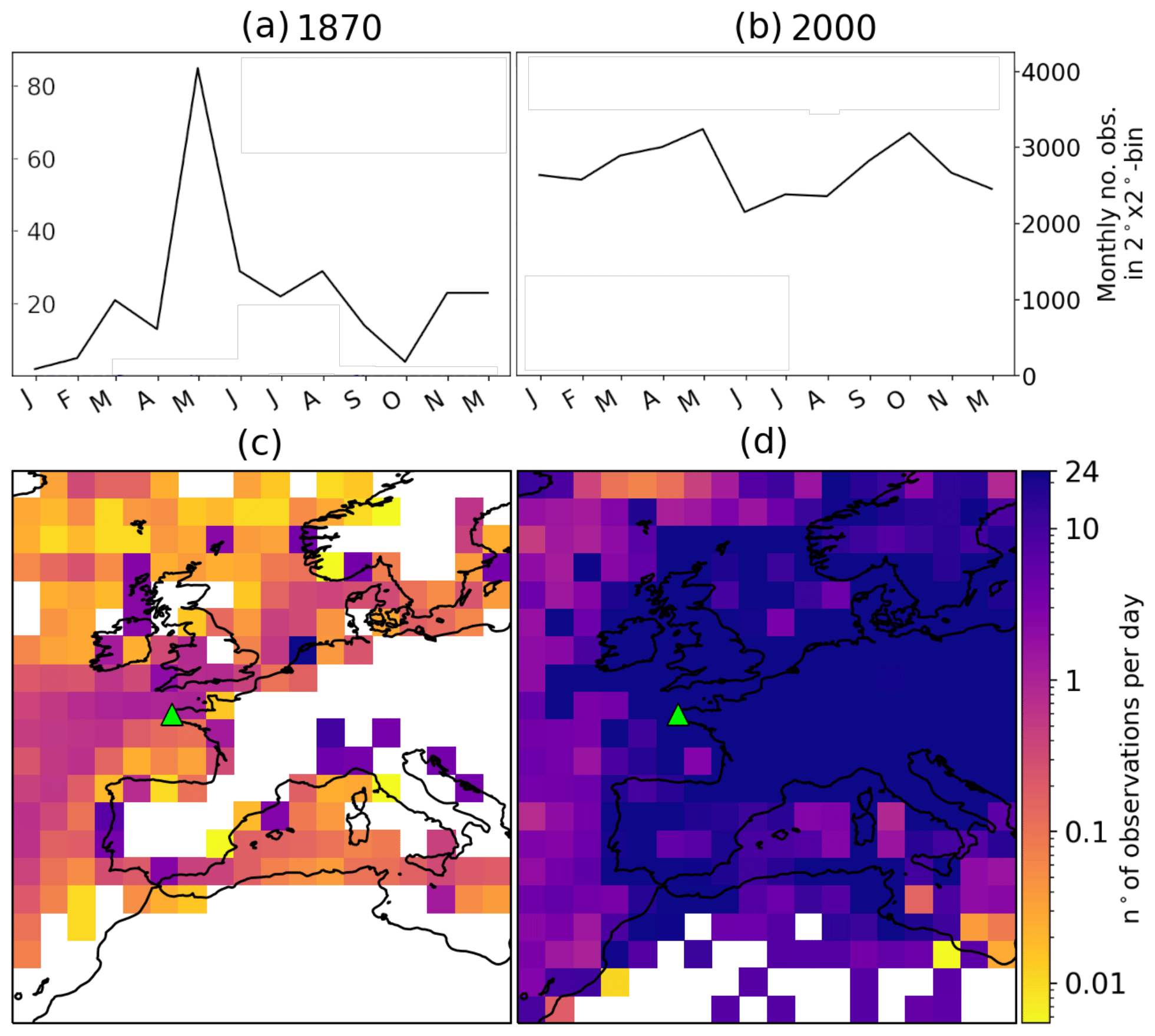
Figure 1 Number of surface pressure observations from the International Surface Pressure Databank (ISPD) assimilated in the 20th century Reanalysis version 3 (20CRv3). (a, b) Monthly count over a 2°×2° box centered on Brest for the years 1870 (a) and 2000 (b). (c, d) The yearly average of daily number of observation in 1870 (c) and 2000 (d).

The surface pressure observation density is considerably lower in the 19th century than in the late 20th century. An online platform (https://psl.noaa.gov/data/20CRv3_ISPD_obscounts_bymonth, last access: July 2024) allows us to consult the monthly observation count per 2°×2° box. Figure 1 shows yearly averages of the number of surface pressure observations per day, comparing the years 1870 and 2000. The maximum value was set to 24 observations per day, although in 2000 this value is mostly exceeded. In 1870, approximately half of Europe's land surface has no observations at all, and fewer than 10 points have more than 10 observations per day. Observations coming from ships allow us to raise the number of observations to approximately one per day in densely trafficked areas. Conversely, in 2000 virtually all of western Europe's land area has more than 24 observations per day. Taking a spatial average over the whole map from Fig. 1 gives approximately 1 observation every 3 d in 1870 versus 44 observations per day in 2000. The number of available observations is also highly variable through time, especially in the 19th century. For instance, in the 2°×2° box centered on 49° latitude, −5° longitude, the number of monthly observations in 1870 ranges from 2 (January 1870) to 85 (May 1870), while in 2000 it ranges from 2152 (June 2000) to 3242 (May 2000).

2.2 Preprocessing of mean sea level pressure

In this work, we only use the mean sea level pressure (MSLP) variable from 20CRv3. We perform two different preprocessing steps on this variable.

The first preprocessing step is used for the statistical relationship between the local pressure and the surge residual. As the latter is driven in part by a physical phenomenon called the inverse barometer effect, which will be introduced in the next section, we consider the difference between the MSLP interpolated at the city of Brest (48.3829° N, 4.49504° W) and the MSLP averaged over all members of 20CRv3 and over the North Atlantic Ocean (using the reanalysis' land mask and averaging from 0 to 69° N and from 98° W to 12° E), in a similar fashion to Ponte (1994). This spatially averaged pressure is denoted as ${\stackrel{\mathrm{‾}}{\mathrm{MSLP}}}^{\mathrm{ocean}}\left(t\right)$ and depends only on time. Note that there is a small variability in ocean-averaged pressure between 20CRv3 members in the 19th century. However, we have checked that this variability is 1 order of magnitude smaller than the inter-member variability of MSLP at the city of Brest, which justifies our approximation of using simply the member average of the ocean-averaged pressure as a reference.

A second preprocessing step of MSLP is used to compute the probability of transition from one member of the reanalysis to another in the hidden Markov model (HMM) presented in Sect. 3.2. For this purpose, we consider seasonal anomalies of MSLP with respect to a climatology computed from the period 1847–1890 because the HMM is run only for those years. The reference MSLP climatology for calendar day d and hour h is given by the average over days between d−30 and d+30, hours between h−3 and h+3, and all years 1847–1890. This reference MSLP is denoted as ${\stackrel{\mathrm{‾}}{\mathrm{MSLP}}}^{\mathrm{clim}}$ and depends on latitude and longitude.

2.3 Tide gauge of Brest (France)

In this study, the tide gauge of Brest is used as indirect tracer of atmospheric circulation through surge residuals. The Brest sea level record is taken from the GESLA-3 database starting in 1846 with hourly sampling. Apart from a few large gaps, the record is mostly continuous during periods 1847–1945 and 1953–present. This combination of historical and modern records is at the foundation of the methodology explored in the next section.

2.4 Preprocessing of sea level

As mentioned earlier, the part of the sea level that responds to atmospheric processes is the surge residual (see definition in Gregory et al., 2019). To access the surge residual, one has to remove the tidal part of the signal. Following this, as we are interested in sub-seasonal variations, we also remove the yearly variations in the mean sea level (at interannual and decadal scales), such as sea level rise (Cazenave and Llovel, 2010). In this work, we also use moving averages and differences in the surge residual. All of these steps are exemplified in Fig. 2.

Figure 2 An example output of the different stages of preprocessing of the sea level signal used in this work. (a) Sea level before (solid blue line) and after (dashed orange line) removing the tidal part of the signal. (b) Zero-median surge residual h(t) (1 h sampling, dashed orange curve), centered 12 h average ${\stackrel{\mathrm{‾}}{h}}^{\mathrm{1}\mathrm{h}}\left(t\right)$ (solid green curve), and the 12 h difference between 3 h averages of the surge residual $\mathrm{\Delta }{\stackrel{\mathrm{‾}}{h}}^{\mathrm{3}\mathrm{h}}\left(t\right)$ (dotted gray curve).

We first compute the tidal constituents of the raw sea level (blue curve, Fig. 2a) using U-Tide (Codiga, 2011), which performs harmonic (Fourier) decomposition with prescribed frequencies corresponding to planetary movements. The tidal constituents are computed over two different periods: 1847–1890 and 1981–2015. Removing the tidal part of the signal gives the surge residual (dashed orange line in Fig. 2a), which has a temporal average value of ∼4 m for the Brest tide gauge.

Following this, we remove the yearly median value of the sea level ( dashed orange line in Fig. 2b). We choose to remove the median and not the mean because the mean can in principle be influenced by the number and magnitude of extremes in a given year, which can be linked to the number and magnitude of storms passing in a given year. This second step allows us to access the zero-median surge residual which is denoted as h(t) in the following equation:

$$\begin{array}{}\text{(1)}& h\left(t\right)=H\left(t\right)-{\mathrm{Tide}}_H\left(t\right)-\mathrm{median}\left[H\right(t^{\prime }),t^{\prime }\in \mathrm{year}(t\left)\right],\end{array}$$

where H(t) denotes the raw sea level, Tide_H(t) is the tidal part of the signal computed from H, and year(t) is the year in which time t is found.

Note from Fig. 2b that the surge residual fluctuates at an hourly scale, part of which is due to oscillations that are not due to variations in atmospheric pressure. For instance, these oscillations can be due to tide–surge interactions (Horsburgh and Wilson, 2007) or measurement errors in the 19th century leading to phase shifts. Such 12 h oscillations can dominate the surge residual signal in Brest, where the tidal amplitude is large (see, for instance, 29 and 30 January 2014, Fig. 2). Furthermore, tide–surge interactions lead to stronger surge residuals at low tide and weaker surge residuals at high tide (Horsburgh and Wilson, 2007). As these phenomena are not linked to atmospheric processes, we chose to filter them out with a simple 12 h average (solid green curve in Fig. 2). Given the spatial resolution of 20CRv3, smaller-scale events are likely to not be represented in the MSLP fields used in this study. In the following, we denote the 12 h average of the zero-median surge residual as ${\stackrel{\mathrm{‾}}{h}}^{\mathrm{12}\mathrm{h}}\left(t\right)$, which is calculated using the following equation:

$$\begin{array}{}\text{(2)}& {\stackrel{\mathrm{‾}}{h}}^{\mathrm{12}\mathrm{h}}\left(t\right)={\displaystyle \frac{\mathrm{1}}{\mathrm{12}}}\sum _{t^{\prime }=-\mathrm{6}}^{t^{\prime }=+\mathrm{6}}h(t+t^{\prime }).\end{array}$$

Finally, note that if atmospheric pressure variations are faster than the typical time of adjustment of sea level, one expects deviations from the inverse barometer approximation (Bertin, 2016). Therefore, fast time variations in the surge residual are also expected, statistically speaking, to be associated with deviations from the inverse barometer approximation. To allow the model described in Sect. 3.1 to capture this effect, we compute the difference between the surge at time t and at time t−12 h, choosing the 12 h interval again to filter out oscillations at a period close to 12 h. Furthermore, since the reanalysis is run at 3 h resolution, we perform a 3 h moving average of the surge residual before computing the difference. This difference is denoted $\mathrm{\Delta }{\stackrel{\mathrm{‾}}{h}}^{\mathrm{3}\mathrm{h}}\left(t\right)$ and defined by the following equation:

$$\begin{array}{}\text{(3)}& \mathrm{\Delta }{\stackrel{\mathrm{‾}}{h}}^{\mathrm{3}\mathrm{h}}\left(t\right):={\displaystyle \frac{\mathrm{1}}{\mathrm{3}}}\sum _{t^{\prime }=-\mathrm{2}}^{t^{\prime }=+\mathrm{1}}\left[h\right(t+t^{\prime })-h(t-\mathrm{12}+t^{\prime }\left)\right].\end{array}$$

2.5 Independent historical pressure observations

In Sect. 5, we use pressure observations for the city of Brest and compare them with 20CRv3 and our estimate of pressure based on tide gauge observations and our statistical model (local linear regression, LLR). We downloaded these observations from a repository (https://github.com/ed-hawkins/weather-rescue-data/tree/main, last access: July 2024) gathering historical pressure observations. These pressure observations come from the EMULATE project (Ansell et al., 2006) for 1860–1880 and from Météo France archives for 1858–1860 and from 1880 on. The EMULATE dataset has a daily sampling, while the Météo France archive dataset has a daily to thrice-daily sampling. These observations were not included in 20CRv3, and we did not use them to tune our model, they thus provide an independent validation dataset.

We have found a shift in average pressure between the EMULATE and Météo France datasets. To overcome this issue, and since we are only interested in sub-seasonal atmospheric variability, we added a constant value of ∼0.22 hPa for the period 1860–1880 (EMULATE dataset) to each value of the independent pressure observation datasets so that the average pressure is equal between the independent observed pressure and the 20CRv3 mean pressure linearly interpolated at the city of Brest. We did the same operation for the period covered by the Météo France dataset that we are using (1855–1859 and 1881–1894), adding a value of ∼7.18 hPa.

3 Statistical methods

3.1 Local linear regression (LLR) between surge residuals and mean sea level pressure

To estimate the statistical relationship between surge residuals in Brest and 20CRv3 mean sea level pressure, we use the period 1981–2015, during which satellite data are used in 20CRv3 to constrain sea surface temperature and sea ice cover, and the large number of pressure observations gives us high confidence in the 20CRv3 fields of mean sea level pressure (MSLP).

The filtered surge residuals described in Sect. 2.4 respond to sub-seasonal variations in atmospheric pressure. First, the sea level is sensitive to pressure variations. An approximation called the “inverse barometer effect” (Roden and Rossby, 1999) states that an increase (decrease) of 1 hPa in pressure at the mean sea level leads to a decrease (increase) in sea level of approximately 1 cm. This approximation is valid only for slow variations in atmospheric pressure compared to the typical time of dynamic adjustment of the sea level (Bertin, 2016).

Moreover, the piling up of water due to wind blowing perpendicular to the coast is responsible for positive (negative) surge residuals when the wind stress transport is directed towards (away from) the coast. This effect depends nonlinearly on the wind amplitude and direction (Bryant and Akbar, 2016; Pineau-Guillou et al., 2018). Statistical anticorrelation observed in most regions between wind-driven and pressure-driven sea level fluctuations causes regressions of surge residual versus atmospheric pressure to deviate from the inverse barometer approximation (Ponte, 1994).

Since wind is not included in our model, the relationship between the filtered surge residuals and the atmospheric pressures from 20CRv3 should not be deterministic. It is also likely that typical wind conditions depend on the amplitude of the MSLP anomaly, meaning that the average value of MSLP anomaly for a given value of surge residual in Brest may be a nonlinear function. As shown by Hawkins et al. (2023), using a physical coastal model forced by the values of pressure (and wind) from the 20CR can lead to biases in the estimation of associated surges due to the resolution of the reanalysis. A statistical model can thus be used as a tool to correct such biases and represent uncertainties. In our case, since we want to estimate pressure based on the surge residuals only, the effect of unknown wind or other processes must also be taken into account through uncertainty quantification.

Since our predictor variable is the sea level measured by the tide gauge, we will use two proxies to estimate the conditional probability distribution of pressure: ${\stackrel{\mathrm{‾}}{h}}^{\mathrm{12}\mathrm{h}}\left(t\right)$ and $\mathrm{\Delta }{\stackrel{\mathrm{‾}}{h}}^{\mathrm{3}\mathrm{h}}\left(t\right)$. We expect that corresponding atmospheric pressure variations should be slow and moderate for low absolute values of these two predictors and that winds should be of low intensity, meaning that the inverse barometer approximation should hold. For larger absolute values of $\mathrm{\Delta }{\stackrel{\mathrm{‾}}{h}}^{\mathrm{3}\mathrm{h}}\left(t\right)$, indicating rapidly changing surge residuals and thus likely also rapidly changing atmospheric conditions, we expect deviations from the inverse barometer due to the dynamical adjustment of the sea level. Similarly, the largest absolute values of ${\stackrel{\mathrm{‾}}{h}}^{\mathrm{12}\mathrm{h}}\left(t\right)$ are likely to be caused by the added contribution of wind to the effect of pressure, meaning that deviations from the inverse barometer are expected as well.

To model all of these effects, we use a local linear regression (LLR in the following; see, e.g., Fan, 1993; Hansen, 2022), also called kernel regression (Takeda et al., 2007). More precisely, we borrow our LLR from Lguensat et al. (2017). In such a model, we will search for similar values (neighbors) of the two predictor variables ${\stackrel{\mathrm{‾}}{h}}^{\mathrm{12}\mathrm{h}}\left(t\right)$ and $\mathrm{\Delta }{\stackrel{\mathrm{‾}}{h}}^{\mathrm{3}\mathrm{h}}\left(t\right)$ in the whole dataset and compute a linear regression on this subset of the dataset. The predicted variable is $\mathrm{MSLP}\left(t\right)-{\stackrel{\mathrm{‾}}{\mathrm{MSLP}}}^{\mathrm{ocean}}\left(t\right)$, where MSLP(t) is the value of the MSLP linearly interpolated at the city of Brest from the reanalysis.

We will assume that, conditionally to the values of ${\stackrel{\mathrm{‾}}{h}}^{\mathrm{12}\mathrm{h}}\left(t\right)$ and $\mathrm{\Delta }{\stackrel{\mathrm{‾}}{h}}^{\mathrm{3}\mathrm{h}}\left(t\right)$, the predicted variable $\mathrm{MSLP}\left(t\right)-{\stackrel{\mathrm{‾}}{\mathrm{MSLP}}}^{\mathrm{ocean}}\left(t\right)$ follows a Gaussian distribution:

$$\begin{array}{}\text{(4)}& \mathrm{MSLP}\left(t\right)-{\stackrel{\mathrm{‾}}{\mathrm{MSLP}}}^{\mathrm{ocean}}\left(t\right)\sim \mathcal{N}\left(m\right(t),\mathrm{var}(t\left)\right).\end{array}$$

We then assume, following Lguensat et al. (2017), that the average m(t) and variance var(t) of this distribution can be estimated at each time step based on a local linear regression. To perform this local regression, we search for the k-nearest neighbors of [${\stackrel{\mathrm{‾}}{h}}^{\mathrm{12}\mathrm{h}}\left(t\right)$, $\mathrm{\Delta }{\stackrel{\mathrm{‾}}{h}}^{\mathrm{3}\mathrm{h}}\left(t\right)$] in the satellite era (1981–2015), where k is an integer set to 200 (other values have been tested and did not yield improvement on the results). The nearest-neighbor criterion is the Euclidean distance in the two-dimensional space of values of [${\stackrel{\mathrm{‾}}{h}}^{\mathrm{12}\mathrm{h}}\left(t\right)$, $\mathrm{\Delta }{\stackrel{\mathrm{‾}}{h}}^{\mathrm{3}\mathrm{h}}\left(t\right)$]. For each time t at which we want to estimate $\mathrm{MSLP}\left(t\right)-{\stackrel{\mathrm{‾}}{\mathrm{MSLP}}}^{\mathrm{ocean}}\left(t\right)$, we thus find the set of times $\mathit{\{}{t}_i,i\in I(t\left)\mathit{\right\}}$ where I(t) is an ensemble of size K, for which the following distance is minimal:

$$\mathrm{dist}\left(t,t_i\right)={\left[\left({\stackrel{\mathrm{‾}}{h}}^{\mathrm{12}\mathrm{h}}\left(t\right)-{\stackrel{\mathrm{‾}}{h}}^{\mathrm{12}\mathrm{h}}\left(t_i\right)\right)+{\left(\mathrm{\Delta }{\stackrel{\mathrm{‾}}{h}}^{\mathrm{3}\mathrm{h}}\left(t\right)-\mathrm{\Delta }{\stackrel{\mathrm{‾}}{h}}^{\mathrm{3}\mathrm{h}}\left(t_i\right)\right)}^{\mathrm{2}}\right]}^{\mathrm{1}/\mathrm{2}}.$$

We attach a weight ω_i(t) to each index i∈I(t) according to the following formula:

$$\begin{array}{}\text{(5)}& {\mathit{\omega }}_i\left(t\right)={\displaystyle \frac{\exp \left(-\mathrm{dist}{\left(t,t_i\right)}^{\mathrm{2}}/\mathit{\lambda }(t{)}^{\mathrm{2}}\right)}{\sum _{j\in I\left(t\right)}\exp \left(-\mathrm{dist}{\left(t,t_j\right)}^{\mathrm{2}}/\mathit{\lambda }(t{)}^{\mathrm{2}}\right)}},\end{array}$$

where $\mathit{\lambda }\left(t\right):=\mathrm{median}\mathit{\left\{}\mathrm{dist}\right(t,t_i),i\in I(t\left)\mathit{\right\}}$ is defined as the median of the local values of the distances to the nearest neighbors (Lguensat et al., 2017).

Using this subset of the whole dataset, we compute a weighted linear regression between the subset of regressors ${\stackrel{\mathrm{‾}}{h}}^{\mathrm{12}\mathrm{h}}\left(t_i\right)$, $\mathrm{\Delta }{\stackrel{\mathrm{‾}}{h}}^{\mathrm{3}\mathrm{h}}\left(t_i\right)$ and of the predicted variable $\mathrm{MSLP}\left(t_i\right)-{\stackrel{\mathrm{‾}}{\mathrm{MSLP}}}^{\mathrm{ocean}}\left(t_i\right)$ using the weights ω_i(t). This regression has two linear coefficients denoted as  α(t) and β(t) and one intercept (constant value) denoted as γ(t). Following this, the average is given by applying the local weighted linear model to the actual value of the predictors:

$$\begin{array}{}\text{(6)}& m\left(t\right)=\mathit{\alpha }\left(t\right){\stackrel{\mathrm{‾}}{h}}^{\mathrm{12}\mathrm{h}}\left(t\right)+\mathit{\beta }\left(t\right)\mathrm{\Delta }{\stackrel{\mathrm{‾}}{h}}^{\mathrm{3}\mathrm{h}}\left(t\right)+\mathit{\gamma }\left(t\right),\end{array}$$

while the variance is given by the weighted variance of the prediction error from the weighted linear model over the set of nearest neighbors:

$$\begin{array}{}\text{(7)}& \begin{array}{rl}\mathrm{var}\left(t\right)=& {\displaystyle \frac{\mathrm{1}}{\mathrm{1}-\sum _{i\in I\left(t\right)}{\mathit{\omega }}_i(t{)}^{\mathrm{2}}}}\sum _{i\in I\left(t\right)}{\mathit{\omega }}_i\left(t\right)\\ & \left(\mathrm{MSLP}\left(t_i\right)-{\stackrel{\mathrm{‾}}{\mathrm{MSLP}}}^{\mathrm{ocean}}\left(t_i\right)-\mathit{\alpha }\left(t\right){\stackrel{\mathrm{‾}}{h}}^{\mathrm{12}\mathrm{h}}\left(t_i\right)\right.\\ & {\left.-\mathit{\beta }\left(t\right)\mathrm{\Delta }{\stackrel{\mathrm{‾}}{h}}^{\mathrm{3}\mathrm{h}}\left(t_i\right)-\mathit{\gamma }\left(t\right)\right)}^{\mathrm{2}}.\end{array}\end{array}$$

To test the accuracy of this model on the 1980–2015 period, we apply it for all times t∈[1980–2015], searching for neighboring times t_i in the same period but with the condition that there is a minimum of 2 weeks between t and t_i (i.e., excluding the interval [t−14 d, t+14 d]). This is called the leave-one-out procedure, ensuring that the data that are used to fit the model do not include the true values. Following this, we compare the average m(t) with the true value $\mathrm{MSLP}\left(t\right)-{\stackrel{\mathrm{‾}}{\mathrm{MSLP}}}^{\mathrm{ocean}}\left(t\right)$ in a scatterplot (Fig. 3a). This figure shows that the LLR is able to predict good average values m(t) for moderate absolute values of pressure difference, although it consistently underestimates the most extreme values: this behavior is expected as the method is limited by the observations it has seen previously. However, as will be seen in Sect. 5, this simple model is still able to capture storms. Following this, we test the adequacy of our variability estimate with the parameter var(t) by checking that the following shifted and rescaled variable follows a standard Gaussian distribution with an average of 0 and variance of 1:

$$\begin{array}{}\text{(8)}& {\displaystyle \frac{\mathrm{MSLP}\left(t\right)-{\stackrel{\mathrm{‾}}{\mathrm{MSLP}}}^{\mathrm{ocean}}\left(t\right)-m\left(t\right)}{\sqrt{\mathrm{var}\left(t\right)}}}.\end{array}$$

To do so, we compare the empirical histogram of this variable with the probability density function of a standard Gaussian distribution, as shown in Fig. 3b. Although the shape of the histogram slightly differs from a Gaussian probability density function (it is more peaked and has heavier tails), the agreement is satisfying enough for the purpose of this article. This shows that the estimate of variance through var(t) is consistent with the real variability of the estimation process, which is the reason why we advocate for using a statistical method in the first place.

Figure 3 Evaluation of the local linear regression (LLR) on the period 1981–2015 using a leave-one-out procedure. (a) Histogram scatterplot of the average estimate from the LLR versus the true value of the MSLP difference with the reference ocean-averaged MSLP. (b) Density histogram of normalized average error of the LLR estimate (black line) compared to theoretical probability density function of the standard Gaussian random variable (dashed orange line).

3.2 Hidden Markov model (HMM)

In the 19th century, the spread between 20CRv3 members is much larger than in the period 1981–2015. One of the aims of this work is to estimate conditional probabilities of each member of the reanalysis based on surge residuals in Brest. Note that in the reanalysis the members are assumed to have uniform probabilities, i.e., a probability of $\mathrm{1}/\mathrm{80}$, as we have 80 members.

One can estimate conditional probabilities of each member at time t based on the values of [${\stackrel{\mathrm{‾}}{h}}^{\mathrm{12}\mathrm{h}}\left(t\right)$, $\mathrm{\Delta }{\stackrel{\mathrm{‾}}{h}}^{\mathrm{3}\mathrm{h}}\left(t\right)$]. To do that, we use the satellite-era-derived local linear regression expressed in Sect. 3.1. The average m(t) and variance var(t) are estimated based on the procedure described in Sect. 3.1 and using the dataset from the period 1981–2015 to search for neighbors of [${\stackrel{\mathrm{‾}}{h}}^{\mathrm{12}\mathrm{h}}\left(t\right)$, $\mathrm{\Delta }{\stackrel{\mathrm{‾}}{h}}^{\mathrm{3}\mathrm{h}}\left(t\right)$] and compute the LLR.

To differentiate these member probabilities from the ones we will derive later on using a hidden Markov model, we use the notation $p_{\cancel{\mathrm{HMM}}}(i,t)$ for the probability of member i at time t.

$$\begin{array}{}\text{(9)}& \left\{\begin{array}{l}{p}_{\cancel{\mathrm{HMM}}}(i,t)\propto \exp \left\{-\frac{{\left(\mathrm{MSLP}(i,t)-{\stackrel{\mathrm{‾}}{\mathrm{MSLP}}}^{\mathrm{ocean}}\left(t\right)-m\left(t\right)\right)}^{\mathrm{2}}}{\mathrm{2}\mathrm{var}\left(t\right)}\right\},\\ \sum _{i=\mathrm{1}}^{\mathrm{80}}{p}_{\cancel{\mathrm{HMM}}}(i,t)=\mathrm{1}\end{array}\right.\end{array}$$

We also use the convention that, in the absence of surge residuals observations, all members are given equal probabilities $p_{\cancel{\mathrm{HMM}}}(i,t)=\mathrm{1}/\mathrm{80}$. Although these probabilities already bear significant information, they have the undesirable property of being time-discontinuous. This is not coherent with the fact that the members of 20CRv3 are time-continuous: they are propagated in time using a Numerical Weather Prediction (NWP) model. To remedy this issue, we compute smoothed (or reanalyzed) probabilities using a hidden Markov model (HMM) detailed below, which we write as p_HMM(i,t):

$$\begin{array}{}\text{(10)}& p_{\mathrm{HMM}}(i,t):=P\left(\mathrm{member}\left(t\right)=i\mathrm{|}\left[\begin{array}{c}H(t=\mathrm{1})\\ \mathrm{⋮}\\ H(t=T)\end{array}\right]\right),\end{array}$$

where one uses an observational record of surge residuals from time index 1 to T, and we use the simple notation $H\left(t\right):=\left[{\stackrel{\mathrm{‾}}{h}}^{\mathrm{12}\mathrm{h}}\right(t),\mathrm{\Delta }{\stackrel{\mathrm{‾}}{h}}^{\mathrm{3}\mathrm{h}}(t\left)\right]$ for the vector of surge residual average and difference. Here, p_HMM(i,t) is a time-smoothed version of $p_{\cancel{\mathrm{HMM}}}(i,t)$ that takes into account past and future values of the surge residual. For this purpose, a simple hidden Markov model (HMM) is used. The first ingredient of the HMM is the transition matrix T_ij(t) from member i at time t−1 to member j at time t.

$$\begin{array}{}\text{(11)}& {\mathbf{T}}_{ij}\left(t\right):=P\left(\mathrm{member}\right(t)=j\mathrm{|}\mathrm{member}(t-\mathrm{1})=i)\end{array}$$

To estimate the transition matrix, a strong hypothesis is made:

$$\begin{array}{}\text{(12)}& {\mathbf{T}}_{ij}\left(t\right)\propto K_{\mathit{\theta }}\left({\mathrm{MSLP}}_{\mathrm{map},j}\left(t\right),{\mathrm{MSLP}}_{\mathrm{map},i}\left(t\right)\right),\end{array}$$

where MSLP_map,i(t) is the ith member's map of mean sea level pressure in a squared box (28° N ≤ lat ≤ 64° N, 18° W ≤ long ≤ 18° E) at time t and $K_{\mathit{\theta }}(\cdot ,\cdot )$ is a positive real-valued function that measures the similarity between MSLP_map,i(t) and MSLP_map,j(t) and depends on the parameter θ.

Equation (12) states that transitions from one member to another are more likely if the associated MSLP maps at time t are similar. This prevents abrupt transitions to dissimilar atmospheric states. The size and location of the map was chosen to cover an area inside which storms and anticyclones that affect the surge residuals in Brest would lie. Ideally, $K_{\mathit{\theta }}(\cdot ,\cdot )$ should be symmetric and semi-definite. Here, a simple Gaussian kernel of Euclidean distances is used, with normalization factor θ>0, meaning that for two fields X and Y:

$$\begin{array}{}\text{(13)}& K_{\mathit{\theta }}(X,Y)=\exp \left\{-\sum _{n\in \mathrm{lons}}\sum _{l\in \mathrm{lats}}{\displaystyle \frac{{\left(X_{nl}-Y_{nl}\right)}^{\mathrm{2}}}{{\mathit{\theta }}^{\mathrm{2}}}}\right\},\end{array}$$

where the sum over n and l represents a sum over longitudes and latitudes. We then define Θ through the following equation:

$$\begin{array}{}\text{(14)}& {\displaystyle \frac{\mathit{\theta }}{\mathrm{\Theta }}}=\stackrel{\mathrm{‾}}{{\left({\displaystyle \frac{\mathrm{1}}{\mathrm{80}}}\sum _{i=\mathrm{1}}^{\mathrm{80}}{\displaystyle \frac{\mathrm{1}}{T}}\sum _{t=\mathrm{0}}^T{\mathrm{MSLP}}_{\mathrm{map},i}(t{)}^{\mathrm{2}}\right)}^{\mathrm{1}/\mathrm{2}}},\end{array}$$

where the overbar denotes spatial average. This normalization will allow us to optimize θ through a grid search of Θ for a maximum likelihood of the surge residual observations.

One can compute T_ij(t) by setting a value of θ and using the hypothesis of Eq. (12), along with the fact that for all i and t we have $\sum _j{\mathbf{T}}_{ij}\left(t\right)=\mathrm{1}$. This then allows us to estimate p_HMM(i,t) with the forward–backward algorithm (Rabiner, 1989).

$$\begin{array}{}\text{(15)}& {\displaystyle }& {\displaystyle }{a}_i\left(t\right):=P\left(\left[\begin{array}{c}H\left(\mathrm{1}\right)\\ \mathrm{⋮}\\ H\left(t\right)\end{array}\right],\mathrm{member}\left(t\right)=i\right),\text{(16)}& {\displaystyle }& {\displaystyle }{b}_i\left(t\right):=P\left(\left[\begin{array}{c}H(t+\mathrm{1})\\ \mathrm{⋮}\\ H\left(T\right)\end{array}\right]\mathrm{|}\mathrm{member}\left(t\right)=i\right).\end{array}$$

These two quantities can be computed recursively, following the forward procedure:

$$\begin{array}{}\text{(17)}& {\displaystyle }& {\displaystyle }{a}_i\left(\mathrm{1}\right)=p_{\cancel{\mathrm{HMM}}}(i,\mathrm{1}),\text{(18)}& {\displaystyle }& {\displaystyle }{a}_i(t+\mathrm{1})=p_{\cancel{\mathrm{HMM}}}(i,t+\mathrm{1})\sum _{j=\mathrm{1}}^{\mathrm{80}}{a}_j\left(t\right){\mathbf{T}}_{ji}\left(t\right),\end{array}$$

and the backward procedure:

$$\begin{array}{}\text{(19)}& {\displaystyle }& {\displaystyle }{b}_i\left(T\right)=\mathrm{1},\text{(20)}& {\displaystyle }& {\displaystyle }{b}_i\left(t\right)=\sum _{j=\mathrm{1}}^{\mathrm{80}}{b}_j(t+\mathrm{1}){\mathcal{T}}_{ij}\left(t\right)p_{\cancel{\mathrm{HMM}}}(j,t+\mathrm{1}).\end{array}$$

Finally, this allows us to estimate p_HMM(i,t) by noting that

$$\begin{array}{}\text{(21)}& p_{\mathrm{HMM}}(i,t)={\displaystyle \frac{P\left(\mathrm{member}\left(t\right)=i,\left[\begin{array}{c}{H}_{\mathrm{1}}\\ \mathrm{⋮}\\ H_T\end{array}\right]\right)}{P\left(\left[\begin{array}{c}{H}_{\mathrm{1}}\\ \mathrm{⋮}\\ H_T\end{array}\right]\right)}},\end{array}$$

which gives, in terms of a_i(t) and b_i(t):

$$\begin{array}{}\text{(22)}& p_{\mathrm{HMM}}(i,t)={\displaystyle \frac{a_i\left(t\right)b_i\left(t\right)}{\sum _{j=\mathrm{1}}^{\mathrm{80}}{a}_j\left(t\right)b_j\left(t\right)}},\end{array}$$

while keeping in mind that Eq. (22) implicitly relies on hypothesis (Eq. 12) and a fixed form of K_θ.

Comparing p_HMM(i,t) with the uniform distribution $p(i,t)=\frac{\mathrm{1}}{\mathrm{80}}$ allows us to see if the surge residual observations are coherent with the MSLP fields of 20CRv3 (Sect. 4) and to select the most relevant members given surge residual data (Sect. 5).

To choose the parameter θ, we performed a grid search of its normalized form Θ and computed the log likelihood of the surge residual observations as an output of the algorithm. Indeed, the log likelihood l_θ(0 … T) is expressed as follows:

$$\begin{array}{}\text{(23)}& l_{\mathit{\theta }}\left(\mathrm{0}\mathrm{\dots }T\right)=\log \left(\sum _{i=\mathrm{1}}^{\mathrm{80}}{a}_i\left(T\right)\right).\end{array}$$

Figure 4 shows variations in this quantity with Θ for 1 year (1885) of surge residual observations in Brest (i.e., t=0 is 1 January 1885, while T is 1 January 1886). The curve shows a distinct maximum around Θ≈0.09 and plateaus for higher values. According to Fig. 4, the difference in log likelihood between the model without HMM ($\mathit{\theta }=+\mathrm{\infty }$) and with HMM is close to 1000. The introduction of one extra parameter in the filtering model compared to the static one is thus clearly justified if the two models are compared using standard criteria such as the Akaike information criterion (AIC), the Bayesian information criterion (BIC), or likelihood ratio tests (Zucchini et al., 2017).

Figure 4 Log likelihood of Brest surge residuals (dotted blue line) as a function of parameter Θ defined in Eq. (14). For comparison, the log likelihood of the simple model without the hidden Markov model ($\mathrm{\Theta }\to +\mathrm{\infty }$) is also shown (dashed gray line). The log likelihood was estimated using data from year 1885 for a first estimation of optimal parameter Θ. Values of Θ used for estimation are 0.02, 0.04, 0.05, 0.06, 0.07, 0.08, 0.09, 0.1, 0.11, 0.13, 0.15, 0.2, 1, and 10, with 0.07 giving the largest log likelihood.

Note that in the limit $\mathrm{\Theta }=+\mathrm{\infty }$, we have a constant transition probability ${\mathbf{T}}_{ij}\left(t\right)=\frac{\mathrm{1}}{\mathrm{80}}$, and p_HMM(i,t) reduces to $p_{\cancel{\mathrm{HMM}}}(i,t)$. Figure 4 thus supports the use of the HMM to estimate probabilities of the MSLP map conditioned by surge residual observations.

The choice of restricting the estimation of log likelihood to one arbitrary year (1885) is supported by the fact that estimation of T_ij(t) is computationally expansive. We assume that the optimal value of θ generalizes well to other years. A better optimization of θ would necessitate further work that is out of the scope of this study. Setting Θ=0.09 will already enable us to find interesting features of p_HMM(i,t).

4 Modification of 20CRv3 ensemble when accounting for surge residuals

This section is devoted to the study of δμ_HMM(t), the difference between weighted and unweighted ensemble average, defined by

$$\begin{array}{}\text{(24)}& \mathit{\delta }{\mathit{\mu }}_{\mathrm{HMM}}\left(t\right):=\sum _{i=\mathrm{1}}^{\mathrm{80}}\left(p_{\mathrm{HMM}}(i,t)-{\displaystyle \frac{\mathrm{1}}{\mathrm{80}}}\right){\mathrm{MSLP}}_{\mathrm{map},i}\left(t\right),\end{array}$$

where MSLP_map,i(t) is a short notation for the sea level pressure field of 20CRv3's ith member. Here, $\mathit{\delta }{\mathit{\mu }}_{\cancel{\mathrm{HMM}}}\left(t\right)$ is defined equivalently using $p_{\cancel{\mathrm{HMM}}}(i,t)$. This quantity shows how strong the average deviation is when taking into account surge residual observations. It will also sometimes be normalized by σ_20CR(t), the estimated standard deviation of the unweighted ensemble:

$$\begin{array}{}\text{(25)}& \begin{array}{rl}& {\mathit{\sigma }}_{\mathrm{20}\mathrm{CR}}\left(t\right):=\\ & {\left[{\displaystyle \frac{\mathrm{1}}{\mathrm{79}}}\sum _{i=\mathrm{1}}^{\mathrm{80}}{\left({\mathrm{MSLP}}_{\mathrm{map},i}\left(t\right)-{\displaystyle \frac{\mathrm{1}}{\mathrm{80}}}\sum _{i=\mathrm{1}}^{\mathrm{80}}{\mathrm{MSLP}}_{\mathrm{map},i}\left(t\right)\right)}^{\mathrm{2}}\right]}^{\mathrm{1}/\mathrm{2}}.\end{array}\end{array}$$

Note that in this definition σ_20CR(t) depends on time, latitude, and longitude. Therefore, at each grid point and for each time step the quantity δμ_HMM(t) will be normalized by a different value, indicating the strength of the reanalysis ensemble spread at this location in time and space.

To further interpret the result of our HMM algorithm, we introduce the filtered effective ensemble size ν_HMM(t) (Liu, 1996):

$$\begin{array}{}\text{(26)}& {\mathit{\nu }}_{\mathrm{HMM}}\left(t\right):={\displaystyle \frac{\mathrm{1}}{\sum _{i=\mathrm{1}}^{\mathrm{80}}{p}_{\mathrm{HMM}}(i,t{)}^{\mathrm{2}}}},\end{array}$$

and we equivalently define ${\mathit{\nu }}_{\cancel{\mathrm{HMM}}}\left(t\right)$. These quantities are estimates of the number of ensemble members that can be retained according to surge residual observations, assuming one discards very unlikely members.

Figure 5 (a) Average MSLP deviation δμ_HMM in pascals in the center of the Bay of Biscay. Panel (b) is the same as panel (a) but normalized by reanalysis ensemble standard deviation $\mathit{\delta }{\mathit{\mu }}_{\mathrm{HMM}}/{\mathit{\sigma }}_{\mathrm{20}\mathrm{CR}}$. (c) Effective ensemble size ν_HMM. Orange is used for data using smoothed probabilities with HMM p_HMM(i,t). Blue is used for data using probabilities without HMM $p_{\cancel{\mathrm{HMM}}}(i,t)$. Bold lines indicate yearly average. Thin lines indicate the 3-month average. All plots make simultaneous use of data from the Brest tide gauge.

In Fig. 5, the variables δμ_HMM, $\mathit{\delta }{\mathit{\mu }}_{\mathrm{HMM}}/{\mathit{\sigma }}_{\mathrm{20}\mathrm{CR}}$, and ν_HMM are shown as a function of time for the period 1846–1890. All these quantities show a strong seasonality. This is due to a much stronger MSLP variability in winter and a corresponding stronger response of the surge residuals. The figure shows that the amount of correction δμ_HMM and the decrease in ensemble size ν_HMM are much stronger using smoothed probabilities with HMM rather than probabilities without HMM. Showing the deviation δμ_HMM in the Bay of Biscay, where the standard deviation of $\mathit{\delta }{\mathit{\mu }}_{\mathrm{HMM}}/{\mathit{\sigma }}_{\mathrm{HMM}}$ is strongest (see Fig. 6), substantial absolute values of ∼600 Pa are obtained in early 1850s winters, even after averaging over 3 months. These large deviations correspond to more than 1 standard deviations of the ensemble size. Using probabilities without HMM, deviations are weaker but still non-negligible (∼500 Pa, ∼0.7σ). The slow decrease in δμ_HMM with time is coherent with slowly increasing observations used in 20CRv3, albeit with substantial decadal variations. However, $\mathit{\delta }{\mathit{\mu }}_{\cancel{\mathrm{HMM}}}/{\mathit{\sigma }}_{\mathrm{HMM}}$ and $\mathit{\delta }{\mathit{\mu }}_{\mathrm{HMM}}/{\mathit{\sigma }}_{\mathrm{HMM}}$ do not show a clear trend, indicating a persisting gain in information from surge residual observations throughout the 19th century.

Figure 6 Time standard deviation of $\mathit{\delta }{\mathit{\mu }}_{\cancel{\mathrm{HMM}}}$ (a, d), δμ_HMM (b, e), and $\mathit{\delta }{\mathit{\mu }}_{\mathrm{HMM}}/{\mathit{\sigma }}_{\mathrm{20}\mathrm{CR}}$ (c, f) computed from October to March for the years 1848–1880 (a–c) and 1880–1890 (d–f). Probabilities $p_{\cancel{\mathrm{HMM}}}$ and p_HMM make use of data from the Brest tide gauge.

In terms of effective size, Fig. 5 shows that the smoothing HMM algorithm imposes a strong member selection, with mostly only one member retained at each time step in winter and before 1880. Probabilities without HMM mostly retain more than half of the members, although peak low values of ${\mathit{\nu }}_{\cancel{\mathrm{HMM}}}\left(t\right)$ show that even without the HMM sometimes more than half of the ensemble members are highly unlikely. Filtered effective ensemble size reaches very low yearly and seasonal average values, indicating that many 20CR members are highly unlikely with respect to surge residual estimates from tide gauge observations. A strong increase in ν_HMM(t) is witnessed around year 1880. This can be explained by the availability of a large number of weather station data in eastern Europe and Russia from 1880 on and by an intensification of maritime traffic around 1880.

Figure 7 The bold orange line shows the yearly average of δμ_HMM at 47.83° latitude and −7.57° longitude in the Bay of Biscay using data from the Brest tide gauge. The thin black line shows the zero-median Brest surge residual (inverted sign).

The spatial structure of δμ is examined in Fig. 6. The analysis of time standard deviation of $\mathit{\delta }{\mathit{\mu }}_{\cancel{\mathrm{HMM}}}$ and $\mathit{\delta }{\mathit{\mu }}_{\mathrm{HMM}}/{\mathit{\sigma }}_{\mathrm{20}\mathrm{CR}}$ shows that the area of greatest influence of the corrections from surge residual smoothing from Brest tide gauge is in the Bay of Biscay. This can be explained by the passage of strong storms in the Bay of Biscay, which can cause high surge residuals in Brest, and by the sparsity of direct pressure measurements (ship logs) in this area in the 19th century. The standard deviation of δμ_HMM shows the largest values to the northwest of the map, which is where strong storms travel. Indeed, the variability of MSLP shows a great northwest gradient, as can be seen from maps of time standard deviation of 20CRv3 mean MSLP (not shown). Noticeably, the size of the area of influence of δμ_HMM is smaller in 1880–1890, which can be explained by a greater conditioning of 20CRv3 members by observations both offshore and inland. In cases of very sparse observations used in 20CRv3, the area of influence of these corrections widens due to continuity of MSLP fields. Note also that the area of influence is greater for δμ_HMM then for $\mathit{\delta }{\mathit{\mu }}_{\cancel{\mathrm{HMM}}}$ because of the time propagation of corrections thanks to the smoothing HMM algorithm. Finally, Fig. 6 confirms the large difference in amplitude of deviations between pre-1880 and post-1880 corrections already witnessed in Fig. 5. Similar spatial footprints can be witnessed from maps of high and low quantiles of δμ but with different values (not shown). Similarly, computing the time standard deviations as in Fig. 6 but restricting the times used for computation to April–September rather than October–March shows the same spatial pattern but with much lower values (not shown).

These corrections also have a strong decadal variation, with non-trivial yearly averages persisting for several years, as shown in Fig. 7. The same behavior can be witnessed for the surge residual, which is strongly anti-correlated to these deviations (Fig. 7). This can be explained by the fact that 20CRv3 smooths MSLP values in areas of sparse measurements and that surge residual filtering corrections allow us to retrieve more realistic intense values (either positive or negative). This interannual variability is related to the variability in storminess (Bärring and Fortuniak, 2009).

5 Focus on four 19th-century events

One of the aim of this study is to show that old tide gauge data can be used to better understand past severe storms. In this section, two storms and one mild situation are studied for illustrative purposes.

Figure 8 Comparison of MSLP estimation in Brest from 20CRv3 (blue), LLR based on surge residuals (orange), and independent observations (black dots) that were not used to build the orange and blue curves for three periods surrounding the events studied in this section. Full lines correspond to average values, while shaded areas correspond to ±1 SD (1 standard deviation) around the average.

To better understand the more general context of the three events studied in this section, we first look at longer time periods (100 d) surrounding the events and compare the results of the simple LLR based on surge residuals with 20CRv3 and independent observations (when available). These are plotted in Fig. 8. One can thus see that the uncertainties associated with the surge-residual-based LLR do not vary from year to year, while those of 20CRv3 decrease. More precisely, the ratio of the standard deviation of the LLR divided by that of 20CRv3 has an average value of 1.22 in 1847, 1.54 in 1865, 1.95 in 1876, and 2.45 in 1888. That same ratio has a minimum value of 0.47 both in 1847 and in 1865, while its minimum value is of 0.69 in 1876 and 0.94 in 1888. This shows that on average the reanalysis has lower uncertainty than the surge-residual-based pressure estimate (albeit with fluctuations), and in 1888 the uncertainty of the reanalysis is always smaller. Comparison with observations also confirms the better precision of the reanalysis.

In 1865 (Fig. 8b), although the surge-residual-based reconstruction is sometimes more consistent with observations than the reanalysis, there are as many occasions where it is the reanalysis that is more consistent with the independent observations. In 1876 (Fig. 8c), biases of ∼5 hPa between the LLR and 20CRv3 are found most of the time. For all four periods shown, the reanalysis and the LLR pressure estimates show consistent variations in time, albeit with persistent biases (either positive or negative) that last from a few days to ∼15 d. We attribute these biases to different atmospheric conditions that cannot be estimated from the surge residuals with our simple LLR model, in particular wind directions and intensity. These examples show that the results of our algorithm must be interpreted with care and that a more in-depth analysis is needed to understand the specifics of an individual event.

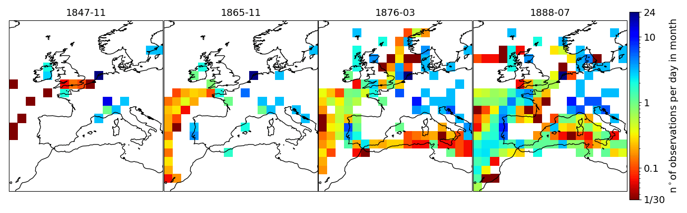
Figure 9 Number of pressure observations per month divided by 30 (or 31) to give an average number of observations per day for the months of November 1847, November 1865, March 1876, and July 1888.

Our claim that the wind variations are responsible for the persistent biases between the LLR pressure estimation and the reanalysis is supported by Fig. 12f, where we also show the direction and amplitude of the 10 m wind intensity as given by the average over all reanalysis members and interpolated at the city of Brest. In March 1876, two low-pressure systems passed to the north of Brest's tide gauge, the first around 10 March and second around 12 March, as indicated by the reanalysis members and the independent pressure observations (Fig. 12e). However, the first low-pressure system did not induce a surge residual as strong as the second one. One key difference between the two events is the wind amplitude, which reached 15 m s⁻¹ during the first event and then decreased to 5–10 m s⁻¹ during the second event, with almost steady wind direction. Although wind intensity and direction estimated from the reanalysis must be taken with care, the value of 15 m s⁻¹ is rarely exceeded (only 7 in 1000 times in the period 1981–2015, not shown), indicating exceptional wind intensity during the event and justifying the inaccuracy of the LLR, which is based on already observed events and therefore biased towards typical wind conditions. Our interpretation relies on the fact that the effect of wind on extreme surge residuals acts at small timescales (daily or sub-daily), which is backed by recent work (Pineau-Guillou et al., 2023).

To aid the interpretation of Figs. 10–13, in Fig. 9 we also show the number of observations assimilated in 20CRv3 in the months of the studied events. In November 1847, observations mostly come from ground stations, indicated by green–blue squares (more than 1 observation per day). In November 1865, some more stations are available, and at this point the observation density from maritime traffic also grows. In March 1876 and August 1888, the number of observations surrounding Brest increases with respect to 1865 mostly due to an intensification of maritime traffic, although some new stations also constrain the reanalysis, but these are not in the direct vicinity of Brest.

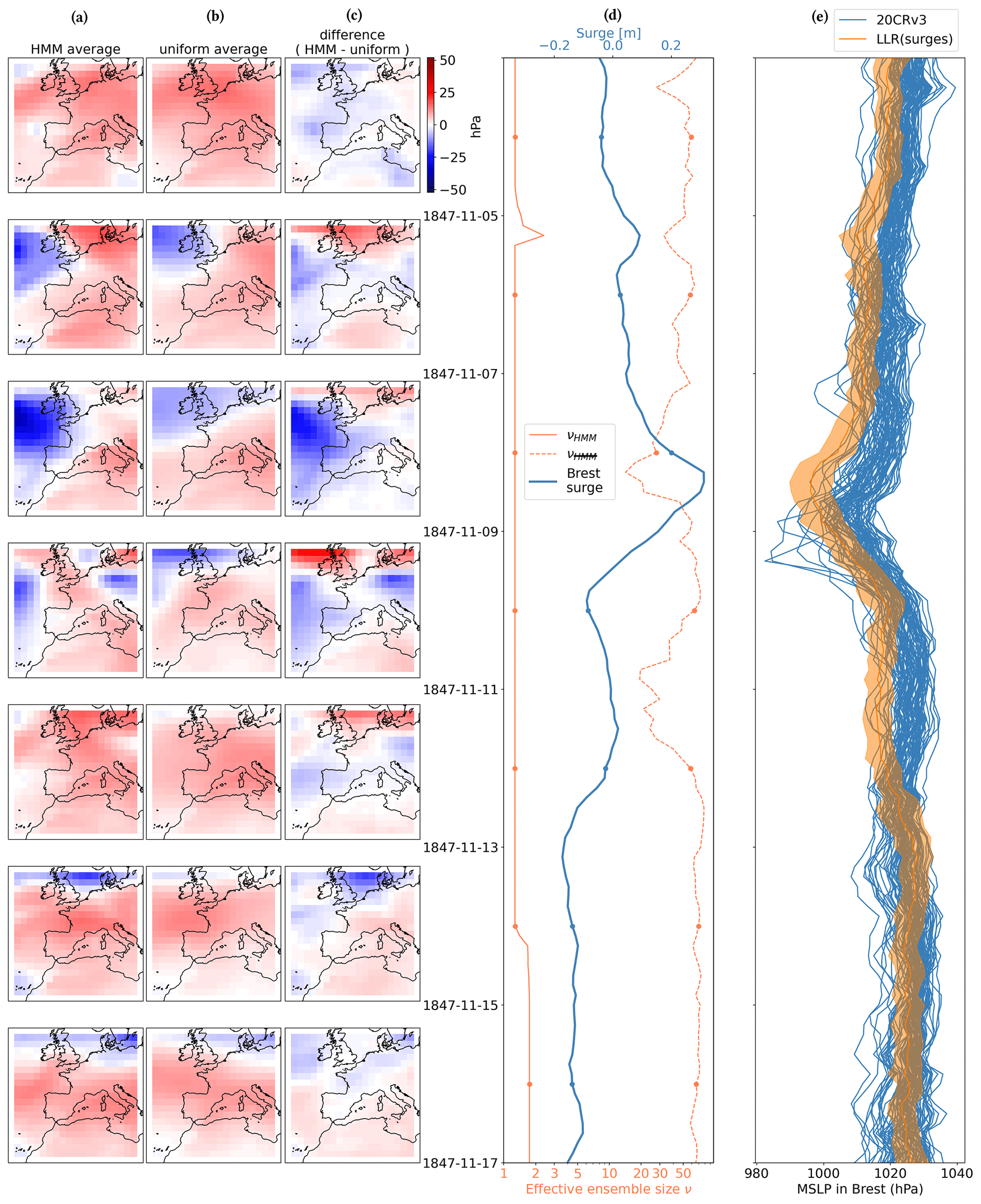
Figure 10 Mean result of the HMM algorithm in November 1847. (a) Average according to surge residual observations and HMM smoothing algorithm (probabilities p_HMM(i,t)). (b) Average using constant uniform weights on 20CRv3 members. (c) Difference between HMM and uniform results. (d) Surge residual observations and effective ensemble sizes. (e) MSLP in Brest from ensemble members (blue lines) and local linear regression from surge residuals as an average ±1 SD (standard deviation). The dates of the left-hand plots are indicated with dots in (d) and (e).

Figure 11 The same as Fig. 10 but for another storm. In this figure independent pressure observations in Brest are also available and shown as black dots in (e).

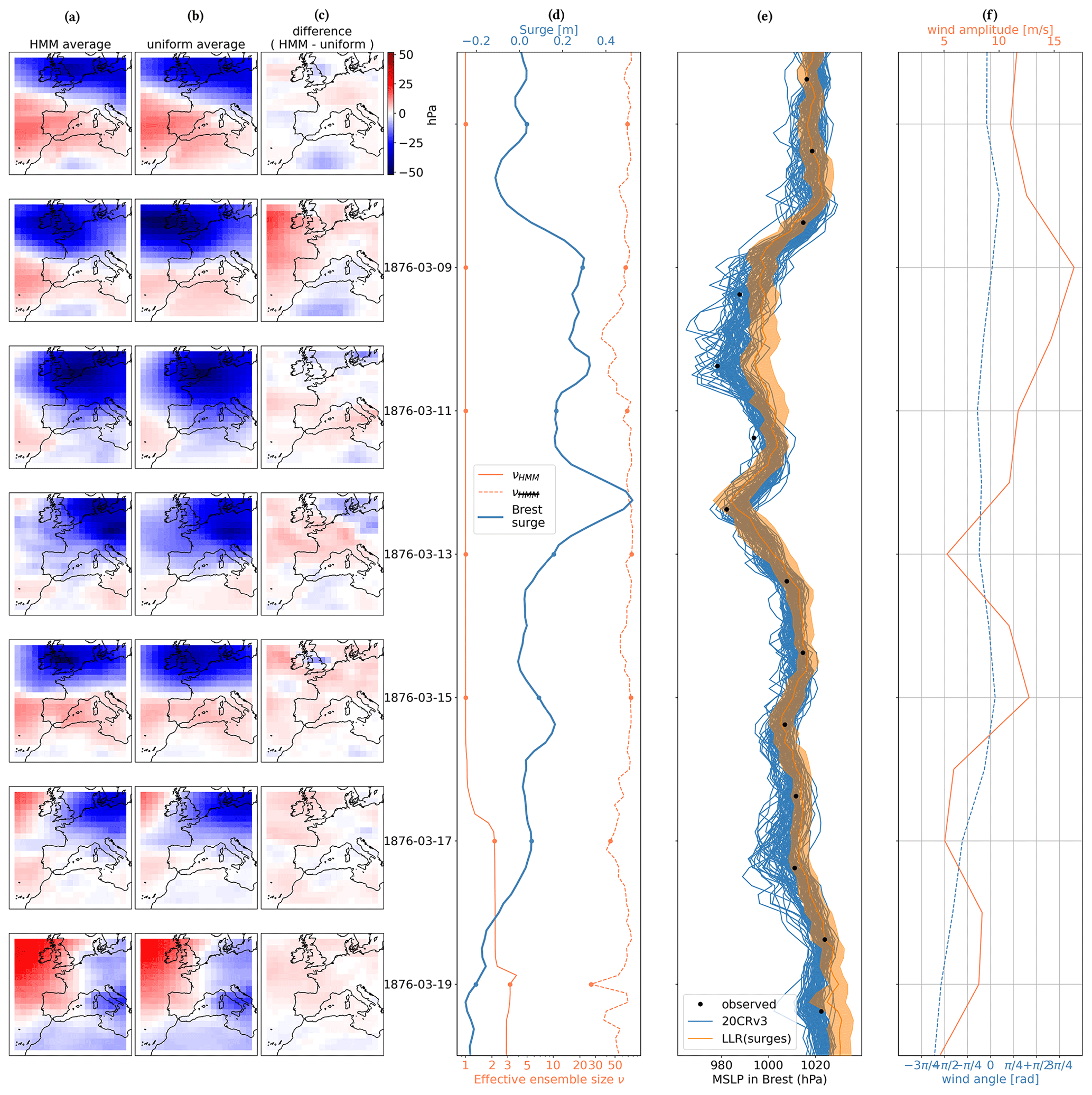
Figure 12 The same as Fig. 11 but for another storm. In (f) we also show the amplitude and direction of daily 10 m winds from the 20CRv3 member mean linearly interpolated at the city of Brest.

Figure 13 The same as Fig. 11 but for another event.

One common feature of Fig. 10–12 is that the HMM algorithm tends to be very selective compared to the weighing without HMM. This is the consequence of our optimization of the parameter θ with the objective of maximizing the likelihood of the surge residual observations on the 20CRv3 ensemble. Having a low theta value allows us to give a high weight to the ensemble member that has the highest probability according to the surge-residual-based LLR model. However, as is obvious from comparing Fig. 10a with b, Fig. 11a with b, and Fig. 12a with b, this does not always have a strong influence on the average MSLP field. In the case of Fig. 13, the variability between members of the reanalysis is smaller, and therefore the selection of ensemble members is less acute, with more reasonable effective ensemble sizes. However, these figures again show that small effective ensemble sizes should not be interpreted as a justification for discarding members with low probability according to the HMM algorithm but rather as a means to quantify the relative agreement of individual members with the surge residual observations according to the LLR statistical relationship.

The fact that one member is often much more coherent with the series of surge residuals is the result of (1) the high variability of the ensemble and the LLR pressure estimation, (2) the high dimensionality (or complexity) of the problem, (3) the low size of the ensemble (80 members), and finally (4) the systematic biases between 20CRv3 and the LLR caused by unmodeled atmospheric conditions (winds). Indeed, in the case of data scarcity, the variability of the reanalysis is large (point 1), and a fixed-size ensemble (point 2) may struggle to correctly span the whole space of possible atmospheric circulations (point 3), meaning that a few members are actually much closer to the true atmospheric circulation than all other members. Such a problem is called filter degeneracy (Snyder et al., 2008) and is a common issue in ensemble-based data assimilation schemes. Secondly, since our LLR estimation of pressure experiences time-correlated biases with respect to the 20CRv3 because of unmodeled other variables (winds), this causes the HMM to select the one member that is closest to the biased pressure estimate from the LLR applied to the surge residual signal. All these issues may remain for other climate science applications if one uses a similar approach of merging independent observations with a HMM algorithm to weight ensemble members.

6 Conclusion and perspectives

This study is a proof of concept for the use of century-old tide gauge data as a means of understanding past atmospheric subseasonal variability. Surge residuals of Brest allow us to assess part of the atmospheric variability that was uncaught in global 20CR reanalyses based on pressure observations. Weighing 20CR members according to surge residual observations reduces the effective ensemble size and implies significant deviations in member-averaged sea level pressure in the Bay of Biscay. Through the second half of the 19th century these deviations diminish and the effective ensemble size rises; however, they remain non-negligible. Independent pressure observations in the city of Brest are coherent with pressure estimations from the reanalysis and the surge-residual-based local linear relationship. Such comparisons also show that the reconstruction of pressure based on surge residuals is ambiguous due to the influence of winds, meaning that biases between the surge-residual-based and reanalysis-based pressure estimates can last for several days.

This work has several potential applications. First, replicating this work with other tide gauges could help us to validate reanalyses like 20CRv3 against independent data and to potentially identify anomalous trends or incorrect estimations of specific events. Combining our statistical approach with the physics-based approach of Hawkins et al. (2023) could allow us to have both a precise estimate from a high-fidelity coastal model and a good quantification of uncertainties. Second, tide gauges could be used to constrain regional-scale atmospheric simulations in order to better estimate the magnitude and spatial extent of known past severe storms. Third, tide gauge records could be combined with direct observations of atmospheric pressure to give statistical estimates of atmospheric fluctuations in the 19th century without the use of an NWP model, such as the optimal interpolation of Ansell et al. (2006) based on direct pressure observations only or the analogue upscaling of Yiou et al. (2014) for the short period 1781–1785 of dense observations in western Europe. Finally, this work could be replicated in a more general context using other types of variables and observations, learning the relationship between observations and large-scale features using recent observations and precise reanalyses, and applying these statistical relationship in the past to uncover past large-scale events. In particular, the hidden Markov model algorithm outlined here could be replicated to weigh ensemble members according to independent observations.