The weather of 1740, the coldest year in central Europe in 600 years

The winter of 1739/40 is known as one of the coldest winters in Europe since early instrumental measurements began. Many contemporary sources discuss the cold waves and compare the winter to that of 1708/09. It is less well known that the year 1740 remained cold until August and was again cold in October and that negative temperature anomalies were also found over Eurasia and North America. The 1739/40 cold season over northern mid-latitude land areas was perhaps the coldest in 300 years, and 1740 was the coldest year in central Europe in 600 years. New monthly global climate reconstructions allow us to address this momentous event in greater detail, while daily observations and weather reconstructions give insight into the synoptic situations. Over Europe, we find that the event was initiated by a strong Scandinavian blocking in early January, allowing the advection of continental cold air. From February until June, high pressure dominated over Ireland, arguably associated with frequent eastern Atlantic blocking. This led to cold-air advection from the cold northern North Atlantic. During the summer, cyclonic weather dominated over central Europe, associated with cold and wet air from the Atlantic. The possible role of oceanic influences (El Niño) and external forcings (eruption of Mount Tarumae in 1739) are discussed. While a possible El Niño event might have contributed to the winter cold spells, the eastern Atlantic blocking is arguably unrelated to either El Niño or the volcanic eruption. All in all, the cold year of 1740 marks one of the strongest, arguably unforced excursions in European temperature.

1 Introduction

The winter of 1739/40 is known as an extremely cold winter in central Europe, rivalling the winter of 1708/09 as the coldest in the past several hundred years. The winter was severe across Europe, including Switzerland (Pfister and Wanner, 2021), Poland (Filipiak et al., 2019), the British Isles (Manley, 1957; Lamb 1967, Jones and Briffa, 2006), the Netherlands, Germany, and other regions. The winter started early, already in October 1739, and ended only in June 1740, and it is particularly well known for frozen rivers and ice floods. In London, a frost fair was held on the River Thames, and in Ireland the River Shannon froze (Dickson, 1997; see Mateus (2021) for an overview of early instrumental data in Ireland). In Italy the lagoon of Venice froze (Camuffo, 1987). Filipiak et al. (2019) reported that, after unusually cold easterly winds in mid-October 1739 on the coast of the Baltic Sea, there were very heavy snowfalls and several waves of severe frost in November 1739 and January 1740 and again in February and March, with the most extreme conditions in January 1740. The coastal waters of the Baltic Sea and particularly the Vistula River were frozen until mid-April, with the ice thickness exceeding 50 cm. Water from the huge amounts of snow melting in April caused a large and long-lasting flood in the Baltic lowlands. In Ireland, the intense cold lasted for weeks, interspersed with only a short break and a slight thaw (Gillespie, 1939). Potatoes and turnips were destroyed, and cattle and even fish died (Dickson, 1997). Among the consequences was the Irish famine of 1740/41 (Engler et al., 2013), triggering substantial migration. However, the winter was only the start of a series of adverse weather and climate events, which also led to high mortality and high cereal prices in central Europe (Post, 1984). Due to the frozen rivers and long-term shutdown of mills in Poland, there was even a shortage of bread, and the administrative authorities of many cities started to provide food, wood, and means of subsidence to the poorest people (Filipiak et al., 2019). Jones and Briffa (2006) pointed out that the entire year of 1740 was cold and that it particularly contrasted with the warm 1730s. The annual average Central England Temperature was above the 1961–1990 average in all years from 1730 to 1738 (Manley, 1974; Parker et al., 1992).

Reconstructions of sea-level pressure have allowed us to characterize the anomalies in atmospheric circulation of this specific period in a bit more detail. Jones and Briffa (2006), using hand-analysed monthly sea-level pressure fields, noted that, in winter, the Icelandic Low and the Azores High were weaker than normal and that the dominant feature was a continental or Scandinavian high. Engler et al. (2013), using sea-level pressure and the 500 hPa geopotential height reconstruction of Luterbacher et al., (2002), additionally found a strong high-pressure situation in spring 1740, resembling a negative phase of the East Atlantic (EA) pattern and leading to cold-air advection from the northwest.

It is less well known, however, that the winter of 1739/40 was not only cold in Europe but also in North America and parts of Asia. A cold-season (October–May) temperature field reconstruction for mid-latitude (35–70° N) land areas from 1701–2020 indicates that this might have been the coldest cold season of the last 300 years (Reichen et al., 2022). Recently, a comprehensive global three-dimensional climate reconstruction was published (Valler et al., 2024), and numerous additional meteorological time series have been digitized such that we can now study this event in more detail and on a daily scale, i.e. the scale of the weather events.

Here we study the weather of the year of 1740 using the new reconstructions combined with daily meteorological series. We analyse the sequence of events on a monthly scale, zoom into prominent cold-air outbreaks on a daily scale, and analyse the role of forcings and large-scale circulation mechanisms.

2 Data and methods

Reconstructions

We use the Modern Era Reanalysis (ModE-RA) family of reconstructions (Valler et al., 2024), which provide monthly global three-dimensional fields back to 1421. Similarly to the precursor product EKF400v2 (Valler et al., 2022), ModE-RA is based on the offline assimilation of a large number of natural proxies, documentary data, and instrumental observations into an ensemble of 20 atmospheric model simulations (ModE-Sim; Hand et al., 2023). Another product, termed ModE-RAclim, was generated by assimilating the same observations into a sample of 100 realizations, randomly drawn from all members and all model years of ModE-Sim. Analysing ModE-Sim and ModE-RAclim along with ModE-RA allows us to disentangle the role of forcings and observations. ModE-Sim was forced by monthly sea-surface temperatures (Samakinwa et al., 2021; Titchner and Rayner, 2014) and by volcanic, land-surface, and solar forcings following the PMIP4 protocol (Jungclaus et al., 2017). It does not see the assimilated observations, but it only sees the model boundary conditions. In contrast, ModE-RAclim does not see the time-dependent boundary conditions, but it only sees the observations. We performed the analyses on the individual ensemble members, but when plotting spatial fields we show the ensemble mean only. When plotting anomalies, these were expressed relative to the 30 preceding years (1710–39). Note that the ModE-RA data set was constructed as a set of anomalies from a 71-year moving average; therefore the last 3 decades of the data set are less well constrained.

For comparison, we also used the reconstruction XBRW_CCC (Reichen et al., 2022), which provides cold-season (October–May) temperature field reconstructions for the northern extratropics. It is based on a Bayesian reweighting approach of model simulations that are very similar to ModE-Sim. Only phenological data (mostly ice phenology, i.e. the freezing and thawing dates of rivers and lakes, and some plant phenological data) are used to constrain this reconstruction.

Table 1 Locations and sources of daily weather data used in this study, along with variables (Var.; p is pressure, mslp is mean sea-level pressure (converted by other authors), T is temperature, dir is wind direction, RR is precipitation, and wn is weather notes), period, and source.

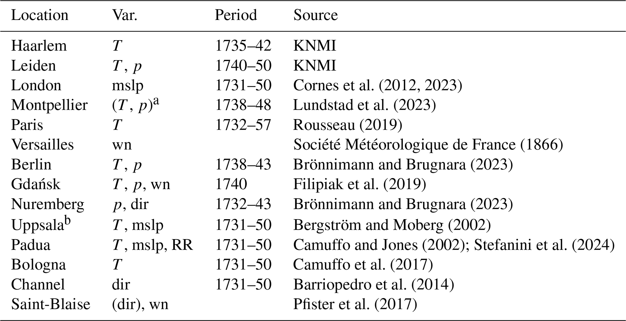
^a Pressure was only used until April 1746, and morning (typically 3–8 AM) and afternoon (mostly 3 PM) were treated separately. ^b Until 1738, these were presumably indoor measurements (Bergström and Moberg, 2002), which have a reduced diurnal cycle amplitude and perhaps also day-to-day variability but only a small bias.

Meteorological series

In this paper we work with daily meteorological time series from measurements and observations, which were inventoried in Brönnimann et al. (2019) and compiled in Lundstad et al. (2023). These compilations are complemented with additional series. Table 1 gives an overview of the series used and their sources. Note that there are several additional sources that only provide monthly data. They are not listed in the Table but are included in the ModE-RA data set. Prominent long monthly temperatures are those from De Bilt, the Netherlands, since 1706 or from the Central England Temperature since 1659 (but daily only after 1772; Parker et al., 1992).

For some of the analyses, all segments were deseasonalized by fitting and subtracting the first two harmonics of the annual cycle and then standardized. This allows a better comparison of series with different numbers of observations per day and allows us to include series on unknown scales (such as temperature in Berlin). Note that a unique reference period that works for all series does not exist. If possible, we used 1731–50, but several of the segments were too short (in one case slightly longer, following an existing segment). This reference is shorter than that for ModE-RA (analyses of the two data sets are performed separately). For the special case of Montpellier, where we have very irregular data (but which always include the monthly minima and maxima), we proceeded in the same way for the deseasonalizing. However, because the series consists mostly of maxima and minima, it has a standard deviation that is ca. 1.5–2 times larger than that at other stations. Therefore, we inflated the standardized anomalies by 1.5.

In addition to the instrumental series, we also consulted weather diaries and other historical sources to better characterize the weather of 1740. This includes observations from Gdańsk (Filipiak et al., 2019), Berlin (Brönnimann and Brugnara, 2023), Versailles (Société Météorologique de France, 1866), and Saint-Blaise (from Euro-Climhist; Pfister et al., 2017). Note that most of these series were assimilated into ModE-RA.

Daily reconstructions of sea-level pressure fields

For the analyses of daily weather, we not only used the raw data, but we also reconstructed daily pressure fields over Europe from the pressure observations using a simple analogue approach (see also Pappert et al., 2022). For that, we used the ERA5 reanalysis (Hersbach et al., 2020) from 1940–2023. We extracted sea-level pressure at the 1740 observation locations, deseasonalized and standardized the data in the same way as described above (using the entire period), and then determined, for each day in 1740, the closest analogue day in ERA5 within a window of ± 60 calendar days of the target day. We used the Euclidian distance as a distance measure. Once the closest analogue was found, the sea-level pressure field for that day was taken as the reconstruction, without any further postprocessing.

An evaluation was performed by applying the procedure to the year 1940 within ERA5 using 1941–2023 as a pool of analogues. Comparing the results with the actual fields in 1940 (Fig. S1 in the Supplement) shows excellent correlations and a low root-mean-square error over central Europe but a rapid deterioration towards the southwest and northeast.

Index time series

In addition to spatial analyses and analyses of the instrumental series, we also calculated time series within ModE-RA. We defined central European temperature as the average 2 m temperature in the region 45–55° N, 5–25° E. The index was also calculated in the CRUTEM5 data set (Osborn et al., 2021) in order to extend the reconstruction to the present. Furthermore, we calculated indices for the North Atlantic Oscillation (NAO), the Scandinavia Index (SCAN), and the East Atlantic (EA) pattern. NAO was defined as the sea-level pressure difference between the locations of Lisbon and Gibraltar. SCAN was defined as the sea-level pressure difference between 40° N, 15° E and 65° N, 30° E. For the EA pattern, different definitions exist. We used the sea-level pressure difference between 45° N, 30° E and 55° N, 20° W, which is similar to Barnston and Livezey (1987) and which we denoted as EA1 in the text. We also defined an index EA2 as the difference between 55° N, 30° E and 55° N, 20° W, which is more similar to the definition of Wallace and Gutzler (1981). Note that, in all indices, only the difference was calculated and no standardization was used, since the standard deviation in the ModE-RA data sets changes over time. We mostly analysed January–February for NAO and March–May for EA1 and EA2.

Figure 1 Excerpt from the “Kirch diary” written by Christine Kirch for 13 and 14 January 1740 (see Brönnimann and Brugnara, 2023).

Finally, we also used a Niño 3.4 index (September–February), which we calculated from ModE-RA 2 m temperature data. For addressing the volcanic forcing, we used the estimated radiative forcings for different volcanic eruptions as given in Sigl et al. (2015). We selected eruptions with a global forcing stronger than −2 W m⁻². For both Niño 3.4 and volcanic years, we analysed the NAO and EA indices of the subsequent winter and spring. For Niño 3.4 we used a correlation analyses, and for volcanic eruptions we used compositing.

3 Results

Descriptions of the weather and impacts in Europe

The low temperatures in the winter of 1739/40 and the consequences thereof are well documented across Europe. Here we present the weather information from the three locations listed in Table 1 (Versailles, Gdańsk, and Saint-Blaise). Interestingly, the winter of 1739/40 was compared with the winter of 1708/09, which was still in living memory at that time, in several sources. As an example, Fig. 1 shows an excerpt of a weather diary written by Christine Kirch (Brönnimann and Brugnara, 2023). The text, describing a travel from Paris to Luxembourg, speaks of freezing wine, fountains freezing to the ground, and bursting bridges. In several instances it compares measured temperatures with those in 1709 and finds that 1740 temperatures were even lower.

Commissaire Narbonne noted the weather in Versailles from 1709–45 (Société Météorologique de France, 1866). According to his notes, the Seine was frozen, and public fires were lit in the streets of Paris from 9 January to 9 February 1740 and similarly in Versailles. Severe frost is noted in January, February, and March. Low temperatures are noted throughout the year. On 7–8 October, during grape harvest, Versailles experienced a severe frost and grapes were frozen.

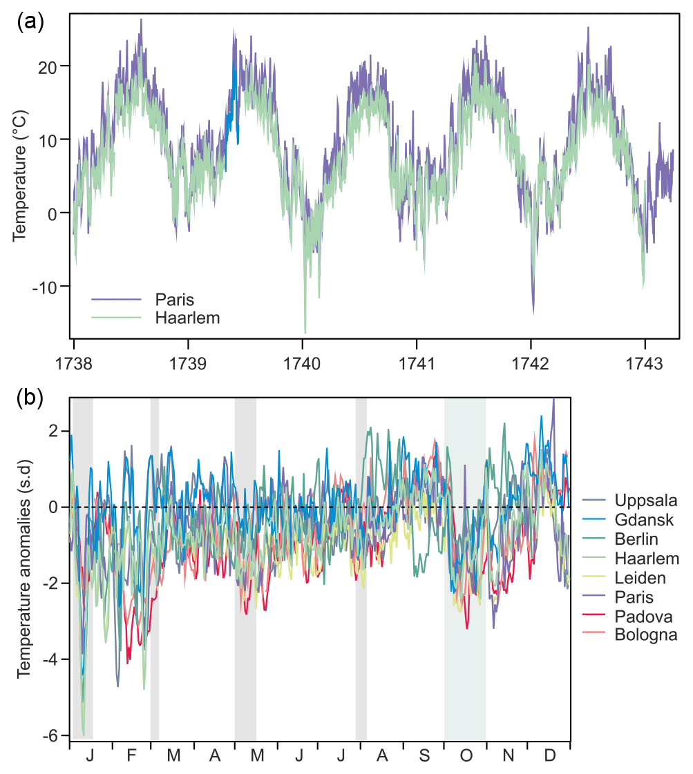
Figure 2 (a) Daily temperature series from two selected European stations from 1738–43 and (b) the standardized daily temperature anomaly at seven European sites in 1740. Shaded bars in the middle panel denote the periods chosen for more detailed analysis.

According to two prominent scientists of Gdańsk on the Baltic Sea coast, northern Poland, Michael Christian Hanov (a pioneer of systematic instrumental measurements in the city) and Gottfried Reyger (botanist and chronicler), the winter of 1740 in Gdańsk was unprecedented (Filipiak et al., 2019). Hanov recorded the lowest temperatures between 8 and 14 January 1740 with a minimum on the morning of 10 January. Furthermore, extreme cold also occurred between 1 and 7 February, 17 and 25 February, and in a few selected days in March. Reyger compared several severe winters in the 18th century (1709, 1729, 1740, and 1784) and pointed out that winter of 1740 was undoubtedly the coldest one; however, in 1709, the duration of severe frost was even higher. Harsh weather conditions during winter and a late and cool spring resulted in a very late appearance of vegetation – species usually present in early March were observed only in the last days of April. Although the ice on the Baltic Sea and the Vistula remained for a longer time in April 1771 and 1784 than in 1740, the flood lasting many weeks had a significant impact on the economy in 1740. Both researchers noticed unnatural behaviour in animals and numerous cases of animals freezing, both farm animals and wild ones. Among the increased number of human diseases, many cases of frostbite were noticed, but the mortality rate did not increase noticeably. Furthermore, Hanov pointed out an exceptionally cold May with extremely cloudy conditions (whereas cloudiness is usually minimal in May), fog and snow constantly present even at the end of the month, several frosts in June, and unusual weather conditions during summer. The harvest, delayed by a cold and wet August, took place in an exceptionally sunny and warm September (according to Reyger it was “the best weather in the whole year”), and the autumn fruit harvest was also very good. October was cold again in Gdańsk. The first snowfall already occurred on 5 October. Hanov also reported the anomalously cold weather in selected months of 1740 (particularly in January) in other cities in Europe, e.g. Kaliningrad, Hamburg, Kiel, Wittenberg, the Hague, Uppsala, and Saint Petersburg.

In Switzerland, a detailed weather diary is available from the vine-grower family Péter from Saint-Blaise. The diary notes the very low temperatures from 8–12 January, which were followed by warmer weather. However, all of February was then described as “very cold” in Saint-Blaise. In February and March, water bodies were frozen and navigation stopped on Lake Biel and Lake Morat, and this continued into April (on 19 April, parts of Lake Neuchâtel were frozen). For most of March, the weather diary notes “frost”. Frost impact on grapevines was reported in April and May. Snowfall was observed until 8 May (at low elevations) and 20 May (at higher elevations).

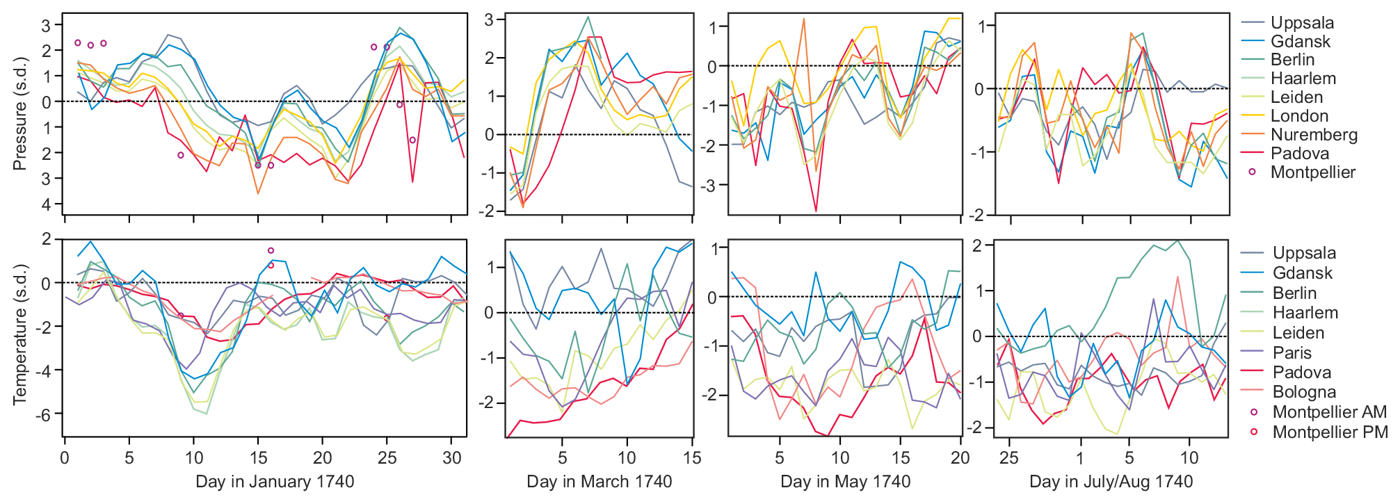
Figure 3 Standardized temperature and sea-level pressure anomaly series for the four episodes of 1–31 January, 1–15 March, 1–20 May, and 24 July–14 August 1740.

Instrumental measurements

For the year 1740, eight daily temperature series are available, although Montpellier is very sporadic and Haarlem and Leiden are very close. More series would exist, but they are not available in daily, digitized format (see Brönnimann et al., 2019). As an example, Fig. 2a shows the raw daily mean temperature series from Paris and Haarlem from 1738–43. The low temperatures in the winter of 1739/40 clearly stand out, and it becomes visually apparent that the other seasons were also colder than in the other years shown (the winter of 1741/42 is also very cold). The winter of 1739/40 began early, with low temperatures in October and November 1739. After a warm December, temperatures then dropped in January. Low temperatures lasted consistently until August, and October and November were again very cold.

Figure 4 Standardized anomalies of pressure and temperature, along with weather observations at stations and analogue sea-level pressure reconstruction (hPa) for four selected periods in January, March, May, and July/August 1740.

After deseasonalizing and standardizing the series (Fig. 2b), it can be seen that temperatures were below average (1731–1750, where possible) at most stations during most of the year. Only August and September had warm intervals. In this work, we discuss several episodes (marked with grey bars) in more detail by analysing the daily series (Fig. 3) and pressure fields (Fig. 4).

One of the most severe cold spells occurred in the first half of January 1740. It peaked on 10–11 January and brought very low temperatures to western Europe, up to 6 standard deviations below the mean, which is extraordinary (Fig. 3). The cold was not so intense in the north and south, i.e. in Uppsala and Bologna (although temperature also fell below −2 standard deviations at those locations; note that, in Uppsala, part of the reference period is based on indoor data). Temperatures also remained low during the rest of the month, with a similar pattern. Pressure was below normal in the south and above normal in the north; the gradient in the standardized anomalies persisted during the entire month. The distinct pressure drop in Padua on 27 January is suspicious and could be an outlier, but Montpellier also shows a pressure drop.

In early March 1740, negative temperature anomalies were observed in the south and west, though not nearly as strong as in January. All stations show a very strong pressure increase from strong negative anomalies to very high positive anomalies that persisted for 10 d. The third cold period, in May 1740, was less homogeneous. Again, temperatures were persistently low in western Europe (Paris and Leiden) and only slightly below normal in Gdańsk and Uppsala. Temperatures were also low in Bologna at the beginning of the month and again towards 20 May. Pressure was generally below normal, but it was above normal in London.

The fourth chosen episode featured below-normal temperatures at most stations. An exception is Berlin, where temperatures exceeded 2 standard deviations. This appears suspicious, but we have no indications that could lead us to remove the data. Pressure was mostly below normal. Padua and Uppsala sometimes show different behaviour, whereas all other stations run in parallel. Overall, analysing the long pressure time series from London or Uppsala, the year 1740 did not feature particularly many extreme days.

Weather maps

Plotting the daily data on a map, along with the weather observations and the analogue pressure reconstructions, allows an inspection of the pressure systems and of the flow over central Europe. During the cold spell in January (Fig. 4, top), a strong high-pressure system established over Scandinavia, and at the same time a rather strong low-pressure system developed over the northern Mediterranean, causing a strong inverse pressure gradient across Europe. This situation can firmly be addressed as a Scandinavian blocking event, allowing cold continental air to flow in from the east. The main spell lasted only 5 d, but further similarly extreme cold spells occurred in January and February. In the latter cases, positive pressure anomalies were strongest over London but stretched into Scandinavia (not shown). Note that the sea-level pressure maps are based only on pressure observations and are independent of temperature and wind observations.

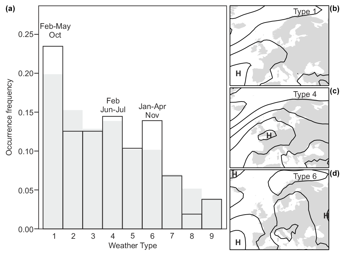
Figure 5 Frequency of daily weather types in the CAP9 classification in 1740 (open rectangles) and in the period 1991–2020 (grey). Right insets show the composite fields for sea-level pressure for types 1, 4, and 6, respectively, in 1940–2020 from ERA5.

In the first half of March, pressure was high everywhere and temperatures were below normal everywhere except in Uppsala. Figure 4 depicts the beginning of this high-pressure period. After a strong low-pressure situation, pressure began to build up in the west (UK) and then established over the continent. The strongest pressure anomalies were observed first in Gdańsk and Berlin. Again, continental Europe was in an easterly flow, bringing relatively (though not extremely) cold continental air to central and western Europe.

The generally low temperatures in 1740 not only included sharp but temporally limited drops in temperature due to cold spells, but also longer, persistent phases of below-normal temperature. An example is the third selected period in May 1740. During this period, pressure was relatively low over continental Europe and arguably higher over England. The monthly mean reconstruction shows a strong East Atlantic pattern throughout spring. Frequent westerly or northwesterly wind arguably brought cold air from the northern North Atlantic, which at that time of the year is very cold relative to the land. Finally, the lowest row in Fig. 4 shows a situation in late July and early August. It was rather cold and rainy, with typical cyclonic weather dominating. The fifth period noted in Fig. 2 is the month of October, which was persistently cold at most stations. For reasons of length, the period is analysed in this work based on monthly charts rather than daily.

Before focusing on monthly charts, though, we would like to analyse how the daily sea-level pressure maps translate into monthly means. For this we analysed the frequency of daily weather types over central Europe, specifically the Cluster Analysis of Principal Components with 9 types (CAP9) classification that reaches back to 1728 (Pfister et al., 2024). Three weather types were overrepresented in that year, namely 1, 6, and, to a lesser, extent 4. These patterns (displayed in Fig. 5, right) are mostly types with high-pressure systems over western Europe.

Figure 6 Monthly anomalies (with respect to 1710–39) of (a) temperature and (b) sea-level pressure in 1740 in the ModE-RA ensemble mean. The bottom figure also shows sea-level pressure anomalies from the analogue approach (relative to 1991–2020, contour distance 2 hPa centred around zero, negative dashed).

We now turn to the analysis of monthly anomaly fields in the ModE-RA data sets (Fig. 6; see Fig. S2 in the Supplement for monthly anomaly fields from October–December 1739) and specifically the fields for October. Temperature anomalies in this month were negative in central Europe. Although they were not as strong as during the winter months January to March, they reached down to −4 °C, which is remarkable for this time of the year. As noted earlier, severe frost was observed in Versailles such that the grapes froze.

In ModE-RA we can also analyse monthly anomaly fields of sea-level pressure (Fig. 6b; fields for October–December 1739 are shown in Fig. S2). From January to June and then again in October and November, we find positive sea-level pressure anomalies in the eastern Atlantic and negative ones over Eastern Europe. This is similar to the East Atlantic pattern, which we will address later. The positive anomalies could point to more frequent blocking situations. In Fig. 4 (top), we address Scandinavian blocking for the cold spell in January. However, this is not seen in the monthly average, where the core of the positive anomaly is situated further to the west. The pattern more resembles a negative North Atlantic Oscillation index, although the anomaly centres are shifted southeastward.

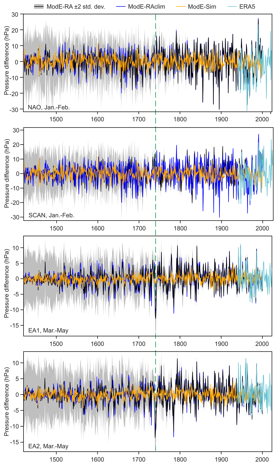
Figure 7 Indices of the NAO and SCAN in January–February and of the EA1 and EA2 in March–May relative to 1710–39. Shown are the three data sets ModE-RA (grey shading denotes ± 2 standard deviations of the ensemble), ModE-RAclim, and ModE-Sim, as well as ERA5. The dashed green line marks the year 1740.

Figure 8 Annual mean anomalies of (a–c) temperature and (d–f) sea-level pressure in 1740 in (a, d) ModE-RA, (b, e) ModE-RAclim, and (c, f) ModE-Sim. Also shown are the location and types of observations for October 1739–March 1740 on which ModE-RA and ModE-RAclim are based. The yellow rectangle (a) shows the region defined as central Europe. Panel (f) shows the definition of NAO, EA and SCAN indices.

We calculated indices for the NAO and SCAN for January and February and for the East Atlantic pattern for March to May for all three ModE products (Fig. 7; the ensemble spread is only shown for the ModE-RA for better visualization). In ModE-RA and ModE-RAclim, which are very similar, the NAO was negative in 1740, but it was by no means an extreme year. Likewise, the SCAN index is negative but not extreme. However, the negative East Atlantic pattern in spring is unique in the entire record since 1421, both for EA1 and EA2 (very similar results are found in the annual mean). The analysis of ModE-Sim shows that only a small part of the variability is reproduced purely from the model boundary conditions, which means that presumably the forced component of the signal is relatively small, at least in ModE-Sim. In order to extend the series to the present, we also calculated the indices in ERA5 (using 1991–2020 as a reference, correlations in the overlapping period for NAO, EA1, and EA2 are 0.992, 0.936, and 0.949, respectively). Neither of the series shows a trend, neither in ModE-RA nor in ERA5. Also, no clear change in variability is seen in ModE-RA, although the recent variability in the NAO in ERA5 is very large in a 600-year context.

An interesting aspect of the monthly analysis is the persistence even at a seasonal and longer timescale. In particular, the East Atlantic pattern is persistent or recurring. We therefore also analysed the annual mean fields of temperature and pressure anomalies (Fig. 8). Again, ModE-RA and ModE-RAclim show very similar patterns. For temperature, the ModE-Sim shows negative temperature anomalies of up to 0.5 °C over parts of Europe; hence there is a contribution of boundary conditions on a large scale, though much weaker than the full reconstruction. For sea-level pressure, there is no contribution from ModE-Sim. The pattern in the annual mean sea-level pressure anomaly is more similar to the East Atlantic pattern of Wallace and Gutzler (1981) rather than the corresponding pattern in Barnston and Livezey (1987).

Figure 9 (a) Time series of cold-season (October–May) mean temperature over northern extratropical (35–70° N) land areas (XBRW_CCC). (b) Time series of annual mean central European temperature in three reconstructions: ModE-RA, ModE-RAclim, and ModE-Sim. Shadings indicate 2 standard deviations of the ensemble.

To analyse how cold the year 1740 really was, we calculated central European mean temperature in the three data sets. In fact, in ModE-RA, 1740 is the coldest year on record back to 1421 (outside the lower confidence interval of ModE-RA of any year), followed by 1829/30 (Fig. 9). The coldest 12-month period (not shown) is November 1739 to October 1740. The annual mean temperature of 1740 was 2.15 °C below the preindustrial mean (1851–1900). Also shown are CRUTEM5 data in order to extend the climate reconstructions into the present. These data show a warming of 2.5 °C since the preindustrial, such that the cold year 1740 was more than 4 °C cooler than the present.

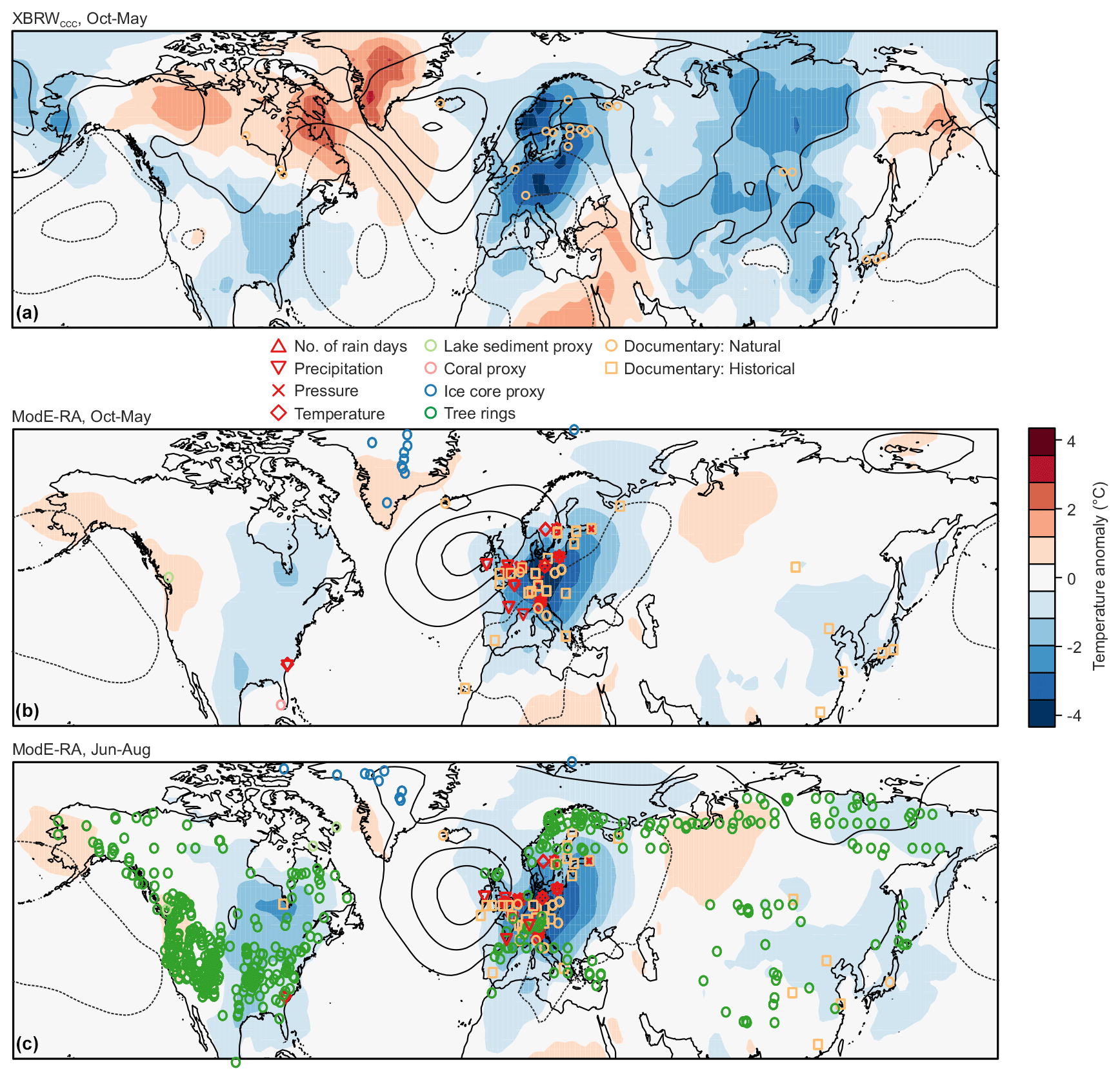
Figure 10 Anomalies of temperature and sea-level pressure (contour distance 2 hPa centred around zero, negative dashed) for (a) the cold season (October–May) of 1739/40 in the XBRW_CCC data set (Reichen et al., 2022), (b) the cold season of 1739/40 in ModE-RA, and (c) summer (June–August) in ModE-RA, expressed as anomalies from the preceding 30 years. For XBRW_CCC, which is based only on phenological data, orange circles mark the locations (displayed with a slight offset if several observations, e.g. freezing and thawing dates, are available from the same location). For ModE-RA, observations entering the data set are also shown.

A large-scale view

The winter of 1739/40 was not only cold in Europe, but also over North America and Eurasia. This can be seen in a recent reconstruction of cold-season (October–May) temperature based only on phenological data (Fig. 10). In fact, 1739/40 was the coldest cold season in the land-area-averaged temperature between 35 and 70° N in this reconstruction (which reaches back to 1701; Reichen et al., 2022; see Fig. 9a). The low temperatures in North America are confirmed by a temperature series from Charleston (Fig. S3 in the Supplement) that was not included in the reconstruction shown in Fig. 10. In fact, this is also confirmed with documentary data. In North America, the summer of 1740 was cool and wet (Perley, 1891). However, in ModE-RA, Siberia is warmer than in XBRW_CCC.

Documentary data from China show that spring 1740 was late, both in northern China and in southern China, with the end date of snow being around 20 d later than average in the Beijing–Zhangjiakou region and Nanjing (Gong et al., 1983). However, although narrative evidence shows that the winter, especially the late winter, may have been colder than average in southern China (Ding and Zheng, 2017; Zhang, 2013), it was not an extremely cold winter based on existing reconstructions of eastern Asia (Hao et al., 2018; Wang et al., 2023).

The summer (June–August) temperature anomaly fields are very similar to those of the cold season (Fig. 10). One reason might be that, for some of the rivers, the thawing takes place only shortly after the start of the warm-season assimilation window and these proxies are assimilated for both the cold and warm season. Likewise, since the warm-season assimilation window covers April–September, the tree ring proxies in ModE-RA also affect the October–May period. However, the persistence might also be real, as it also appears in the analogue reconstructions (contours in Fig. 6). Similarly to the cold season, Siberia has also positive temperature anomalies in summer (arguably due to tree rings) such that the annual mean of 1740 was not the coldest year on record in global mean temperature in ModE-RA. Sea-level pressure anomalies show the clear EA pattern over Europe. In addition, they show a positive phase of the Pacific–North American (PNA) pattern, most pronounced in XBRW_CCC.

Role of forcings

Finally, we analysed the role of oceanic influences (i.e. Niño 3.4 in our case) and of external forcing due to volcanic eruptions. ModE-RA, which is based on the monthly sea-surface temperature reconstructions by Samakinwa et al. (2021), which in turn are based on annual reconstructions by Neukom et al. (2019), show El Niño conditions in 1739 and partly in 1740. To analyse the possible role of El Niño, we performed a correlation analysis, restricting our analysis to the years 1710–2000 because of the deteriorating quality further back. Results (Fig. S4 in the Supplement) show that almost all correlations for all ensemble members for all indices (NAO in January–February and EA1 and EA2 in March–May) are within ± 0.1. The strongest (negative) correlations are found for the NAO. The box plots show the spread among the ensemble members, which should not be confounded with the significance of the correlations themselves. In fact, none of the correlations are statistically significant at p = 0.05.

Another influence could have come from the volcanic eruption of Mount Tarumae, 19–31 August 1739. In the volcanic forcing data sets used in ModE-RA and in Sigl et al. (2015), this is not a very big eruption, but, with a global forcing of −2.4 W m⁻², it exceeds the threshold set in the Data and methods section. We analysed all eruptions with a global forcing stronger than −2 W m⁻², again restricting ourselves to the time period 1710–2000 (Fig. S3). We find only weak effects of strong eruptions on circulation, such as a slightly positive response of the NAO in January–February and positive responses of the EA1 and EA2 pattern.

4 Discussion

Agreement between data sets and sequence of events

The data sets (ModE-RA and XBRW_CCC but also ModE-RA and the analogue reconstruction) agree well with each other, demonstrating that the extremely simple analogue approach is suitable for the purpose and that it is possible to study not only climate but also the weather of 1740. Moreover, the findings from the reconstructions are well in line with the documentary evidence.

The year 1740 was the coldest in central Europe since 1421, and the coldest 12-month period was November 1739 to October 1740. The cause for the cold was a specific sequence of events. It started with Scandinavian blocking, which brought cold continental air to central Europe. Jones and Briffa (2006) address January 1740 as a continental high-pressure situation. In our data, this clearly concerns the period 5–11 January, while the monthly mean of January as a whole does not show the strongest anomalies over Scandinavia but rather over the British Isles.

During spring (and actually most of the year) the dominant circulation pattern consisted of high pressure or even blocking over the British Isles. This brought cold air from the northern North Atlantic (which at that time of the year is much colder than the European continent) to central Europe. August then featured cyclonic weather, which brought cold and wet air masses from the west.

It is also important to note that the cold had already begun in autumn 1739 (Fig. S2) and that the following two winters (most notably 1741–42) were also cold. Hence, a multi-year cold period followed a rather mild decade, as pointed out by Jones and Briffa (2006).

Dynamical aspects

The year 1740 started with a negative NAO pattern, which, however, was not extreme. The cold-air outbreak in January 1740 is particularly noteworthy, as temperature anomalies reached −6 standard deviations. Was this the imprint of a sudden stratospheric warming (SSW)? Obviously, we have no evidence and not even clear indications. SSWs are associated with a collapse of the polar vortex and can affect surface weather for 30–60 d. More frequent cold-air outbreaks in northern Europe are a possible consequence. It is not uncommon that SSWs are preceded by a pressure dipole over Europe (Butler et al., 2017), to which December 1739 bears some resemblance. Everything beyond that, however, would be pure speculation.

Following this event, the circulation pattern over Europe took the form of a negative East Atlantic pattern (EA1 or EA2) for a big part of the rest of the year. A similar pattern was also noted for spring by Engler et al. (2013). In ModE-RA, the EA indices in March–May reached their most negative state on record and similarly for annual means. An existing reconstruction of the NAO and EA in winter (Mellado-Cano et al., 2019), which is, however, based on only one series, also shows negative anomalies in the winter of 1739/40 in both indices.

In the Pacific–North American sector, we find an anomaly pattern of sea-level pressure that resembles a positive PNA phase. The relatively simple XBRW_CCC reconstruction shows this most clearly, but it is also seen in the ModE-RA products.

Comparison with other cold winters

Although 1740 was unique as an entire year, the winter of 1739/40 can be compared with other notable winters. Many of the original written sources compare the winter with that of 1708/09. The lagoon of Venice was also frozen in that year (Camuffo, 1987). The long reconstructed Dutch temperature series (van Engelen et al., 2001; documentary before 1706 and instrumental afterwards) classifies 1739/40 with a severity of 8, which is also assigned to the winter of 1708/09, whereas 1683/84, 1788/89, and 1829/30 are assessed as 9 (note that, for 1788/89, daily reconstructions of pressure and temperature fields over Europe are also available; see Pappert et al., 2022). In the Central England Temperature, 1683/84 ranks coldest, followed by 1739/40. More detailed comparisons of cold spells in 18th- and 20th-century winters are given in Pappert et al. (2022).

Role of external forcings

The role of boundary conditions (sea-surface temperatures and land surface) and external forcings can be addressed using ModE-Sim. It shows a cooling in central Europe of ca. 0.5 °C; i.e. a fraction of the cooling could be due to boundary conditions. In terms of atmospheric circulation, we find a slightly negative NAO response in late winter and a very slightly negative EA pattern, but only a small part of the deviations can be explained in that way.

In terms of external forcings, the arguably most likely candidate is the eruption of Mount Tarumae, 19–31 August 1739, which is incorporated in ModE-Sim. This was a highly explosive eruption (VEI = 5), but in terms of radiative forcing it was arguably not a very big eruption. It cannot be ruled out that the eruption in the real world was larger, but there is no evidence. It can be stated that August 1740 was typical for a volcanic summer, but, given the location of Mount Tarumae (Hokkaido, Japan), it is not clear whether an effect is still expected after 1 year. Analyses of NAO and EA indices with respect to volcanic eruptions in general show only weak effects, which are of an opposite sign to what was observed in 1740. We therefore have no indication that the circulation anomalies in 1740 could have been related to a volcanic eruption. Also, solar activity was average in 1740 in the PMIP4 forcings (Jungclaus et al., 2017).

Role of ocean and land surface

In the reconstructions underlying ModE-Sim, 1739/40 was an El Niño year. In order to study the possible effects of El Niño on European climate, we performed a simple correlation approach in which we correlated Niño 3.4 with indices of NAO, EA1, and EA2. We find slightly negative correlations with NAO in January–February, which, although insignificant, indicate a possible influence. In contrast, for EA1 and EA2 in March–May, we find very small, positive correlations.

The reconstructions for 1739/40 are consistent with an El Niño winter. For instance, we see the expected positive PNA response in the cold season of 1739/40. Also, the negative NAO in January–February agrees with the correlation analysis and with the literature. El Niño events can lead to a negative, NAO-like response (Brönnimann, 2007), to a weak stratospheric polar vortex, and to more frequent SSWs (Domeisen et al., 2019). However, other aspects do not agree. For instance, for the EA1 and EA2 indices, we find a positive correlation with Niño 3.4 but strongly negative anomalies in 1740. Furthermore, the uncertainty of El Niño reconstructions 300 years ago is high. The reconstruction by Li et al. (2013), for instance, has no clear El Niño event. For the Atlantic Multi-decadal Oscillation, another possible influencing factor, we do not have good reconstructions to allow a more detailed analysis. However, other studies have analysed effects on daily weather regimes (Zampieri et al., 2017).

Other teleconnection mechanisms leading to SSWs and subsequent cold-air outbreaks in Europe have been suggested in relation to recent Arctic sea ice decline. The proposed mechanism (Cohen et al., 2014) involves an increase in snow cover over Eurasia in autumn due to the low sea ice and increased moisture transport. This could then amplify the planetary wave and lead to a collapse of the stratospheric polar vortex. In order to test the plausibility of such a mechanism in this case, we would need to have information on sea ice or snow, which is very scattered for this period. A reconstruction of autumn Barents–Kara sea ice based on proxies (Zhang et al., 2018) indeed shows relatively low sea ice values (compared to the 100 years before and after) around 1740. Indications for slightly cooler and snowy conditions are also found in other records, but they were by no means extreme (see also Reichen et al., 2022).

In existing reconstructions, the winter of 1739/40 was only colder than the long-term average in southern China and in the Yangtze River region, where it was colder than in past decades but not colder than in past centuries (Hao et al., 2018; Hao et al., 2012). However, some of these reconstructions also confirm an even colder winter in eastern Asia in 1741/42 and 1742/43. Also, the winter of 1740/41 was recognized as an extremely cold winter in southern China, although not the coldest one based on narrative records (Zheng et al., 2012). Snow cover might have provided a mechanism for the persistence of anomalies over multiple winters (Reichen et al., 2022). However, again, this mechanism remains speculative.

Role of atmospheric internal variability

Finally, we have to address the role of internal atmospheric variability. In our view, after having studied possible forcing factors and after having found no clear indications for external forcings or oceanic and land surface effects, we ascribe most of the anomalous circulation to internal variability (in line with interpretations by Engler et al., 2013, and Jones and Briffa, 2006). Specifically, the record low EA1 and EA2 indices cannot be explained by any of the suggested mechanisms. These did, however, dominate the cold of the year 1740.

5 Conclusions

The year 1740 was arguably the coldest in central Europe since 1421. The annual mean temperature was 2 °C below preindustrial levels, and the extended cold season of 1739/40 was also the coldest one for the northern mid-latitude land mass since 1700. The winter of 1739/40 and the cold year of 1740 had severe consequences for societies in Europe, including increased prices and famine. It is therefore relevant to assess the chain of processes causing such a cold year. Still, even this large excursion of climate is dwarfed by changes observed in the last 120 years.

The analysis revealed that the coldness was due to the special sequence of events, i.e. a continental high/Scandinavian blocking in January, then a negative East Atlantic pattern during spring, a cyclonic summer, and again a negative EA pattern. Most of this is arguably due to internal atmospheric variability. We studied many possible forcings and system effects and found no clear indications for a forced signal. Only the circulation anomalies in January might have been made more likely by a possible El Niño event or, even more speculative, low Arctic sea ice and increased snow cover. Furthermore, part of the general cooling over Europe can be explained by a volcanic eruption in 1739. However, this explains only a small fraction, and the most outstanding feature of this climatic anomaly, the negative East Atlantic pattern that persisted for almost 1 year, shows no indication of a forced contribution.

The analysis shows that extreme internal variability in the atmosphere is possible. It also shows that daily weather data and a new monthly climate reconstruction together allow a detailed insight into the mechanisms that brought about a momentous climate event that happened close to 300 years ago.