Surface mass balance and climate of the Last Glacial Maximum Northern Hemisphere ice sheets: simulations with CESM2.1

The Last Glacial Maximum (LGM, from ∼26 to 20 ka BP) was the most recent period with large ice sheets in Eurasia and North America. At that time, global temperatures were 5–7 ^∘C lower than today, and sea level ∼125 m lower. LGM simulations are useful to understand earth system dynamics, including climate–ice sheet interactions, and to evaluate and improve the models representing those dynamics. Here, we present two simulations of the Northern Hemisphere ice sheet climate and surface mass balance (SMB) with the Community Earth System Model v2.1 (CESM2.1) using the Community Atmosphere Model v5 (CAM5) with prescribed ice sheets for two time periods that bracket the LGM period: 26 and 21 ka BP. CESM2.1 includes an explicit simulation of snow/firn compaction, albedo, refreezing, and direct coupling of the ice sheet surface energy fluxes with the atmosphere. The simulated mean snow accumulation is lowest for the Greenland and Barents–Kara Sea ice sheets (GrIS, BKIS) and highest for British and Irish (BIIS) and Icelandic (IcIS) ice sheets. Melt rates are negligible for the dry BKIS and GrIS, and relatively large for the BIIS, North American ice sheet complex (NAISC; i.e. Laurentide, Cordilleran, and Innuitian), Scandinavian ice sheet (SIS), and IcIS, and are reduced by almost a third in the colder (lower temperature) 26 ka BP climate compared with 21 ka BP. The SMB is positive for the GrIS, BKIS, SIS, and IcIS during the LGM (26 and 21 ka BP) and negative for the NAISC and BIIS. Relatively wide ablation areas are simulated along the southern (terrestrial), Pacific and Atlantic margins of the NAISC, across the majority of the BIIS, and along the terrestrial southern margin of the SIS. The integrated SMB substantially increases for the NAISC and BIIS in the 26 ka BP climate, but it does not reverse the negative sign. Summer incoming surface solar radiation is largest over the high interior of the NAISC and GrIS, and minimum over the BIIS and southern margin of NAISC. Summer net radiation is maximum over the ablation areas and minimum where the albedo is highest, namely in the interior of the GrIS, northern NAISC, and all of the BKIS. Summer sensible and latent heat fluxes are highest over the ablation areas, positively contributing to melt energy. Refreezing is largest along the equilibrium line altitude for all ice sheets and prevents 40 %–50 % of meltwater entering the ocean. The large simulated melt for the NAISC suggests potential biases in the climate simulation, ice sheet reconstruction, and/or highly non-equilibrated climate and ice sheet at the LGM time.

1 Introduction

Ice sheets play an important role in the earth system through complex interactions with the atmospheric and oceanic circulation while simultaneously exerting a primary control on the global sea level (Fyke et al., 2018). The Greenland (GrIS) and Antarctic (AIS) ice sheets are expected to become the largest contributors to future sea level rise. Projections of present-day ice sheet change and sea level rise are primarily based on stand-alone ice sheet model simulations and/or regional climate modelling that provides robust representation of surface mass balance (SMB) change. However, neither of these modelling approaches include interactions between ice sheets and the global climate. Simulations of global climates with interactive ice sheets have been performed with intermediate complexity model (EMICS) or relatively low-resolution Atmosphere–Ocean general circulation models (AOGCMs) including simplified SMB schemes (Ziemen et al., 2014; Quiquet et al., 2021). The coupling of global climate and ice sheet models is challenging (Muntjewerf et al., 2021), mainly due to the relatively coarse resolution of climate models compared with the required high resolution for an ice sheet model, and the large computational expense of running long climate simulations over multi-millennial timescales (Lofverstrom et al., 2020). Significant development has been made in the past decade, for instance, with the first realistic simulations of SMB with global models (Vizcaíno et al., 2013; Smith et al., 2021), and more recently with the first realistic simulations of SMB and ice discharge within an earth system model with interactive ice sheets (Muntjewerf et al., 2020b; Sommers et al., 2021; Lofverstrom et al., 2020, 2022).

Here, we present simulations of the Last Glacial Maximum (LGM) Northern Hemisphere ice sheets using the Community Earth System Model version 2.1 (CESM2.1). We use a relatively high-resolution climate component (∼1^∘) and an explicit calculation of ice sheet surface processes (melt energy fluxes, snow/firn compaction, albedo, and refreezing evolution (Lawrence et al., 2019; Sellevold et al., 2019). The LGM extended from 26 to $\mathrm{20}/\mathrm{19}$ ka BP (Clark et al., 2009) and historically 21 ka BP has been used as the representative time period (Mix et al., 2001; Kageyama et al., 2017). During this 6 ka interval, atmospheric trace gases and ice core temperature records are relatively stable (see Fig. 1 in Ivanovic et al., 2016), but the insolation is steadily increasing and the timing of the local LGM of the continental ice sheets was highly asynchronous. For example, the North American ice sheet complex (NAISC), i.e. Laurentide, Cordilleran, and Innuitian, is inferred to have reached its maximum extent at 25 ka BP. However, as the recent publication by Dalton et al., 2023 highlights, regionally the LGM was asynchronous, earlier in the offshore region to the east (Baffin Island, Queen Elizabeth Islands, ca. 25 ka BP) but later in the central region of the Northwestern margin (ca. 18 ka BP). The Scandinavian ice sheet (SIS) and the Barents–Kara ice sheet (BKIS) coalesced and reached their maximum at 24 ka BP (Hughes et al., 2016), whereas the British and Irish and North Sea ice sheet (BIIS) reached a maximum extent at 23 ka BP with rapid deglaciation initiated at 22 ka BP (Clark et al., 2022).

As previous studies have shown, modelling the LGM and maintaining a maximum glacial extent for both the NAISC and SIS has been problematic (Ziemen et al., 2014; Quiquet et al., 2021; Gandy et al., 2023; Patton et al., 2016). Therefore, to investigate climate–ice sheet interactions during the LGM, an earlier time period within this 6 ka interval may be more representative. To this end, we present two simulations for the LGM: one for the onset of the LGM, 26 ka BP (LG-26 ka); and one for the end, 21 ka BP (LG-21 ka). Our aim is to provide a detailed simulation of the climate, surface energy fluxes, and SMB components of the LGM Northern Hemisphere ice sheets and evaluate the differences between the LG-21 ka, the standard reference for the LGM period, and the LG-26 ka.

The paper is structured as follows: Section 2 describes the model and simulation design. Section 3 presents the simulation of global climate. Section 4 shows the analysis of the SMB of the ice sheets. Section 5 contains the discussion and conclusions.

2 Method

2.1 Community Earth System Model 2.1

All results in this paper are from CESMv2.1 (CESM2.1; Danabasoglu et al., 2020), a model which includes components for the atmosphere, ocean, sea ice, land, and ice sheets. The model has participated in the Climate Model Intercomparison Project 6 (CMIP6). Of the CMIP6 models, it is the only model providing an interactive calculation of the Greenland ice sheet (GrIS) SMB for all simulations and dedicated interactive GrIS simulation (Sellevold and Vizcaíno, 2020).

The atmosphere is simulated by a hybrid version of the Community Atmosphere Model (CAM5; Danabasoglu et al., 2020) which combines version 5 (CAM5) physics with the sub-grid orographic form drag parameterization of CAM6. CAM5 physics was preferred over the standard CAM6 that was used in CMIP6 simulations due to the CAM6 physics yielding unrealistically high cooling under last glacial forcings (Zhu et al., 2021). This excessive cooling is due to a high equilibrium climate sensitivity of 5.3 K that has been attributed to updates in cloud parameterizations introduced in CAM6 (Gettelman et al., 2019; Zhu et al., 2022). A detailed comparison of CAM5 and CAM6 simulation of contemporary polar climate is given in Lenaerts et al. (2019).

The land model used in our simulations is the Community Land Model version 5 (CLM5; Lawrence et al., 2019). We turn off the anthropogenic influence (e.g. harvesting and irrigation) on vegetation. We use the River Transport Model (RTM; Hurrell et al., 2013) rather than the default and more advanced Model for Scale Adaptive River Transport (MOSART), as the latter requires high-resolution input, which is not available for the LGM. CLM5 calculates the SMB over the ice sheets via an energy-balance model and uses an advanced simulation of snow and firn processes (van Kampenhout et al., 2017). The model simulates realistic contemporary ice sheet climate and SMB (van Kampenhout et al., 2020) and has been applied to projections for the GrIS (Muntjewerf et al., 2020a, b; Sellevold and Vizcaíno, 2020). Sub-grid variations in the SMB are simulated with the use of 10 elevation classes (Sellevold et al., 2019). These elevation classes are active in CLM5 grid cells where both the land ice model is active and there is land ice present. We make two minor modifications to the default settings for the elevation classes parameterizations (van Kampenhout et al., 2020) with the aim of reducing the magnitude and extent of the ablation zone. The first modification is an increase in the bare ice albedo from 0.4 to 0.5. The former relative low albedo used in Greenland simulations (van Kampenhout et al., 2020) was partially motivated to account for the low albedo in the “dark zone” of the present-day southwestern ablation area. Second, we use different thresholds for repartitioning the precipitation phase between snow and rain. Precipitation falls exclusively as rain above 2 ^∘C and snow below 0 ^∘C, with mixed-phase precipitation between this range. These repartition thresholds are the same as used over vegetation by default in CESM2.1.

The atmosphere and land model are run at a horizontal resolution of 0.9^∘ (latitude) × 1.25^∘ (longitude); the ocean model (POP2) and sea ice model (CICE5) are run on a 1^∘ displaced Greenland grid. In POP2 we do not include ocean biogeochemistry (MARBL), but the estuary model from Sun et al. (2017) is adopted. The overflow parameterization in POP2 (Danabasoglu et al., 2010) was adjusted from the model's modern values due to the narrowing of Denmark Strait as a result of the larger-than-present GrIS. Also, part of Baffin Bay was closed due to excessive sea ice formation in connection with a narrower bay from the larger-than-present GrIS. This part is treated as covered with land ice.

The Community Land Ice Model version 2.1 (CISMv2.1; Lipscomb et al., 2019) is used as a diagnostic component, i.e. we do not run it with interactive ice sheets. The 4 km CISMv2.1 grid (Fig. A1) provides high-resolution information for CLM5's elevation classes, as well as downscaled SMB (at 4 km resolution) by horizontal bilinear and vertical interpolation from the elevation classes. (Note that at present, precipitation is not downscaled.) In our simulations we produce elevation class information for SMB, 2 m air temperature across the CISM2.1 grid (Fig. A1) of the Northern Hemisphere ice sheets but also across the Antarctic and Patagonia ice sheets (however, the latter are not analysed here).

2.2 Model setup and boundary conditions

We ran two 500-year simulations for a 26 ka BP (LG-26 ka) and a 21 ka BP (LG-21 ka) climate using the boundary conditions and glacial forcings listed in Table 1. The LG-21 ka simulation was initialized using two published 21 ka CESM simulations for the climate and ocean (Table 1). The climate and ocean state at year 100 of LG-21 ka was used as the initial conditions for LG-26 ka. An offline glacial isostatic adjustment (GIA) model (see general description in Whitehouse, 2018) was run to produce the initial 21 ka input boundary conditions which define the paleo-coastlines, topography, land–ocean mask, and ice sheet extent. The input ice sheet reconstruction used for the GIA model combines the Antarctic and Patagonia ice sheets from ICE5G (Peltier, 2004); the NAISC from GLAC1D (Tarasov et al., 2012), the GrIS from HUY3 (Lecavalier et al., 2014), and the Eurasian ice sheet complex (BIIS; BKIS and SIS) from BRITICE-CHRONO (Clark et al., 2022) (Fig. A1). The GIA model output was regridded to a reference 10 min grid (bilinear interpolation) following the protocol as defined in PMIP4 (see Fig. 3 in Kageyama et al., 2017). An offline vegetation model (BIOME4; Kaplan et al., 2003) was run with climate forcing from the LG-21 ka simulation to generate the vegetation distribution (see Appendix B).

Table 1 Summary of boundary conditions and forcings used for the two simulations. For the LG-21 ka and LG-26 ka values were taken from Ivanovic et al. (2016).

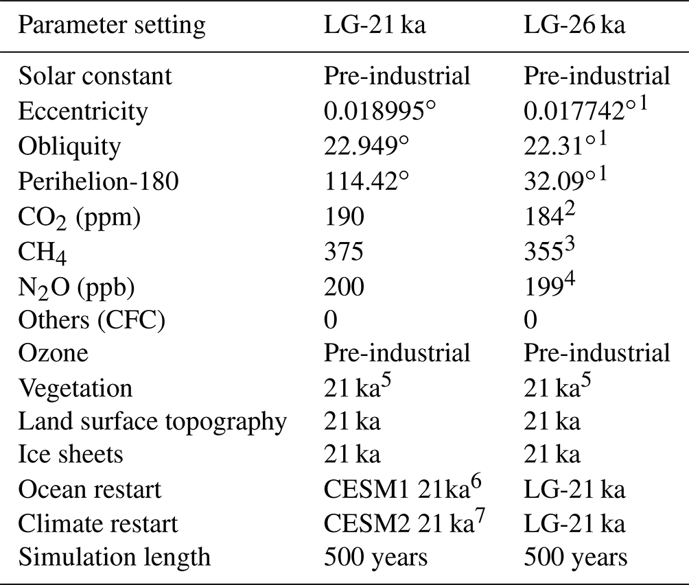
¹ Berger (1978). ² Bereiter et al. (2015). ³ Loulergue et al. (2008). ⁴ Schilt et al. (2010). ⁵ Offline BIOME4 simulation (Kaplan et al., 2003). ⁶ DiNezio et al. (2018). ⁷ Zhu et al. (2021).

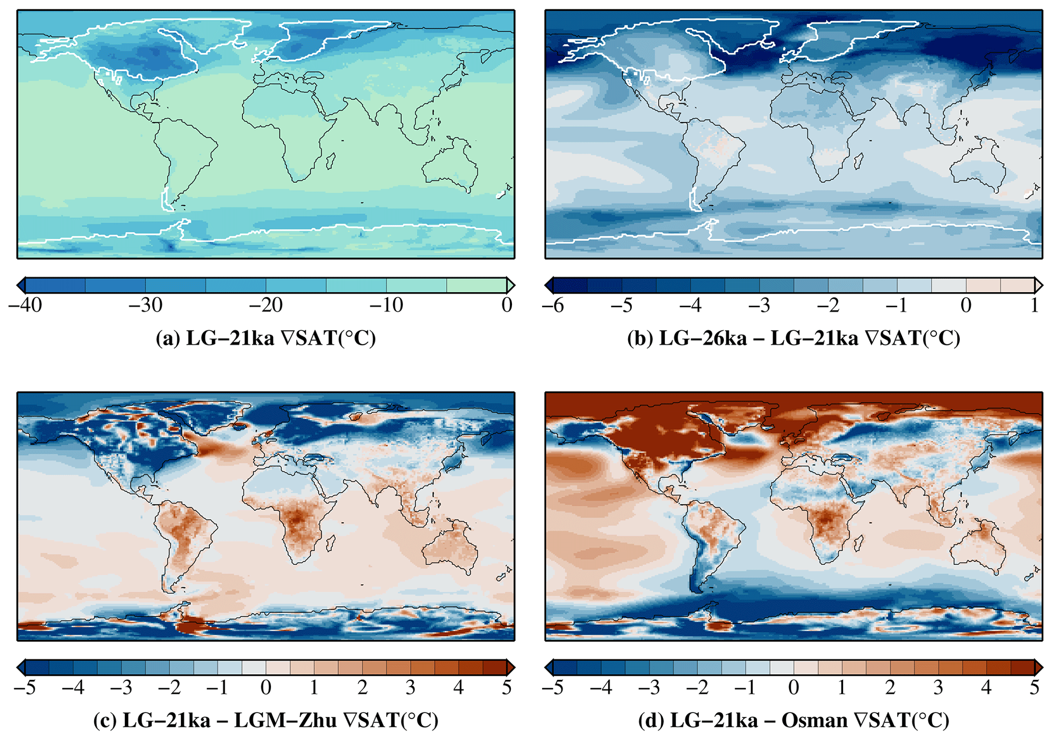
Figure 1 Annual–mean (20 years) near-surface air temperature (SAT in ^∘C) anomalies with respect to pre-industrial levels. Panel (a) shows the LG-21 ka simulation. The black contour is the paleo-coastline and the white contour encloses the glaciated regions. Panel (b) shows differences between LG-26 ka and LG-21 ka. Panel (c) shows differences between LG-21 ka and Zhu et al. (2021) henceforth referred to as “LGM-Zhu”. Panel (d) shows differences between LG-21 ka and SAT taken from Osman et al. (2021) (regridded to the CESM grid).

Table 2 Annual means (20 years) of various quantities from LG-26 ka and LG-21 ka, CCSM4 (Brady et al., 2013), PMIP4 (Kageyama et al., 2021), and different proxy data. Standard deviations are given in curly brackets and differences to their respective pre-industrial (PI) simulations in round brackets. Note that a latitudinal range of 30^∘ S to 30^∘ N was used for the tropical calculations.

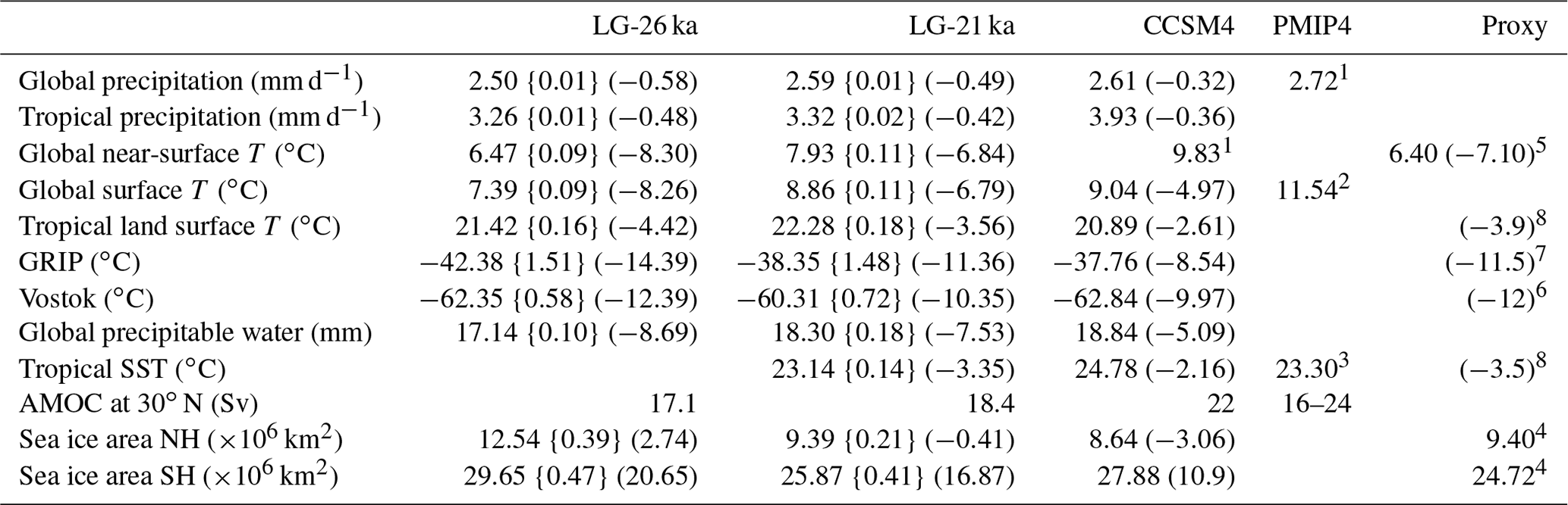
¹ AWI-ESM-1-1-LR, INM-CM4-8, MIROC-ES2L, MPI-ESM1-2-LR. ² MIROC-ES2L. ³ MIROC-ES2L, MPI-ESM1-2-LR. ⁴ Paul et al. (2021). ⁵ Osman et al. (2021). ⁶ Petit et al. (1999). ⁷ Lecavalier et al. (2014). ⁸ Tierney et al. (2020).

3 Climate simulation

To evaluate the climate state from our two simulations, we compare the global average of a range of climate outputs from LG-21 ka and LG-26 ka to published proxy and model results (Table 2). Additionally, we evaluate the spatial pattern of the global near-surface temperature (SAT) (Fig. 1), sea surface temperature (SST) and sea ice extent (Fig. 2) from LG-21 ka to a range of published datasets. For the SST and sea ice we have regridded the GLOMAP dataset (Paul et al., 2021) onto our CESM grid. However, we note that there is uncertainty in the GLOMAP sea ice data that has not been fully quantified and we are using it only as a guide to assess our simulations. For SAT we use two datasets: (i) an alternative 21 ka CESMv2.1 simulation (Zhu et al., 2021, refer to as LGM-Zhu) and (ii) proxy-constrained, full-field reanalysis from Osman et al. (2021) (referred to henceforth as “Osman”) (Fig. 1c and d). There are two differences in the model setup between the two CESMv2.1 21 ka simulations (LG-21 ka and LGM-Zhu): (i) the input vegetation dataset, with LGM-Zhu adopting a PI datasets all over the globe; and (ii) the ice sheet reconstruction, with LGM-Zhu using the ICE6G as defined within the PMIP4 protocols. In the ICE6G reconstruction, the GrIS is smaller and does not extend beyond the present day coastline and, as such, the adjustments made within POP in our model setup (see Sect. 2.1) are not required.

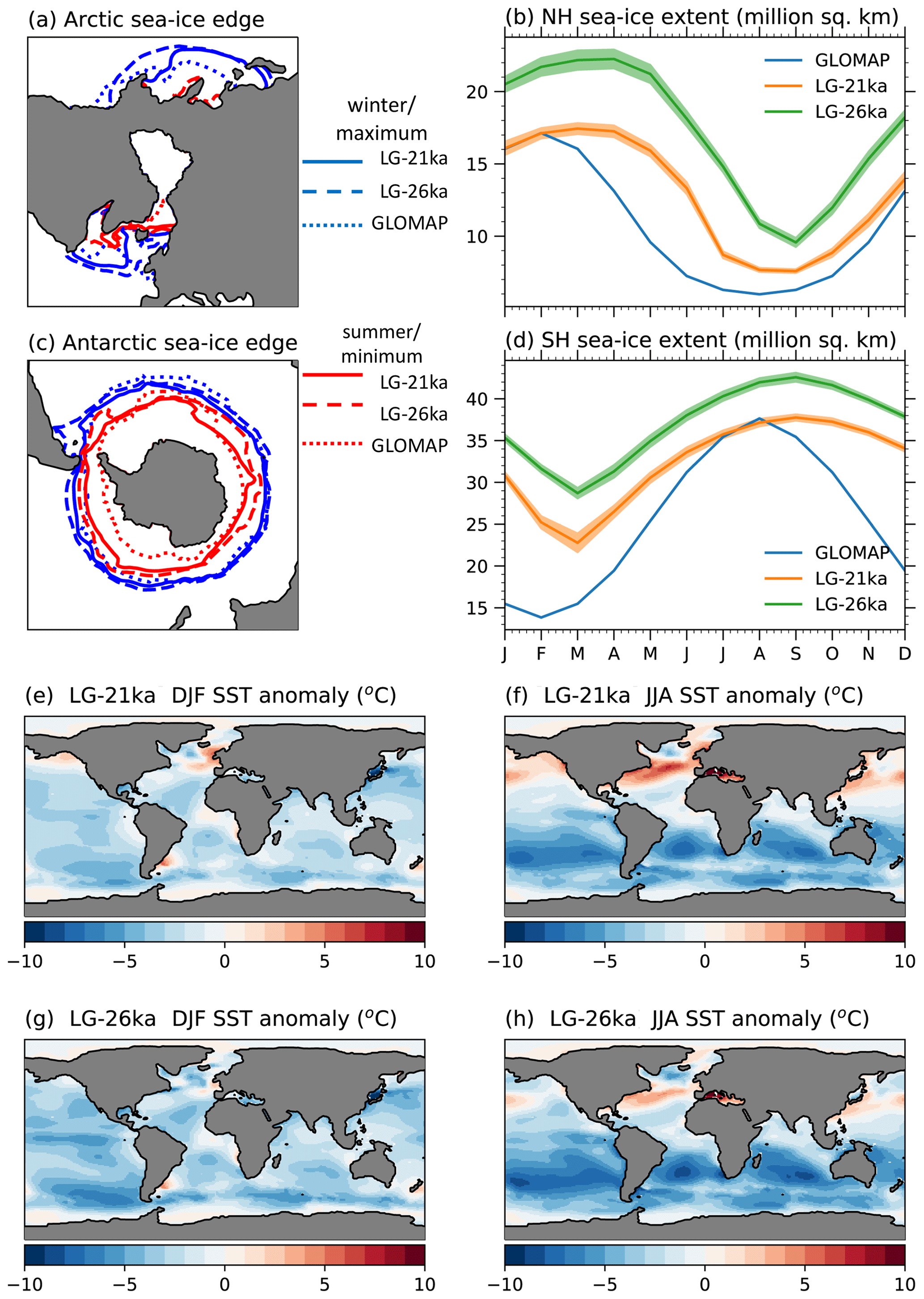
Figure 2 Comparison of sea ice and SSTs between LG-21 ka and LG-26 ka and GLOMAP (Paul et al., 2021). Panels (a, c) show sea ice edge (>15 % sea ice concentration) for the maximum/winter extent (blue) and minimum/summer extent (red), with LG-21 ka in solid lines, LG-26 ka dashed line, and GLOMAP dotted lines. Panels (b, d) show the mean (20 years) sea ice extent for the Northern and Southern hemispheres per month of the year. Panels (e)–(h) show the December–January–February (DJF) and June–July–August (JJA) SST anomalies (in ^∘C), where the anomalies are the difference between LG-21 ka and LG-26 ka and GLOMAP, and their respective pre-industrial values.

An average global near-surface cooling of 6.8 ^∘C is simulated by the LG-21 ka simulation (Fig. C1; Table 2), which agrees well with the results from the two comparison datasets: Osman 7.1±1 and 6.5 ^∘C LGM-Zhu and the recent study by Liu et al. (2023). This simulation is significantly colder (lower temperature) everywhere than the PI (Fig. 1), with the cooling amplified across the polar regions in both seasons (Fig. C2). The largest reduction in temperature (cooling) is across the glaciated regions (North America, Eurasia, and Antarctica) due to the higher elevations and the change from vegetated surfaces to ice surfaces (relative to the PI). This is in contrast to contemporary polar amplification, where the highest increases in winter near-surface temperatures take place over the Arctic Ocean.

When comparing the LG-21 ka results to LGM-Zhu and Osman, we find some notable spatial differences (Fig. 1c and d) in the SAT which approximately corresponds to the differences in elevation between the two simulations (Fig. C3). The lower (colder) temperatures around the margin of the ice sheet are associated with higher elevations (and vice versa). However, we note that it is not an exact 1-to-1 relationship. The differences across the surface of the large ocean basins are small, less than ±0.5 ^∘C, but as Sect. 3.2 describes, there are differences in the deep ocean circulation. Relative to the Osman study, LG-21 ka is colder across AIS and the southern ocean (up to 7 ^∘C) but is warmer across the central Pacific (up to 3.5 ^∘C), North Atlantic (up 11 ^∘C), and Arctic oceans (8 ^∘C). The largest warm anomalies are across the Northern Hemisphere ice sheet region: up to 20 ^∘C across the centre of the Cordilleran ice sheet (CIS) and 12 ^∘C across the Laurentide ice sheet (LIS). Note that these regions coincide with the highest standard deviations (up to 9 ^∘C) in the SAT from the ensemble of models performed by Osman et al., 2021). There is an anomalous cold zone extending from the southern coast of Greenland relative to both comparison datasets, the extent of which coincides with relatively large summer Arctic sea ice extent (Sect. 3.1).

The LG-26 ka simulation is 1.5 ^∘C colder than LG-21 ka (global average), enhanced at higher latitudes, with a 4 and 2 ^∘C cooling at the location of the GRIP and VOSTOK ice core sites. The largest anomalies are concentrated across the North Atlantic (decrease of 6 ^∘C) along the eastern margin of the GrIS and Siberia (decrease of up to 8 ^∘C) (Fig. 1b). In terms of the ice sheets, there is a cooling along the southern margin of the NAISC of 1 ^∘C, compared with 3 ^∘C across the BIIS, EuIS, and BKIS, which, as we evaluate in Sect. 4.1, has important implications for the simulated SMB.

3.1 Sea surface conditions

Both our simulations overestimate the mean monthly sea ice extent relative to GLOMAP (Fig. 2b and d; Table 2), with the area increasing in the colder temperatures of LG-26 ka and during the summer season. The timings of the Northern (Fig. 2b) and Southern Hemisphere (Fig. 2d) maximum and minimum sea ice extent are the same as for the present day but are delayed by 1 month relative to GLOMAP. Spatially, the differences are more complicated. During the summer in both the Northern and Southern hemispheres, LG-21 ka overestimates the spatial extent of the sea ice (Fig. 2a and c). For example, there are large areas of sea ice across the Norwegian and Greenland seas, which are ice free in GLOMAP. In the winter months, the simulation underestimates the sea ice in these regions, but it overestimates across the Bering Sea, Baffin Bay, and into the Labrador Sea.

Generally, LG-21 ka simulates colder ocean temperatures than GLOMAP (Fig. 2e and f) across large areas of the ocean, with the global mean SST −2.2 and −2.4 ^∘C colder in winter and summer, respectively. This colder ocean may be one cause for the consistent overestimation in the sea ice extent. There are warm anomalies (reaching up to 8 ^∘C), which are predominately concentrated in the Northern Hemisphere, extending from the NAISC across the North Atlantic Ocean to the BIIS and extending from the North Pacific Ocean (the Gulf of Alaska and Bering Strait) across to the Sea of Japan.

3.2 Atlantic meridional overturning circulation

The Atlantic meridional overturning circulation (AMOC) strength (defined as the maximum AMOC transport at 30^∘ N) is weaker, and the extent of the overturning cell is shallower in all three LGM simulations relative to the PI (Fig. 3b). The maximum strengths are 18.4, 17.1, and 16.6 Sv for LG-21 ka, LG-26 ka, and LGM-Zhu, respectively (Fig. 3b). As stated earlier, the LG-21 ka and LGM-Zhu simulations adopted different ice sheet reconstructions with the former including a revised overflow parameterization around Baffin Bay and Denmark Strait. A recent publication (Kapsch et al., 2022) found that the ICE6G reconstruction (similar to LGM-Zhu) resulted in a stronger AMOC relative to GLAC1D (similar to LG-21 ka) due partly to higher elevation across the NAISC complex. This is the opposite of the results from this comparison, which highlights the complex non-linear interplay between the change in elevation across glaciated regions and the resultant impact on sea ice extent and AMOC strength (Sherriff-Tadano et al., 2018; Sherriff-Tadano and Abe-Ouchi, 2020; Zhu et al., 2014). Two recent transient simulations for the LGM period found either no change in the AMOC between 26 and 21 ka BP (Kapsch et al., 2022) or a minor weakening (Quiquet et al., 2021), which is similar to our findings.

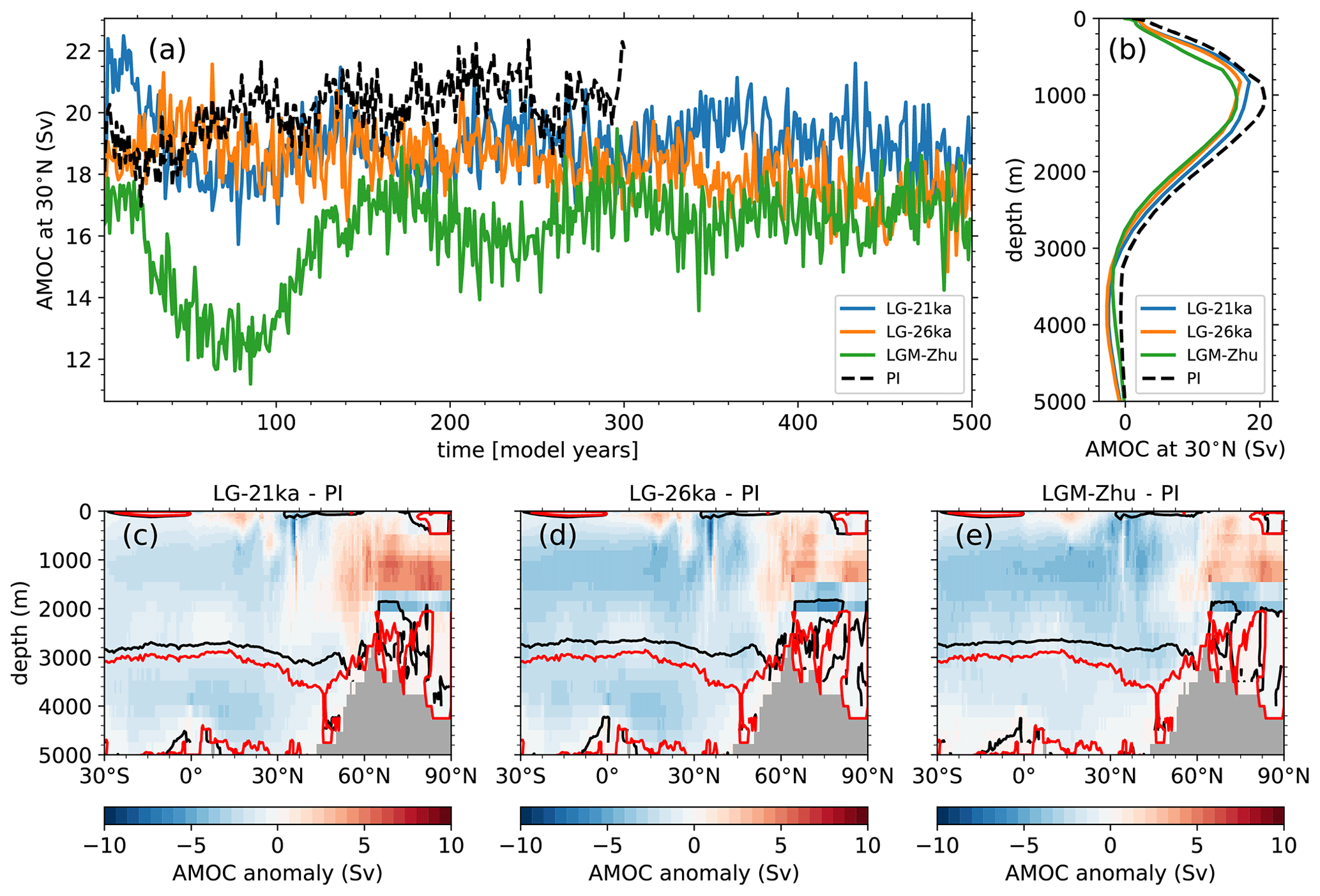
Figure 3 AMOC strength (defined as the maximum AMOC transport at 30^∘ N) as a function of (a) time and (b) depth for LG-21 ka (blue line), LG-26 ka (orange line), LGM-Zhu (green line), and PI (black line). Panels (c–e) show the AMOC anomaly as a function of latitude and depth (in Sv; 0 Sv contour line in black for LG-21 ka and red for PI) for (c) LG-21 ka, (d) LG-26 ka, and (e) LGM-Zhu with respect to the PI simulation. Values in (b)–(e) are averaged over the past 20 years of each simulation.

The maximum extent of the overturning cell, defined as the depth for which the AMOC strength (at ∼30^∘ N) is positive, shoals by ∼240 m for LG-21 ka and LG-26 ka and by 480 m in LGM-Zhu (Fig. 3b). The shoaling of the simulated glacial AMOC compared with the PI simulation is in agreement with most of the earlier LGM studies (e.g. Muglia and Schmittner, 2021; Gu et al., 2020).

Evaluating the AMOC strength from a depth–latitude viewpoint (Fig. 3c, d, and e), south of ∼50^∘ N the AMOC is weaker and shallower in all three LGM simulations (LG-21 ka, LG-26 ka, and LGM-Zhu), while north of ∼60^∘ N its signal is stronger and of similar vertical extent. Therefore, some of the differences between various studies may result from not adopting the same definition for the AMOC. Previous studies have suggested that the process of deep convection in the Labrador Sea is affected by the advancing of the sea ice in the lower temperatures of the glacial climate which, in turn, impacts the AMOC strength and geometry (Klockmann et al., 2018). As stated above, this is a region where LG-21 ka overpredicts the extent of the sea ice (Fig. 2a). Indeed, the winter mixed layer depth averaged over the subpolar North Atlantic is shallower by ∼400 m in the glacial simulations compared with the PI (Fig. C5a, b, and c). Therefore, our weaker AMOC may result from the overestimation of sea ice which limits the deep water formation producing a weaker overturning cell compared with the PI. In the Nordic seas, north of ∼60^∘ N, the winter mixed layer depth is deeper in the glacial simulations compared with the PI (Fig. C5a, b, and c) which corresponds to the region of stronger AMOC ∼60^∘ N (Fig. 3c, d, and e).

3.3 Atmospheric simulation: radiation, clouds, and circulation

The LG-21 ka simulation top of the atmosphere (TOA) SW_in is reduced (less insolation) with respect to the PI at northern and southern high latitudes during May–October and October–March, respectively (Fig. 4a). Tropical and subtropical regions experience a small positive change in insolation for most months, except between August and October where they have a small negative change in insolation. During these periods of reduced TOA SW_in (−10 W m²), there is a much larger increase in the surface SW_in (Fig. 4b), up to 100 m², which can be linked primarily to changes in the cloud cover (Fig. 4c). Additionally, the presence of the extensive LGM ice sheets (Fig. A1) combined with the increase in the spatial extent of sea ice into the mid latitudes (see Sect. 3.1) increases the surface albedo (see Fig. 8f) which allows more multiple scattering and therefore also contributes to the increase in the surface SW_in. In all high latitude regions showing enhanced surface SW_in, SW_net (Fig. 4d) is reduced due to overcompensation from higher surface albedo (Fig. 8f).

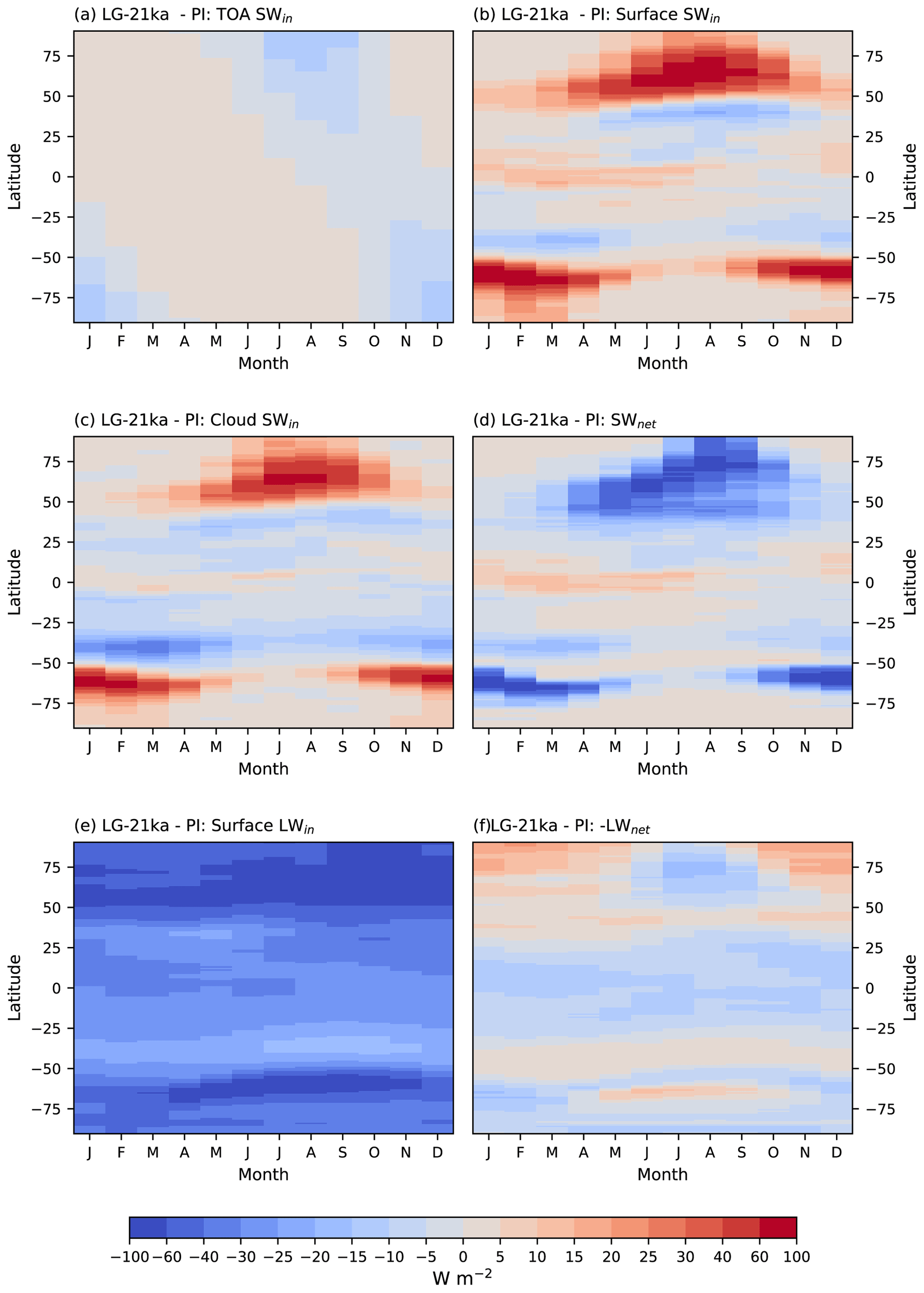
Figure 4 Monthly zonal means (20 years) of (a) top of the atmosphere (TOA) incoming solar radiation (SW_in), (b) incoming solar radiation at the surface (SW_in), (c) cloud contribution to incoming solar radiation at the surface (SW_in), (d) net shortwave radiation at the surface (SW_net), (e) incoming longwave radiation at the surface (LW_in), and (f) net longwave radiation at the surface (LW_net). For all panels, positive values (red) indicate energy gain by the surface. Total radiation change at the surface results from the addition of (c) and (e).

The surface incoming longwave radiation (LW_in; Fig. 4e) is reduced at all latitudes and times of the year with respect to the PI with the largest anomalies corresponding to the areas of largest cooling over the ice sheets (Fig. 1a)and expanded sea ice cover. The temporal and latitudinal pattern of surface net longwave radiation (LW_net; Fig. 4f) shows both positive and negative anomalies (positive corresponds to net radiation gain by the surface), with net radiation loss over the Northern Hemisphere ice sheets during the summer and, in the tropics, all year long. The magnitude of this summer reduction in LW_net over the ice sheets is smaller than for SW_net.

We continue our analysis of atmospheric change by examining changes in the atmospheric circulation (asymmetrical component of the geopotential height) and their connections with cloud change (Fig. 5). Around the NAISC, two circulation anomalies appear (Fig. 5a and b). On the western coast of North America across the CIS, the PI winter ridge is intensified and extends further towards Asia. The winds associated with this ridge transport warm and moist air from the Pacific to Alaska. Across the east coast of North America and the LIS, a negative response occurs, due to the strengthening and southward elongation of the Greenland climatological low, extending the persistent inflow of Arctic air towards the North Atlantic margin. This response strengthens the geopotential gradient between the Atlantic and LIS, suggesting higher wind speeds of the polar jet.

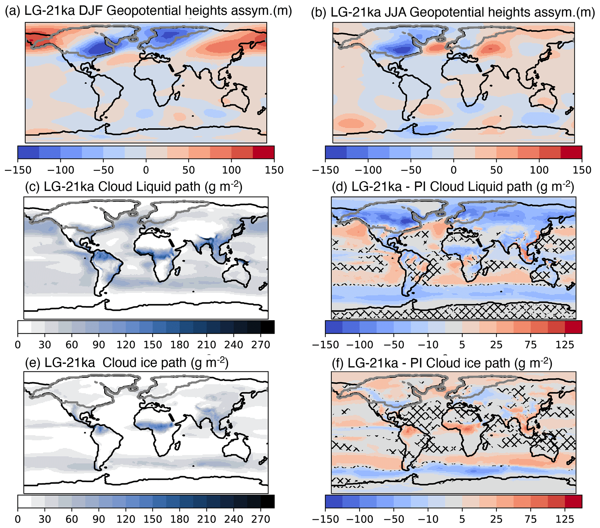
Figure 5 Geopotential height anomalies (relative to the PI; in metres) after subtracting the zonal means (20 years) for (a) DJF and (b) JJA. Note that we analyse the geopotential height at an atmospheric pressure of 200 hPa. Panels (c)–(f) are relative to the Summer mean clouds. Panels (c) and (d) show cloud liquid path, while (e) and (f) show cloud ice path, all in g m⁻². The left column shows values from the LG-21 ka simulation, while the right column shows the differences between LG-21 ka and the PI simulations. The grey contour encloses glaciated areas (>50 % ice cover). Patched areas show where differences are non-significant at the 99 % level according to a Student's t test relative to the month variations.

The winter climatological ridge (Fig. 5a) which brings warmer and moister air from the North Atlantic towards Europe is weakened along its northern flank, which results in drier and colder Arctic air over northern Europe. On the Asian side, the Aleutian low is weakened. The summer circulation responses (Fig. 5b) are weaker than in winter. There is a negative response over the LIS, which represents a narrowing of the Rocky Mountain ridge and a strengthening and enlarged Greenland low. This change in summer circulation results in a reduction in temperature across the LIS during the LGM (Fig. 1a). There is a positive response in the North Atlantic which extends across the BIIS. As both these responses strengthen the PI climatological features, they sharpen the geopotential gradients and give rise to higher wind speeds, which is indicative of increased synoptic eddy activity. The circulation anomalies in LG-26 ka are very similar which suggests they are not strongly influenced by the changes in orbital forcing.

To investigate further the influence of clouds on the radiation fluxes, we examined the change in cloud liquid and ice content (Fig. 5d and e). Clouds with a higher liquid content will block incoming solar radiation, whereas ice is nearly transparent to incoming solar radiation. During the summer, there is very little cloud liquid water across the ice sheets (Fig. 5c), a significant reduction compared with the PI (Fig. 5d). This is caused by the increase in elevation, a relatively high cloud liquid water in the PI, as well as the negative circulation anomalies (Fig. 5b) making these areas receive more dry and cold Arctic air. Therefore, the positive anomalies in the SW_in (Fig. 4a) are in part due to a reduction in cloud liquid. Conversely, there is a small increase in cloud ice water (Fig. 5e and f), a feature that is common over current ice sheets, due to the colder temperatures and higher elevation (Ettema et al., 2010; Lenaerts et al., 2019).

In summary, we see large differences in circulation, clouds, temperature, and precipitation between the LG-21 ka and PI climates, some of them largely connected with the presence of large ice sheets in the Northern Hemisphere. The circulation in LG-21 ka suggests more advection of Pacific air towards Alaska, bringing more moisture which increases precipitation and thickens clouds. In the interior of the NAISC (across the Laurentide ice sheet) there is an anomalous trough, which likely brings in drier Arctic air, leading to thinning of clouds, less precipitation, and much lower air temperatures than in the PI. In LG-21 ka the temperatures are lower around Greenland, particularly in the west where the PI low gets strengthened. The Eurasian ice sheets experience similar responses to those of the Laurentide: wetter in the south and drier in the interior and north.

4 Northern Hemisphere ice sheet surface mass and energy balance

In the following, we will compare the SMB and summer surface energy balance and their components across the main continental scale Northern Hemisphere ice sheets. We distinguish between six ice sheets: NAISC, GrIS, BKIS, SIS, BIIS, and Icelandic (IcIS). The summer energy balance is analysed to identify the different contributions from incoming solar and longwave radiation, albedo, and turbulent heat fluxes to melt energy. In the last subsection, we compare the results of LG-26 ka and LG-21 ka.

4.1 Surface mass balance and components per ice sheet

Figure 6 shows a comparison of the spatially averaged SMB and its components across the six major Northern Hemisphere ice sheets with the corresponding values for the present-day ice sheets of Greenland (Noël et al., 2020) and Antarctica (Mottram et al., 2021). Average values have been chosen to compare different ice sheets regardless of their different areas.

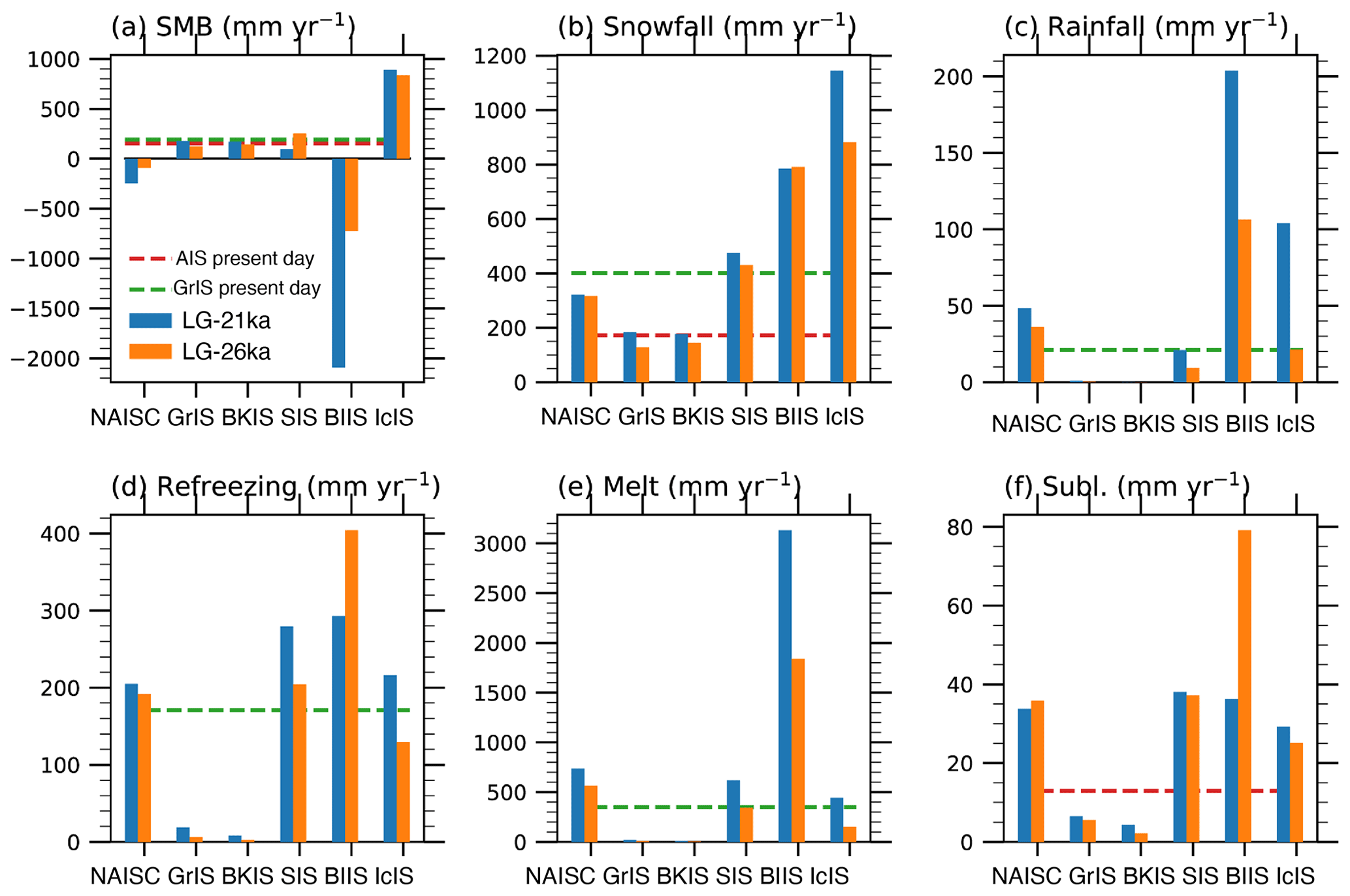
Figure 6 Annual means from the past 20 years of simulation of (a) surface mass balance, (b) snowfall, (c) rainfall, (d) refreezing, (e) melt, and (f) sublimation, all in mm yr⁻¹. Blue bars represent LG-21 ka averages and orange bars represent LG-26 ka averages, over the individual ice sheets. North American ice sheet complex (Laurentide, Cordilleran, and Innuitian; NAISC), Greenland ice sheet (GrIS), Barents–Kara Sea ice sheet (BKIS), Scandinavian ice sheet (SIS), British–Irish and North Sea ice sheet (BIIS), and Icelandic ice sheet (IcIS). The dashed green and red lines correspond to present-day GrIS and AIS averages (Mottram et al., 2021; Noël et al., 2020). Note that the annual means are scaled by ice sheet area (in units of mm yr⁻¹).

The averaged SMB of the IcIS, SIS, GrIS, and BKIS is positive, with the latter two results of similar value to present-day Greenland and Antarctica (around 200 mm yr⁻¹). The similarity in the simulated mean GrIS SMB is the result of the almost zero melt rate (Fig. 6e) at the LGM combined with the ∼50 % reduction in the snowfall rate (200 mm yr⁻¹ at the LGM versus 400 mm yr⁻¹ for present day; Fig. 6b). These differences in the SMB components are associated with the lower temperature and drier LGM climate (Fig. 1).

The LG-21 ka GrIS excluding the wetter southeast margin (Fig. 7b) and BKIS have similar mean SMB and components: low snowfall rates, zero rainfall and melt (except for a narrow band in southwest Greenland), and interiors with low net snow deposition (Fig. 7b) contrasting with low sublimation-dominated margins (Fig. 7f). All other ice sheets have large areas of melt which largely correspond with the relatively wide ablation areas (Fig. 7a and e). The SIS has a mean SMB that is half of the BKIS, regardless of more than double the snowfall rates (Fig. 6b), with a value very similar to that of present-day Greenland. This is due to relatively large melt rates (almost double than for present-day Greenland). The SMB of the IcIS is the largest of all the six ice sheets, due to a very high snowfall rate (Fig. 6b) that is only partially compensated by melt rates of a similar magnitude to those of present-day Greenland.

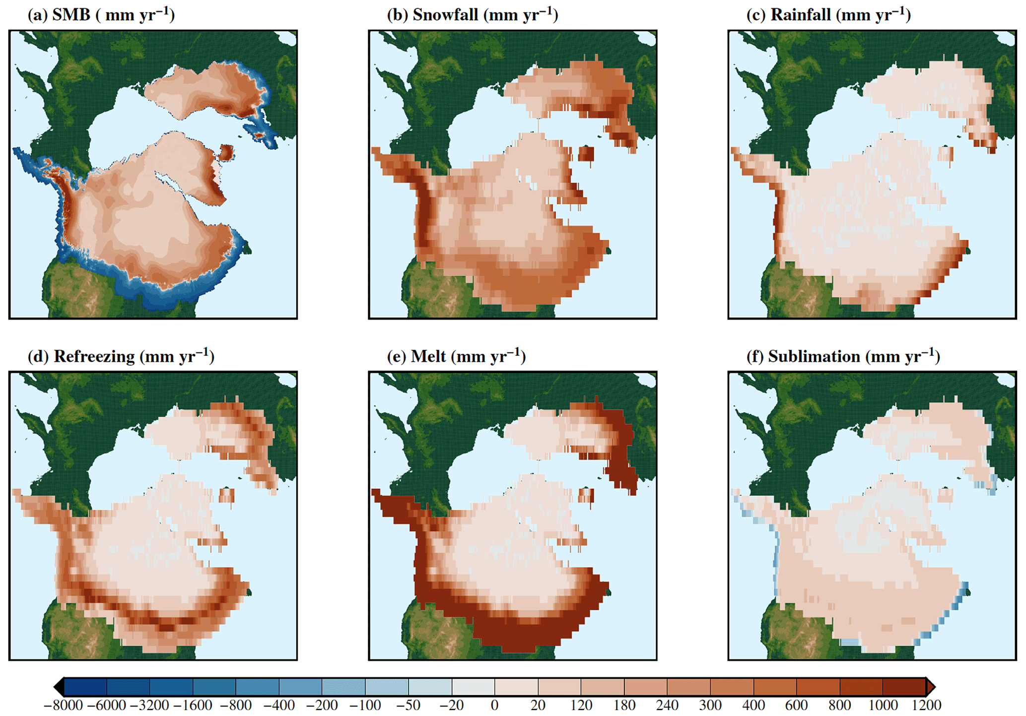
Figure 7 Maps of LG-21 ka annual means from the past 20 years of simulation of (a) surface mass balance (downscaled onto the higher resolution CISM2.1 4 km grid; Fig. A1), (b) snowfall, (c) rainfall, (d) refreezing, (e) melt, and (f) sublimation, all in mm yr⁻¹.

Two ice sheets have an extremely negative SMB across the ablation area: NAISC and BIIS. The CIS, which is part of the NAISC, has a wide ablation area along the southern and western (Pacific) margins, with the latter corresponding to the high snow accumulation rates over the high elevation of the Sierra Nevada mountain range (Fig. 7b). For the LIS, the high ablation and melt area extends along the entire southern margin, even over the relative high elevation of the southern (Atlantic) margin, due to the relatively high summer temperatures (Fig. C2). High refreezing rates are simulated along the equilibrium line altitude, at the transition between the accumulation and ablation zone along the southern margin (Fig. 7d). Both these ice sheets (CIS and LIS) have high rainfall rates and inverse sublimation (or snow deposition) along the marine terminating margins not bordered by sea ice (see Fig. 2a), with mean values more than double present-day Greenland and Antarctica, respectively (Fig. 6c and f). The BIIS has the lowest mean SMB of the six ice sheets, despite having the second largest snow accumulation. The simulated ablation areas cover most of the ice sheet except for a minimal accumulation area in the interior, across the higher elevation of Scotland (Fig. 7a). The entire ice sheet surface melts seasonally (Fig. 7e), with average melting rates almost an order of magnitude larger than for present-day Greenland.

If the simulated SMB, including the very wide and negative ablation area of the NAISC and BIIS, was applied to a dynamic ice sheet model (for example, CISM2.1; Lipscomb et al., 2019), it would be highly unlikely/challenging that the spatial extent of the southern margin in either ice sheet would be maintained; rapid retreat would likely occur. However, as outlined in Sect. 1, the timing of the LGM for both these ice sheets was earlier than the historical 21 ka BP definition (25 ka BP for NAISC and 23 ka BP for BIIS). Therefore, an earlier time step in this 6 ka period may be more appropriate to simulate the glacial maximum for these ice sheets. For this reason, in Sect. 4.3, we compare the LG-21 ka simulation with LG-26 ka.

4.2 Melt sources: the surface energy budget

Here we will examine the components for the summer (JJA) energy budget over all Northern Hemisphere ice sheets (Fig. 8). Melt is simulated across all margins of the major six continental ice sheets (Fig. 8a) apart from those bordered by sea ice (Fig. 2), for example, the BKIS, the eastern margins of GrIS, and the arctic sea margin of the LIS.

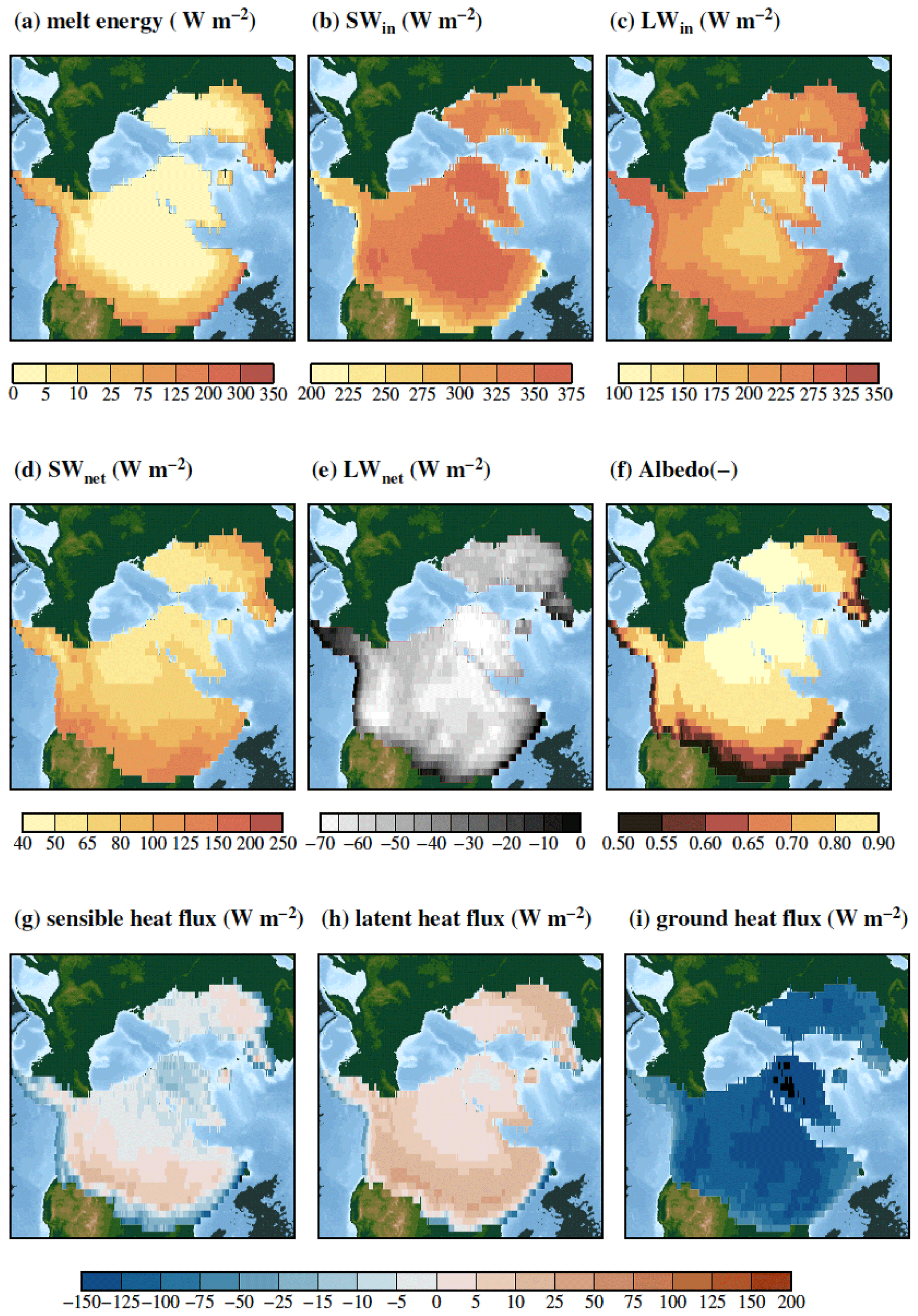
Figure 8 Maps of LG-21 ka summer (JJA) means from the past 20 years of simulation of (a) melt energy, (b) SW_in, (c) LW_in, (d) SW_net, (e) LW_net, (f) albedo, (g) sensible heat flux, (h) latent heat flux, and (i) ground heat flux.

Incoming solar radiation is high in the interior of the NAISC, GrIS, and SIS with much lower rates at the margins (Fig. 8b). Minimum incoming solar radiation is simulated over the southern and Atlantic margins of the NAISC and over the BIIS, due to higher amounts of cloud water over those ablation areas. An increase in shortwave radiation towards the higher elevation in the interior of ice sheets is also a feature of the present-day GrIS (van den Broeke et al., 2008) and is simulated by regional (Ettema et al., 2010) and global climate models (van Kampenhout et al., 2020; Vizcaíno et al., 2013; Dunmire et al., 2022). Conversely, maximum incoming longwave radiation is simulated over the margins which have higher temperatures, except for northern North America, GrIS, and BKIS (Fig. 8c). Compared with the PI simulation, across the ice sheets there is an increase in cloud fraction (i.e. gets cloudier), but the clouds are thinner. These two specific changes in the nature of the clouds can be related to the earlier responses in the radiation fluxes (see Sect. 3.3). Thinner clouds act to increase the incoming solar radiation at the surface (Fig. C4a). Conversely, in cloudier areas, the clouds increase the incoming longwave radiation, although the clouds are thinner (Fig. C4g and h).

Summer surface albedo (Fig. 8f) is minimum (between 0.5 and 0.55) over the ablation areas corresponding to bare ice exposure. The highest albedo values (>0.80) correspond to dry snow areas extending from northern Canada, where the LIS and Innuitian ice sheet (IIS) coalesce, into central and southeastern Greenland, the interior of IcIS, and most of the BKIS. The combination of this spatial albedo pattern and the reduction in incoming solar radiation over the ablation areas (Fig. 8b) results in maximum net solar radiation over the southern regions of the NAISC and SIS ice sheet margins (Fig. 8d). The sensible heat flux (SHF) provides energy for the surface over most of the ablation areas and all over Greenland. The largest flux towards the atmosphere is simulated at intermediate elevations, just above the equilibrium line altitude of the southern half of the NAISC. The latent heat flux (LHF) is positive (directed towards the surface) over a somewhat narrower band than the sensible heat flux along the lowest part of the ablation areas and is negative over the rest of the ice sheets. The positive LHF anomaly along the southern margin of the ice sheets is due to prolonged bare-ice exposure, whereas when relatively warm and moist air is advected over this region condensation occurs (Sellevold and Vizcaíno, 2020). The ground heat flux (GHF) provides energy to the surface along the areas with maximum refreezing (cf. Figs. 7d and 8i), due to the heat released in the refreezing process.

4.3 LG-26 ka versus LG-21 ka surface mass balance

The LG-26 ka simulation results in an SMB increase with respect to LG-21 ka for the NAISC, BIIS, and SIS (Figs. 6 and 9a), with the largest absolute difference for the BIIS. However, for the NAISC and BIIS this does not reverse the SMB sign, which if applied to an offline ice sheet dynamical model would likely initiate retreat. This increase in the SMB is primarily caused by a reduction in the melt rates (Figs. 6e and 9e). Over the BIIS, a small increase in snowfall contributes secondarily to higher SMB and is related to a cooling-related reduced fraction of precipitation falling as rainfall (Figs. 6c and 9b). Gandy et al. (2018) concluded that a warming of the climate after 26 ka, and the resultant reduction in SMB, was in fact required to initiate the retreat of the BIIS at 21 ka. Therefore, the 1.5 ^∘C warming between LG-26 ka and LG-21 ka due to the change in orbital parameters may be one factor that led to the retreat of the BIIS, due to the increase in melt rate (Fig. 6e).

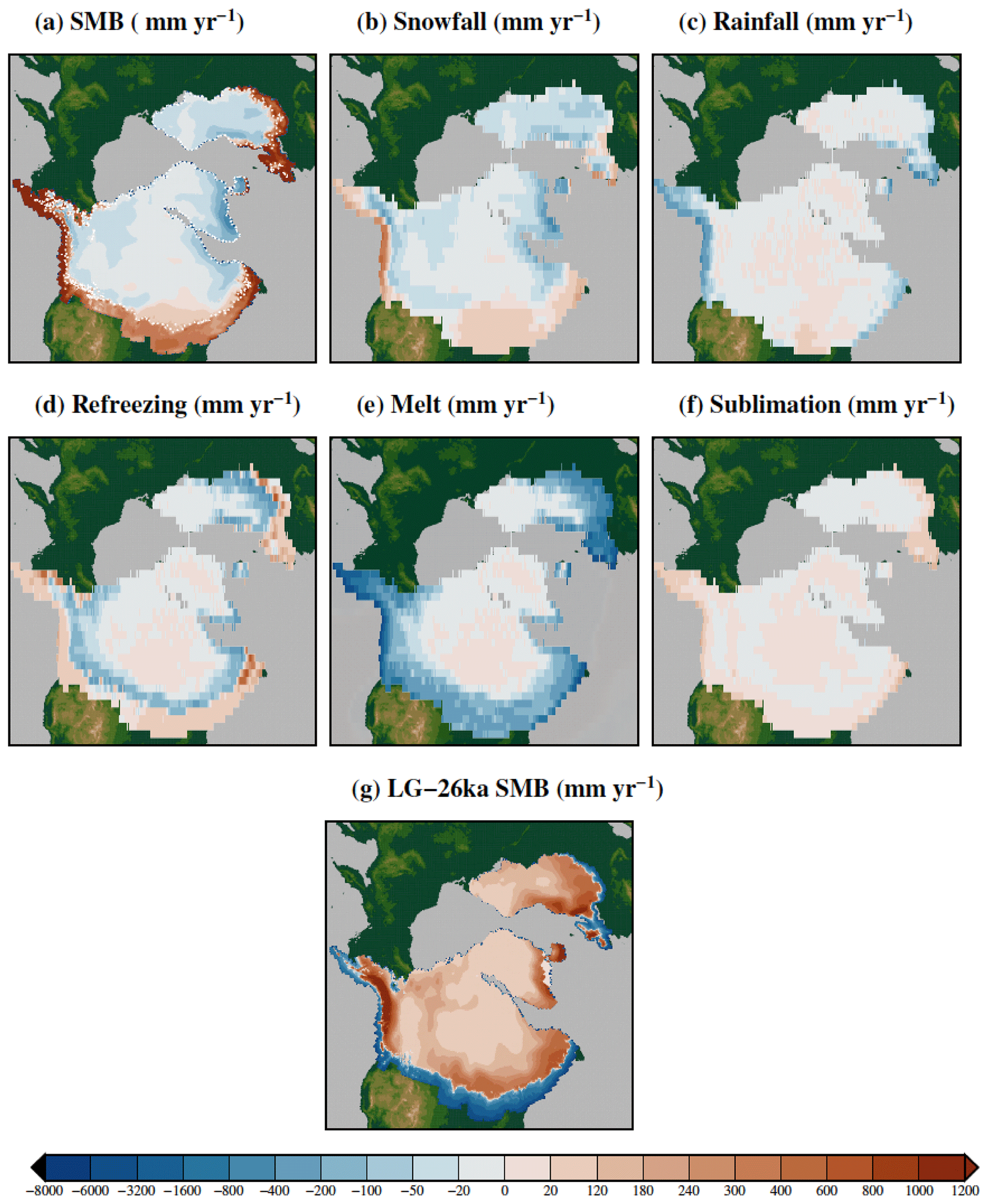
Figure 9 The difference between the results of the LG-26 ka and LG-21 ka (annual means from the past 20 years of each simulation). Panel (a) shows surface mass balance, (b) snowfall, (c) rainfall, (d) refreezing, (e) melt, and (f) sublimation, all in mm yr⁻¹. Panel (g) shows surface mass balance for LG-26 ka (downscaled onto the higher resolution CISM2.1 4 km grid (Fig. A1).

Over the other five ice sheets, snowfall rates are lower in the LG-26 ka simulation compared with LG-21 ka. Mean rainfall rates decrease over all ice sheets, apart from the two driest (GrIS and BKIS) where it remains almost zero. The largest reduction is over the ice sheets with a prominent North Atlantic climate (BIIS and cIS).

The SMB is lower in LG-26 ka with respect to LG-21 ka for the two ice sheets with almost zero melt (GrIS and BKIS) and the IcIS, which has relatively low average melt rates. This decrease is due to reduced snowfall (Fig. 6b). A fall in melt rates at LG-26 ka results in a refreezing reduction over all ice sheets except for the BIIS, where the combination of a large reduction in melt and rainfall and a minor increase in precipitation results in an increase in refreezing (Figs. 6d and 9d). Spatially (Fig. 9a), the SMB increases over the ablation areas and decreases in the accumulation areas, the latter being due to reductions in snowfall (Fig. 9b). Snowfall increases and rainfall decreases along the western margin of the NAISC in connection with colder temperatures (Fig. 1b). Refreezing increases over the ablation areas in connection with a cooling-induced increase in the refreezing capacity, and decreases over the percolation areas, as a result of the reduction in melt (Fig. 9d and e).

5 Discussion and conclusions

Here we present for the first time a detailed, explicit analysis of climate, SMB, and energy components over Northern Hemisphere ice sheets, with a similar approach to that adopted for modern ice sheets with regional climate models (Ettema et al., 2010, 2009; Noël et al., 2018, 2020) and projections with global climate models (Muntjewerf et al., 2020a). This detailed analysis of surface mass and energy components is meant to facilitate an advanced comparison of climate and ice sheet simulations between (multiple) past and future time periods. A direct evaluation of our simulated SMB and components is not straightforward as there are no direct proxies available for the LGM, except for snow accumulation rates over the GrIS. Therefore, here we will briefly compare our results with those of Kapsch et al. (2021), who presented results of the spatial distribution of the SMB of the Northern Hemisphere ice sheets during the last deglaciation. In their study, they downscale their results to two different ice sheet reconstructions: ICE6G (Peltier et al., 2015) and GLAC1D (Tarasov et al., 2012). Our simulated LG-21 ka SMB spatial distribution is largely similar to that of Kapsch et al. (2021) downscaled onto the GLAC1D topography (this topography is the same for the NAISC in both studies) (Fig. 7; Fig. 4 in Kapsch et al., 2021). The simulation over common accumulation areas is very similar, with precipitation maxima over the CIS and southwestern Laurentide and southern SIS, and minima over present-day Hudson Bay, the northern half of Greenland, and the BKIS. The width of our ablation areas is difficult to compare as we present results on the climate (land component) grid, whereas the results of Kapsch et al. (2021) are on a higher-resolution grid. However, in general, the distribution of ablation areas is very similar, with the major discrepancy being that we have a larger ablation area for the BIIS than in their case. This discrepancy is smaller if we compare with their SMB downscaled to the ICE6G reconstruction (their Fig. A2). For the SIS and BKIS, our ablation area simulation is closest to that of Kapsch et al. (2021) downscaled to the GLAC-1D topography.

Our simulated SMB for the NAISC and BIIS appears too negative to prevent large marginal retreat if used as forcing for an ice sheet dynamical model. The possible causes of this low SMB are: (a) biases in the climate and/or snow/firn simulation, (b) biases in the ice sheet reconstruction (as the SMB is largely dependent on surface topography), and/or (c) climate and SMB conditions largely out of equilibrium during the LGM. A recent study by Gandy et al. (2023) also investigated the LGM NAISC in a coupled climate ice sheet model “FAMOUS-ice”. That study found that when initiating their simulations from a large NAISC (as adopted in this study), a large ablation area formed across the southern margin of ice sheet, which led to rapid ice sheet retreat (see Fig. 3 in Gandy et al., 2023). This behaviour was attributed to the heavy tuning of their model to present-day Greenland. As the CESMv2.1 model has also been shown to have problems when applied to the LGM climate (Zhu et al., 2021) and required de-tuning to comply with LGM global mean surface temperature constraints. Future work investigating coupled ice sheet–climate simulation for the LGM with CESMv2.1 may also require de-tuning to correctly simulate the LGM Northern Hemisphere ice sheets.

Appendix A: Ice sheet reconstruction

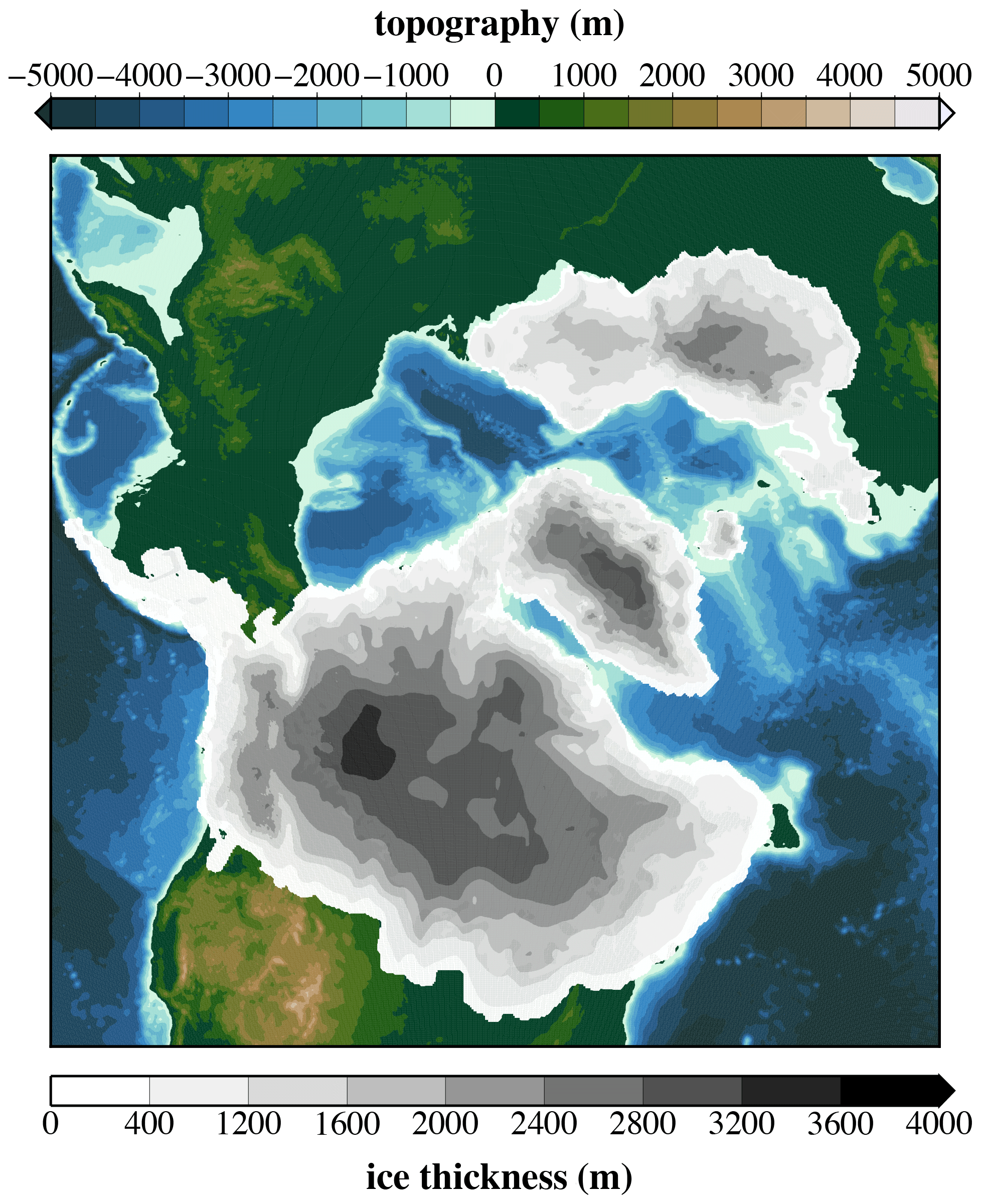
Figure A1 Ice sheet reconstructions used for simulations LG-21 ka and LG-26 ka at the finer CISM2.1 grid that is used for the elevation class calculations of the surface mass balance. The reconstruction combines the Antarctic and Patagonia ice sheets from ICE5G (Peltier, 2004), the North American ice sheet complex (Laurentide, Cordilleran, and Innuitian) (Tarasov et al., 2012), Greenland ice sheet (Lecavalier et al., 2014), and the Eurasian ice sheet complex (British and Irish, Scandinavian, and Barents–Kara Sea) from BRITICE-CHRONO (Clark et al., 2021).

Appendix B: Generation of input for the paleo-vegetation dataset

An offline vegetation model (BIOME4, https://github.com/jedokaplan/BIOME4; last access: October 2019); Kaplan et al., 2003) was run using climate forcing of LG-21 ka simulation to generate an LGM vegetation distribution. This simulated LGM vegetation distribution was combined with a present-day vegetation dataset as follows:

1. The CLM5 standard present-day vegetation dataset (Lawrence et al., 2019) is prescribed over the Southern Hemisphere and at low latitudes in the Northern Hemisphere. In these locations, the present-day vegetation is extrapolated over LGM emerged land using a nearest-neighbour mapping algorithm.

2. At higher latitudes in the Northern Hemisphere (north of 35^∘ N in Europe and Asia, North of 20^∘ N in North America) we prescribe an LGM vegetation based on the BIOME4 stand-alone simulation, which is run on a 0.5^∘ global grid and is forced with

   • monthly-averaged 2 m temperature, precipitation, and cloudiness for the past 20 years of a 90-year-long CESM2 LGM simulation using the standard present-day vegetation dataset;

   • LGM CO₂, and orbitals (as in the CESM2 LGM simulation 21 ka);

   • LGM soil properties dataset, provided as a personal communication by Jed O. Kaplan, October–November 2019.

The LGM BIOME4-simulated vegetation types are converted into CLM5 plant functional types (PFTs) following the conversion Table 2.1 in Oleson et al. (2013). Moreover, the following additional corrections are applied:

• Boreal broadleaf deciduous shrubs and boreal grass are prescribed over the Siberian continental shelf.

• Tropical broadleaf evergreen trees north of 20^∘ N have been converted to temperate broadleaf evergreen trees.

In Fig. B1, we show maps of the PFT percentage in the hybrid LGM/present-day vegetation dataset, and in Fig. B2 we show the output of the LGM BIOME4 simulation.

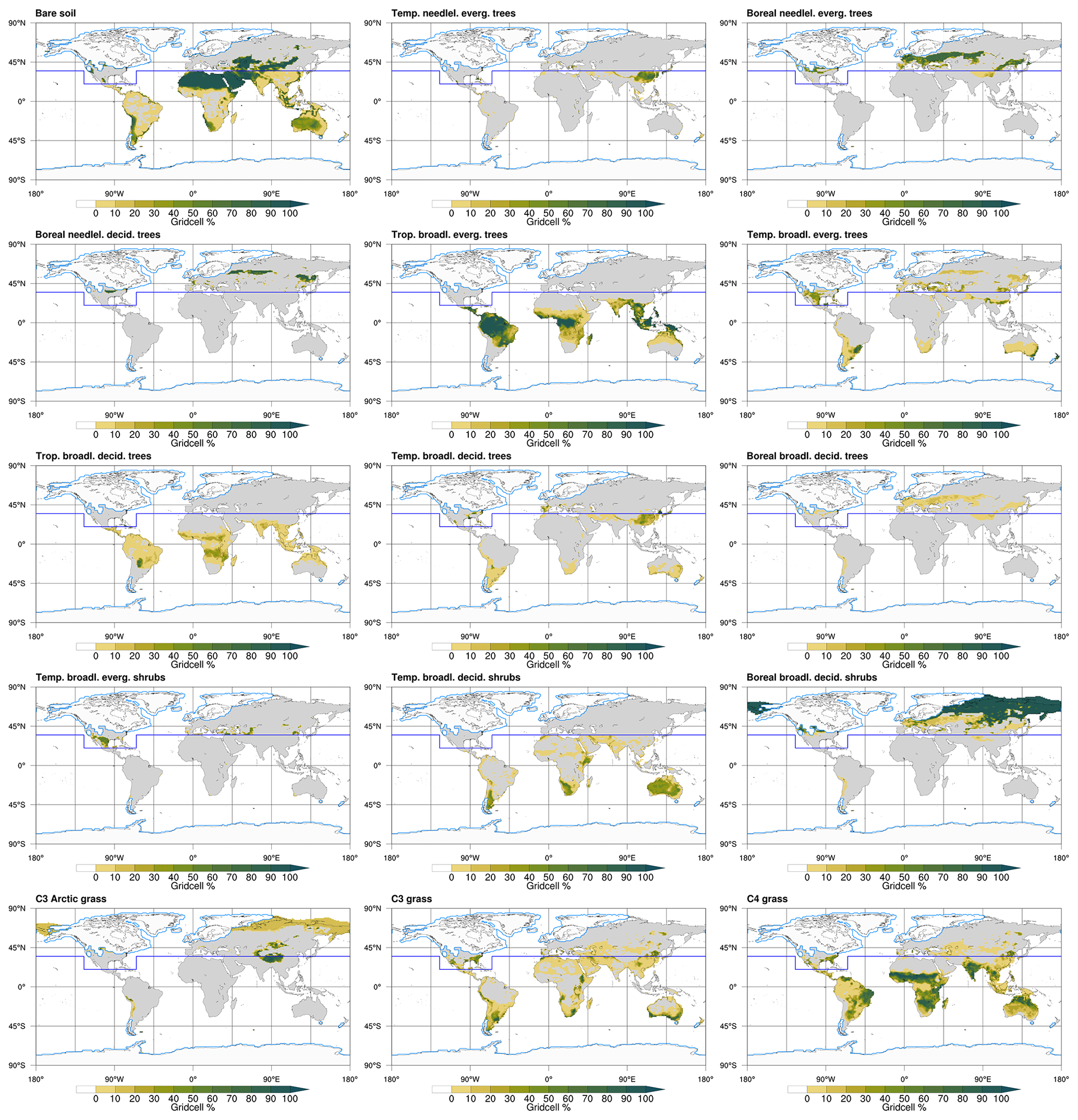
Figure B1 Global map of percentage of land cover, for each CLM5 plant functional type (PFT), in the hybrid LGM/present-day vegetation dataset. The dark blue line indicates the latitude limit above which the LGM BIOME4-based vegetation is used, instead of the standard CLM5 present-day vegetation dataset (which is prescribed below the latitude limit).

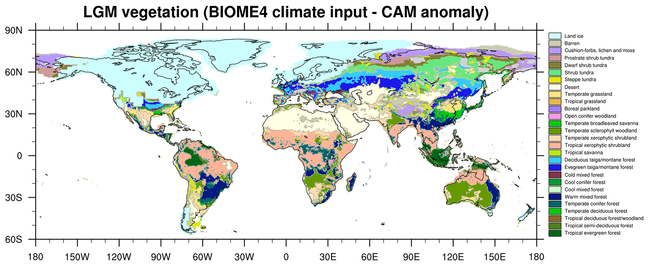
Figure B2 Simulated vegetation types in the BIOME4 stand-alone simulation.

Appendix C: Simulated climate

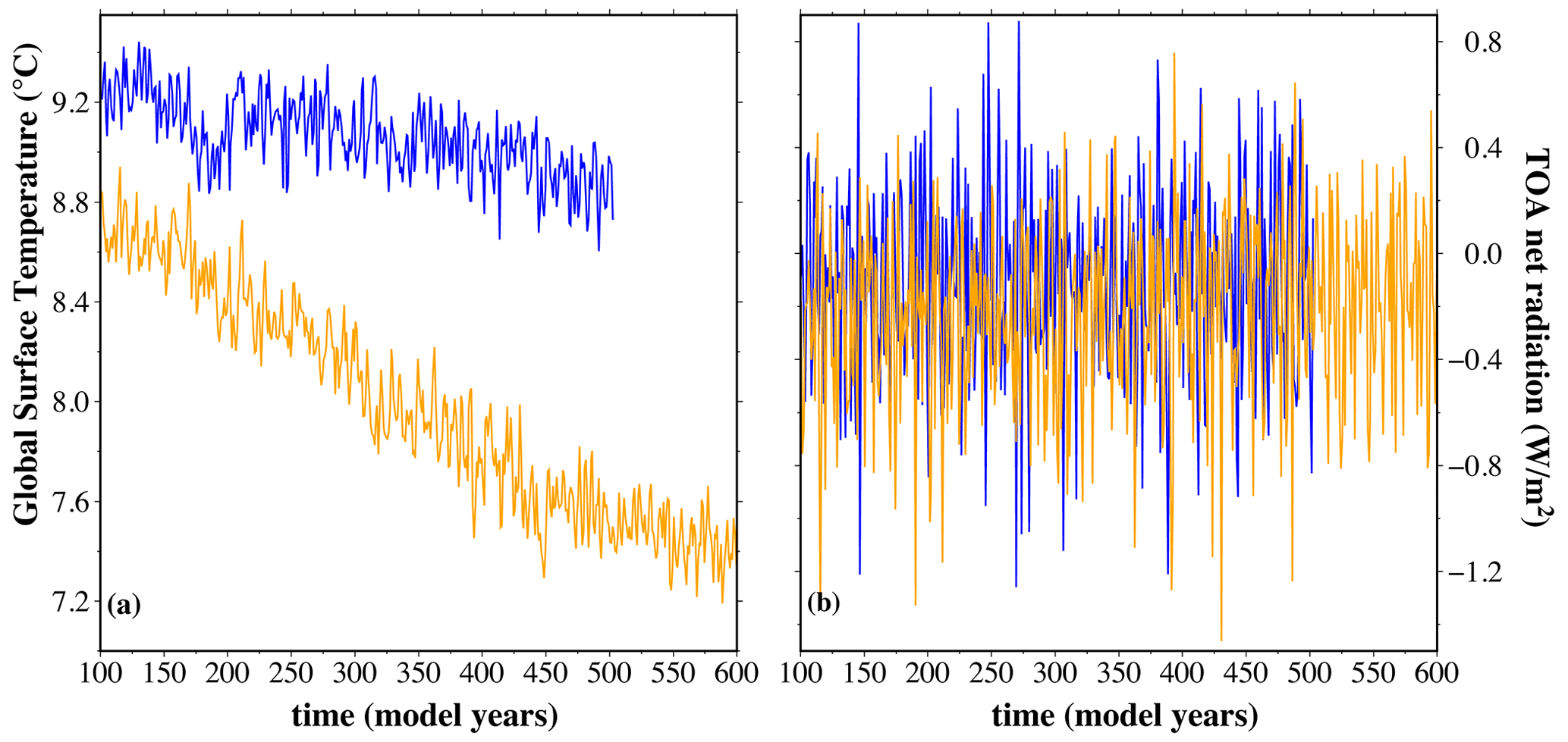
Figure C1 Panel (a) shows global near-surface temperature (in ^∘C) from LG-21 ka (blue line) and LG-26 ka (orange line). Panel (b) shows top of the atmosphere (TOA) net radiation (in W m⁻²) for LG-21 ka (blue line) and LG-26 ka (orange line).

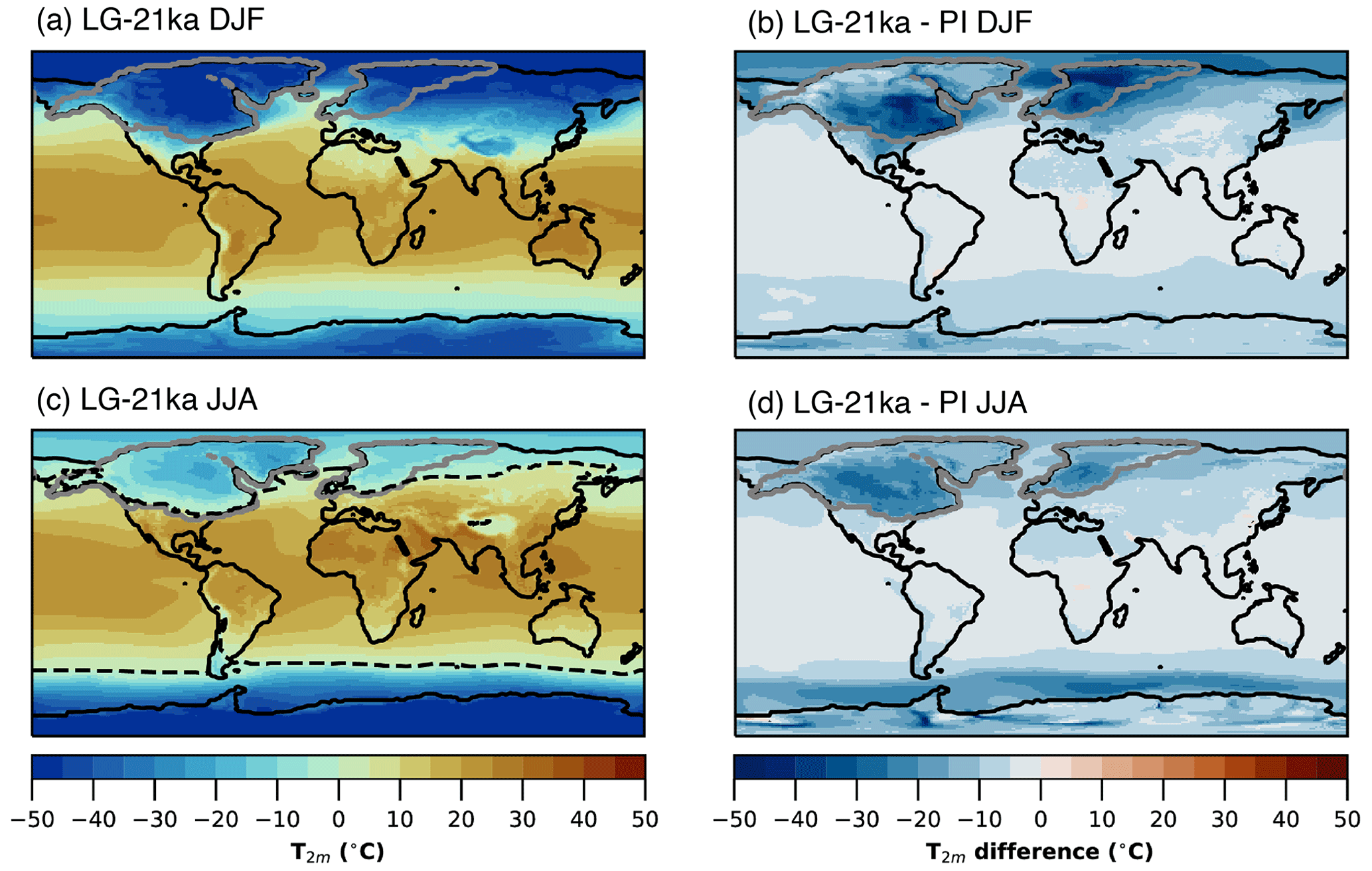
Figure C2 Near-surface temperature: (a) and (b) show DJF, while (c) and (d) show JJA, all in ^∘C. The left column shows values from the LG-21 ka simulation, while the right column shows the differences between LG-21 ka and the PI simulations. The grey contour encloses glaciated areas (>50 % ice cover). The dashed black line in (c) follows the 0 ^∘C isotherms.

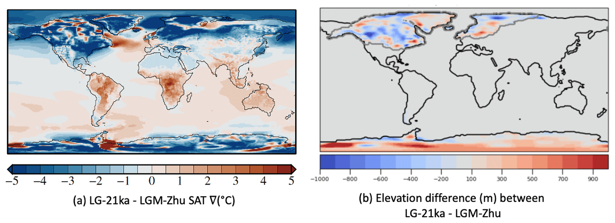
Figure C3 Panel (a) shows the difference in the annual mean (20 years) near-surface temperature (SAT) between LG-21 ka and LGM-Zhu. Panel (b) shows the elevation difference (in metres) in CAM (1^∘ CESM grid) between LG-21 ka and LGM-Zhu. There is an approximate relationship between the colder regions (blue) in (a) and the higher elevations in (b).

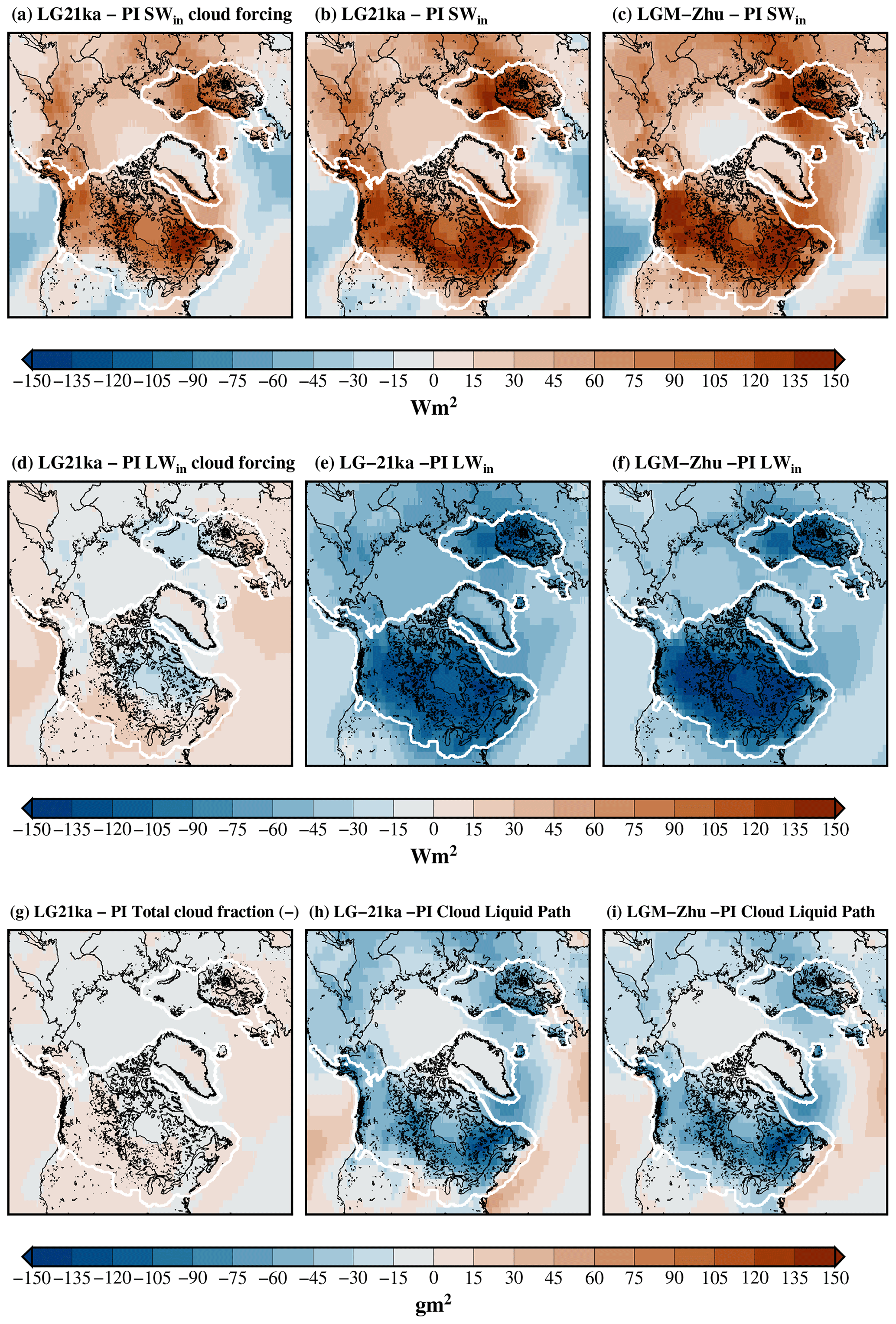
Figure C4 June–July–August anomalies (relative to the PI) for (a) LG-21 ka SW_in cloud forcing, (b) LG-21 ka SW_in, (c) LGM-Zhu (SW_in), (d) LG-21 ka LW_in cloud forcing, (e) LG-21 ka LW_in, (f) LGM-Zhu LW_in, (g) LG-21 ka total cloud fraction (–), (h) LG-21 ka cloud liquid path, and (i) LGM-Zhu cloud liquid path.

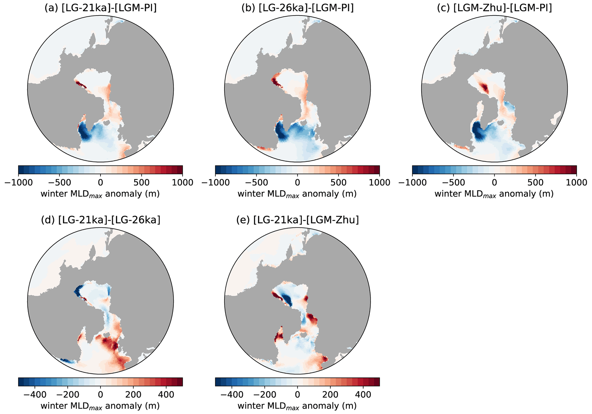
Figure C5 Anomaly of the local maximum of the mixed layer depth during winter (in metres) for (a) LG-21 ka, (b) LG-26 ka, and (c) LGM-Zhu with respect to the LGM-PI simulation and for LG-21 ka with respect to (d) LG-26 ka and (e) LGM-Zhu.

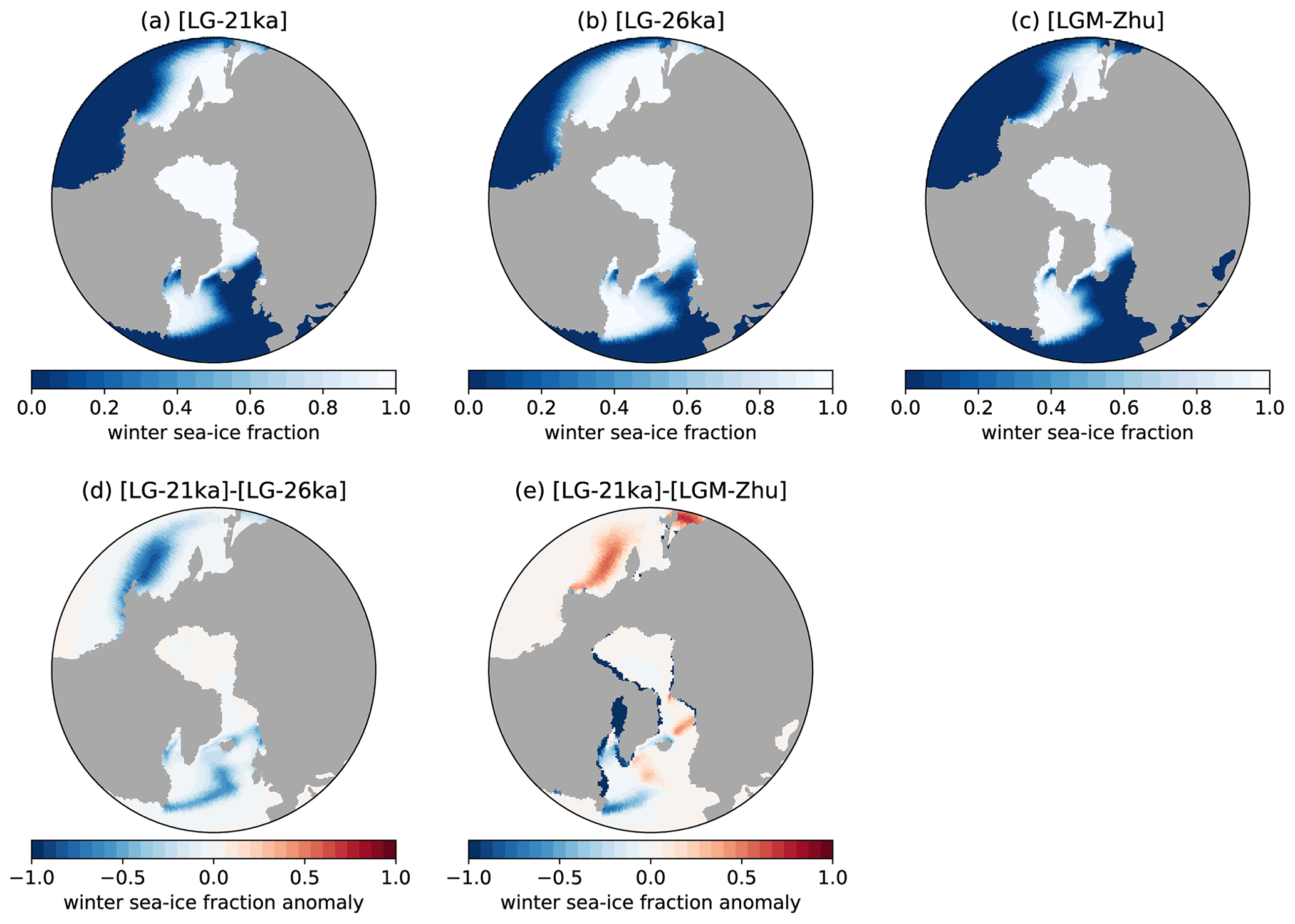
Figure C6 Sea ice fraction during winter for (a) LG-21 ka, (b) LG-26 ka, and (c) LGM-Zhu. Winter sea ice fraction anomaly for LG-21 ka with respect to (d) LG-26 ka and (e) LGM-Zhu.