New estimates of sulfate diffusion rates in the EPICA Dome C ice core

To extract climatically relevant chemical signals from the deepest, oldest Antarctic ice, we must first investigate the degree to which chemical ions diffuse within solid ice. Volcanic sulfate peaks are an ideal target for such an investigation because they are high-amplitude, short-duration (∼3 years) events with a quasi-uniform structure. Here we present an analysis of the EPICA Dome C sulfate record over the last 450 kyr. We identify volcanic peaks and isolate them from the non-sea-salt sulfate background to reveal the effects of diffusion: amplitude damping and broadening of peaks in the time domain with increasing depth and age. Sulfate peak shape is also altered by the thinning of ice layers with depth that results from ice flow. Both processes must be simulated to derive effective diffusion rates. This is achieved by running a forward model to diffuse idealised sulfate peaks at different rates while also accounting for ice thinning. Our simulations suggest a median effective diffusion rate of sulfate ions of $\mathrm{2.4}\pm \mathrm{1.7}\times {\mathrm{10}}^{-\mathrm{7}}$ m² yr⁻¹ in Holocene ice, slightly faster than suggested by previous work. The effective diffusion rate observed in deeper ice is significantly lower, and Holocene ice shows the highest rate of the last 450 kyr. Beyond the Holocene, there is no systematic difference between the effective diffusion rates of glacial and interglacial periods despite variations in soluble ion concentrations, dust loading, and ice grain radii. Effective diffusion rates for 40 to 200 ka are relatively constant and of the order $\mathrm{1}\times {\mathrm{10}}^{-\mathrm{8}}$ m² yr⁻¹. Our results suggest that the diffusion of sulfate ions within volcanic peaks is relatively fast initially, perhaps through an interconnected vein network, but slows significantly after 40 kyr. In the absence of clear evidence for a controlling influence of temperature on sulfate diffusivity with depth and age, we hypothesise that the rapid decrease in effective diffusion rate from the time of deposition to ice of 50 ka age may be due to a switch in the mechanism of diffusion resulting from the changing location of sulfate ions within the ice microstructure and/or interconnectedness of veins and grain boundaries.

1 Introduction

Records of chemical impurities within ice cores are frequently used as climate proxies (e.g. Wolff et al., 2010) or utilised in ice core dating via the identification of seasonal fluctuations (e.g. Sigl et al., 2016) or deposition from volcanic eruptions (Sigl et al., 2013). The assumption that chemical impurity signals have not undergone significant post-depositional alteration is typically implicit in these applications. However, we know that post-depositional alteration of the chemical properties of ice does take place and that this can become increasingly important as older, deeper ice is considered.

In this study we focus on one post-depositional process, the diffusion of chemical ions driven by concentration gradients within the ice structure. As we will explore, the strongest evidence for the diffusion of chemical signals in ice cores is seen in sulfate records. Volcanic sulfate peaks located in deep, old ice are typically lower in amplitude and span a wider age range relative to their recently deposited counterparts (Fig. 1). Barnes et al. (2003a) quantified the diffusion rates of sulfate and chloride ions in the Holocene ice of the Antarctic EPICA Dome C (EDC) core as $\mathrm{3.9}\times {\mathrm{10}}^{-\mathrm{8}}$ and $\mathrm{2.0}\times {\mathrm{10}}^{-\mathrm{7}}$ m² yr⁻¹, respectively. We note that an incorrect value for sulfate ($\mathrm{4.7}\times {\mathrm{10}}^{-\mathrm{8}}$ m² yr⁻¹) was quoted in the abstract of their study. Please see their Sect. 2.3 for their results. Two mechanisms enabling solute diffusion along veins or grain boundaries were proposed, both linked to processes related to ice grain growth that promote connections between veins. Here we consider ice grains to be surrounded by grain boundaries that intersect at triple junctions, which are populated by veins (see Fig. 2e of Ng, 2021). Soluble ionic impurities tend to be concentrated along grain boundaries and within veins (Barnes et al., 2003b; Bohleber et al., 2021; Mulvaney et al., 1988), where liquids can exist at temperatures below zero. The eutectic temperature of sulfuric acid (the origin of the majority of sulfate within polar ice) is −73 °C, which is well below the coldest ice sheet temperatures on Earth, meaning sulfate ions are likely to be mobile.

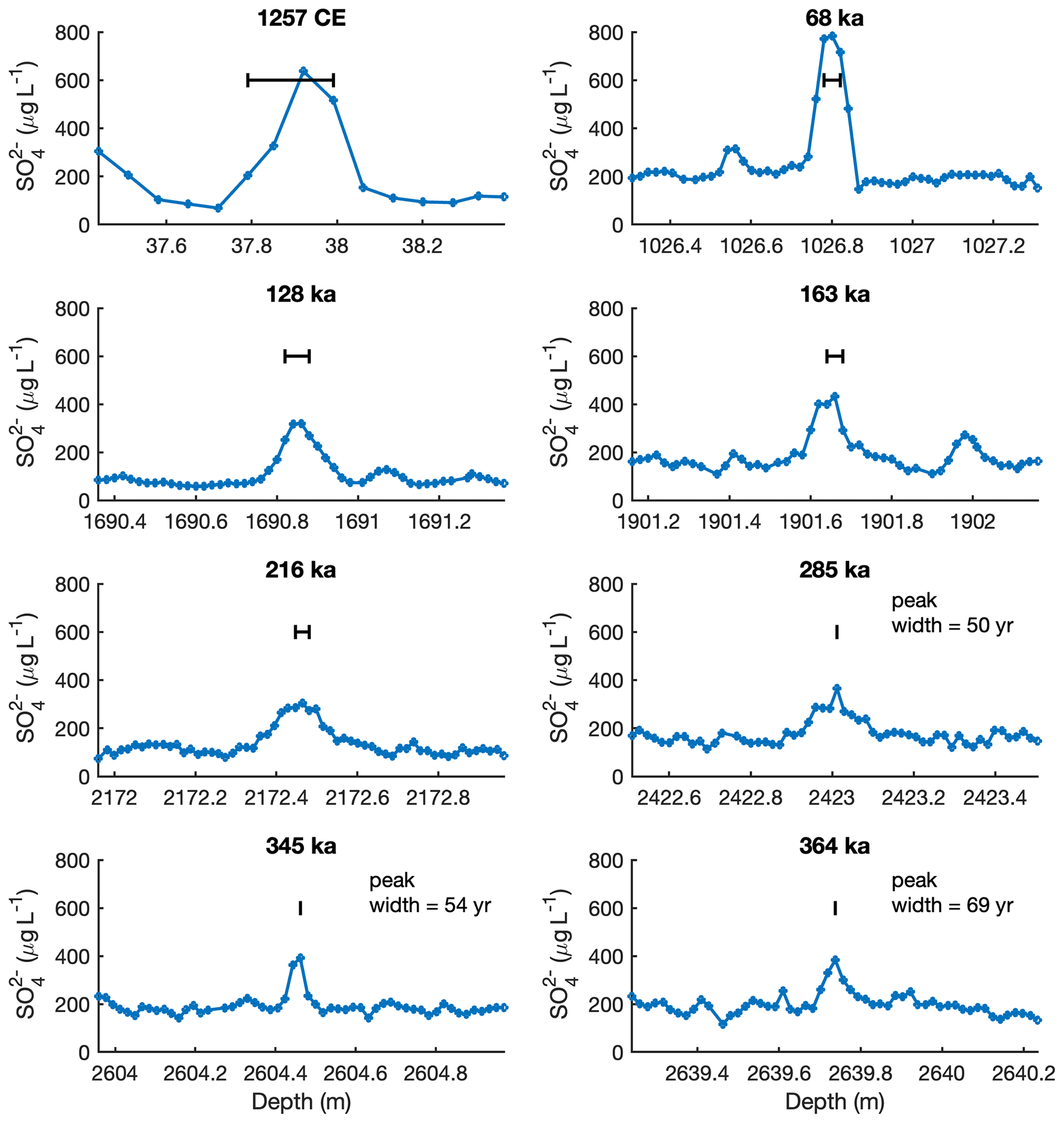
Figure 1 Selected volcanic sulfate peaks in the EDC ice core showing changes in peak shape with depth. All peaks shown have a total sulfate flux of 63.7–91.0 mg m⁻² and in each case the x axis spans a depth range of 1 m and the y axis has the same scaling. The horizontal black bar on each plot indicates the depth range equivalent to 5 years of accumulation at that depth in the core.

In a high-profile study, Rempel et al. (2001) argued that “anomalous diffusion” of chemical ions along temperature gradients can occur within veins, resulting in the vertical advection of chemical signals within the ice sheet while maintaining similar amplitudes. The implication was that a an Eemian age chemical signal in the GRIP ice core could be displaced by as much as 50 cm depth relative to its location at deposition. Such a process would have consequences for cross-matching events, such as volcanic eruptions, between ice cores for stratigraphic purposes. Ng (2021) revisited this hypothesis and challenged the impact of this phenomenon by noting that since soluble impurity loading does not appear to control ice grain size (Durand et al., 2006), and by extension ice vein density, the Gibbs–Thomson effect (related to surface energy) should cause vein radii to change by producing solute concentration gradients that diminish bulk concentration anomalies. Ng argued that chemical ions present in the veins (grain boundaries and grain interiors are not considered) quickly diffuse as a result so that peaks will be damped and broaden. For the ice core community, Ng's revision means that chemical signals present in the veins will not be displaced in age and depth, but they will be destroyed over time, provided they are free to diffuse unimpeded through interconnected veins towards low-solute-concentration regions.

In the context of international projects such as the Beyond EPICA Oldest Ice Core (BE-OIC), which aims to recover an Antarctic ice core dating back 1.5 Myr (Lilien et al., 2021), it is critical to further quantify the rate at which chemical diffusion occurs in order to predict the fidelity of signal preservation at depth. Further constraints on the rates of chemical diffusion could be crucial to understanding the mechanism(s) of chemical diffusion in polar ice. However, we highlight up front that our current chemical measurement methods for ice provide only bulk chemical concentrations and do not allow us to partition ions by location within the ice structure, i.e. within grain boundaries, veins, or grain interiors. New sub-millimetre-scale measurement techniques will undoubtedly help in the future (Bohleber et al., 2021).

In this paper, we analyse volcanic sulfate signals in the EDC ice core (EPICA community members, 2004) and quantify time-dependent effective diffusion rates. This work extends the time interval considered by Barnes et al. (2003a) to well beyond the Holocene, incorporating four glacial–interglacial cycles. In order to quantify diffusion rates, we also simulate the impact of ice thinning resulting from ice flow on the preservation of chemical signals. Our work complements the recent study of Fudge et al. (2024), who used the same sulfate dataset but applied a different method to estimate effective diffusion rates. Our results are compared in Sect. 5.

2 Volcanic sulfate peaks in the EDC ice core

Individual volcanic eruptions deposit sulfuric acid on ice sheets, forming sharp, distinct peaks in sulfate profiles lasting only a few years. Volcanic sulfate peaks are many times greater in magnitude than the sulfate background, which is dominated by marine sources. Furthermore, these easily identifiable signals occur regularly through time (Wolff et al., 2023), meaning that the evolution of their form resulting from diffusion and ice thinning can be traced down-core. In this study, we use EDC sulfate data measured using fast ion chromatography (FIC) (Severi et al., 2015; Fudge and Severi, 2023).

We quantify the rate of sulfate diffusion by comparing the shape of older volcanic peaks to their likely shape shortly after deposition. This is possible because major volcanic sulfate peaks in ice cores have a well-understood, reproducible peak shape shortly after deposition (within a few hundred years). Specifically, volcanic sulfate peaks have a reproducible duration (peak width) and a Gaussian form. Following a major eruption, the aerosol loading of the stratosphere increases rapidly to a maximum a few months after a major volcanic eruption (Thomason et al., 2018) and decreases to background levels over a period of about 5 years, with an e-folding time of between 6 months and 1 year depending on the height, latitude, and magnitude of the eruption (Marshall et al., 2019). Modelling of the deposition of material on the Antarctic ice sheet from the large 1815 CE Tambora eruption suggests that deposition should occur over 3–4 years (Marshall et al., 2018). Data from ice cores from regions of high snowfall, such as WAIS Divide in Antarctica, agree with these observations and model predictions of deposition duration. Sulfate signals associated with the largest eruptions of the last millennium last for about 3 years (Koffman et al., 2013; Sigl et al., 2013). In the EDC ice core, volcanic peaks within the firn seem to be slightly wider (in terms of time) than those at WAIS Divide. The peaks for the 1257 CE eruption (unknown volcano, Fig. 1) and for Tambora (1815 CE, not shown) have peak widths between 8 and 9 years. This slightly extended width of the peak at EDC might result from a combination of mixing of snow from different layers due to snowdrift and surface roughness, the latter of which is significant compared to the low snow accumulation rate. The Gaussian form of sulfate peaks in ice cores (as opposed to the skewed distribution in the stratosphere) likely reflects a rapid process of sulfate movement occurring soon after deposition that could be investigated further.

Barnes et al. (2003a) already observed that volcanic sulfate peaks broaden (in terms of time) as they age and deepen through the Holocene in the EDC ice core. Here we extend our observations back to 450 ka. Figure 1 shows EDC volcanic sulfate peaks with a similar (within 30 %) deposition flux to the value calculated for the 1257 CE eruption (84 mg m⁻²), which implies that their initial shapes at deposition would have been similar. While Fig. 1 shows only a few examples, it is clear that the sulfate peaks decrease in amplitude and broaden (in terms of age range spanned) beyond the Holocene. The peak width estimated as <10 years for the 1257 CE eruption is approximately 17 years by 68 ka and almost 70 years at 364 ka. These observations confirm that some form of chemical diffusion occurs at EDC, causing the sulfate peaks to be spread over greater equivalent time as the core ages.

We note that during glacial periods, when the snow accumulation rate is low relative to interglacial periods, a sulfate peak with a 3-year duration would have covered a smaller depth range at deposition, and the sulfate peak height for the same-magnitude volcanic event would have been higher: assuming dry deposition dominates, the same amount of sulfate would have been deposited across a narrower depth range due to the a smaller mass of snow. We also note that the 1257 CE eruption peak is in relatively low-density firn, and therefore its ice-equivalent depth range would be about 63 % of the snow depth shown.

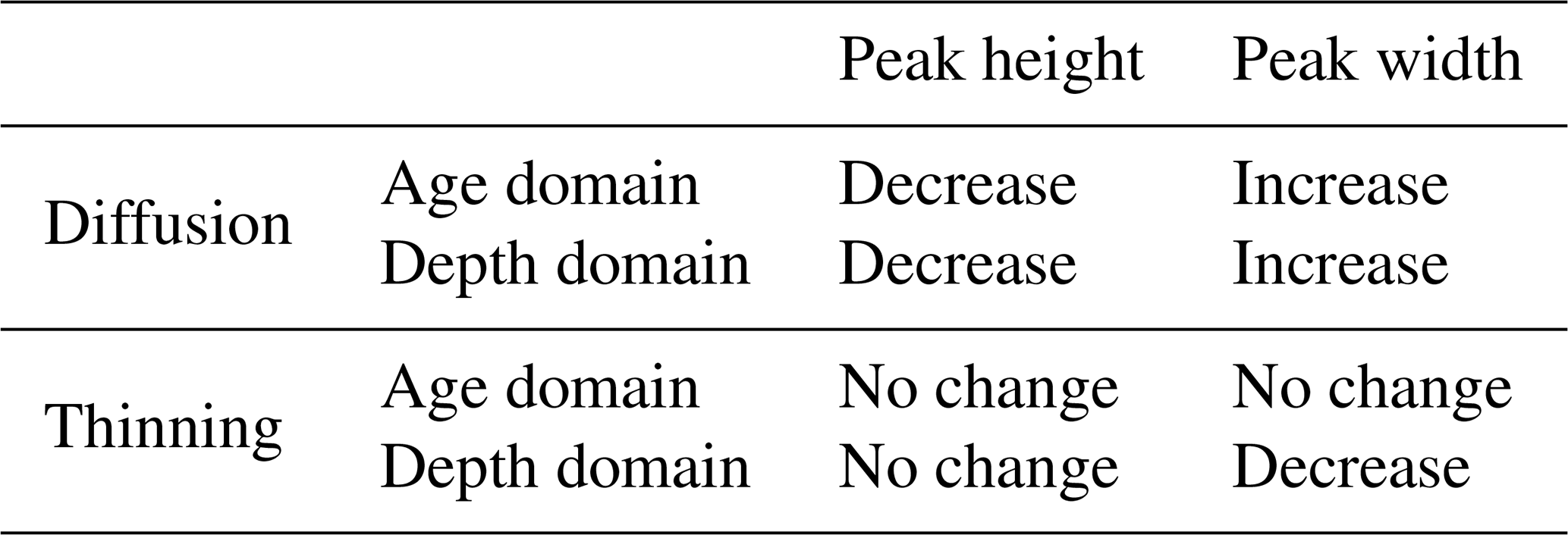
Figure 1 also illustrates the impact of ice thinning. Although the sulfate ions in older peaks have clearly diffused, damping and broadening those peaks with respect to age, the width of the sulfate peaks in terms of depth is not altered much with depth and age in the EDC core (all the x axes in Fig. 1 span 1 m). Typically, the peaks cover a depth range of about 20 cm of ice. Ice thinning narrows the depth range spanned by an individual chemical peak. However, it appears that at EDC, the combined action of peak broadening through chemical diffusion and peak narrowing via ice thinning results in a relatively constant peak width in the depth domain for the first 200 kyr. At other ice core sites, with different age–depth relationships and thinning functions, the evolution of peak shape with depth will likely be different.

The evolution of volcanic sulfate peak shapes with depth therefore represents a convolution of the impacts of both the diffusion of sulfate signals along concentration gradients and the thinning of the ice sheet in which a volcanic sulfate signal is hosted (Table 1).

Table 1 Summary of the impacts of diffusion and thinning on peak shape.

3 Methodology

Our aim is to constrain the effective diffusion rate of sulfate over time in the EDC core by modelling the evolution of volcanic sulfate peak shapes with depth and age, accounting for the impacts of both chemical diffusion and ice thinning. To achieve this, we first identified the volcanic peaks present in the EDC core, then generated equivalent unthinned, undiffused “input” or “deposited” peaks assuming a Gaussian form. These peaks were fed into a forward model, which simultaneously diffused them using a range of diffusion rates and thinned them according to a simple ice flow model. Comparison of each modelled (diffused and thinned) peak with the peak preserved in the ice core (also diffused and thinned) allowed the optimum diffusion rate to be selected for each peak. Figure 2a displays a flowchart of our methodology, which we describe in more detail in the following sections, and Fig. 2b illustrates some of the key parameters involved.

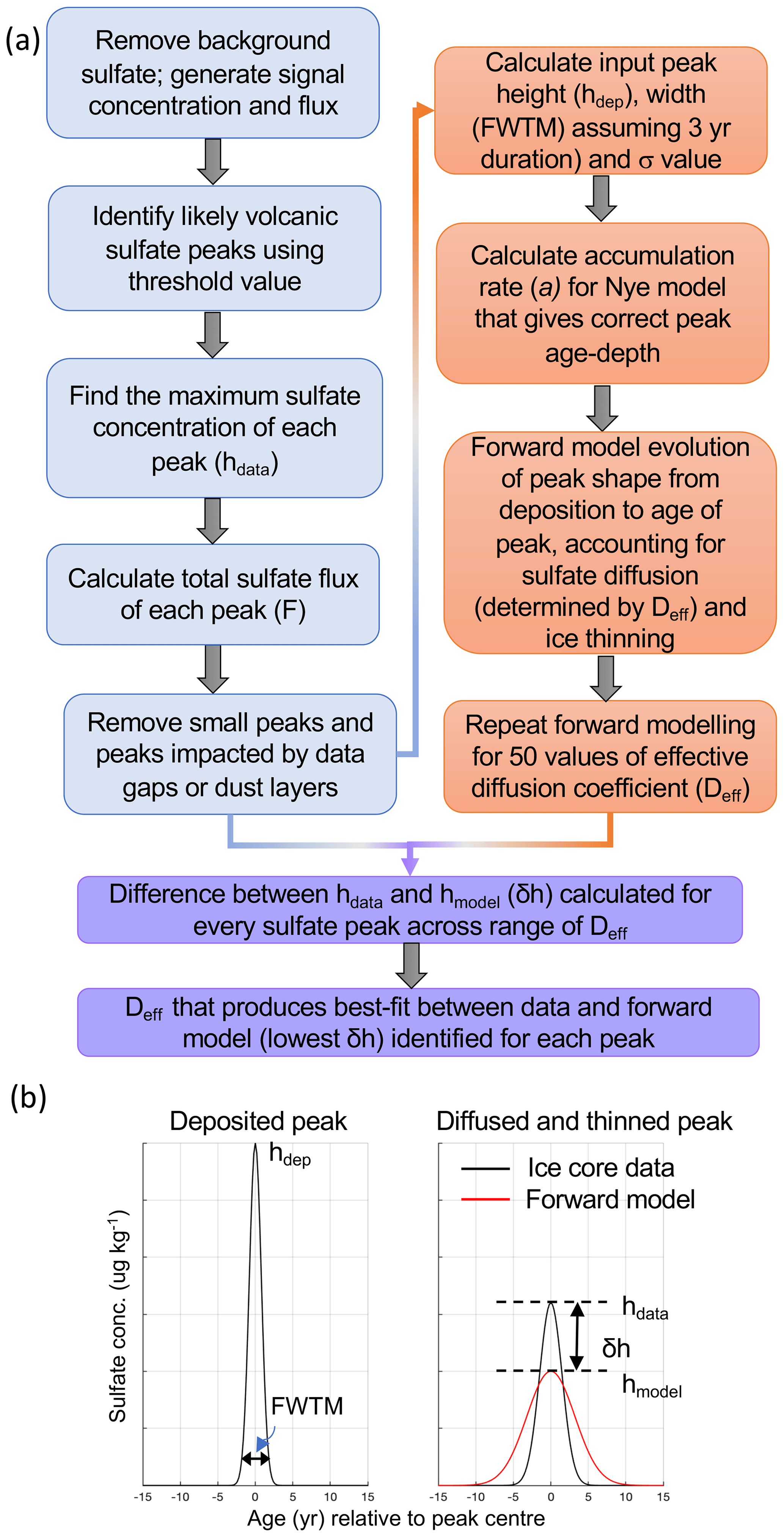
Figure 2 Illustration of the methodology. (a) Flowchart of the methodology involving analysis of EDC sulfate data (blue boxes), generation of equivalent deposited peaks and forward modelling (orange boxes), and data–model comparison to find the effective diffusion coefficient (purple boxes). (b) Example of a sulfate peak preserved in the ice core (right-hand side, black curve), its equivalent deposited peak (left-hand side), and a peak produced by the forward model (right-hand side, red curve). In this example, the forward model produces a peak that is lower in amplitude and broader than the ice core data peak, suggesting that the effective diffusion coefficient used was too high. Key parameters defined in the text are labelled.

3.1 Identification of volcanic sulfate peaks

The EDC sulfate concentration data measured by FIC have a typical resolution of 5–6 cm in the top 100 m, 3–5 cm in the interval to 770 m, and 2 cm from there to the base of the core. The long-term background signal was removed from the sulfate data by subtracting a 200-year moving median. Following Wolff et al. (2023), we multiply the residual sulfate concentrations between 0 and 358.6 m by ($\mathrm{1}/\mathrm{0.7}$) to account for a calibration discrepancy identified between FIC and standard ion chromatography measurements on EDC ice. Note that although this adjustment will impact our quantification of peak height and peak area in this depth interval, there is no impact on the estimation of diffusion rate. To calculate the annual flux (AF, µg m⁻² yr⁻¹) of sulfate we multiplied the residual sulfate concentrations (C, µg kg⁻¹) by the accumulation rate (a, kg m⁻² yr⁻¹; values from Bazin et al., 2013):

$$\begin{array}{}\text{(1)}& AF=C\times a.\end{array}$$

To identify high-amplitude volcanic peaks in the residual concentration data, we used a peak-finding algorithm (MATLAB version 2020b findpeaks) with a peak height threshold linked to the level of background variability in each 10 kyr time bin and a minimum time interval between adjacent peaks of 30 years. For each volcanic sulfate peak identified and retained, we calculated the total sulfate flux (F) by integrating the flux data with respect to time between the peak edges set by local minima in the background data. All sulfate peaks with a total flux <25 mg m⁻² were discarded (1027 out of 1618 events removed) to avoid using small peaks that may result from background signal variability and to limit the bias towards larger-magnitude events with depth. This sulfate flux is just under half the magnitude of the Tambora 1817 CE eruption in the EDC record. Identification of enough volcanic peaks for reliable analysis became difficult at > 450 ka.

Traversi et al. (2009) identified anomalous narrow, high-amplitude sulfate peaks in the EDC record, speculated to result from the migration of sulfate into specific horizons within the ice. Each of these peaks is bordered by regions of relative sulfate depletion, hence the hypothesis that sulfate has moved, or even been “sucked”, into the peak horizon (see Fig. 3 of Wolff et al., 2023). Although Traversi et al. (2009) found that these peaks first appeared beyond 2800 m depth (∼450 ka), we found some similar peaks during our analysis of shallower and/or younger ice. These caused a problem for our analysis because they were identified as volcanic events by our peak-finding code but clearly did not result from a diffused volcanic peak. In order to objectively identify these anomalous peaks, we took advantage of the fact that they tend to be associated with sharp, high spikes in dust content. All sulfate peaks below 2100 m (204 ka) were checked for an anomalously high dust peak at the same depth. If a coincident dust peak was found, then that sulfate peak was removed from analysis (43 in total).

Lastly, we removed any peaks that were impacted by data gaps due to missing samples. Peaks between 0 and 770 m with a data gap >14 cm and peaks between 770 m and 2800 m with a data gap >6 cm within its full-width depth interval were excluded (10 peaks). After all these filters were applied, we had 537 peaks remaining.

3.2 Generation of input peak shapes

For a Gaussian function, the full width at tenth maximum (FWTM) is given by

$$\begin{array}{}\text{(2)}& \text{FWTM}=\mathrm{4.292}\times \mathit{\sigma },\end{array}$$

where σ is the standard deviation of a Gaussian function, while the area (A) under a peak of height h is

$$\begin{array}{}\text{(3)}& A=h\times \mathit{\sigma }/\mathrm{0.3989}\end{array}$$

so that

$$\begin{array}{}\text{(4)}& A=h\times \text{FWTM}/\mathrm{1.712}.\end{array}$$

To obtain the initial deposited peak (the input to our forward model), we assume that the total sulfate flux F (equivalent to A in Eqs. 3 and 4) of the peak has not changed since deposition and that the FWTM of the initial deposited peak was 3 years (see Sect. 2). Rearrangement of Eq. (4) then gives us the peak height maximum (h) of the initial peak in units of annual flux (µg m⁻² yr⁻¹), which can be used in Eq. (1) to give us the peak height maximum of the initial peak in units of concentration (h_dep) that is an input to our forward model. The ice-equivalent depth in metres of 3-year FWTM is calculated via

$$\begin{array}{}\text{(5)}& \text{FWTM}\left(m\right)=\text{FWTM}\left(yr\right)\times a/\mathit{\rho },\end{array}$$

where ρ is ice density (917 kg m⁻³). The resulting FWTM is used to obtain σ in units of metres of ice via Eq. (2).

The duration of volcanic sulfate peak deposition may vary by a few years, potentially impacting our estimate of the effective diffusion coefficient. For this reason, all peaks younger than 60 ka were additionally run through the forward model with input peak widths (FWTMs) equivalent to 1 and 5 years. Preliminary testing showed that the choice of input peak width had a negligible impact on the estimated effective diffusion coefficient for older peaks.

3.3 Forward model of chemical diffusion and ice thinning

We modelled the change in concentration of sulfate ions (C) with time (t) along ice depth (z) as ions diffuse along a concentration gradient according to Fick's second law,

$$\begin{array}{}\text{(6)}& {\displaystyle \frac{\partial C}{\partial t}}=D_{\mathrm{eff}}{\displaystyle \frac{{\partial }^{\mathrm{2}}C}{\partial z^{\mathrm{2}}}},\end{array}$$

where D_eff is the effective diffusion coefficient in units of m² yr⁻¹ and z is defined as height in metres above the ice sheet bed. We can treat sulfate diffusion in the ice sheet as a 1D (as opposed to 3D) problem by assuming that the sulfate concentration is constant across any given horizontal layer of the ice sheet. In our forward model the effective diffusion rate for each iteration is constant with time and an additional term is introduced to the diffusion equation to describe the change in sulfate concentration over time due to ice thinning:

$$\begin{array}{}\text{(7)}& {\displaystyle \frac{DC}{Dt}}={\displaystyle \frac{\partial }{\partial z}}\left(D_{\mathrm{eff}}.{\displaystyle \frac{\partial C}{\partial z}}\right)+v\left(z\right){\displaystyle \frac{\partial C}{\partial z}}.\end{array}$$

Here vertical velocity (v) is estimated using a simple Nye model of ice flow (Nye, 1963). As the EDC core was drilled close to the ice divide, ice flows radially from the site (Legresy et al., 2000), meaning the ice sheet dynamics can also be represented by a 1D model (Parrenin et al., 2007). The Nye model predicts that the layer thickness (λ, m of ice) equals the layer thickness at deposition on the surface (λ₀, m of ice) and is zero at the bed, changing linearly in between; i.e. the thinning rate is constant with depth, as follows:

$$\begin{array}{}\text{(8)}& {\displaystyle \frac{\mathit{\lambda }}{{\mathit{\lambda }}_{\mathrm{0}}}}={\displaystyle \frac{z}{H}},\end{array}$$

where H is the ice sheet thickness. The Nye model uses ice-equivalent length and depth units to avoid including snow and firn compaction in the calculation of strain rate and assumes that there is no melting at the bed. Nye (1963) therefore assumes that the vertical strain rate (${\dot{\mathit{\epsilon }}}_{zz}$) is uniform at any given instant, as follows:

$$\begin{array}{}\text{(9)}& {\dot{\mathit{\epsilon }}}_{zz}=-{\displaystyle \frac{a_{\mathrm{ice}}}{H}},\end{array}$$

where a_ice is the accumulation rate in units of m ice yr⁻¹. To obtain vertical velocity (v) at height z, the vertical strain rate is integrated from the base of the ice sheet (where v=0 in all directions) to height z:

$$\begin{array}{}\text{(10)}& v\left(z\right)={\int }_{\mathrm{0}}^z{\dot{\mathit{\epsilon }}}_{zz}\mathrm{d}z={\int }_{\mathrm{0}}^z-{\displaystyle \frac{a_{\mathrm{ice}}}{H}}\mathrm{d}z=-{\displaystyle \frac{a_{\mathrm{ice}}z}{H}}.\end{array}$$

For numerical convenience, the Eulerian depth coordinate z of Eqs. (6)–(10) is replaced with Lagrangian coordinate x in our model. x=0 at the maximum value of C in the centre of the sulfate peak and x increases towards the ice surface. With this coordinate change, the relative velocity of ice at any distance x relative to the centre of a sulfate peak is simply given by

$$\begin{array}{}\text{(11)}& v\left(x\right)=-{\displaystyle \frac{a_{\mathrm{ice}}x}{H}}.\end{array}$$

The Nye model was effectively tuned to the AICC2012 chronology (Bazin et al., 2013) by calculating the value of a_ice for the height above the bed (z) and age (t) of each sulfate peak:

$$\begin{array}{}\text{(12)}& a_{\mathrm{ice}}=-{\displaystyle \frac{H}{t}}ln{\displaystyle \frac{z}{H}}.\end{array}$$

In our calculations, H was kept constant at 3165 m, which is the mean ice sheet thickness over the time interval considered here at EDC according to Parrenin et al. (2007). The more complex Lliboutry model used by Parrenin et al. (2007) is certainly a more precise description of thinning, but a tuned Nye model mimics it closely in the top two-thirds of the ice sheet (where thinning is close to linear), and its use is justified by the considerable reduction in computational complexity for this problem.

For each sulfate peak, h_dep and σ of the initial deposited peak were used to generate a Gaussian distribution of sulfate concentration along length x, which was then diffused and thinned to age (t) via Eq. (7), solved using a partial differential equation solver (MATLAB version 2020b pdepe). The spatial resolution of x is higher than 1 cm for each metre either side of the peak centre. This forward model can be run at regular time intervals to produce a 3D representation of sulfate peak evolution through time and space (Fig. S1).

3.4 Identification of effective diffusion rates

For each volcanic peak identified in the data, the forward model was run using 50 effective diffusion rates log-spaced between 10⁻⁹ and 10⁻⁶ m² yr⁻¹. As described above (Sect. 3.2), peaks <60 ka were run for three different values of input peak duration (1-, 3-, and 5-year FWTM). For each individual simulation, the difference (δh; Fig. 2b) between the modelled maximum peak height sulfate concentration (h_model) and the peak height of the selected sulfate concentration data peak (h_data) was calculated and saved. For each volcanic event, we find the effective diffusion rate that produces the best fit between modelled peak and data peak, with the lowest value of δh.

4 Results

4.1 Effective diffusion rates of sulfate in EDC ice

Our forward modelling provides an estimate of the effective diffusion rate – that is, the time-weighted rate of diffusion over the entire history of the peak – for every volcanic event identified in the EDC sulfate record. To minimise the effect of any one peak, we have calculated the median effective diffusion rate across all peaks in each 10 or 20 kyr time bin (Fig. 3). The median absolute deviation (MAD) of the effective diffusion rate across all peaks in each time bin is calculated to provide an uncertainty envelope (vertical bars in Fig. 3). Calculating the mean and standard deviation within each time bin produces a similar result (Fig. S2). Effective diffusion rates range from $\mathrm{2.4}\times {\mathrm{10}}^{-\mathrm{7}}$ m² yr⁻¹ for 0–10 ka to $\mathrm{1.6}\times {\mathrm{10}}^{-\mathrm{9}}$ m² yr⁻¹ for 410–430 ka.

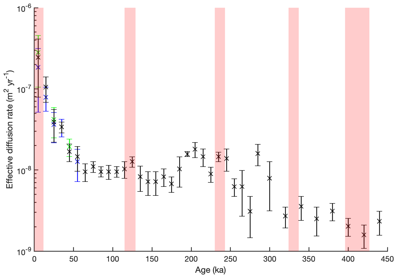
Figure 3 Effective diffusion rates of sulfate in the EDC core. For each time bin, the median (black crosses) and median absolute deviation (MAD, black vertical bars) of effective diffusion rates across all volcanic events are shown. For the first six time bins, median and MAD of effective diffusion rates are also shown for volcanic peaks with FWTM of 1 year (green) and 5 years (blue). Varying peak width has a negligible impact on results from older time bins. Time bins are 10 kyr duration except those > 300 ka, which are 20 kyr in duration. Light red shaded regions denote interglacial periods.

Our results suggest there is a significant decrease in the effective diffusion rate with age in the EDC ice core. Median rates are fastest in Holocene ice ($\mathrm{2.4}\times {\mathrm{10}}^{-\mathrm{7}}$ m² yr⁻¹) and decrease sharply to $\mathrm{1.7}\times {\mathrm{10}}^{-\mathrm{8}}$ m² yr⁻¹ by 40–50 ka. Effective diffusion rates are significantly higher in the first 40 kyr of the EDC record relative to the remaining time. From 50 ka onwards, diffusion rates are an order of magnitude lower than in the Holocene, remaining consistently around $\mathrm{1.0}\pm \mathrm{0.3}\times {\mathrm{10}}^{-\mathrm{8}}$ m² yr⁻¹ until 200 ka.

Between 200 and 240 ka, the median effective diffusion rates appear to increase slightly, up to $\mathrm{1.8}\times {\mathrm{10}}^{-\mathrm{8}}$ m² yr⁻¹. This would imply that diffusion rates in ice of this age are higher than in younger ice, which would surely require a concurrent change in a controlling variable such as in temperature, chemistry, or ice microstructure. This possibility will be explored in Sect. 5.1. The overall trend from 240 to 450 ka is negative, implying that effective diffusion rates are reduced with age and depth. However, the relatively high spread of D_eff values and subsequent high MAD values for several time bins, relative to the younger portion of the core (Fig. 5), make it difficult to have high confidence in this feature.

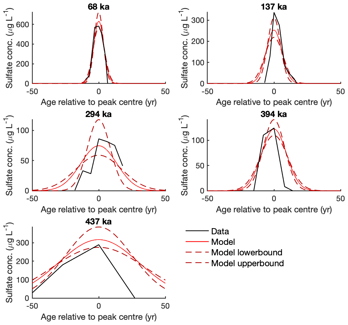
Figure 4 Comparison of sulfate peaks in the ice core with peaks produced by the forward model. EDC sulfate peaks (black) of different age (indicated by bold titles) are compared to forward model simulations (red) produced using the median effective diffusion rate for the 10 kyr time bin (or 20 kyr time bin if peak age >300 ka). Model upper and lower bounds (dashed dark red) are products of the median ± MAD effective diffusion rate (as Fig. 3).

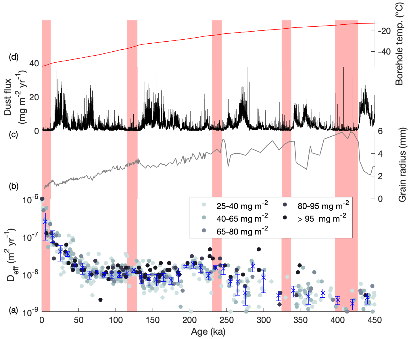
Figure 5 Effective diffusion rate estimated for each EDC volcanic sulfate peak compared to grain size and dust loading. (a) Effective diffusion coefficient (D_eff) estimated for each individual volcanic sulfate peak, colour-coded according to the magnitude of total sulfate flux (see legend). Median D_eff values and MAD range for each time bin are also plotted (blue crosses and vertical bars, as Fig. 3). (b) EDC grain radius (EPICA community members, 2004). (c) EDC dust flux (Lambert et al., 2008). (d) EDC borehole temperature profile (Buizert et al., 2021). Light red shaded regions denote interglacial periods.

Broadly speaking then, effective diffusive rates are relatively fast in the Holocene and into the last glacial period but then appear to stabilise or possibly continue to decrease at a much-reduced rate back in time. If we consider again that these rates are the product of the evolution of the diffusion rate over time and assuming that all peaks are subjected to higher rates of diffusion in the first 40 kyr of their history, the actual rate of diffusion occurring in older portions of the core must be considerably lower than displayed in Fig. 3. A stabilisation or plateau in effective diffusion rate does not mean that zero diffusion is occurring in ice of that age. It indicates that the diffusion rate has not changed since the last time window.

Looking only at our time-binned effective diffusion rates, there is no apparent systematic difference between ice deposited in a glacial period versus an interglacial period (Fig. 3, red shading indicates interglacials). Excluding the 0–45 ka time interval, the median effective diffusion rate for all the sulfate peaks in glacial periods is $\mathrm{8}\pm \mathrm{4}\times {\mathrm{10}}^{-\mathrm{9}}$ m² yr⁻¹(± MAD). The median value is slightly higher for interglacial periods at $\mathrm{1.1}\pm \mathrm{0.4}\times {\mathrm{10}}^{-\mathrm{8}}$ m² yr⁻¹(± MAD) but the MAD envelopes overlap, meaning there is no significant difference between the two.

4.2 Model validation

Before further interpretation of our results, we validate our forward modelling approach by testing if the model can simulate sulfate peaks similar to those in the EDC record using the effective diffusion rates calculated for the enclosing time bin (Fig. 4). The model performs well for the sulfate peaks shown at 68, 294, 394, and 437 ka. The range of peak heights simulated by the model (between the upper and lower bounds) includes the height of the sulfate peak in the ice core. For the 137 ka peak, the model appears to slightly overestimate the rate of sulfate diffusion that has occurred. However, the mismatch is slight, and if Fig. 4 is re-plotted using peak-specific effective diffusion rates calculated by the model (Fig. S3), the match between the model and data is excellent for every peak, as one would expect. Several of the modelled sulfate peaks, e.g. 394 ka, appear to be broader than the ice core sulfate peaks. As thinning does not impact peak width in the age domain (Table 1), this suggests that diffusion is underestimated or, more likely, that the distribution of sulfate is not strictly Gaussian.

We further validate our modelling approach by running it with effective diffusion rates derived from the literature (Sect. 5.2) to observe the different peak shapes produced with a rate of D_eff values with (Fig. S4) and without (Fig. S5) the inclusion of thinning.

5 Discussion

This study suggests that the diffusion rate of sulfate at EDC is relatively rapid in the first 40 kyr and slows down to a quasi-constant value from then onwards. Here we will discuss the various factors that could contribute to this temporal trend, compare our results to previous work, and discuss the implications of this temporal variation in diffusion rate for potential mechanisms of sulfate diffusion.

5.1 Factors potentially influencing diffusion rate

At EDC sulfate ions can be dissolved in liquid within veins and at grain boundaries because the ice sheet temperature (Fig. 5d) is always above the eutectic temperature of −73 °C for sulfuric acid (Gable et al., 1950). Although some sulfate may be present within the ice lattice at East Antarctic sites (Ohno et al., 2005), it cannot account for the majority of sulfate at EDC because, as Barnes et al. (2003a) explained, self-diffusivity within ice is much slower than the effective diffusion rates we observe. The borehole temperature at EDC increases with depth from −52 °C at the surface to −12.7 °C at 2800 m, the deepest ice considered here, due to the geothermal heat flux. As diffusion is a temperature-dependent process, we might expect effective diffusion rates to increase with depth and age in the ice core but the opposite trend is seen in our effective diffusion data. One possibility is that chemical reactions in the ice, for example the precipitation of salt as sulfuric acid reacts with dust to form the anomalous peaks discussed in Sect. 3.1 (Traversi et al., 2009), remove sulfate ions from solution. The occurrence of these anomalous peaks does appear to increase with depth and age and warrants further investigation.

Increasing temperature with depth in the ice sheet impacts the ice microstructure in which sulfate ions are present because higher temperatures promote the growth of larger ice grains via normal grain growth (Durand et al., 2009). Barnes et al. (2003a) proposed two mechanisms for sulfate diffusion that would both result in an increase in effective diffusion rate with increased grain growth rate. However, a gradual transformation from <1 mm to >5 mm grains, with no marked change in overall grain growth rate, is observed through the section of EDC core considered here (Fig. 5b). Our analysis does not extend to the region of the ice in which grain evolution is dominated by migration recrystallisation, which begins at ∼3000 m where borehole temperatures rise above −10 °C (Durand et al., 2009).

The process of normal grain growth is also thought to be impacted by impurities, in particular insoluble particles, that effectively pin the grain boundaries and limit the rate of grain growth (Durand et al., 2006). This grain boundary pinning is the reason for the sharp decreases in grain radius observed at EDC at each transition from low-dust interglacial ice to relatively high-dust glacial ice (Fig. 5b and c). Barnes et al. (2003a) speculated that the high dust concentrations of glacial periods would translate to reduced sulfate diffusivities due to the reversals in ice grain growth rate. In addition, Barnes et al. (2003a) also speculated that sulfate ions would be less soluble and therefore less mobile in glacial periods relative to interglacials because sulfuric acid would be neutralised through reaction with (carbonate-rich) dust particles. As stated in Sect. 4.1, we do not observe any significant difference between the effective diffusion rates calculated for glacial and interglacial ice, except the Holocene. Again, we highlight the 50–200 ka interval, which spans the last interglacial as well as two glacial periods either side – the D_eff values are consistently stable at around $\mathrm{1.0}\pm \mathrm{0.3}\times {\mathrm{10}}^{-\mathrm{8}}$ m² yr⁻¹.

However, something changes at >200 ka, after which more variable D_eff values are observed both over time and within time bins. Looking at the raw grain radius data (Fig. 3 of Durand et al., 2009) used to calculate the mean value shown in Fig. 5b (which is all that could be found in data repositories online), the individual grain radii are clearly more variable in this older age interval. Between 0–200 ka (∼ 0–2000 m) the interglacial–glacial contrast in grain radius is ≲0.5 mm, whereas in the 200–450 ka interval (∼ 2000–2800 m) the raw data show repeated variations on the order of 4 mm. Even if the raw grain radius data could be compared to our D_eff values, it is unlikely there would be a statistically significant relationship; however, it seems fair to suggest that this marked increase in the variability of grain growth rate with depth and age likely contributes to the increased range of D_eff values predicted for ice >200 ka.

Finally, we examine if the magnitude of the sulfate peak imparts any bias or trend in our results (Fig. 5a). There is no relationship between the total flux of sulfate and D_eff. Overall, it is difficult to attribute the variation in the EDC sulfate effective diffusion rate observed with depth and age to any of the above factors.

5.2 Comparison to published values

Our model predicts a median effective diffusion rate of $\mathrm{2.4}\pm \mathrm{1.7}\times {\mathrm{10}}^{-\mathrm{7}}$ m² yr⁻¹ in Holocene ice (0–10 ka) with values for individual events ranging from $\mathrm{1}\times {\mathrm{10}}^{-\mathrm{6}}$ to $\mathrm{5.2}\times {\mathrm{10}}^{-\mathrm{8}}$ m² yr⁻¹. The previous estimate for the effective diffusion rate of sulfate in Holocene ice at EDC is $\mathrm{3.9}\pm \mathrm{0.8}\times {\mathrm{10}}^{-\mathrm{8}}$ m² yr⁻¹ (Barnes et al., 2003a). This is significantly lower than both our median value for the 10 kyr interval and the rates implied by volcanic peaks around 10 ka only (Fig. 5): our median effective diffusion rate for 9–11 ka ice is $\mathrm{1.6}\pm \mathrm{0.5}\times {\mathrm{10}}^{-\mathrm{7}}$ m² yr⁻¹ (n=7). Fudge et al. (2016) estimated an even lower Holocene ice effective diffusivity of $\mathrm{2.2}\times {\mathrm{10}}^{-\mathrm{8}}$ m² yr⁻¹ in the WAIS Divide ice core, which is a warmer location.

Beyond the Holocene, our estimate of $\mathrm{1.0}\pm \mathrm{0.3}\times {\mathrm{10}}^{-\mathrm{8}}$ m² yr⁻¹ for 50–200 ka is higher than the new EDC estimate for 0–450 ka ice of $\mathrm{5}\pm \mathrm{2}\times {\mathrm{10}}^{-\mathrm{9}}$ m² yr⁻¹ proposed by Fudge et al. (2024) and our uncertainty ranges do not overlap. However, if our more variable estimates for effective diffusivity in >200 ka ice are included, then our median effective diffusivity for the entire 50–450 ka interval is $\mathrm{8}\pm \mathrm{4}\times {\mathrm{10}}^{-\mathrm{9}}$ m² yr⁻¹, within the range of the Fudge et al. value.

Overall, these comparisons are encouraging, both for providing confidence in our methodology and for confirming that previous estimates for sulfate diffusivity in EDC ice are not wildly different. Still, significant differences exist in the effective diffusion rate estimations of three EDC studies that utilise the same sulfate dataset but different methodologies.

Barnes et al. (2003a) not only targeted volcanic sulfate peaks in the EDC record but also performed a windowed-differencing operation on the entire Holocene sulfate time series to quantify signal damping and fit a diffusion model to the resulting trend. The higher Holocene ice D_eff produced by our method could therefore result from faster sulfate diffusion along the steep concentration gradients of volcanic peaks relative to the muted variations of background marine sulfate. This might actually be related to differences in location within the ice microstructure: in ice with a relatively low background-level sulfate concentration, sulfate may mainly be accommodated in two-grain boundaries, which may be discontinuously connected. In the highly concentrated volcanic sulfate peaks, at least initially the grain boundary or vein connectedness is more likely to be complete, leading to faster diffusion. An additional consideration is that Barnes et al. did not include the combined influence of diffusion and thinning; the sulfate record was “unthinned” for the purpose of their calculations of sulfate gradients. For the majority of the Holocene there is little thinning, but by 336 m (the deepest considered by Barnes et al.) a layer will be thinned to 93 % of its original width (Bazin et al., 2013), meaning the sulfate concentration gradient will be steepened slightly, with the potential for faster diffusion.

Fudge et al. (2024) used two methods to calculate the change in sulfate variability down-core. First, they applied the same method as Barnes et al. (2003a), which they refer to as “scaled mean gradient”, to all the sulfate data. Second, they identify major volcanic peaks to obtain the change in peak width over depth and time, then fit a 1D diffusion model (Fudge et al., 2016). Their approach differs from ours in that they do not assume anything about the magnitude of individual sulfate peaks at deposition. Instead, the difference in gradient or peak width is calculated as a mean (across all sulfate data for first method or all sulfate peaks for second method) between two time intervals, e.g. the Holocene and the last interglacial or the Last Glacial Maximum and the Penultimate Glacial Maximum. It therefore makes sense that their effective diffusivity estimates are lower than those we obtain for the relatively young (Holocene) volcanic peaks because their “starting” peaks have already undergone significant diffusion.

5.3 Implications of results for sulfate diffusion mechanism(s)

It is clear that initial rates of sulfate diffusion following deposition are fast. One possible mechanism is that the high concentrations of sulfate deposited from volcanic events are predominantly located within well-connected veins (as speculated above) and undergo Gibbs–Thomson diffusion, as modelled by Ng (2021), when first deposited. Ng predicts instantaneous diffusion rates for ions in the veins that are rapid ($\mathrm{2.1}\times {\mathrm{10}}^{-\mathrm{6}}$ m² yr⁻¹), an order of magnitude faster than the time-averaged effective diffusion rates we observe in Holocene ice. Ng's model would predict that larger-magnitude sulfate peaks should diffuse faster and this is not what we observe, although we admit that there are a limited number of events to consider in the Holocene.

Why does the diffusion rate decrease with depth and age? Perhaps Gibbs–Thomson diffusion (or other mechanism) is so efficient that the sulfate concentration gradient within the veins is quickly reduced, leaving only diffusion along two-grain boundaries; alternatively, the veins that are initially well-connected and conducive to diffusion become less so over time. The lack of bias of larger sulfate flux events towards higher diffusion rates within Holocene ice or elsewhere does imply that the diffusivity is not limited by the magnitude of the sulfate concentration gradient (as in Ng's model) but rather by the degree of connectivity within the ice microstructure.

As mentioned above, Barnes et al. (2003a) presented two different mechanisms for sulfate movement in ice, a “connected” vein or grain boundary model and a “disconnected” vein or grain boundary model. Both predicted diffusion rates of a similar order as the rates we estimate in the older (>50 ka) ice: 5–7 $\times {\mathrm{10}}^{-\mathrm{8}}$ m² yr⁻¹ for the connected model and $\mathrm{3}\times {\mathrm{10}}^{-\mathrm{8}}$ m² yr⁻¹ for the disconnected model. Without knowing more about the ice microstructure of EDC and the location of sulfate ions within it, it is difficult to favour one model over another. But both offer a viable mechanism for the slow diffusion regime and both can (according to Barnes et al., 2003a) operate in the veins or along grain boundaries.

We hypothesise that several different mechanisms of sulfate movement may operate across the depth and age range at EDC and that the predominance of one process over another is dependent on partitioning of sulfate within the ice microstructure. As such, it is the balance of rapid diffusion in the veins, potentially following Ng's Gibbs–Thomson model, when sulfate is first deposited versus slower Barnes-types diffusion options at grain boundaries that dictates the evolution of effective diffusion rate with the depth and age of the ice. Ice temperature does not appear to be a controlling factor on diffusivity of sulfate at EDC.

6 Summary

Our results suggest that if a sulfate signal deposited at EDC survives the relatively fast initial diffusion (Holocene ice median $D_{\mathrm{eff}}=\mathrm{2.4}\pm \mathrm{1.7}\times {\mathrm{10}}^{-\mathrm{7}}$ m² yr⁻¹) it will experience a much-reduced diffusion rate on the order of $\mathrm{1}\times {\mathrm{10}}^{-\mathrm{8}}$ m² yr⁻¹ (or less) from then on until at least 450 ka. The high variability in our estimates >200 ka makes it difficult to determine if the diffusion rate stays constant or continues to decline with age from 200 ka. In the absence of clear evidence for a controlling factor on sulfate diffusivity with depth and age, we hypothesise that the rapid decrease in diffusion rate from the time of deposition to ice of 50 ka age may be due to a switch in the dominant mechanism of diffusion resulting from the changing location of sulfate ions within the ice microstructure and/or change in the interconnectedness of veins and grain boundaries. Future work could explore this by building time-varying diffusion rates into the forward modelling.

Our findings need to be confirmed by analysis of high-resolution sulfate datasets from other ice cores. It will be interesting to compare the effective diffusivity profile of EDC with profiles from other cores that have similar or contrasting temperature profiles, chemical variations, and ice microstructure variations. Finally, sulfate is just one chemical ion of interest in deep ice. There is an urgent need to constrain effective diffusion rates for additional chemical ions, including Cl⁻ and Na⁺.