the Creative Commons Attribution 4.0 License.
the Creative Commons Attribution 4.0 License.
 | 12 Sep 2024
Glacial AMOC shoaling despite vigorous tidal dissipation: vertical stratification matters
Pengyang Song
Xianyao Chen
Gerrit Lohmann
During the Last Glacial Maximum (LGM), tidal dissipation was about 3-fold higher than today, which could have led to a considerable increase in vertical mixing. This increase might have enhanced the glacial Atlantic Meridional Overturning Circulation (AMOC), contradicting the shoaled AMOC indicated by paleoproxies. Here, we conduct ocean model simulations to investigate the impact of background climate conditions and tidal mixing on the AMOC during the LGM. We successfully reproduce the stratified ocean characteristics of the LGM by accurately simulating the elevated salinity of the deep sea and the rapid temperature decrease in the ocean's upper layers. Our findings indicate that the shoaled glacial AMOC is mainly due to strong glacial-ocean stratification, regardless of enhanced tidal dissipation. However, glacial tidal dissipation plays a critical role in the intensification of Antarctic Bottom Water (AABW) during the LGM. Given the critical role of the AMOC in (de-)glacial climate evolution, our results highlight the complex interactions of ocean stratification and tidal dissipation that have been neglected so far.
- Article
(8631 KB) - Full-text XML
-
Supplement
(385 KB) - BibTeX
- EndNote


The Atlantic Meridional Overturning Circulation (AMOC) transports heat over large distances and is therefore an essential component of the Earth's present and past climate systems (Ganopolski and Rahmstorf, 2001; Gordon, 1986; Rahmstorf, 1996; Stute et al., 2001). A major focus of paleoceanography involves understanding the contribution of the AMOC to glacial–interglacial climate change (Boyle and Keigwin, 1987; Broecker and Hemming, 2001; Clark et al., 2002; Knorr and Lohmann, 2003; Knorr et al., 2021).
The state of deep-water formation during the Last Glacial Maximum (LGM) has been discussed in the paleoclimate literature. Based on water mass properties, North Atlantic Deep Water (NADW) formation was shallower (Butzin et al., 2005; Curry and Oppo, 2005; Duplessy et al., 1988; Ferrari et al., 2014; Hesse et al., 2011; Lippold et al., 2012; Lund et al., 2011; Lynch-Stieglitz et al., 2007; Muglia et al., 2018; Skinner et al., 2017) but not much weaker (McManus et al., 2004; Sarnthein et al., 1994). At the same time, Antarctic Bottom Water (AABW) export from the Southern Ocean increased (Ledbetter and Johnson, 1976; Negre et al., 2010; Robinson et al., 2005). The salinity of glacial AABW may have been much greater than that observed today, leading to enhanced stratification of the glacial ocean between the upper and lower cells (Adkins et al., 2002; Bouttes et al., 2009; Francois et al., 1997; Jansen, 2017; Klockmann et al., 2016; Knorr et al., 2021; Lund et al., 2011; Stein et al., 2020; Watson and Garabato, 2006). Several modeling studies suggest a physical basis for the shoaled glacial AMOC, likely caused by changes in Southern Ocean sea ice (Baker et al., 2020; Butzin et al., 2005; Ferrari et al., 2014; Jansen and Nadeau, 2016; Marzocchi and Jansen, 2017; Nadeau et al., 2019; Sun et al., 2018, 2020; Watson et al., 2015) or terrestrial-ice input (Miller et al., 2012).
Coupled ocean–atmosphere model simulations of the LGM climate reveal a broad spectrum of results, showing considerable disagreement regarding whether the AMOC was weaker or stronger compared to present-day (PD) conditions (Kageyama et al., 2021; Knorr et al., 2021; Otto-Bliesner et al., 2007; Weber et al., 2007; Zhang et al., 2013). However, a critical factor often overlooked in these analyses is the significantly enhanced tidal dissipation that occurred during the LGM (Arbic et al., 2004b; Egbert et al., 2004; Green, 2010; Griffiths and Peltier, 2008, 2009; Wilmes and Green, 2014). Incorporating this element into models, as demonstrated in the research by Schmittner et al. (2015) and Wilmes et al. (2019), leads to a notable finding: both the depth and the strength of the AMOC during the LGM are substantially increased when changes in tidal dissipation are taken into account. This suggests a pivotal role for tidal mixing in shaping the LGM's ocean circulation dynamics.
Currently, tides provide about half, or 1 TW (1 TW = 1012 W), of the energy required to maintain the global meridional overturning circulation (MOC) (Ferrari and Wunsch, 2009; Wunsch and Ferrari, 2004). Numerous studies have suggested a significant intensification of tides due to a 120–130 m drop in global mean sea levels and the exposure of continental shelves during the LGM (Arbic et al., 2004b; Egbert et al., 2004; Green, 2010; Griffiths and Peltier, 2008, 2009; Wilmes and Green, 2014). This exposure reduces effective damping, leading to an increase in tides. Additionally, there was greater tidal dissipation in the deep-ocean interior than on the continental shelves during the LGM. This amplified tidal dissipation may have been a critical factor in driving a more vigorous glacial AMOC compared to current levels, as postulated by Green et al. (2009), Schmittner et al. (2015), and Wilmes et al. (2019). Therefore, changes in tidal dissipation play an important role and should not be neglected in paleoclimate simulations (Schmittner et al., 2015). It is noteworthy that Wilmes et al. (2021) achieved a relatively shoaled AMOC through the artificial reduction of meridional moisture flux and precipitation at high latitudes. However, to date, no research has directly demonstrated a shoaled AMOC under realistic LGM forcing conditions, despite the presence of enhanced glacial tidal dissipation.
This study has three primary objectives:
-
to reproduce a stratified glacial ocean and a shoaled AMOC under actual LGM forcing conditions, considering both increased local glacial dissipation and far-field tidal dissipation;
-
to analyze the reasons for a shoaled AMOC despite the presence of enhanced tidal dissipation during the LGM;
-
to compare modeled ocean circulation with paleoclimate reconstructions.
To achieve these goals, we employ a global OGCM (ocean general circulation model) to generate a series of ocean circulation scenarios. These scenarios are driven by both LGM and PD surface forcing, as well as varying degrees of tidal mixing. Previous studies have already explored the role of increased glacial-ocean stratification in causing a shallower AMOC during the LGM (Jansen and Nadeau, 2016; Jansen, 2017). In this context, our analysis underscores that, despite the nearly 3-fold intensification of tidal dissipation during the LGM, enhanced stratification still plays a dominant role in maintaining a shoaled glacial AMOC.
2.1 Tidal model
The global tidal model is based on the Finite Volume Community Ocean Model (FVCOM), which uses an unstructured finite-volume model with triangular meshes (Chen et al., 2003). The tidal model solves the following equation:
where u is the horizontal velocity; U=uH is the horizontal transport speed; f is the Coriolis parameter; g is the gravitational acceleration; ζ is the instantaneous tide level; ζEQ is the equilibrium tide level (Hendershott, 1972); α is the body tide Love number; ζSAL is the term for gravitational self-attraction and loading tides, implemented using an iterative method (Arbic et al., 2004a; Egbert et al., 2004); and AH is the horizontal turbulent-eddy-viscosity coefficient. Momentum is dissipated through two processes. First, we use a bottom friction term that is quadratic in velocity:
where the bottom friction coefficient (Cd) is set at 0.0025. Second, we use DIT as the internal wave drag, i.e., the linear transfer of energy to internal waves, based on Zaron and Egbert (2006). It is expressed as follows:
where Γ= 50 is the scaling factor. Nb and are the buoyancy frequency at the seafloor and the depth-averaged vertical value, respectively, and are both derived from our simulations using version 2 of the Finite-volumE Sea ice–Ocean Model (FESOM2.0; see description in Sect. 2.2). It is noteworthy that the tidal dissipation obtained from the tidal model may further influence the N2 value obtained from FESOM2.0, leading to certain sensitivities. We employ an iterative process to eliminate these sensitivities, with the detailed iterative process provided in Appendix A1. Moreover, ω is the tidal frequency of the M2 tide, a major tidal constituent. The tidal model utilizes four major tidal constituents (M2, S2, K1, and O1), accounting for more than 94 % of today's dissipation (Egbert and Ray, 2003). The experiments are executed for a total of 30 d, with the final 20 d used for harmonic analysis.
The resolution of the model ranges from 10 to 40 km, with a higher resolution for shallow waters and areas with significant water depth changes. For the PD triangular mesh, there are 422 932 nodes and 817 641 cells. For the LGM, the numbers are 323 101 and 624 641, respectively. The term “node” refers to each vertex of the unstructured triangular mesh, whereas “cell” denotes each triangle formed by connecting these nodes.
Here, we calculate the bottom friction dissipation (DBL) and the internal-tide dissipation (DIT) due to the linear transfer of energy to internal waves:
where the reference density is set to 1035 kg m−3 and the angle brackets (“<” and “>”) denote the tide period of the respective tidal constituent.
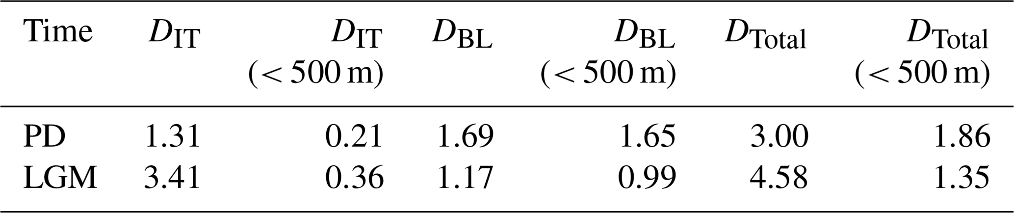
Figure 1 presents the bottom friction dissipation (DBL) and internal-tide dissipation (DIT) during the PD and the LGM. A significant difference in their distributions can be observed: bottom friction dissipation (DBL) is mainly concentrated in shallow sea areas, while internal-tide dissipation (DIT) is primarily found in deep-sea regions with notable topographic variations, such as mid-ocean ridges. Moreover, compared to the PD, primary regions of energy dissipation shifted from shallow to deep seas during the LGM. In the PD, dissipation below 500 m depth accounts for 1.86 TW, which is 62 % of the total dissipation. In contrast, during the LGM, dissipation below 500 m amounts to 1.35 TW, accounting for only 29 % of the total dissipation (Table 1). These data are consistent with previous research findings (Arbic et al., 2004a; Egbert et al., 2004; Green, 2010; Griffiths and Peltier, 2008, 2009; Wilmes and Green, 2014).
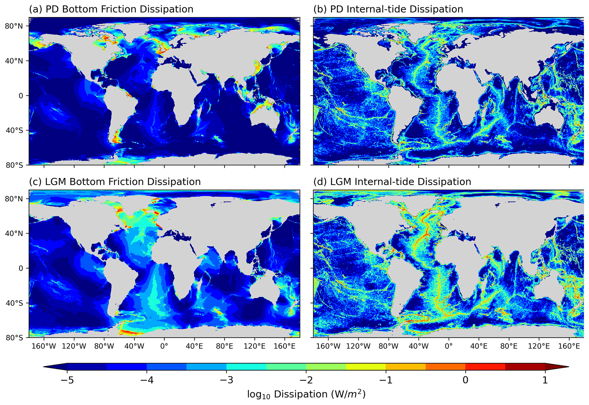
Figure 1Global distributions of bottom friction dissipation (DBL) and internal-tide dissipation (DIT) during the PD and LGM.
Table 1Global and sub-500 m distributions of DIT and DBL during the PD and LGM (measured in terawatts).
2.1.1 Bathymetry
The PD bathymetry data comes from the 1 min RTopo-2 database (Schaffer et al., 2016). For the LGM bathymetry, we use sea-level data from version 1.2 of ICE-5G (VM2 L90) (Peltier, 2004). Notably, tidal dissipation derived using ICE-6G is actually weaker than that obtained using ICE-5G (Wilmes et al., 2019; Wilmes et al., 2021). Here, we have chosen to use ICE-5G to investigate whether the AMOC during the LGM would have been affected by these stronger tidal conditions. The sea-level difference between the PD and LGM is calculated by subtracting the PD sea levels from the LGM sea levels obtained from the respective ICE-5G dataset. The low-resolution paleo-sea-level changes (1° horizontal resolution) are then interpolated to the RTopo-2 grid and added to the PD RTopo-2 bathymetry in order to retain the high-resolution topographic features. Finally, we interpolate the high-resolution bathymetry to the unstructured triangular mesh of the tidal model.
2.1.2 Tidal-model validation
The harmonically analyzed amplitudes (complex sinusoids) are used to evaluate the elevations. Simulated sinusoids () were interpolated to the 0.17° grid of TPXO9.v1 and compared to the reference sinusoids () by evaluating the spatially averaged root-mean-square (RMS) error (Δζ),
The RMS errors were calculated for four tidal constituents and determined separately for deep-water regions (depths > 500 m) and shallow shelf seas. The results are presented in Table 2. Meanwhile, Table 3 compares the M2 RMS error with the RMS errors of other forward tidal models.
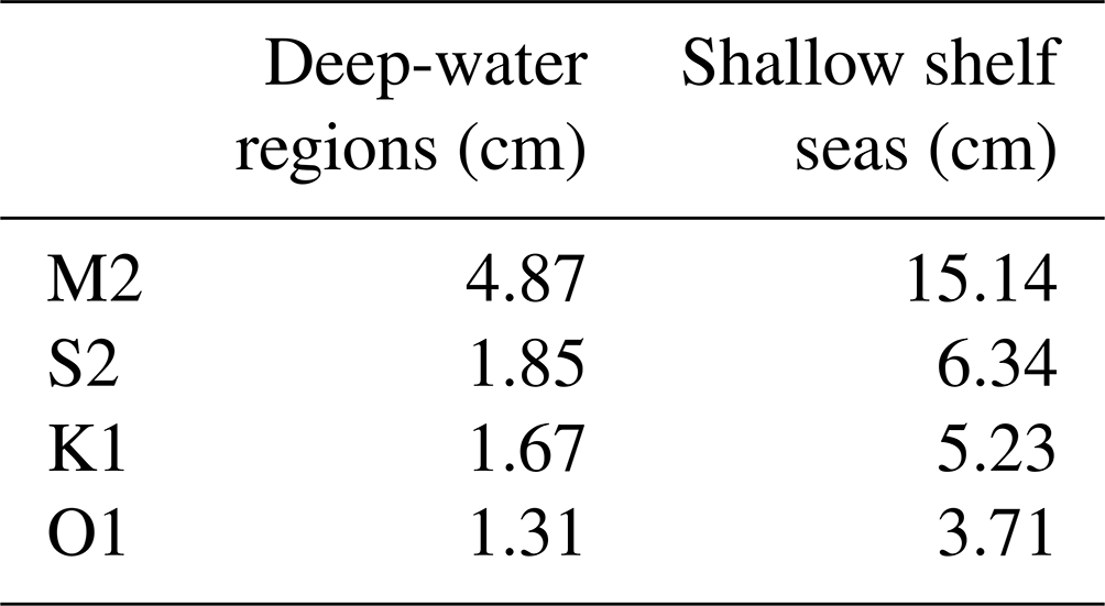
Table 3Comparison of M2 RMS errors in forward tidal models. Note that NA stands for not available.
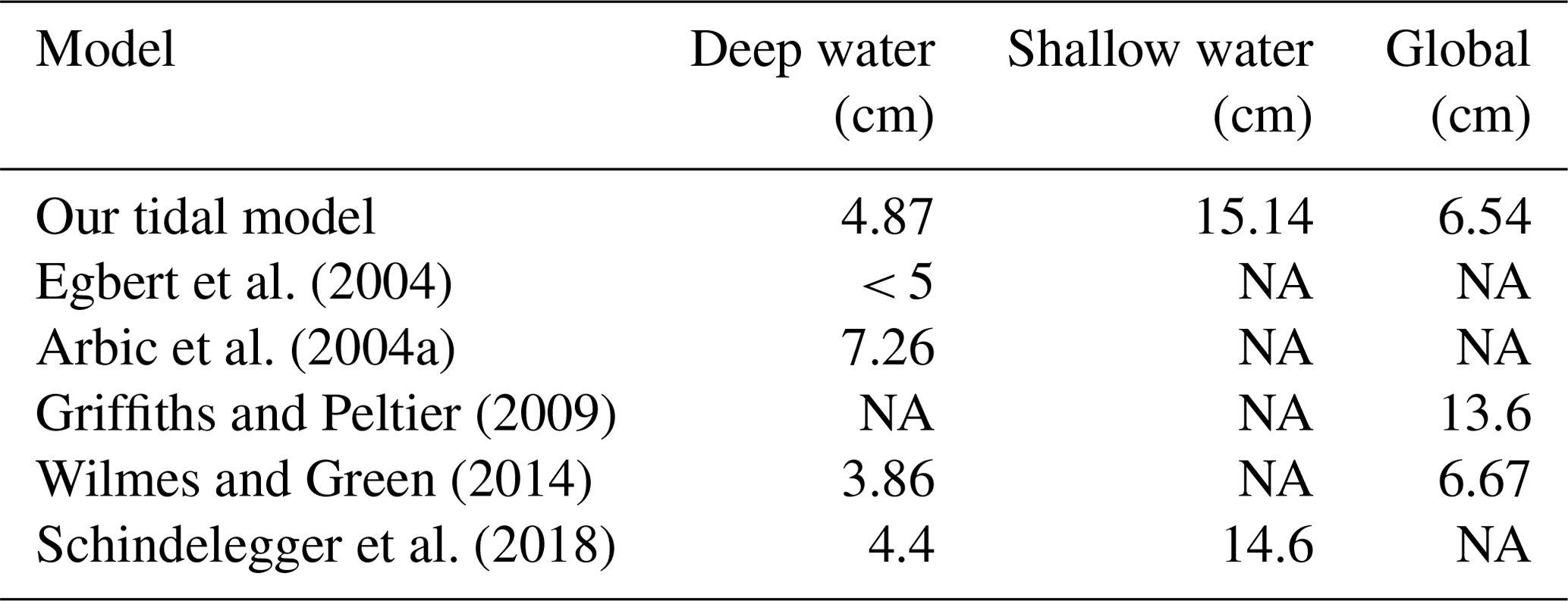
* Note that differences in the models selected across different studies may influence the results.
2.2 Ocean model
FESOM2.0 (Danilov et al., 2017), the ocean component of the Alfred Wegener Institute (AWI) Earth System Model (Sidorenko et al., 2019), is employed in our experiments. FESOM2.0 solves the primitive equations in the Boussinesq and hydrostatic approximations. It adopts an unstructured triangular-mesh framework, with scalar degrees of freedom located at vertices and horizontal velocities located at triangle centers. Additionally, the Finite-Element Sea Ice Model (FESIM; Danilov et al., 2015) is incorporated into FESOM2.0 as a set of subroutines. FESIM solves the modified elastic–viscous–plastic (mEVP) dynamical equations, enabling a reduction in subcycling steps while maintaining numerical stability (Kimmritz et al., 2017; Koldunov et al., 2019).
Figure 2 presents the horizontal resolution of the PD and LGM mesh configurations used in this study. The PD mesh consists of 126 858 nodes and 244 659 cells, while the LGM mesh comprises 104 425 nodes and 203 142 cells. Both meshes have the same nominal resolution of 1° for most parts of the global ocean, which translates to a resolution of approximately 25 km north of 50° N, a resolution of about 0.33° at the Equator, and a 10 km resolution for the Arctic Ocean and Bering Sea.
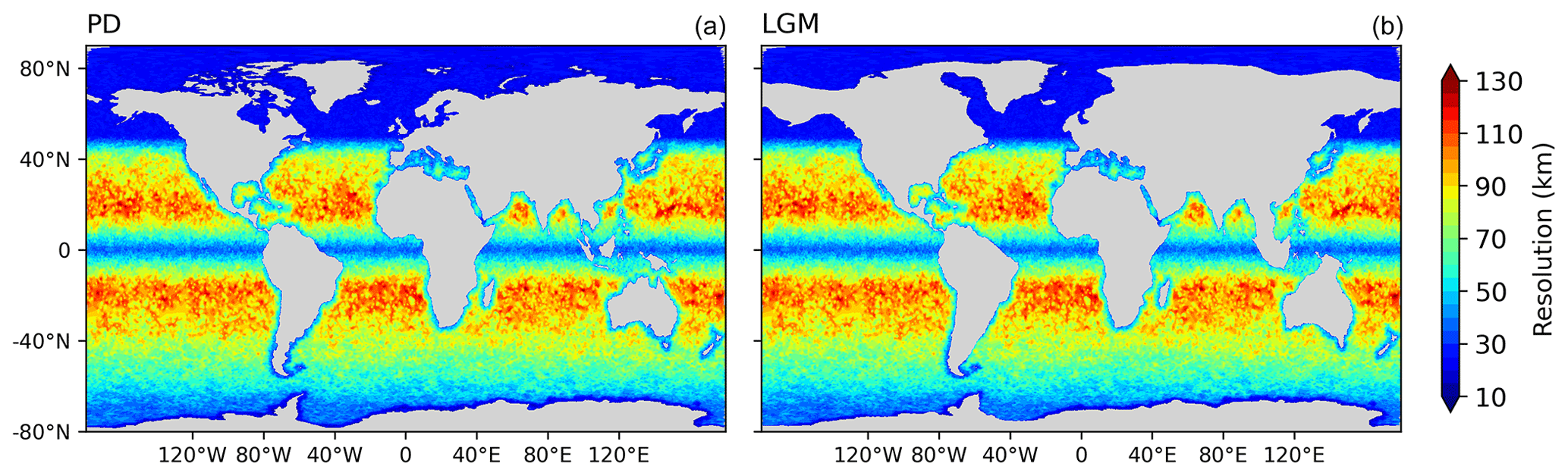
Figure 2Horizontal resolutions of the (a) PD and (b) LGM mesh configurations used in this study.
The K-profile parameterization (Large et al., 1994) is utilized universally for targeting surface ocean mixing, whereas a constant vertical background diffusivity (kbg) is employed to manage the effects of various background mixing mechanisms. In FESOM2.0, the default value for kbg is set to m2 s−1. Furthermore, the tidal-mixing parameterization by Schmittner and Egbert (2014), drawing on the foundational work of Jayne and St. Laurent (2001) and Simmons et al. (2004), is incorporated. This parameterization uniquely accounts for the influence of subgrid-scale bathymetry on the penetration depth of energy inputs and differentiates between diurnal and semidiurnal tidal effects. The tidal diapycnal diffusivity (kv_tidal) is given by
where Γ is the mixing efficiency, which is set to 0.2, and N2 is the buoyancy frequency. The rate of tidal-energy dissipation (ϵ) is given as
where is the internal-tide energy flux from barotropic tides to internal tides from the tidal model and F is the vertical decay function with an e-folding depth of 500 m above the seafloor (H). The local dissipation efficiency (qTC) accounts for the critical latitude (yc) of diurnal and semidiurnal tidal constituents (TCs):
where yc = 30° for the diurnal constituents (K1 and O1) and yc = 72° for the semidiurnal constituents (M2 and S2).
In the Methods section, we extract the internal-tide dissipation, denoted as DIT, from the global tidal model. In comparison to PD values, DIT for the four principal tidal constituents (M2, S2, K1, and O1) during the LGM shows almost a 3-fold increase, escalating from 1.31 to 3.41 TW (Table 1). The predominant contributor to this shift is the M2 tide, with a period of 12.42 h, which closely matches the North Atlantic basin's period of 12.66 h (Muller, 2008), creating resonance. During the LGM, the removal of continental shelves decreased damping, causing a significant increase in the M2 tide. Its value surged from a PD level of 0.89 TW and reached 2.94 TW during the LGM. These values are in close agreement with previous research findings (Arbic et al., 2004a; Egbert et al., 2004; Green, 2010; Griffiths and Peltier, 2008, 2009; Wilmes and Green, 2014). The horizontal distributions of DIT (Fig. 1) are used as input for a tidal-mixing parameterization in FESOM2.0.
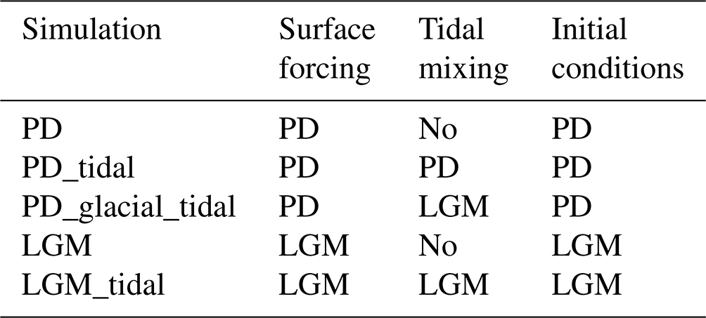
The experiments are designed to explore how tidal mixing impacts the glacial AMOC, with specifics outlined in Table 4. PD simulations are forced using the 1958–2020 period from the reanalysis dataset (JRA55-do v1.4.0) by Kobayashi et al. (2015), which represents the second global atmospheric reanalysis conducted by the Japan Meteorological Agency (JMA). As of 2009, it has employed the TL319 version of JMA's operational data assimilation system since 1958. The Japanese 55-year Reanalysis (JRA-55) addresses several issues identified in previous reanalyses and enhances the temporal consistency of temperature analysis, making it suitable for examining multidecadal variability and conducting climate simulations. We repeated each PD case simulation using the 1958–2020 JRA-55 data five times to achieve simulation stability. No significant trend was detected, and we utilized the average results from the final cycle for our analysis. The simulations conducted for the PD scenario using FESOM2.0 have been thoroughly validated. Detailed assessments and descriptions of the PD case's configuration can be found in Scholz et al. (2019) and (2022). Figure 3 presents a comparison of Atlantic Ocean temperature and salinity data from our PD case with World Ocean Atlas (WOA) 2018 data. The results indicate that our model accurately reproduces the temperature and salinity structures of the modern ocean. This provides a solid foundation for further simulations of the LGM ocean and the study of the role of tides.
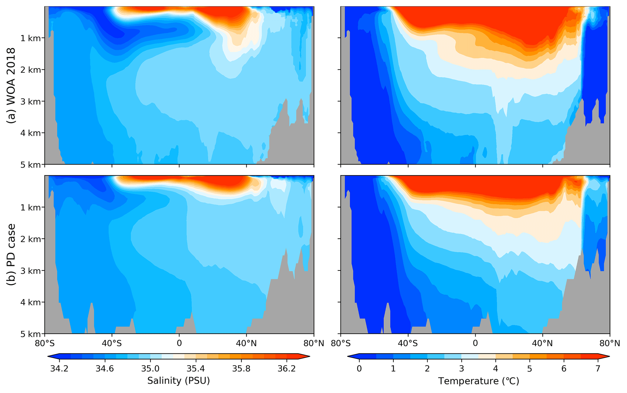
Figure 3Comparison of salinity and temperature between the WOA 2018 data and the PD simulation with respect to the Atlantic Ocean.
Regarding the LGM simulations, differences in model configuration are attributed to surface forcing and initial conditions. Both of these are taken from the LGMW case in Zhang et al. (2013). It is worth noting that selecting an appropriate forcing for the LGM simulations is crucial. In Knorr et al. (2021), a comparison of the LGM simulations of Atlantic Ocean temperature and salinity structure was conducted among different models from the Paleoclimate Modelling Intercomparison Project (PMIP; Braconnot et al., 2007; Weber et al., 2007) and the Coupled Model Intercomparison Project (CMIP; Braconnot et al., 2012; Kageyama et al., 2017). From these, we selected the simulation results from the well-performing climate model CoSMoS (Zhang et al., 2013) as the surface forcing for the LGM simulations in this study. This provides a solid foundation for accurately simulating the glacial ocean. The LGM simulations are executed over a duration of 600 years to achieve a quasi-equilibrium state. A time series depicting the strength of the AMOC in the LGM cases is presented in Fig. S1 in the Supplement. The concluding 62 years of this period were selected. The simulations are summarized in Table 4.
The AMOC strength varies between 11.6 and 15.5 Sv (sverdrups) for the PD and between 13.3 and 13.9 Sv for the LGM (Fig. 4; Table S1 in the Supplement). It is noteworthy that both LGM simulations (i.e., the LGM and LGM_tidal simulations) exhibit a shoaled AMOC, identified at approximately 1700 m depth. This suggests that the inclusion of tidal mixing does not affect the glacial AMOC's configuration. Instead, stratification is identified as a crucial factor contributing to the shoaled AMOC, which is more pronounced in the upper and middle regions of the glacial ocean. Stratification, on the one hand, signifies the buoyancy forces encountered by water masses during their descent. On the other hand, it exerts a notable influence on the model's tidal diffusivities, as outlined in Eq. (6). Our tidal-model results indicate that internal-tide dissipation (DIT) in the North Atlantic during the LGM reached 0.81 TW, a significant increase compared to the value of 0.13 TW observed in the PD, representing a 6-fold increase. Additionally, during the LGM, the average squared buoyancy frequency (N2) at depths of 1000–3000 m in the Atlantic corresponds to s−2, compared to s−2 in the PD. These changes do not suggest tidal dominance but rather imply a stronger vertical tidal diffusivity (shown in Fig. 4b and e). This enhanced vertical mixing aligns with the observed reductions in the vertical gradients of radiocarbon and δ13C in the deep Atlantic during the LGM (Skinner et al., 2017; Muglia et al., 2018; Peterson et al., 2014; Molina-Kescher et al., 2016; Sikes et al., 2016).
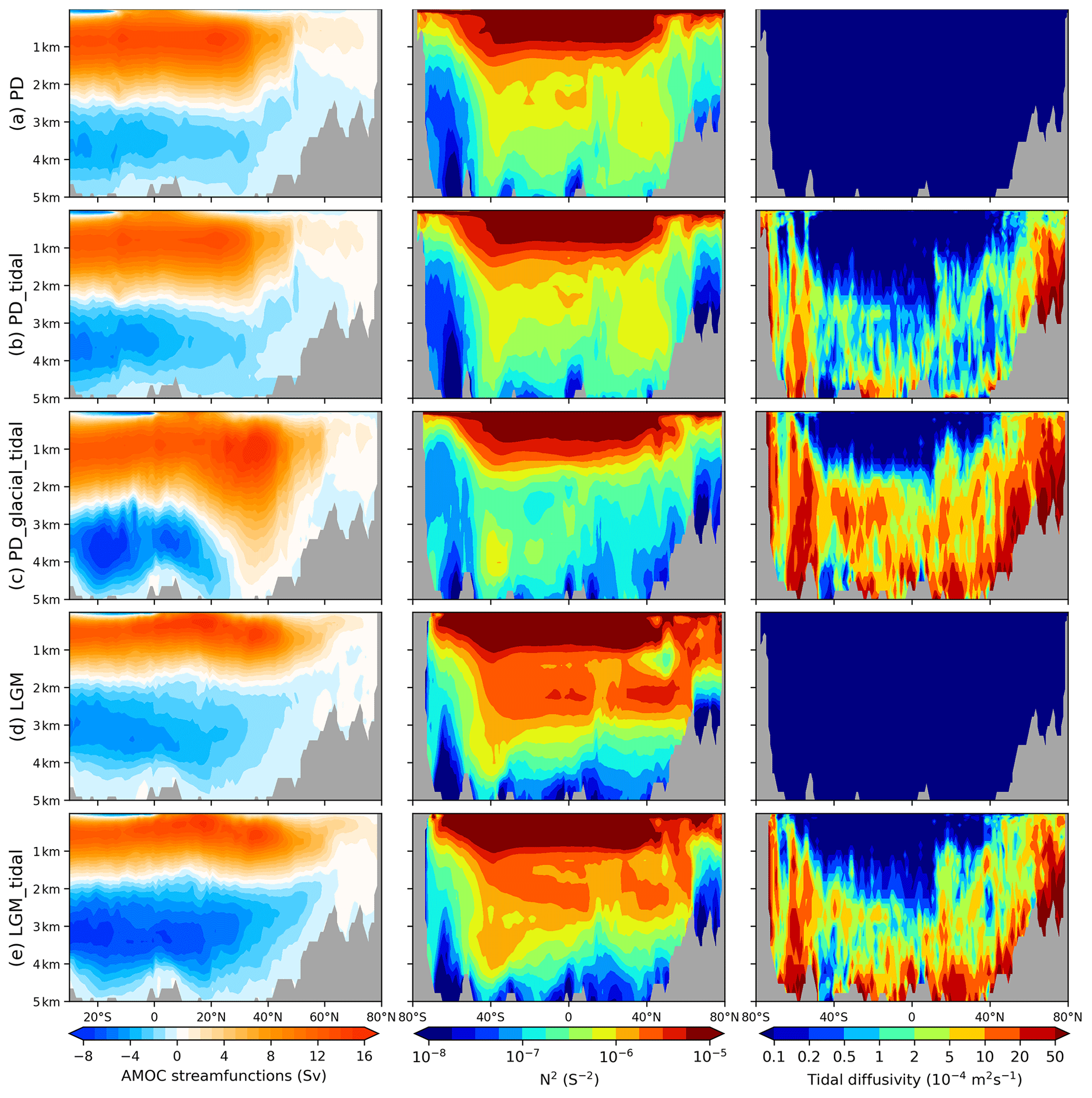
Figure 4Shown are the AMOC (left) as well as zonally averaged distributions for the squared buoyancy frequency (middle) and tidal diffusivity (right) across the Atlantic Ocean. Simulations are as listed in Table 4.
However, the incorporation of tidal-mixing processes results in a substantial increase in the generation of AABW, with a magnitude of −7.9 Sv, significantly exceeding the PD estimate of −4.2 Sv. This enhancement is in agreement with the results derived from paleoproxy data, which indicate intensified glacial AABW (Curry and Oppo, 2005; Zhang et al., 2017). Consequently, while LGM tides may not modify the AMOC, they exert a significant influence on AABW formation. Thus, accounting for tidal effects remains essential in conducting climate modeling for the LGM period.
In the PD_tidal experiment, incorporating the tidal-mixing parameterization does not alter the geometry of the AMOC. However, the PD_glacial_tidal simulation, which includes LGM tidal dissipation, reveals distinct dynamics. This simulation demonstrates a significant increase in both the strength and depth of the AMOC, extending to near-benthic layers at approximately 35° N (Fig. 4c and Table S1), and is accompanied by notably reduced stratification. These observations suggest that the effects and dynamics of enhanced tidal dissipation differ substantially under varying ocean stratification intensities during the LGM and PD periods.
To investigate the origins of various stratifications from the perspectives of temperature and salinity, we conduct a further analysis of the temperature and salinity distributions in the Atlantic Ocean across different cases (Fig. 5). Under PD forcing, the surface salinity below a latitude of 40° N is significantly higher than that in the middle and lower layers, which weakens ocean stratification. This sharply contrasts the high abyssal salinity observed during the LGM, a defining feature of the glacial ocean (Adkins et al., 2002; Knorr et al., 2021). Regarding temperature, a decrease from the surface to the seabed is observed in both the PD and LGM scenarios. Notably, during the LGM, the simulated temperature exhibits a pronounced decrease above a depth of 2 km, decreasing to 0 °C at this level. Below a depth of 2 km, the ocean is relatively homogeneous, with temperatures close to the freezing point, indicating a cold and well-mixed deep ocean, consistent with paleoproxy data (Adkins et al., 2002). This steeper temperature gradient enhances stratification in the upper layers of the glacial ocean. Collectively, the high abyssal salinity and swift vertical temperature decline significantly contribute to more pronounced stratification within the glacial ocean. Accurately replicating these temperature and salinity features is crucial in the climate modeling of the LGM.
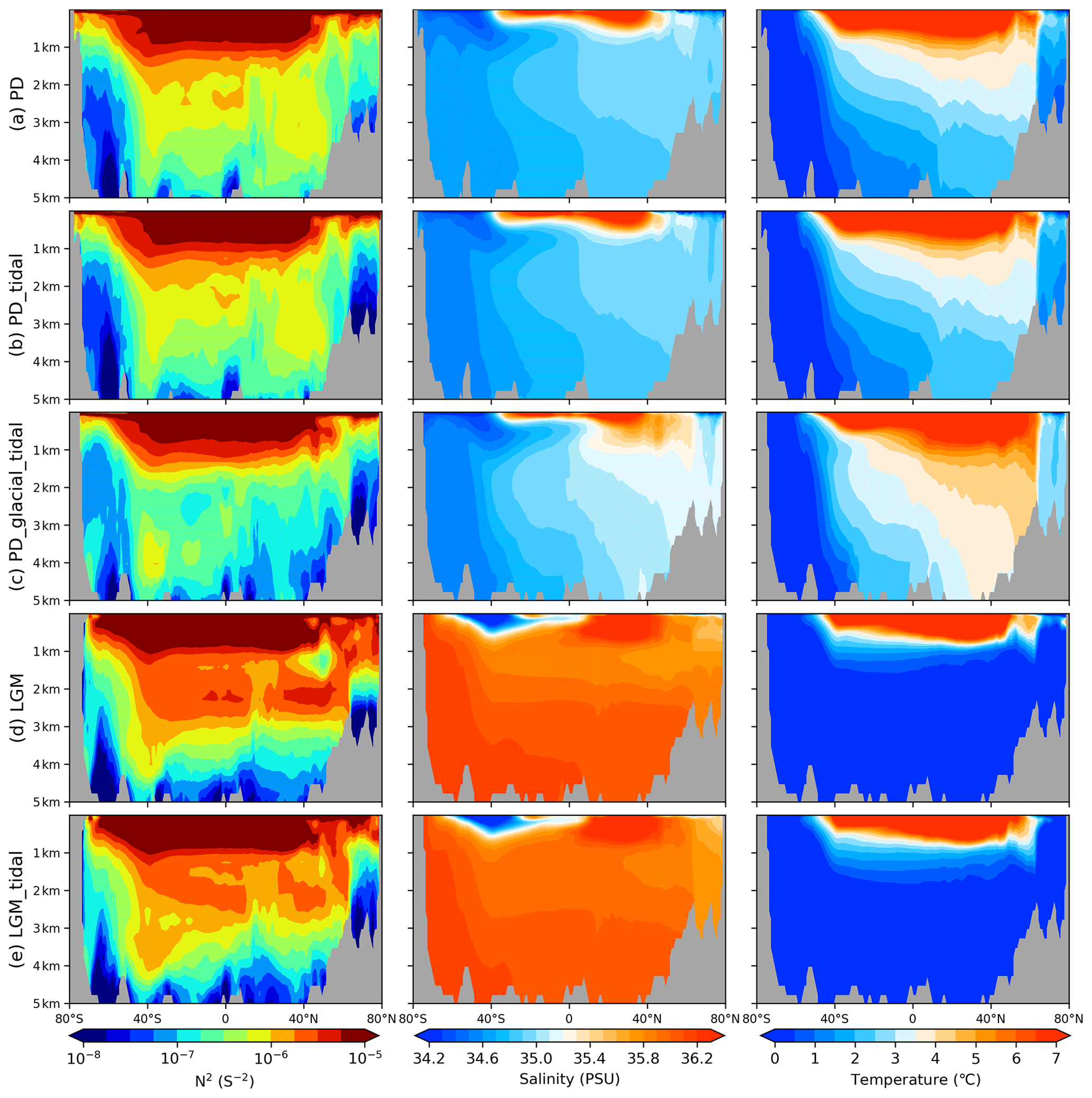
Figure 5Zonally averaged distributions across the Atlantic Ocean for the simulations listed in Table 4. The distributions for the squared buoyancy frequency (left), salinity (middle), and potential temperature (right) are shown.
In our comparable consideration of enhanced tidal mixing during the LGM, the discrepancy between our results and those of previous studies (Schmittner et al., 2015; Wilmes et al., 2019) is attributed to the fact that these studies do not reproduce high abyssal salinity and increased stratification in the LGM Atlantic. These features counteract the impact of stronger tidal mixing on the AMOC.
Tides play a pivotal role in climate dynamics, e.g., by facilitating the release of iceberg armadas during Heinrich events (Arbic et al., 2004b) and serving as the primary driving force behind both vertical and horizontal ice sheet movements at the corresponding marine peripheries (Padman et al., 2018). Focusing on the LGM period reveals that glacial tidal dissipation was approximately 3 times greater than present levels. This increase, combined with the closure of the Bering Strait (Hu et al., 2010), led to reduced freshwater transport to the Atlantic, ostensibly resulting in a strengthened glacial AMOC. However, paleoclimatic proxy data indicate a significant shoaling of the AMOC during the LGM, with an estimated reduction in depth of about 1000 m compared to contemporary conditions (Burke et al., 2015; Lund et al., 2011). The primary aim of this study is to identify the reasons for the shoaled glacial AMOC given the complex interplay of these factors.
Our results indicate that the integration of additional tidal-mixing parameterizations does not significantly influence the AMOC in either the PD or the LGM scenarios. In the PD scenario, the relatively weak tides can be adequately accounted for by background diffusivity (kbg), thereby negating the necessity for an additional tidal parameterization. Furthermore, during the LGM, tides are unlikely to have played a substantial role in influencing the glacial AMOC due to pronounced ocean stratification. On the one hand, this stratification hampers the mixing of water masses, while on the other hand, it leads to a decrease in the effectiveness of tidal mixing. This is because the buoyancy frequency, which appears in the denominator of the tidal-mixing parameterization (as detailed in Eq. 6 in the Method section), suggests that stronger stratification significantly reduces the impact of tidal dissipation. However, in the abyssal ocean, where there is relatively weak stratification, the pronounced tidal dissipation during the LGM notably enhances the formation of AABW.
The tidal-mixing parameterization only considers locally dissipated energy, which only accounts for one-third of the total energy (Jayne, 2009; Schmittner and Egbert, 2014). The remaining two-thirds of the energy is dissipated in the far-field, where background diffusivity (kbg) is employed to represent this dissipation. Consequently, we calculated the far-field dissipation due to kbg and the local tidal dissipation due to kv_tidal for each simulation using the Osborn (1980) formula, expressed as follows:
The results are presented in Table 5. Additionally, we conducted another experiment, LGM_tidal_3, in which kbg increased from to m2 s−1 for comparison. The results indicate that the LGM_tidal experiment underestimates tidal energy, reaching only 2.05 TW. In contrast, the LGM_tidal_3 experiment shows no such underestimation, with its energy reaching 3.92 TW.
Table 5Summary of the energy consumption due to diapycnal mixing.
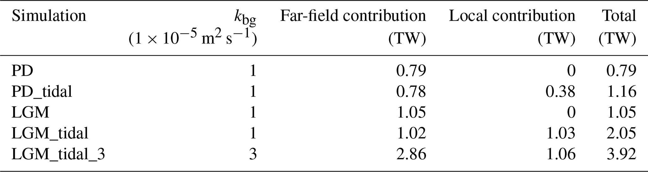
Figure 6 presents the AMOC geometry for the LGM_tidal and LGM_tidal_3 experiments. The geometry of the AMOC in LGM_tidal_3 experiment remains relatively shallow, without significant changes, which further supports our study's conclusions. The only notable change is in the AMOC strength, which increased from 13.3 to 15.4 Sv. This underscores the necessity of employing the tidal-mixing parameterization and the importance of appropriately adjusting the background diffusivity (kbg). Additionally, this result is the first to demonstrate that the shallower geometry of the glacial AMOC during the LGM remains unchanged, even when accounting for far-field tidal dissipation.
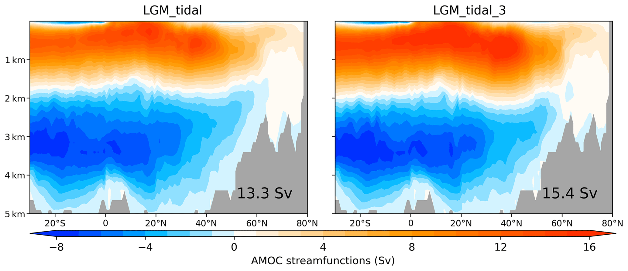
Figure 6AMOC stream functions (measured in sverdrups) for the LGM_tidal and LGM_tidal_3 simulations.
Applying enhanced LGM tidal dissipation to PD conditions (in the case of the PD_glacial_tidal simulation), where ocean stratification is significantly weaker than that under LGM conditions, yields entirely different results. In this scenario, the amplified tidal dissipation induces a deeper and more potent AMOC. We propose a potential positive feedback mechanism that accounts for the increased AMOC during termination. A reduced ocean stratification during the initial phase of termination enhances the effectiveness of tidal mixing, a process analogous to the one discussed above. This increased tidal mixing will affect the ocean more efficiently, further weakening ocean stratification, thereby increasing tidal mixing. This initiates a positive feedback loop that culminates in reduced stratification and a more vigorous and deeper AMOC.
The concept of enhanced glacial-ocean stratification, which potentially results from the cooling and salinification of glacial AABW and could lead to a shoaled AMOC during the LGM, has previously been discussed (Jansen and Nadeau, 2016; Jansen, 2017; Klockmann et al., 2016). However, until now, no research has directly demonstrated a shoaled AMOC under real LGM forcing conditions, including the impact of increased glacial tidal dissipation. Montenegro et al. (2007) proposed that LGM tides have a minimal impact on the AMOC, attributing this to a potential underestimation of tidal dissipation during the LGM. In contrast, Schmittner et al. (2015) and Wilmes et al. (2019) suggested a significant enhancement and deepening of the North Atlantic overturning cell under vigorous glacial tidal dissipation. It is noteworthy that Wilmes et al. (2021) obtained a relatively shoaled LGM AMOC through the artificial reduction of meridional moisture flux and precipitation at high latitudes.
Our study is the first to directly demonstrate a stratified ocean and a shoaled AMOC under real LGM forcing conditions, without any artificial modifications, despite the presence of increased glacial tidal dissipation. We suggest that accurately simulating the high salinity of the deep sea and the rapid temperature changes in the ocean's upper layers is crucial for correctly reproducing a stratified glacial ocean. In such an environment, the significant tidal dissipation during the LGM was not sufficient enough to counter the increased ocean stratification, leading to a shoaled AMOC. Furthermore, we emphasize that this notable glacial tidal dissipation plays a critical role in strengthening AABW during the LGM.
Our results highlight the dominance of background conditions and mixing with respect to ocean circulation dynamics, as well as possible complex feedbacks in the Earth system (Lohmann et al., 2020). Here, we use an ocean-only model, which means the LGM atmospheric forcing is kept constant. Consequently, this approach has a limitation: it does not account for interactions between the ocean (or sea ice) and the atmosphere. As a logical next step, we plan to incorporate tidal-energy dissipation into fully coupled Earth system models (Zhang et al., 2014; Liu et al., 2009) to further explore AMOC dynamics during deglaciation.
To address the N2 sensitivities and interactions between FESOM2.0 and the tidal model, we employed an iterative process for the PD_tidal and LGM_tidal simulations. Here, we provide a detailed description of this process, employing the LGM_tidal simulation as an example.
The steps of the iterative process are as follows:
-
For the initial input, we begin by obtaining N2 from the LGM simulation, which does not include tidal mixing. This initial N2 is then used as input for the tidal model.
-
In the first iteration (LGM_tidal1), the tidal model, which uses the initial N2, calculates the tidal dissipation, which is then fed back into FESOM2.0, producing the first experimental result (LGM_tidal1).
-
In the second iteration (LGM_tidal2), N2 from the LGM_tidal1 simulation is inputted into the tidal model once again to generate a new tidal dissipation, which is incorporated into FESOM2.0, and the model is run to obtain LGM_tidal2.
-
The final output (LGM_tidal2) represents the second iteration and is the LGM_tidal experiment presented in our paper.
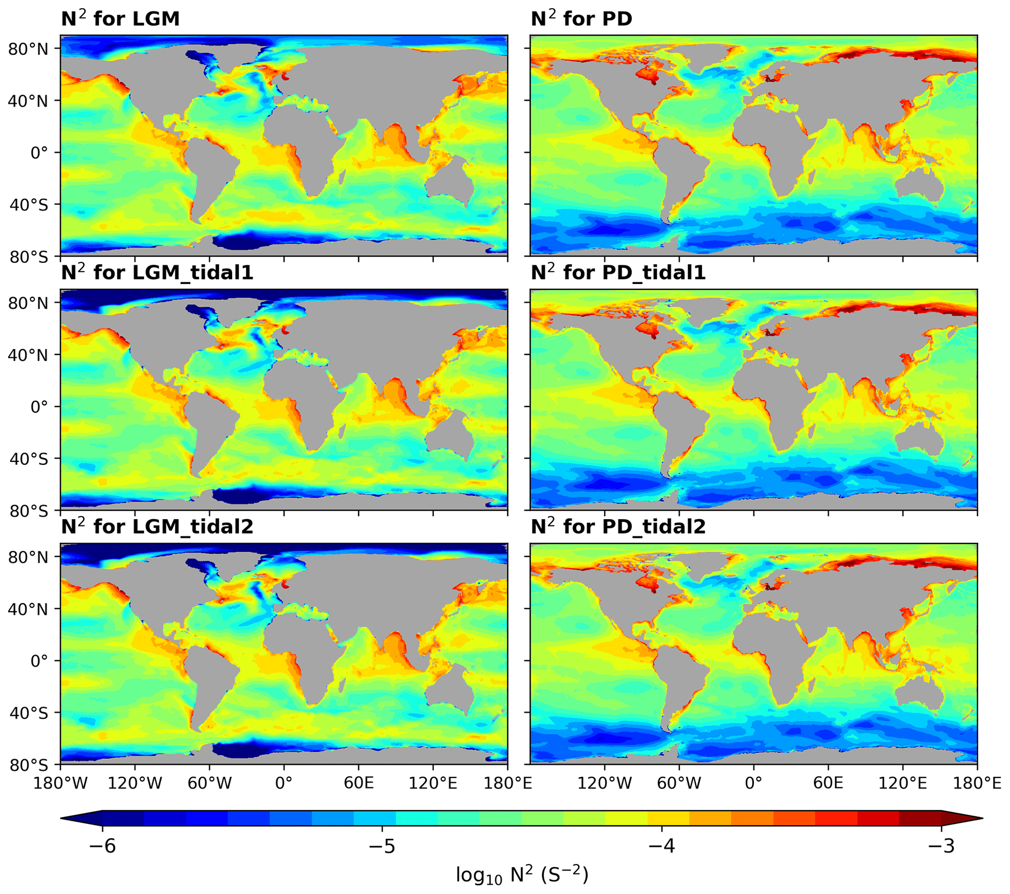
Figure A1Changes in depth-averaged vertical N2 values across iterations for the LGM and PD simulations.
Fig. A1 illustrates the changes in depth-averaged vertical N2 values during these iterations for both the PD and LGM scenarios. For the LGM simulations, the primary change from the initial LGM iteration to the LGM_tidal1 iteration involved a decrease in N2 in the Arctic, and from the LGM_tidal1 iteration to the LGM_tidal2 iteration, minimal changes were observed. However, for the PD simulations, no significant changes in N2 were observed throughout the iterations, effectively minimizing the mutual influences between N2 in the tidal model and that in the OGCM after the iterative process. This iterative approach ensures the stability and accuracy of our model results, reducing the sensitivity of N2 to tidal-dissipation feedbacks.
The FESOM2 model is described by Danilov et al. (2017), and the code used in this study can be accessed at https://github.com/FESOM/fesom2 (Scholz, 2024). The simulations require additional atmospheric-forcing files. The Last Glacial Maximum (LGM) atmospheric-forcing data are from Zhang et al. (2013). The data for present-day (PD) forcing used in this study are from Kobayashi et al. (2015), including the JRA-55 dataset (http://jra.kishou.go.jp/JRA-55/index_en.html, JMA, 2024). The final 62-year-averaged results of the simulations used in this study are available on Zenodo (https://doi.org/10.5281/zenodo.13709813, Chen, 2024). If the full output data are required, they can be requested by contacting the corresponding author.
The supplement related to this article is available online at: https://doi.org/10.5194/cp-20-2001-2024-supplement.
YC and GL conceived and designed the study. YC developed and performed the model simulations under the guidance of PS, GL, and XC. All authors contributed to writing and revising the paper.
The contact author has declared that none of the authors has any competing interests.
Publisher’s note: Copernicus Publications remains neutral with regard to jurisdictional claims made in the text, published maps, institutional affiliations, or any other geographical representation in this paper. While Copernicus Publications makes every effort to include appropriate place names, the final responsibility lies with the authors.
We appreciate the discussions with Dehai Song and Hu Yang that have been had during the course of this work. Furthermore, we extend our sincere thanks to the HPC department of the Alfred Wegener Institute (AWI) and the German Climate Computation Center (DKRZ) for their support. Special thanks are due to the handling editor, Marisa Montoya, for her meticulous work and to Guido Vettoretti and an anonymous reviewer for their constructive comments and suggestions.
Xianyao Chen is supported by the National Natural Science Foundation of China under grant no. 42394130 and by the National Key R&D Program of China under grant no. 2019YFA0607000. Gerrit Lohmann receives funding through the “Ocean and Cryosphere under climate change” project within the “Changing Earth – Sustaining our Future” program offered by the Helmholtz Society and through the Bundesministerium für Bildung und Forschung (grant nos. 01LP1917A and 01LP2004A).
The article processing charges for this open-access publication were covered by the Alfred-Wegener-Institut, Helmholtz-Zentrum für Polar- und Meeresforschung.
This paper was edited by Marisa Montoya and reviewed by Guido Vettoretti and one anonymous referee.
Adkins, J. F., McIntyre, K., and Schrag, D. P.: The salinity, temperature, and δ18O of the glacial deep ocean, Science, 298, 1769–1773, https://doi.org/10.1126/science.1076252, 2002.
Arbic, B. K., Garner, S. T., Hallberg, R. W., and Simmons, H. L.: The accuracy of surface elevations in forward global barotropic and baroclinic tide models, Deep-Sea Res. Pt. II, 51, 3069–3101, https://doi.org/10.1016/j.dsr2.2004.09.014, 2004a.
Arbic, B. K., Macayeal, D. R., Mitrovica, J. X., and Milne, G. A.: Palaeoclimate – Ocean tides and Heinrich events, Nature, 432, 460–460, 10.1038/432460a, 2004b.
Baker, J. A., Watson, A. J., and Vallis, G. K.: Meridional Overturning Circulation in a Multibasin Model. Part I: Dependence on Southern Ocean Buoyancy Forcing, J. Phys. Oceanogr., 50, 1159–1178, https://doi.org/10.1175/Jpo-D-19-0135.1, 2020.
Bouttes, N., Roche, D. M., and Paillard, D.: Impact of strong deep ocean stratification on the glacial carbon cycle, Paleoceanography, 24, Pa3203, https://doi.org/10.1029/2008pa001707, 2009.
Boyle, E. A. and Keigwin, L.: North-Atlantic Thermohaline Circulation during the Past 20,000 Years Linked to High-Latitude Surface-Temperature, Nature, 330, 35–40, https://doi.org/10.1038/330035a0, 1987.
Braconnot, P., Otto-Bliesner, B., Harrison, S., Joussaume, S., Peterchmitt, J.-Y., Abe-Ouchi, A., Crucifix, M., Driesschaert, E., Fichefet, Th., Hewitt, C. D., Kageyama, M., Kitoh, A., Loutre, M.-F., Marti, O., Merkel, U., Ramstein, G., Valdes, P., Weber, L., Yu, Y., and Zhao, Y.: Results of PMIP2 coupled simulations of the Mid-Holocene and Last Glacial Maximum – Part 2: feedbacks with emphasis on the location of the ITCZ and mid- and high latitudes heat budget, Clim. Past, 3, 279–296, https://doi.org/10.5194/cp-3-279-2007, 2007.
Braconnot, P., Harrison, S. P., Kageyama, M., Bartlein, P. J., Masson-Delmotte, V., Abe-Ouchi, A., Otto-Bliesner, B., and Zhao, Y.: Evaluation of climate models using palaeoclimatic data, Nat. Clim. Change, 2, 417–424, 10.1038/Nclimate1456, 2012.
Broecker, W. S. and Hemming, S.: Paleoclimate – Climate swings come into focus, Science, 294, 2308–2309, https://doi.org/10.1126/science.1068389, 2001.
Burke, A., Stewart, A. L., Adkins, J. F., Ferrari, R., Jansen, M. F., and Thompson, A. F.: The glacial mid-depth radiocarbon bulge and its implications for the overturning circulation, Paleoceanography, 30, 1021–1039, 10.1002/2015pa002778, 2015.
Butzin, M., Prange, M., and Lohmann, G.: Radiocarbon simulations for the glacial ocean: The effects of wind stress, Southern Ocean sea ice and Heinrich events, Earth Planet. Sc. Lett., 235, 45–61, 10.1016/j.epsl.2005.03.003, 2005.
Chen, C. S., Liu, H. D., and Beardsley, R. C.: An unstructured grid, finite-volume, three-dimensional, primitive equations ocean model: Application to coastal ocean and estuaries, J. Atmos. Ocean. Tech., 20, 159–186, https://doi.org/10.1175/1520-0426(2003)020<0159:Augfvt>2.0.Co;2, 2003.
Chen, Y.: Chen et al. (2024) supplement (Climate of the past): The output for the Last Glacial Maximum (LGM) and the Present Day (PD) simulations, Zenodo [data set], https://doi.org/10.5281/zenodo.13709813, 2024.
Clark, P. U., Pisias, N. G., Stocker, T. F., and Weaver, A. J.: The role of the thermohaline circulation in abrupt climate change, Nature, 415, 863–869, https://doi.org/10.1038/415863a, 2002.
Curry, W. B. and Oppo, D. W.: Glacial water mass geometry and the distribution of δ13C of Sigma CO2 in the western Atlantic Ocean, Paleoceanography, 20, Pa1017, https://doi.org/10.1029/2004pa001021, 2005.
Danilov, S., Wang, Q., Timmermann, R., Iakovlev, N., Sidorenko, D., Kimmritz, M., Jung, T., and Schröter, J.: Finite-Element Sea Ice Model (FESIM), version 2, Geosci. Model Dev., 8, 1747–1761, https://doi.org/10.5194/gmd-8-1747-2015, 2015.
Danilov, S., Sidorenko, D., Wang, Q., and Jung, T.: The Finite-volumE Sea ice–Ocean Model (FESOM2), Geosci. Model Dev., 10, 765–789, https://doi.org/10.5194/gmd-10-765-2017, 2017.
Duplessy, J. C., Shackleton, N. J., Fairbanks, R. G., Labeyrie, L., Oppo, D., and Kallel, N.: Deepwater source variations during the last climatic cycle and their impact on the global deepwater circulation, Paleoceanography, 3, 343–360, https://doi.org/10.1029/PA003i003p00343, 1988.
Egbert, G. D. and Ray, R. D.: Semi-diurnal and diurnal tidal dissipation from TOPEX/Poseidon altimetry, Geophys. Res. Lett., 30, 1907, https://doi.org/10.1029/2003gl017676, 2003.
Egbert, G. D., Ray, R. D., and Bills, B. G.: Numerical modeling of the global semidiurnal tide in the present day and in the last glacial maximum, J. Geophys. Res.-Oceans, 109, C03003, https://doi.org/10.1029/2003jc001973, 2004.
Ferrari, R. and Wunsch, C.: Ocean Circulation Kinetic Energy: Reservoirs, Sources, and Sinks, Annu. Rev. Fluid Mech., 41, 253–282, https://doi.org/10.1146/annurev.fluid.40.111406.102139, 2009.
Ferrari, R., Jansen, M. F., Adkins, J. F., Burke, A., Stewart, A. L., and Thompson, A. F.: Antarctic sea ice control on ocean circulation in present and glacial climates, P. Natl. Acad. Sci. USA, 111, 8753–8758, 10.1073/pnas.1323922111, 2014.
Francois, R., Altabet, M. A., Yu, E. F., Sigman, D. M., Bacon, M. P., Frank, M., Bohrmann, G., Bareille, G., and Labeyrie, L. D.: Contribution of Southern Ocean surface-water stratification to low atmospheric CO2 concentrations during the last glacial period, Nature, 389, 929–935, https://doi.org/10.1038/40073, 1997.
Ganopolski, A. and Rahmstorf, S.: Rapid changes of glacial climate simulated in a coupled climate model, Nature, 409, 153–158, https://doi.org/10.1038/35051500, 2001.
Gordon, A. L.: Interocean exchange of thermocline water, J. Geophys. Res., 91, 5037–5046, https://doi.org/10.1029/JC091iC04p05037, 1986.
Green, J. A. M.: Ocean tides and resonance, Ocean Dynam., 60, 1243–1253, https://doi.org/10.1007/s10236-010-0331-1, 2010.
Green, J. A. M., Green, C. L., Bigg, G. R., Rippeth, T. P., Scourse, J. D., and Uehara, K.: Tidal mixing and the Meridional Overturning Circulation from the Last Glacial Maximum, Geophys. Res. Lett., 36, L15603, https://doi.org/10.1029/2009gl039309, 2009.
Griffiths, S. D. and Peltier, W. R.: Megatides in the Arctic Ocean under glacial conditions, Geophys. Res. Lett., 35, L08605, https://doi.org/10.1029/2008gl033263, 2008.
Griffiths, S. D. and Peltier, W. R.: Modeling of Polar Ocean Tides at the Last Glacial Maximum: Amplification, Sensitivity, and Climatological Implications, J. Climate, 22, 2905–2924, https://doi.org/10.1175/2008jcli2540.1, 2009.
Hendershott, M. C.: Effects of Solid Earth Deformation on Global Ocean Tides, Geophys. J. Roy Astr. S, 29, 389–402, https://doi.org/10.1111/j.1365-246X.1972.tb06167.x, 1972.
Hesse, T., Butzin, M., Bickert, T., and Lohmann, G.: A model-data comparison ofδ13C in the glacial Atlantic Ocean, Paleoceanography, 26, PA3220, https://doi.org/10.1029/2010pa002085, 2011.
Hu, A. X., Meehl, G. A., Otto-Bliesner, B. L., Waelbroeck, C., Han, W. Q., Loutre, M. F., Lambeck, K., Mitrovica, J. X., and Rosenbloom, N.: Influence of Bering Strait flow and North Atlantic circulation on glacial sea-level changes, Nat. Geosci., 3, 118–121, https://doi.org/10.1038/Ngeo729, 2010.
Jansen, M. F.: Glacial ocean circulation and stratification explained by reduced atmospheric temperature, P. Natl. Acad. Sci. USA, 114, 45–50, https://doi.org/10.1073/pnas.1610438113, 2017.
Jansen, M. F. and Nadeau, L. P.: The Effect of Southern Ocean Surface Buoyancy Loss on the Deep-Ocean Circulation and Stratification, J. Phys. Oceanogr., 46, 3455–3470, https://doi.org/10.1175/Jpo-D-16-0084.1, 2016.
Jayne, S. R.: The Impact of Abyssal Mixing Parameterizations in an Ocean General Circulation Model, J. Phys. Oceanogr., 39, 1756–1775, https://doi.org/10.1175/2009jpo4085.1, 2009.
Jayne, S. R. and St. Laurent, L. C.: Parameterizing tidal dissipation over rough topography, Geophys. Res. Lett., 28, 811–814, https://doi.org/10.1029/2000gl012044, 2001.
JMA – Japan Meteorological Agency: Japanese 55-year Reanalysis, JMA [data set], http://jra.kishou.go.jp/JRA-55/index_en.html, last access: 25 March 2024.
Kageyama, M., Albani, S., Braconnot, P., Harrison, S. P., Hopcroft, P. O., Ivanovic, R. F., Lambert, F., Marti, O., Peltier, W. R., Peterschmitt, J.-Y., Roche, D. M., Tarasov, L., Zhang, X., Brady, E. C., Haywood, A. M., LeGrande, A. N., Lunt, D. J., Mahowald, N. M., Mikolajewicz, U., Nisancioglu, K. H., Otto-Bliesner, B. L., Renssen, H., Tomas, R. A., Zhang, Q., Abe-Ouchi, A., Bartlein, P. J., Cao, J., Li, Q., Lohmann, G., Ohgaito, R., Shi, X., Volodin, E., Yoshida, K., Zhang, X., and Zheng, W.: The PMIP4 contribution to CMIP6 – Part 4: Scientific objectives and experimental design of the PMIP4-CMIP6 Last Glacial Maximum experiments and PMIP4 sensitivity experiments, Geosci. Model Dev., 10, 4035–4055, https://doi.org/10.5194/gmd-10-4035-2017, 2017.
Kageyama, M., Harrison, S. P., Kapsch, M.-L., Lofverstrom, M., Lora, J. M., Mikolajewicz, U., Sherriff-Tadano, S., Vadsaria, T., Abe-Ouchi, A., Bouttes, N., Chandan, D., Gregoire, L. J., Ivanovic, R. F., Izumi, K., LeGrande, A. N., Lhardy, F., Lohmann, G., Morozova, P. A., Ohgaito, R., Paul, A., Peltier, W. R., Poulsen, C. J., Quiquet, A., Roche, D. M., Shi, X., Tierney, J. E., Valdes, P. J., Volodin, E., and Zhu, J.: The PMIP4 Last Glacial Maximum experiments: preliminary results and comparison with the PMIP3 simulations, Clim. Past, 17, 1065–1089, https://doi.org/10.5194/cp-17-1065-2021, 2021.
Kimmritz, M., Losch, M., and Danilov, S.: A comparison of viscous-plastic sea ice solvers with and without replacement pressure, Ocean Model., 115, 59–69, https://doi.org/10.1016/j.ocemod.2017.05.006, 2017.
Klockmann, M., Mikolajewicz, U., and Marotzke, J.: The effect of greenhouse gas concentrations and ice sheets on the glacial AMOC in a coupled climate model, Clim. Past, 12, 1829–1846, https://doi.org/10.5194/cp-12-1829-2016, 2016.
Knorr, G. and Lohmann, G.: Southern Ocean origin for the resumption of Atlantic thermohaline circulation during deglaciation, Nature, 424, 532–536, https://doi.org/10.1038/nature01855, 2003.
Knorr, G., Barker, S., Zhang, X., Lohmann, G., Gong, X., Gierz, P., Stepanek, C., and Stap, L. B.: A salty deep ocean as a prerequisite for glacial termination, Nat. Geosci., 14, 930–936, https://doi.org/10.1038/s41561-021-00857-3, 2021.
Kobayashi, S., Ota, Y., Harada, Y., Ebita, A., Moriya, M., Onoda, H., Onogi, K., Kamahori, H., Kobayashi, C., Endo, H., Miyaoka, K., and Takahashi, K.: The JRA-55 Reanalysis: General Specifications and Basic Characteristics, J. Meteorol. Soc. Jpn., 93, 5–48, https://doi.org/10.2151/jmsj.2015-001, 2015.
Koldunov, N. V., Aizinger, V., Rakowsky, N., Scholz, P., Sidorenko, D., Danilov, S., and Jung, T.: Scalability and some optimization of the Finite-volumE Sea ice–Ocean Model, Version 2.0 (FESOM2), Geosci. Model Dev., 12, 3991–4012, https://doi.org/10.5194/gmd-12-3991-2019, 2019.
Large, W. G., Mcwilliams, J. C., and Doney, S. C.: Oceanic Vertical Mixing – a Review and a Model with a Nonlocal Boundary-Layer Parameterization, Rev. Geophys., 32, 363–403, https://doi.org/10.1029/94rg01872, 1994.
Ledbetter, M. T. and Johnson, D. A.: Increased Transport of Antarctic Bottom Water in the Vema Channel During the Last Ice Age, Science, 194, 837–839, https://doi.org/10.1126/science.194.4267.837, 1976.
Lippold, J., Luo, Y. M., Francois, R., Allen, S. E., Gherardi, J., Pichat, S., Hickey, B., and Schulz, H.: Strength and geometry of the glacial Atlantic Meridional Overturning Circulation, Nat. Geosci., 5, 813–816, https://doi.org/10.1038/Ngeo1608, 2012.
Liu, Z., Otto-Bliesner, B. L., He, F., Brady, E. C., Tomas, R., Clark, P. U., Carlson, A. E., Lynch-Stieglitz, J., Curry, W., Brook, E., Erickson, D., Jacob, R., Kutzbach, J., and Cheng, J.: Transient Simulation of Last Deglaciation with a New Mechanism for Bolling-Allerod Warming, Science, 325, 310–314, https://doi.org/10.1126/science.1171041, 2009.
Lohmann, G., Butzin, M., Eissner, N., Shi, X. X., and Stepanek, C.: Abrupt Climate and Weather Changes Across Time Scales, Paleoceanography and Paleoclimatology, 35, e2019PA003782, https://doi.org/10.1029/2019PA003782, 2020.
Lund, D. C., Adkins, J. F., and Ferrari, R.: Abyssal Atlantic circulation during the Last Glacial Maximum: Constraining the ratio between transport and vertical mixing, Paleoceanography, 26, PA1213, https://doi.org/10.1029/2010pa001938, 2011.
Lynch-Stieglitz, J., Adkins, J. F., Curry, W. B., Dokken, T., Hall, I. R., Herguera, J. C., Hirschi, J. J. M., Ivanova, E. V., Kissel, C., Marchal, O., Marchitto, T. M., McCave, I. N., McManus, J. F., Mulitza, S., Ninnemann, U., Peeters, F., Yu, E. F., and Zahn, R.: Atlantic meridional overturning circulation during the Last Glacial Maximum, Science, 316, 66–69, 10.1126/science.1137127, 2007.
Marzocchi, A. and Jansen, M. F.: Connecting Antarctic sea ice to deep-ocean circulation in modern and glacial climate simulations, Geophys. Res. Lett., 44, 6286–6295, https://doi.org/10.1002/2017gl073936, 2017.
McManus, J. F., Francois, R., Gherardi, J. M., Keigwin, L. D., and Brown-Leger, S.: Collapse and rapid resumption of Atlantic meridional circulation linked to deglacial climate changes, Nature, 428, 834–837, 10.1038/nature02494, 2004.
Miller, M. D., Adkins, J. F., Menemenlis, D., and Schodlok, M. P.: The role of ocean cooling in setting glacial southern source bottom water salinity, Paleoceanography, 27, Pa3207, 10.1029/2012pa002297, 2012.
Molina-Kescher, M., Frank, M., Tapia, R., Ronge, T. A., Nürnberg, D., and Tiedemann, R.: Reduced admixture of North Atlantic Deep Water to the deep central South Pacific during the last two glacial periods, Paleoceanography, 31, 651–668, https://doi.org/10.1002/2015pa002863, 2016.
Montenegro, A., Eby, M., Weaver, A. J., and Jayne, S. R.: Response of a climate model to tidal mixing parameterization under present day and last glacial maximum conditions, Ocean Model., 19, 125–137, 10.1016/j.ocemod.2007.06.009, 2007.
Muglia, J., Skinner, L. C., and Schmittner, A.: Weak overturning circulation and high Southern Ocean nutrient utilization maximized glacial ocean carbon, Earth Planet. Sc. Lett., 496, 47–56, https://doi.org/10.1016/j.epsl.2018.05.038, 2018.
Muller, M.: Synthesis of forced oscillations, Part I: Tidal dynamics and the influence of the loading and self-attraction effect, Ocean Model., 20, 207–222, https://doi.org/10.1016/j.ocemod.2007.09.001, 2008.
Nadeau, L. P., Ferrari, R., and Jansen, M. F.: Antarctic Sea Ice Control on the Depth of North Atlantic Deep Water, J. Climate, 32, 2537–2551, https://doi.org/10.1175/Jcli-D-18-0519.1, 2019.
Negre, C., Zahn, R., Thomas, A. L., Masque, P., Henderson, G. M., Martinez-Mendez, G., Hall, I. R., and Mas, J. L.: Reversed flow of Atlantic deep water during the Last Glacial Maximum, Nature, 468, 84–88, https://doi.org/10.1038/nature09508, 2010.
Osborn, T. R.: Estimates of the Local-Rate of Vertical Diffusion from Dissipation Measurements, J. Phys. Oceanogr., 10, 83–89, https://doi.org/10.1175/1520-0485(1980)010<0083:Eotlro>2.0.Co;2, 1980.
Otto-Bliesner, B. L., Hewitt, C. D., Marchitto, T. M., Brady, E., Abe-Ouchi, A., Crucifix, M., Murakami, S., and Weber, S. L.: Last Glacial Maximum ocean thermohaline circulation: PMIP2 model intercomparisons and data constraints, Geophys. Res. Lett., 34, L12706, https://doi.org/10.1029/2007gl029475, 2007.
Padman, L., Siegfried, M. R., and Fricker, H. A.: Ocean Tide Influences on the Antarctic and Greenland Ice Sheets, Rev. Geophys., 56, 142–184, 10.1002/2016rg000546, 2018.
Peltier, W. R.: Global glacial isostasy and the surface of the ice-age earth: The ice-5G (VM2) model and grace, Annu. Rev. Earth Pl. Sc., 32, 111–149, https://doi.org/10.1146/annurev.earth.32.082503.144359, 2004.
Peterson, C. D., Lisiecki, L. E., and Stern, J. V.: Deglacial whole-ocean δ13C change estimated from 480 benthic foraminiferal records, Paleoceanography, 29, 549–563, https://doi.org/10.1002/2013pa002552, 2014.
Rahmstorf, S.: On the freshwater forcing and transport of the Atlantic thermohaline circulation, Clim. Dynam., 12, 799–811, https://doi.org/10.1007/s003820050144, 1996.
Robinson, L. F., Adkins, J. F., Keigwin, L. D., Southon, J., Fernandez, D. P., Wang, S. L., and Scheirer, D. S.: Radiocarbon variability in the western North Atlantic during the last deglaciation, Science, 310, 1469–1473, https://doi.org/10.1126/science.1114832, 2005.
Sarnthein, M., Winn, K., Jung, S. J. A., Duplessy, J. C., Labeyrie, L., Erlenkeuser, H., and Ganssen, G.: Changes in East Atlantic Deep-Water Circulation over the Last 30,000 Years – 8 Time Slice Reconstructions, Paleoceanography, 9, 209–267, https://doi.org/10.1029/93pa03301, 1994.
Schaffer, J., Timmermann, R., Arndt, J. E., Kristensen, S. S., Mayer, C., Morlighem, M., and Steinhage, D.: A global, high-resolution data set of ice sheet topography, cavity geometry, and ocean bathymetry, Earth Syst. Sci. Data, 8, 543–557, https://doi.org/10.5194/essd-8-543-2016, 2016.
Schindelegger, M., Green, J. A. M., Wilmes, S. B., and Haigh, I. D.: Can We Model the Effect of Observed Sea Level Rise on Tides?, J. Geophys. Res.-Oceans, 123, 4593–4609, https://doi.org/10.1029/2018jc013959, 2018.
Schmittner, A. and Egbert, G. D.: An improved parameterization of tidal mixing for ocean models, Geosci. Model Dev., 7, 211–224, https://doi.org/10.5194/gmd-7-211-2014, 2014.
Schmittner, A., Green, J. A. M., and Wilmes, S. B.: Glacial ocean overturning intensified by tidal mixing in a global circulation model, Geophys. Res. Lett., 42, 4014–4022, https://doi.org/10.1002/2015gl063561, 2015.
Scholz, P.: The Finite Element Sea Ice-Ocean Model (FESOM2), GitHub [code], https://github.com/FESOM/fesom2, last access: 2 September 2024.
Scholz, P., Sidorenko, D., Gurses, O., Danilov, S., Koldunov, N., Wang, Q., Sein, D., Smolentseva, M., Rakowsky, N., and Jung, T.: Assessment of the Finite-volumE Sea ice-Ocean Model (FESOM2.0) – Part 1: Description of selected key model elements and comparison to its predecessor version, Geosci. Model Dev., 12, 4875–4899, https://doi.org/10.5194/gmd-12-4875-2019, 2019.
Scholz, P., Sidorenko, D., Danilov, S., Wang, Q., Koldunov, N., Sein, D., and Jung, T.: Assessment of the Finite-VolumE Sea ice–Ocean Model (FESOM2.0) – Part 2: Partial bottom cells, embedded sea ice and vertical mixing library CVMix, Geosci. Model Dev., 15, 335–363, https://doi.org/10.5194/gmd-15-335-2022, 2022.
Sidorenko, D., Goessling, H. F., Koldunov, N. V., Scholz, P., Danilov, S., Barbi, D., Cabos, W., Gurses, O., Harig, S., Hinrichs, C., Juricke, S., Lohmann, G., Losch, M., Mu, L., Rackow, T., Rakowsky, N., Sein, D., Semmler, T., Shi, X., Stepanek, C., Streffing, J., Wang, Q., Wekerle, C., Yang, H., and Jung, T.: Evaluation of FESOM2.0 Coupled to ECHAM6.3: Preindustrial and HighResMIP Simulations, J. Adv. Model. Earth Sy., 11, 3794–3815, 10.1029/2019ms001696, 2019.
Sikes, E. L., Cook, M. S., and Guilderson, T. P.: Reduced deep ocean ventilation in the Southern Pacific Ocean during the last glaciation persisted into the deglaciation, Earth Planet. Sc. Lett., 438, 130–138, https://doi.org/10.1016/j.epsl.2015.12.039, 2016.
Simmons, H. L., Hallberg, R. W., and Arbic, B. K.: Internal wave generation in a global baroclinic tide model, Deep-Sea Res. Pt. II, 51, 3043–3068, https://doi.org/10.1016/j.dsr2.2004.09.015, 2004.
Skinner, L. C., Primeau, F., Freeman, E., de la Fuente, M., Goodwin, P. A., Gottschalk, J., Huang, E., McCave, I. N., Noble, T. L., and Scrivner, A. E.: Radiocarbon constraints on the glacial ocean circulation and its impact on atmospheric CO2, Nat. Commun., 8, 16010, https://doi.org/10.1038/ncomms16010, 2017.
Stein, K., Timmermann, A., Kwon, E. Y., and Friedrich, T.: Timing and magnitude of Southern Ocean sea ice/carbon cycle feedbacks, P. Natl. Acad. Sci. USA, 117, 4498–4504, https://doi.org/10.1073/pnas.1908670117, 2020.
Stute, M., Clement, A., and Lohmann, G.: Global climate models: Past, present, and future, P. Natl. Acad. Sci. USA, 98, 10529–10530, https://doi.org/10.1073/pnas.191366098, 2001.
Sun, S. T., Eisenman, I., and Stewart, A. L.: Does Southern Ocean Surface Forcing Shape the Global Ocean Overturning Circulation?, Geophys. Res. Lett., 45, 2413–2423, https://doi.org/10.1002/2017gl076437, 2018.
Sun, S. T., Eisenman, I., Zanna, L., and Stewart, A. L.: Surface Constraints on the Depth of the Atlantic Meridional Overturning Circulation: Southern Ocean versus North Atlantic, J. Climate, 33, 3125–3149, 10.1175/Jcli-D-19-0546.1, 2020.
Watson, A. J. and Garabato, A. C. N.: The role of Southern Ocean mixing and upwelling in glacial-interglacial atmospheric CO2 change, Tellus B, 58, 73–87, https://doi.org/10.1111/j.1600-0889.2005.00167.x, 2006.
Watson, A. J., Vallis, G. K., and Nikurashin, M.: Southern Ocean buoyancy forcing of ocean ventilation and glacial atmospheric CO2, Nat. Geosci., 8, 861–864, https://doi.org/10.1038/Ngeo2538, 2015.
Weber, S. L., Drijfhout, S. S., Abe-Ouchi, A., Crucifix, M., Eby, M., Ganopolski, A., Murakami, S., Otto-Bliesner, B., and Peltier, W. R.: The modern and glacial overturning circulation in the Atlantic ocean in PMIP coupled model simulations, Clim. Past, 3, 51–64, https://doi.org/10.5194/cp-3-51-2007, 2007.
Wilmes, S. B. and Green, J. A. M.: The evolution of tides and tidal dissipation over the past 21,000 years, J. Geophys. Res.-Oceans, 119, 4083–4100, https://doi.org/10.1002/2013jc009605, 2014.
Wilmes, S. B., Green, J. A. M., and Schmittner, A.: Enhanced vertical mixing in the glacial ocean inferred from sedimentary carbon isotopes, Commun. Earth Environ., 2, 166, https://doi.org/10.1038/s43247-021-00239-y, 2021.
Wilmes, S. B., Schmittner, A., and Green, J. A. M.: Glacial Ice Sheet Extent Effects on Modeled Tidal Mixing and the Global Overturning Circulation, Paleoceanography and Paleoclimatology, 34, 1437–1454, https://doi.org/10.1029/2019pa003644, 2019.
Wunsch, C. and Ferrari, R.: Vertical mixing, energy and thegeneral circulation of the oceans, Annu. Rev. Fluid Mech., 36, 281–314, https://doi.org/10.1146/annurev.fluid.36.050802.122121, 2004.
Zaron, E. D. and Egbert, G. D.: Estimating open-ocean barotropic tidal dissipation: The Hawaiian Ridge, J. Phys. Oceanogr., 36, 1019–1035, https://doi.org/10.1175/Jpo2878.1, 2006.
Zhang, J. X., Liu, Z. Y., Brady, E. C., Oppo, D. W., Clark, P. U., Jahn, A., Marcott, S. A., and Lindsay, K.: Asynchronous warming and δ18O evolution of deep Atlantic water masses during the last deglaciation, P. Natl. Acad. Sci. USA, 114, 11075–11080, https://doi.org/10.1073/pnas.1704512114, 2017.
Zhang, X., Lohmann, G., Knorr, G., and Xu, X.: Different ocean states and transient characteristics in Last Glacial Maximum simulations and implications for deglaciation, Clim. Past, 9, 2319–2333, https://doi.org/10.5194/cp-9-2319-2013, 2013.
Zhang, X., Lohmann, G., Knorr, G., and Purcell, C.: Abrupt glacial climate shifts controlled by ice sheet changes, Nature, 512, 290–294, https://doi.org/10.1038/nature13592, 2014.
- Abstract
- Introduction
- Materials and methods
- Model and experiments
- Results
- Discussion
- Conclusions
- Appendix A: Detailed iterative process for eliminating N2 sensitivities between the tidal model and FESOM2.0
- Code and data availability
- Author contributions
- Competing interests
- Disclaimer
- Acknowledgements
- Financial support
- Review statement
- References
- Supplement
Our study examines the Atlantic Meridional Overturning Circulation (AMOC) during the Last Glacial Maximum (LGM), a period with higher tidal dissipation. Despite increased tidal mixing, our model simulations show that the AMOC remained relatively shallow, consistent with paleoproxy data and resolving previous inconsistencies between proxy data and model simulations. This research highlights the importance of strong ocean stratification during the LGM and its interaction with tidal mixing.
Our study examines the Atlantic Meridional Overturning Circulation (AMOC) during the...
- Abstract
- Introduction
- Materials and methods
- Model and experiments
- Results
- Discussion
- Conclusions
- Appendix A: Detailed iterative process for eliminating N2 sensitivities between the tidal model and FESOM2.0
- Code and data availability
- Author contributions
- Competing interests
- Disclaimer
- Acknowledgements
- Financial support
- Review statement
- References
- Supplement