the Creative Commons Attribution 4.0 License.
the Creative Commons Attribution 4.0 License.
 | 06 Sep 2024
Antarctic tipping points triggered by the mid-Pliocene warm climate
Javier Blasco
Ilaria Tabone
Daniel Moreno-Parada
Alexander Robinson
Jorge Alvarez-Solas
Frank Pattyn
Marisa Montoya
Tipping elements, including the Antarctic Ice Sheet (AIS), are Earth system components that could reach critical thresholds due to anthropogenic emissions. Increasing our understanding of past warm climates can help to elucidate the future contribution of the AIS to emissions. The mid-Pliocene Warm Period (mPWP; ∼ 3.3–3.0 million years ago) serves as an ideal benchmark experiment. During this period, CO2 levels were similar to the present day (PD; 350–450 ppmv), but global mean temperatures were 2.5–4.0 K higher. Sea level reconstructions from that time indicate a rise of 5–25 m compared to the present, highlighting the potential crossing of tipping points in Antarctica. In order to achieve a sea level contribution far beyond 10 m, not only the West Antarctic Ice Sheet (WAIS) needs to largely decrease, but a significant response in the East Antarctic Ice Sheet (EAIS) is also required. A key question in reconstructions and simulations is therefore which of the AIS basins retreated during the mPWP. In this study, we investigate how the AIS responds to climatic and bedrock conditions during the mPWP. To this end, we use the Pliocene Model Intercomparison Project, Phase 2 (PlioMIP2), general circulation model ensemble to force a higher-order ice sheet model. Our simulations reveal that the WAIS experiences collapse with a 0.5 K oceanic warming. The Wilkes Basin shows retreat at 3 K oceanic warming, although higher precipitation rates could mitigate such a retreat. Totten Glacier shows slight signs of retreats only under high-oceanic warming conditions (greater than 4 K oceanic anomaly). If only the WAIS collapses, we simulate a mean contribution of 2.7 to 7.0 (metres of sea level equivalent). If, in addition, the Wilkes Basin retreats, our simulations suggest a mean contribution of 6.0 to 8.9 Besides uncertainties related to the climate forcing, we also examine other sources of uncertainty related to initial ice thickness and ice dynamics. We find that the climatologies yield a higher uncertainty than the dynamical configuration if parameters are constrained with PD observations and that starting from Pliocene reconstructions leads to smaller ice sheet configurations due to the hysteresis behaviour of marine bedrocks. Ultimately, our study concludes that marine ice cliff instability is not a prerequisite for the retreat of the Wilkes Basin. Instead, a significant rise in oceanic temperatures can initiate such a retreat.
- Article
(11950 KB) - Full-text XML
-
Supplement
(4786 KB) - BibTeX
- EndNote


Sea level has been rising since the beginning of the 20th century due to thermal expansion and melting of glaciers and ice sheets (Frederikse et al., 2020). Sea level will continue to rise by the end of this century and very likely far beyond that period, depending on the future emission pathways followed (IPCC AR6; Fox-Kemper et al., 2021). The Antarctic Ice Sheet (AIS) plays a major role in future sea level projections as it is the largest ice sheet on Earth, with a total volume of ∼ 58 m of sea level equivalent (; Morlighem et al., 2020). Nonetheless, an assessment of its future contribution using ice sheet models is subject to a very large uncertainty, mainly due to our poor understanding of ice-sheet-related physical processes (Seroussi et al., 2020; van de Wal et al., 2022). From a tipping-point perspective, modelling studies suggest that the AIS exhibits three potential critical thresholds (Armstrong McKay et al., 2022): a collapse of the West Antarctic Ice Sheet (WAIS), which is likely to occur below 2 K of warming since the warming of the Earth following the pre-industrial era (Sutter et al., 2016; Garbe et al., 2020); a collapse of the marine basins of the East Antarctic Ice Sheet (EAIS), with a tipping point between 2–4 K (Garbe et al., 2020; DeConto et al., 2021); and a fully melted EAIS, probably above 8 K of global warming (Garbe et al., 2020). In this study, we will mainly focus on the internal feedback mechanisms that can lead to a collapse of the marine basins in the WAIS and EAIS.
The WAIS, as well as many regions of the EAIS, lies on marine bedrock with a retrograde slope. If the grounding line retreats into pronounced bed slopes, the marine ice sheet instability (MISI; Schoof, 2007) can be initiated. Such a retreat can be triggered by the shrinking of ice shelves. Although ice shelves do not directly contribute to sea level rise, they can help reduce inland ice velocities due to their buttressing effect (Fürst et al., 2016; Sun et al., 2020). The stability of ice shelves depends on several processes, such as increased oceanic melt (Rignot et al., 2013), hydrofracturing (Robel and Banwell, 2019), or ice damage (Lhermitte et al., 2020). Therefore, one key question regarding the AIS stability is whether there is a temperature threshold at which AIS ice shelves are not large enough to provide the necessary buttressing effect to the interior of the ice sheet, thus triggering MISI and eventually leading to a collapse of its marine regions.
Sea level reconstructions suggest that AIS marine regions indeed collapsed during past warmer periods, highlighting the importance of the assessment of AIS tipping points (Rohling et al., 2014, 2019). One of these warmer periods is the mid-Pliocene Warm Period (∼ 3.3–3.0 Ma). This period was characterised by atmospheric CO2 concentrations similar to present-day (PD) values (350–450 ppmv), although with significantly warmer global temperatures (2.5–4 K; Haywood et al., 2016; De La Vega et al., 2020; Guillermic et al., 2022) which could reach up to 8 K at high latitudes due to polar amplification (Fischer et al., 2018). Sea level reconstructions of that period show high uncertainty, yet they suggest that sea level was considerably higher than today. The highest global estimated sea level contribution during the Pliocene comes from Hearty et al. (2020), with reconstructions on the South African coast far above 30 m of sea level rise. Dumitru et al. (2019) reconstruct a total of 25 m of sea level rise (23.4 from ice sheets and 1.6 m from thermal expansion) from caves in Mallorca. Model results, on the other hand, lower these sea level contributions to 8–20 m of sea level rise (Moucha and Ruetenik, 2017; Grant et al., 2019; Richards et al., 2023). Such high-sea-level stands point to a substantial contribution of continental ice sheets. Even if the Greenland Ice Sheet was entirely absent (which holds around 7 ), it is still necessary to account for a substantial Antarctic contribution to achieve the reconstructed Pliocene sea level. Thus, it is very likely that Antarctic tipping points were exceeded during the mid-Pliocene Warm Period (mPWP), making this an ideal benchmark period for assessing AIS stability in warmer climates.
Ice sheet modelling studies also suggest a wide range of AIS contributions to sea level rise during the mPWP. Dolan et al. (2018) forced three ice sheet models with climate output from seven atmosphere–ocean general circulation models (AOGCMs) in the frame of the first stage of the Pliocene Model Intercomparison Project (PlioMIP1). They showed that, although climatologies can lead to important differences, the largest source of uncertainty is the ice sheet model used, stressing the importance of analysing the sources of structural uncertainty. Golledge et al. (2017) simulated two Antarctic states (by allowing in one case for melting at the grounding line) and performed an analysis with varying climatic conditions. They found a mean AIS contribution of 8.6 (9.7 if melting at the grounding line is allowed). Yan et al. (2016) investigated Antarctic sea level uncertainty in their ice sheet model to model parameters and climatic sensitivities. They found a mean Antarctic contribution of 5.6 , but parameter uncertainty in their model ensemble shows a spread of 10.8 , which led even to negative sea level contributions. Finally, Berends et al. (2019) simulated a total sea level rise of 8–14 during the Late Pliocene that accounted for the contribution from all ice sheets. The largest simulated Antarctic sea level contributions at the mPWP are provided by the studies of DeConto and Pollard (2016) and DeConto et al. (2021), with simulated means of 11.3 and 17.8 , respectively. In both cases, they performed a large-ensemble analysis testing parameters that affect ice shelf sensitivity, such as maximum calving and the hydrofracturing rate on ice shelves. In these studies, the large contribution is due to the inclusion of the so-called marine ice cliff instability (MICI), a potential positive feedback mechanism that affects marine-terminating glaciers. Marine cliffs that form at the ice front are thought to fail when their thickness exceeds a certain threshold. The retreat rate of marine cliffs increases with ice thickness (Crawford et al., 2021). Thus, if an ice front retreats and encounters a higher ice thickness upstream, the retreat rate increases, accelerating the grounding-line flux. Although the physics of such a mechanism are becoming more clear thanks to idealised experiments (Bassis et al., 2021; Crawford et al., 2021), its application to the AIS remains a matter of debate (Edwards et al., 2019).
Another approach to infer sea level estimates from a modelling perspective is through geodynamic models. These models use glacial isostatic adjustment and mantle dynamic topography to compute sea level estimates, thus distinguishing regional and global sea level increases. An advantage is that they account for potential rebound effects which are difficult to assess from in situ sea level records. Hollyday et al. (2023) used such a model to simulate the mantle flow from the Patagonian region. This allowed them to lower the mPWP sea level estimates to 17.5 ± 6.4 and to assess the AIS contribution in 9.5 ± 6.9 (1σ confidence range). Similar results are obtained by Richards et al. (2023) by simulating the Australian mantle deformation and comparing it with proxy data from that region. They obtain a mPWP sea level stand of 16.0 ± 5.5 Moucha and Ruetenik (2017) simulate a global sea level contribution of 15 based on the US Atlantic shoreline. These studies indicate that direct inferences from in situ records overestimate sea level rise due to inadequate consideration of lithospheric rebound.
One key question in Antarctic reconstructions and simulations is whether the Wilkes Basin retreated or not during the mPWP (Wilkes Basin illustrated in Fig. S1 in the Supplement). Today, the WAIS and the Greenland Ice Sheet (GrIS) sum up to make a total of 10 (Morlighem et al., 2017, 2020). Thus, in order to achieve a sea level rise far beyond 10 , a significant response of the EAIS is required. Marine records close to the Wilkes Basin reinforce the hypothesis of such a retreat. Deposition of ice-rafted debris shows enhanced iceberg activity during the mPWP (Patterson et al., 2014; Bertram et al., 2018). This can be interpreted as a consequence of ice sheet retreat with its consequent calving events. In addition, land-based sediment records of the EAIS show low concentrations of cosmogenic isotopes, which indicates that land-based regions experienced minimal retreat during the mPWP (Shakun et al., 2018). This points to a response of marine-based regions to explain the high-sea-level records.
From an ice sheet modelling perspective, DeConto and Pollard (2016) and DeConto et al. (2021) achieved the most retreated EAIS, especially in the Wilkes Basin, due to the inclusion of the MICI mechanism. Golledge et al. (2017) obtained a collapse of the Wilkes Basin by warming the Pliocene climate by 2 K in the atmosphere and 1 K in the ocean. Yan et al. (2016) also achieved a collapsed Wilkes Basin but only for an additional 5 K oceanic warming. Dolan et al. (2018) and de Boer et al. (2015) simulated a collapsed Wilkes Basin when the model was initialised with boundary conditions of the third phase of the Pliocene Research, Interpretation and Synoptic Mapping (PRISM3), which included higher CO2 concentrations than today and a different palaeo-ice-sheet geography and topography. In the transient simulation of Berends et al. (2019), only a WAIS collapse is achieved.
Our purpose here is to explore the AIS contribution to sea level rise during the mPWP and to assess potential tipping points that can lead from a PD configuration to a mPWP state. Here we present the response of the Yelmo ice sheet shelf model to the mPWP climate simulated during Phase 2 of the PlioMIP (Pliocene Model Intercomparison Project). The aim is to investigate parameter uncertainties in the ice sheet model and their impact on the resulting simulations, as well as climatological uncertainties from the PlioMIP2 AOGCMs. The study is structured as follows: first we describe the ice sheet model and the experimental setup (Sect. 2). Then, the main results of the PlioMIP2-forced experiments are shown (Sect. 3). Our results are compared with those from other ice sheet models and reconstructions. A discussion of our simulations (Sect. 4) is followed by the main conclusions (Sect. 5).
2.1 Yelmo ice sheet shelf model
For this study, we use the Yelmo ice sheet shelf model with a horizontal resolution of 16 km with 21σ coordinates (also referred to as terrain-following coordinates in some models) in the vertical dimension. Yelmo is thermomechanically coupled and uses Glen's flow law with an exponent of n=3. Ice velocities are computed via the depth-integrated viscosity approximation (DIVA; Goldberg, 2011). The DIVA solver replaces the horizontal velocity gradients and effective viscosity by their vertical averages, which makes it computationally efficient but still allows obtaining results similar to other 3D higher-order models (Robinson et al., 2022). Here we will describe the most important features used in our experimental setup. Additional information on Yelmo is provided by Robinson et al. (2020).
Basal drag law
Basal friction at the ice bed is represented with a regularised Coulomb friction law as
with basal velocity ub. The regularisation constant u0 is set to 100 m yr−1, following Zoet and Iverson (2020), while q is the friction law exponent that determines the ice flow regime. The spatially variable basal friction coefficient cb is defined as
Here, cf is a dimensionless value representing the basal properties of the base, such as soft (cf = 0.1) or hard beds (cf = 1.0). Here we will use it for tuning of the model, as described in the spin-up procedure. N is the effective pressure dependent on the overburden pressure, as in the formulation of Leguy et al. (2014). λ is a scaling factor which follows an exponential dependency with the bedrock height (zb) with an e-folding depth of z0 = 400 m, following Blasco et al. (2021). This ensures that ice flows faster in marine regions due to softer soil properties. All parameter values are summarised in Table 1.
Grounding line treatment
The grounding line is defined via the flotation criterion. In order to trace its position accurately in transient experiments, it is necessary to use a high resolution in its vicinity (Pattyn et al., 2013). However, this leads to a high computational cost and hinders studies that involve long timescales, such as transient palaeoclimatic studies. In order to overcome this problem, basal friction is scaled at the grounding line points, where floating ice and grounded ice coexist with the grounded fraction of the grid cell. This method has been shown to lead to good results for coarse resolutions (Feldmann et al., 2014; Leguy et al., 2021; Berends et al., 2022) and to convergence in Yelmo with a higher resolution (Robinson et al., 2020). We do not apply melting at the grounding line to avoid overestimation of the ocean-induced retreat in our simulations (Seroussi and Morlighem, 2018).
Calving
The calving rate C is derived as a sum between the principal stresses (τ1 and τ2) as in Lipscomb et al. (2019):
where κt and ω2 are constants used to mimic ice extent in the observations as closely as possible (see Table 1).
Boundary conditions
If the temperature at the ice base reaches the pressure melting point, it remains at that value, and the basal mass balance is diagnosed as in Cuffey and Paterson (2010), where the geothermal heat flow field is obtained from Davies (2013). The glacial isostatic adjustment is computed with the elastic lithosphere-relaxed asthenosphere method (Le Meur and Huybrechts, 1996), where the relaxation time of the asthenosphere is set to 3000 years.
2.2 Climatic forcing
Surface mass balance
Surface melt is computed via the insolation–temperature melt (ITM) method (Pellicciotti et al., 2005; Van Den Berg et al., 2008; Robinson et al., 2010). Daily surface melt is obtained from surface air temperature and absorbed insolation as follows:
where τa is the transmissivity of the atmosphere (i.e. the ratio between downward shortwave radiation at the land surface and at the top of the atmosphere), ρw is the density of pure water, Li is the latent heat of ice, αs is the surface albedo of snow, S is the insolation at the top of the atmosphere, and Δt is the day length in seconds. λsrf and c are parameters used to calibrate the AIS ice thickness and extension (Table 1). This method accounts for the shortwave radiation and differences between snow and ice through the albedo effect. From the total computed melting we assume that 60 % refreezes again, as in Robinson et al. (2010).
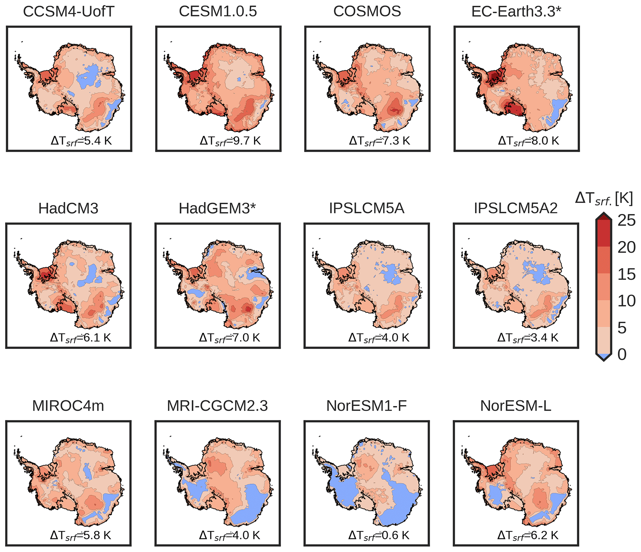
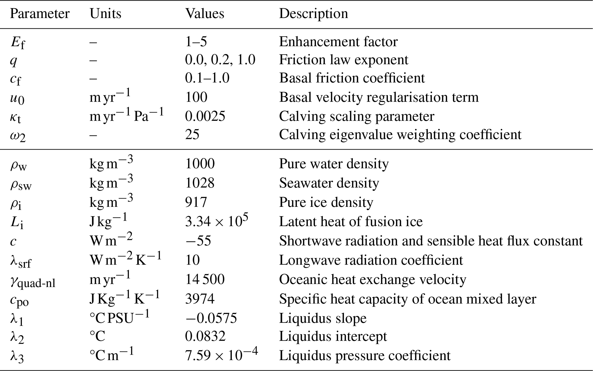
Figure 1Sea level temperature anomaly fields of the employed PlioMIP2 AOGCMs. Negative values (blue colours) represent a colder-than-PD surface temperature. Positive values (red colours) indicate a warmer-than-PD surface temperature. Numbers in the lower-right corner show the mean temperature anomaly inside the PD Antarctic domain (contour lines of the Antarctic grounding line and ice shelves). CMIP6 models are marked with an asterisk.
Atmospheric forcing
Ice sheet surface atmospheric temperatures and precipitation rates are obtained either from reanalysis or from climatic models. In order to investigate the response of the AIS to the mPWP climate, we use an anomaly method similar to Blasco et al. (2021), as follows:
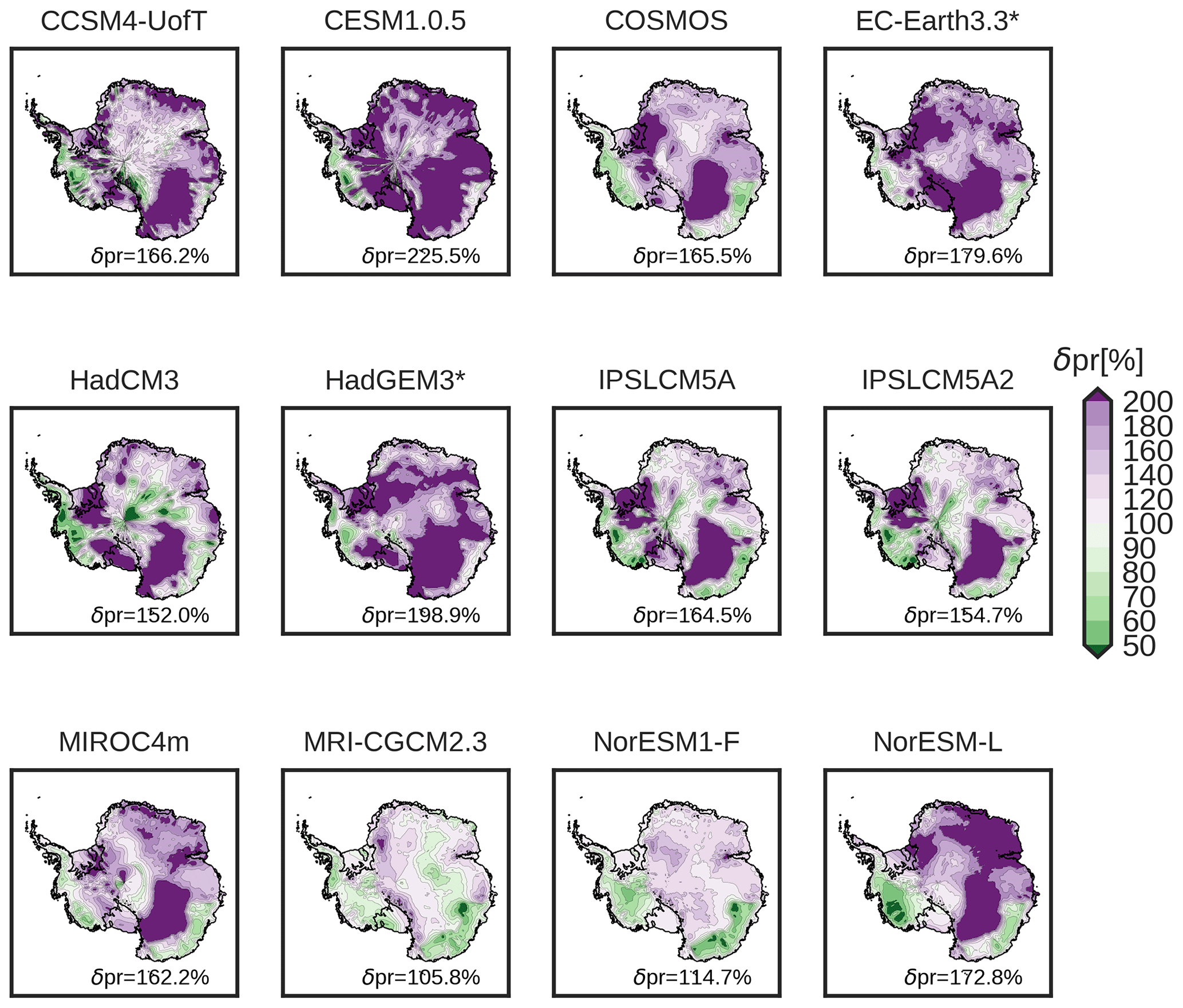
Figure 2Relative precipitation anomaly fields of the employed PlioMIP2 AOGCMs at sea level elevation. Values below 100 % (green colours) represent a drier climate (less precipitation than PD). Values above 100 % (purple colours) indicate more precipitation than in the PD. Numbers in the lower-right corner show the mean relative precipitation anomaly inside the PD Antarctic domain (contour lines of the Antarctic grounding line and ice shelves).
Here the subindex pd stands for present-day climate. These fields are obtained from the regional atmospheric climate model RACMO2.3 (Van Wessem et al., 2014) forced with the ERA-Interim reanalysis data (Dee et al., 2011). The temperature anomaly fields () and relative precipitation fields (δPmPWP) are computed between the Pliocene experiment with 400 ppmv CO2 and the pre-industrial control run using 280 ppmv CO2 from 12 different AOGCMs in the frame of PlioMIP2 (see Haywood et al., 2016, for more information on the experimental setup). In order to account for surface temperature and precipitation changes in elevation, a lapse rate correction factor Γ is applied, which is equal to 0.008 K m−1 for annual temperatures and to 0.0065 K m−1 for summer temperatures (Ritz et al., 1996; DeConto and Pollard, 2016; Quiquet et al., 2018; Albrecht et al., 2020).
where f is a precipitation change factor set to 0.05 °K−1 in the Clausius–Clapeyron relation. Note that in order to compute these fields, we needed to scale the PD and mPWP climatologies to PD sea level elevation using the same equations. PD climatologies are scaled with the surface elevation from RACMO2.3, whereas the mPWP climatologies are scaled with the surface elevations provided by the PlioMIP2 protocol. This ensures that surface changes, as well as any elevation bias from RACMO2.3 or PlioMIP2 fields, are taken into account in our model. Figures 1 and 2 show the anomaly fields from the 12 AOGCMs used in this study scaled to sea level elevation.
Figure 3Ocean thermal forcing temperature anomaly fields at the ice–ocean interface of the employed PlioMIP2 AOGCMs. Positive values (red colours) indicate a warmer bed–ocean temperature than in the PD. Grey colours indicate bedrock above sea level (based on PD topography) and, thus, with no ice–ocean interaction. The number in the lower-right corner shows the mean bed–temperature anomaly inside the PD Antarctic domain (contour lines of the Antarctic grounding line and ice shelves). Models in red are AOGCMs that did not provide any ocean field. The inferred ocean field was obtained as a mean of the atmospheric temperatures scaled by 0.25 (Taylor et al., 2012).
Ocean forcing
Here we use a quadratic local and non-local law following a similar approach to that of the ISMIP6 protocol (Jourdain et al., 2020). The quadratic local and non-local law includes not only local temperature changes but also the average over the ice shelf basin. This parameterisation accounts for the overturning circulation below the ice shelf cavities, which affects the total basal melt in a non-linear way (Favier et al., 2019). It reads as follows:
where γquad-nl represents the heat exchange velocity, ρsw and ρi are the ocean water and ice densities, respectively, cpo is the specific heat capacity of the ocean mixed layer; and Li is the latent heat of fusion of ice (Table 1). The freezing point temperature Tf at the ice shelf base is defined as
where zb represents the ice base elevation (negative below sea level), and the coefficients λ1, λ2, and λ3 are, respectively, the liquidus slope, intercept, and pressure coefficient (Table 1). Ocean temperature and salinity (Tf and Socn, respectively) are three-dimensional oceanic fields. PD fields are obtained from the World Ocean Database and extrapolated into the sub-shelf cavities following the ISMIP6 protocol (Jourdain et al., 2020). The mPWP fields are obtained from the AOGCMs outputs. A total of 4 of the 12 PlioMIP2 climate simulations, however, did not provide oceanic data. For those cases, a spatially homogeneous temperature anomaly field of one-fourth of the atmospheric anomaly was applied, following work by Golledge et al. (2015) and Taylor et al. (2012). The resulting thermal forcing anomaly field between the mPWP and PD is shown in Fig. 3.
Note that the AOGCMs do not provide any oceanic information under Antarctic ice shelf grid cells. Since that grid information is required to force our ice sheet model, we interpolate to that grid point using the value of the nearest neighbour at the same depth. Of course, applying other interpolation schemes – and increasing the spatial resolution of the grid – will change the oceanic conditions and lead to different final states. The ideal outcome would be to include ocean models that resolve the ocean circulation below the shelves, which is not the case for the PlioMIP2 ensemble. Jourdain et al. (2020) propose an extrapolation protocol, which is another possibility, but it would add another source of uncertainty. We used the nearest-neighbour interpolation scheme for simplicity, but the extrapolation of oceanic conditions inside ice shelf cavities is an ongoing challenge within the scientific community.
2.3 Experimental setup
Present-day spin-up
First, we perform an ensemble of 150 ice sheet simulations for the AIS with different dynamic configurations under steady PD climatic conditions using the PD forcing fields. The ice sheet dynamics, thermodynamics, and topography are allowed to evolve freely. This approach differs from other studies, where friction coefficients are optimised to simulate an AIS that is as close as possible to observations. Instead, we use the more general friction coefficients that vary, depending on the bedrock properties described above, since there is no a priori reason to believe that optimised friction coefficients for PD would have been the same for the mPWP. However, we do a test of experiments with optimised friction coefficient fields, which we mention in Sect. 4.
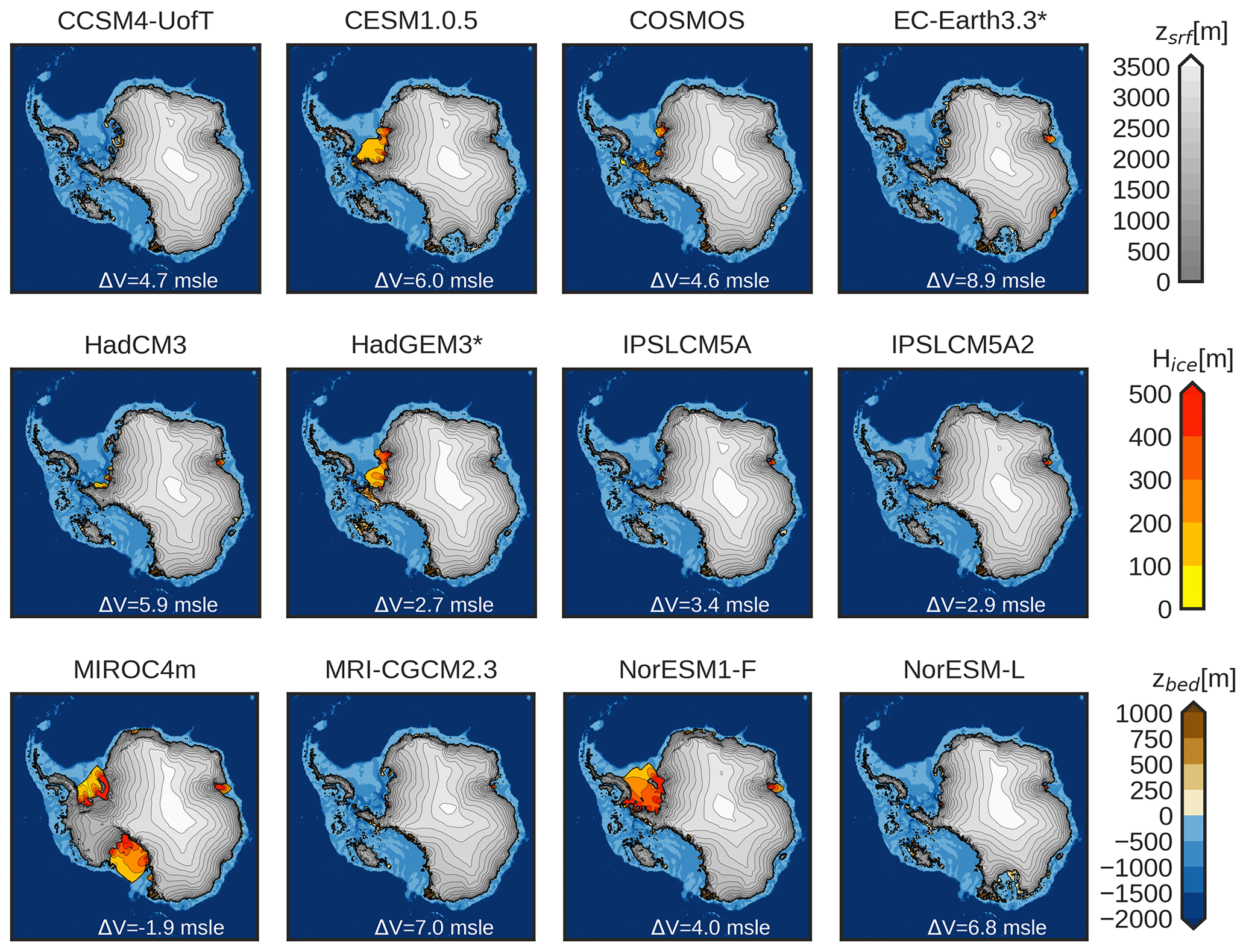
Figure 4Surface elevation (grey), floating ice thickness (red/orange/yellow), and bedrock elevation (brown/blue) of the simulation closest to the mean ice volume and ice extent of the ensemble for every AOGCM starting from PD bedrock conditions. The white number in the bottom corner represents the sea level rise with respect to the PD state.
We investigate uncertainty arising from three parameters that affect the ice dynamics: the exponent of the friction law q, the enhancement factor Ef, and the friction coefficient cf (Table 1). The friction exponent and coefficient affect the basal friction directly. In total, 10 values are chosen for the friction coefficient from 0.1 to 1.0 in steps of 0.1. Three values are chosen for the friction exponent: 0.0, 0.2, and 1.0. The enhancement factor is a typical arbitrary scalar introduced in the Arrhenius equation to approximate the effect of an anisotropic flow. It is chosen from 1 to 5 in steps of 1, following the values explored in Ma et al. (2010) (Table 1). The simulations are run for 100 kyr to ensure equilibration at the PD. Simulations are considered realistic if the simulated PD ice volume differs by less than 1 and if the grounded ice area differs by less than 2 % from observations from Morlighem et al. (2020). With these criteria, we simulate a PD state comparable to other ice sheet models (Seroussi et al., 2019). From our 150 ensemble members, only 31 simulations fulfil these conditions (Figs. S2–S4 in the Supplement).
Palaeo-simulations
The 31 selected model versions are then used to simulate mPWP conditions with forcing from the 12 different AOGCMs. This gives a total of 372 simulations. These simulations are initialised from the end of the respective PD simulation and forced under steady mPWP conditions until they reach a new equilibrated state; after 30 kyr, no significant changes are observed either in ice volume or in ice area (Figs. S2–S4). The background global sea level is set to 20 m above PD for all simulations, representative of the highest estimates. Assuming a fixed and stable mPWP climatic state is a simplification compared to reality, since the AIS ice volume and climate vary through time (Yan et al., 2016; DeConto and Pollard, 2016; Golledge et al., 2017). However, this approach allows us to make use of the PlioMIP AOGCM ensemble and to perform a straightforward comparison to gain insight into model sensitivities to climatic forcing.
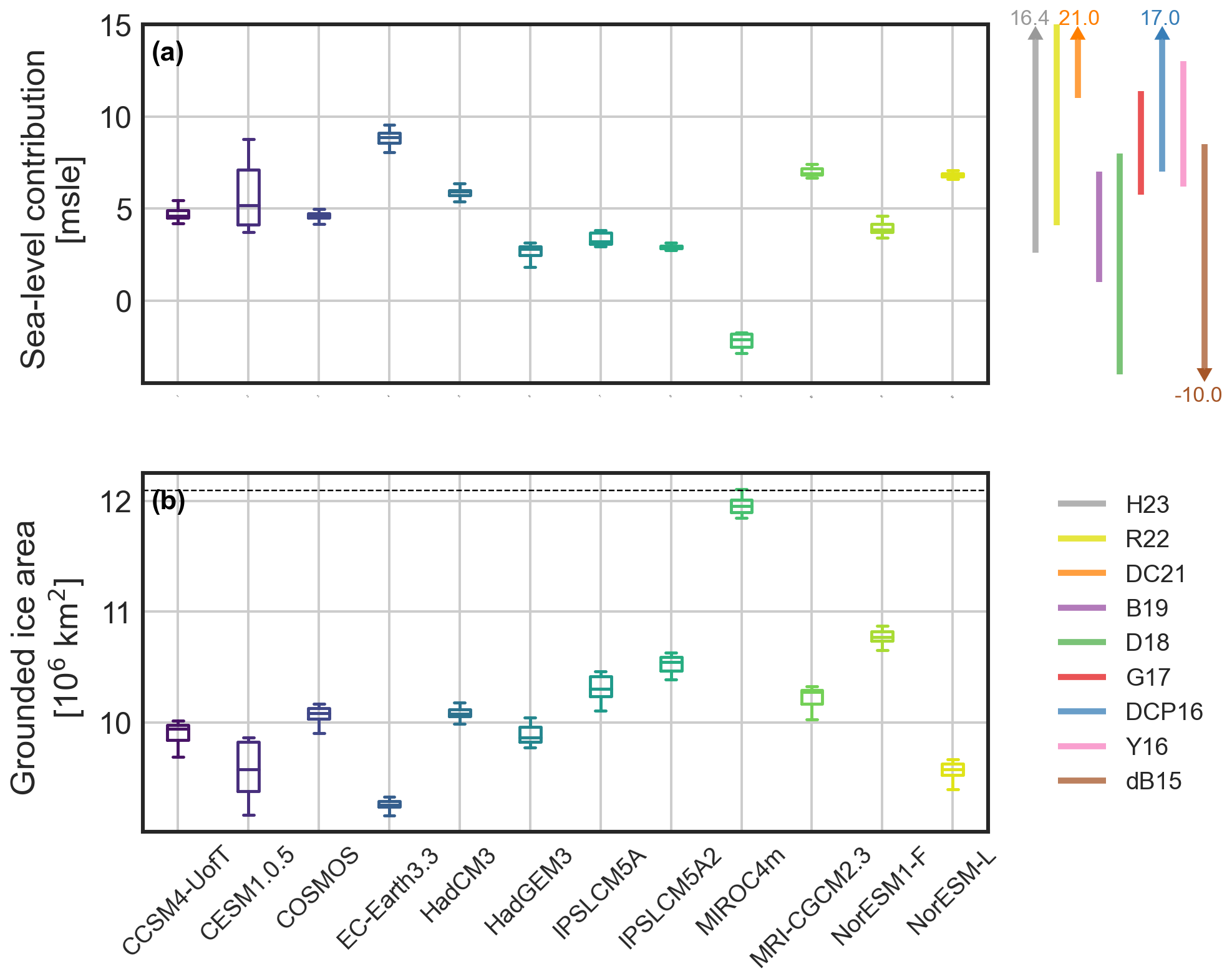
Figure 5Boxplot of the simulated (a) sea level contribution (positive/negative numbers indicate a lower/higher ice volume); and (b) grounded ice extent for every AOGCM. The error bars represent the lowest-/highest-simulated AIS state starting from PD conditions. Light shaded colours on the right show the sea level uncertainty ranges from the studies of de Boer et al. (2015) (brown), Yan et al. (2016) (pink), Golledge et al. (2017) (red), DeConto and Pollard (2016) (blue), Dolan et al. (2018) (green), Berends et al. (2019) (purple), DeConto et al. (2021) (orange), Richards et al. (2023) (yellow), and Hollyday et al. (2023) (grey). The dashed black line in panel (b) represents the PD grounded ice extent.
3.1 Ensemble simulations
The simulated ice volumes (in metres of sea level equivalent; ) and ice extent at equilibrium are shown in Figs. 4 and 5. All AOGCMs show a smaller AIS in terms of volume and extension, with one exception (MIROC4m). Based on sea level reconstructions, MIROC4m cannot be considered realistic; nonetheless, we will discuss the potential reason for this unexpected behaviour in the following sections. Over the remaining simulations, the simulated sea level contributions range from (HadGEM3; the uncertainty represents the interquartile range) to (EC-Earth3.3). Ice extent ranges from × 106 km2 (EC-Earth3.3) to × 106 km2 (NorESM1-F). For reference, the PD grounded extension lies around 12.3 × 10⁶ km2, while an extent of around 10 × 106 km2 represents a collapsed WAIS basin, and even lower numbers indicate a retreat of marine basins in the EAIS. Compared to previous modelling studies, our simulations are well within modelling estimates and in the lower range of AIS volume responses (Fig. 5a). No simulation reaches the lowest limit of 11 set by DeConto and Pollard (2016) (orange line), and just a few reach the lowest limit of 7 set by DeConto et al. (2021) (blue line). Results from Yan et al. (2016) (pink line) and Golledge et al. (2017) (red line) are closer to our upper limit, whereas those of Berends et al. (2019) (purple line) and Dolan et al. (2018) (green line) are inside the range of our simulations, and de Boer et al. (2015) (brown line) simulates a lower contribution. In comparison with the GIA (glacial isostatic adjustment) studies of Hollyday et al. (2023) (grey line) and Richards et al. (2023) (yellow line), our results show agreement within the lowest bounds.
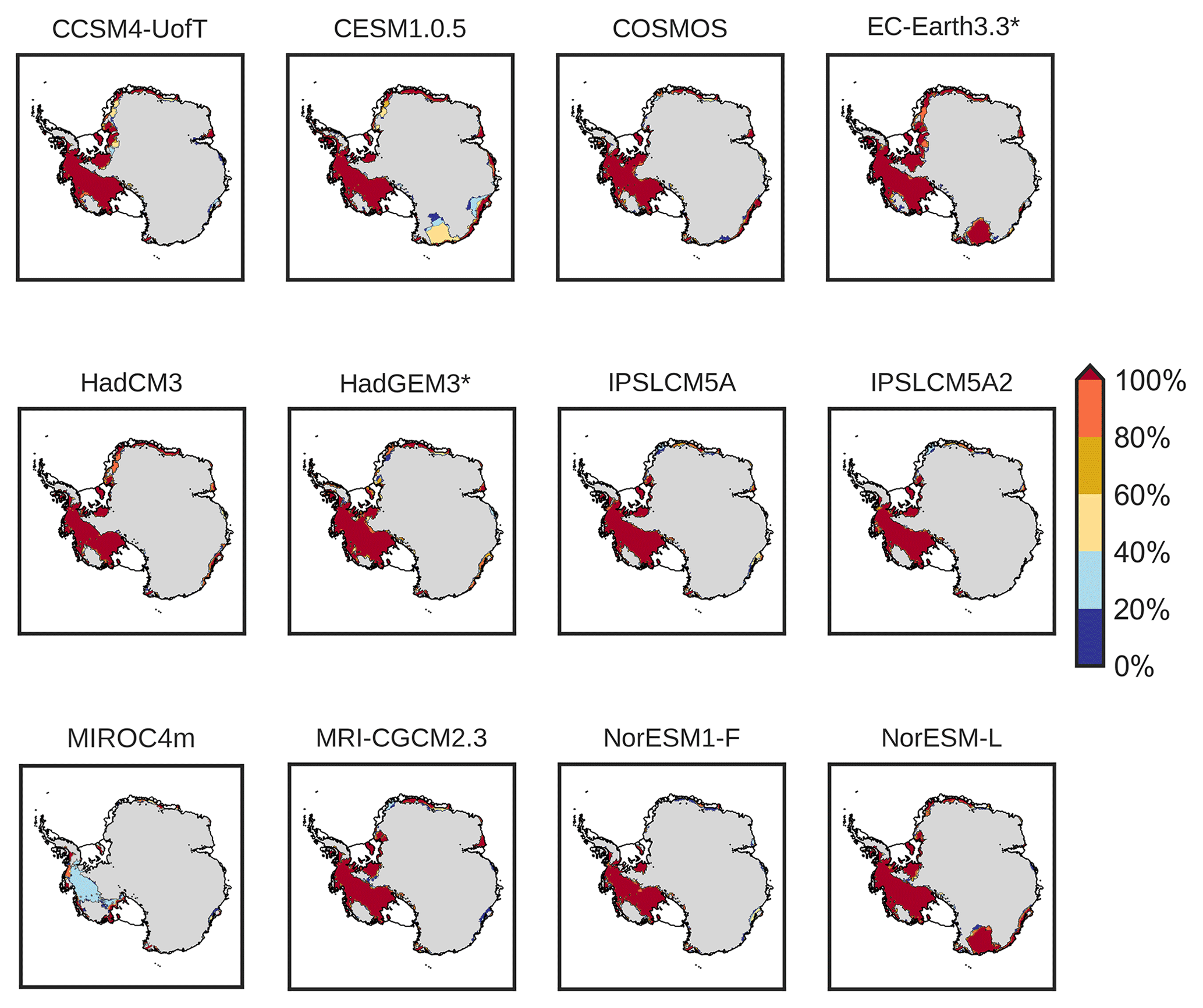
Figure 6Probability of ice collapse of the ensemble for every AOGCM. Red colours indicate 100 % probability of collapsed regions. Grey colours show grounded ice for all the ensemble simulations.
Figure 6 shows the ice collapse probability (here probabilities refer to empirical probabilities) for every AOGCM forcing applied (red is for a high probability of collapse; blue is for a low probability) and determined at each point as the fraction of simulations showing a collapse at that point from the ice sheet model ensemble. All cases (with the exception of MIROC4m) show a collapsed WAIS, though, in some cases, this retreat is more pronounced (COSMOS) than in other cases (NorESM1-F). In the Wilkes Basin, three AOGCM climates induce a retreat of the marine regions, though with different probabilities, namely low to medium in CESM1.0.5 and high in NorESM-L and EC-Earth3.3. The simulated sea level contribution of these cases is m s.l.e. (CESM1.0.5), m s.l.e. (EC-Earth3.3), and m s.l.e. (NorESM-L). Totten Glacier shows a slight retreat only for CESM1.0.5. Some regions of the EAIS close to the Filchner–Ronne Ice Shelf also retreat in some cases, especially for EC-Earth3.3 and CCSM4-UofT. Generally, ice sheets that are less extended lead to lower volumes, although this is not always the case (see simulations with HadGEM3 and MRI-CGCM2.3 forcing in Fig. 5).
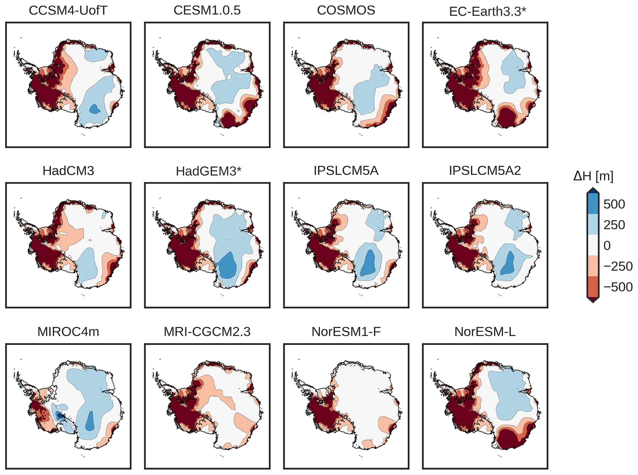
Figure 7Mean ice thickness anomaly between the mPWP state and the PD state. Positive/negative numbers (blue/red) represent a thicker/thinner ice column than the simulated PD.
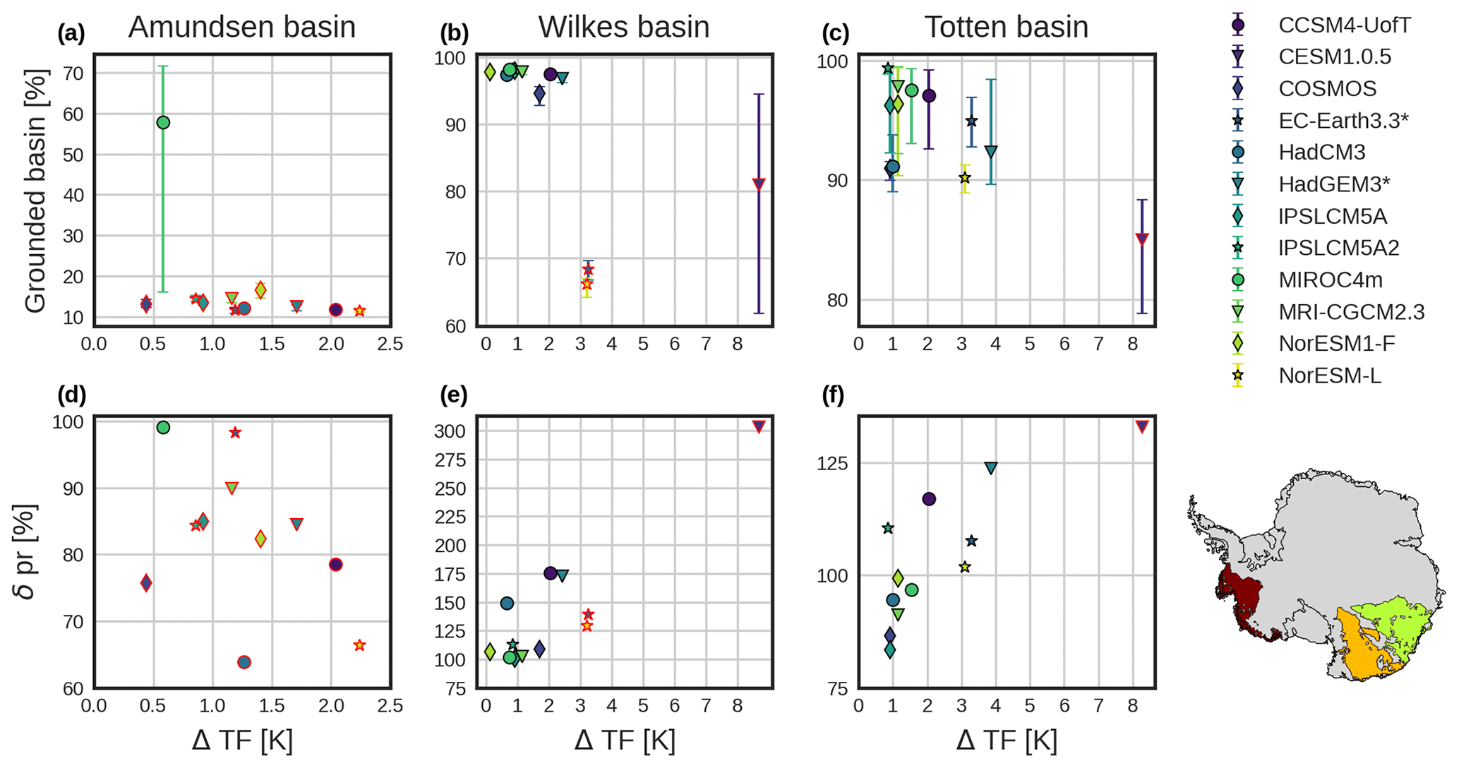
Figure 8Scatter plot of the grounded and simulated AIS ice area at the mPWP (in percentage of the marine basin, as in Fig. S1) with respect to the thermal forcing anomaly for (a) Amundsen Basin, (b) Wilkes Basin, and (c) Totten Glacier in the retreated regions (basins in Fig. S1). The error bars represent the lowest-/highest-simulated AIS state. (d–f) Same as panels (a)–(c) but for the relative precipitation anomaly relative to PD. Red borders represent either collapsed marine basins or ones that are more retreated than the rest of AOGCMs. In the bottom-right corner, the regions of interest are highlighted with dark red for Amundsen, orange for Wilkes, and green for Totten.
In order to assess the spatial origin of the mass loss for every AOGCM forcing, we plot the mean ice thickness anomaly between the simulated PlioMIP2 and PD state (Fig. 7). The ice thickness anomaly is nearly always negative (red colours) in the WAIS, since it has collapsed in that region. Even MIROC4m shows a negative thickness anomaly, though smaller in magnitude. In contrast, the EAIS presents more complex behaviour, depending on the AOGCM forcing. A warmer atmosphere enhances precipitation. Thus, the interior of the EAIS gains volume for some AOGCMs (CCSM4-UofT, HadGEM3, IPSLCM5A, and IPSLCM5A2). Nonetheless, sufficiently high ocean temperatures can induce a grounding line retreat in the Wilkes Basin. This is the case for simulations forced by CESM1.0.5, EC-Earth3.3, and NorESM-L. Simulations with COSMOS, NorESM1-F, and MRI-CGCM2.3 show a slightly negative anomaly in the coastal regions of EAIS. Although it does not propagate further inland, it seems to compensate for inland accumulation, leading to a value close to zero. This spread in the EAIS, and more specifically in the Wilkes Basin, points to an important role of the applied boundary conditions in the model response.
3.2 Tipping point analysis
Climatic forcing
We find in our study three potential sites prone to collapse, namely the WAIS through the Amundsen region; the Wilkes Basin; and, on a smaller scale, the Totten Glacier. We find that oceanic temperatures are the main forcing defining the ice extent of marine basins (Fig. 8). In the case of the Amundsen region (Fig. 8a), we observe that all simulations show a collapsed WAIS with one exception, the MIROC4m model. Though this result is not realistic in terms of sea level equivalent, as it points to an AIS bigger than today, it shows interesting results in terms of tipping points in the Amundsen Sea.
It is clear from Fig. 8a that even small temperature increases can lead to a collapse of the WAIS but that changes in precipitation can play a key role in low temperatures. Since we want to focus on the tipping point and thus the minimal oceanic temperature anomaly that leads to a collapse of the Amundsen Sea embayment, we focus on the four models that do not exceed 1 K of oceanic anomaly: COSMOS (0.44 K), IPSLCM5A (0.92 K), IPSLCM5A2 (0.86 K), and MIROC4m (0.58 K). Note that this anomaly has been computed for each basin (Fig. S1) at bedrock depth. By plotting the relative precipitation against the thermal forcing anomaly (Fig. 8d), we find that MIROC4m shows a relative precipitation anomaly close to PD values, whereas the IPSLCM5A and IPSLCM5A2 precipitation anomaly lies around 85 % of PD precipitation. Especially notable is the case of COSMOS, where the temperature anomaly is lower than MIROC4m – but so is the precipitation, at around 78 %. Thus, we see that a thermal forcing below 0.5 K can lead to a collapse of the WAIS if precipitation stays below 80 % of PD. Above the 1 K anomaly, we always find a collapsed WAIS even for precipitation rates close to PD (EC-Earth3.3). Nonetheless, it is important to mention that around 20 %–40 % (Fig. 6) of the MIROC4m simulations show a collapsed Amundsen embayment.
We redo the same analysis with the Wilkes Basin to investigate the tipping points that can lead to a collapse (Fig. 8b). Since the Wilkes Basin also lies on a retrograde bedrock, we assume that the oceanic thermal forcing is the main trigger. We find that the three AOGCMs that cause a collapse – EC-Earth3.3 (80 %–100 %), CESM1.0.5 (40 %–60 %), and NorESM-L (80 %–100 %) – simulate an oceanic anomaly above 3 K. Surprisingly, the CESM1.0.5 model, which has the highest thermal forcing anomaly, yields the highest uncertainty in the retreat (around 50 %; Fig. 6). This can be explained partially by the precipitation anomaly that is 3 times larger than PD rates (Fig. 8e). EC-Earth3.3 and NorESM-L have similar thermal forcing and precipitation anomalies (around 130 % of PD rates) and thus lead to similar results. Therefore, we conclude that a warming above 3 K can lead to an irreversible retreat of the Wilkes Basin. Nonetheless, this retreat can be somewhat mitigated by basin-wide enhanced precipitation rates, as seen in CESM1.0.5. This suggests an important role of ice dynamics. Hence, in the next section, we will analyse the potential role of ice dynamics for CESM1.0.5.
Finally we focus on Totten Glacier, since it also shows signs of potential instabilities for CESM1.0.5 (Fig. 6). When redoing the same analysis for that basin (Fig. 8c and f), we find that CESM1.0.5 simulates the lowest ice extent in Totten due to a thermal forcing anomaly above 8 K. The other models do not show a significant retreat (extension above 90 % of PD), even for thermal forcings close to 4 K. Thus, we conclude that for Totten Glacier, oceanic anomalies well above 4 K are needed to induce a retreat of the grounding line there.
Ice dynamics
Since we show that some basins collapse with certain probability for forcing from some AOGCMs, we focus our attention on the role of the ice dynamics in the ice retreat (Fig. S7 in the Supplement). We plot the three main parameters influencing the ice flow that we permuted in our simulations (enhancement factor Ef, friction law exponent q, and friction coefficient cf) for the two AOGCMs that showed a certain probability of collapse (CESM1.0.5 in the Wilkes and Totten Glacier basins and MIROC4m in the Amundsen Sea basin). For CESM1.0.5, we could not find any relationship between a Wilkes collapse and the dynamic configuration, except that lower enhancement factors simulated a more pronounced retreat than higher enhancement factors. On the other hand, for Totten Glacier, we find that simulations with higher enhancement factors (Ef = 5) never collapse, whereas simulations with lower values (Ef = 3) always collapse. Intermediate values (Ef = 4) show a regime with both states. Finally, no clear relationship is found for the MIROC4m model in the Amundsen Sea region, except that neither an enhancement factor of Ef = 3 nor a linear friction law (q=1) collapses.
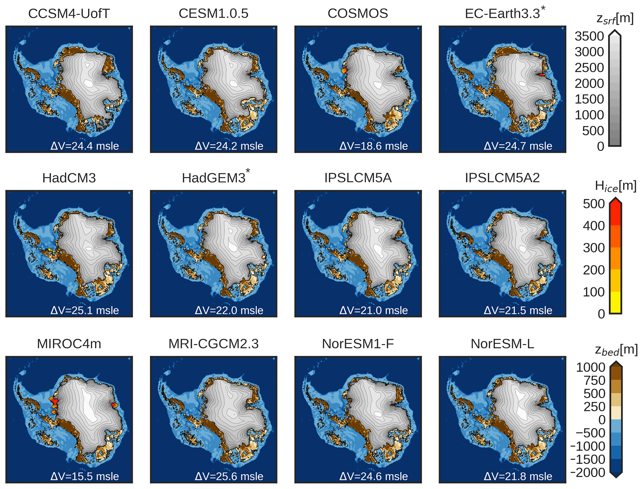
Figure 9Surface elevation (grey), floating ice thickness (red/orange/yellow), and bedrock elevation (brown/blue) of the simulation closest to the mean volume and extension of the ensemble for every AOGCM forcing, starting from PRISM4 boundary conditions. White numbers at the bottom represent the sea level rise with respect to the PD state.
3.3 Bedrock experiments
Some additional simulations were performed to test the effect of different topographic initial conditions on the final results. To avoid running the complete ensemble again, we took the ensemble parameters (cf, Ef, and q) which simulated the closest value to the mean for every AOGCM. We performed an additional set of simulations by imposing the Pliocene topography and ice thickness configuration from PRISM4 (Dowsett et al., 2016). PRISM4 surface elevation is illustrated in Fig. S6 in the Supplement. Figure 9 shows the surface elevation of the simulated AIS. In this case, all the simulations show a collapsed WAIS, as well as collapsed Wilkes and Totten Glacier basins. These results are more in agreement with the reconstructions used for the PRISM4 boundary conditions and the highest range of sea level estimates (sea level contributions from 15 to 25 m). Nonetheless, as we will discuss further, these results are biased towards a collapsed state, since regrowth on retrograde bedrock slopes is hampered. The existence of positive feedback mechanisms on marine retrograde bed slopes creates hysteresis behaviour.
4.1 Comparison with previous studies
We have presented a large ensemble forced with different mPWP climatologies. DeConto and Pollard (2016) and DeConto et al. (2021) also performed a large-ensemble analysis but only explored the relationships between ocean temperature and sub-ice-shelf melt rates, hydrofracturing, and maximum rates of marine-terminating ice cliff failure. Yan et al. (2016) used an ensemble to investigate parameters that affect the climatic conditions rather than ice dynamics. de Boer et al. (2015) and Dolan et al. (2018) include several climatic outputs and ice sheet models. Nonetheless, only one dynamic configuration was chosen for every ice sheet model. Here we aimed to consistently investigate the role of uncertainties in both the mPWP climatology by testing different AOGCMs, as well as ice dynamics.
In total, we simulate an Antarctic sea level contribution of less than 10 m if we start from PD conditions and use the PD topography (Fig. 5). Our results are in general agreement with many studies that start with PD initial conditions or evolve transiently towards the mPWP (de Boer et al., 2015; Yan et al., 2016; Golledge et al., 2017; Dolan et al., 2018; Berends et al., 2019). Our simulations differ greatly with the studies from DeConto and Pollard (2016) and DeConto et al. (2021), due to their inclusion of the MICI mechanism. Without MICI, those studies only show a collapse of the WAIS corresponding to 3 (Fig. S6a and b). However, it is worth mentioning that those studies applied an oceanic anomaly of only 2 K warming with respect to the PD at the mPWP. As shown in our study, with such a forcing we would not simulate a collapse of the Wilkes Basin or Totten Glacier retreat either, since at least a 3 K oceanic warming anomaly is needed. Furthermore, Crawford et al. (2021) showed that the applied rate of retreat for small cliffs was overestimated in DeConto and Pollard (2016). Other studies that achieve a collapse of the Wilkes Basin do it either by increasing oceanic temperatures (Yan et al., 2016; Golledge et al., 2017) or by adding melt at the grounding line (Golledge et al., 2017). Though not focused on the Pliocene, the ABUMIP (Antarctic BUttressing Model Intercomparison Project) experiments showed that the removal of ice shelves also leads to substantial ice loss in the Wilkes Basin for most models, showing that it is a highly vulnerable and uncertain region (Sun et al., 2020). Our results support a collapse of the Wilkes Basin for an oceanic anomaly of 3 K and a retreat of the Totten Glacier for an oceanic anomaly above 4 K. Nonetheless, high precipitation rates can hamper this retreat.
Since our Antarctic sea level contributions do not exceed 10 , our simulations do not support a global sea level contribution of more than 20 , as suggested by some reconstructions (Dumitru et al., 2019; Hearty et al., 2020). Nonetheless, recent work done with geodynamic models suggests a lower contribution in the mPWP than proxy data. These models simulate dynamic topographic changes on specific domains, namely the Patagonian region (Hollyday et al., 2023), the Australian region (Richards et al., 2023), and the Atlantic shoreline (Moucha and Ruetenik, 2017). The main advantage compared to proxy data is that processes that are difficult to assess on in situ measurements and have a big impact, such as geostatic uplift, can be considered. These results are then compared to proxy measurements from that region to assess the reality of their simulation. The new sea level estimates reduce the global sea level contribution significantly, i.e. 17.5 ± 6.4 (Hollyday et al., 2023), 16.0 ± 5.5 (Richards et al., 2023), and 15 (Moucha and Ruetenik, 2017). Assuming that Greenland was almost fully melted (∼ 7.4 ; Morlighem et al., 2017), with such a revised sea level reconstruction our results are inside the geological constraints if Wilkes Basin collapsed via high-oceanic thermal forcing or with low precipitation rates, as in MRI-CGCM2.3 (Table S1 in the Supplement). Richards et al. (2023) even go one step further and argue that the impact of the proposed MICI mechanism (DeConto and Pollard, 2016; DeConto et al., 2021) is overestimated. Though this is not within the scope of our work, these new results could highlight the need for new mPWP boundary conditions for AOGCMs and mainly a larger and thicker AIS than previously thought.
Although not focused on the mPWP, the study of Garbe et al. (2020) shows a threshold of the Wilkes Basin between 4 and 6 K of warming relative to pre-industrial levels for the atmosphere (equivalent to 1.5–2.5 K in the ocean in their study). The Totten Glacier retreats in their experiment with an atmospheric anomaly of 7 K (close to 3 K of oceanic warming). Nonetheless, as pointed out by their study, this threshold is highly sensitive to the structural model dependence.
In our study we do not find a clear distinction between our ensemble ice-sheet-dynamics-related parameters and the simulated ice extent or ice volume. Simulations forced with CESM1.0.5 simulate a slightly more retreated Totten Glacier for low enhancement factors (Fig. S7). We believe that this is a consequence of the simulated PD state rather than the modelled ice dynamics, since we did not use any constraint metrics in the EAIS. In the MIROC4m model, we find that a WAIS collapse is more likely to occur for high enhancement factors and low friction exponents, which promotes faster ice flow. In summary, although we observe some trends associated with the dynamic configuration for CESM1.0.5 and MIROC4m, no clear relationship can be found between the ice extent and the ensemble dynamical parameters. Our analysis allows us to assess the sea level uncertainties that arise from dynamical configuration and climatologies. We find that the climatologies yield a larger uncertainty (∼ 7 ) than that resulting from the dynamic configuration if parameters are constrained with PD observations. Dolan et al. (2018) obtain >10 between different ice sheet models, whereas we obtain <2 differences for simulations which are not close to tipping and up to 5 differences for CESM1.0.5 due to the proximity of Wilkes Basin to tipping or not (error bars in Fig. 5).
4.2 Forcing limitations
In our study, the transient character of the climate system was neglected for the sake of simplicity, as well as the poor knowledge on the transient forcing. Instead, we forced our model towards a steady mPWP state for an ensemble large enough to be statistically significant (more than 30 simulations) for 12 different mPWP conditions. This approach permits us to assess the Antarctic tipping points starting from PD conditions, as well as the impact of the uncertainty associated with state-of-the-art equilibrium mPWP climatic conditions. This experimental setup is in line with other studies, allowing for a similar comparison (Yan et al., 2016; DeConto and Pollard, 2016; DeConto et al., 2021). However, assuming a constant warming may lead to the overestimation of sea level contributions, since we impose a warm climate over longer timescales than for a transient experiment. For instance, as shown by Stap et al. (2022), the simulated Antarctic sea level contribution at the Miocene is lower for a transient forcing than for a constant forcing leading to steady state. To our knowledge, only one study has simulated the transient evolution of the AIS under the Pliocene (Berends et al., 2019). The transient climate forcing they used did not reach the necessary conditions to lead to a retreat in the Wilkes Basin and thus produced a relatively low sea level contribution (Fig. S6c).
It is important to mention that exceeding a tipping point does not mean that the ice sheet will collapse immediately but rather that it has reached the threshold temperature by which a retreat will be induced and further amplified by MISI. By plotting the one-dimensional evolution of the WAIS (Fig. S5 in the Supplement), we observe that the WAIS collapse usually occurs with a lag of 1000–5000 years from the application of the forcing. In some cases, it can reach up to 25 000 years. MISI not only is a matter of the oceanic temperature threshold but also depends on the grounding line position and the thermal forcing at this location, as well as precipitation. Thus, a transient character in the forcing could avoid certain ice collapses if the warming is not sufficiently long. Other factors, such as ice dynamics, could also delay (or accelerate) the grounding line position reaching a pronounced retrograde bedrock that leads to a full collapse of the WAIS or other marine basins.
Another limitation in our study is the initial topographic boundary condition. In order to overcome this problem, we performed additional experiments starting from the topography and ice sheet thickness reconstructed from PRISM4 conditions (Fig. 9). Our sea level estimates then shift towards the high-range estimates between 15–25 Such an experiment was performed in the studies of Dolan et al. (2018) and de Boer et al. (2015). Their results also show that starting from PRISM4 conditions leads to higher sea level contributions and a less extended AIS during the mPWP. This result is expected, since a smaller ice sheet has warmer temperatures due to the melt–elevation feedback, as captured in our experiments through an atmospheric lapse rate factor. In addition, growing back on a retrograde marine basin needs a strong decrease in ocean temperature due to the hysteresis behaviour of the ice sheet. Runs that are initialised with PRISM4 conditions show an Antarctic sea level estimate up to 20
The mPWP was preceded by a large global glaciation during Marine Isotope Stage M2, ca. 3.3 Ma (Rohling et al., 2014; Stap et al., 2016). During that period, the AIS evolved towards a modern-like configuration (Berends et al., 2019). Therefore, starting from PD initial conditions can help assess the realism of the simulated mPWP from the AOGCMs. Our model only simulates a retreat in the Wilkes Basin, supported by reconstructions, for 3 out of 12 AOGCM models.
Our forcing strategy, based on an anomaly snapshot method (i.e. one constant climatic snapshot from each AOGCM), ignores certain climate interactions that could be relevant to the system. We take into account the surface melt–elevation feedback by employing the aforementioned lapse rate factor and albedo–melt feedback within our ITM parameterisation. However, these interactions could be improved with a spatially varying lapse rate factor computed from AOGCM temperature and elevation data (Crow et al., 2024). Nonetheless, probably one of the most important feedbacks not considered here is the effect of freshwater flux release from the AIS into the Southern Ocean. Results from Sadai et al. (2020) show that accounting for Antarctic ice discharges increases subsurface Southern Ocean temperatures. However, Bintanja et al. (2015) showed that ice shelf melt leads to a cooling of the Southern Ocean and an expansion of sea ice area. This points to the need for a more profound understanding of ice–ocean-related processes within models.
A more sophisticated approach would include direct coupling between an AOGCM and our ice sheet model. However, besides more computational resources, this would require constraints not only on our ice sheet model parameters but also on those of the AOGCM. The work of Berends et al. (2019) is a good example of a coupled ice sheet model based on a matrix method. However, in order to run these simulations at global scales, one trade-off is a lower ice sheet resolution (40 km). This is a potential explanation for why they do not simulate a retreat in the East Antarctic region. Here we aim to obtain a more nuanced understanding of processes related to ice dynamics – in part through a higher spatial resolution (16 km).
Finally, additional sources of forcing uncertainties exist which have not been taken into account, such as geothermal heat flow or the Earth rheology. On the one hand, assessing the geothermal heat flow at the PD represents a source of uncertainty (Burton-Johnson et al., 2020); thus, its value during the mPWP represents a major unknown. Earth rheology in this study was considered homogeneous for the whole AIS based on the elastic lithosphere-relaxed asthenosphere method (Le Meur and Huybrechts, 1996). Our study did not focus on the role of GIA on our simulations; however, new model implementations are planned in future work with Yelmo with a new GIA model which includes lateral variability (Swierczek-Jereczek et al., 2023).
4.3 Model limitations
As shown by Pattyn et al. (2013), a high resolution is needed at the grounding line to simulate accurate grounding line migrations. Ice sheet models use different techniques at the grounding line to compensate for the coarse resolution, such as flux conditions (Schoof, 2007; Tsai et al., 2015) or scaling friction at the grounding line by the grounded ice fraction. In our study, we use the latter technique which has been shown to simulate realistic grounding line migrations on idealised domains (a thorough description is presented by Robinson et al., 2020). We also ensure that effective pressure, which enters the basal friction equation, tends to zero as the ice thickness approaches flotation (Leguy et al., 2014). Nonetheless, the grounding line representation remains a source of uncertainty that can strongly influence the retreat of marine-based glaciers prone to MISI.
Another source of uncertainty is the melting at the grounding line. Observations have established that the ocean-induced basal melting is highest close to the grounding line and decreases towards the ice shelf front (Adusumilli et al., 2020). Ice sheet models use different approaches which typically range from no ocean-induced melting to partial ocean-induced melting (Seroussi and Morlighem, 2018; Leguy et al., 2021). In many coarse-resolution ice sheet models (more than 2 km resolution at the grounding line), no melting is applied directly at the grounding line since it can lead to an overestimation of sub-shelf melting (Seroussi and Morlighem, 2018). Nonetheless, recent studies suggest that at a high spatial resolution, applying melting at the grounding line via a flotation criterion may be more accurate since it is less resolution-dependent (Leguy et al., 2021; Berends et al., 2023). This could suggest that our results correspond to a lower limit since no melting is applied at the grounding line in our experiments. We expect that by adding melting at the grounding line, the collapse of the Wilkes Basin would have been more likely for those AOGCM climates with lower-oceanic thermal forcing. Basal melting representation remains a fundamental source of uncertainty which needs further investigation.
A final source of uncertainty comes from the unknown basal conditions. Here we used a spatially constant friction coefficient scaled with the bedrock depth to favour more sliding at deeper bedrocks. Another common approach is to compute friction coefficients through an optimisation procedure aiming at minimising the errors in ice thickness with respect to observations (Lipscomb et al., 2019, 2021). Our simulations with a homogeneous friction coefficient produce satisfactory results in terms of RMSE of ice thickness and surface velocities that are comparable to those of other groups in the context of ISMIP6 (Fig. S3). Furthermore, there is no a priori reason to believe that optimised friction coefficients for PD would have been the same for the mPWP. Our approach has the benefit that basal friction adapts to changes in ice thickness and effective pressure as a result of changes in the mPWP boundary conditions with respect to the present day. Therefore, we believe that for our study, it is more beneficial to use a simple parameterisation, as done in other palaeo-studies (Quiquet et al., 2018), rather than optimised friction coefficients. A potential future improvement could be to include an active sediment mask to account for changes in erosion, which can change the bed roughness.
Here we investigated the AIS response to mPWP conditions to assess its sea level contribution during the mPWP and the potential tipping points that our ice sheet model exhibit under mPWP scenarios. A way to gain insight into tipping point behaviours of ice sheets would be to perform an intercomparison between different ice sheet models and analyse different sources of uncertainty, such as grounding line basal melt and basal friction at the grounding line or resolution, among others. In this study, we aimed to contribute to this discussion by testing dynamic sources of uncertainty in the Yelmo ice sheet model under different mPWP climatic forcings in the framework of the PlioMIP2 project. We have identified that the WAIS exhibits a tipping point for an oceanic warming of 0.5 K, as long as regional precipitation remains below that of PD. When the oceanic warming reaches 1 K anomaly, even precipitation similar to today's or higher is unable to prevent a MISI. In the Wilkes Basin, a retreat occurs when the oceanic warming reaches 3 K. However, we have observed that high precipitation, up to 3 times higher than today, can potentially prevent such a retreat. Additionally, we have found that the Totten Glacier can also retreat but only under high-oceanic warming conditions at least above the 4 K ocean temperature anomaly. In addition, we explored the initialisation of the model with an ice sheet thickness derived from PRISM4. This initialisation resulted in a lower AIS in terms of both ice volume and extent due to starting from already retreated marine basins. Consequently, the model initialised with the PRISM4 ice sheet thickness displayed persistent differences in the simulated AIS characteristics compared to other initialisations.
Finally, our mean simulated mPWP sea level contributions (relative to PD) for every AOGCM ranged from to , considering the whole ensemble starting from PD conditions, and 15.5 to 25.6 , when starting from PRISM4 conditions. If only the WAIS collapses, sea level contributions range from to If only the Wilkes Basin collapses, sea level contributions range from to The contributions starting from PD conditions are in agreement with geological constraints which do not exceed global sea level stands above 20 However, the collapse of the Wilkes Basin is a necessary condition in order to achieve Antarctic sea level rises above 7 Ultimately, the MICI mechanism is not a necessary condition for a collapse of the Wilkes Basin, since high-oceanic temperatures can also lead to such a collapse. Our results reinforce the hypothesis that crossing several Antarctic tipping points is necessary for large sea level high stands to be obtained at the mPWP.
Yelmo is maintained as a GitHub repository hosted at https://github.com/palma-ice/yelmo (Robinson et al., 2024) under licence no. GPL-3.0. Model documentation can be found at https://palma-ice.github.io/yelmo-docs/ (last access: 1 August 2024). The simulated mPWP states are available on Zenodo (https://doi.org/10.5281/zenodo.12742389, Blasco Navarro, 2024).
The supplement related to this article is available online at: https://doi.org/10.5194/cp-20-1919-2024-supplement.
JB carried out the simulations, analysed the results, and wrote the paper. All other co-authors contributed to designing the simulations, analysing the results, and writing the paper.
At least one of the (co-)authors is a member of the editorial board of Climate of the Past of the special issue “Icy landscapes of the past”. The peer-review process was guided by an independent editor, and the authors also have no other competing interests to declare.
Publisher's note: Copernicus Publications remains neutral with regard to jurisdictional claims made in the text, published maps, institutional affiliations, or any other geographical representation in this paper. While Copernicus Publications makes every effort to include appropriate place names, the final responsibility lies with the authors.
This article is part of the special issue “Icy landscapes of the past”. It is not associated with a conference.
We are grateful to the reviewer Tijn Berends and the anonymous reviewer, as well as the editor Lev Tarasov, for helpful comments which improved the final version of the paper.
This project is TiPES contribution no. 246. This project has received funding from the European Union’s Horizon 2020 research and innovation programme under grant no. 820970. Alexander Robinson received funding from the European Union (ERC, FORCLIMA; grant no. 101044247). This research has also been supported by the Spanish Ministry of Science and Innovation project MARINE (grant no. PID2020-117768RB-I00). Simulations were performed with Brigit, the high-performance computer (HPC) of the Campus of International Excellence of Moncloa, and funded by MECD and MICINN.
This paper was edited by Lev Tarasov and reviewed by Tijn Berends and one anonymous referee.
Adusumilli, S., Fricker, H. A., Medley, B., Padman, L., and Siegfried, M. R.: Interannual variations in meltwater input to the Southern Ocean from Antarctic ice shelves, Nat. Geosci., 13, 616–620, https://doi.org/10.1038/s41561-020-0616-z, 2020. a
Albrecht, T., Winkelmann, R., and Levermann, A.: Glacial-cycle simulations of the Antarctic Ice Sheet with the Parallel Ice Sheet Model (PISM) – Part 1: Boundary conditions and climatic forcing, The Cryosphere, 14, 599–632, https://doi.org/10.5194/tc-14-599-2020, 2020. a
Armstrong McKay, D. I., Staal, A., Abrams, J. F., Winkelmann, R., Sakschewski, B., Loriani, S., Fetzer, I., Cornell, S. E., Rockström, J., and Lenton, T. M.: Exceeding 1.5 °C global warming could trigger multiple climate tipping points, Science, 377, eabn7950, https://doi.org/10.1126/science.abn7950, 2022. a
Bassis, J., Berg, B., Crawford, A., and Benn, D.: Transition to marine ice cliff instability controlled by ice thickness gradients and velocity, Science, 372, 1342–1344, https://doi.org/10.1126/science.abf6271, 2021. a
Berends, C. J., de Boer, B., Dolan, A. M., Hill, D. J., and van de Wal, R. S. W.: Modelling ice sheet evolution and atmospheric CO2 during the Late Pliocene, Clim. Past, 15, 1603–1619, https://doi.org/10.5194/cp-15-1603-2019, 2019. a, b, c, d, e, f, g, h
Berends, C. J., Goelzer, H., Reerink, T. J., Stap, L. B., and van de Wal, R. S. W.: Benchmarking the vertically integrated ice-sheet model IMAU-ICE (version 2.0), Geosci. Model Dev., 15, 5667–5688, https://doi.org/10.5194/gmd-15-5667-2022, 2022. a
Berends, C. J., Stap, L. B., and van de Wal, R. S.: Strong impact of sub-shelf melt parameterisation on ice-sheet retreat in idealised and realistic Antarctic topography, J. Glaciol., 69, 1434–1448, https://doi.org/10.1017/jog.2023.33, 2023. a
Bertram, R. A., Wilson, D. J., van de Flierdt, T., McKay, R. M., Patterson, M. O., Jimenez-Espejo, F. J., Escutia, C., Duke, G. C., Taylor-Silva, B. I., and Riesselman, C. R.: Pliocene deglacial event timelines and the biogeochemical response offshore Wilkes Subglacial Basin, East Antarctica, Earth Planet. Sci. Lett., 494, 109–116, https://doi.org/10.1016/j.epsl.2018.04.054, 2018. a
Bintanja, R., Van Oldenborgh, G., and Katsman, C.: The effect of increased fresh water from Antarctic ice shelves on future trends in Antarctic sea ice, Ann. Glaciol., 56, 120–126, https://doi.org/10.3189/2015AoG69A001, 2015. a
Blasco Navarro, J.: Antarctic Tipping points triggered by the mid-Pliocene warm climate, Zenodo [data set], https://doi.org/10.5281/zenodo.12742389, 2024. a
Blasco, J., Alvarez-Solas, J., Robinson, A., and Montoya, M.: Exploring the impact of atmospheric forcing and basal drag on the Antarctic Ice Sheet under Last Glacial Maximum conditions, The Cryosphere, 15, 215–231, https://doi.org/10.5194/tc-15-215-2021, 2021. a, b
Burton-Johnson, A., Dziadek, R., and Martin, C.: Review article: Geothermal heat flow in Antarctica: current and future directions, The Cryosphere, 14, 3843–3873, https://doi.org/10.5194/tc-14-3843-2020, 2020. a
Crawford, A. J., Benn, D. I., Todd, J., Åström, J. A., Bassis, J. N., and Zwinger, T.: Marine ice-cliff instability modeling shows mixed-mode ice-cliff failure and yields calving rate parameterization, Nat. Commun., 12, 2701, https://doi.org/10.1038/s41467-021-23070-7, 2021. a, b, c
Crow, B. R., Tarasov, L., Schulz, M., and Prange, M.: Uncertainties originating from GCM downscaling and bias correction with application to the MIS-11c Greenland Ice Sheet, Clim. Past, 20, 281–296, https://doi.org/10.5194/cp-20-281-2024, 2024. a
Cuffey, K. M. and Paterson, W. S. B.: The physics of glaciers, Elsevier, ISBN 9780123694614, 2010. a
Davies, J. H.: Global map of solid Earth surface heat flow, Geochem., Geophy., Geosy., 14, 4608–4622, https://doi.org/10.1002/ggge.20271, 2013. a
de Boer, B., Dolan, A. M., Bernales, J., Gasson, E., Goelzer, H., Golledge, N. R., Sutter, J., Huybrechts, P., Lohmann, G., Rogozhina, I., Abe-Ouchi, A., Saito, F., and van de Wal, R. S. W.: Simulating the Antarctic ice sheet in the late-Pliocene warm period: PLISMIP-ANT, an ice-sheet model intercomparison project, The Cryosphere, 9, 881–903, https://doi.org/10.5194/tc-9-881-2015, 2015. a, b, c, d, e, f
De La Vega, E., Chalk, T. B., Wilson, P. A., Bysani, R. P., and Foster, G. L.: Atmospheric CO2 during the Mid-Piacenzian Warm Period and the M2 glaciation, Sci. Rep.-UK, 10, 1–8, https://doi.org/10.1038/s41598-020-67154-8, 2020. a
DeConto, R. M. and Pollard, D.: Contribution of Antarctica to past and future sea-level rise, Nature, 531, 591–597, https://doi.org/10.1038/nature17145, 2016. a, b, c, d, e, f, g, h, i, j, k
DeConto, R. M., Pollard, D., Alley, R. B., Velicogna, I., Gasson, E., Gomez, N., Sadai, S., Condron, A., Gilford, D. M., Ashe, E. L., Kopp, R. E., Li, D., and Dutton, A.: The Paris Climate Agreement and future sea-level rise from Antarctica, Nature, 593, 83–89, https://doi.org/10.1038/s41586-021-03427-0, 2021. a, b, c, d, e, f, g, h, i
Dee, D. P., Uppala, S. M., Simmons, A. J., Berrisford, P., Poli, P., Kobayashi, S., Andrae, U., Balmaseda, M. A., Balsamo, G., Bauer, P., Bechtold, P., Beljaars, A. C. M., van de Berg, L., Bidlot, J., Bormann, N., Delsol, C., Dragani, R., Fuentes, M., Geer, A. J., Haimberger, L., Healy, S. B., Hersbach, H., Hólm, E. V., Isaksen, L., Kållberg, P., Köhler, M., Matricardi, M., McNally, A. P., Monge-Sanz, B. M., Morcrette, J.-J., Park, B.-K., Peubey, C., de Rosnay, P., Tavolato, C., Thépaut, J.-N., and Vitart, F.: The ERA-Interim reanalysis: Configuration and performance of the data assimilation system, Q. J. Roy. Meteor. Soc., 137, 553–597, https://doi.org/10.1002/qj.828, 2011. a
Dolan, A. M., De Boer, B., Bernales, J., Hill, D. J., and Haywood, A. M.: High climate model dependency of Pliocene Antarctic ice-sheet predictions, Nat. Commun., 9, 2799, https://doi.org/10.1038/s41467-018-05179-4, 2018. a, b, c, d, e, f, g, h
Dowsett, H., Dolan, A., Rowley, D., Moucha, R., Forte, A. M., Mitrovica, J. X., Pound, M., Salzmann, U., Robinson, M., Chandler, M., Foley, K., and Haywood, A.: The PRISM4 (mid-Piacenzian) paleoenvironmental reconstruction, Clim. Past, 12, 1519–1538, https://doi.org/10.5194/cp-12-1519-2016, 2016. a
Dumitru, O. A., Austermann, J., Polyak, V. J., Fornós, J. J., Asmerom, Y., Ginés, J., Ginés, A., and Onac, B. P.: Constraints on global mean sea level during Pliocene warmth, Nature, 574, 233–236, https://doi.org/10.1038/s41586-019-1543-2, 2019. a, b
Edwards, T. L., Brandon, M. A., Durand, G., Edwards, N. R., Golledge, N. R., Holden, P. B., Nias, I. J., Payne, A. J., Ritz, C., and Wernecke, A.: Revisiting Antarctic ice loss due to marine ice-cliff instability, Nature, 566, 58–64, https://doi.org/10.1038/s41586-019-0901-4, 2019. a
Favier, L., Jourdain, N. C., Jenkins, A., Merino, N., Durand, G., Gagliardini, O., Gillet-Chaulet, F., and Mathiot, P.: Assessment of sub-shelf melting parameterisations using the ocean–ice-sheet coupled model NEMO(v3.6)–Elmer/Ice(v8.3), Geosci. Model Dev., 12, 2255–2283, https://doi.org/10.5194/gmd-12-2255-2019, 2019. a
Feldmann, J., Albrecht, T., Khroulev, C., Pattyn, F., and Levermann, A.: Resolution-dependent performance of grounding line motion in a shallow model compared with a full-Stokes model according to the MISMIP3d intercomparison, J. Glaciol., 60, 353–360, https://doi.org/10.3189/2014JoG13J093, 2014. a
Fischer, H., Meissner, K. J., Mix, A. C., Abram, N. J., Austermann, J., Brovkin, V., Capron, E., Colombaroli, D., Daniau, A.-L., Dyez, K. A., Felis, T., Finkelstein, S. A., Jaccard, S. L., McClymont, E. L., Rovere, A., Sutter, J., Wolff, E. W., Affolter, S., Bakker, P., Ballesteros-Cánovas, J. A., Barbante, C., Caley, T., Carlson, A. E., Churakova (Sidorova), O., Cortese, G., Cumming, B. F., Davis, B. A. S., de Vernal, A., Emile-Geay, J., Fritz, S. C., Gierz, P., Gottschalk, J., Holloway, M. D., Joos, F., Kucera, M., Loutre, M.-F., Lunt, D. J., Marcisz, K., Marlon, J. R., Martinez, P., Masson-Delmotte, V., Nehrbass-Ahles, C., Otto-Bliesner, B. L., Raible, C. C., Risebrobakken, B., Sánchez Goñi, M. F., Arrigo, J. S., Sarnthein, M., Sjolte, J., Stocker, T. F., Velasquez Alvárez, P. A., Tinner, W., Valdes, P. J., Vogel, H., Wanner, H., Yan, Q., Yu, Z., Ziegler, M., and Zhou, L.: Palaeoclimate constraints on the impact of 2 °C anthropogenic warming and beyond, Nat. Geosci., 11, 474–485, https://doi.org/10.1038/s41561-018-0146-0, 2018. a
Fox-Kemper, B., Hewitt, H., Xiao, C., Aðalgeirsdóttir, G., Drijfhout, S., Edwards, T., Golledge, N., Hemer, M., Kopp, R., Krinner, G., Mix, A., Notz, D., Nowicki, S., Nurhati, I., Ruiz, L., Sallée, J.-B., Slangen, A., and Yu, Y.: Ocean, Cryosphere and Sea Level Change, edited by: Masson-Delmotte, V., Zhai, P., Pirani, A., Connors, S. L., Péan, C., Berger, S., Caud, N., Chen, Y., Goldfarb, L., Gomis, M. I., Huang, M., Leitzell, K., Lonnoy, E., Matthews, J. B. R., Maycock, T. K., Waterfield, T., Yelekçi, O., Yu, R., and Zhou, B., 1211–1362, Cambridge University Press, Cambridge, United Kingdom and New York, NY, USA, https://doi.org/10.1017/9781009157896.011, 2021. a
Frederikse, T., Landerer, F., Caron, L., Adhikari, S., Parkes, D., Humphrey, V. W., Dangendorf, S., Hogarth, P., Zanna, L., Cheng, L., and Wu, Y.-H.: The causes of sea-level rise since 1900, Nature, 584, 393–397, https://doi.org/10.1038/s41586-020-2591-3, 2020. a
Fürst, J. J., Durand, G., Gillet-Chaulet, F., Tavard, L., Rankl, M., Braun, M., and Gagliardini, O.: The safety band of Antarctic ice shelves, Nat. Clim. Change, 6, 479–482, https://doi.org/10.1038/nclimate2912, 2016. a
Garbe, J., Albrecht, T., Levermann, A., Donges, J. F., and Winkelmann, R.: The hysteresis of the Antarctic ice sheet, Nature, 585, 538–544, https://doi.org/10.1038/s41586-020-2727-5, 2020. a, b, c, d
Goldberg, D. N.: A variationally derived, depth-integrated approximation to a higher-order glaciological flow model, J. Glaciol., 57, 157–170, https://doi.org/10.3189/002214311795306763, 2011. a
Golledge, N. R., Kowalewski, D. E., Naish, T. R., Levy, R. H., Fogwill, C. J., and Gasson, E. G.: The multi-millennial Antarctic commitment to future sea-level rise, Nature, 526, 421–425, https://doi.org/10.1038/nature15706, 2015. a
Golledge, N. R., Thomas, Z. A., Levy, R. H., Gasson, E. G. W., Naish, T. R., McKay, R. M., Kowalewski, D. E., and Fogwill, C. J.: Antarctic climate and ice-sheet configuration during the early Pliocene interglacial at 4.23 Ma, Clim. Past, 13, 959–975, https://doi.org/10.5194/cp-13-959-2017, 2017. a, b, c, d, e, f, g, h
Grant, G., Naish, T., Dunbar, G., Stocchi, P., Kominz, M., Kamp, P. J., Tapia, C., McKay, R., Levy, R., and Patterson, M.: The amplitude and origin of sea-level variability during the Pliocene epoch, Nature, 574, 237–241, https://doi.org/10.1038/s41586-019-1619-z, 2019. a
Guillermic, M., Misra, S., Eagle, R., and Tripati, A.: Atmospheric CO2 estimates for the Miocene to Pleistocene based on foraminiferal δ11B at Ocean Drilling Program Sites 806 and 807 in the Western Equatorial Pacific, Clim. Past, 18, 183–207, https://doi.org/10.5194/cp-18-183-2022, 2022. a
Haywood, A. M., Dowsett, H. J., Dolan, A. M., Rowley, D., Abe-Ouchi, A., Otto-Bliesner, B., Chandler, M. A., Hunter, S. J., Lunt, D. J., Pound, M., and Salzmann, U.: The Pliocene Model Intercomparison Project (PlioMIP) Phase 2: scientific objectives and experimental design, Clim. Past, 12, 663–675, https://doi.org/10.5194/cp-12-663-2016, 2016. a, b
Hearty, P., Rovere, A., Sandstrom, M., O'Leary, M., Roberts, D., and Raymo, M. E.: Pliocene–Pleistocene Stratigraphy and sea-level estimates, Republic of South Africa with implications for a 400 ppmv CO2 world, Paleoceanography and Paleoclimatology, 35, e2019PA003835, https://doi.org/10.1029/2019PA003835, 2020. a, b
Hollyday, A., Austermann, J., Lloyd, A., Hoggard, M., Richards, F., and Rovere, A.: A revised estimate of early Pliocene global mean sea level using geodynamic models of the Patagonian slab window, Geochem., Geophy., Geosy., 24, e2022GC010648, https://doi.org/10.1029/2022GC010648, 2023. a, b, c, d, e
Jourdain, N. C., Asay-Davis, X., Hattermann, T., Straneo, F., Seroussi, H., Little, C. M., and Nowicki, S.: A protocol for calculating basal melt rates in the ISMIP6 Antarctic ice sheet projections, The Cryosphere, 14, 3111–3134, https://doi.org/10.5194/tc-14-3111-2020, 2020. a, b, c
Le Meur, E. and Huybrechts, P.: A comparison of different ways of dealing with isostasy: examples from modelling the Antarctic ice sheet during the last glacial cycle, Ann. Glaciol., 23, 309–317, https://doi.org/10.3189/S0260305500013586, 1996. a, b
Leguy, G. R., Asay-Davis, X. S., and Lipscomb, W. H.: Parameterization of basal friction near grounding lines in a one-dimensional ice sheet model, The Cryosphere, 8, 1239–1259, https://doi.org/10.5194/tc-8-1239-2014, 2014. a, b
Leguy, G. R., Lipscomb, W. H., and Asay-Davis, X. S.: Marine ice sheet experiments with the Community Ice Sheet Model, The Cryosphere, 15, 3229–3253, https://doi.org/10.5194/tc-15-3229-2021, 2021. a, b, c
Lhermitte, S., Sun, S., Shuman, C., Wouters, B., Pattyn, F., Wuite, J., Berthier, E., and Nagler, T.: Damage accelerates ice shelf instability and mass loss in Amundsen Sea Embayment, P. Natl. Acad. Sci. USA, 117, 24735–24741, https://doi.org/10.1073/pnas.1912890117, 2020. a
Lipscomb, W. H., Price, S. F., Hoffman, M. J., Leguy, G. R., Bennett, A. R., Bradley, S. L., Evans, K. J., Fyke, J. G., Kennedy, J. H., Perego, M., Ranken, D. M., Sacks, W. J., Salinger, A. G., Vargo, L. J., and Worley, P. H.: Description and evaluation of the Community Ice Sheet Model (CISM) v2.1, Geosci. Model Dev., 12, 387–424, https://doi.org/10.5194/gmd-12-387-2019, 2019. a, b
Lipscomb, W. H., Leguy, G. R., Jourdain, N. C., Asay-Davis, X., Seroussi, H., and Nowicki, S.: ISMIP6-based projections of ocean-forced Antarctic Ice Sheet evolution using the Community Ice Sheet Model, The Cryosphere, 15, 633–661, https://doi.org/10.5194/tc-15-633-2021, 2021. a
Ma, Y., Gagliardini, O., Ritz, C., Gillet-Chaulet, F., Durand, G., and Montagnat, M.: Enhancement factors for grounded ice and ice shelves inferred from an anisotropic ice-flow model, J. Glaciol., 56, 805–812, https://doi.org/10.3189/002214310794457209, 2010. a
Morlighem, M., Williams, C. N., Rignot, E., An, L., Arndt, J. E., Bamber, J. L., Catania, G., Chauché, N., Dowdeswell, J. A., Dorschel, B., Fenty, I., Hogan, K., Howat, I., Hubbard, A., Jakobsson, M., Jordan, T. M., Kjeldsen, K. K., Millan, R., Mayer, L., Mouginot, J., Noël, B. P. Y., O'Cofaigh, C., Palmer, S., Rysgaard, S., Seroussi, H., Siegert, M. J., Slabon, P., Straneo, F., van den Broeke, M. R., Weinrebe, W., Wood, M., and Zinglersen, K. B.: BedMachine v3: Complete bed topography and ocean bathymetry mapping of Greenland from multibeam echo sounding combined with mass conservation, Geophys. Res. Lett., 44, 11–051, https://doi.org/10.1002/2017GL074954, 2017. a, b
Morlighem, M., Rignot, E., Binder, T., Blankenship, D., Drews, R., Eagles, G., Eisen, O., Ferraccioli, F., Forsberg, R., Fretwell, P., Goel, V., Greenbaum, J. S., Gudmundsson, H., Guo, J., Helm, V., Hofstede, C., Howat, I., Humbert, A., Jokat, W., Karlsson, N. B., Lee, W. S., Matsuoka, K., Millan, R., Mouginot, J., Paden, J., Pattyn, F., Roberts, J., Rosier, S., Ruppel, A., Seroussi, H., Smith, E. C., Steinhage, D., Sun, B., Broeke, M. R. v. d., Ommen, T. D. v., Wessem, M. v., and Young, D. A.: Deep glacial troughs and stabilizing ridges unveiled beneath the margins of the Antarctic ice sheet, Nat. Geosci., 13, 132–137, https://doi.org/10.1038/s41561-019-0510-8, 2020. a, b, c
Moucha, R. and Ruetenik, G. A.: Interplay between dynamic topography and flexure along the US Atlantic passive margin: Insights from landscape evolution modeling, Global Planet. Chang., 149, 72–78, https://doi.org/10.1016/j.gloplacha.2017.01.004, 2017. a, b, c, d
Patterson, M. O., McKay, R., Naish, T., Escutia, C., Jimenez-Espejo, F., Raymo, M., Meyers, S., Tauxe, L., and Brinkhuis, H.: Orbital forcing of the East Antarctic ice sheet during the Pliocene and Early Pleistocene, Nat. Geosci., 7, 841–847, https://doi.org/10.1038/NGEO2273, 2014. a
Pattyn, F., Perichon, L., Durand, G., Favier, L., Gagliardini, O., Hindmarsh, R. C., Zwinger, T., Albrecht, T., Cornford, S., Docquier, D., Furst, J., Goldberg, D., Gudmundsson, G. H., Humbert, A., Hutten, M., Huybrechts, P., Jouvet, G., Kleiner, T., Larour, E., Martin, D., Morlighem, M., Payne, A. J., Pollard, D., Ruckamp, M., Rybak, O., Seroussi, H., Thoma, M., and Wilkens, N.: Grounding-line migration in plan-view marine ice-sheet models: results of the ice2sea MISMIP3d intercomparison, J. Glaciol., 59, 410–422, https://doi.org/10.3189/2013JoG12J129, 2013. a, b
Pellicciotti, F., Brock, B., Strasser, U., Burlando, P., Funk, M., and Corripio, J.: An enhanced temperature-index glacier melt model including the shortwave radiation balance: development and testing for Haut Glacier d'Arolla, Switzerland, J. Glaciol., 51, 573–587, https://doi.org/10.3189/172756505781829124, 2005. a
Quiquet, A., Dumas, C., Ritz, C., Peyaud, V., and Roche, D. M.: The GRISLI ice sheet model (version 2.0): calibration and validation for multi-millennial changes of the Antarctic ice sheet, Geosci. Model Dev., 11, 5003–5025, https://doi.org/10.5194/gmd-11-5003-2018, 2018. a, b
Richards, F. D., Coulson, S., Hoggard, M., Austermann, J., Dyer, B., and Mitrovica, J. X.: Geodynamically corrected Pliocene shoreline elevations in Australia consistent with midrange projections of Antarctic ice loss, Science Advances, 9, eadg3035, https://doi.org/10.1126/sciadv.adg3035, 2023. a, b, c, d, e, f, g
Rignot, E., Jacobs, S., Mouginot, J., and Scheuchl, B.: Ice-shelf melting around Antarctica, Science, 341, 266–270, https://doi.org/10.1126/science.1235798, 2013. a
Ritz, C., Fabre, A., and Letréguilly, A.: Sensitivity of a Greenland ice sheet model to ice flow and ablation parameters: consequences for the evolution through the last climatic cycle, Clim. Dynam., 13, 11–23, https://doi.org/10.1007/s003820050149, 1996. a
Robel, A. A. and Banwell, A. F.: A speed limit on ice shelf collapse through hydrofracture, Geophys. Res. Lett., 46, 12092–12100, https://doi.org/10.1029/2019GL084397, 2019. a
Robinson, A., Calov, R., and Ganopolski, A.: An efficient regional energy-moisture balance model for simulation of the Greenland Ice Sheet response to climate change, The Cryosphere, 4, 129–144, https://doi.org/10.5194/tc-4-129-2010, 2010. a, b
Robinson, A., Alvarez-Solas, J., Montoya, M., Goelzer, H., Greve, R., and Ritz, C.: Description and validation of the ice-sheet model Yelmo (version 1.0), Geosci. Model Dev., 13, 2805–2823, https://doi.org/10.5194/gmd-13-2805-2020, 2020. a, b, c
Robinson, A., Goldberg, D., and Lipscomb, W. H.: A comparison of the stability and performance of depth-integrated ice-dynamics solvers, The Cryosphere, 16, 689–709, https://doi.org/10.5194/tc-16-689-2022, 2022. a
Robinson, A., Alvarez-Solas, J., Montoya, M., Goelzer, H., Greve, R., and Ritz, C.: Yelmo ice-sheet model code base, GitHub [code], https://github.com/palma-ice/yelmo, last access: 3 September 2024. a
Rohling, E., Foster, G. L., Grant, K., Marino, G., Roberts, A., Tamisiea, M. E., and Williams, F.: Sea-level and deep-sea-temperature variability over the past 5.3 million years, Nature, 508, 477–482, https://doi.org/10.1038/nature13230, 2014. a, b
Rohling, E. J., Hibbert, F. D., Grant, K. M., Galaasen, E. V., Irvalı, N., Kleiven, H. F., Marino, G., Ninnemann, U., Roberts, A. P., Rosenthal, Y., Schulz, H., Williams, F. H., and Yu, J.: Asynchronous Antarctic and Greenland ice-volume contributions to the last interglacial sea-level highstand, Nat. Commun., 10, 5040, https://doi.org/10.1038/s41467-019-12874-3, 2019. a
Sadai, S., Condron, A., DeConto, R., and Pollard, D.: Future climate response to Antarctic Ice Sheet melt caused by anthropogenic warming, Science Advances, 6, eaaz1169, https://doi.org/10.1126/sciadv.aaz1169, 2020. a
Schoof, C.: Ice sheet grounding line dynamics: Steady states, stability, and hysteresis, J. Geophys. Res.-Earth, 112, F03S28, https://doi.org/10.1029/2006JF000664, 2007. a, b
Seroussi, H. and Morlighem, M.: Representation of basal melting at the grounding line in ice flow models, The Cryosphere, 12, 3085–3096, https://doi.org/10.5194/tc-12-3085-2018, 2018. a, b, c
Seroussi, H., Nowicki, S., Simon, E., Abe-Ouchi, A., Albrecht, T., Brondex, J., Cornford, S., Dumas, C., Gillet-Chaulet, F., Goelzer, H., Golledge, N. R., Gregory, J. M., Greve, R., Hoffman, M. J., Humbert, A., Huybrechts, P., Kleiner, T., Larour, E., Leguy, G., Lipscomb, W. H., Lowry, D., Mengel, M., Morlighem, M., Pattyn, F., Payne, A. J., Pollard, D., Price, S. F., Quiquet, A., Reerink, T. J., Reese, R., Rodehacke, C. B., Schlegel, N.-J., Shepherd, A., Sun, S., Sutter, J., Van Breedam, J., van de Wal, R. S. W., Winkelmann, R., and Zhang, T.: initMIP-Antarctica: an ice sheet model initialization experiment of ISMIP6, The Cryosphere, 13, 1441–1471, https://doi.org/10.5194/tc-13-1441-2019, 2019. a
Seroussi, H., Nowicki, S., Payne, A. J., Goelzer, H., Lipscomb, W. H., Abe-Ouchi, A., Agosta, C., Albrecht, T., Asay-Davis, X., Barthel, A., Calov, R., Cullather, R., Dumas, C., Galton-Fenzi, B. K., Gladstone, R., Golledge, N. R., Gregory, J. M., Greve, R., Hattermann, T., Hoffman, M. J., Humbert, A., Huybrechts, P., Jourdain, N. C., Kleiner, T., Larour, E., Leguy, G. R., Lowry, D. P., Little, C. M., Morlighem, M., Pattyn, F., Pelle, T., Price, S. F., Quiquet, A., Reese, R., Schlegel, N.-J., Shepherd, A., Simon, E., Smith, R. S., Straneo, F., Sun, S., Trusel, L. D., Van Breedam, J., van de Wal, R. S. W., Winkelmann, R., Zhao, C., Zhang, T., and Zwinger, T.: ISMIP6 Antarctica: a multi-model ensemble of the Antarctic ice sheet evolution over the 21st century, The Cryosphere, 14, 3033–3070, https://doi.org/10.5194/tc-14-3033-2020, 2020. a
Shakun, J. D., Corbett, L. B., Bierman, P. R., Underwood, K., Rizzo, D. M., Zimmerman, S. R., Caffee, M. W., Naish, T., Golledge, N. R., and Hay, C. C.: Minimal East Antarctic Ice Sheet retreat onto land during the past eight million years, Nature, 558, 284–287, https://doi.org/10.1038/s41586-018-0155-6, 2018. a
Stap, L. B., de Boer, B., Ziegler, M., Bintanja, R., Lourens, L. J., and van de Wal, R. S.: CO2 over the past 5 million years: Continuous simulation and new δ11B-based proxy data, Earth Planet. Sci. Lett., 439, 1–10, https://doi.org/10.1016/j.epsl.2016.01.022, 2016. a
Stap, L. B., Berends, C. J., Scherrenberg, M. D. W., van de Wal, R. S. W., and Gasson, E. G. W.: Net effect of ice-sheet–atmosphere interactions reduces simulated transient Miocene Antarctic ice-sheet variability, The Cryosphere, 16, 1315–1332, https://doi.org/10.5194/tc-16-1315-2022, 2022. a
Sun, S., Pattyn, F., Simon, E. G., Albrecht, T., Cornford, S., Calov, R., Dumas, C., Gillet-Chaulet, F., Goelzer, H., Golledge, N. R., Greve, R., Hoffman, M. J., Humbert, A., Kazmierczak, E., Kleiner, T., Leguy, G. R., Lipscomb, W. H., Martin, D., Morlighem, M., Nowicki, S., Pollard, D., Price, S., Quiquet, A., Seroussi, H., Schlemm, T., Sutter, J., van der Wal, R. S. W., Winkelmann, R., and Zhang, T.: Antarctic ice sheet response to sudden and sustained ice-shelf collapse (ABUMIP), J. Glaciol., 66, 891–904, https://doi.org/10.1017/jog.2020.67, 2020. a, b
Sutter, J., Gierz, P., Grosfeld, K., Thoma, M., and Lohmann, G.: Ocean temperature thresholds for last interglacial West Antarctic Ice Sheet collapse, Geophys. Res. Lett., 43, 2675–2682, https://doi.org/10.1002/2016GL067818, 2016. a
Swierczek-Jereczek, J., Montoya, M., Latychev, K., Robinson, A., Alvarez-Solas, J., and Mitrovica, J.: FastIsostasy v1.0 – An accelerated regional GIA model accounting for the lateral variability of the solid Earth, EGUsphere [preprint], https://doi.org/10.5194/egusphere-2023-2869, 2023. a
Taylor, K. E., Stouffer, R. J., and Meehl, G. A.: An overview of CMIP5 and the experiment design, B. Am. Meteorol. Soc., 93, 485–498, https://doi.org/10.1175/BAMS-D-11-00094.1, 2012. a, b
Tsai, V. C., Stewart, A. L., and Thompson, A. F.: Marine ice-sheet profiles and stability under Coulomb basal conditions, J. Glaciol., 61, 205–215, https://doi.org/10.3189/2015JoG14J221, 2015. a
van de Wal, R. S. W., Nicholls, R. J., Behar, D., McInnes, K., Stammer, D., Lowe, J. A., Church, J. A., DeConto, R., Fettweis, X., Goelzer, H., Haasnoot, M., Haigh, I. D., Hinkel, J., Horton, B. P., James, T. S., Jenkins, A., LeCozannet, G., Levermann, A., Lipscomb, W. H., Marzeion, B., Pattyn, F., Payne, A. J., Pfeffer, W. T., Price, S. F., Seroussi, H., Sun, S., Veatch, W., and White, K.: A High-End Estimate of Sea Level Rise for Practitioners, Earths Future, 10, e2022EF002751, https://doi.org/10.1029/2022EF002751, 2022. a
Van Den Berg, J., van de Wal, R., and Oerlemans, H.: A mass balance model for the Eurasian Ice Sheet for the last 120,000 years, Global Planet. Chang., 61, 194–208, https://doi.org/10.1016/j.gloplacha.2007.08.015, 2008. a
Van Wessem, J., Reijmer, C., Morlighem, M., Mouginot, J., Rignot, E., Medley, B., Joughin, I., Wouters, B., Depoorter, M., Bamber, J., Lenaerts, J., van de Berg, W., van den Broeke, M., and van Meijgaard, E.: Improved representation of East Antarctic surface mass balance in a regional atmospheric climate model, J. Glaciol., 60, 761–770, https://doi.org/10.3189/2014JoG14J051, 2014. a
Yan, Q., Zhang, Z., and Wang, H.: Investigating uncertainty in the simulation of the Antarctic ice sheet during the mid-Piacenzian, J. Geophys. Res.-Atmos., 121, 1559–1574, https://doi.org/10.1002/2015JD023900, 2016. a, b, c, d, e, f, g, h, i
Zoet, L. K. and Iverson, N. R.: A slip law for glaciers on deformable beds, Science, 368, 76–78, https://doi.org/10.1126/science.aaz1183, 2020. a