Relative importance of the mechanisms triggering the Eurasian ice sheet deglaciation in the GRISLI2.0 ice sheet model

The last deglaciation (21 to 8 ka) of the Eurasian ice sheet (EIS) is thought to have been responsible for a sea level rise of about 20 m. While many studies have examined the timing and rate of the EIS retreat during this period, many questions remain about the key processes that triggered the EIS deglaciation 21 kyr ago. Due to its large marine-based parts in the Barents–Kara (BKIS) and British Isles sectors, the BKIS is often considered to be a potential analogue of the current West Antarctic ice sheet (WAIS). Identifying the mechanisms that drove the EIS evolution might provide a better understanding of the processes at play in the West Antarctic destabilization. To investigate the relative impact of key drivers on the EIS destabilization, we used the three-dimensional ice sheet model GRISLI (GRenoble Ice Shelf and Land Ice) (version 2.0) forced by climatic fields from five Paleoclimate Modelling Intercomparison Project phases 3 and 4 (PMIP3, PMIP4) Last Glacial Maximum (LGM) simulations. In this study, we performed sensitivity experiments to test the response of the simulated Eurasian ice sheets to surface climate, oceanic temperatures (and thus basal melting under floating ice tongues), and sea level perturbations. Our results highlight that the EIS retreat simulated with the GRISLI model is primarily triggered by atmospheric warming. Increased atmospheric temperatures further amplify the sensitivity of the ice sheets to sub-shelf melting. These results contradict those of previous modelling studies mentioning the central role of basal melting on the deglaciation of the marine-based Barents–Kara ice sheet. However, we argue that the differences with previous works are mainly related to differences in the methodology followed to generate the initial LGM ice sheet. Due to the strong sensitivity of EIS to the atmospheric forcing highlighted with the GRISLI model and the limited extent of the confined ice shelves during the LGM, we conclude by questioning the analogy between EIS and the current WAIS. However, because of the expected rise in atmospheric temperatures, the risk of hydrofracturing is increasing and could ultimately put the WAIS in a configuration similar to the past Eurasian ice sheet.

1 Introduction

During the Last Glacial Maximum (LGM; 26–19 ka), the Eurasian ice complex was formed by the coalescence of three distinct ice sheets covering the British Isles, Fennoscandia, and the Barents and Kara seas. While the Fennoscandian ice sheet (FIS) was mostly grounded on the bedrock, the British Isles (BIIS) and Barents–Kara (BKIS) were mostly lying below sea level (Fig. 1).

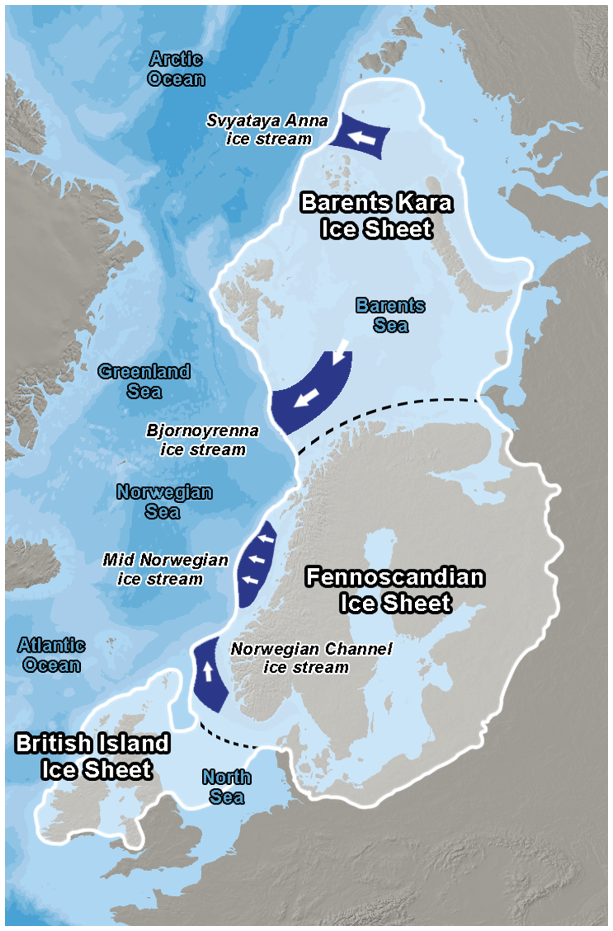
Figure 1 Map of the Eurasian ice sheet at the LGM. The white line is the most credible ice extent of the Eurasian ice sheet at the LGM, according to the DATED-1 compilation (Hughes et al., 2016). Dark blue shaded areas correspond to the location of the main ice streams (Dowdeswell et al., 2016; Stokes, 2001), and dotted black lines are delimitations between the Fennoscandian, the Barents–Kara, and the British Isles ice sheets.

The Eurasian ice sheet (EIS) was influenced by various climate regimes, with large differences between the western and eastern edges. Due to heat and moisture sources from the North Atlantic current, the British Isles and western Scandinavia were dominated by relatively warm and wet conditions, contrasting with the more continental and drier climate in the eastern part of the EIS (Tierney et al., 2020). These various climatic influences prevailing over the three different ice sheets forming the Eurasian ice complex may have resulted in different responses to variations in atmospheric and oceanic conditions. Over the last decade, an active field of research has developed to identify the mechanisms behind the retreat of the Eurasian ice sheet during the last deglaciation, although no clear consensus has yet been reached. According to the recent study of Sejrup et al. (2022), the onset of the Northern Hemisphere deglaciation was primarily triggered by summer ablation resulting from increased summer insolation at 65^∘ N and thus by changes in surface mass balance (SMB), defined as the difference between snow/ice accumulation and ablation.

On the other hand, studies based on modelling approaches suggest that the retreat of marine-based ice sheets could be driven by dynamical processes triggered by the melting of ice shelves (Pattyn, 2018). In fact, the relationship between oceanic temperatures and ice sheet mass balance has been confirmed and widely documented for the present-day West Antarctic ice sheet (WAIS). In particular, it has been shown that ocean warming plays a crucial role in accelerating Antarctic mass loss by enhancing basal melting and ice shelf thinning (Pritchard et al., 2012; Konrad et al., 2018; Pattyn, 2018; Rignot et al., 2019). This process may trigger marine ice sheet instability when the bedrock is sloping towards the ice sheet interior. This instability translates into a sustained retreat of the grounding line and a significant glacier acceleration (Schoof, 2012). As large parts of BIIS and BKIS are marine based, their evolution could be driven by sub-shelf melting and potentially by the subsequent marine ice sheet instability. Based on the analysis of benthic and planktic foraminiferal assemblages, ice-rafted debris, and radiocarbon dating, Rasmussen and Thomsen (2021) showed that the retreat of the ice in the Svalbard–Barents sector not only followed the deglacial oceanic but also atmospheric, temperature changes. Relying on a first-order thermomechanical ice sheet model constrained by a variety of geomorphological, geophysical, and geochronological data, Patton et al. (2017) found that the BIIS receded quite quickly in response to moderate increases in surface temperature. In contrast, the BKIS was rather affected by a combination of reduced precipitation and increased rates of iceberg calving. Other modelling studies have attempted to simulate the dynamics of the EIS during the Last Glacial Period and the last deglaciation with the objective of better understanding the evolution of the ice sheet (Petrini et al., 2020; Alvarez-Solas et al., 2019). In a way that is similar to what is currently observed in West Antarctica, they suggest that large EIS variations are primarily due to the warming of the Atlantic Ocean leading to increased basal melting in the vicinity of the grounding line (Petrini et al., 2020; Alvarez-Solas et al., 2019). However, the models on which these studies are based have no specific treatment for computing ice velocities at the grounding line, making their representation of the grounding line migration questionable.

Because of the diversity of mechanisms that may have influenced the evolution of the three Eurasian ice sheets, the Eurasian ice complex is an interesting case study to investigate the different mechanisms responsible for the ice sheet retreat. As both BKIS and BIIS are marine based (Svendsen et al., 2004; Gandy et al., 2018, 2021), they are likely to be more sensitive to oceanic temperature variations. Special attention can be given to BKIS because it has often been considered to be a potential analogue of the present-day WAIS (Gudlaugsson et al., 2017; Andreassen and Winsborrow, 2009; Mercer, 1970), due to common features such as the ice volume and a bedrock largely grounded below sea level with an upstream deepening (Amante, 2009). As a result, in-depth investigations of the BKIS behaviour at the LGM can help us to better understand the present-day changes and future evolution of West Antarctica.

This wide range of hypotheses regarding the different processes responsible for the EIS destabilization (i.e. atmospheric climate, oceanic climate, or both) confirms that there are still a lot of unknowns in the EIS dynamics during the last deglaciation and that the debate is not closed. Progress has been made in ice sheet modelling with the development of new-generation models computing the full Stokes flow equations. For example, with a refined model resolution near the grounding line, Gandy et al. (2018, 2021) have quantified the impact of oceanic temperatures on the grounding line dynamics and investigated the potential occurrence and effect of the marine ice sheet instability. However, as the computation time is considerably increased, they focus only on specific sectors (i.e. North Sea) and thus do not consider the impact of the other interconnected ice sheets.

In this paper, we present simulations of the entire Eurasian ice complex during the LGM using the three-dimensional GRISLI2.0 (GRenoble Ice Shelf and Land Ice) ice sheet model (Quiquet et al., 2018). GRISLI2.0 includes an explicit calculation of the ice flux at the grounding line derived from the analytical formulation provided by Tsai and Gudmundsson (2015), which is expected to account for the representation of the marine ice sheet instability. Our ultimate objective is not to reproduce the exact timing of the last deglaciation of the EIS but rather to explore the sensitivity of EIS to various perturbations using the GRISLI ice model.

Starting from its LGM geometry, we investigate the EIS sensitivity to perturbations of surface air temperature, precipitation rate, basal melting, and sea level to better understand their relative contribution to the EIS destabilization. In this work, the GRISLI2.0 ice sheet model was forced by a panel of 10 different climates from the Paleoclimate Modelling Intercomparison Project (PMIP) database (Abe-Ouchi et al., 2015; Kageyama et al., 2021).

The paper is organized as follows. Section 2 provides a description of the basic equations of the GRISLI2.0 ice sheet model. It also includes a presentation of the climate forcing and the experimental set-up of the LGM and sensitivity experiments. Section 3 compares our different reconstructions of the EIS at the LGM. The results of the sensitivity experiments are presented in Sect. 4 and discussed in Sect. 5. Concluding remarks are given in Sect. 6.

2 Model description and experimental set-up

2.1 The GRISLI ice sheet model

In this study, we use the 3D thermomechanical ice sheet model GRISLI2.0 (referred hereafter to as GRISLI) run on a Cartesian grid with a horizontal resolution of 20 km × 20 km, corresponding to 177×257 grid points.

This ice sheet model was initially built to study the Antarctic ice sheet behaviour during glacial–interglacial cycles (Ritz et al., 2001). It was then adapted to the Northern Hemisphere ice sheets (e.g. Peyaud et al., 2007) and tested under various climatic conditions (Ladant et al., 2014; Le clec'h et al., 2019; Colleoni et al., 2014; Beghin et al., 2014). GRISLI also took part in the Ice Sheet Model Intercomparison Project (ISMIP6) (Goelzer et al., 2020; Seroussi et al., 2020; Quiquet and Dumas, 2021a, b) to investigate future sea level changes (Nowicki et al., 2020). A full description of GRISLI can be found in Quiquet et al. (2018). Here, we only remind the reader of the basic principles of the model. The main modification in this new version of GRISLI compared to previous ones (Ritz et al., 2001; Peyaud et al., 2007) is the implementation of analytical formulations of the flux at the grounding line, leading to a better representation of the grounding line migration.

The evolution of the ice sheet geometry depends on the ice sheet surface mass balance, ice dynamics, and isostatic adjustment. Assuming that ice is an incompressible material, changes in ice thickness with time are given by the following mass balance equation:

$$\begin{array}{}\text{(1)}& {\displaystyle \frac{\mathrm{d}H}{\mathrm{d}t}}=\mathrm{SMB}-\mathrm{Bmel}t-\mathrm{\nabla }\left(UH\right),\end{array}$$

with H being the local ice thickness, SMB the surface mass balance, Bmelt the basal melting in grounded ice areas and under the ice shelves, U the vertical average velocity, and ∇(UH) the ice flux divergence.

The ice velocity is calculated from the sum of the shallow-ice approximation (SIA) and the shallow-shelf approximation (SSA) components (Winkelmann et al., 2011). Both approximations take advantage of the small aspect ratio of the ice sheets (Hutter, 1983). The SIA assumes that the longitudinal shear stresses can be neglected compared to the vertical shear stresses and holds for all ice sheet regions where the gravity-driven flow induces a slow motion of the ice (Hutter, 1983). Conversely, the SSA neglects the vertical shear stresses compared to the longitudinal shear stresses, which is generally valid for floating ice shelves (MacAyeal, 1989) and, to some extent, for fast-flowing ice streams. As a result, the total ice sheet domain can be separated into three regions: floating ice shelves where the ice velocity is computed with the SSA, cold-base areas governed by the SIA, and, finally, the temperate-base grounded ice, where the ice velocity is computed as the sum of the SIA and SSA components.

The basal friction for the temperate base areas is assumed to follow a linear friction law,

$$\begin{array}{}\text{(2)}& {\mathit{\tau }}_{\mathrm{b}}=-\mathit{\beta }{U}_{\mathrm{b}},\end{array}$$

where τ_b is the basal shear stress, U_b is the basal velocity, and β is the basal drag coefficient. The basal drag coefficient depends on the effective water pressure (N) (i.e. the difference between water pressure and ice pressure) and on an internal constant parameter ($C_{\mathrm{f}}=\mathrm{1.5}\times {\mathrm{10}}^{-\mathrm{6}}$ m yr⁻¹):

$$\begin{array}{}\text{(3)}& \mathit{\beta }=C_{\mathrm{f}}N.\end{array}$$

The effective pressure N depends on the groundwater hydrology, which is calculated according to Darcy's law (Quiquet et al., 2018).

At the base of the grounded ice sheet, the basal temperature is also critically dependent on the geothermal heat flux, which is given here by the distribution of Shapiro (2004).

To artificially simulate the effect of ice anisotropy on the ice velocity, most ice sheet models use an enhancement factor in the non-linear viscous flow law that relates deformation rates and stresses with values generally ranging between 1 and 5. In GRISLI, two enhancement factors are considered (E_SIA and E_SSA). E_SIA is applied to the SIA component of the velocity to increase (E_SIA>1) the deformation induced by vertical shearing. Conversely, E_SSA is applied to the SSA component of the velocity to reduce (E_SSA<1) the deformation due to longitudinal stresses. The model parameters used in this study are the same as those used in Quiquet et al. (2021), with the exception of E_SIA and C_f fixed, respectively, to 5 (instead of 1.8) and $\mathrm{1.5}\times {\mathrm{10}}^{-\mathrm{6}}$ m yr⁻¹ (instead of $\mathrm{1.5}\times {\mathrm{10}}^{-\mathrm{3}}$ m yr⁻¹). Those parameters have been chosen for a better match between the simulated EIS ice volume at the LGM and the geologically constrained reconstructions (see Sect. 2.3).

The horizontal resolution used in this study is too coarse to explicitly simulate the grounding line migration (Durand et al., 2009). To circumvent this drawback, we use the analytical formulation from Tsai and Gudmundsson (2015), in which the ice flux at the grounding line is computed as a function of the ice thickness and a backforce coefficient accounting for the buttressing effect of the ice shelves. In this way, a flow at the grounding line can be simulated with a lower resolution, allowing time-saving in the simulations. Technical details on this implementation in the GRISLI model are given in Quiquet et al. (2018).

At the ice shelf front, calving is computed using a simple ice thickness criterion by prescribing a minimal ice thickness set to 250 m below which ice is calved.

In the GRISLI model, the isostatic response to ice load is handled by an Elastic Lithosphere–Relaxed Asthenosphere (ELRA) model (Le Meur and Huybrechts, 1996). The relaxation time of the lithosphere is set to 3 kyr.

2.2 Climate forcing

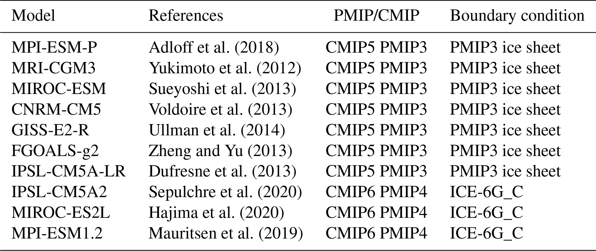
We forced GRISLI with the absolute climatic fields from general circulation model (GCM) outputs of the PMIP3/PMIP4 database (Kageyama et al., 2021). All the GCMs for which LGM simulations were available at the time of writing the article have been selected (see Table 1).

Table 1 PMIP3 and PMIP4 models used to force GRISLI. The fourth column indicates the choice of the ice sheet boundary condition at the LGM for each GCM simulation. Ice sheet reconstructions are used as a boundary condition of the GCM simulations at the LGM.

Monthly surface air temperatures and solid monthly precipitation are used to compute the surface mass balance defined as the difference between snow/ice accumulation and ablation. Ablation is calculated using a positive degree day (PDD) method, following the formulation of Tarasov and Peltier (2002), where the degree day factors, C_ice and C_snow, depend on the mean July surface air temperature. Snow accumulation is calculated from the total precipitation (rain and snow), considering only months where monthly temperatures are under the melting point.

Due to the differences between GCM and GRISLI resolutions, the GCM outputs are bi-linearly interpolated onto the ice sheet model grid. In addition, to account for orography differences between GRISLI and the GCMs, the surface air temperatures of the GCMs are corrected using a constant vertical temperature gradient λ=7 ^∘C km⁻¹,

$$\begin{array}{}\text{(4)}& T(t{)}_{\mathrm{GRISLI}}=T_{\mathrm{GCM}}^{\mathrm{LGM}}-\mathit{\lambda }\left(S\left(t\right)-S_{\mathrm{GCM}}^{\mathrm{LGM}}\right),\end{array}$$

where T(t)_GRISLI is the time-dependent surface air temperature at the surface elevation S(t) simulated by the ice sheet model, and $T_{\mathrm{GCM}}^{\mathrm{LGM}}$ and $S_{\mathrm{GCM}}^{\mathrm{LGM}}$ are the LGM surface air temperature and orography computed by the GCMs. This temperature correction induces a change in precipitation, which is computed following the Clausius–Clapeyron formulation for an ideal gas:

$$\begin{array}{}\text{(5)}& \mathrm{pr}(t{)}_{\mathrm{GRISLI}}={\mathrm{pr}}_{\mathrm{GCM}}^{\mathrm{LGM}}\cdot \exp \left(\mathit{\omega }\cdot \left(T(t{)}_{\mathrm{GRISLI}}-T_{\mathrm{GCM}}^{\mathrm{LGM}}\right)\right),\end{array}$$

where pr(t)_GRISLI is the precipitation calculated by GRISLI at each time step, and ${\mathrm{pr}}_{\mathrm{GCM}}^{\mathrm{LGM}}$ is the LGM precipitation computed by the GCM and interpolated on the GRISLI grid. ω is the precipitation ratio to temperature change and is fixed to 0.11 ^∘C⁻¹ (Quiquet et al., 2013).

Following Pollard and DeConto (2012), the sub-shelf melt rate (OM) is computed using ocean temperature and salinity:

$$\begin{array}{}\text{(6)}& \mathrm{OM}=K_{\mathrm{t}}{\displaystyle \frac{{\mathit{\rho }}_{\mathrm{w}}{C}_{\mathrm{w}}}{{\mathit{\rho }}_{\mathrm{i}}{L}_{\mathrm{f}}}}\left|T_{\mathrm{o}}-T_{\mathrm{f}}\right|\left(T_{\mathrm{o}}-T_{\mathrm{f}}\right),\end{array}$$

where K_t is called the transfer factor and is set to 7 m yr^−1 ∘C⁻¹ in the baseline experiments, as in Pollard and DeConto (2012). ρ_w is the ocean water density, ρ_i is the ice density, L_f is the latent heat of ice fusion, C_w is the specific heat of ocean water, and T_o is the local ocean temperature. T_f is the local freezing point temperature, depending on the ocean salinity (S), and is computed using the Beckmann and Goosse (2003) parameterization:

$$\begin{array}{}\text{(7)}& T_{\mathrm{f}}=\mathrm{0.0939}{}^{\circ }\mathrm{C}-S\times \mathrm{0.057}{}^{\circ }\mathrm{C}+z\times \mathrm{7.64}\times {\mathrm{10}}^{-\mathrm{4}}{}^{\circ }\mathrm{C},\end{array}$$

where z is the ocean depth.

Table 2 Model parameters of the GRISLI ice sheet model used in this study.

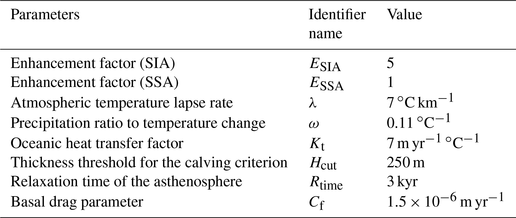
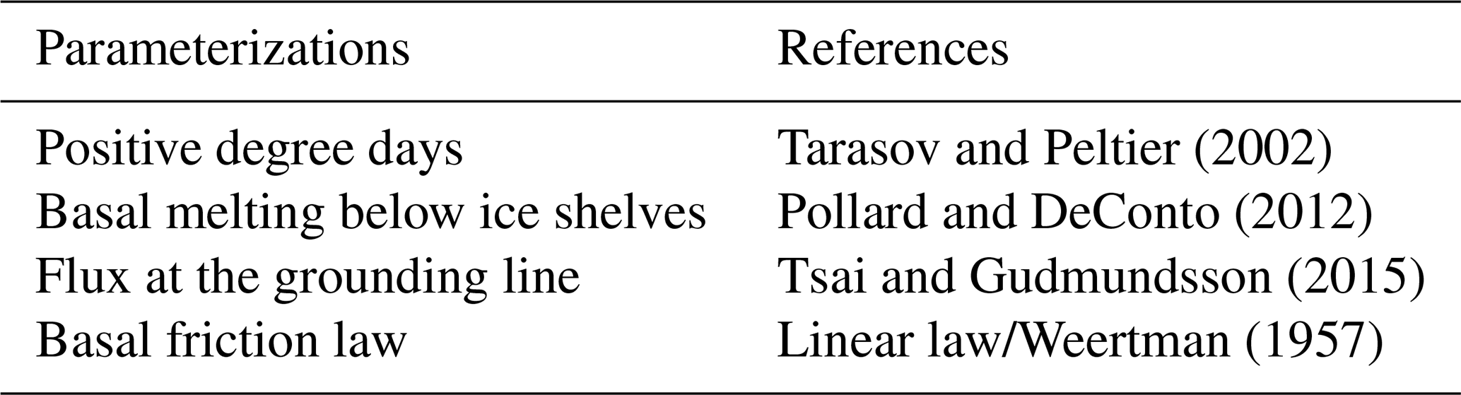
Table 3 Parameterizations of the GRISLI ice sheet model used in this study.

A difficulty related to the oceanic forcing fields is that the GCMs do not provide any oceanic information outside their land–sea mask and under the ice shelves. To fill these gaps, we performed a classical near-neighbour horizontal extrapolation of temperature and salinity, except that we perform this extrapolation within 10 sectors independently. These sectors roughly correspond to drainage basins (Fig. S1 in the Supplement). The definition of these basins is based on bedrock topographic features and LGM ice elevation and is somehow comparable to the approach followed by Zwally et al. (2015) for Antarctica. The horizontal extrapolation is performed for each individual vertical layer, without any vertical interpolation. This extrapolation method provides information on temperature and salinity within the entire ice shelf cavity for each vertical level of the GCMs. These temperature and salinity fields are then used to compute the sub-shelf melt rate (Eq. 6), using a linear vertical interpolation between the two oceanic layers bounding the ice shelf depth. The only exception is when the PMIP3/PMIP4 simulations do not provide data in a given sector. In this case, a constant and homogeneous basal melting value of 0.1 m yr⁻¹ is prescribed. This mainly occurs in the continental southern flanks of the Eurasian ice sheet.

In GRISLI, each grid point can either be a floating or a grounded ice point. To account for the fact that the sub-shelf melt rate is higher in the vicinity of the grounded line (Beckmann and Goose, 2003), and due to the coarse resolution of the model, we apply a fraction of the neighbouring floating sub-shelf melt rate to the last grounded point, as in Pollard and DeConto (2012). This approach allows us to take the potential influence of the ocean into account.

The main parameters and parameterizations used in this study are shown in Tables 2 and 3.

2.3 LGM equilibrium

As mentioned above, the main objective of the present paper is to investigate the mechanisms responsible for the EIS retreat from its LGM configuration. To do this, a preliminary step is to build the EIS at the LGM.

We performed 100 kyr spin-up experiments (one for each GCM) forced by a constant LGM climate provided by the 10 GCMs. Simulations start with no ice sheet, and the eustatic sea level is prescribed at 120 m below the present level. The initial bedrock topography corresponds to the present-day topography from ETOPO1 (Amante, 2009). This procedure is required to obtain internal ice sheet conditions in equilibrium with the climate forcing and to examine whether the LGM climate can build and maintain the EIS when it is used as input to the GRISLI ice sheet model. From this climate forcing ensemble, we only selected those leading to LGM ice sheets in a reasonable agreement with the most credible ice extent in the DATED-1 database (Hughes et al., 2016) and with the geologically constrained ice thickness reconstructions, namely ICE-6G_C (Peltier et al., 2015), GLAC-1D (Briggs et al., 2014; Tarasov et al., 2012; Tarasov and Peltier, 2002), and ANU (Lambeck, 1995, 1996; Lambeck et al., 2010).

2.4 Sensitivity experiments

To quantify the relative importance of the three main drivers (i.e. surface mass balance, sub-shelf melt rate, and sea level) of the EIS retreat, we applied time-constant perturbations on the atmospheric and oceanic GCM forcings, and we changed the prescribed sea level. The perturbed simulations are run for 10 kyr. We analysed the response at year 1000 of the simulation to investigate the impacts of climate changes that may have occurred at the beginning of the deglaciation and at year 10 000 to examine the sensitivity of EIS on longer timescales.

In the first series of experiments (EXP1), we investigate the effect of SMB changes by increasing surface air temperatures. During the last deglaciation (21–8 ka), the mean annual global surface air temperature increased by $\mathrm{4.5}{}^{\circ }\pm \mathrm{0.9}{}^{\circ }$ (Annan et al., 2022). In order to simulate a range of anomalies representative of the onset of the last deglaciation, we chose to apply perturbations from 1 to 5  ^∘C to the mean annual GCM forcing fields, without accounting for related changes in precipitation (see Eq. 5).

We know from the Clausius–Clapeyron relationship that the water content in the atmosphere is directly related to atmospheric temperature. An increase in atmospheric temperature can therefore lead to an increase in precipitation. This is what is currently being observed in eastern Antarctica (Frieler et al., 2015). As a result, the increase in precipitation in response to increased temperatures (Eq. 5) is considered in the second set of experiments (EXP2).

The third series of experiments (EXP3) is designed to assess the role of oceanic forcing on the EIS stability. Because the basal melting below the ice shelves depends linearly on the K_t transfer coefficient and is a quadratic function of the oceanic temperatures, we performed two sub-series of experiments by modifying either the K_t values (EXP3.1) without modifying the oceanic temperatures or by applying perturbations to the oceanic temperatures (EXP3.2). Observations below the Antarctic ice shelves show that the basal melting rate ranges from 0 to 35 m yr⁻¹ for oceanic temperatures between −2 and 2 ^∘C (Holland et al., 2008). This wide range of basal melting rate values reflects the complexity of such a process that can only be partially represented with simple parameterizations (Eq. 6). The K_t coefficient is thus largely uncertain. Therefore, to investigate changes in the EIS sensitivity to the amplitude of basal melting, we first use a wide range of values for this transfer coefficient, i.e. between 10 and 50 m yr^−1 ∘C⁻¹.

The mean global sea surface temperature anomaly inferred from the MARGO project (MARGO project members, 2009) between the Late Holocene and the LGM is 1.9±1.8 ^∘C consistent with the findings (∼2.7 ^∘C) of Tierney et al. (2020). In the early phase of the deglaciation, the ocean warming was probably less than that of the Late Holocene. Therefore, for the EXP3.2 experiments, we first apply perturbations of 0.5, 1.0, and 1.5 ^∘C to the oceanic temperatures (same perturbation on all vertical levels), and we fix the K_t coefficient to 7 m ^∘C⁻¹ yr⁻¹. In the transient simulation of the last deglaciation performed by Liu et al. (2009), large increases in oceanic temperatures are obtained. For example, a +9 ^∘C warming is obtained in the Bjørnøyrenna (BJR) sector at 500–600 m ocean depth and almost 7.5 ^∘C in the Svyataya Anna (SA) sector at 400–500 m. To reproduce the large increase in the subsurface ocean temperature obtained in Liu et al. (2009), we performed additional sensitivity experiments with perturbations of 7.5 and 10 ^∘C applied in the entire oceanic column.

Atmospheric and oceanic temperatures are the two main factors potentially responsible for the destabilization of marine ice sheets. Thus, the fourth series of experiments (EXP4) combines surface air temperature perturbations ($\mathrm{\Delta }T=+\mathrm{2}$, +3, and +4 ^∘C) with basal melting rate perturbations (K_t=10, 15, and 25 m yr^−1 ∘C⁻¹).

In the fifth set of experiments (EXP5), we also explore the EIS sensitivity to sea level. Indeed, sea level rise favours the retreat of the grounding line and is therefore another potential driver of the marine ice sheet instability. At the beginning of the deglaciation, the global sea level increased by more than 10 m (Carlson and Clark, 2012), raising the global sea level from −120 to −110 m compared to the present-day eustatic sea level. This abrupt change may have played an important role in the destabilization of the ice sheet. On the other hand, Gowan et al. (2021) show that the local sea level around the EIS margin displays a significant spread at the LGM, from −70 to −140 m, compared to the present-day level and can abruptly change in response to variations in the land–ice mass distribution. Consequently, to better explore the EIS sensitivity to both global mean sea level and local sea level at the beginning of the last deglaciation, we apply moderate (−115, −110, and −105 m) and large (−90, −60, −30, and 0 m) sea level perturbations with respect to the present day.

3 Available ice sheet reconstructions and ice stream signature

3.1 Ice sheet geometry

The DATED-1 database is based on evidence found in the existing literature and retrieved from various geological materials (e.g. terrestrial plant macrofossils, foraminifera, speleothems, and bones) analysed with a range of dating methods. Based on these data, the DATED-1 compilation provides three different scenarios for the maximal, minimal, and most credible EIS extent. The GLAC-1D, ICE-6G_C, and ANU reconstructions are based on inverse modelling approaches constrained by GPS data, relative sea level, and geomorphological data.

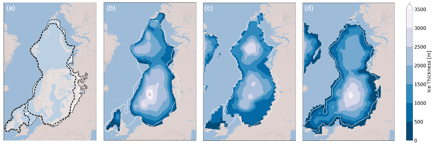
Figure 2 (a) Ice sheet extent at the LGM derived from the DATED-1 compilation (Hughes et al., 2016). The maximum and the minimum scenarios of the ice extent are represented by the dotted and the dashed lines, respectively. (b) Ice thickness at the LGM provided by the ANU reconstruction (Lambeck et al., 1995, 1996; Lambeck et al., 2010; Abe-Ouchi et al., 2015). Panel (c) is the same as panel (b) for the ICE-6G_C reconstruction (Peltier et al., 2015). Panel (d) is the same as panel (b) for the GLAC-1D reconstruction (Briggs et al., 2014; Tarasov et al., 2012; Tarasov and Peltier, 2002). In each of the four panels, the white line corresponds to the most credible scenario of the ice extent at the LGM derived from the DATED-1 compilation (Hughes et al., 2016).

The main differences in the three DATED-1 scenarios at the LGM (Hughes et al., 2016) are related to the potential BIIS–FIS connection (or disconnection), which is the southern continental limit of the FIS and the eastern limit of BKIS (Fig. 2a). Only the minimum scenario suggests the absence of ice between the BIIS and FIS.

The GLAC-1D reconstruction agrees well with the most credible DATED-1 scenario, despite a slightly greater ice extent in most of the Fennoscandian regions and a smaller extent in the Taymyr Peninsula (in the easternmost part of the BKIS; Fig. 2d). This contrasts with the ANU and ICE-6G_C reconstructions whose ice limit goes beyond that of the most credible DATED-1 scenario.

The differences between the three geologically constrained reconstructions are due to differences in the inverse methods used to estimate the ice thickness, the geological and geomorphological data considered to infer the ice extent, and the different choices regarding the Earth rheology. This translates into differences in the altitude of the EIS. For example, in the ANU and GLAC-1D reconstructions, the FIS peaks at 3000–3500 m, while BKIS does not exceed 2500 m (2000 m for GLAC-1D). In contrast, ICE-6G_C provides a larger ice thickness over the BKIS sector (2500–3000 m) than over Fennoscandia.

3.2 Ice stream signature

Ice streams also play a key role in ice sheet dynamics and in featuring ice sheet geometry (Pritchard et al., 2009). It is therefore crucial that the dynamics of the simulated ice sheets is consistent with reconstructions. The signature of ice streams can be inferred from geomorphological observations in the Barents Sea, in particular those of the Bjørnøyrenna (BJR) and Svyataya Anna (SA) ice streams (Fig. 1) (Polyak et al., 1997; Andreassen and Winsborrow, 2009; Dowdeswell et al., 2016, 2021; Szuman et al., 2021). Other geomorphological observations strongly suggest the existence of palaeo ice streams in the FIS, such as the mid-Norwegian (MN) ice stream (Stokes and Clark, 2001), and the Norwegian Channel (NC) ice stream between the FIS and BIIS (Sejrup et al., 1994; Svendsen et al., 2015; Stokes, 2001).

4 Results

4.1 LGM equilibrium

At the end of the 100 kyr spin-up simulations, a wide range of ice sheet geometries is obtained (Fig. 3). In the same way as Niu et al. (2019), we show that simulations performed with CNRM-CM5 and MRI-CGM3 do not succeed in maintaining ice cover over Eurasia to the same extent as in the reconstructions. In addition, we show that the simulation forced by MIROC-ES2L also fails to form an ice sheet.

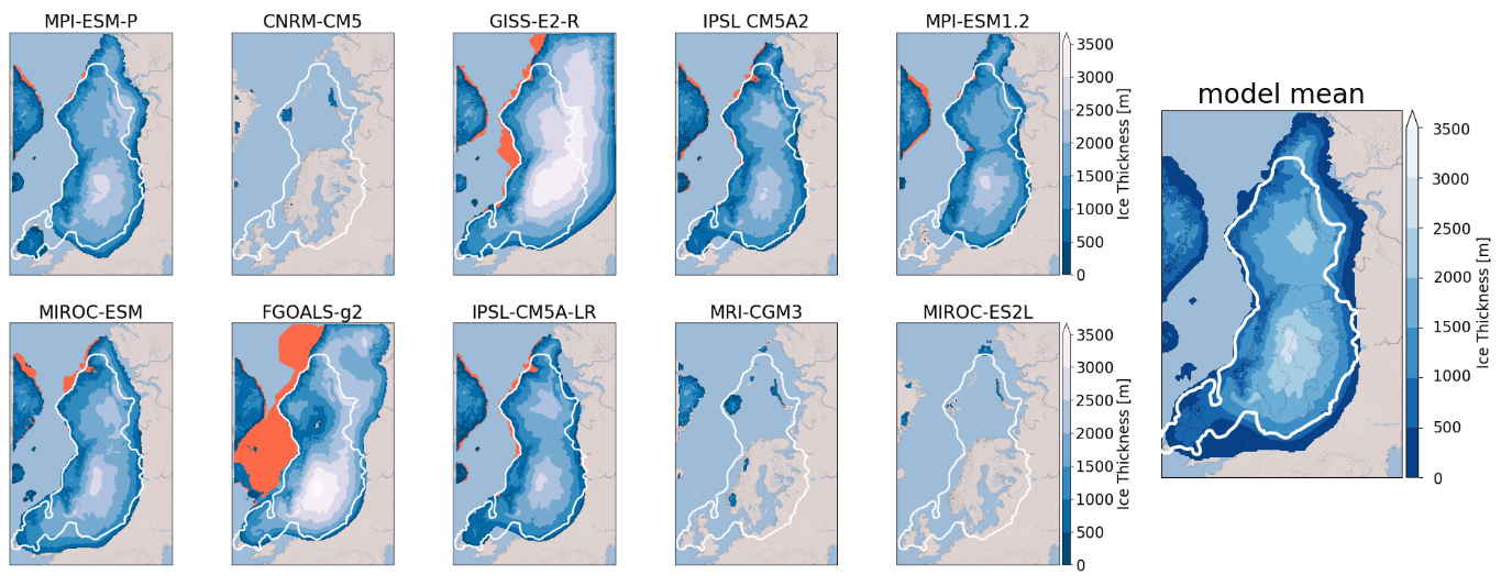
Figure 3 Ice thickness at the end of the 100 kyr simulation for the different GCMs used as the forcing of the GRISLI ice sheet model. The white line is the most credible extent derived from the DATED-1 compilation, and the orange shaded areas are the simulated ice shelves. The multi-model mean of the five selected ice sheets is shown in the right panel.

This is primarily explained by high positive summer surface air temperatures simulated by the three models in most parts of the EIS compared to the other models, with temperature anomalies ranging between +4.7 and +11.7 ^∘C (Fig. 4). Conversely, with the GISS-E2-R and FGOALS-g2 models, significant ice thickness is built east and south of BKIS because of strong negative mean summer temperatures in this area (Fig. 4).

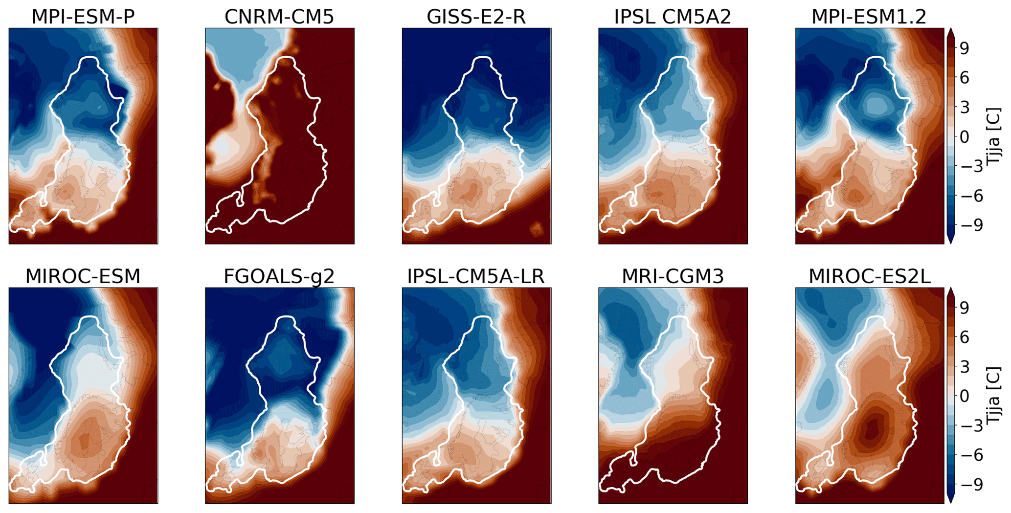
Figure 4 Mean summer (JJA) surface air temperature at 21 ka simulated by each GCM at the sea level and interpolated on the GRISLI grid. The white line represents the ice extent, as defined by the most credible DATED-1 scenario.

Therefore, we discarded these models and only selected those (MPI-ESM-P, MIROC-ESM, IPSL-CM5A2, IPSL-CM5-LR, and MPI-ESM1.2) providing ice sheet geometries in relatively good agreement with the reconstructions.

The five selected ice sheets do not show significant differences (Fig. 3). The FIS peaks at 2500–3000 m, while the BKIS is lower (2000–2500 m), due to a drier atmosphere compared to that overlying the Fennoscandian region (Fig. 5). The simulated FIS agrees with the ICE-6G_C reconstruction, despite a flatter dome simulated with MPI-ESM-P, which is about 500 m lower compared to GLAC-1D and ANU. Conversely, the BKIS maximum altitude simulated by GRISLI is underestimated compared to ICE-6G_C, while it is in good agreement with the two other reconstructions. The BKIS margins bordering the Greenland and Norwegian seas and the Arctic Ocean generally match with the most credible DATED-1 scenario of the ice extent. However, in the five GRISLI simulations, the ice extent is too large in the eastern and southern edges compared to DATED-1.

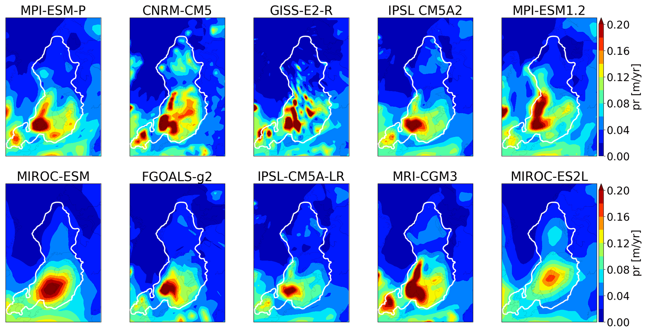
Figure 5 Same as Fig. 4 for the mean annual precipitation.

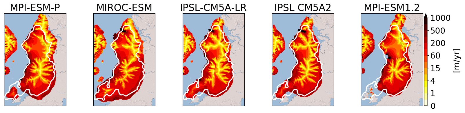
Figure 6 Simulated ice velocities at the end of the 100 kyr LGM simulation. The solid white line represents the most credible ice extent from the DATED-1 compilation.

The most likely cause of this mismatch is related to the imprint of the ice sheet reconstructions used as boundary conditions of GCM simulations. Indeed, both the ice sheet reconstruction used for PMIP3 simulations (not shown) and ICE-6G_C (Fig. 2c) used in PMIP4 runs overestimate the ice extent in the region of the Taymyr Peninsula. This results in an enhanced cooling favouring the simulated ice expansion in this area. This effect can be amplified by the projections of the ice sheet reconstructions on the coarser GCM grid that may produce an artificial spread of the ice sheet mask, further causing a cooling that is too extended. Another source of disagreement between DATED-1 and the simulated ice sheets can be due to the representation of the jet stream and planetary waves in the coarse-resolution climate models, such as the PMIP models. Indeed, such large-scale atmospheric features directly impact the simulated precipitation and temperatures and may cause too much precipitation or too much cooling if improperly represented (Liakka and Lofverstrom, 2018).

For the five selected GCMs, areas with high ice velocities are simulated in the BKIS region (Fig. 6). The highest velocities are obtained for the SA, BJR, NC, and MN ice streams and can exceed 1000 m yr⁻¹. In addition, the BJR ice stream shows a large extension from the centre of BKIS, with velocities between 75 and 200 m yr⁻¹, to the edge of BKIS. The location of the main fast-flowing areas is consistent with empirical evidence, based on observations of submarine landforms (Dowdeswell et al., 2016; Stokes, 2001). It is also interesting to mention that ice velocities of similar magnitude in the present-day Antarctic and Greenland ice sheets have been revealed, thanks to radar observations (Solgaard et al., 2021; Mouginot et al., 2019).

Overall, our five remaining simulated ice sheets show a reasonable agreement with the different reconstructions constrained by geological and geomorphological observations, both in terms of ice extent and ice thickness, as well as dynamical characteristics. The observed differences with the reconstructions remain within the range of uncertainties, which is itself illustrated by the differences between the three reconstructions GLAC-1D, ANU, and ICE-6G_C and by the three ice extent scenarios from the DATED-1 compilation.

This allows us to use the five spin-up GRISLI experiments (forced by MPI-ESM-P, MIROC-ESM, IPSL-CM5A2, IPSL-CM5-LR, and MPI-ESM1.2) as a starting point to test the sensitivity of the EIS to atmospheric, oceanic, and sea level forcings.

4.2 Sensitivity experiments

In the following, we investigate the sensitivity of the Eurasian ice sheet to the potential drivers of ice sheet retreat: atmospheric changes responsible for SMB changes (i.e. temperature and snow accumulation to the first order); oceanic changes (sub-shelf melt rate); and sea level changes.

4.2.1 EXP1: surface air temperature

The aim of this section is to investigate the sensitivity of EIS to a temperature rise. For each temperature perturbation (T_add=1 to 5 ^∘C) applied uniformly on the monthly mean surface air temperatures, Fig. 7 displays for the multi-model mean the percentage of the ice thickness lost after 1 kyr with respect to the initial configuration. The results are plotted for the largest ice sheet mask. This mask corresponds to all areas where ice has been simulated in at least one of the five simulations. This means that multi-model means are computed with one, two, three, four, or five models involved, depending on the ice sheet mask of each individual model.

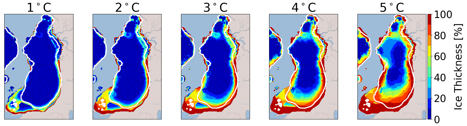
Figure 7 Multi-model mean of the ice thickness lost after 1 kyr of the GRISLI model in the EXP1 experiments with respect to the ice thickness of the LGM ice sheet (red means 100 % lost). The results are plotted on the largest ice sheet mask. The white line corresponds to the common ice sheet mask of the five models (i.e. where the multi-model mean is computed on the five models).

For T_add=1 ^∘C, the response of the Eurasian ice sheets is weak, except for the British Isles sector (Fig. 7) for which mean June to August (JJA) temperatures of the five selected GCMs are close to the melting point (Fig. 4). Substantial ice losses are also simulated in the FIS margins for temperature rises greater than 1 ^∘C, leading to a progressive retreat of the edge of the ice sheet as the temperature increases. The sensitivity of the BIIS and FIS regions to these temperature perturbations is explained by a shift from positive to negative SMB values when temperature increases (Fig. S2). In contrast, as the BKIS is located in colder areas, larger temperature perturbations (3 to 5 ^∘C) are necessary to initiate the ice sheet's retreat. The southern BKIS margin appears as the most sensitive region, followed by the region of the SA ice stream. In the SA sector, ice thickness losses between 30 % ($T_{\mathrm{add}}=+\mathrm{3}$ ^∘C) and 50 % ($T_{\mathrm{add}}=+\mathrm{5}$ ^∘C) are obtained. In the BJR sector, ice losses are only simulated for large temperature perturbations.

However, it is worth mentioning that for a given temperature perturbation, significant differences in the behaviour of the five simulated ice sheets can be observed. To illustrate these differences, we plotted for each simulation the percentage of ice thickness lost after 1 kyr with respect to the initial configuration (Fig. S3). The most sensitive regions to surface air temperature, namely the FIS margins and the SA/BJR sectors, are the locations where inter-model differences in ice thickness losses are the most significant and are amplified with temperature increase. In the BJR sector, the retreat of the ice sheet is simulated for perturbations of 4 ^∘C with three GCM forcings (MIROC-ESM, IPSL-CM5A-LR, and IPSL-CM5A2; Fig. S3), while this sector is stable with the two other forcings (MPI-ESM-P and MPI-ESM1.2) under this temperature perturbation. In the SA sector, the MIROC-ESM-P forcing produces a retreat from a temperature anomaly of 2 ^∘C, but for the IPSL-CM5A-LR and IPSL-CM5A2 forcings, the retreat is only triggered for T_add=3 ^∘C. In contrast, the two versions of the MPI-ESM produce a more stable ice sheet in the SA sector since, even with a 5 ^∘C temperature perturbation, the ice retreat is not triggered within the 1 kyr of simulation.

The lower sensitivity of BJR sector, compared to the SA sector, can be explained (at least partly) by the topography differences between these two regions. Actually, the initial topography of each GCM (not shown) exhibits a trough in the SA sector which does not appear in the region of the BJR ice stream. The lower surface topography in the SA sector is accompanied by higher surface temperatures and thus to larger ice losses when temperature perturbations are applied (Fig. S3). Moreover, the difference in the sensitivity of the BJR and SA sectors can be also explained by the higher precipitation rate in the BJR sector (between 0.2 and 0.5 m yr⁻¹ for the BJR ice stream and less than 0.2 m yr⁻¹ for the SA sector; Fig. 5), which can partly counteract the effect of temperature increase on ice mass loss.

To better understand the effect of precipitation on the EIS stability, the EXP2 combines the precipitation and surface air temperature perturbations. The results obtained in the EXP2 experiments are shown in Fig. S4. For BIIS and FIS, a similar behaviour to EXP1 is observed, albeit with less ice melt, due to increased accumulation as a result of increased temperatures. On the contrary, in EXP2, a large difference with EXP1 is simulated for BKIS, where only the ice sheet margins show sensitivity to increased temperature and precipitation. While an inland ice loss between 20 % and 50 % was simulated in EXP1 in some places, it is generally limited to less than 10 % in EXP2. This result shows the significant role of precipitation to counteract the ice loss due to an increase in surface air temperature.

4.2.2 EXP3: basal melting

Besides changes in SMB, another factor that can destabilize a marine ice sheet is the basal melting under the ice shelves (Pritchard et al., 2012). In the LGM experiments, the numerical K_t value is fixed to 7 m ^∘C⁻¹ yr⁻¹ and leads to basal melting rates in the BJR and SA sectors of 3.1 and 0.7 m yr⁻¹, respectively. To investigate the effect of increased basal melting that likely occurred during the last deglaciation as a response to increased ocean temperatures, we performed sensitivity experiments by first changing the K_t value (EXP3.1). The sensitivity to oceanic temperatures (EXP3.2) will be discussed later.

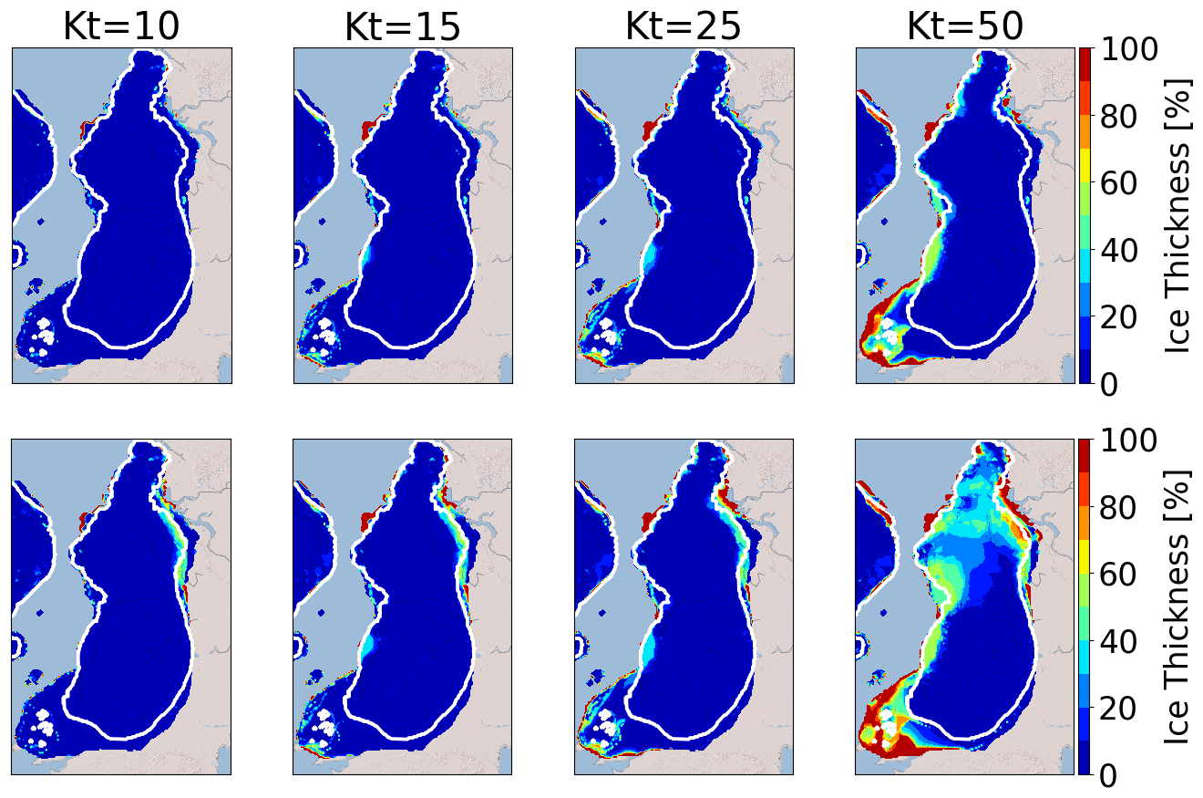
Figure 8 Multi-model mean of the ice thickness lost after 1 kyr (top panels) and 10 kyr (bottom panels) in the GRISLI model in the EXP3.1 experiments with respect to the ice thickness of the LGM ice sheet (red means 100 % lost). The white line corresponds to the common ice sheet mask of the five models (i.e. where the multi-model mean is computed on the five models). K_t is the transfer factor in Eq. (6) (expressed in m yr^−1 ∘C⁻¹).

Figure 8 displays the percentage of ice thickness losses (with respect to the initial configuration) for K_t ranging from 10 to 50 m ^∘C⁻¹ yr⁻¹. After 1 kyr of simulation, no change in ice thickness is observed for K_t=10 m ^∘C⁻¹ yr⁻¹. For higher K_t values (15 and 25 m ^∘C⁻¹ yr⁻¹), ice losses between 30 % and 40 % are simulated in the MN ice stream sector, and 100 % of the ice shelf in the south of SA sector is melted (see Fig. 3 showing the presence of ice shelves at the end of the spin-up experiment). This corresponds to basal melting rates (multi-model mean) near the grounding line ranging from 7.5 m yr⁻¹ (K_t=15 m ^∘C⁻¹ yr⁻¹) to 10.4 m yr⁻¹ (K_t=25 m ^∘C⁻¹ yr⁻¹) in the MN sector and from 1.7 m yr⁻¹ (K_t=15 m ^∘C⁻¹ yr⁻¹) to 2.9 m yr⁻¹ (K_t=25 m ^∘C⁻¹ yr⁻¹) in the SA sector. However, these changes are restricted to small areas, and the ice loss is not significant enough to firmly indicate a noticeable sensitivity to basal melting. Perturbations with K_t values above 25 m ^∘C⁻¹ yr⁻¹ are necessary to observe significant changes in the EIS configuration. In particular, for K_t=50 m ^∘C⁻¹ yr⁻¹, the ice is entirely melted near the BIIS margins, and less than 50 % of the ice remains in the regions of the MN, SA, and BJR ice streams. Nonetheless, only the simulations forced by MPI-ESM-P, MPI-ESM1.2, and MIROC-ESM show a sensitivity to basal melting in the BJR, MN, and SA sectors (Fig. S5). Depending on the GCM forcing, the simulated basal melting values range between 25.7 and 28.7 m yr⁻¹, 24.4 and 28.2 m yr⁻¹, and 11.2 and 13.4 m yr⁻¹ for the BJR, MN, and SA sectors, respectively. In contrast, very small values are obtained with IPSL-CM5A2 (0.2–0.5 m yr⁻¹) and IPSL-CM5A-LR models (0.5 m yr⁻¹). This can be explained by the cold oceanic temperatures near the BJR sector compared to those simulated by the three other GCMs (Fig. S6). These results show that the basal melting has the ability to destabilize the BKIS when it exceeds a certain threshold. Results inferred from the simulations forced by MPI-ESM-P, MPI-ESM1.2, and MIROC-ESM suggest that this threshold is obtained for K_t values between 25 and 50 m ^∘C⁻¹ yr⁻¹, corresponding to basal melting rates at the grounding line between 10.4 and 28.7 m yr⁻¹ for the BJR sector and between 6.2 and 13.4 m yr⁻¹ for the SA sector. By comparison, a basal melting rate of 22 m yr⁻¹ has been observed, thanks to radar measurements in the mouth of the Mercer–Whillans ice streams located in the West Antarctic ice sheet (Marsh et al., 2016). Providing that K_t values are greater than 25 m ^∘C⁻¹ yr⁻¹ (or close to 50 m ^∘C⁻¹ yr⁻¹), the region of the BJR ice stream responds to basal melting perturbations with basal melting rates similar to those observed in some parts of the WAIS. However, the ice loss is restricted to the very edge of the ice sheet, and the BKIS retreat is negligible. This raises the question as to whether the basal melting exerts a stronger influence on longer timescales. Therefore, we also investigated the ice sheet behaviour after 10 000 model years.

A similar behaviour is observed after 10 kyr for K_t between 10 and 25 m ^∘C⁻¹ yr⁻¹, with the exception of the southern part of BKIS bordering the Kara Sea, where a 30 % to 50 % ice thickness decrease, with respect to the initial one, is obtained. For K_t=50 m ^∘C⁻¹ yr⁻¹, more than 40 % of the ice loss is simulated for BKIS and up to 60 % in the BJR sector. As previously mentioned, this large ice thickness decrease in the centre of BKIS is highly GCM dependent and is only observed in simulations forced by the MIROC and MPI models (Fig. S5).

As the basal melting parameterization is expressed as a quadratic function of the oceanic temperatures, we may expect a different sensitivity of EIS when the oceanic temperatures increase (EXP3.2). Results of the EXP3.2 experiments are shown in Fig. S7. Perturbations of oceanic temperatures between +0.5 and +1.5 ^∘C lead to basal melting rates at the grounding line of the BJR sector of less than 3.8 m yr⁻¹. This is well below the threshold suggested by the results of the EXP3.1 experiments (between 10.4 and 30 m yr⁻¹), and no significant ice loss is simulated after 10 kyr of simulation.

For larger perturbations (+7.5 and +10 ^∘C), larger values of the basal melting rates are obtained in the BJR (11.6 and 17.5 m yr⁻¹), in the SA (10.8 and 15.6 m yr⁻¹) and in the MN sectors (11.5 and 17.4 m yr⁻¹) after 10 000 model years. A perturbation of 7.5 ^∘C does not trigger the ice retreat because of basal melting that is too low. In contrast, when the perturbation reaches +10 ^∘C, a similar behaviour to that simulated with K_t=50 m ^∘ C⁻¹ yr⁻¹ (EXP3.1) is obtained.

On the other hand, for simulations forced by IPSL-CM5A2 and IPSL-CM5A-LR, an increase in oceanic temperatures of +10 ^∘C allows us to observe a sensitivity of BKIS in the SA sector (see Fig. S8) after 1 kyr of simulations, which leads to a total retreat of the eastern part of BKIS after 10 kyr.

These results show that the BJR, MN, and SA regions are sensitive to sub-shelf melting, providing that the basal melt exceeds a certain threshold obtained for K_t values greater than 25 m ^∘C⁻¹ yr⁻¹ (and greater than 10 m ^∘C⁻¹ yr⁻¹ for the MN sector) or for a rise in oceanic temperature greater than 7.5 ^∘C. From the combination of the EXP3.1 and EXP3.2 experiments, it appears that the threshold is between 11.6 and 17.5 m yr⁻¹ for the BJR sector, between 6.2 and 13.4 m yr⁻¹ for the SA sector, and lower than 7.5 m yr⁻¹ for the MN sector. Moreover, our results also suggest that the large retreat of one single ice stream has the ability to favour the total retreat of the whole of BKIS.

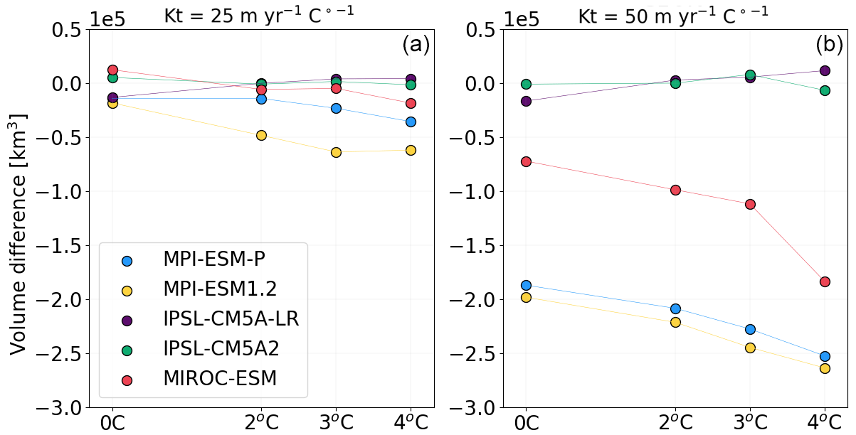
Figure 9 Differences in the ice volume lost between EXP4 and EXP1 (ΔV₄₋₁) after 1 kyr for K_t=25 m ^∘C⁻¹ yr⁻¹ (a) and K_t=50 m ^∘C⁻¹ yr⁻¹ (b).

4.2.3 EXP4: combined effects of basal melting and surface air temperatures

Results presented in the previous section suggest that sub-shelf melting has only a poor impact on the EIS destabilization for K_t perturbations below a certain threshold estimated to lie between 25 and 50 m ^∘C⁻¹ yr⁻¹ or below a +10 ^∘C increase in the oceanic temperatures. However, increases in surface melting due to atmospheric warming may lead to changes in the geometry of the grounded ice sheet and floating ice shelves. In turn, changes in the EIS configuration may alter the EIS sensitivity to basal melting. To test this hypothesis, we combined surface air temperature perturbations with basal melting perturbations (EXP4) and compared the results with those of the EXP1 experiments. Figure 9 displays the difference in the total BKIS ice volume after 1 kyr between the EXP4 and EXP1 experiments (ΔV₄₋₁) for different surface atmospheric temperature perturbations ($\mathrm{\Delta }T=+\mathrm{2}$, +3, and +4 ^∘C) and K_t values fixed to 25 and 50 m ^∘C⁻¹ yr⁻¹ (negatives values are associated with a greater ice loss in EXP4 than in EXP1). For both K_t perturbations (K_t=25 and 50 m ^∘C⁻¹ yr⁻¹), no significant difference in the ΔV_{4_1} values (computed for the different ΔT perturbations) is observed in simulations forced by IPSL-CM5A2 and IPSL-CM5A-LR. This illustrates the poor sensitivity of BKIS to basal melting with the IPSL climate forcings. As explained in Sect. 4.2.2, this low sensitivity is due to the cold oceanic temperatures simulated in both IPSL models (see Fig. S6). For the three other simulations (forced by MIROC-ESM, MPI-ESM-P, and MPI-ESM1.2), the ice volume difference is clearly amplified with higher ΔT levels, especially when the K_t transfer coefficient is higher. For example, for K_t=50 m ^∘C⁻¹ yr⁻¹, the difference in ΔV_{4_1} values between the initial ice sheet configuration (ΔT=0 ^∘C) and ΔT=4 ^∘C is ∼60 000 km³ with MPI-ESM-P, compared to ∼20 000 km³ when K_t=50 m ^∘C⁻¹ yr⁻1. Similar behaviour is observed for simulations forced by MIROC-ESM (∼110 000 km³) and MPI-ESM1.2 (∼60 000 km³). To better illustrate the impact of the combination of both temperature and basal melting perturbations, we plotted the evolution of ice loss every 1 kyr, as simulated in the EXP1 ($\mathrm{\Delta }T=+\mathrm{4}$ ^∘C), EXP3 (K_t=50 m ^∘C⁻¹ yr⁻¹), and EXP4 experiments in Figs. S9–S11. For the simulation forced by MIROC-ESM (Fig. S11), the largest part of the deglaciation signal is dominated by increased atmospheric temperatures in the EXP4 (see Fig. S11). Simulations forced by MPI-ESM-P and MPI-ESM1.2 have a different behaviour (Figs. S9 and S10) and show a significant difference between EXP1 and EXP4 and between EXP3 and EXP4. In the EXP3 experiment, the SA sector appears to be highly sensitive, mainly due to high ocean temperatures (>3 ^∘C; see Fig. S6), which is in contrast to the BJR sector, where only a part has deglaciated after 10 kyr. However, in the EXP4 experiment, in which near-surface temperature and basal melting are combined, BKIS starts to retreat after 1 kyr and has almost entirely melted after 10 kyr. This suggests that the BKIS deglaciation is initially triggered by surface warming but is further amplified by basal melting.

4.2.4 Exp5: sea level

In the previous simulations, the sea level forcing was fixed to −120 m (with respect to the present-day eustatic sea level), corresponding to the estimated eustatic level at the LGM (Peltier, 2002). In this series of experiments, we quantify the sensitivity of the EIS to different sea level forcings.

The multi-model mean difference between the ice thickness after 1000 GRISLI model years and the initial ice thickness (sea level = −120 m) is displayed in Fig. 10 for the different sea level elevations ranging from −115 to 0 m. After 1 kyr of simulation, for sea levels ranging from −115 to −105 m, no significant differences are observed with respect to the reference simulation (i.e. −120 m). For larger perturbations, the MN ice sheet sector appears to be the most sensitive. As an example, for a sea level of −90 m, an ice loss of ∼40 % is simulated in this area, and an almost complete retreat is obtained for a sea level higher than −60 m, with an ice thickness decrease of up to 80 %–100 %. Although sea level elevations of −90 and −60 m are considerably larger than the global mean sea level at the LGM, they are consistent with the local sea level variations that could be as high as −70 m, as suggested by Gowan et al. (2021). However, for the other sectors (BJR, SA, and NC ice sheet), the ice thickness decrease is only obtained for sea levels higher than −30 m, which is largely out of the range advanced by Gowan et al. (2021). As a result, this series of experiments conducted with the GRISLI model suggests that the elevation of sea level has only played a marginal role at the beginning of the EIS deglaciation.

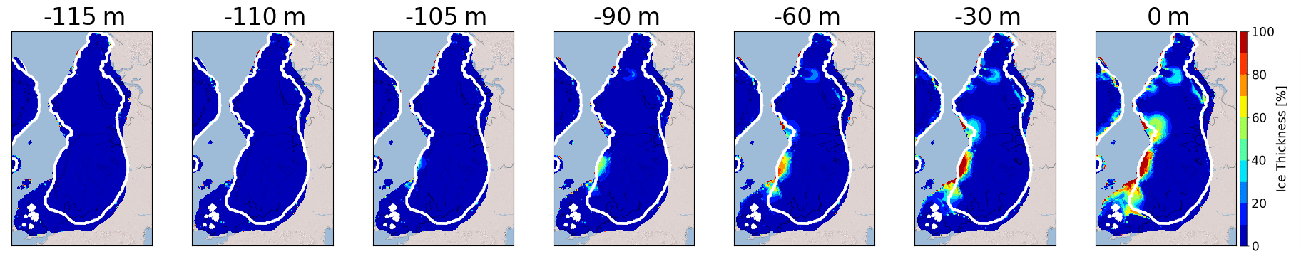
Figure 10 Multi-model mean of the ice thickness lost after 1000 model years in EXP5 with respect to the ice thickness of the LGM ice sheet (red means 100 % lost). The white line corresponds to the common ice sheet mask of the five models (i.e. where the multi-model mean is computed on the five models).

However, it should be noted that sea level rise can lead to changes in the geometry of the ice sheet and floating ice shelves. Therefore, these changes in the EIS configuration may influence its sensitivity to oceanic temperature perturbations. We tested this hypothesis by raising the sea level from −120 to −110 m compared to the current level and by concomitantly raising the oceanic temperatures (+1.5 and +10 ^∘C). Adding a sea level perturbation to the oceanic temperature perturbation does not drastically change the response of the ice sheet. Differences of 6 % to 7 % in ice volume losses were only observed for the highest temperature perturbation (+10 ^∘C) after 10 kyr for only two GCM forcings (MIROC-ESM and IPSL-CM5A2), while the differences are negligible (lower than 2 %) for smaller perturbations, shorter timescales and other GCM forcings (not shown).

4.3 Sensitivity to the spin-up method

The construction of spin-up is one of the most important factors impacting the sensitivity of the EIS. The LGM ice sheets presented in Sect. 4.1 were constructed under a constant LGM climate during 100 kyr. The specificity of this method is to construct ice sheets in good equilibrium with their environment. However, as outlined by Batchelor et al. (2019), the EIS was far from being in equilibrium with the climate at the LGM.

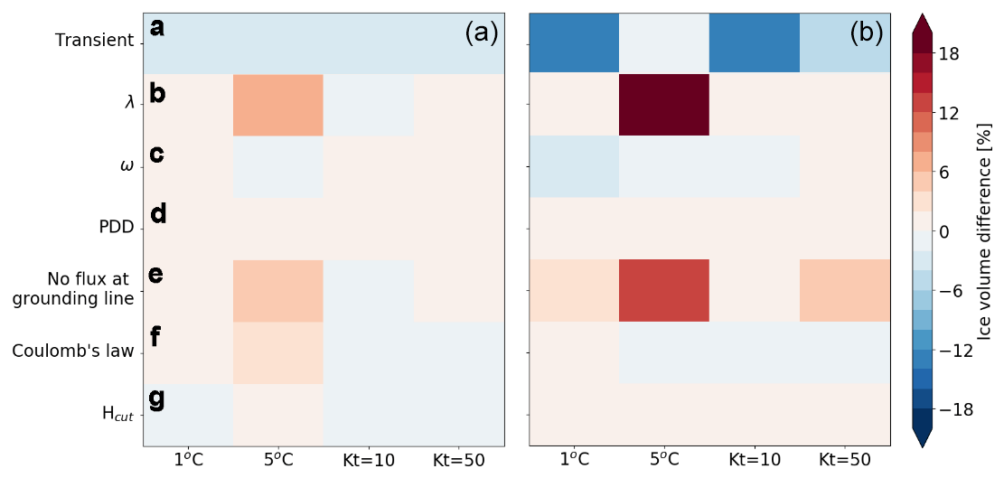
Figure 11 Multi-model mean of the differences in ice volume loss between the new perturbed simulations and the reference simulations (EXP1 and EXP3) after 1 kyr (a) and after 10 kyr (b). Note that the multi-model mean is done without the contribution of MIROC-ESM forcing for panel (a). The volume difference is calculated thanks to Eq. (8). λ is the vertical temperature gradient, ω is the ratio precipitation/temperature change, and H_cut is the calving criterion. More information is available in Table 4.

In order to look into the biases associated with the choice of the spin-up method, we compared the results obtained with a transient spin-up procedure. For this purpose, we reconstructed a climatology evolving from the Last Interglacial (−127 ka) to the LGM (−21 ka). The transition between these two climatic states is obtained by using a multi-proxy, following the same method as Quiquet et al. (2013). For the period between −127 and −122 ka, we used an index based on sea surface temperature (SST) reconstructions (McManus et al., 1999; Oppo et al., 2006), and from −122 to −21 ka, we chose an index based on North GRIP δ¹⁸O (North Greenland Ice Core Project members, 2004). In the same way as above, we used the 10 PMIP3/PMIP4 forcings shown in Table 1. As the Last Interglacial simulations were not available for some of the PMIP3/PMIP4 models, we made the approximation that the −127 ka climate was represented by the pre-industrial climate (i.e. piControl experiments; Eyring et al., 2016).

At the end of the of these new spin-up simulations, only four PMIP forcings (MPI-ESM-P, MPI-ESM1.2, IPSL-CM5A2, and IPSL-CM5A-LR) succeeded in constructing the EIS in agreement with the reconstructions (see Fig. S12h). Compared to previous LGM ice sheets presented in Sect. 4.1, the ice extent is smaller (Fig. S12h), and the dome of FIS is flatter with sharper edges. Furthermore, contrary to the previous method of spin-up construction (i.e. constant LGM forcing), the simulation forced by MIROC-ESM failed to form an ice sheet over the Barents Sea.

To assess the effect of the LGM EIS obtained after each of the transient spin-up experiment obtained with MPI-ESM-P, MPI-ESM1.2, IPSL-CM5A2, and IPSL-CM5A-LR, we applied atmospheric temperature perturbations (+1 and +5 ^∘C, as in EXP1) and basal melting perturbations (K_t values of 10 nd and 50 m ^∘C⁻¹ yr⁻¹, as in EXP3.1). Finally, we compare the percentage of remaining ice volume with the reference one (i.e. simulated in EXP1 and EXP3.1) and the new perturbed simulations after 1 and 10 kyr, using the following formula:

$$\begin{array}{}\text{(8)}& \begin{array}{rl}\mathit{\delta }& ={\displaystyle \frac{V_{\mathrm{pert}}(t=\mathrm{end})-V_{\mathrm{pert}}(t=\mathrm{0})}{V_{\mathrm{pert}}(t=\mathrm{0})}}\\ & -{\displaystyle \frac{V_{\mathrm{ref}}(t=\mathrm{end})-V_{\mathrm{ref}}(t=\mathrm{0})}{V_{\mathrm{ref}}(t=\mathrm{0})}}.\end{array}\end{array}$$

Each term on the right-hand side of Eq. (8) represents the percentage of ice volume loss in a given simulation. δ represents the difference (in %) in the ice volume loss between the new simulation and the reference simulation, with V_pert being the ice volume for the new perturbed simulation (transient spin-up) and V_ref the ice volume of the EXP1 and EXP3 simulations. A negative value of V_ice indicates a greater retreat of EIS of the new EIS configurations (i.e. obtained with the transient spin-up method).

Figure 11a shows the results of the computed δ value (see Eq. 8) after 1000 (left) and 10 000 model years (right) averaged over all models for atmospheric (1 and 5 ^∘C) and oceanic (K_t=10 and 50 m ^∘C⁻¹ yr⁻¹) perturbations. After 1 kyr, no significant difference is observed between both simulations. Conversely, after 10 kyr, a difference of the order of −10 % for perturbations of 1 ^∘C and 10 m ^∘C⁻¹ yr⁻¹ is observed. This can be explained by internal processes that are not in equilibrium with the LGM climate at the end of the transient spin-up simulation. More specifically, large differences in the simulated effective pressure are obtained at the end of both spin-up experiments. In the reference spin-up simulation (constant LGM climate), there is a relatively low effective pressure, since sub-glacial water has accumulated over the 100 kyr of the simulation (Fig. S13). In contrast, in the spin-up constructed by the transient method, large parts of the ice sheet are englacial for much shorter time periods, with smaller volumes of sub-glacial water resulting in higher effective pressure. This leads to drastically different sliding velocities among the two spin-up methods, with much smaller ice sheet velocities after the transient spin-up. During the perturbation experiments, the sub-glacial water tends to accumulate when using the transient spin-up ice sheet state. The temporal evolution in this case reflects the decrease in the effective pressure (and related increase in velocity) on top of the applied atmospheric or oceanic perturbation. The sensitivity over timescales greater than 1 kyr in these new experiments is thus not directly comparable to the reference sensitivity experiments in which the effective pressure is fully equilibrated.

4.4 Sensitivity to different GRISLI configurations

The results presented in Sect. 4.2 suggest that the EIS was primarily sensitive to atmospheric forcing at the beginning of the last deglaciation. However, we cannot exclude that this finding is specific to the choices of model parameters (Table 2) and physical parameterizations (Table 3). In order to assess the extent to which the observed EIS sensitivity is driven by these choices, we conducted additional experiments with alternative values of climate-related parameters (vertical temperature gradient, the precipitation ratio to temperature change, and degree day factors in the PDD formulation). We also changed the basal friction law and removed the parameterization of the ice flux at the grounding line (Table 4). We first performed 100 kyr simulations using the same procedure as for the reference simulations (Fig. S12a–g). Note that CNRM-CM5, GISS-E2-R, MIROC-ES2L, FGOALS-G2, and MRI-CGM3 fail to reproduce an ice sheet in agreement with the reconstructions, which is similar to our reference experiments (see Sect. 4.1 and 4.2).

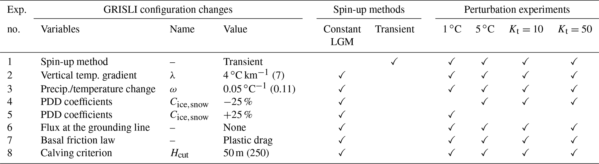
Table 4 List of sensitivity experiments (columns 5–10) performed with changes in the standard GRISLI configuration. New values of model parameters are given in column 4, with reference values indicated in parentheses. Changes in physical parameterizations are indicated in column 2.

Next, we applied atmospheric temperature perturbations (+1 and +5 ^∘C) and basal melting perturbations (K_t=10 and 50 m ^∘C⁻¹ yr⁻¹) to evaluate the relative importance of both atmospheric and oceanic forcings with the modified GRISLI configurations.

4.4.1 Sensitivity to climate parameters

First, we examined the sensitivity of EIS to a vertical temperature gradient of 4 ^∘C km⁻¹ (instead of 7 ^∘C km⁻¹), which is considered by Marshall et al. (2007) to be the most likely value of the near-surface temperature lapse rate. Therefore, a decrease in ice thickness of 100 m results in a decrease in atmospheric temperature of 0.4 ^∘C instead of 0.7 ^∘C (see Eq. 4). This choice aims at reducing the sensitivity of EIS to atmospheric forcing in order to analyse whether the ice sheet is more responsive to the oceanic forcing.

Second, in EXP2, we found that increased precipitation as a result of increased temperatures (see Eq. 5) tends to reduce the sensitivity of EIS. In the reference simulations (Sect. 4.2), the precipitation ratio to temperature change (ω value) was set to 0.11 ^∘C⁻¹. However, lower values can be found in the literature, ranging between 0.05 and 0.11 ^∘C⁻¹ (Petrini et al., 2020; Charbit et al., 2013; Quiquet et al., 2013). We therefore investigated whether the choice of a lower precipitation–temperature ratio, which is expected to lower the precipitation dependency to temperatures, could influence the response of the EIS. In this new series of sensitivity experiments, the ω parameter was fixed to 0.05 ^∘C⁻¹. In doing so, our objective is to assess whether a variation in ω can lead to significant changes in the response of the ice sheet to atmospheric forcing.

Last, Charbit et al. (2013) demonstrated that the choice of the PDD formulation can have a substantial impact on the computed amount of ice melt. In order to assess the impact on the stability of the EIS of the melt coefficient Cice and Csnow, as defined in Tarasov and Peltier (2002), we decreased (respectively, increased) their values by 25 % for the +5 ^∘C (+1 ^∘C) temperature perturbation. Decreasing (increasing) the melt coefficients by 25 % for the temperature perturbations allows us to reduce (increase) the influence of the atmospheric forcing on the evolution of the EIS. In addition, in order to reduce the influence of the surface air temperatures, we have also tested the impact of decreased melt coefficients in the basal melting perturbation experiments.

The results of these new sensitivity experiments are analysed in terms of differences in ice volume loss at 1 and 10 kyr with the reference simulations (δ value; see Eq. 8) and are displayed in Fig. 11b–d. The only significant differences with the reference simulations are obtained for a 5 ^∘C perturbation, due to a lowered temperature–elevation feedback in the simulation with λ=0.4 ^∘C km⁻¹. For all other experiments, changes in the ω parameter or in the degree day factors have differences of less than ±2 % compared to reference simulations. As such, this series of perturbed experiments shows that changing climate-related model parameters results in only small changes in the EIS ice volume loss compared to the standard configuration of the GRISLI ice sheet model and does not question the prevailing influence of the atmospheric forcing suggested by our reference sensitivity experiments.

4.4.2 Sensitivity to physical parameterizations

Besides the climate-related parameters, changes in the representation of the dynamic processes may have a strong impact on the relative importance of the mechanisms responsible for the triggering of the EIS retreat. For example, using the PSU ice sheet model (Pollard and DeConto, 2012), Petrini et al. (2018) found that the implementation of a grounding line flux adjustment reduces the sensitivity of BKIS. To go a step further and compare our findings with those of Petrini et al. (2018), we removed the grounding line flux parameterization in the GRISLI model and assessed its impact on the EIS sensitivity. Without the flux adjustment, the EIS sensitivity to basal melting and atmospheric temperature perturbations is reduced (Fig. 11e). This contrasts with the findings of Petrini et al. (2018). More specifically, after 10 kyr, a +5 ^∘C atmospheric perturbation results in a reduced amount of melting of about 14 % compared to the reference experiment (with parameterization of the grounding line flux). In other words, these results suggest that in the absence of the grounding line flux adjustment, higher atmospheric temperatures can potentially enhance the ice sheet's sensitivity to oceanic forcing through grounding line retreat.

Another source of huge uncertainties lies in the choice of the basal friction law (e.g. Brondex et al., 2017; Joughin et al., 2019; Åkesson et al., 2021). An appropriate choice of this law is of primary importance, as basal friction exerts a strong control on the dynamics of the grounding line and fast-flowing ice streams. In our previous experiments, the basal friction was parameterized using a linear dragging law (Eq. 2). In order to investigate the extent to which the choice of the friction law can influence the sensitivity of the EIS to atmospheric temperature and basal melting perturbations, we used a plastic dragging law, where the basal drag depends quadratically on the basal velocity (Pattyn, 2017).

In contrast to previous work investigating the ice sheet sensitivity to friction laws, our findings reveal that experiments using the non-linear basal friction do not exhibit significant differences compared to EXP1 and EXP3 simulations after 1 and 10 kyr (Fig. 11f). However, it is important to note that Joughin et al. (2019) and Åkesson et al. (2021) explored the sensitivity of the Antarctic ice sheet, which differs from the EIS configuration. This may explain (at least partly) why the EIS may exhibits a different sensitivity to changes in the friction law.

Thinning of confined ice shelves through basal melting produces a weakening of the buttressing effect, implying an acceleration of the grounded ice streams and ultimately a substantial ice discharge in the ocean. This sequence of events was observed in the Antarctic Peninsula after the collapse of the Larsen B Ice Shelf in 2002 (Rignot, 2004; De Rydt et al., 2015). In our reference experiments, the ice shelf extent is small (Fig. 3). This likely explains why the EIS appears to have low sensitivity to basal melting. In order to potentially increase the area of ice shelves, we reduced the calving criterion from 250 to 50 m. This results in a slight increase in the ice shelf area at the LGM (Fig. S12d), compared to the reference simulations (Fig. 3). However, this increase did not result in a substantial change in the sensitivity of the EIS to basal melt and atmospheric temperature perturbations (Fig. 11g). This limitation is due to the topography, which does not allow for adequate confined ice shelf development, unlike the Antarctic, where the presence of bays (in the Ross and Weddell seas, for example) allows the formation of confined ice shelves.

Thus, as previously highlighted for the GRISLI climate-related parameters, changing the parameterizations related to ice dynamics does not modify the main conclusion related to the dominating effect of the atmospheric forcing compared to the oceanic forcing.

5 Discussion

As in Niu et al. (2019), the results of our experiments suggest that the EIS ice sheet is very sensitive to the atmospheric warming that may have occurred at the beginning of the last deglaciation. In contrast, basal melting does not seem to be a key process for triggering the ice sheet retreat. However, once the atmospheric warming has initiated the retreat, basal melting has the capability to accelerate the retreat, as supported by the results of EXP4, providing that the amount of basal melting is high enough. Nevertheless, these conclusions are strongly dependent on the ice shelf configurations. Indeed, unconfined ice shelves do not exert an efficient buttressing effect (i.e. the stress that the ice shelves exert at the grounding line), and their removal has almost no impact on the dynamics of the grounded ice sheet (Gundmundsson, 2013; Fürst et al., 2016).

The small sensitivity to the oceanic forcing simulated in the EXP3 experiment contradicts the conclusions of previous modelling studies of the EIS behaviour during the Last Glacial Period (Alvarez-Solas et al., 2019) and the last deglaciation (Petrini et al., 2020). Both conclude that oceanic temperatures are the main driver of the EIS destabilization. Their findings are all the more surprising, as they both use an ice sheet model (GRISLI1.0) similar to ours (GRISLI2.0). However, several differences can be noticed between their modelling approach and that of the present study. First, GRISLI1.0 does not include a parameterization of the ice flux at the grounding line. Therefore, with our model it should be easier to trigger the EIS retreat through basal melting because GRISLI2.0 includes key processes that simulate the marine ice sheet instability. To verify this issue, we performed additional simulations similar to the EXP3 ones by removing the grounding line flux parameterization, and as expected, the results clearly show that the removal of this parameterization limits the ice loss (not shown). One of the most likely explanations for the disagreement between our findings and those of previous studies (Alvarez-Solas et al., 2019; Petrini et al., 2020) relies on the procedure followed in the spin-up experiments. Both built their initial state in the same way. To favour the EIS build-up, they fixed the basal melting to 0.1 m yr⁻¹ during their ice sheet spin-up. Starting from the EIS configuration obtained at the end of the spin-up experiment, they used a linear (Alvarez-Solas et al., 2019) or quadratic (Petrini et al., 2020) basal melting parameterization, depending on the oceanic temperature, to simulate the Last Glacial Period (Alvarez-Solas et al., 2019) or the last deglaciation (Petrini et al., 2020) of EIS. In doing so, there is a methodological inconsistency between the spin-up simulation and the subsequent experiments. To investigate the effect of such an inconsistency on the EIS deglaciation, we followed their spin-up methodology (homogeneous basal melting) instead of the one described in Sect. 2.3. The resulting LGM ice sheets resemble those presented in Sect. 3.1, except that the MIROC-ESM forcing produces large ice shelves in the Greenland and Norwegian seas. We then applied the same perturbations as in EXP3 on these alternative ice sheets with a basal melting parameterization, depending on the oceanic temperature and salinity (see Eq. 7). We display in Fig. 12 the percentage of ice thickness lost after 10 kyr, with respect to the initial configuration for K_t, ranging from 15 to 50 m ^∘C⁻¹ yr⁻¹ for this new series of experiments. Compared to EXP3, we show that the EIS now presents a much more significant sensitivity in the BIIS and FIS for a perturbation of K_t=50 m ^∘C⁻¹ yr⁻¹. These results illustrate the extent to which the conclusions drawn for the driving mechanisms of the EIS destabilization strongly depend on the initial state. However, we argue that the approach followed in the present paper is more consistent, as the basal melting parameterization is exactly the same for the spin-up procedure and the sensitivity experiments.

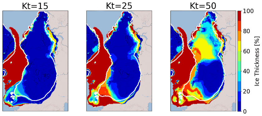
Figure 12 Multi-model mean of the ice thickness loss compared to the initial ice sheet for different basal melting perturbations. LGM ice sheets are built by fixing the basal melting to 0.1 m yr⁻¹ (as in Petrini et al., 2020; Alvarez-Solas et al., 2019). Note that the significant decrease in ice thickness in the Norwegian and Greenland seas is due to the simulation of ice shelves in the new spin-up for the MIROC-ESM forcing (see Fig. S13). These ice shelves are extremely sensitive to a change in the basal melt. The white line indicates the areas where the multi-model mean is done on the five models. K_t is the transfer factor in Eq. (6) (expressed in m yr^{−1 ∘−1}).

Another difference that deserves to be mentioned is that Petrini et al. (2020) used a climatic index based on the transient simulation of Liu et al. (2009). This method ensures that both the atmospheric and oceanic temperatures increase concomitantly up to their pre-industrial levels. As a result, we cannot exclude that the key role of basal melting in their simulated deglaciation is not amplified by the effect of atmospheric warming, which is similar to the conclusions drawn from our EXP4 results.

The second round of sensitivity experiments conducted with new values of climate-related parameters and new parameterizations related to the ice dynamics also confirm the high sensitivity of the EIS to the atmospheric forcing in the GRISLI ice sheet model. This contrasts with the current situation in the West Antarctic ice sheet (WAIS), where ice volume loss is mainly due to melting under the ice shelves (Pritchard et al., 2012). This difference in the response of the two ice sheets raises questions about the mechanisms responsible for their respective evolution.

In addition, WAIS is characterized by large areas of confined ice shelves exerting a buttressing effect on the grounded ice, whereas most of the ice shelves in our simulated LGM EIS are unconfined (see Sect. 4.4.2) However, as temperatures are expected to rise in the future, larger volumes of meltwater will be produced on the surface of the ice shelves (Kittel et al., 2021), potentially favouring the ice shelf disintegration through hydrofracturing (Banwell et al., 2013; Lai et al., 2020). Although this process differs from basal melting, it could bring the WAIS into a similar configuration to the past Eurasian ice sheet.

The ISMIP6 project (Seroussi et al., 2020) shows a significant difference in ice sheet behaviour, depending on the ice sheet model used (Seroussi et al., 2020). Despite the numerous sensitivity experiments presented in this study with various parameter values and different parameterizations of the ice dynamics (see Sect. 4.4), we cannot totally exclude the possible model dependency of our results. To reduce the uncertainties associated with the use of a single ice sheet model, we strongly encourage other ice sheet modellers to perform the same kind of sensitivity tests with several other ice sheet models having, if possible, a higher resolution so as to better capture the fine-scale structure of outlet glaciers and the ice flow dynamics at the grounding line and the marine ice sheet instability.

6 Conclusion

In this paper, we used offline GRISLI2.0 simulations forced by PMIP3/PMIP4 models to investigate the key mechanisms driving the retreat of the Eurasian ice complex at the beginning of the last deglaciation. We paid special attention to the understanding of the processes responsible for the destabilization of the marine-based parts of the Eurasian ice sheets, as GRISLI2.0 includes an explicit calculation of the ice flux at the grounding line, which is expected to account for the representation of the marine ice sheet instability. We first showed that, due to climate biases that are too strong in some GCMs at the LGM, only 5 out of 10 GCMs succeeded in building an ice sheet in agreement with the reconstructions.

The sensitivity experiments have been designed to test the response of the simulated Eurasian ice sheets to surface climate, oceanic temperature, and sea level perturbations. Our results highlight the high EIS sensitivity to a change in surface atmospheric temperatures using the GRISLI model. While basal melting does not seem to be the main driver of the ice sheet retreat, we showed that its effect is clearly amplified by the atmospheric warming.

These results contradict those of previous studies mentioning the central role of the ocean on the deglaciation of BKIS. However, we argue that parts of this disagreement are related to the way the climatic forcing is done (absolute climatic fields, anomalies, or climatic indexes) and the procedure followed for building the initial state of EIS, as well as to the presence of confined or unconfined ice shelves at the LGM. In order to assess the robustness of our analyses, we suggest that other modelling groups reproduce the same kind of sensitivity tests with ice sheet models of a similar or higher complexity. This pluralistic approach would allow us to better understand the uncertainties associated with the ice sheet model used.