Technical note: An improved methodology for calculating the Southern Annular Mode index to aid consistency between climate studies

The Southern Annular Mode (SAM) strongly influences climate variability in the Southern Hemisphere. The SAM index describes the phase and magnitude of the SAM and can be calculated by measuring the difference in mean sea level pressure (MSLP) between middle and high latitudes. This study investigates the effects of calculation methods and data resolution on the SAM index, and subsequent interpretations of SAM impacts and trends. We show that the normalisation step that is traditionally used in calculating the SAM index leads to substantial differences in the magnitude of the SAM index calculated at different temporal resolutions. Additionally, the equal weighting that the normalisation approach gives to MSLP variability at the middle and high southern latitudes artificially alters temperature and precipitation correlations and the interpretation of climate change trends in the SAM. These issues can be overcome by instead using a natural SAM index based on MSLP anomalies, resulting in consistent scaling and variability in the SAM index calculated at daily, monthly and annual data resolutions. The natural SAM index has improved representation of SAM impacts in the high southern latitudes, including the asymmetric (zonal wave-3) component of MSLP variability, whereas the increased weighting given to mid-latitude MSLP variability in the normalised SAM index incorporates a stronger component of tropical climate variability that is not directly associated with SAM variability. We conclude that an improved approach of calculating the SAM index from MSLP anomalies without normalisation would aid consistency across climate studies and avoid potential ambiguity in the SAM index, including SAM index reconstructions from palaeoclimate data, and thus enable more consistent interpretations of SAM trends and impacts.

1 Introduction

The Southern Annular Mode (SAM) is the leading mode of atmospheric variability in the extratropical Southern Hemisphere. The SAM describes changes in the strength and position of the westerly wind belt and associated storm tracks, and can be characterised through the difference in zonal mean sea level pressure (MSLP) between the southern mid-latitudes and Antarctica (Thompson and Wallace, 2000; Marshall, 2003). A positive SAM is characterised by positive pressure anomalies at mid-latitudes and negative pressure anomalies over Antarctica (Fig. 1; Marshall, 2003). These variations in the latitudinal pressure gradient have been found to influence temperature and precipitation across the Southern Hemisphere, and also interact with other major modes of climate variability. For example, a positive SAM has been associated with decreases in precipitation and positive temperature anomalies in south-east South America often as a result of interactions with El Niño–Southern Oscillation (Silvestri and Vera, 2003; Vera and Osman, 2018). In South Africa, a positive SAM is associated with a decrease in rainfall during winter and spring related to a shift in the polar jet (Reason and Rouault, 2005). In Australia, a positive SAM during winter is linked to reduced precipitation in southern parts of the country, while a negative SAM in summer can lead to reduced rainfall and elevated temperature and bushfire risk in parts of eastern Australia (e.g. Meneghini et al., 2007; Mariani and Fletcher, 2016; Lim et al., 2019; Abram et al., 2021). In New Zealand, a positive SAM is linked to a decrease in precipitation and an increase in temperature due to weakened westerly winds passing over the islands (Kidston et al., 2009).

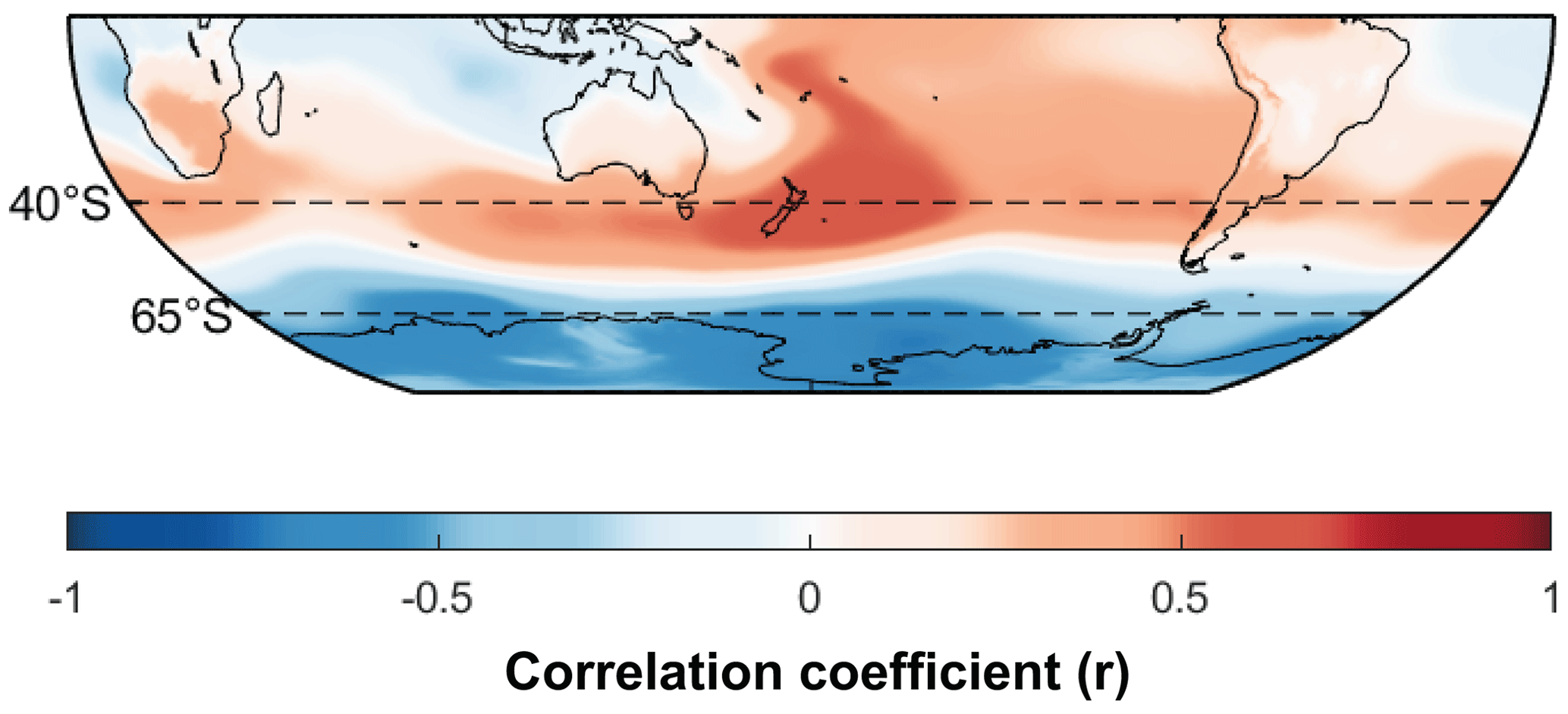
Figure 1 Spatial correlation of SAM index to mean sea level pressure (MSLP) in the Southern Hemisphere. SAM index was calculated from annually means (January–December; 1950–2022, ERA5 data) using the difference in zonal MSLP at 40 and 65° S (dashed lines).

The phase and magnitude of SAM variability is described by the SAM index. Two methods are commonly used to calculate the SAM index. The first method is based on gridded data such as atmospheric reanalysis (e.g. ERA5) or climate model output, and breaks down extratropical Southern Hemisphere atmospheric pressure data into orthogonal spatial patterns expressed by empirical orthogonal functions (EOFs). The first EOF explains the leading mode of Southern Hemisphere variability and its time series represents the SAM index (Mo, 2000; Fogt and Bromwich, 2006). Recent advances in the application of the EOF method to describe the SAM include approaches to separate the zonally symmetric component of SAM variability from the asymmetric component of variability associated with the zonal wave-3 pattern (Goyal et al., 2022; Campitelli et al., 2022). The second method for calculating the SAM index uses the difference in the normalised zonal mean sea level pressure (MSLP) between 40 and 65° S (Fig. 2). By this method the SAM index can be calculated using gridded products from reanalysis or model outputs (Gong and Wang, 1999) or from more sparse instrumental records of MSLP from observing stations located in the southern mid-latitudes and around coastal Antarctica (Marshall, 2003). It is this second method of calculating the SAM index that is the main focus of the assessment carried out in this study; however, we do also demonstrate the extension of our findings to EOF-based methods.

Instrumental climate measurements are sparse across the Southern Hemisphere, and particularly in Antarctica. This generally limits a reliable long-term understanding of SAM variability from observations and reanalysis products to the time since 1957 (Marshall, 2003; Barrucand et al., 2018; Marshall et al., 2022), although some longer reconstructions based on observations have also been developed back to the late 19th century (Jones et al., 2009; Visbeck, 2009). Over this historical period there has been a significant positive trend in the SAM, particularly in the summer season, associated with stratospheric ozone loss as well as rising atmospheric greenhouse gases (Thompson and Solomon, 2002; Fogt and Marshall, 2020). This trend is expected to continue in all seasons during the 21st century as climate continues to warm due to ongoing anthropogenic greenhouse gas emissions but with a temporary pause in summer trends due to the opposing influence of stratospheric ozone recovery (Thompson et al., 2011; Goyal et al., 2019; Banerjee et al., 2020)

Longer-term reconstructions of the SAM have been developed using palaeoclimate proxy records (e.g. ice cores, tree rings and corals) and multiple reconstructions for the last millennium have been produced (e.g. Villalba et al., 2012; Abram et al., 2014; Dätwyler et al., 2018; King et al., 2023). These long-term reconstructions show similar trends in the SAM index; however, they display different magnitudes of reconstructed SAM variability. Although variability between reconstructions could be due to differences in reconstruction methods and the networks of proxy data used, Wright et al. (2022) instead found that differences in magnitude between the Abram et al. (2014) and Dätwyler et al. (2018) reconstructions were explained by the data resolution used to calculate the instrumental SAM index. Dätwyler et al. (2018) trained their reconstruction to an annual SAM index calculated from monthly MSLP data, while Abram et al. (2014) used the annual SAM index from annual MSLP data as their reconstruction target. The difference in magnitude of the annual SAM index in instrumental data calculated by these alternate methods accounts for the apparently larger (though dimensionless) magnitude of SAM variability during the last millennium in the Abram et al. (2014) reconstruction compared with the Dätwyler et al. (2018) reconstruction (Wright et al., 2022). This discrepancy highlights the importance of understanding the impact of methodology in reconstructing the SAM index from observational data.

It has previously been shown that differences between the method (e.g. EOF or zonal difference index methods), variable (e.g. pressure level) or source data (e.g. gridded reanalysis or station observations) result in sometimes marked differences between available observational SAM indices, despite these indices all representing the same physical process (Ho et al., 2012). However, it is not known how methodological choices within a single method, variable and data source might also have the potential to influence the results of SAM studies. To date, an optimal data resolution to use when calculating the SAM index has not been established, and various versions constructed using different resolutions and orders of operation are made available for the research community to use (e.g. http://www.nerc-bas.ac.uk/icd/gjma/sam.html, last access: 17 May 2023). It also remains unexplored if the choice to normalise zonal MSLP data prior to calculating the latitudinal difference in pressure anomalies (Gong and Wang, 1999; Marshall, 2003) could influence assessments of past and future SAM changes or the climate impacts that SAM causes in different parts of the Southern Hemisphere.

Here, we calculate historical SAM indices using daily, monthly and annual averages of zonal MSLP data and using normalised (traditional) and natural formulations of the SAM index. We explore differences between the SAM indices and the reasons why methodological choices introduce these differences, as well as the potential implications when analysing the spatial correlation of SAM variability with temperature and precipitation impacts. Additionally, we also explore the influence of methods on the interpretation of SAM trends in projections of climate change during the 21st century. We conclude by making recommendations for an improved approach to calculating the SAM index that avoids potential differences introduced by methodology.

2 Methods

We use the ECMWF (European Centre for Medium-Range Weather Forecasts) Reanalysis v5 (ERA5) gridded data for our study (Hersbach et al., 2020). ERA5 reanalysis data are currently available from 1950. Of the available reanalysis products, ERA5 has been shown to best reproduce Antarctic surface temperature and SAM relationships prior to the satellite era (Marshall et al., 2022).

Daily resolution MSLP data in ERA5 for latitudes 40 and 65° S were sourced from the KNMI Climate Explorer tool (Trouet and Van Oldenborgh, 2013). From daily ERA5 data, the daily, monthly and annual means of zonal MSLP were calculated. SAM indices were then calculated for these three different data resolutions (Fig. 2).

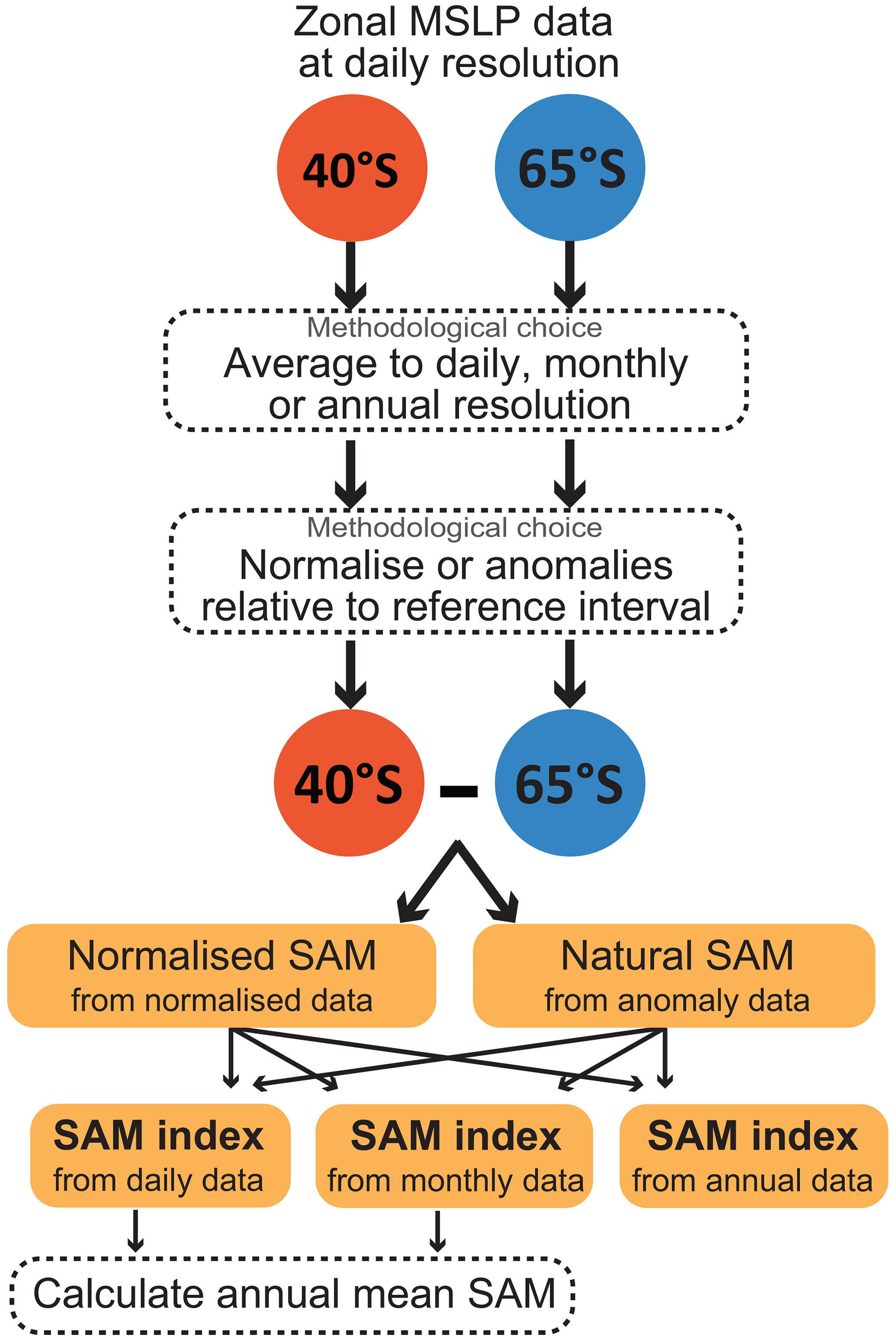
Figure 2 Methodological choices explored in this study by calculating normalised and natural SAM indices from different data resolutions.

Following the approach of Gong and Wang (1999), the SAM index was first calculated using the following equation:

$$\begin{array}{}\text{(1)}& \mathrm{SAM}=P_{\mathrm{40}\mathit{°}\mathrm{S}}^{*}-P_{\mathrm{65}\mathit{°}\mathrm{S}}^{*},\end{array}$$

where $P_{\mathrm{40}\mathit{°}\mathrm{S}}^{*}$ and $P_{\mathrm{65}\mathit{°}\mathrm{S}}^{*}$ are the normalised zonal MSLP at 40 and 65° S respectively.

Data was normalised relative to a 1961–1990 reference interval. Briefly, this involves subtracting the mean of the reference interval from the time series, and then dividing the time series by the reference interval standard deviation. The SAM index was then calculated by subtracting the normalised zonal MSLP values at 65° S from the normalised zonal MSLP values at 40° S (Fig. 2). The normalisation step removes units from the MSLP data, and consequently the resultant SAM index is also dimensionless. We refer to this as the normalised SAM index.

A natural SAM index in pressure units of hPa was also calculated (Fig. 2). This followed the same equation and method as above, but in this case $P_{\mathrm{40}\mathit{°}\mathrm{S}}^{*}$ and $P_{\mathrm{65}\mathit{°}\mathrm{S}}^{*}$ are the zonal MSLP anomalies at 40 and 65° S. Specifically, for the natural SAM index the zonal MSLP anomalies are calculated relative to the 1961–1990 reference interval mean without dividing by the reference interval standard deviation.

Discrepancies between daily, monthly and annual SAM index methods were investigated by calculating an annual mean SAM from the daily and monthly indices (Fig. 2). The annual SAM values derived from the different resolution SAM indices were then compared by a correlation coefficient (r) and by examining the gradient between different methods of calculating the SAM index. The spatial correlation of each SAM index at each data resolution with ERA5 gridded data for 2 m air temperature and precipitation was also examined to test the influence of methodological choices on detection and interpretation of the SAM's climate impacts.

To illustrate the impact that methodological choices could have on the interpretation of future SAM changes we also test climate model output from 1850 to 2100. To illustrate the effect of methodological choices we use output from the CSIRO ACCESS-CM2 model prepared for CMIP6 (Dix et al., 2019). A full assessment of future SAM changes would require a more thorough analysis across the ensemble of CMIP6 models, as done for example in Goyal et al. (2021), but our purpose in this study is to simply illustrate the potential impact of methodological choices on such assessments. MSLP outputs from the ACCESS-CM2 model were sourced from the “very high” and “low” emission scenarios for future climate change (SSP5-8.5 and SSP1-2.6 respectively) in order to best identify the range of influences that methodological choice could have on assessing SAM changes in a warming climate. As the output from these global climate model simulations are routinely reported at monthly mean resolution, only monthly and annual mean SAM indices were calculated for the future projections. Both normalised and natural SAM indices were calculated from the climate model output, relative to a 1961–1990 reference interval.

In addition to these main analyses, we also verify the broad application of our findings by repeating our calculations of normalised and natural SAM indices using the station locations that are used for the Marshall SAM index (Marshall, 2003). For this we used the ERA5 MSLP data extracted for the 12 grid cells corresponding to the station locations used for the Marshall SAM index (Marshall, 2003). We further extended our comparison across common SAM index methodologies by constructing EOF-based SAM indices using the ERA5 gridded MSLP data from south of 20° S at monthly and annual resolutions.

All data analysis were carried out using MATLAB R2022b software. This included using the M-map package and the Climate Data Toolbox for producing the analyses and maps presented in this study (Greene et al., 2019; Pawlowicz, 2020).

3 Results

3.1 SAM index characteristics

Data resolution strongly influences the magnitude of the normalised SAM index (Fig. 3a). While the pattern of interannual variability in the normalised SAM is very similar for all data resolutions (as demonstrated by r values exceeding 0.99; Fig. 3b–c), the magnitude of interannual variability in the normalised SAM derived from monthly data is 1.4 times larger than the normalised SAM derived from daily data (Fig. 3b). Similarly, the magnitude of the annual normalised SAM index calculated from annual means is 3.1 times larger than the normalised SAM derived from monthly data (Fig. 3c) and 4.4 times higher than the annual SAM derived from daily data. This finding is consistent with the recalculation performed by Wright et al. (2022), where the SAM index calculated from annual MSLP data displayed a higher variability than annual means derived from a monthly SAM index.

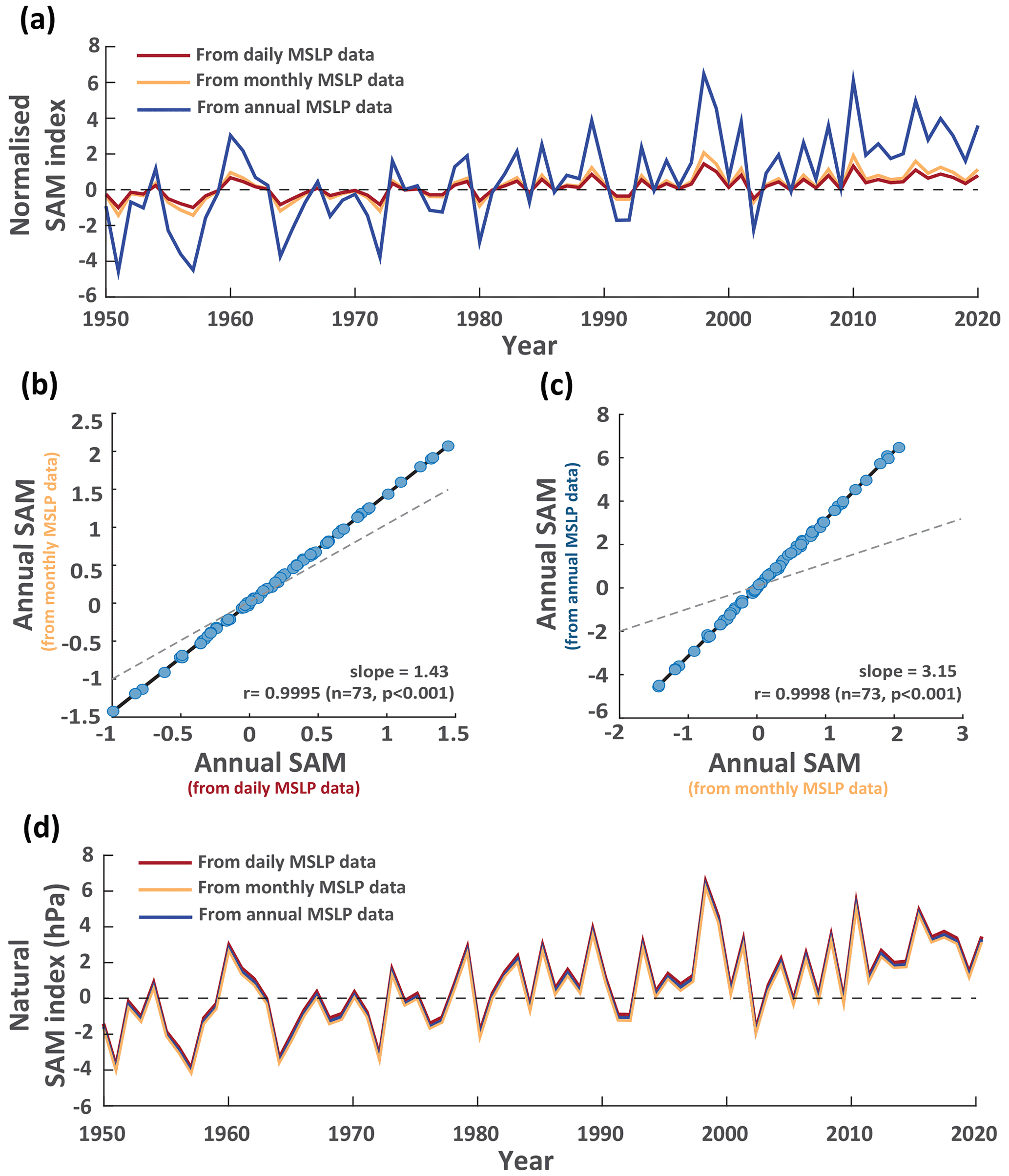
Figure 3 Annual mean SAM values calculated by different methodological choices. (a) Comparison of annual normalised SAM values calculated from daily (red), monthly (orange) and annual (blue) MSLP data. (b) Relationship between the annual normalised SAM values calculated from daily and monthly resolution MSLP data. Dashed line represents 1:1 slope (c) Relationship between the annual normalised SAM values calculated from monthly and annual resolution MSLP data. Dashed line represents 1:1 slope. (d) Comparison of annual natural SAM values calculated from daily (red), monthly (orange) and annual (blue) MSLP data.

Differences in magnitude of the normalised SAM index are caused by a progressive decrease in standard deviation as MSLP data are averaged over longer time periods (Table 1). This means that the normalisation of daily MSLP data removes a larger magnitude of variability than normalisation of monthly MSLP data, and even more so when comparing to normalisation of annual resolution MSLP data. Comparison of the reference interval MSLP standard deviations between the different data resolutions (Table 1) gives similar ratios to the slopes between the annual mean SAM values derived from different resolution SAM indices in Fig. 3a–c. For example, the normalisation step in calculating the SAM index removes a 3.3 times greater magnitude of MSLP variability at 40° S for monthly resolution data compared to annual mean data (standard deviations of 1.694 and 0.509 hPa respectively; Table 1), and 3 times more variability at 65° S (standard deviations of 4.025 and 1.355 hPa respectively; Table 1). This results in the 3.1 times greater magnitude of interannual SAM variability calculated from annual data relative to monthly data when using the normalisation method to calculate the SAM index (Fig. 3c).

Differences in the magnitude of the SAM index are overcome when a natural SAM index is instead calculated. The annual mean natural SAM values calculated from daily, monthly and annual resolution MSLP data all display a near-identical magnitude of interannual variability over time (Fig. 3d). This highlights how the normalisation step that is traditionally used in calculating the SAM index can introduce ambiguity into SAM studies but also how this ambiguity can be avoided by retaining the native pressure units in the natural SAM index.

Our findings also demonstrate that a natural SAM index can be reliably calculated from low-resolution MSLP data. Physically, it is the instantaneous difference in pressure between the middle and high southern latitudes that represents the processes of atmospheric SAM variability (Baldwin, 2001), and so daily resolution data might be assumed to retain a more pure measure of the SAM index. However, our findings using different resolutions of MSLP data show that the interannual trends and variability in the natural SAM are consistently captured using daily, monthly or annually averaged zonal MSLP anomalies (Fig. 3d).

Our findings for the SAM index derived from the latitudinal pressure difference in gridded MSLP data also extend to other methods of calculating the SAM index. Consistent findings with those demonstrated in Fig. 3 are produced when normalised and traditional SAM indices are produced using the 12 observational locations used for the Marshall SAM index (Fig. A1). Similarly, the annual SAM data produced using an EOF method applied to monthly resolution gridded MSLP data have a muted amplitude compared to the same EOF-derived index based on annual resolution data (Fig. A2). This demonstrates how the normalisation process impacts the scaling of the SAM index derived from different temporal resolutions of input data regardless of the SAM index method used.

Beyond scaling, there are additional (though small) year-to-year differences in the interannual variability and trends of the SAM when comparing natural and normalised calculations of the SAM index. These differences are evident when comparing annual SAM values calculated as a natural or normalised index from annual MSLP data (Fig. 4, Table A1) and are similarly evident when comparing the variability in natural and normalised SAM indices calculated from monthly MSLP data or from daily MSLP data (Table A1).

These differences in year-to-year variability and trends can again be explained as an artefact introduced by the normalisation step when calculating the traditional SAM index. By normalising the zonal MSLP data before calculating the zonal difference, an identical weighting is given to pressure variability in the middle and high latitudes in the calculation of the normalised SAM index. However, the magnitude of MSLP variability is consistently larger at 65° S compared with 40° S (Table 1). At daily resolution, the magnitude of reference interval variability at 65° S is 2.22 times larger than the variability at 40° S (standard deviations of 5.597 and 2.524 hPa respectively), and at annual resolution, variability at 65° S is 2.66 times larger than at 40° S (standard deviations of 1.355 and 0.509 hPa respectively). Likewise, the long-term trends in MSLP are amplified at 65° S (−0.50 hPa per decade from 1950–2022) compared to the MSLP trends at 40° S (0.18 hPa per decade). These differences suggest that the equal weighting of these latitudinal zones that is routinely applied in calculating the normalised SAM index may not be justified and could artificially alter the interpretation of SAM variability, trends and impacts.

Table 1 Characteristics of MSLP variability during the 1961–1990 reference interval for the zonal MSLP data used to calculate the SAM index at different resolutions.

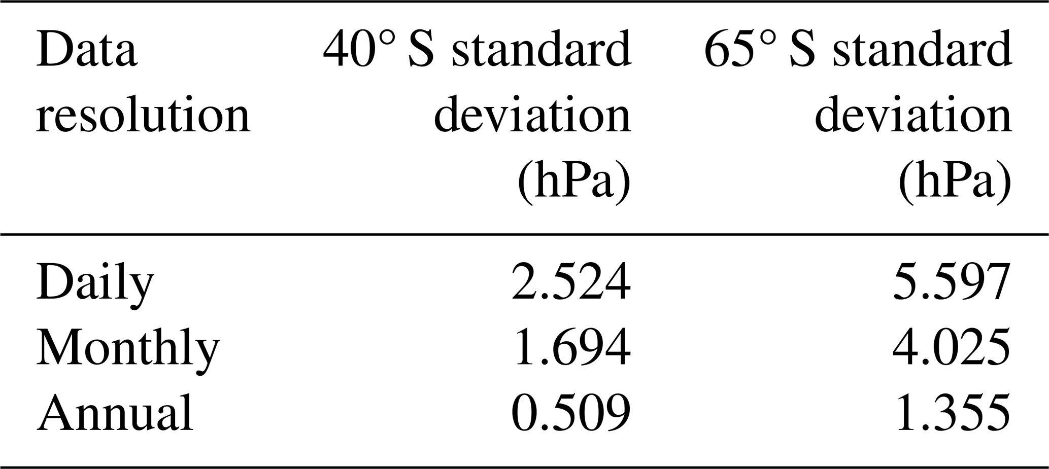
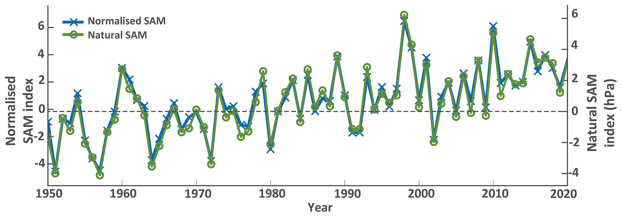
Figure 4 Comparison of interannual variability and trends from normalised and natural annual SAM values calculated from annual resolution MSLP data. y-axis limits have been scaled relative to the regression slope between the natural and normalised SAM index to provide the optimal alignment of the indices.

3.2 SAM impacts

Spatial correlation analysis shows that the SAM index is correlated with Southern Hemisphere temperature variability, with similar broad-scale patterns across SAM index data resolutions and calculation methods (Fig. 5). In general, all formulations of the SAM indices produce negative correlations with annual mean temperature anomalies over the Antarctic continent and positive correlations over the Antarctic Peninsula and southern South America, over the southern Indian Ocean and over the Maritime continent extending into the eastern tropical Indian Ocean, the Coral Sea and the Tasman Sea. However, beyond these broadly consistent patterns we demonstrate that the methodology used to construct the SAM index does alter the strength of temperature correlations in some locations.

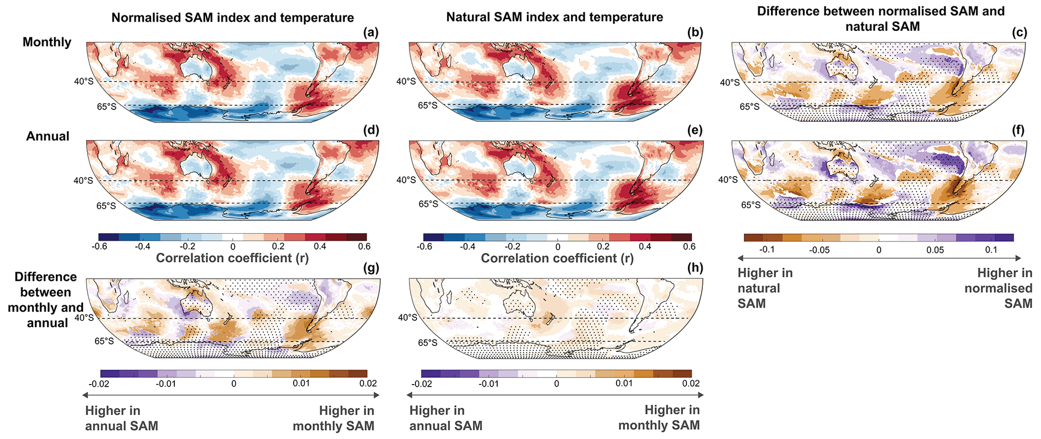
Figure 5 Spatial correlation of annual SAM values with ERA5 2 m air temperature in the Southern Hemisphere (January–December averages over 1950–2022). Comparisons are shown for differences in SAM indices derived from monthly (a, b) and annual (d, e) MSLP data for normalised SAM indices (a, d) and natural SAM indices (b, e). Also shown are the differences in spatial correlation values based on MSLP data resolution (g, h) and for natural versus normalised SAM indices (c, f). In these correlation difference plots, the shading represents differences between methods and data resolution while stippling indicates regions of negative spatial correlations. Consistent findings are also produced comparing annual temperature correlations for SAM indices derived from daily and annual MSLP data (Fig. A3).

Comparing the correlations produced by normalised versus natural formulations of the SAM index (i.e. comparing columns in Fig. 5), clear spatial characteristics in correlation differences are evident. Generally, correlation strength in the region between 40 and 65° S is stronger for the natural SAM than it is for the normalised SAM. These differences in correlation strength show three distinct nodes across the Southern Ocean and Drake Passage, suggesting that the natural SAM index better includes the asymmetric (zonal wave-3) component of SAM variability. In contrast, areas north of 40° S more commonly have stronger correlations with the normalised SAM index. It is expected that this is because the normalised SAM index artificially increases the weighting of MSLP variability at 40° S (relative to MSLP variability at 65° S). This emphasises the temperature effects of pressure variability in the mid-latitudes as well as their interactions with tropical circulation such as the Hadley and Walker circulation cells.

Two important features are found when comparing the annual temperature correlations produced by different resolutions of the SAM index (i.e. comparing rows in Fig. 5). Firstly, differences in resolution of the normalised SAM produce similar spatial patterns of correlation differences as are seen in the comparison between natural and normalised SAM indices. Specifically, the normalised SAM generated from monthly resolution MSLP data has stronger correlations with interannual temperature variability in the region between 40 and 65° S, including showing improved correlation with the zonal wave-3 pattern. The normalised SAM generated from annual resolution MSLP data has generally stronger correlations with interannual temperature variability north of 40° S. These differences are emphasised even further in comparing annual temperature correlations with the normalised SAM generated from daily versus annual MSLP data (Fig. A3). This is again explainable through the increasingly strong weighting that is given to pressure variability at 40° S relative to variability at 65° S as MSLP data resolution is reduced in calculating the normalised SAM (Table 1). However, the other important finding that is evident in this analysis is that the spatial differences in correlation strength associated with MSLP data resolution can be avoided almost altogether by using a natural SAM index (middle column of Fig. 5).

Similar findings come from examining the correlation of annual precipitation with the various methodological choices for calculating the SAM index (Fig. 6). The primary correlation patterns with precipitation show broad agreement across methods. Positive mean annual SAM anomalies are associated with latitudinal bands of increased precipitation near the Antarctic coast (including over the Antarctic Peninsula) and a band of decreased precipitation across the mid-latitudes. This represents the southward shift of the westerly winds and associated storm tracks when the SAM is in its positive phase. Other regions demonstrating positive mean annual precipitation associated with positive SAM anomalies include the Maritime Continent including the eastern tropical Indian Ocean and eastern Australia and the tropical eastern and central Pacific. Negative mean annual precipitation anomalies are also seen over West Antarctica in response to positive SAM phases.

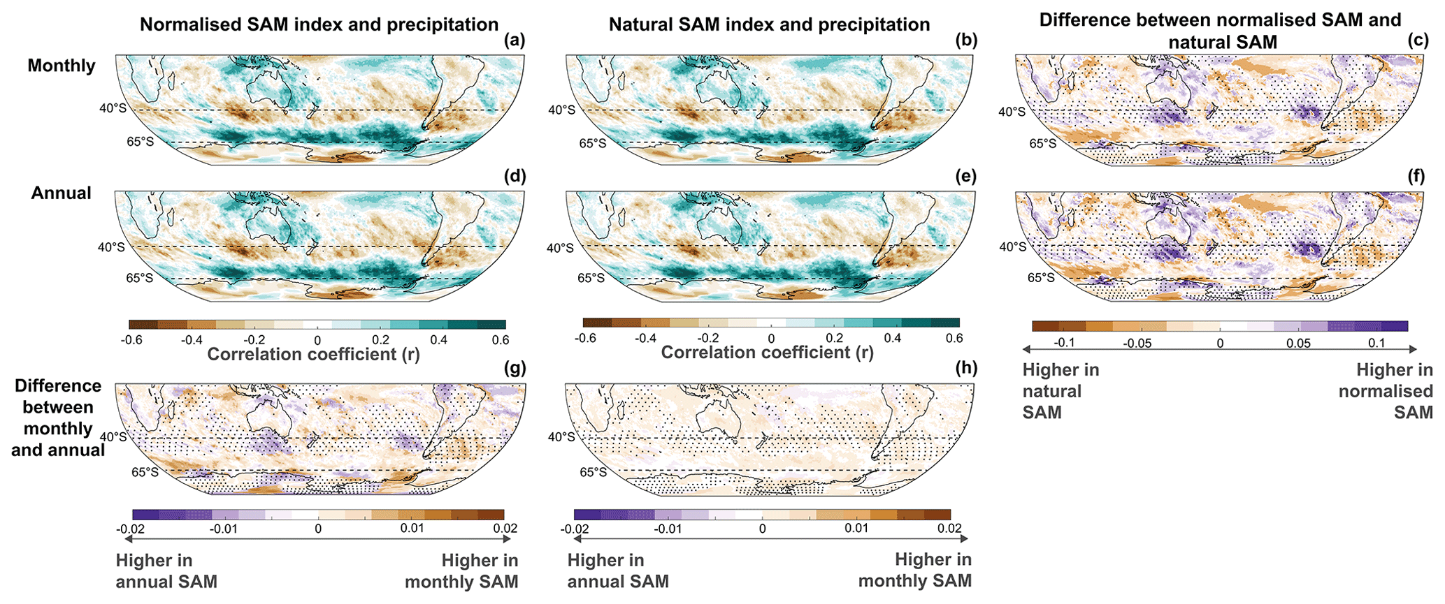
Figure 6 Spatial correlation of annual SAM values with ERA5 precipitation in the Southern Hemisphere (January–December averages over 1950–2022). Comparisons are shown for differences in SAM indices derived from monthly (a, b) and annual (d, e) MSLP data for normalised SAM indices (a, d) and natural SAM indices (b, e). Also shown are the differences in spatial correlation values based on MSLP data resolution (g, h) and for natural versus normalised SAM indices (c, f). In these correlation difference plots, the shading represents differences between methods and data resolution while stippling indicates regions of negative spatial correlations. Consistent findings are also produced comparing annual precipitation correlations for SAM indices derived from daily and annual MSLP data (Fig. A4).

Beyond these broad similarities in SAM correlations with precipitation, we do again identify regions where methodological choices alter the correlation results produced (Figs. 6, A4). Correlations with interannual precipitation variability near 65° S, and particularly over the Antarctic Peninsula, are generally stronger for higher-resolution versions of the normalised SAM index and for all resolutions of the natural SAM index. Conversely, correlations with interannual precipitation variability near 40° S, and specifically south of Australia, over the South Island of New Zealand and west of Chile, are stronger for lower-resolution versions of the normalised SAM and for the normalised SAM compared with the natural SAM. These formulations of the SAM index also show stronger precipitation anomalies over parts of the tropics including northern Australia and the Amazon region, indicating the stronger representation of tropical-to-mid-latitude atmospheric circulation in these versions of the SAM index that give increased weighting to pressure anomalies at 40° S. In other words, it is these regions where methodological choices in constructing the SAM index will have the most impact on the interpretation of the SAM’s influence on annual mean precipitation.

We note that these comparisons are shown for mean annual precipitation and SAM anomalies, but it is well established that the impacts of SAM on precipitation vary by season (Fogt and Marshall, 2020). Because of this, the impacts of methodological choices in assessing the SAM’s precipitation impacts at a seasonal scale may result in different regions where those methodological choices alter correlation strength. However, we expect that our general conclusions would remain the same at the seasonal scale, including that a natural version of the SAM index would produce correlation results that are unaffected by choices in the resolution of zonal MSLP data used to construct the SAM index.

3.3 SAM trends

Finally, we look at how methodological choices in constructing the SAM index could alter the interpretation of SAM changes in a warming world. During the historical period the differences in interannual variability in annual SAM values produced by natural or normalised SAM indices are detectable but small (Fig. 4). However, as the response to human-caused climate warming develops, the magnitude of SAM trends relative to the magnitude of historical variability show increasing differences between different methodological versions of the SAM index (Fig. 7).

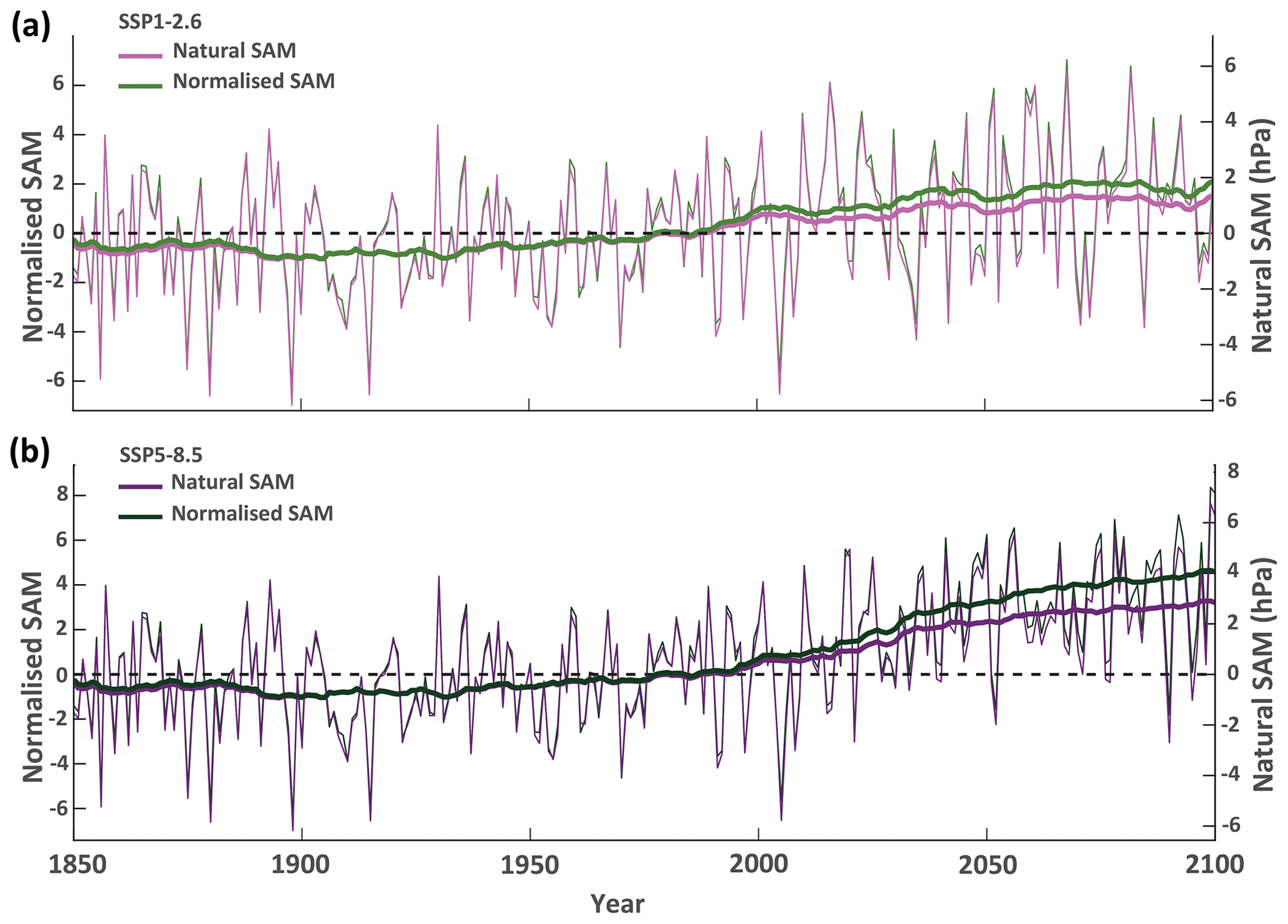
Figure 7 Example of future scenario SAM indices based on different calculation methods. (a) Comparison of a low-emissions future scenario (SSP1-2.6) based on natural (purple) and normalised (green) SAM indices calculated from annual MSLP data for 1850–2100. Thick lines show 50-year moving averages. Reference interval used for calculating the SAM indices is 1961–1990. (b) As in (a) but for a very-high-emissions future scenario (SSP5-8.5). y-axis limits have been scaled relative to the regression slope between the natural and normalised SAM index over the reference interval to provide the optimal alignment of the indices.

Long-term climate change trends are stronger in the normalised SAM compared to the natural SAM, relative to historical interannual variability (Fig. 7). This difference will affect interpretations of time of emergence (Hawkins et al., 2020), which assess when a long-term climate trend (signal) emerges above the amplitude of historical climate variability (noise) resulting in climate conditions that are beyond the range of historical experience. For example, under a future with very high greenhouse gas emissions (SSP5-8.5) the climate change signal on the SAM index (as assessed by a 50-year moving average) emerges above the 1 standard deviation historical (1850–1949) noise level by 2025 and above the 2 standard deviation historical noise level by 2091, in a normalised formulation of the SAM. In contrast, for the natural SAM there is emergence above the 1 standard deviation level by 2031, but no emergence occurs above the 2 standard deviation level during the 21st century. Likewise, under a low greenhouse gas emissions scenario (SSP1-2.6) there is emergence of the climate change signal for the normalised SAM between 2063 and 2086, but emergence is not detected at any time during the 21st century for the natural SAM.

This finding illustrates how methodological differences in calculating the SAM index have the potential to alter interpretations of human-caused climate impacts on the SAM. Our findings suggest that the normalised SAM index may lead to assessments that the SAM has emerged outside of the range of historical experience sooner than would be determined based on a natural SAM index. We emphasise that this is only an illustrative example based on a single climate model, but it does demonstrate the potential for methodological choices to influence the interpretation of SAM trends between different studies.

4 Discussion and Conclusions

Our results allow us to make recommendations for an improved approach to calculating the SAM index that can enable greater consistency across climate studies. The traditionally used (normalised) SAM index (Gong and Wang, 1999; Marshall, 2003) involves normalising zonal MSLP data before calculating the latitudinal MSLP difference that defines the SAM. It is not clear why the choice to normalise zonal MSLP data was originally made, although it is possible that this was to align with EOF-based methods of defining the SAM that produce non-dimensional principal components (Gong and Wang, 1999; Baldwin, 2001), to allow each latitude to contribute equally to the index, or because of the scarcity of observations and potential spurious trends in early MSLP data in the Antarctic region (Baldwin, 2001; Marshall, 2003). It is possible that biases between different climate model representations of atmospheric pressure fields in the Southern Hemisphere might also be somewhat avoided through applying normalisation in constructing the SAM index.

We find that the normalisation step involved in the traditionally defined SAM index has the potential to introduce multiple discrepancies in climate studies. Firstly, the magnitude of the normalised SAM index value varies substantially based on the temporal resolution of zonal MSLP data used to construct the SAM index (Fig. 3a–c). Because the index produced by this method is dimensionless, these differences are hard to trace when SAM indices are then applied in climate research, and there are examples where this has then resulted in seemingly large differences in the magnitude of palaeoclimate reconstructions of the SAM (Wright et al., 2022). The normalisation step also gives equal weighting to MSLP variability and trends in the middle and high latitudes. However, the magnitude of MSLP variability and trends are substantially larger at 65° S compared to 40° S (Table 1). The effect of equally weighting MSLP anomalies at 40 and 65° S results in differences in correlations with temperature and rainfall data that could alter the interpretation and attribution of SAM impacts in some regions. This includes generally reducing SAM correlations with temperature and precipitation variability in the high southern latitudes and giving enhanced influence to the impacts of mid-latitude pressure anomalies and their links to tropical atmospheric circulation (Figs. 5 and 6). Furthermore, the normalised SAM index displays stronger future climate change trends relative to the magnitude of historical variability. Because of this, the SAM would be assessed to emerge above historical experience sooner this century using a normalised SAM index compared with a natural index (Fig. 7).

These problems are overcome when using a natural version of the SAM based on zonal MSLP anomalies rather than normalised MSLP data. The natural SAM index produces consistent indices across different resolutions of MSLP data (Fig. 3d) that also have consistent spatial correlations with temperature and precipitation (Figs. 5 and 6). Although SAM index anomalies are commonly expressed in monthly, seasonal or yearly means, it is the influence of the SAM on synoptic-scale features such as the path of low-pressure system storms and Rossby wave breaking that determines climate impacts (Pepler, 2020; Spensberger et al., 2020). This might suggest that accurate representation of the SAM requires daily or better resolution of MSLP data. However, we demonstrate that the annually averaged climate impacts of the SAM are as effectively represented by latitudinal differences in annual MSLP data as they are for monthly or daily resolution MSLP data (Figs. 5 and 6; A3 and A4), provided that a natural SAM index method is used. Correlations of temperature and precipitation anomalies with the SAM are also consistently stronger for the mid-to-high-latitude region where SAM variability is focused when using the natural SAM compared with the normalised SAM. This includes an improved representation of the asymmetric (zonal wave-3) components of SAM variability in the natural SAM index, whereas increased weighting of mid-latitude pressure anomalies in the normalised SAM results in increased incorporation of tropical atmospheric circulation anomalies into the SAM index.

Discrepancies in the normalised SAM index appear to be related to the assumed equal weighting of MSLP variability at the middle and high latitudes when the zonal MSLP data are normalised. Instead of assuming either equal (normalised SAM) or no weighting (natural SAM) of zonal MSLP data, it could be considered if an equal area weighting based on latitude is optimal for constructing the SAM index. This latitudinal weighting can be achieved by multiplying the zonal MSLP data by the square root of the cosine of latitude (resulting in a weighting of 0.875 for 40° S and 0.650 for 65° S). This latitudinal weighting has a ratio of 1.3, which is substantially less than the observed difference in MSLP variability and trends which are approximately 2–3 times larger at 65 than 40° S (Table 1). Hence, even when accounting for equal area, the variability and trends in MSLP data remain larger at 65° S and should therefore provide a larger contribution to SAM variability than pressure variability at 40° S (Table A2). This is further verified by repeating our analyses using a natural SAM index based on latitude-weighted MSLP data. These demonstrate that spatial temperature and precipitation correlations are stronger for the natural SAM rather than a weighted natural SAM (Figs. A5–A6). The weighted natural SAM also has spatial correlation differences when the SAM is calculated at different temporal resolutions which are not present for the natural SAM (Figs. A5–A6). Hence it appears that area weighting of MSLP anomalies does not improve the representation of the SAM index.

We thus recommend that an improved method for calculating the SAM index from zonal MSLP data should be

$$\begin{array}{}\text{(2)}& \mathrm{SAM}=P_{\mathrm{40}\mathit{°}\mathrm{S}}^{*}-P_{\mathrm{65}\mathit{°}\mathrm{S}}^{*},\end{array}$$

where $P_{\mathrm{40}\mathit{°}\mathrm{S}}^{*}$ and ${}_{\mathrm{65}\mathit{°}\mathrm{S}}^{*}$ are the zonal MSLP anomalies at 40 and 65° S respectively.

Using this method, the resulting natural SAM index will have dimensional pressure units that avoid scaling issues and ambiguity between studies, give appropriate influence to different magnitude of pressure anomalies between the mid-latitudes and Antarctica, produce consistent indices and spatial correlation results across temporal scales and generate generally stronger relationships to SAM impacts in the southern high latitudes than the traditionally used normalised SAM index.

Appendix A

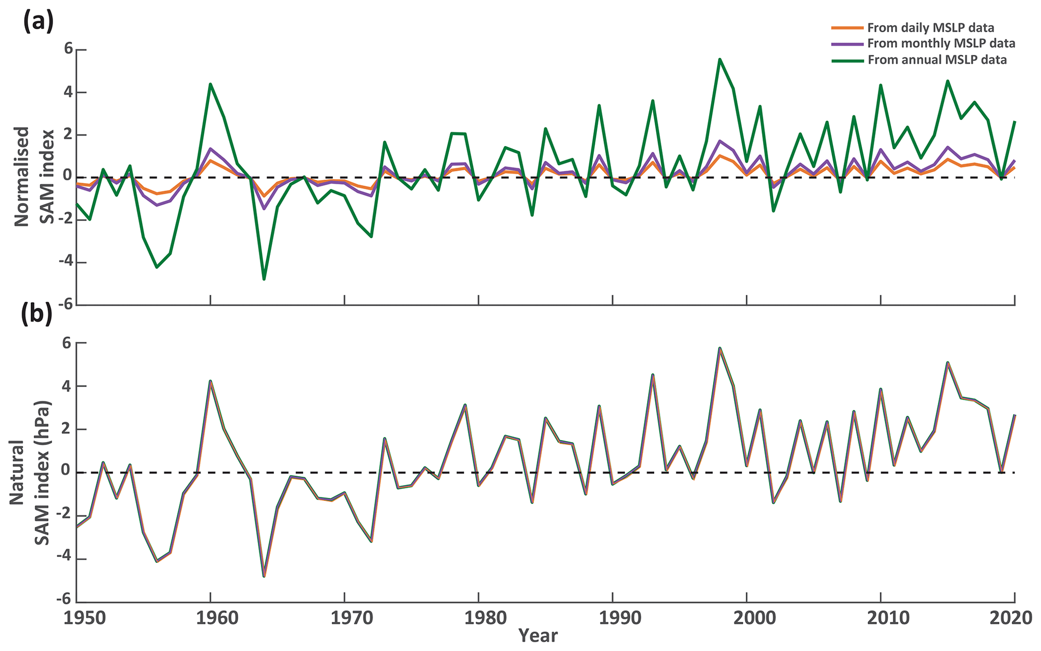
Figure A1 Annual mean SAM values calculated from station sites used in the Marshall index by different methodological choices. (a) Comparison of annual normalised SAM values calculated from daily (orange), monthly (purple) and annual (green) MSLP data. (b) Comparison of annual natural SAM values calculated from daily (orange), monthly (purple) and annual (green) MSLP data.

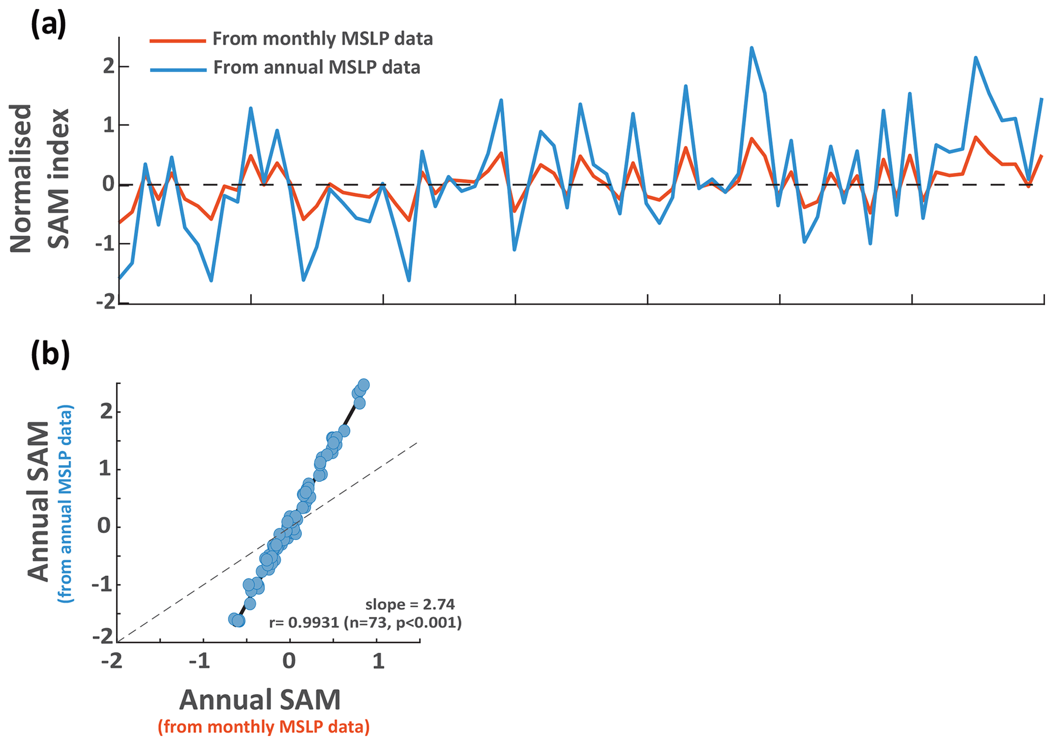
Figure A2 Annual mean SAM values calculated using the EOF method. (a) Comparison of annual SAM values calculated from monthly (orange) and annual (blue) MSLP data. (b) Relationship between the annual SAM values calculated from monthly and annual resolutions MSLP data. Dashed line represents 1:1 slope.

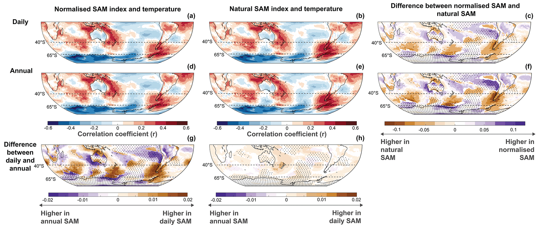
Figure A3 Spatial correlation of annual SAM values with ERA5 2 m air temperature in the Southern Hemisphere (January–December averages over 1950–2022). Comparisons are shown for differences in SAM indices derived from daily (a, b) and annual (d, e) MSLP data and for normalised SAM indices (a, d) and natural SAM indices (b, e). Also shown are the differences in spatial correlation values based on MSLP data resolution (g, h) and for natural versus normalised SAM indices (c, f). In these correlation difference plots, the shading represents differences between methods and data resolution while stippling indicates regions of negative spatial correlations.

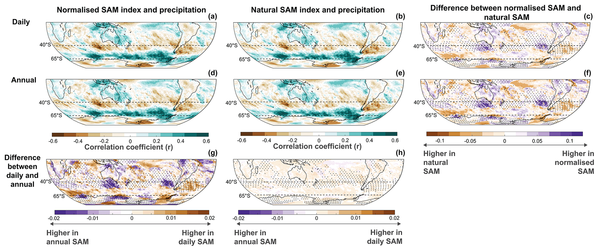
Figure A4 Spatial correlation of annual SAM values with ERA5 precipitation in the Southern Hemisphere (January–December averages over 1950–2022). Comparisons are shown for differences in SAM indices derived from daily (a, b) and annual (d, e) MSLP data and for normalised SAM indices (a, d) and natural SAM indices (b, e). Also shown are the differences in spatial correlation values based on MSLP data resolution (g, h) and for natural versus normalised SAM indices (c, f). In these correlation difference plots, the shading represents differences between methods and data resolution while stippling indicates regions of negative spatial correlations.

Table A1 Correlation coefficients and slopes between data resolutions between calculation methods.

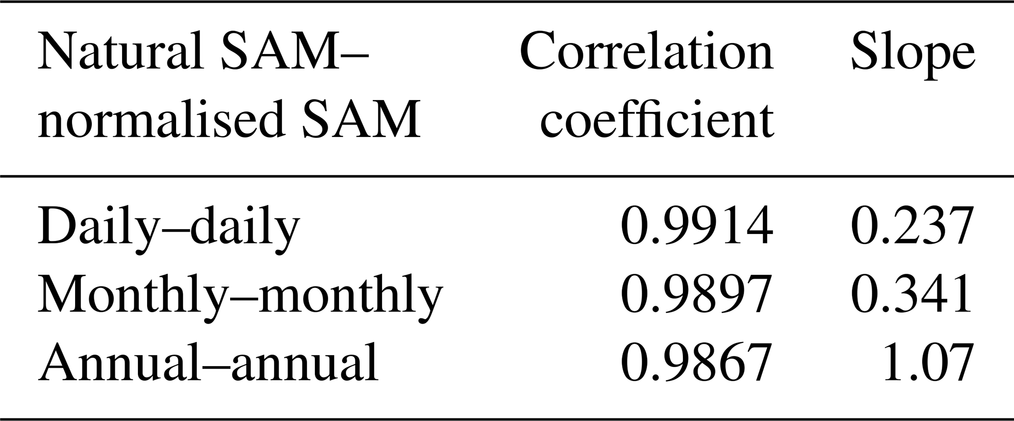
Table A2 Characteristics of latitude-weighted MSLP variability and trends for the zonal means used to calculate the SAM index at different data resolutions.

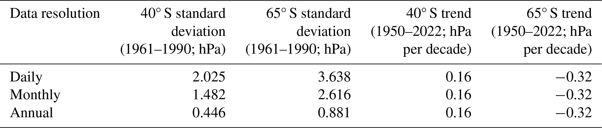
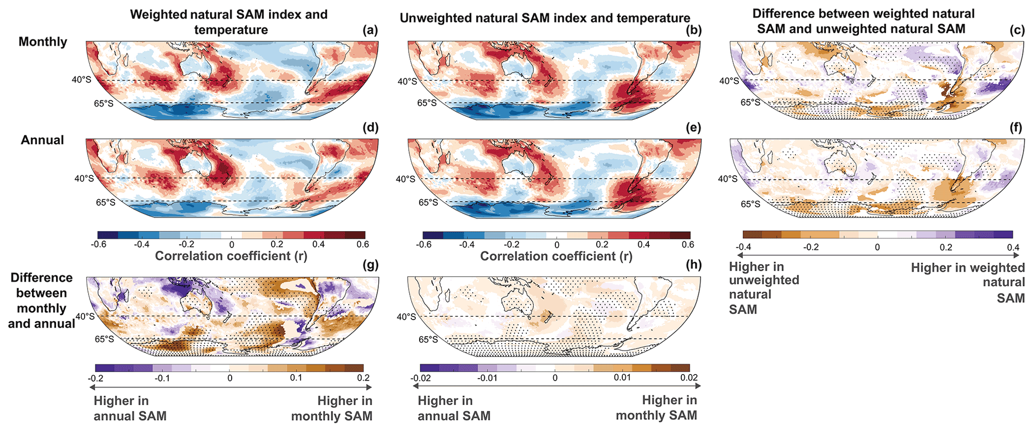
Figure A5 Spatial correlation of annual SAM values with ERA5 2 m air temperature in the Southern Hemisphere (January–December averages over 1950–2022). Comparisons are shown for differences in SAM indices derived from monthly (a, b) and annual (d, e) MSLP data and for latitudinally weighted natural SAM indices (a, d) and unweighted natural SAM indices (b, e; as in Fig. 5). Also shown are the differences in spatial correlation values based on MSLP data resolution (g, h) and for weighted natural versus unweighted natural SAM indices (c, f). In these correlation difference plots, the shading represents differences between methods and data resolution while stippling indicates regions of negative spatial correlations.

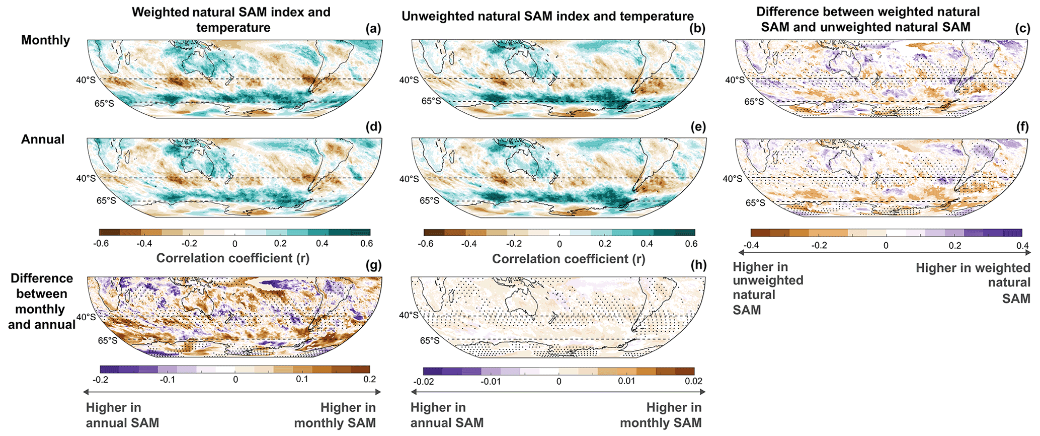
Figure A6 Spatial correlation of annual SAM values with ERA5 precipitation in the Southern Hemisphere (January–December averages over 1950–2022). Comparisons are shown for differences in SAM indices derived from monthly (a, b) and annual (d, e) MSLP data and for latitudinally weighted natural SAM indices (a, d) and unweighted natural SAM indices (b, e; as in Fig. 6). Also shown are the differences in spatial correlation values based on MSLP data resolution (g, h) and for weighted natural versus unweighted natural SAM indices (c, f). In these correlation difference plots, the shading represents differences between methods and data resolution while stippling indicates regions of negative spatial correlations.