the Creative Commons Attribution 4.0 License.
the Creative Commons Attribution 4.0 License.
 | 02 May 2024
Highly stratified mid-Pliocene Southern Ocean in PlioMIP2
Julia E. Weiffenbach
Henk A. Dijkstra
Anna S. von der Heydt
Ayako Abe-Ouchi
Wing-Le Chan
Deepak Chandan
Ran Feng
Alan M. Haywood
Stephen J. Hunter
Xiangyu Li
Bette L. Otto-Bliesner
W. Richard Peltier
Christian Stepanek
Ning Tan
Julia C. Tindall
Zhongshi Zhang
During the mid-Pliocene warm period (mPWP; 3.264–3.025 Ma), atmospheric CO2 concentrations were approximately 400 ppm, and the Antarctic Ice Sheet was substantially reduced compared to today. Antarctica is surrounded by the Southern Ocean, which plays a crucial role in the global oceanic circulation and climate regulation. Using results from the Pliocene Model Intercomparison Project (PlioMIP2), we investigate Southern Ocean conditions during the mPWP with respect to the pre-industrial period. We find that the mean sea surface temperature (SST) warming in the Southern Ocean is 2.8 °C, while global mean SST warming is 2.4 °C. The enhanced warming is strongly tied to a dramatic decrease in sea ice cover over the mPWP Southern Ocean. We also see a freshening of the ocean (sub)surface, driven by an increase in precipitation over the Southern Ocean and Antarctica. The warmer and fresher surface leads to a highly stratified Southern Ocean that can be related to weakening of the deep abyssal overturning circulation. Sensitivity simulations show that the decrease in sea ice cover and enhanced warming is largely a consequence of the reduction in the Antarctic Ice Sheet. In addition, the mPWP geographic boundary conditions are responsible for approximately half of the increase in mPWP SST warming, sea ice loss, precipitation, and stratification increase over the Southern Ocean. From these results, we conclude that a strongly reduced Antarctic Ice Sheet during the mPWP has a substantial influence on the state of the Southern Ocean and exacerbates the changes that are induced by a higher CO2 concentration alone. This is relevant for the long-term future of the Southern Ocean, as we expect melting of the western Antarctic Ice Sheet in the future, an effect that is not currently taken into account in future projections by Coupled Model Intercomparison Project (CMIP) ensembles.
- Article
(7491 KB) - Full-text XML
-
Supplement
(16497 KB) - BibTeX
- EndNote


The Southern Ocean is a critical component of the Earth's climate system, as it acts as a major sink of heat and carbon dioxide (Khatiwala et al., 2009; Tjiputra et al., 2010; Iudicone et al., 2011) and affects global ocean circulation patterns (Talley, 2013; Rintoul, 2018). Close to the Antarctic margin, dense Antarctic Bottom Water (AABW) is formed that fills the abyssal ocean of the Atlantic and Indo-Pacific basins (Orsi et al., 1999; Johnson, 2008). Further north, strong westerly winds drive the upwelling of Circumpolar Deep Water (Marshall and Speer, 2012) and downwelling of Antarctic Intermediate Water (Sloyan and Rintoul, 2001). The Southern Ocean circulation plays a vital role in mitigating the current rise in atmospheric CO2 levels through its uptake of CO2, where it is estimated that over 1999–2007 the Southern Ocean has taken up 40 % of excess anthropogenic carbon present in seawater (Bopp et al., 2015). In addition, through its heat uptake, the Southern Ocean modulates rising global air temperatures and ocean heat content (Frölicher et al., 2015; Liu et al., 2018).
While there have been several model studies concerning the impact of rising CO2 levels on the future Southern Ocean (e.g., Ito et al., 2015; Bracegirdle et al., 2020; Almeida et al., 2021), these studies consider transient simulations following Coupled Model Intercomparison Project (CMIP) scenarios. Due to the absence of slow feedbacks, they cannot not inform us of the long-term impacts of higher CO2 levels on the global and regional climate and typically do not take into account Antarctic Ice Sheet adjustment in a warming climate. One way to consider these effects is by studying warm paleoclimates during geological periods in which the atmospheric CO2 concentration was similar to that of a possible near-future warm climate. One of these periods is the mid-Pliocene warm period (mPWP; 3.264–3.025 Ma). Burke et al. (2018) have shown that the near-future climate stabilized at the Representative Concentration Pathway 4.5 (RCP4.5) scenario is similar to the climate during the mPWP, and this period can therefore be considered a good geological analog for long-term future climate under moderate CO2 emissions. The mPWP is the most recent geological period during which the CO2 concentration was around 400 ppm (e.g., Seki et al., 2010; Pagani et al., 2010; de la Vega et al., 2020), which is close to present-day levels. The mPWP global mean surface temperature was ∼3 °C higher than during the pre-industrial (PI) (Haywood et al., 2013, 2020; McClymont et al., 2020a). Geographic boundary conditions were also similar to present-day conditions, with some important differences including a substantially reduced Greenland Ice Sheet (Dolan et al., 2015), absence of the West Antarctic Ice Sheet, reduction in the East Antarctic Ice Sheet (Dowsett et al., 2010), and a different configuration of mostly high-latitude Northern Hemisphere (NH) ocean gateways, including the Bering Strait and Canadian Archipelago (Dowsett et al., 2016).
The Pliocene Model Intercomparison Project Phase 2 (PlioMIP2) encompasses an ensemble of 17 Earth system models and was initiated to investigate the mPWP climate and to study its potential as a future climate analog (Haywood et al., 2016). Each participating model has provided at least a mPWP simulation (Eoi400) and a PI simulation (E280). The mPWP Eoi400 simulations are centered on an interglacial peak, the KM5c time slice at 3.205 Ma, during which orbital forcing was similar to present day. The mPWP boundary conditions, including orography, ice sheet extent, and vegetation cover, are prescribed based on the reconstruction by the Pliocene Research, Interpretation and Synoptic Mapping (PRISM4) project (Dowsett et al., 2016). Previous studies using the PlioMIP2 ensemble have shown that surface temperature proxies generally agree well with the models (Haywood et al., 2020; McClymont et al., 2020a) but that the boundary conditions, including orography, vegetation, and ice sheet conditions, can have a strong regional influence on the simulated mPWP climate (Feng et al., 2022; Burton et al., 2023).
While the influence of orographic changes on the simulated mPWP climate can reduce the suitability of the mid-Pliocene warm period as a geological analog for a future climate, the smaller ice sheet cover over Antarctica and Greenland during the mPWP can be very relevant for informing us on the impact of higher CO2 levels combined with reduced ice sheet cover in the long-term future. In the Southern Hemisphere (SH) polar region, there are few orographic differences between the Eoi400 and E280 cases, apart from those related to the reduced Antarctic Ice Sheet (Dowsett et al., 2016). It is therefore likely that the Southern Ocean in the mPWP simulations is primarily affected by a higher CO2 level and the reduced Antarctic Ice Sheet cover. While the reconstructed ∼24 m sea level equivalent of combined ice mass loss from the Greenland Ice Sheet and Antarctic Ice Sheet in the mPWP (Haywood et al., 2016) seems unlikely for near-future scenarios, future projections on multi-centennial timescales do show substantial Antarctic Ice Sheet loss and potential West Antarctic Ice Sheet collapse under multiple climate scenarios (Cornford et al., 2015; Golledge et al., 2015; DeConto and Pollard, 2016; Bulthuis et al., 2019; Pattyn and Morlighem, 2020). Studying the state of the Southern Ocean in the mPWP simulations can therefore provide valuable insight into the impact of a reduced Antarctic Ice Sheet on both global and Southern Hemisphere ocean conditions in a warm equilibrium climate.
In this study, we will use model output from the PlioMIP2 ensemble to investigate Southern Ocean conditions during the mPWP. Our aim is to answer the following questions:
-
What are the differences between mPWP and PI states of the Southern Ocean, and how do these impact the abyssal global ocean circulation?
-
How much do mPWP boundary conditions, primarily the reduced Antarctic Ice Sheet, contribute to the difference in Southern Ocean conditions between the mPWP and the PI, and what are the resulting implications for a possible future climate?
To answer the first question, we will look at changes in Southern Ocean conditions in the mPWP compared to the PI in the PlioMIP2 models. This analysis includes sea ice extent, temperature, and salinity changes in the ocean, as well as atmospheric variables such as precipitation and wind that are first-order controls on the oceanography of the Southern Ocean. We will then link changes in these variables to altered deep-ocean circulation and ocean heat and freshwater transport in the Southern Ocean. For the second question, we consider seven additional E400 sensitivity simulations of the ensemble. These simulations are in equilibrium at a mid-Pliocene CO2 level, 400 ppm, but do not feature mPWP boundary condition changes. Using these sensitivity simulations, we assess to what extent sea ice, temperature, and salinity changes are influenced by a reduced Antarctic Ice Sheet.
2.1 PlioMIP2 experimental design
The participating models of PlioMIP2 performed two core simulations (Haywood et al., 2016). Each model performed a PI control simulation (E280) at approximately 280 ppm CO2 and a mPWP simulation (Eoi400) at 400 ppm CO2, both with a simulation length set to be as long as possible or at least 500 model years. The mPWP Eoi400 simulation is performed using the PRISM4 boundary conditions (Dowsett et al., 2016). These boundary conditions prescribe a mPWP land–sea mask, topography, bathymetry, vegetation, soils, lakes, and land ice cover. These boundary conditions include the closure of the Bering Strait and Canadian Archipelago in the mPWP, as well as modifications to other seaways. The Greenland Ice Sheet was substantially reduced to approximately 25 % of its modern-day cover, where land ice remains only in the eastern Greenland mountains. The Antarctic Ice Sheet prescribed by PRISM4 has no ice over western Antarctica and reduced ice cover over eastern Antarctica. The total reduction in the global ice sheet volume is equivalent to a sea level increase less than ∼24 m with respect to the present day (Dowsett et al., 2016). Trace gases, orbital parameters, and the solar constant in the mPWP Eoi400 simulation are set to the same value as the model's PI E280 simulation. For the full details of the experimental design of PlioMIP2, the reader is referred to Haywood et al. (2016).
2.2 Data
We use datasets from simulations performed with 15 out of 17 models participating in PlioMIP2. NorESM-L and MRI-CGCM2.3 are excluded from this study because not all necessary data are available. Table 1 lists the 15 models used in this study, along with their resolution and reference. It is important to note that 5 out of the 15 models in the ensemble are Community Earth System Models (CESMs), of which 3 are CCSM4 models, creating an imbalance in the ensemble. However, due to differences in model versions, as well as model settings of individual groups, earlier PlioMIP2 studies show that the climate response varies significantly among the CESM members (e.g., Haywood et al., 2020; Z. Zhang et al., 2021), and we therefore consider it unlikely that this imbalance skews our results.
Feng et al. (2020)Peltier and Vettoretti (2014)Chandan and Peltier (2017)Baatsen et al. (2022)Feng et al. (2020)Feng et al. (2020)Feng et al. (2022)Stepanek et al. (2020)Q. Zhang et al. (2021)Hunter et al. (2019)Williams et al. (2021)Tan et al. (2020)Tan et al. (2020)Lurton et al. (2020)Chan and Abe-Ouchi (2020)Li et al. (2020)Table 1Overview of PlioMIP2 models used in this study. E400 sensitivity experiments have been provided by models typeset in bold.

* Pre-industrial land–sea mask in both simulations.
Each of the models listed in Table 1 has completed the PI E280 simulation and the mPWP Eoi400 simulation with the mPWP boundary conditions that are described in Haywood et al. (2016). All models that are analyzed in this study, except HadGEM3, use the mPWP boundary conditions that include changes to the land–sea mask and ocean bathymetry. HadGEM3 uses a pre-industrial land–sea mask in both simulations. Additionally, seven model groups have performed a sensitivity study in which a PI simulation is performed at 400 ppm CO2 (E400). We use this simulation to separate the effect of increased CO2 levels from that of other mPWP boundary conditions.
2.3 Analysis
We have used 100-year averages for all PlioMIP2 model fields, except for IPSL-CM5A and IPSL-CM5A2. For the latter two models, we have used the available 50-year averages for E280 and Eoi400 experiments and a 30-year average for the E400 IPSL-CM5A2 experiment. Ocean freshwater and heat transport have been calculated on native model grids, except for COSMOS, where computation is done on a regular interpolated 1×1° grid, as the native curvilinear grid is unsuitable for this calculation. All other variables are horizontally interpolated to a regular 1×1° grid, and any spatial averages presented in this study are calculated from these fields. Unless indicated otherwise, an anomaly is defined as Eoi400–E280, and any percentage anomalies are defined with respect to E280.
The multi-model mean (MMM) is calculated by averaging over all the models in Table 1. The special model mean (SMM) is calculated by averaging over the seven models that have E400 data. In Fig. S1 in the Supplement, we compare the E280, Eoi400, and Eoi400–E280 SMM and MMM of surface variables used in this study. For the Southern Ocean, the SMM–MMM difference in the spatially averaged Eoi400–E280 sea surface temperature (SST) anomaly is approximately −0.5 °C. The models included in the SMM therefore show substantially colder Southern Ocean SSTs than those included in the MMM. The difference in average sea surface salinity (SSS) anomaly is less than 0.1 psu. The location of the MMM and SMM sea ice edge (15 % sea ice cover) is almost identical, although there are local differences in sea ice cover between the SMM and MMM.
The stratification of the Southern Ocean is analyzed using the potential density ρ, which is calculated from potential temperature and salinity fields using the TEOS-10 equation of state (Roquet et al., 2015). To provide a measure for the stratification, we use the following stratification index (SI), following Bourgeois et al. (2022), based on Sgubin et al. (2017):
where z0 is the sea surface and for i=1, …, 10 (units in m).
Averages for the Southern Ocean are calculated over all grid cells between 45–90° S, unless indicated otherwise. We calculate the Antarctic sea ice area as the sum of the product of the sea ice cover fraction and the grid cell area over all SH ocean grid cells. For Eoi400, only grid cells that were also ocean grid cells in E280 were included in this analysis. Thus, any additional sea ice that is formed in the mPWP in areas where the land–sea mask has changed from land to sea is not taken into account. This is to avoid bias in the sea ice area anomaly due to ocean cells being created in locations where the Antarctic Ice Sheet has disappeared.
Furthermore, we use the following definitions for the Atlantic Meridional Overturning Circulation (AMOC) and the abyssal deep-cell circulation: the AMOC strength is the maximum value of the Atlantic meridional overturning streamfunction at latitudes north of 0° N and below a depth of 500 m, and the abyssal deep-cell circulation strength is the absolute value of the most negative global meridional overturning streamfunction below a depth of 1000 m.
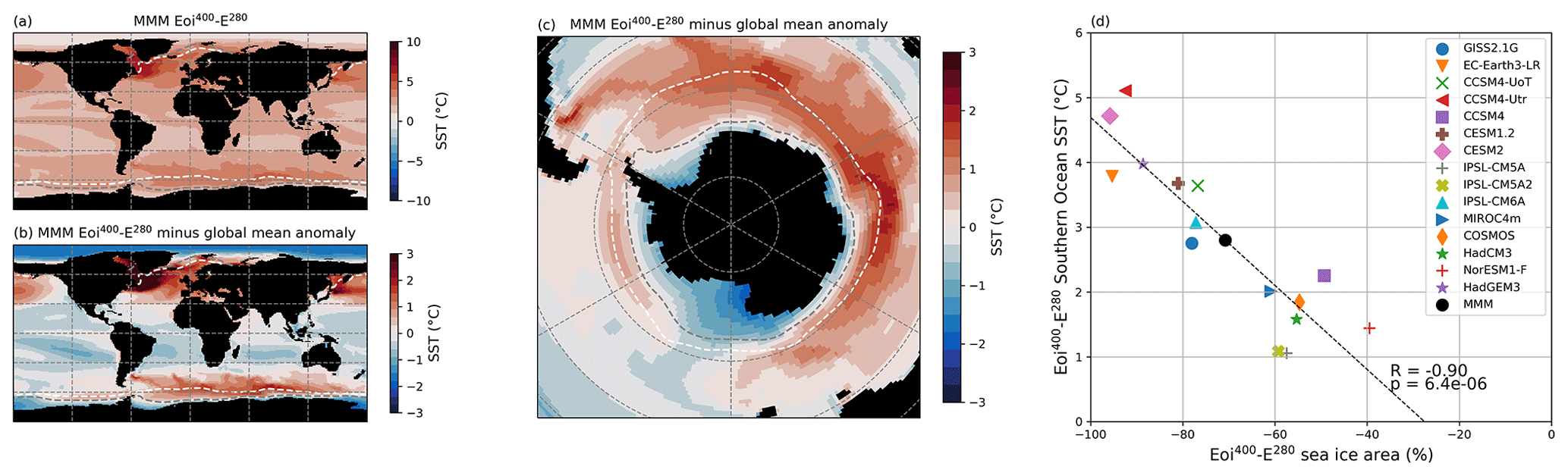
Figure 1(a) Multi-model mean (MMM) Eoi400–E280 sea surface temperature (SST) anomaly. (b) MMM Eoi400–E280 SST anomaly minus the MMM global mean SST anomaly. (c) Same as panel (b) but on an orthographic projection centered on Antarctica. Dashed white and gray lines show the MMM annual mean sea ice edge (15 % sea ice cover) in E280 and Eoi400, respectively. (d) Scatterplot of the individual model sea ice area anomaly relative to E280 versus the SST anomaly in the Southern Ocean (45–90° S). Dashed line shows a linear least squares fit, with the indicated correlation (R value) and p value. E280 and Eoi400 are the respective PI and mPWP experiments.
2.4 Results
2.4.1 Mid-Pliocene Southern Ocean in PlioMIP2
Figure 1a shows the MMM Eoi400-E280 SST anomaly. The MMM global average SST is 2.4 °C warmer in the mPWP than in the PI, while the Southern Ocean (45–90° S) is 2.8 °C warmer. The ratio of SST warming in the Southern Ocean to global average warming, the Southern Ocean SST amplification, is therefore 1.2. We can see regions of amplified warming more clearly in Fig. 1b, which shows the MMM SST anomaly minus the MMM global average SST anomaly. Warming amplification occurs in both the Northern Hemisphere and Southern Hemisphere at latitudes higher than approximately 40° in regions where sea ice cover is absent in the Eoi400 simulations.
From Fig. 1c, which focuses on the southern polar region, it is clear that the largest SST warming amplification in the Eoi400 simulations occurs around the pre-industrial sea ice edge. In locations where sea ice cover persists in the mPWP, the warming is at or below the global average. There is a strong correlation between the Southern Ocean temperature anomaly and sea ice area decrease within the models ( and p<0.05; Fig. 1d). Models with a relatively large decrease in sea ice area generally also experience the highest SST warming in the Southern Ocean. Sea ice reduction is therefore correlated to mPWP polar amplification in the Southern Hemisphere, although the analysis performed does not exclude the possibility that other mechanisms may be at work. Across the study ensemble, the MMM decrease in sea ice area in the mPWP is 71 % with respect to the pre-industrial sea ice area.
Burton et al. (2023) show that higher mPWP CO2 levels combined with the reduced albedo of the SH polar region are the main drivers behind the warming in this region. The 60—90° S average annual mean MMM SAT is 7.6 °C higher than in the PI. When normalized by the MMM global average SAT warming of 3.4 °C, we find a SH polar amplification index of 2.2. This is substantially higher than both the CMIP6 abrupt-4 × CO2 SH polar amplification of 1.1 (centered around year 100) and the CMIP6 historical (1979–2014) SH polar amplification of 0.9 (Hahn et al., 2021), in which simulations are purely driven by fast feedbacks and ice sheet adjustments are not taken into account (Eyring et al., 2016). The amplified SAT warming over the majority of Antarctica and the high-latitude Southern Ocean (Fig. S2) likely contributes to the increase in precipitation over many parts of the SH polar region in the mPWP with respect to the PI (Fig. 2a). The MMM increase in precipitation over the Southern Ocean and Antarctica is 0.35 mm d−1 (+14 %) and 0.36 mm d−1 (+50 %), respectively. Part of this increase in precipitation, particularly over the Southern Ocean, is offset by an equal or even larger increase in evaporation, as illustrated by the net surface freshwater flux anomaly in Fig. 2b. Nevertheless, the net change in surface freshwater flux is still positive over the majority of the Southern Ocean, with a MMM increase in surface freshwater flux of 0.13 mm d−1 (+10 %). We find that, as a result, the majority of the Southern Ocean becomes less saline at the surface, especially close to the Antarctic continent and that this salinity decrease is robust across the PlioMIP2 ensemble (Fig. 2c). The MMM change in Southern Ocean sea surface salinity (SSS) is −0.17 psu, with local minima down to −3.0 psu.
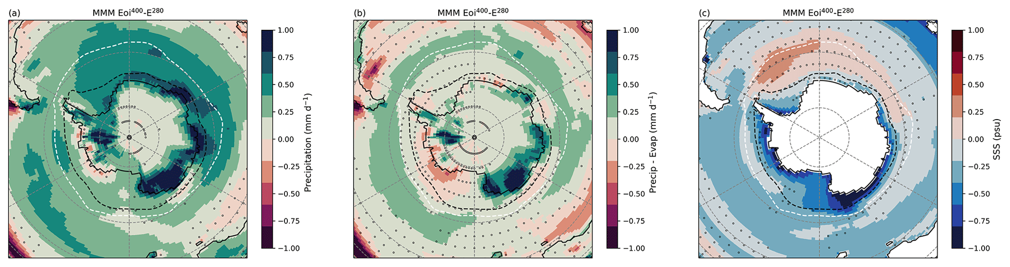
Figure 2(a) Multi-model mean (MMM) Eoi400–E280 precipitation anomaly. (b) MMM Eoi400–E280 surface freshwater flux (precipitation minus evaporation) anomaly. (c) MMM Eoi400–E280 sea surface salinity (SSS) anomaly. Stippling indicates that fewer than 12 out of 15 (<80 %) models agree on the sign of change. Dashed white and black lines show the MMM annual mean sea ice edge (15 % sea ice cover) in E280 and Eoi400, respectively. E280 and Eoi400 are the respective PI and mPWP experiments.
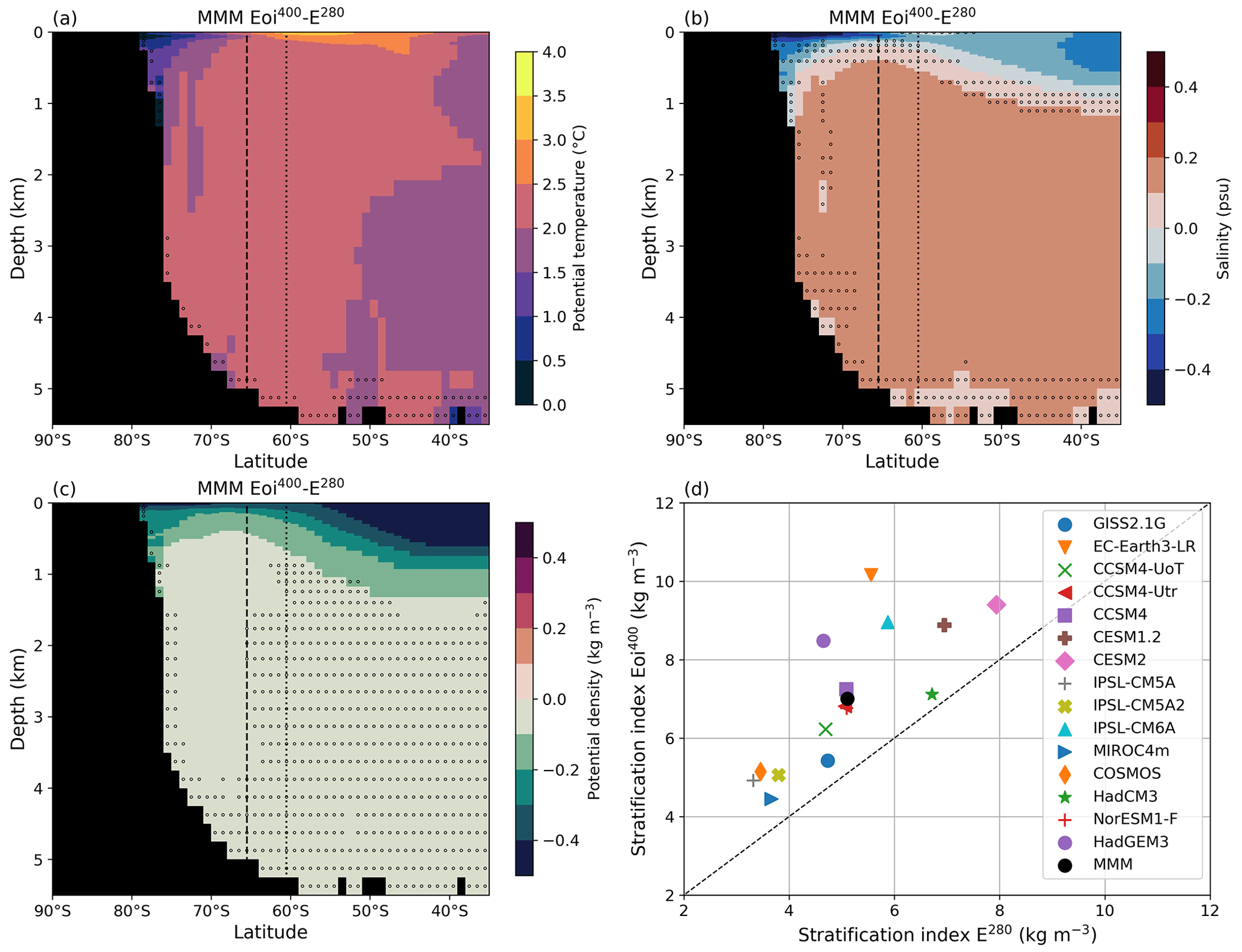
Figure 3(a) Multi-model mean (MMM) zonal mean Eoi400–E280 potential temperature anomaly. (b) MMM zonal mean Eoi400–E280 salinity anomaly. (c) MMM zonal mean Eoi400–E280 potential density anomaly. Stippling indicates that fewer than 12 out of 15 (<80 %) models agree on the sign of change. Vertical dotted and dashed lines indicate the MMM annual mean zonal mean sea ice edge (15 % sea ice cover) in E280 and Eoi400, respectively. (d) Scatterplot of the high-latitude (>60° S) Southern Ocean stratification index in E280 PI and mPWP experiments. E280 and Eoi400 are the respective PI and mPWP experiments.
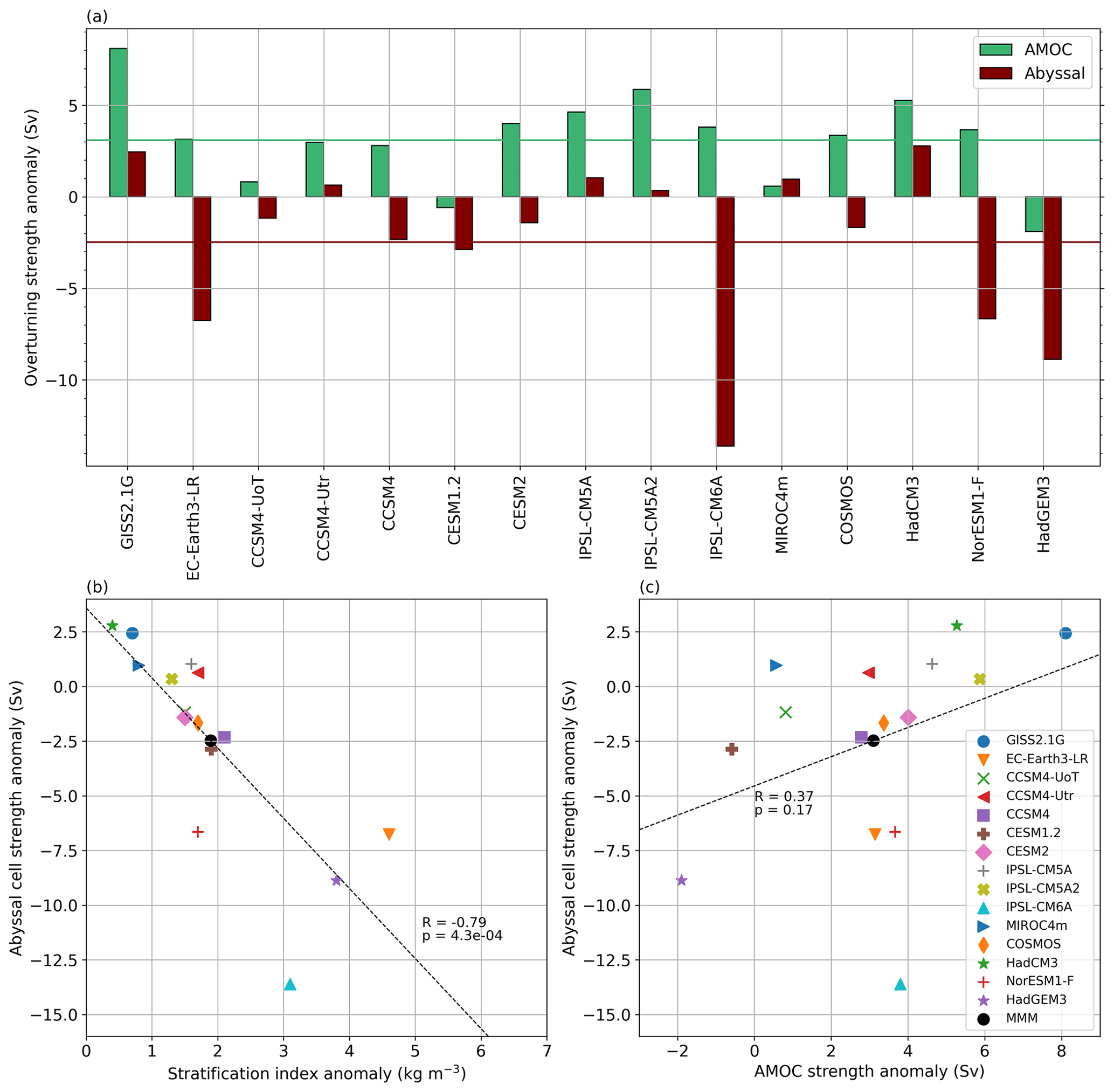
Figure 4(a) Individual model Eoi400–E280 Atlantic Meridional Overturning Circulation (AMOC) and abyssal overturning strength anomalies. Horizontal lines indicate the multi-model mean (MMM) overturning strength anomalies. (b) Scatterplot of individual model Eoi400–E280 Southern Ocean stratification index anomalies against the abyssal cell strength anomalies. (c) Scatterplot of individual model Eoi400–E280 AMOC strength anomalies against the abyssal cell strength anomalies. Dashed lines show a linear least squares fit to the individual model data, with indicated correlation (R) and p values. E280 and Eoi400 are the respective PI and mPWP experiments.
As Figs. 1 and 2 show, the majority of the surface of the Southern Ocean both freshens and warms in the Eoi400 simulations with respect to E280. It is inevitable that these changes affect the density stratification in the Southern Ocean. Figure 3a and b show the MMM Southern Ocean zonal mean potential temperature and salinity anomalies, respectively. The warming is quite uniform throughout the water column, apart from relatively low surface warming close to Antarctica and an increase in surface warming between approximately 45–65° S. In contrast, in the MMM zonal mean salinity anomaly, we see a clear pattern emerging that features a fresher ocean surface and saltier deeper ocean across all latitudes in the mid-Pliocene Southern Ocean. The same pattern is reflected in the MMM zonal mean potential density anomaly in Fig. 3c. In most models, we see a stronger stratification in the mid-Pliocene Southern Ocean than in the pre-industrial (Fig. S3). At high latitudes (>60° S), the increase in stratification is consistent across all PlioMIP2 ensemble members, as illustrated by their increase in high-latitude Southern Ocean stratification index (Fig. 3d; Table S1 in the Supplement). The high-latitude Southern Ocean stratification index is defined as the average stratification index over all latitudes higher than 60° S, which is where abyssal deep-water formation takes place. The gridded individual model stratification index anomalies are shown in Fig. S4. The MMM Eoi400–E280 high-latitude Southern Ocean stratification index anomaly is 1.9 kg m−3, corresponding to a relative increase of 37 % with respect to the E280 MMM.
AABW formation is driven by buoyancy loss at the ocean surface. Consequently, the substantial increase in density stratification in high-latitude, non-circumpolar waters of the Southern Ocean is likely to have an impact on abyssal ocean circulation. Figure 4a shows the individual model and MMM Eoi400–E280 anomalies of the AMOC and abyssal overturning strengths. Overall, we see a decrease in abyssal cell strength in 9 out of 15 models, with a MMM decrease of 2.5 Sv (−22 %). The MMM AMOC strength increases by 3.1 Sv (+16 %) in the mPWP simulations with respect to the PI, which agrees with Z. Zhang et al. (2021), who show a consistently stronger mPWP AMOC in PlioMIP2. As 13 out of 15 models show a stronger mid-Pliocene AMOC, the response of the AMOC cell is more consistent than that of the abyssal cell.
The abyssal cell circulation strength should be related to the volume of deep-water formation in the Southern Ocean and therefore to surface water buoyancy in the high-latitude Southern Ocean. We find that the high-latitude (>60° S) Southern Ocean stratification index anomaly shows a significant anti-correlation (; p=0.001) with the abyssal cell strength anomaly (Fig. 4b). The increased Southern Ocean stratification in the mid-Pliocene simulations therefore indeed appears to significantly impact the abyssal cell circulation and thereby the global ocean circulation. It is interesting, however, that the six models that do not feature a decrease in the abyssal cell strength still have a more stratified high-latitude Southern Ocean (Fig. 4b). Figure 4c shows that four out of these six models do have the highest AMOC anomaly of the ensemble, which points to a possible interaction between the abyssal cell and the AMOC cell.
When correlating the abyssal cell strength and the AMOC cell strength anomalies, there is no significant correlation (Fig. 4d). However, when the outlier IPSL-CM6A is removed, the correlation does become significant (R=0.57; p=0.03). A possible explanation for this correlation is that when the abyssal waters return to the Southern Ocean, both by diapycnal upwelling to intermediate depths and by transport to the surface along isopycnals (Lumpkin and Speer, 2007), they interact with North Atlantic Deep Water (NADW) from the AMOC cell. In the Southern Ocean, wind-driven Ekman transport upwells NADW to the surface to ultimately return northward (Toggweiler and Samuels, 1995), but the majority of NADW is transformed to AABW (Talley, 2013; Rousselet et al., 2021). The stronger AMOC in the Eoi400 simulations is driven by more vigorous NADW formation due to increased salinity in the high-latitude North Atlantic (Weiffenbach et al., 2023). In this way, the higher volume of relatively saline NADW results in more AABW transformation, thereby partly compensating the effects of higher density stratification in the high-latitude Southern Ocean.
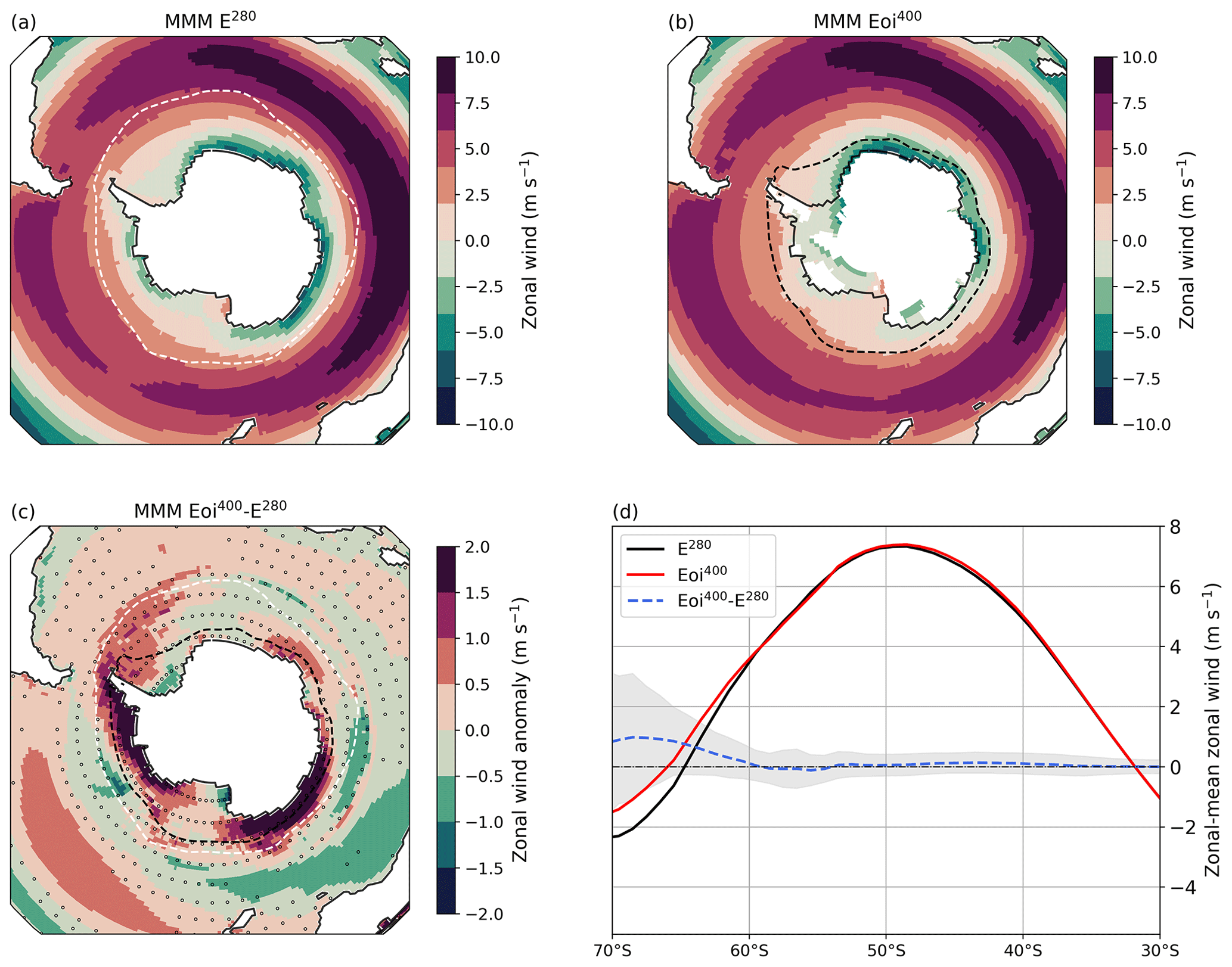
Figure 5(a) Multi-model mean (MMM) E280 1000 hPa zonal wind, where positive values indicate eastward wind. (b) MMM Eoi400 1000 hPa zonal wind. (c) MMM Eoi400–E280 1000 hPa zonal wind anomaly. Stippling indicates that fewer than 12 out of 15 (<80 %) models agree on the sign of change. Dashed white and black lines show the MMM annual mean sea ice edge (15 % sea ice cover) in E280 and Eoi400, respectively. (d) MMM zonal mean 1000 hPa zonal wind in Eoi400, E280, and Eoi400–E280. Shading indicates 1 standard deviation around the MMM Eoi400–E280 anomaly. E280 and Eoi400 are the respective PI and mPWP experiments.
The pattern and strength of the zonal wind stress at the Southern Ocean surface also exert a strong effect on the global meridional overturning circulation through the wind-driven equatorward Ekman transport. Over the past few decades, the westerly winds over the mid-latitude Southern Ocean have been strengthening and shifting polewards (Swart and Fyfe, 2012; Deng et al., 2022). An increase in strength and poleward shift in the mid-latitude Southern Hemisphere westerlies has also been shown under future warming scenarios (e.g., Kidston and Gerber, 2010; Bracegirdle et al., 2013). In PlioMIP2, we do not see any systematic changes in surface westerly winds over the Southern Ocean (Fig. 5). Fewer than half of the models show a poleward shift in the zonal mean surface wind, with a minimal increase in maximum strength (Fig. S5), and there is little agreement over the sign of change, apart from a decrease in westerly wind strength south of Australia and increase in strength over the Pacific sector (Fig. 5c).
The Southern Ocean is the only location where the meridional ocean heat transport (OHT) in the mid-Pliocene simulations differs significantly from the pre-industrial (Fig. 6a; see Fig. S6 for individual model plots). Between 35–65° S, the MMM poleward heat transport reduces by 0.040 PW (−19 %). We show in Fig. 6b that the decrease in Southern Ocean ocean heat transport is significantly correlated with the decrease in abyssal cell strength (; p=0.002). The four models that show an increase in poleward OHT in the Southern Ocean feature a stronger rather than weaker abyssal cell. This is consistent with Menviel et al. (2015), who show that a stronger AABW circulation leads to an increase in poleward heat transport. These results suggest that mid-Pliocene changes in abyssal cell strength affect the Southern Ocean heat transport.
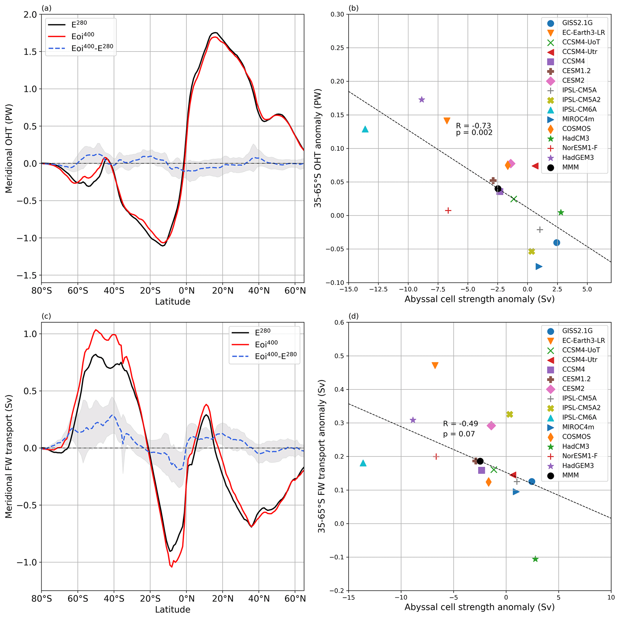
Figure 6(a) Multi-model mean (MMM) meridional ocean heat transport (OHT) in Eoi400, E280, and Eoi400–E280; positive values indicate northward transport. Shading indicates 1 standard deviation around the MMM Eoi400–E280 anomaly. (b) Scatterplot of the individual model Eoi400–E280 abyssal cell strength anomaly against the 35–65° S average OHT anomaly. Dashed lines show a linear least squares fit to the individual model data, with indicated correlation (R) and p values. (c, d) Same as panels (a) and (b) for the northward meridional freshwater transport (FWT), respectively. E280 and Eoi400 are the respective PI and mPWP experiments.
In the Eoi400 simulations, we also find a significant increase in northward freshwater transport in the Southern Ocean with respect to the E280 (Fig. 6c; see Fig. S7 for individual model plots). The northward freshwater transport increases between 35–65° S by 0.19 Sv (+31 %). Figure 6d shows a correlation between the Southern Ocean freshwater transport anomaly and the abyssal cell strength that is just outside the 95 % significance interval (; p=0.07). The weakest increase or even decrease in northward freshwater transport is again shown by a subset of models that does not have a weaker abyssal cell circulation in the mid-Pliocene. It is also important to consider that the OHT and freshwater transport anomalies will likely be influenced by the stronger AMOC in the mid-Pliocene simulations. We do not, however, find a significant correlation between Southern Ocean heat or freshwater transport and the AMOC strength (Fig. S8).
2.4.2 Influence of boundary conditions and CO2
The results in the previous section indicate that the density stratification of the mid-Pliocene Southern Ocean increases with respect to the pre-industrial in the PlioMIP2 ensemble, illustrating a significant impact on the global abyssal cell overturning circulation and its associated heat and freshwater transport. It is imperative to further investigate the cause of the changes in temperature and salinity in the Southern Ocean that is driving increased density stratification in the mPWP. To this end, we employ the seven available E400 sensitivity simulations to separate the effects of CO2 concentration and geographic boundary conditions, in particular the reduction in the Antarctic Ice Sheet in the Eoi400 simulations. In this section, for all the comparisons between Eoi400, E400, and E280 cases, we use the SMM, i.e., the mean of the seven models that have an E400 simulation.
Figure 7a–c illustrate that the effect of the mid-Pliocene boundary conditions on the sea ice area is substantial. Where an increase in CO2 from 280 to 400 ppm causes a decrease in sea ice area of 28 % relative to the pre-industrial, implementing mid-Pliocene boundary conditions causes an additional 31 % of sea ice area loss. Figure 7d–f reinforce the earlier link that we found between enhanced warming in the Southern Ocean and sea ice area decrease (in which we do not find an amplification of Southern Ocean warming in E400). The SMM Southern Ocean SST amplification is 0.9 in E400, while the SMM Southern Ocean amplification index is 1.1 in Eoi400, which is 0.1 lower than the MMM Eoi400 Southern Ocean amplification index. The Southern Ocean SST amplification observed in Eoi400 simulations is therefore mainly a consequence of the mPWP geographic boundary conditions. The SMM Southern Ocean average E400–E280 SST anomaly is 1.1 °C, while the Eoi400–E280 anomaly is 2.3 °C. This means that the CO2 forcing and mPWP boundary conditions both contribute approximately equally to mPWP Southern Ocean warming.

Figure 7(a) Special model mean (SMM; see Sect. 2) E280 annual mean sea ice cover. Dashed white line indicates the SMM annual mean sea ice edge (15 % sea ice cover). (b, c) Same as panel (a) for E400 and Eoi400. (d) SMM E400–E280 sea surface temperature (SST) anomaly minus the SMM global mean SST anomaly. (e, f) Same as panel (d) for Eoi400–E400 and Eoi400–E280. Dashed white, blue, and black lines show the SMM annual mean sea ice edge (15 % sea ice cover) in E280, E400, and Eoi400, respectively. Note that panel (f) is the same as Fig. 1c, but here the SMM is shown. E280 and Eoi400 are the respective PI and mPWP experiments, and E400 is the PI experiment at 400 ppm CO2.
The SMM precipitation over the Southern Ocean and Antarctica is generally higher in Eoi400 than in E400 with respect to E280 (Fig. 8a–c). Over the 45–90° S Southern Ocean, the average SMM precipitation increases by 0.18 mm d−1 (+7 %) in E400 and 0.31 mm d−1 (+12 %) in Eoi400. The increase in precipitation over Antarctica is 0.10 mm d−1 in E400 (+14 %) and 0.30 mm d−1 (+43 %) in Eoi400. The larger increase in precipitation over the Southern Ocean in Eoi400 results in a larger decrease in SMM sea surface salinity than in E400, even though the mPWP boundary conditions also cause a substantial increase in evaporation over parts of the Southern Ocean and Antarctica (Fig. S9). On average, the sea surface salinity of the Southern Ocean decreases more in Eoi400 (−0.12 psu) than in E400 (−0.09 psu; Fig. 8d–f). This difference is larger in the areas close to the Antarctic continent that are covered by sea ice in Eoi400. In these areas, the sea surface salinity decreases by 0.54 psu in Eoi400 and 0.24 psu in E400.
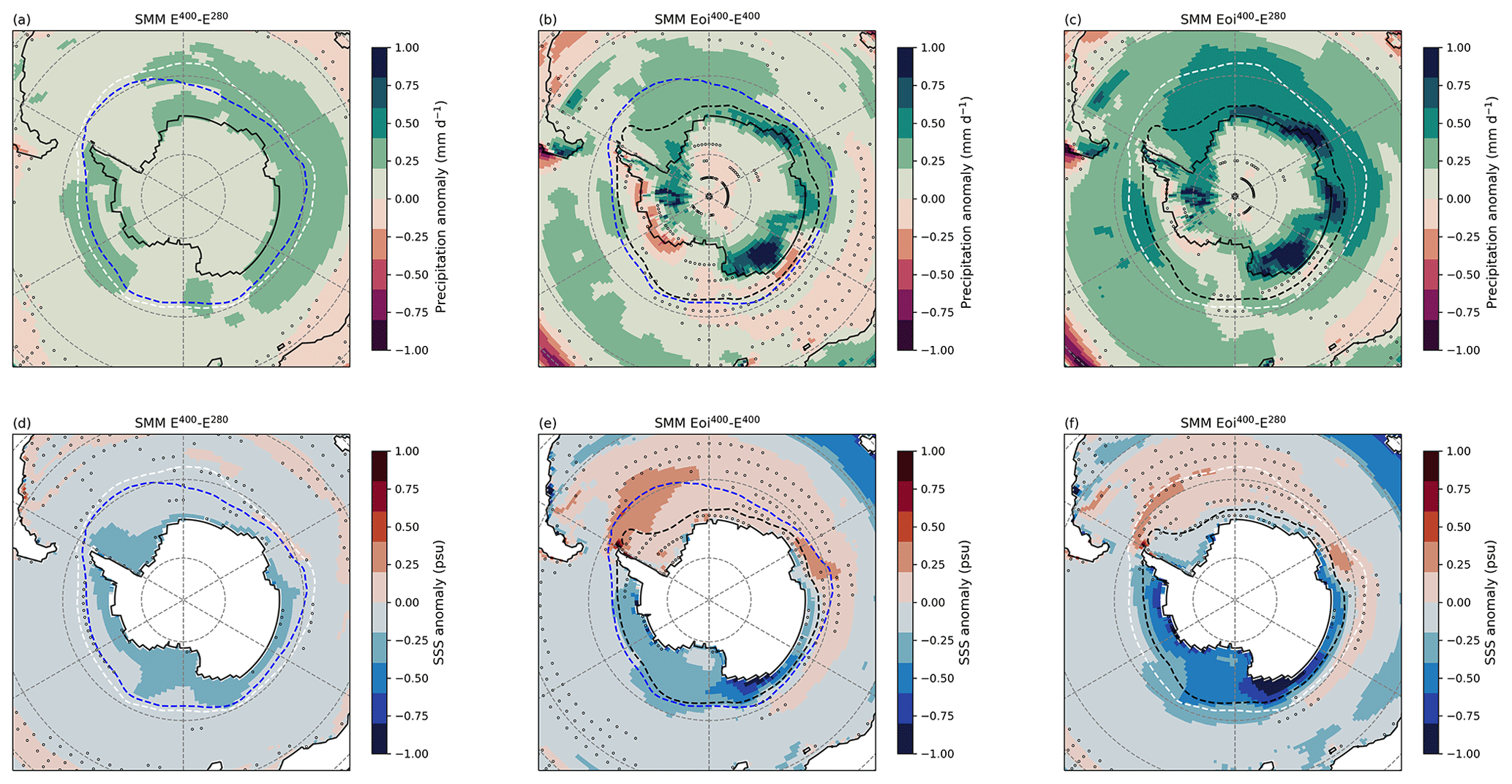
Figure 8(a) Special model mean (SMM; see Sect. 2) E400–E280 precipitation anomaly. (b, c) Same as panel (a) for Eoi400–E400 and Eoi400–E280. Dashed white, blue, and black lines show the SMM annual mean sea ice edge (15 % sea ice cover) in E280, E400, and Eoi400, respectively. Stippling indicates that fewer than five out of seven (<70 %) models included in the SMM agree on the sign of change. (d–f) Same as (a)–(c) but for sea surface salinity (SSS) anomaly. E280 and Eoi400 are the respective PI and mPWP experiments, and E400 is the PI experiment at 400 ppm CO2.
In Fig. 9a–c, we show the SMM zonal mean potential density anomalies in the Southern Ocean. As expected, the warmer and fresher Southern Ocean surface in E400 also results in increased Southern Ocean stratification with respect to E280. The SMM high-latitude (60–90° S) Southern Ocean stratification index increases by 0.7 kg m−3 in E400 (+14 %) and 1.2 kg m−3 (+24 %) in Eoi400 (Table S1). Figure 9e shows that there are substantial regional variations in the SMM E400 and Eoi400 stratification indices. The Eoi400 SMM is less stratified in the Atlantic sector, possibly related to the stronger AMOC, while it is more stratified in the Indo-Pacific sector. At the mid-latitudes, the difference between the SMM 45–60° S average Southern Ocean stratification index anomalies is larger, with 0.8 kg m−3 in E400 (+10 %) and 1.9 kg m−3 (+24 %) in Eoi400. These results suggest that across most of the Southern Ocean, mPWP boundary conditions enhance the increase in Southern Ocean stratification induced by a higher CO2 level.
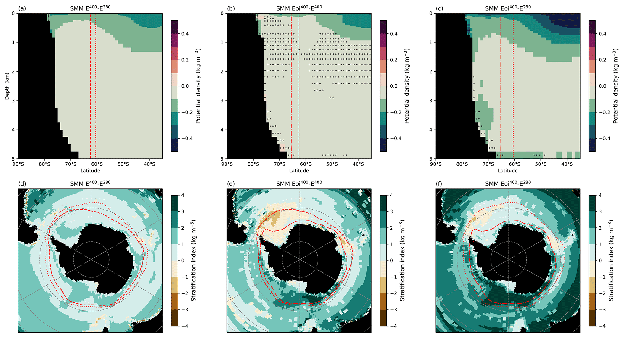
Figure 9(a) Full-depth special model mean (SMM; see Sect. 2) zonal mean E400–E280 potential density anomaly. (b, c) Same as panel (a) for Eoi400–E400 and Eoi400–E280. (d) SMM E400–E280 stratification index anomaly. (e, f) Same as panel (d) for Eoi400–E400 and Eoi400–E280. Stippling indicates that fewer than five out of seven (<70 %) models included in the SMM agree on the sign of change. Dotted, dashed, and dash-dotted red lines show the SMM annual mean sea ice edge (15 % sea ice cover) in E280, E400, and Eoi400, respectively. E280 and Eoi400 are the respective PI and mPWP experiments, and E400 is the PI experiment at 400 ppm CO2.
Despite the greater increase in stratification index in Eoi400 than in E400, the abyssal cell shows a larger and more consistent decrease in the E400 simulations (Fig. 10a). The SMM E400–E280 abyssal cell strength anomaly, −1.9 Sv (−15 %), is nearly double the Eoi400–E280 anomaly of −1.0 Sv (+8 %). There is a significant negative correlation between the stratification index anomaly and the abyssal cell strength anomaly for both E400–E280 and Eoi400–E280, as shown in Fig. 10b. The difference between the slope and y intercept of the E400–E280 and Eoi400–E280 regressions is likely to be related to the interaction of the abyssal circulation with the AMOC. The results suggest that the stronger AMOC in Eoi400 may be partly compensating weakening of the abyssal cell. The AMOC cell is stronger in all Eoi400 simulations with respect to E280 (Fig. 10a), with an SMM increase of 3.4 Sv (+18 %), while the E400 SMM AMOC strength increase of 0.2 (+1 %) is substantially lower, and only three out of seven models simulate a stronger AMOC in E400.

Figure 10(a) Eoi400–E280 and E400–E280 Atlantic Meridional Overturning Circulation (AMOC; green) and abyssal overturning (red) strength anomalies of models included in the special model mean (SMM; see Sect. 2). Horizontal lines indicate the SMM overturning strength anomalies. (b) Scatterplot of SMM ensemble individual model Eoi400–E280 and E400–E280 Southern Ocean stratification index anomalies against the abyssal cell strength anomalies. Dashed black and red lines show a linear least squares fit to the individual model data of the SMM ensemble, with indicated correlation (R) and p values. The multi-model mean (MMM) ensemble Eoi400–E280 regression from Fig. 4b and the Eoi400–E280 anomalies of the models not included in the SMM are shown in light gray. E280 and Eoi400 are the respective PI and mPWP experiments, and E400 is the PI experiment at 400 ppm CO2.
2.5 Discussion
2.5.1 Model–data comparison
There are no data on the Southern Ocean sea ice cover during the KM5c time slice, but there are a number of studies on Pliocene sea ice and ocean temperatures that suggest there was reduced ice cover during this period (e.g., Barron, 1996; Whitehead and Bohaty, 2003; Whitehead et al., 2005; Dowsett et al., 2010). Whitehead et al. (2005) reconstructed winter sea ice cover at Site 1165 (64.380° S, 67.219° E) and Site 1166 (67.696° S, 74.787° E) across the Pliocene. They found a maximum of 78 % less sea ice relative to modern at Site 1165, and a 61 % reduction at Site 1166 during the Pliocene. Our MMM shows a respective relative sea ice concentration decrease of 72 % and 39 % at these locations, respectively, which matches reconstructions reasonably well, considering the range of uncertainty in the reconstructions of at least 30 % (Whitehead et al., 2005).
We also compare Southern Ocean PlioMIP2 SSTs to SST reconstructions from the KM5c time slice. The SST reconstruction by McClymont et al. (2020a) includes six proxy locations in (close proximity to) the Southern Ocean. We compare absolute mPWP SSTs and mPWP–PI SST anomalies at these locations for both the models and data in Fig. S10, using the observed pre-industrial SSTs from the ERSSTv5 1870–1900 dataset (Huang et al., 2017a) and reconstructed mPWP SSTs from McClymont et al. (2020a). While absolute mPWP SST reconstructions generally fall within the range of the PlioMIP2 ensemble SSTs, the average spread of modeled mPWP SSTs is 7.9 °C. This intermodel spread is reduced to 4.1 °C for the mPWP–PI SST anomalies. However, at three out of six SST proxy locations, the reconstructed SST anomaly falls outside the range of the modeled SST anomaly. The models are neither consistently warmer nor colder than the reconstructions, meaning we cannot detect a consistent bias in the modeled or reconstructed Southern Ocean SSTs. The models appear to match absolute mPWP Southern Ocean SSTs reconstructions better than reconstructed mPWP–PI SST anomalies, possibly due to discrepancies between reconstructed and modeled Southern Ocean SSTs in the PI.
2.5.2 Mid-Pliocene Southern Ocean as a future analog
Burton et al. (2023) have shown that the influence of mPWP boundary conditions on the simulated global average mPWP–PI SAT, SST, and precipitation anomalies in PlioMIP2 is substantial. They found that 44 % of the SAT and SST anomaly and 49 % of the precipitation anomaly were driven by non-CO2 forcing. Our results align with this study and show that the mPWP boundary conditions are responsible for approximately half of the average mPWP–PI anomaly in sea ice cover, SST, precipitation, and stratification index in the Southern Ocean. While a separation of effects due to orographic and land ice cover is not possible, it is plausible that this influence is primarily due to the decreased Antarctic Ice Sheet as there are, apart from a closed Indonesian Throughflow, few other changes in SH mPWP boundary conditions with respect to the PI. This may make the mid-Pliocene warm period a good analog for our long-term future climate in which substantial melting of the Antarctic Ice Sheet is expected. We show that mPWP boundary conditions, primarily the reduction in the Antarctic Ice Sheet in the Southern Hemisphere, lead to additional precipitation, sea ice loss, and sea surface warming and are thus responsible for reinforcing increased stratification caused by a rise in CO2 levels. This potential effect of the Antarctic Ice Sheet reduction is not taken into account in the CMIP Earth system model (ESM) projections of future climate but may therefore play an important role in Southern Ocean conditions on multi-centennial timescales. Moreover, a slowly changing ice sheet will contribute to changes in equilibrium climate sensitivity due to state dependence of fast feedback processes (von der Heydt et al., 2016), which is not accounted for in CMIP ESM simulations and multi-century ice sheet projections. It should be taken into account, however, that Antarctic Ice Sheet projections do not show a ∼21 m sea level equivalent decrease in ice volume, which has been reconstructed for the mPWP Antarctic Ice Sheet (Dowsett et al., 2010). Under unabated emission scenarios, multi-centennial projections show a maximum increase in sea level equivalent melt between approximately 5 m (Golledge et al., 2015) and 15 m (DeConto and Pollard, 2016) by 2500 CE, which makes the mPWP ice sheet extent unrealistic, even for longer-term future scenarios. This means that the Southern Ocean conditions from this study are not likely to be analogous to a long-term future, although a partial reduction that includes the collapse of the West Antarctic Ice Sheet would still greatly decrease the ice sheet extent and therefore possibly induce effects similar to those found in this study.
Our results suggest a relationship between increased stratification in the Southern Ocean and a weakened abyssal cell circulation during the mid-Pliocene warm period. CMIP5 studies investigating RCP4.5 and RCP8.5 scenarios show a decline in Antarctic Bottom Water formation due to fresher and warmer Southern Ocean surface conditions and consequentially a slowdown of deep-ocean circulation by the end of the 21st century (Meijers, 2014; Ito et al., 2015). This is consistent with de Lavergne et al. (2014), who show weakening of Southern Ocean deep convection due to surface freshening under the RCP8.5 scenario, as well as recent work by Chen et al. (2023) demonstrating that freshening of the Southern Ocean surface due to Antarctic meltwater induces weakening of deep convection. CMIP6 models also show future Southern Ocean surface warming and sea ice decrease, as well as mixed layer shoaling that suggests the slowdown of AABW formation (Purich and England, 2021).
While the majority of the PlioMIP2 models show a weaker abyssal cell circulation in the mPWP, there are 6 out of 15 ensemble members for which the Southern Ocean stratification increases in the mPWP simulations without showing weakening of the abyssal cell circulation. Interestingly, four of these six models also exhibit the largest AMOC strength increase during the mPWP with respect to the PI. This implies a potential linkage between the AMOC and abyssal cell circulation, where a stronger AMOC during the mid-Pliocene may partially compensate for the reduced formation and circulation of Southern Ocean bottom water. The stronger AMOC in the mPWP PlioMIP2 simulations has been attributed to changes in geographical boundary conditions, specifically the closure of the Bering Strait and Canadian Archipelago (Z. Zhang et al., 2021; Weiffenbach et al., 2023). Since these geographical changes are not relevant for the future, it is uncertain whether the strength of decline in abyssal cell circulation, or the lack of decline exhibited in some models, resembles a plausible future scenario. Given the substantial influence of the intensified AMOC in the mPWP PlioMIP2 simulations on global ocean circulation, it is reasonable to expect that it also impacts Southern Ocean conditions. To disentangle effects of orographic and ice sheet changes, additional sensitivity studies are necessary. Nevertheless, our results highlight the tight interplay between AMOC and abyssal cell, connecting Southern Hemisphere and Northern Hemisphere high latitudes, and their potential to impact fast feedback processes relevant for equilibrium climate sensitivity in various regions of the world.
2.5.3 Southern Ocean biases
From historical CMIP5 and CMIP6 simulations, it is known that low-resolution Earth system models show systematic biases and inaccuracies concerning Southern Ocean surface conditions and deep-ocean circulation. Southern Ocean SSTs are among the most (warm) biased characteristics of Earth system model simulations (e.g., Wang et al., 2022; Zhang et al., 2023)). CMIP5 simulations have been shown to have a consistent warm and low-density bias over the entire water column and show a large spread in the volume and characteristics of Antarctic Bottom Water (Sallée et al., 2013). As most CMIP5 models create deep water by deep convection in the open ocean, which only rarely occurs in reality, bottom water formation processes are not well represented in these low-resolution ESMs (Heuzé et al., 2013). This remains a problem in the newer CMIP6 generation models (Mohrmann et al., 2021). The majority of the PlioMIP2 models are models also used for CMIP5 or CMIP6 and therefore have the same issues representing deep-water formation. As such, changes to deep-cell circulation in the mid-Pliocene warm period may also be biased due to the inaccurate representation of deep-water formation in the Southern Ocean. In addition, it has been shown that the CMIP5 ensemble shows biases in Southern Ocean SSTs due to errors in cloud-related parameterizations (Hyder et al., 2018). These biases have been correlated to simulated Last Glacial Maximum AMOC depth anomalies (Sherriff-Tadano et al., 2023) and could potentially also affect the AMOC and deep-cell circulation in the mPWP.
Another important bias in the PlioMIP2 models concerns the sea ice area. It has been shown that changes in temperature, sea ice area, and precipitation in future projections are strongly tied to the simulated historical mean sea ice area in CMIP5 (Bracegirdle et al., 2015; Kajtar et al., 2021) and the models strongly overestimate the historical variance in the sea ice extent (Zunz et al., 2013). The PlioMIP2 ensemble also features large ranges of uncertainty in sea ice cover, which we have shown to be crucial when it comes to polar amplification and Southern Ocean precipitation. Figure S11 shows that the MMM sea ice cover and extent in the PI E280 simulations is spatially similar to historical observations (1979–2004 NOAA/NSIDC Climate Data Record of Passive Microwave Sea Ice Concentration; Meier et al., 2021), with a MMM E280 sea ice area of 10.4 million km2 and historical observed sea ice area of 9.5 million km2. While the historical observed sea ice area should ideally be compared to historical simulations, Fig. S11 gives some confidence that the simulated MMM E280 sea ice cover is realistic for the PI. However, the sea ice area variation among models is 5.2–15.6 million km2, which is substantially larger than the discrepancy between the MMM E280 and historical observations. Furthermore, the absolute Eoi400–E280 sea ice area anomaly varies between −4.0 and −11.7 million km2, and relative sea ice area anomaly varies between −39 % and −96 %. This large variance in sea ice extent leads to uncertainty about the representativeness of the Southern Ocean conditions in response to both the higher CO2 and the geographic boundary conditions in the mPWP, especially for those models that have a substantially lower or higher sea ice cover than the MMM.
The Southern Ocean simulated by PlioMIP2 is characterized by a large reduction in sea ice area in the mid-Pliocene warm period with respect to the pre-industrial. Due to the increase in CO2 and the Antarctic Ice Sheet reduction, the 60–90° S MMM SAT is 7.6 °C warmer in the mPWP. This results in a polar amplification factor of 2.2 with respect to the global average MMM SAT anomaly of 3.4 °C, which is substantially higher than in future projections. The MMM relative sea ice area decrease is 71 %, with a substantial variation in sea ice area decrease among the 15 models that ranges from −39 % to −96 %. The decrease in Southern Ocean sea ice area is strongly tied to the SST increase in the mPWP, ranging from 1.1 to 5.1 °C, with a MMM increase of 2.8 °C. There is also a robust increase in precipitation, with a MMM increase of 0.35 mm d−1 over the mPWP Southern Ocean and Antarctic continent, resulting in freshening of the ocean surface.
The warm and fresh mPWP Southern Ocean surface leads to an increase in density stratification with respect to the pre-industrial. This is correlated with a slowdown of the global abyssal cell circulation during the mid-Pliocene warm period, affecting both heat and freshwater transport in the Southern Ocean. The CO2 concentration and Antarctic Ice Sheet reduction are primary drivers of warmer and fresher Southern Ocean surface conditions and of deep-ocean circulation in the mid-Pliocene warm period with respect to the pre-industrial. However, we do find a potential interaction of deep abyssal circulation with the stronger AMOC in the mPWP simulations, where the strengthened AMOC partly compensates weakening of the abyssal cell. Increased AMOC strength has been linked to high North Atlantic salinity due to closed Arctic gateways during the mid-Pliocene warm period and therefore does not appear to be directly related to the CO2 increase or Antarctic Ice Sheet reduction.
Sensitivity simulations at the mid-Pliocene CO2 level without any geographic, ice sheet, or vegetation changes also show decreased sea ice area, increased precipitation, and warming and freshening of the ocean surface. This effect is enhanced by mid-Pliocene boundary conditions, in particular by the Antarctic Ice Sheet reduction, where these boundary conditions contribute approximately one-half to the total sea ice area loss, SST warming, precipitation increase, and density stratification increase in the mPWP simulations. This illustrates that it is important to consider the effects of a smaller Antarctic Ice Sheet when projecting for possible long-term future climates. The multi-century reduction in the Antarctic Ice Sheet will drive changes in fast feedback processes (e.g., clouds and sea ice cover) affecting equilibrium climate sensitivity. However, uncertainties are present via the large model spread and biases in sea ice area and Southern Ocean deep-water formation, as well as via the effect of orographic changes on ocean circulation and Southern Ocean conditions. Additional sensitivity studies, where the land–sea mask and ice sheet size are implemented separately, are necessary to be able to separate the effect of orography and ice sheet changes in the mPWP simulations and further investigate the mechanisms behind the mid-Pliocene Southern Ocean's effect on global ocean circulation.
PlioMIP2 data used for this paper are available upon request from Alan M. Haywood (a.m.haywood@leeds.ac.uk), with the exception of IPSL-CM6A, EC-Earth3-LR, and GISS2.1G. PlioMIP2 data from IPSL-CM6A, EC-Earth3-LR, and GISS2.1G can be obtained from the Earth System Grid Federation (ESGF) (https://esgf-node.llnl.gov/search/cmip6/, ESGF, 2023). The U and Mg/Ca SST reconstructions from McClymont et al. (2020a) can be obtained through https://doi.org/10.1594/PANGAEA.911847 (McClymont et al., 2020b). The NOAA/NSIDC Climate Data Record of Passive Microwave Sea Ice Concentration dataset from Meier et al. (2021) can be obtained through https://doi.org/10.7265/efmz-2t65 The observational pre-industrial SSTs from the NOAA ERSST5 dataset (Huang et al., 2017a) can be downloaded from https://doi.org/10.7289/V5T72FNM (Huang et al., 2017b).
The processed PlioMIP2 data and Python code (Jupyter Notebooks) required to produce the results in this paper are available through Zenodo at https://doi.org/10.5281/zenodo.10677018 (Weiffenbach, 2024).
The supplement related to this article is available online at: https://doi.org/10.5194/cp-20-1067-2024-supplement.
JEW, HAD, and ASvdH designed the work. JEW performed the analysis and wrote the draft of the paper, with contributions from all the co-authors. AAO, WLC, DC, RF, AMH, SJH, XL, BLOB, WRP, CS, NT, JCT, and ZZ provided data from the PlioMIP2 experiments.
At least one of the (co-)authors is a member of the editorial board of Climate of the Past. The peer-review process was guided by an independent editor, and the authors also have no other competing interests to declare.
Publisher's note: Copernicus Publications remains neutral with regard to jurisdictional claims made in the text, published maps, institutional affiliations, or any other geographical representation in this paper. While Copernicus Publications makes every effort to include appropriate place names, the final responsibility lies with the authors.
The work by Julia E. Weiffenbach, Henk A. Dijkstra, and Anna S. von der Heydt was carried out under the program of the Netherlands Earth System Science Centre (NESSC), financially supported by the Ministry of Education, Culture and Science (OCW, grant no. 024.002.001). CCSM4-Utr simulations were performed at the SURFsara Dutch national computing facilities and were sponsored by NWO-ENW (Netherlands Organisation for Scientific Research, Exact Sciences) under the project nos. 17189 and 2020.022.
Ayako Abe-Ouchi and Wing-Le Chan acknowledge funding from JSPS KAKENHI (grant no. 17H06104) and MEXT KAKENHI (grant no. 17H06323) and are grateful to JAMSTEC for use of the Earth Simulator.
Deepak Chandan and W. Richard Peltier have been supported by Canadian NSERC Discovery Grant(grant no. A9627), and they wish to acknowledge the support of the SciNet HPC Consortium for providing computing facilities. SciNet is funded by the Canada Foundation for Innovation under the auspices of Compute Canada, the Government of Ontario, the Ontario Research Fund – Research Excellence and the University of Toronto.
Ran Feng acknowledges support from the U.S. National Science Foundation (grant nos. NSF-2103055 and NSF-2238875). The CCSM4 and CESM1 and CESM2 simulations are performed with high-performance computing support from Cheyenne (https://doi.org/10.5065/D6RX99HX) provided by NCAR's Computational and Information Systems Laboratory, sponsored by the National Science Foundation.
Alan M. Haywood, Stephen J. Hunter, and Julia C. Tindall acknowledge the FP7 Ideas program from the European Research Council (grant no. PLIO-ESS, 278636), the Past Earth Network (EPSRC, grant no. EP/M008.363/1), and the University of Leeds Advanced Research Computing service. Julia C. Tindall was also supported through the Centre for Environmental Modelling And Computation (CEMAC), University of Leeds.
Christian Stepanek acknowledges funding from the Helmholtz Climate Initiative REKLIM and the research program PACES-II of the Helmholtz Association.
Ning Tan was granted access to the HPC resources of TGCC under the allocations 2016A0030107732, 2017-R0040110492, and 2018-R0040110492 (gencmip6), as well as 2019-A0050102212 (gen2212) provided by GENCI.
Xiangyu Li acknowledges financial support from the National Natural Science Foundation of China (grant nos. 42005042 and 42275047) and the China Scholarship Council (201804910023). Zhongshi Zhang acknowledges financial support from the National Natural Science Foundation of China (grant nos. 41888101 and 42125502).
This research has been supported by the Netherlands Earth System Science Centre (NESSC), which is financially supported by the Ministry of Education, Culture, and Science (OCW, grant no. 024.002.001).
This paper was edited by Alessio Rovere and reviewed by Chris Brierley and one anonymous referee.
Almeida, L., Mazloff, M. R., and Mata, M. M.: The Impact of Southern Ocean Ekman Pumping, Heat and Freshwater Flux Variability on Intermediate and Mode Water Export in CMIP Models: Present and Future Scenarios, J. Geophys. Res.-Oceans, 126, e2021JC017173, https://doi.org/10.1029/2021JC017173, 2021. a
Baatsen, M. L. J., von der Heydt, A. S., Kliphuis, M. A., Oldeman, A. M., and Weiffenbach, J. E.: Warm mid-Pliocene conditions without high climate sensitivity: the CCSM4-Utrecht (CESM 1.0.5) contribution to the PlioMIP2, Clim. Past, 18, 657–679, https://doi.org/10.5194/cp-18-657-2022, 2022. a
Barron, J. A.: Diatom constraints on the position of the Antarctic Polar Front in the middle part of the Pliocene, Mar. Micropaleontol., 27, 195–213, https://doi.org/10.1016/0377-8398(95)00060-7, 1996. a
Bopp, L., Lévy, M., Resplandy, L., and Sallée, J. B.: Pathways of anthropogenic carbon subduction in the global ocean, Geophys. Res. Lett., 42, 6416–6423, https://doi.org/10.1002/2015GL065073, 2015. a
Bourgeois, T., Goris, N., Schwinger, J., and Tjiputra, J. F.: Stratification constrains future heat and carbon uptake in the Southern Ocean between 30° S and 55° S, Nat. Commun., 13, 340, https://doi.org/10.1038/s41467-022-27979-5, 2022. a
Bracegirdle, T. J., Shuckburgh, E., Sallee, J.-B., Wang, Z., Meijers, A. J. S., Bruneau, N., Phillips, T., and Wilcox, L. J.: Assessment of surface winds over the Atlantic, Indian, and Pacific Ocean sectors of the Southern Ocean in CMIP5 models: historical bias, forcing response, and state dependence, J. Geophys. Res.-Atmos., 118, 547–562, https://doi.org/10.1002/jgrd.50153, 2013. a
Bracegirdle, T. J., Stephenson, D. B., Turner, J., and Phillips, T.: The importance of sea ice area biases in 21st century multimodel projections of Antarctic temperature and precipitation, Geophys. Res. Lett., 42, 10832–10839, https://doi.org/10.1002/2015GL067055, 2015. a
Bracegirdle, T. J., Krinner, G., Tonelli, M., Haumann, F. A., Naughten, K. A., Rackow, T., Roach, L. A., and Wainer, I.: Twenty first century changes in Antarctic and Southern Ocean surface climate in CMIP6, Atmos. Sci. Lett., 21, e984, https://doi.org/10.1002/asl.984, 2020. a
Bulthuis, K., Arnst, M., Sun, S., and Pattyn, F.: Uncertainty quantification of the multi-centennial response of the Antarctic ice sheet to climate change, The Cryosphere, 13, 1349–1380, https://doi.org/10.5194/tc-13-1349-2019, 2019. a
Burke, K. D., Williams, J. W., Chandler, M. A., Haywood, A. M., Lunt, D. J., and Otto-Bliesner, B. L.: Pliocene and Eocene provide best analogs for near-future climates, P. Natl. Acad. Sci. USA, 115, 13288–13293, https://doi.org/10.1073/pnas.1809600115, 2018. a
Burton, L. E., Haywood, A. M., Tindall, J. C., Dolan, A. M., Hill, D. J., Abe-Ouchi, A., Chan, W.-L., Chandan, D., Feng, R., Hunter, S. J., Li, X., Peltier, W. R., Tan, N., Stepanek, C., and Zhang, Z.: On the climatic influence of CO2 forcing in the Pliocene, Clim. Past, 19, 747–764, https://doi.org/10.5194/cp-19-747-2023, 2023. a, b, c
Chan, W.-L. and Abe-Ouchi, A.: Pliocene Model Intercomparison Project (PlioMIP2) simulations using the Model for Interdisciplinary Research on Climate (MIROC4m), Clim.ePast, 16, 1523–1545, https://doi.org/10.5194/cp-16-1523-2020, 2020. a
Chandan, D. and Peltier, W. R.: Regional and global climate for the mid-Pliocene using the University of Toronto version of CCSM4 and PlioMIP2 boundary conditions, Clim. Past, 13, 919–942, https://doi.org/10.5194/cp-13-919-2017, 2017. a
Chen, J.-J., Swart, N. C., Beadling, R., Cheng, X., Hattermann, T., Jüling, A., Li, Q., Marshall, J., Martin, T., Muilwijk, M., Pauling, A. G., Purich, A., Smith, I. J., and Thomas, M.: Reduced Deep Convection and Bottom Water Formation Due To Antarctic Meltwater in a Multi-Model Ensemble, Geophys. Res. Lett., 50, e2023GL106492, https://doi.org/10.1029/2023GL106492, 2023. a
Cornford, S. L., Martin, D. F., Payne, A. J., Ng, E. G., Le Brocq, A. M., Gladstone, R. M., Edwards, T. L., Shannon, S. R., Agosta, C., van den Broeke, M. R., Hellmer, H. H., Krinner, G., Ligtenberg, S. R. M., Timmermann, R., and Vaughan, D. G.: Century-scale simulations of the response of the West Antarctic Ice Sheet to a warming climate, The Cryosphere, 9, 1579–1600, https://doi.org/10.5194/tc-9-1579-2015, 2015. a
DeConto, R. M. and Pollard, D.: Contribution of Antarctica to past and future sea-level rise, Nature, 531, 591–597, https://doi.org/10.1038/nature17145, 2016. a, b
de la Vega, E., Chalk, T. B., Wilson, P. A., Bysani, R. P., and Foster, G. L.: Atmospheric CO2 during the Mid-Piacenzian Warm Period and the M2 glaciation, Sci. Rep., 10, 11002, https://doi.org/10.1038/s41598-020-67154-8, 2020. a
de Lavergne, C., Palter, J. B., Galbraith, E. D., Bernardello, R., and Marinov, I.: Cessation of deep convection in the open Southern Ocean under anthropogenic climate change, Nat. Clim. Change, 4, 278–282, https://doi.org/10.1038/nclimate2132, 2014. a
Deng, K., Azorin-Molina, C., Yang, S., Hu, C., Zhang, G., Minola, L., and Chen, D.: Changes of Southern Hemisphere westerlies in the future warming climate, Atmos. Res., 270, 106040, https://doi.org/10.1016/j.atmosres.2022.106040, 2022. a
Dolan, A. M., Hunter, S. J., Hill, D. J., Haywood, A. M., Koenig, S. J., Otto-Bliesner, B. L., Abe-Ouchi, A., Bragg, F., Chan, W.-L., Chandler, M. A., Contoux, C., Jost, A., Kamae, Y., Lohmann, G., Lunt, D. J., Ramstein, G., Rosenbloom, N. A., Sohl, L., Stepanek, C., Ueda, H., Yan, Q., and Zhang, Z.: Using results from the PlioMIP ensemble to investigate the Greenland Ice Sheet during the mid-Pliocene Warm Period, Clim. Past, 11, 403–424, https://doi.org/10.5194/cp-11-403-2015, 2015. a
Dowsett, H., Robinson, M., Haywood, A., Salzmann, U., Hill, D., Sohl, L., Chandler, M., Williams, M., Foley, K., and Stoll, D.: The PRISM3D paleoenvironmental reconstruction, Stratigraphy, 7, 123–139, 2010. a, b, c
Dowsett, H., Dolan, A., Rowley, D., Moucha, R., Forte, A. M., Mitrovica, J. X., Pound, M., Salzmann, U., Robinson, M., Chandler, M., Foley, K., and Haywood, A.: The PRISM4 (mid-Piacenzian) paleoenvironmental reconstruction, Clim. Past, 12, 1519–1538, https://doi.org/10.5194/cp-12-1519-2016, 2016. a, b, c, d, e
ESGF: WCRP Coupled Model Intercomparison Project (Phase 6), https://esgf-node.llnl.gov/search/cmip6/ (last access: 19 June 2023), 2023. a
Eyring, V., Bony, S., Meehl, G. A., Senior, C. A., Stevens, B., Stouffer, R. J., and Taylor, K. E.: Overview of the Coupled Model Intercomparison Project Phase 6 (CMIP6) experimental design and organization, Geosci. Model Dev., 9, 1937–1958, https://doi.org/10.5194/gmd-9-1937-2016, 2016. a
Feng, R., Otto‐Bliesner, B. L., Brady, E. C., and Rosenbloom, N.: Increased Climate Response and Earth System Sensitivity From CCSM4 to CESM2 in Mid‐Pliocene Simulations, J. Adv. Model. Earth Syst., 12, e2019MS002033, https://doi.org/10.1029/2019MS002033, 2020. a, b, c
Feng, R., Bhattacharya, T., Otto-Bliesner, B. L., Brady, E. C., Haywood, A. M., Tindall, J. C., Hunter, S. J., Abe-Ouchi, A., Chan, W.-L., Kageyama, M., Contoux, C., Guo, C., Li, X., Lohmann, G., Stepanek, C., Tan, N., Zhang, Q., Zang, Z., Han, Z., Williams, C. J. R., Lunt, D. J., Dowsett, H. J., Chandan, D., and Peltier, W. R.: Past terrestrial hydroclimate sensitivity controlled by Earth system feedbacks, Nat. Commun., 13, 1306, https://doi.org/10.1038/s41467-022-28814-7, 2022. a, b
Frölicher, T. L., Sarmiento, J. L., Paynter, D. J., Dunne, J. P., Krasting, J. P., and Winton, M.: Dominance of the Southern Ocean in Anthropogenic Carbon and Heat Uptake in CMIP5 Models, J. Climate, 28, 862–886, https://doi.org/10.1175/JCLI-D-14-00117.1, 2015. a
Golledge, N. R., Kowalewski, D. E., Naish, T. R., Levy, R. H., Fogwill, C. J., and Gasson, E. G. W.: The multi-millennial Antarctic commitment to future sea-level rise, Nature, 526, 421–425, https://doi.org/10.1038/nature15706, 2015. a, b
Hahn, L. C., Armour, K. C., Zelinka, M. D., Bitz, C. M., and Donohoe, A.: Contributions to Polar Amplification in CMIP5 and CMIP6 Models, Front. Earth Sci., 9, 2296-6463, https://doi.org/10.3389/feart.2021.710036, 2021. a
Haywood, A., Dowsett, H., Dolan, A., Rowley, D., Abe-Ouchi, A., Otto-Bliesner, B., Chandler, M., Hunter, S., Lunt, D., Pound, M., and Salzmann, U.: The Pliocene Model Intercomparison Project (PlioMIP) Phase 2: scientific objectives and experimental design, Clim. Past, 12, 663–675, https://doi.org/10.5194/cp-12-663-2016, 2016. a, b, c, d, e
Haywood, A. M., Hill, D. J., Dolan, A. M., Otto-Bliesner, B. L., Bragg, F., Chan, W.-L., Chandler, M. A., Contoux, C., Dowsett, H. J., Jost, A., Kamae, Y., Lohmann, G., Lunt, D. J., Abe-Ouchi, A., Pickering, S. J., Ramstein, G., Rosenbloom, N. A., Salzmann, U., Sohl, L., Stepanek, C., Ueda, H., Yan, Q., and Zhang, Z.: Large-scale features of Pliocene climate: results from the Pliocene Model Intercomparison Project, Clim. Past, 9, 191–209, https://doi.org/10.5194/cp-9-191-2013, 2013. a
Haywood, A. M., Tindall, J. C., Dowsett, H. J., Dolan, A. M., Foley, K. M., Hunter, S. J., Hill, D. J., Chan, W.-L., Abe-Ouchi, A., Stepanek, C., Lohmann, G., Chandan, D., Peltier, W. R., Tan, N., Contoux, C., Ramstein, G., Li, X., Zhang, Z., Guo, C., Nisancioglu, K. H., Zhang, Q., Li, Q., Kamae, Y., Chandler, M. A., Sohl, L. E., Otto-Bliesner, B. L., Feng, R., Brady, E. C., von der Heydt, A. S., Baatsen, M. L. J., and Lunt, D. J.: The Pliocene Model Intercomparison Project Phase 2: large-scale climate features and climate sensitivity, Clim. Past, 16, 2095–2123, https://doi.org/10.5194/cp-16-2095-2020, 2020. a, b, c
Heuzé, C., Heywood, K. J., Stevens, D. P., and Ridley, J. K.: Southern Ocean bottom water characteristics in CMIP5 models, Geophys. Res. Lett., 40, 1409–1414, https://doi.org/10.1002/grl.50287, 2013. a
Huang, B., Thorne, P. W., Banzon, V. F., Boyer, T., Chepurin, G., Lawrimore, J. H., Menne, M. J., Smith, T. M., Vose, R. S., and Zhang, H.-M.: Extended Reconstructed Sea Surface Temperature, Version 5 (ERSSTv5): Upgrades, Validations, and Intercomparisons, J. Climate, 30, 8179–8205, https://doi.org/10.1175/JCLI-D-16-0836.1, 2017a. a, b
Huang, B., Thorne, P. W., Banzon, V. F., Boyer, T., Chepurin, G., Lawrimore, J. H., Menne, M. J., Smith, T. M., Vose, R. S., and Zhang, H.-M.: NOAA Extended Reconstructed Sea Surface Temperature (ERSST), Version 5, NOAA National Centers for Environmental Information [data set], https://doi.org/10.7289/V5T72FNM, 2017b. a
Hunter, S. J., Haywood, A. M., Dolan, A. M., and Tindall, J. C.: The HadCM3 contribution to PlioMIP phase 2, Clim. Past, 15, 1691–1713, https://doi.org/10.5194/cp-15-1691-2019, 2019. a
Hyder, P., Edwards, J. M., Allan, R. P., Hewitt, H. T., Bracegirdle, T. J., Gregory, J. M., Wood, R. A., Meijers, A. J. S., Mulcahy, J., Field, P., Furtado, K., Bodas-Salcedo, A., Williams, K. D., Copsey, D., Josey, S. A., Liu, C., Roberts, C. D., Sanchez, C., Ridley, J., Thorpe, L., Hardiman, S. C., Mayer, M., Berry, D. I., and Belcher, S. E.: Critical Southern Ocean climate model biases traced to atmospheric model cloud errors, Nat. Commun., 9, 3625, https://doi.org/10.1038/s41467-018-05634-2, 2018. a
Ito, T., Bracco, A., Deutsch, C., Frenzel, H., Long, M., and Takano, Y.: Sustained growth of the Southern Ocean carbon storage in a warming climate, Geophys. Res. Lett., 42, 4516–4522, https://doi.org/10.1002/2015GL064320, 2015. a, b
Iudicone, D., Rodgers, K. B., Stendardo, I., Aumont, O., Madec, G., Bopp, L., Mangoni, O., and Ribera d'Alcala', M.: Water masses as a unifying framework for understanding the Southern Ocean Carbon Cycle, Biogeosciences, 8, 1031–1052, https://doi.org/10.5194/bg-8-1031-2011, 2011. a
Johnson, G. C.: Quantifying Antarctic Bottom Water and North Atlantic Deep Water volumes, J. Geophys. Res.-Oceans, 113, C05027, https://doi.org/10.1029/2007JC004477, 2008. a
Kajtar, J. B., Santoso, A., Collins, M., Taschetto, A. S., England, M. H., and Frankcombe, L. M.: CMIP5 Intermodel Relationships in the Baseline Southern Ocean Climate System and With Future Projections, Earth's Future, 9, e2020EF001873, https://doi.org/10.1029/2020EF001873, 2021. a
Khatiwala, S., Primeau, F., and Hall, T.: Reconstruction of the history of anthropogenic CO2 concentrations in the ocean, Nature, 462, 346–349, https://doi.org/10.1038/nature08526, 2009. a
Kidston, J. and Gerber, E. P.: Intermodel variability of the poleward shift of the austral jet stream in the CMIP3 integrations linked to biases in 20th century climatology, Geophys. Res. Lett., 37, L09708, https://doi.org/10.1029/2010GL042873, 2010. a
Li, X., Guo, C., Zhang, Z., Otterå, O. H., and Zhang, R.: PlioMIP2 simulations with NorESM-L and NorESM1-F, Clim. Past, 16, 183–197, https://doi.org/10.5194/cp-16-183-2020, 2020. a
Liu, W., Lu, J., Xie, S.-P., and Fedorov, A.: Southern Ocean Heat Uptake, Redistribution, and Storage in a Warming Climate: The Role of Meridional Overturning Circulation, J. Climate, 31, 4727–4743, https://doi.org/10.1175/JCLI-D-17-0761.1, 2018. a
Lumpkin, R. and Speer, K.: Global Ocean Meridional Overturning, J. Phys. Oceanogr., 37, 2550–2562, https://doi.org/10.1175/JPO3130.1, 2007. a
Lurton, T., Balkanski, Y., Bastrikov, V., Bekki, S., Bopp, L., Braconnot, P., Brockmann, P., Cadule, P., Contoux, C., Cozic, A., Cugnet, D., Dufresne, J., Éthé, C., Foujols, M., Ghattas, J., Hauglustaine, D., Hu, R., Kageyama, M., Khodri, M., Lebas, N., Levavasseur, G., Marchand, M., Ottlé, C., Peylin, P., Sima, A., Szopa, S., Thiéblemont, R., Vuichard, N., and Boucher, O.: Implementation of the CMIP6 Forcing Data in the IPSL‐CM6A‐LR Model, J. Adv. Model. Earth Syst., 12, e2019MS001940, https://doi.org/10.1029/2019MS001940, 2020. a
Marshall, J. and Speer, K.: Closure of the meridional overturning circulation through Southern Ocean upwelling, Nat. Geosci., 5, 171–180, https://doi.org/10.1038/ngeo1391, 2012. a
McClymont, E. L., Ford, H. L., Ho, S. L., Tindall, J. C., Haywood, A. M., Alonso-Garcia, M., Bailey, I., Berke, M. A., Littler, K., Patterson, M. O., Petrick, B., Peterse, F., Ravelo, A. C., Risebrobakken, B., De Schepper, S., Swann, G. E. A., Thirumalai, K., Tierney, J. E., van der Weijst, C., White, S., Abe-Ouchi, A., Baatsen, M. L. J., Brady, E. C., Chan, W.-L., Chandan, D., Feng, R., Guo, C., von der Heydt, A. S., Hunter, S., Li, X., Lohmann, G., Nisancioglu, K. H., Otto-Bliesner, B. L., Peltier, W. R., Stepanek, C., and Zhang, Z.: Lessons from a high-CO2 world: an ocean view from ∼3 million years ago, Clim. Past, 16, 1599–1615, https://doi.org/10.5194/cp-16-1599-2020, 2020a. a, b, c, d, e
McClymont, E. L., Ford, H. L., Ho, S. L., Alonso-Garcia, M., Bailey, I., Berke, M. A., Littler, K., Patterson, M. O., Petrick, B. F., Peterse, F., Ravelo, A. C., Risebrobakken, B., De Schepper, S., Swann, G. E. A., Thirumalai, K., Tierney, J. E., van der Weijst, C., and White, S.: Sea surface temperature anomalies for Pliocene interglacial KM5c (PlioVAR), PANGAEA [data set], https://doi.org/10.1594/PANGAEA.911847, 2020b. a
Meier, W. N., Fetterer, F., Windnagel, A. K., and Stewart, S.: NOAA/NSIDC Climate Data Record of Passive Microwave Sea Ice Concentration, NSIDC [data set], https://doi.org/10.7265/efmz-2t65, 2021. a, b
Meijers, A. J. S.: The Southern Ocean in the Coupled Model Intercomparison Project phase 5, Philos. T. Roy. Soc. A, 372, 20130296, https://doi.org/10.1098/rsta.2013.0296, 2014. a
Menviel, L., Spence, P., and England, M. H.: Contribution of enhanced Antarctic Bottom Water formation to Antarctic warm events and millennial-scale atmospheric CO2 increase, Earth Planet. Sc. Lett., 413, 37–50, https://doi.org/10.1016/j.epsl.2014.12.050, 2015. a
Mohrmann, M., Heuzé, C., and Swart, S.: Southern Ocean polynyas in CMIP6 models, The Cryosphere, 15, 4281–4313, https://doi.org/10.5194/tc-15-4281-2021, 2021. a
Orsi, A. H., Johnson, G. C., and Bullister, J. L.: Circulation, mixing, and production of Antarctic Bottom Water, Prog. Oceanogr., 43, 55–109, https://doi.org/10.1016/S0079-6611(99)00004-X, 1999. a
Pagani, M., Liu, Z., LaRiviere, J., and Ravelo, A. C.: High Earth-system climate sensitivity determined from Pliocene carbon dioxide concentrations, Nat. Geosci., 3, 27–30, https://doi.org/10.1038/ngeo724, 2010. a
Pattyn, F. and Morlighem, M.: The uncertain future of the Antarctic Ice Sheet, Science, 367, 1331–1335, https://doi.org/10.1126/science.aaz5487, 2020. a
Peltier, W. R. and Vettoretti, G.: Dansgaard-Oeschger oscillations predicted in a comprehensive model of glacial climate: A “kicked” salt oscillator in the Atlantic, Geophys. Res. Lett., 41, 7306–7313, https://doi.org/10.1002/2014GL061413, 2014. a
Purich, A. and England, M. H.: Historical and Future Projected Warming of Antarctic Shelf Bottom Water in CMIP6 Models, Geophys. Res. Lett., 48, e2021GL092752, https://doi.org/10.1029/2021GL092752, 2021. a
Rintoul, S. R.: The global influence of localized dynamics in the Southern Ocean, Nature, 558, 209–218, https://doi.org/10.1038/s41586-018-0182-3, 2018. a
Roquet, F., Madec, G., McDougall, T. J., and Barker, P. M.: Accurate polynomial expressions for the density and specific volume of seawater using the TEOS-10 standard, Ocean Model., 90, 29–43, https://doi.org/10.1016/j.ocemod.2015.04.002, 2015. a
Rousselet, L., Cessi, P., and Forget, G.: Coupling of the mid-depth and abyssal components of the global overturning circulation according to a state estimate, Sci. Adv., 7, eabf5478, https://doi.org/10.1126/sciadv.abf5478, 2021. a
Sallée, J.-B., Shuckburgh, E., Bruneau, N., Meijers, A. J. S., Bracegirdle, T. J., Wang, Z., and Roy, T.: Assessment of Southern Ocean water mass circulation and characteristics in CMIP5 models: Historical bias and forcing response, J. Geophys. Res.-Oceans, 118, 1830–1844, https://doi.org/10.1002/jgrc.20135, 2013. a
Seki, O., Foster, G. L., Schmidt, D. N., Mackensen, A., Kawamura, K., and Pancost, R. D.: Alkenone and boron-based Pliocene pCO2 records, Earth Planet. Sc. Lett., 292, 201–211, https://doi.org/10.1016/j.epsl.2010.01.037, 2010. a
Sgubin, G., Swingedouw, D., Drijfhout, S., Mary, Y., and Bennabi, A.: Abrupt cooling over the North Atlantic in modern climate models, Nat. Commun., 8, 14375, https://doi.org/10.1038/ncomms14375, 2017. a
Sherriff-Tadano, S., Abe-Ouchi, A., Yoshimori, M., Ohgaito, R., Vadsaria, T., Chan, W.-L., Hotta, H., Kikuchi, M., Kodama, T., Oka, A., and Suzuki, K.: Southern Ocean Surface Temperatures and Cloud Biases in Climate Models Connected to the Representation of Glacial Deep Ocean Circulation, J. Climate, 36, 3849–3866, https://doi.org/10.1175/JCLI-D-22-0221.1, 2023. a
Sloyan, B. M. and Rintoul, S. R.: The Southern Ocean Limb of the Global Deep Overturning Circulation, J. Phys. Oceanogr., 31, 143–173, https://doi.org/10.1175/1520-0485(2001)031<0143:TSOLOT>2.0.CO;2, 2001. a
Stepanek, C., Samakinwa, E., Knorr, G., and Lohmann, G.: Contribution of the coupled atmosphere–ocean–sea ice–vegetation model COSMOS to the PlioMIP2, Clim. Past, 16, 2275–2323, https://doi.org/10.5194/cp-16-2275-2020, 2020. a
Swart, N. C. and Fyfe, J. C.: Observed and simulated changes in the Southern Hemisphere surface westerly wind-stress, Geophys. Res. Lett., 39, L16711, https://doi.org/10.1029/2012GL052810, 2012. a
Talley, L. D.: Closure of the Global Overturning Circulation Through the Indian, Pacific, and Southern Oceans: Schematics and Transports, Oceanography, 26, 80–97, 2013. a, b
Tan, N., Contoux, C., Ramstein, G., Sun, Y., Dumas, C., Sepulchre, P., and Guo, Z.: Modeling a modern-like pCO2 warm period (Marine Isotope Stage KM5c) with two versions of an Institut Pierre Simon Laplace atmosphere–ocean coupled general circulation model, Clim. Past, 16, 1–16, https://doi.org/10.5194/cp-16-1-2020, 2020. a, b
Tjiputra, J. F., Assmann, K., and Heinze, C.: Anthropogenic carbon dynamics in the changing ocean, Ocean Sci., 6, 605–614, https://doi.org/10.5194/os-6-605-2010, 2010. a
Toggweiler, J. R. and Samuels, B.: Effect of drake passage on the global thermohaline circulation, Deep-Sea Res. Pt. I, 42, 477–500, https://doi.org/10.1016/0967-0637(95)00012-U, 1995. a
von der Heydt, A. S., Dijkstra, H. A., van de Wal, R. S. W., Caballero, R., Crucifix, M., Foster, G. L., Huber, M., Köhler, P., Rohling, E., Valdes, P. J., Ashwin, P., Bathiany, S., Berends, T., van Bree, L. G. J., Ditlevsen, P., Ghil, M., Haywood, A. M., Katzav, J., Lohmann, G., Lohmann, J., Lucarini, V., Marzocchi, A., Pälike, H., Baroni, I. R., Simon, D., Sluijs, A., Stap, L. B., Tantet, A., Viebahn, J., and Ziegler, M.: Lessons on Climate Sensitivity From Past Climate Changes, Curr. Clim. Change Rep., 2, 148–158, https://doi.org/10.1007/s40641-016-0049-3, 2016. a
Wang, Y., Heywood, K. J., Stevens, D. P., and Damerell, G. M.: Seasonal extrema of sea surface temperature in CMIP6 models, Ocean Sci., 18, 839–855, https://doi.org/10.5194/os-18-839-2022, 2022. a
Weiffenbach, J. E.: jweiffenbach/PlioMIP2-SouthernOcean, Zenodo [data set and code], https://doi.org/10.5281/zenodo.10677018, 2024. a
Weiffenbach, J. E., Baatsen, M. L. J., Dijkstra, H. A., von der Heydt, A. S., Abe-Ouchi, A., Brady, E. C., Chan, W.-L., Chandan, D., Chandler, M. A., Contoux, C., Feng, R., Guo, C., Han, Z., Haywood, A. M., Li, Q., Li, X., Lohmann, G., Lunt, D. J., Nisancioglu, K. H., Otto-Bliesner, B. L., Peltier, W. R., Ramstein, G., Sohl, L. E., Stepanek, C., Tan, N., Tindall, J. C., Williams, C. J. R., Zhang, Q., and Zhang, Z.: Unraveling the mechanisms and implications of a stronger mid-Pliocene Atlantic Meridional Overturning Circulation (AMOC) in PlioMIP2, Clim. Past, 19, 61–85, https://doi.org/10.5194/cp-19-61-2023, 2023. a, b
Whitehead, J., Wotherspoon, S., and Bohaty, S.: Minimal Antarctic sea ice during the Pliocene, Geology, 33, 137–140, https://doi.org/10.1130/G21013.1, 2005. a, b, c
Whitehead, J. M. and Bohaty, S. M.: Pliocene summer sea surface temperature reconstruction using silicoflagellates from Southern Ocean ODP Site 1165, Paleoceanography, 18, 1075, https://doi.org/10.1029/2002PA000829, 2003. a
Williams, C. J. R., Sellar, A. A., Ren, X., Haywood, A. M., Hopcroft, P., Hunter, S. J., Roberts, W. H. G., Smith, R. S., Stone, E. J., Tindall, J. C., and Lunt, D. J.: Simulation of the mid-Pliocene Warm Period using HadGEM3: experimental design and results from model–model and model–data comparison, Clim. Past, 17, 2139–2163, https://doi.org/10.5194/cp-17-2139-2021, 2021. a
Zhang, Q., Berntell, E., Axelsson, J., Chen, J., Han, Z., de Nooijer, W., Lu, Z., Li, Q., Zhang, Q., Wyser, K., and Yang, S.: Simulating the mid-Holocene, last interglacial and mid-Pliocene climate with EC-Earth3-LR, Geosci. Model Dev., 14, 1147–1169, https://doi.org/10.5194/gmd-14-1147-2021, 2021. a
Zhang, Q., Liu, B., Li, S., and Zhou, T.: Understanding Models' Global Sea Surface Temperature Bias in Mean State: From CMIP5 to CMIP6, Geophys. Res. Lett., 50, e2022GL100888, https://doi.org/10.1029/2022GL100888, 2023. a
Zhang, Z., Li, X., Guo, C., Otterå, O. H., Nisancioglu, K. H., Tan, N., Contoux, C., Ramstein, G., Feng, R., Otto-Bliesner, B. L., Brady, E., Chandan, D., Peltier, W. R., Baatsen, M. L. J., von der Heydt, A. S., Weiffenbach, J. E., Stepanek, C., Lohmann, G., Zhang, Q., Li, Q., Chandler, M. A., Sohl, L. E., Haywood, A. M., Hunter, S. J., Tindall, J. C., Williams, C., Lunt, D. J., Chan, W.-L., and Abe-Ouchi, A.: Mid-Pliocene Atlantic Meridional Overturning Circulation simulated in PlioMIP2, Clim. Past, 17, 529–543, https://doi.org/10.5194/cp-17-529-2021, 2021. a, b, c
Zunz, V., Goosse, H., and Massonnet, F.: How does internal variability influence the ability of CMIP5 models to reproduce the recent trend in Southern Ocean sea ice extent?, The Cryosphere, 7, 451–468, https://doi.org/10.5194/tc-7-451-2013, 2013. a