The coupled system response to 250 years of freshwater forcing: Last Interglacial CMIP6–PMIP4 HadGEM3 simulations

The lig127k-H11 simulation of the Paleoclimate Modelling Intercomparison Project (PMIP4) is run using the HadGEM3-GC3.1 model. We focus on the coupled system response to the applied meltwater forcing. We show here that the coupling between the atmosphere and the ocean is altered in the hosing experiment compared to a Last Interglacial simulation with no meltwater forcing applied. Two aspects in particular of the atmosphere–ocean coupling are found to be affected: Northern Hemisphere (NH) gyre heat transport and Antarctic sea ice area. We apply 0.2 Sv of meltwater forcing across the North Atlantic during a 250-year-long simulation. We find that the strength of the Atlantic Meridional Overturning Circulation (AMOC) is reduced by 60 % after 150 years of meltwater forcing, with an associated decrease of 0.2 to 0.4 PW in meridional ocean heat transport at all latitudes. The changes in ocean heat transport affect surface temperatures. The largest increase in the meridional surface temperature gradient occurs between 40–50^∘ N. This increase is associated with a strengthening of 20 % in 850 hPa winds. The jet stream intensification in the Northern Hemisphere in return alters the temperature structure of the ocean by increasing the gyre circulation at the mid-latitudes and the associated heat transport by +0.1–0.2 PW, and it decreases the gyre circulation at high latitudes with a decrease of ocean heat transport of −0.2 PW. The changes in meridional surface temperature and pressure gradients cause the Intertropical Convergence Zone (ITCZ) to move southward, leading to stronger westerlies and a more positive Southern Annual Mode (SAM) in the Southern Hemisphere (SH). The positive SAM influences sea ice formation, leading to an increase in Antarctic sea ice.

1 Introduction

During the early Last Interglacial (LIG) period, from ∼135 to 128 ka, a large volume of glacial meltwater was discharged from the melting Laurentide Ice Sheet (Heinrich 11 event) in the North Atlantic (Marino et al., 2015). The resulting freshwater forcing shaped the LIG climate (∼130 to 115 ka) via triggering Northern Hemisphere (NH) cooling and Southern Hemisphere (SH) warming: the thermal bipolar seesaw (Govin et al., 2012; Holloway et al., 2018). In particular, warming of the Southern Ocean during this time is attributed to a slowdown of the Atlantic Meridional Overturning Circulation (AMOC), which has been suggested as a mechanism to explain the 2–3 ^∘C Southern Ocean warming found in Southern Ocean and Antarctic climate records (Jouzel et al., 2007; Sime et al., 2009; Capron et al., 2014, 2017; Hoffman et al., 2017). Sime et al. (2009) used East Antarctic stable water isotope records from three ice cores and model simulations to show that Antarctic interglacial temperatures were likely to be at least 6 K higher than present-day conditions. Capron et al. (2017) combined 47 surface air and sea surface LIG temperature records, from polar ice and marine records, to find that during the LIG, Southern Ocean and Antarctic surface air temperatures were 1.8±0.8 and 2.2±1.8 ^∘C, respectively, warmer than pre-industrial conditions. Additionally, Holloway et al. (2018) suggested that the Southern Ocean warming might have contributed to sea ice decline during the LIG (Holloway et al., 2016, 2017). However, because of contrasting model results (Holden et al., 2010; Stone et al., 2016; Holloway et al., 2018) and the difficulties of interpreting sea ice proxies (de Vernal et al., 2013), questions about how freshwater forcing affects LIG Southern Ocean warming and whether dynamic or thermodynamic mechanisms were responsible for Antarctic sea ice loss during the LIG remain unanswered.

The AMOC is susceptible to climate change (Jackson and Wood, 2018b). Future AMOC strength is projected to decline as concentrations of greenhouse gases increase (Collins et al., 2013). The large uncertainty that accompanies global circulation model (GCM) projections (Reintges et al., 2017), in terms of magnitude and timescales of decline, makes the sensitivity of the AMOC to different climate conditions a subject of great interest to the climate science community (see also Buckley and Marshall, 2016, for an exhaustive review on the role of the AMOC in the climate system). The AMOC changes also take centre stage in studies of past climate changes. For example, it has been hypothesized that AMOC variations might have contributed to abrupt climate change (Dansgaard–Oeschger events) in the Earth's past climate (e.g. Birchfield and Broecker, 1990; Sime et al., 2019).

Numerous studies have shown that freshwater release in the North Atlantic disrupts North Atlantic Deep Water formation and the heat transport associated with the overturning circulation in the Atlantic (Rahmstorf, 1996; Goosse et al., 2002; Stouffer et al., 2006; Jackson and Wood, 2018b, a; He et al., 2020). The majority investigate the ocean response to the freshwater forcing, with the strength of the AMOC being the focal point. Less attention has been given to the coupled system response, particularly wind changes that follow ocean surface cooling and subsequent wind-driven heat transport changes (Brayshaw et al., 2009; Woollings et al., 2012). This is somewhat surprising, considering that part of the upper branch of the AMOC is wind-driven. The release of freshwaters in the North Atlantic directly modifies not only the ocean heat transport via water buoyancy changes, but also the atmospheric circulation via surface temperature gradient changes. Thus, indirect impacts will arise from how the coupling between the atmosphere and the ocean is altered by the forcing.

Using a GCM of medium complexity, Ferrari and Ferreira (2011) showed that the heat transport in the North Atlantic can be very sensitive to mid- and low-latitude winds. In one of their water-hosing simulations, the shut-off of convection in the North Atlantic does not cause significant changes in the total heat transport because of an increase in wind-driven heat transport that compensates for the loss of heat transport by convection. Ferrari and Ferreira (2011) also highlighted a lack of studies dealing with atmosphere–ocean feedbacks from freshwater release. To the best of our knowledge, a few studies present an investigation of the atmosphere and ocean coupling in response to a release of high-latitude meltwaters. Wu et al. (2008) studied the implications of the AMOC shutdown on global teleconnections looking at ocean–atmosphere feedbacks. Zhang et al. (2017) used a coupled atmosphere–ocean model to study variations of the AMOC and its impact on the Southern Hemisphere subsurface ocean temperature, deep-water formation, and sea ice in pre-industrial conditions. Anderson et al. (2009), Toggweiler and Lea (2010), and Lee et al. (2011) investigate changes in the Southern Hemisphere winds triggered by Northern Hemisphere cooling that occurred during deglaciations and within ice ages. None of them, however, look at wind changes in the Northern Hemisphere and at how these changes might feed back into the total ocean heat transport by altering the gyre heat transport component. Additionally, the majority of these studies neglect sea ice, which is crucial to polar changes and strongly sensitive to both oceanic and atmospheric changes.

In this study, we use the latest UK fully coupled HadGEM3-GC3.1 climate model to simulate the coupled system (atmosphere–ocean–ice) response to a constant freshwater forcing under the Last Interglacial climate. We investigate both the direct and indirect impacts of the forcing on the climate system. Section 2 describes methods used for setting up, running, and analysing the model simulations. Section 3 contains the results of the study; in each subsection, we present and discuss the main results for the ocean (Sect. 3.1), the atmosphere (Sect. 3.2), and the coupled system (Sect. 3.3). Sections 4 and 5 conclude the study with the discussion of the results and a summary of the main conclusions. This work was carried out in the context of the Coupled Model Intercomparison Project (CMIP6), and it is part of the Paleoclimate Modelling Intercomparison Project (PMIP4) (Eyring et al., 2016; Otto-Bliesner et al., 2017).

2 Methods

2.1 Numerical simulations

The simulations presented in this study were run using the HadGEM3-GC3.1-LL (hereinafter HadGEM3) climate model. The HadGEM3 model is the latest version of the Global Coupled configuration of the Met Office Unified Model (Williams et al., 2018). The model consists of the Unified Model (UM) for the atmosphere (Walters et al., 2017), the JULES model for land surface processes (Walters et al., 2017), the NEMO model for the ocean (Madec and the NEMO Team, 2015), and the CICE model for the sea ice (Ridley et al., 2018). Here, we use the HadGEM3 low-resolution atmosphere and low-resolution ocean (LL) configuration in which the atmosphere and ocean models have a nominal resolution of 135 km (atmosphere) and 1^∘ (ocean). The UM employs a regular latitude–longitude horizontal grid and 85 model vertical levels (terrain-following hybrid height coordinates). NEMO employs an orthogonal curvilinear grid with a grid spacing that decreases to 0.33^∘ near the Equator and 75 vertical levels. HadGEM3 was used to run all the DECK and historical CMIP6 simulations (Menary et al., 2018; Andrews et al., 2020). It was shown to simulate very warm Arctic summers during the LIG, which appear to match the observational record when run without meltwater forcing (Guarino et al., 2020b).

Here, we analyse the PMIP4 Tier1 lig127k simulation (Guarino et al., 2020b) and, for the first time, we present results from the HadGEM3 Tier2 lig127k-H11 simulation. Hereinafter, the two simulations will be called LIG and LIG_hosing (LIG_h in figure labels for brevity). The simulations were set up using the standard experimental protocol for CMIP6–PMIP4 runs (Otto-Bliesner et al., 2017; Kageyama et al., 2018). The LIG simulation was initialized from the HadGEM3 CMIP6 Preindustrial (PI) simulation (Menary et al., 2018). To simulate the Last Interglacial climate, HadGEM3 was forced using a concentration of greenhouse gases (CO₂, N₂O, and CH₄), representative of the Earth's atmosphere 127 000 years ago (127 ka), derived from Antarctic ice cores (for details see Otto-Bliesner et al., 2017). The Earth's orbit at 127 ka was described using eccentricity, longitude of perihelion, and obliquity following Berger (1978). We used the same solar constant, date of vernal equinox (21 March at noon), and all other boundary conditions (e.g. ice sheets, coastlines, vegetation, volcanic activity) of the PI simulation (year 1850 fixed forcing), as per experimental protocol (Otto-Bliesner et al., 2017). The LIG simulation spin-up is 350 years; after this period, the model reaches a quasi-atmospheric and upper-ocean equilibrium (see Williams et al., 2020, for details on how the system equilibrium is assessed). The production run for the LIG is 200 years, commensurate with model internal variability as identified by Guarino et al. (2020a). Like the LIG production run, the LIG_hosing simulation was also initialized from the end of the LIG spin-up, and it was then run for a further 250 years. Following the PMIP4 Tier2 experiment protocol, the LIG_hosing simulation was performed by applying a constant freshwater flux equal to 0.2 Sv uniformly distributed across 50–70^∘ N within the Atlantic basin. All other boundary conditions and forcing for the LIG_hosing experiment are identical to those applied to the LIG simulation.

2.2 Analysis

Climatological (long-term) means were computed using the 200 years of production run of the LIG simulation, and the last 100 years of the LIG_hosing simulation, unless otherwise specified. Focussing on the last 100 years of the LIG_hosing simulation ensures that we allow enough time for the AMOC and the climate system to respond to the meltwater forcing (see Sect. 3.1). All LIG_hosing–LIG anomalies (annual, decadal, and long-term) are computed against the LIG climatological mean.

Ocean Model Intercomparison Project (OMIP) diagnostics were used to calculate ocean heat budget terms, i.e. depth-integrated northward net ocean heat transport for each ocean basin. The “total advective heat transport” term includes transport from both resolved and parameterized advection and is the sum of the northward heat transport from gyres (here “gyre heat transport”) and the northward heat transport from overturning (here “overturning heat transport”). See Appendix I in Griffies et al. (2016) for all details. These heat budget terms are directly available from the HadGEM3 model output. Additionally, we compute the barotropic streamfunction using CDFTOOLS: a diagnostic package for the analysis of NEMO model outputs (MEOM-group, 2021). The cdfpsi package was used to compute the barotropic streamfunction by integrating monthly means of the depth-integrated mass transport from south to north over the model global grid.

The annual SAM (Southern Annual Mode) index for the LIG_hosing run was computed by evaluating the zonal pressure difference between 40 and 65^∘ S (Gong and Wang, 1999). Pressure anomalies at each latitude were computed against LIG climatological values. The index was not standardized (i.e. anomalies were not divided by the standard deviation of the control run) because the standard deviations of the LIG_hosing and LIG runs differ, and its unit of measure is thus hectopascals (hPa).

Statistical significance tests were performed using the Python package for the two-sided Welch's t test. This type of test is more reliable for datasets not of the same size. Statistical significance is calculated using a 95 % confidence interval. Note that, for readability, in our figures, anomaly patterns that are statistically significant with a p value < 0.05 are shown free of any hatches, while areas that are not significant (p value ≥ 0.05) are hatched.

Spatial means for the presented variables were computed using the following geographical constraints: [lat: 0–90^∘ S, long: 0–360^∘] for the Southern Hemisphere, [lat: 0–90^∘ N, long: 0–360^∘] for the Northern Hemisphere, and [0–90^∘ N, long: 80^∘ W–40^∘ E] for the North Atlantic.

3 Results

3.1 Ocean changes

Surface cooling (warming) of the Northern (Southern) Hemisphere ocean surface is a robust response of the climate system to the disruption of the Atlantic Meridional Overturning Circulation (Stocker and Johnsen, 2003). The addition of freshwater into the North Atlantic reduces density and sinking at high northern latitudes, modifying North Atlantic Deep Water formation and density-driven parts of the Atlantic Meridional Overturning Circulation (Stocker et al., 1992; Clark et al., 1999; Knutti et al., 2004). We see an immediate response of the AMOC to the applied freshwater forcing at 26^∘ N (Fig. 1). An abrupt decrease of 3 Sv occurs within 25 years, followed by a sustained period of decline until around year 150 of freshwater forcing. After this period, the AMOC approaches a new equilibrium state with a mean value of the meridional streamfunction at 26^∘ N, over the last 100 years of simulation, of ∼7 Sv. This represents a weakening of about 9 Sv, or 60 %, compared to the LIG simulation.

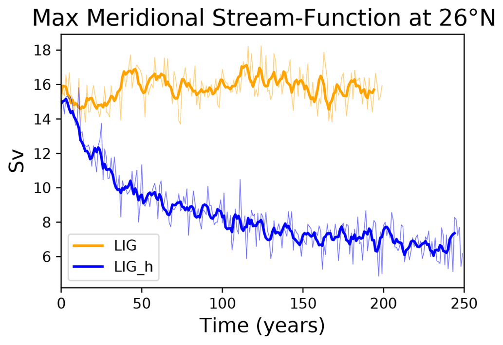
Figure 1 Maximum meridional streamfunction at 26^∘ N for LIG (orange) and LIG_hosing (blue). Thin lines are annual means, thick lines are 11-year running means.

The freshwater forcing has a large impact on the temperature structure of the upper ocean. The North Atlantic top ocean layer (top 200 m) cools down by $\sim -\mathrm{0.8}$ ^∘C within the first 50–80 years and remains approximately constant (Fig. 2a) thereafter. However, as the ocean below 200 m warms, the overall temperature of the top ∼1 km of the ocean remains approximately unchanged with a small net warming of ∼0.1 ^∘C by the end of the 250 years of LIG_hosing simulation (Fig. 2c).

This pattern of cooling and warming in the Northern Hemisphere (NH) ocean surface and subsurface layers, respectively, is consistent with the combined effects of the freshening of the North Atlantic Ocean and the slowdown of the meridional overturning circulation (Fig. 1). As the AMOC weakens, less heat is transported northward. This causes a surface cooling of the Northern Hemisphere (see Fig. S1 in the Supplement, see also Sect. 3.3 for a detailed discussion on the ocean heat transport). At the same time, the enhanced freshwater flux in the North Atlantic is responsible for a freshening of the ocean surface layers (Figs. S10 and S11) that disrupts deep convection and substantially thins the mixed layer in the region (Fig. S8). In the absence of any vertical mixing, the colder fresher surface waters do not mix with the warmer subsurface waters and the ocean underneath is warmer in the hosing experiment compared to the LIG (Fig. S1); this also contributes to a further cooling of the ocean surface in the LIG_hosing simulation.

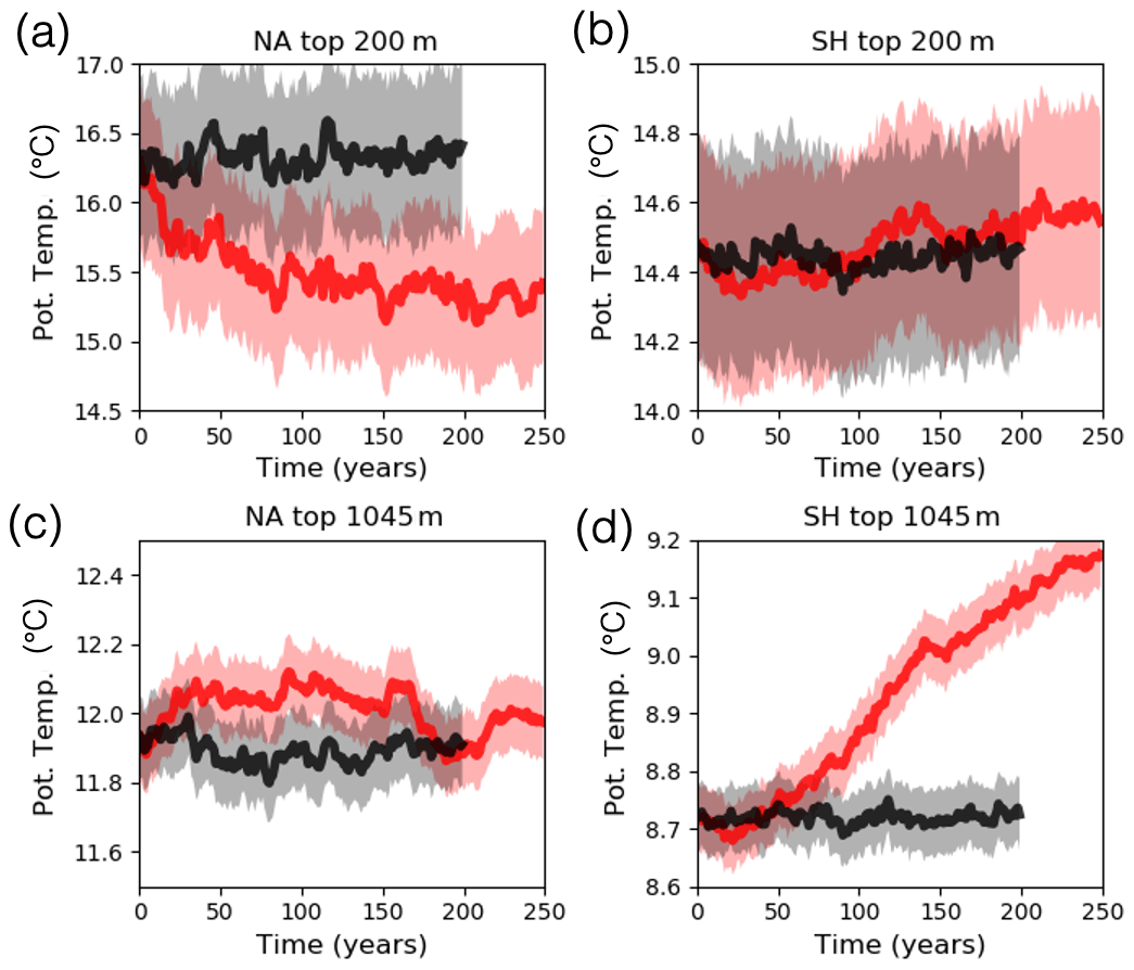
Figure 2 North Atlantic (NA) and Southern Hemisphere (SH) depth-averaged means of seawater potential temperature for LIG_hosing (red) and LIG (black). (a, b) Averages over the top 200 m of the water column, (c, d) averages over the top 1045 m of the water column. Thick lines are annual means, shaded areas represent the standard deviation.

In the Southern Hemisphere (SH), whilst the top 200 m of the ocean warms by $\sim +\mathrm{0.15}$ ^∘C (Fig. 2b), the top 1 km of the ocean warms by $\sim +\mathrm{0.5}$ ^∘C (Fig. 2d) after 250 years. This is due to the weakened global meridional overturning circulation. We estimate a warming trend of ∼0.2 ^∘C per 100 years in the upper 1 km of the ocean (Fig. 3a). The warming trend is present at the end of 250 years, implying that the system is still far from a new equilibrium. The SH warming is most intense at low latitudes and near the Equator (Fig. 3b). At high southern latitudes, cold ocean surface LIG_hosing–LIG anomalies occur at the edge of the Antarctic sea ice edge. We explore this behaviour in Sect. 3.3.2.

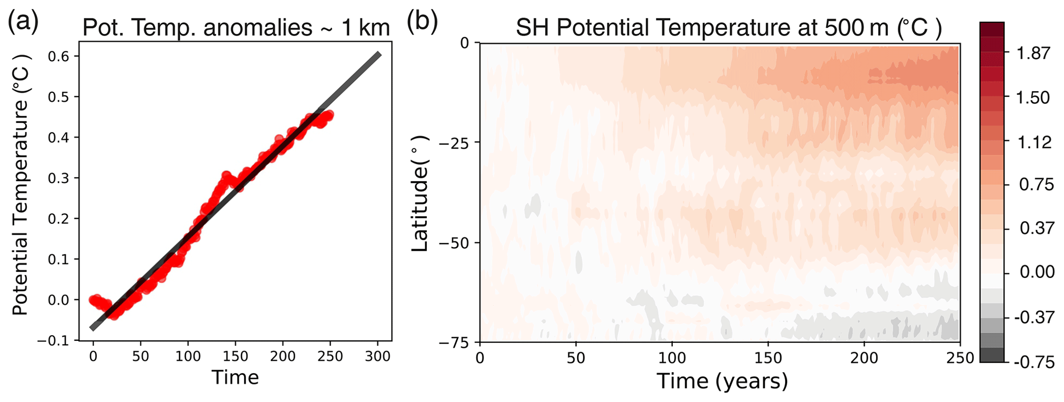
Figure 3 Southern Hemisphere seawater potential temperature anomalies: (a) depth-averaged LIG_hosing–LIG anomalies over the top 1045 m of the water column and linear fit, (b) Hovmöller diagram of LIG_hosing–LIG anomalies at 500 m depth.

3.2 Atmospheric changes

The large-scale atmospheric circulation is related to the horizontal temperature gradient by the thermal wind relation. Changes in the meridional temperature gradient at the surface can influence the wind field above by modulating the strength of the vertical wind shear (i.e. the rate at which the wind changes with height) and the latitudinal position of the wind maximum (i.e. the jet stream location).

In the Northern Hemisphere, ocean surface cooling increases the pole-to-Equator temperature difference and therefore the strength of the meridional temperature gradient compared to the LIG (Figs. 4a and 5a). The largest differences are found in the 40–55^∘ N region. At 50^∘ N, the temperature gradient is $\sim -\mathrm{0.4}$ ^∘C per 100 km for LIG_hosing – this is double the LIG $\sim -\mathrm{0.2}$ ^∘ per 100 km gradient (Fig. 5a). During the first 10 years of hosing simulation, surface air temperature (SAT) anomalies are weakly negative at mid-latitudes and high northern latitudes and close to zero near the Equator (dark blue curve in Fig. 6b). Over time, as negative SAT anomalies build up in the Northern Hemisphere, the jet stream progressively increases its strength (curve colours transition from blues to reds in Fig. 6a and b). The upper-level climatological zonal wind anomalies are ∼2 m s⁻¹ stronger in LIG_hosing than in LIG. Because the wind shear associated with the mid-latitude jet stream extends to the surface (Fig. 6c), the stronger LIG_hosing near-surface winds are a consequence of the jet intensification above (Figs. 4b and 5b).

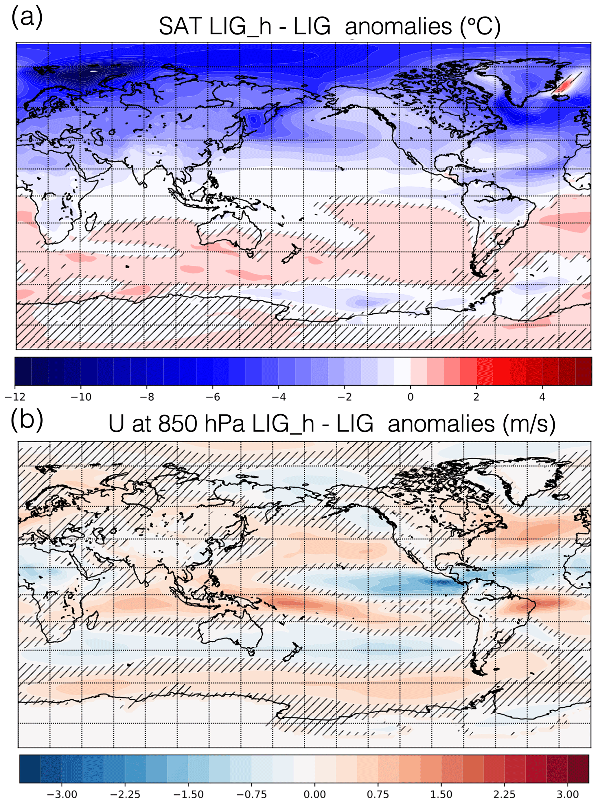
Figure 4 LIG_hosing–LIG surface air temperature (SAT) anomalies (a) and zonal mean U at 850 hPa anomalies (b). Non-hatched areas correspond to statistically significant differences (at 95 % confidence).

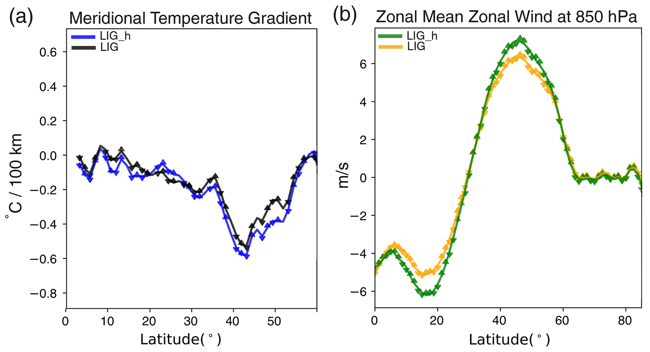
Figure 5 Mean surface air temperature (SAT) meridional temperature gradient for LIG_hosing (blue) and LIG (black) (a) as well as zonal mean zonal wind U at 850 hPa for LIG_hosing (green) and LIG (orange) (b) for the North Atlantic (80–10^∘ W) region. Solid lines are annual means, arrows are the standard error of the mean.

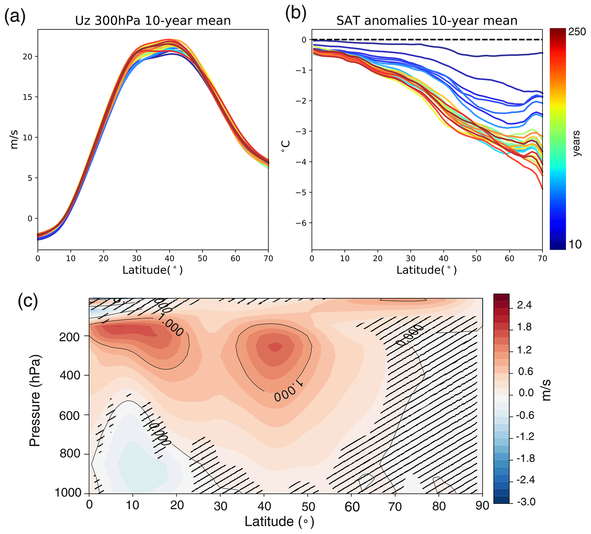
Figure 6 Each line in panel (a) corresponds to a 10-year mean of the zonal mean zonal wind U at 300 hPa for the LIG_hosing run. Similarly, in panel (b), each line represents a 10-year mean of LIG_hosing–LIG surface air temperature (SAT) anomalies. Panel (c) shows the long-term mean of zonal mean zonal wind LIG_hosing–LIG anomalies. Non-hatched areas correspond to statistically significant differences (at 95 % confidence).

The strength, shape, and location of the jet stream are highly variable on a year-to-year basis. This is due to factors such as season differences, rates of tropical heating and high-latitude cooling, and stratospheric conditions. The flow regime can be a single or double jet regime depending on whether the subtropical and mid-latitude jets are joined together or whether they are distinguishable as separate entities (Lee and Kim, 2003; Son and Lee, 2005; Lachmy and Harnik, 2014). These variations, over all timescales, mean the climatological jet maximum is spread out approximately across 20^∘ of latitude (Fig. 6a and c).

Finally, note that although we have only shown annual means here, a similar behaviour for the jet stream, the near-surface winds, and the meridional temperature gradient was observed in the seasonal means. According to the jet stream dynamics and the fact that the pole-to-Equator temperature difference is always stronger in winter and weaker in summer, the largest LIG_hosing–LIG anomalies occur during the winter and spring seasons (see Figs. S2–S5).

In the Southern Hemisphere, whilst the surface warming is weak (Figs. 4a and 7b), zonal wind anomalies are nevertheless significant (Fig. 7a and c). Zonal wind anomalies reach values of $\sim -\mathrm{2}$ to 3 m s⁻¹ at low latitudes to mid-latitudes – in the 30–40^∘ S region. At higher southern latitudes, values of $\sim +\mathrm{1}$ m s⁻¹ occur.

Figure 7 As in Fig. 6 but for the Southern Hemisphere.

While the surface warming observed in the Southern Hemisphere subtropics has the potential to generate negative wind anomalies at mid-latitudes via a mechanism similar to the one discussed above for the Northern Hemisphere, i.e. by decreasing the meridional temperature gradient between tropics and subtropics and thus weakening the subtropical jet (Brayshaw et al., 2008; Yang et al., 2020), the positive surface temperature anomalies in Fig. 7b are too small to explain these simulated wind changes. We require an additional mechanism in our simulation that explains the weakened subtropical jet.

Several studies have investigated latitudinal shifts of the Intertropical Convergence Zone (ITCZ) following a cooling at high latitudes of the Southern and Northern Hemisphere (Kang et al., 2008; Donohoe et al., 2013; Lee et al., 2011; Ceppi et al., 2013). These have established the cause–effect relationships between temperature changes, ITCZ displacement, and Hadley cell strength. Changes in the inter-hemispheric meridional temperature (and pressure) gradient cause the ITCZ to shift towards the warmer hemisphere; in the colder hemisphere, the Hadley cell strengthens because of the enhanced cross-equatorial transport of momentum, and in the warmer hemisphere the other Hadley cell weakens. Here, we assess the ITCZ mean meridional position by looking at LIG_hosing–LIG precipitation anomalies (Fig. 8). In the LIG_hosing simulation, the ITCZ moves southward as the Northern Hemisphere cools. The long-term mean anomalies are $\sim \pm$2 mm d⁻¹ in both hemispheres (Fig. 8b). The southward shift of the ITCZ disrupts the SH subtropical jet, which is weaker in the hosing simulation compared to the LIG (Fig. 7c).

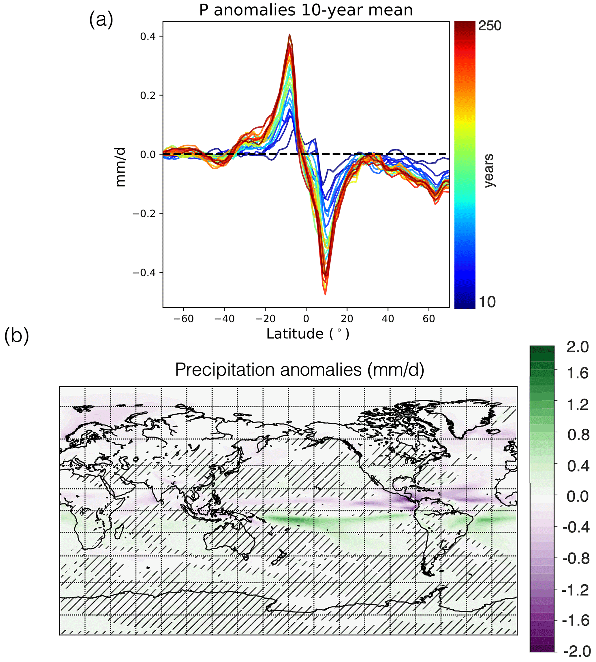
Figure 8 Each line in panel (a) corresponds to a 10-year mean of LIG_hosing–LIG precipitation (P) anomalies. In panel (b), the long-term mean of P anomalies is shown. Non-hatched areas correspond to statistically significant differences (at 95 % confidence).

Because of the weak subtropical jet, baroclinic eddy growth is strong at mid-latitudes, and this drives a strong polar (eddy-driven) jet (Lee and Kim, 2003). The system moves towards a split jet regime: the HadGEM3 polar and subtropical jets are distinguishable as two separate peaks in the zonal mean zonal wind (Fig. 7a and c), with the polar (subtropical) jet stronger (weaker) in LIG_hosing than in LIG. This strengthening of the LIG_hosing simulation polar jet has consequences for the high-latitude surface circulation and also has impacts on Antarctic sea ice.

3.3 Coupled system responses

In the previous sections, we focused our analysis on the direct impacts of the freshwater surface forcing on the ocean and the atmosphere. Because they originate from a perturbation applied as a boundary condition between the ocean and the atmosphere (i.e. the applied meltwater), the changes discussed so far can be simulated by stand-alone oceanic or atmospheric simulations. In this section, we look at how the atmosphere and ocean systems interact with each other to give rise to additional modifications of the climate system that can only be assessed in a coupled model simulation framework.

3.3.1 Heat transport changes

In the LIG_hosing simulation, the total advective heat transport decreases everywhere in the Atlantic basin (Fig. 9b). The major drop ($\sim -\mathrm{0.25}$ PW) occurs during the first 50 years of simulation (Figs. 9c and S6a). The temporal evolution of the Atlantic advective heat transport resembles the AMOC trend (Fig. 1), with values reaching a plateau (∼0.4 PW, or −33 % change) near year 150 of simulation. In the Northern Hemisphere, the largest decrease is $\sim -\mathrm{0.4}$ PW at about 10^∘ N (Fig. 9b). In the Southern Hemisphere, the difference in Atlantic advective heat transport between the LIG_hosing and LIG simulations is about −0.25 PW between the Equator and 35^∘ S (at the end of the Atlantic). This means that some combination of the Indian, Pacific, and Southern oceans is taking up an additional 0.25 PW of ocean heat transport in the LIG_hosing simulation that was being lost in the North Atlantic in the LIG simulation. This explains the LIG_hosing warming at the surface (Fig. 4a) and at 500 m depth (Fig. 3b) at those latitudes, since extra heat is being stored by the ocean.

Figure 9 Total advective (a–c), overturning (d–f), and gyre (g–i) northward heat transport for the global basin (a, d, g), the whole Atlantic basin (b, e, h), and the North Atlantic basin only (c, f, i) for the LIG_hosing and LIG simulations. Panels (a), (b), (d), (e), (g), and (h) show zonal means computed over the long-term means. Panels (c), (f), and (i) show area-weighted annual time series.

The overturning heat transport component (Fig. 9e and f), which is largely density-driven, is the major contributor to the overall decrease in Atlantic advective heat transport (also referred to here as total northward heat transport). This component is directly linked to the strength of the meridional overturning circulation, and its decrease is uniform across all latitudes. On the other hand, the wind-driven gyre heat transport component exhibits a far less uniform trend (Fig. 9h and i).

Northern Hemisphere westerly winds are about 20 % stronger in the LIG_hosing simulation. The maximum positive zonal wind anomaly is centred in the 40–50^∘ N latitude band (Fig. 5b), consistent with the jet stream intensification (Fig. 6c). This is roughly where the boundary between the subpolar and subtropical gyres is located (Fig. 10). The barotropic streamfunction weakens in the subpolar gyre for the LIG_hosing simulation because the enhanced westerlies act to decelerate the counterclockwise rotation (barosf negative) of the gyre. At the same time, the subtropical gyre intensifies as the stronger westerly winds favour the clockwise (barosf positive) rotation of the gyre in that region. Because of the location of the maximum wind anomaly between 40–50^∘ N, the stronger westerlies impact the subpolar gyre more greatly than the subtropical gyre in terms of gyre shape. The southern branch of the subtropical gyre is also affected by wind changes. The barotropic streamfunction for the LIG_hosing subtropical gyre strengthens in the 20–30^∘ N region (particularly in the western quadrant) because of the modest acceleration in the easterly trade winds (Fig. 5b). The net result is an overall weakening of the subpolar gyre and an intensification of the subtropical gyre in the LIG_hosing simulation compared to the LIG. This results in a decrease in heat transport due to the gyre circulation of $\sim -\mathrm{0.2}$ PW at high northern latitudes between 50–60^∘ N but an increase of $\sim +\mathrm{0.1}$ to 0.2 PW over mid-latitudes in the 20–50^∘ N region (Fig. 9h).

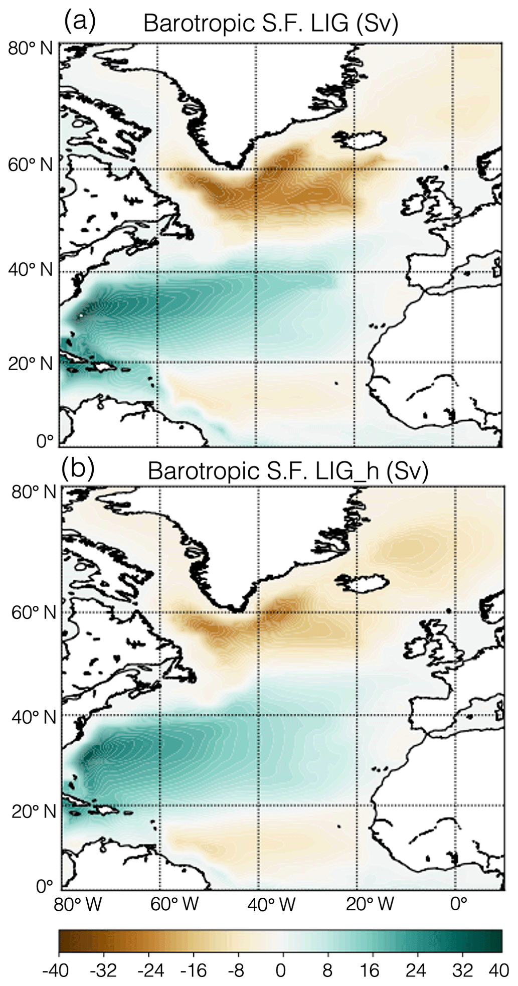
Figure 10 The annual mean barotropic streamfunction in the North Atlantic for the LIG (a) and the LIG_hosing (b) simulations.

The weakening and strengthening of the subpolar and subtropical gyres approximately balance in terms of total gyre heat transport: the total northward transport of heat due to the gyre circulation in the North Atlantic (with contributions from both gyres) is nearly unchanged by the meltwater forcing (Fig. 9i). However, the implications of a different regional distribution of ocean heat are of significance. If the response of the coupled system, i.e. changes in the gyre heat component, were not simulated, a larger reduction in total advective heat transport would occur at mid-latitudes. Furthermore, the decrease in total advective heat transport at high northern latitudes (Fig. 9b), north of 50^∘ N, would be non-existent. This is because the overturning heat transport term is zero above 50^∘ N (Fig. 9e); i.e. the decrease comes from the weakening of the subpolar gyre (Fig. 9h). The weakened subpolar gyre thus contributes to the large ocean surface cooling of the North Atlantic (Fig. 4a). This process is not usually taken into consideration when models are used to explain the cooling of the Northern Hemisphere during hosing experiments simulating Heinrich events.

We conclude this section by highlighting that changes in the Atlantic basin heat transport terms discussed above dominate the signal also in the global ocean heat transport terms (Fig. 9a, d and g). The opposite response of the subtropical and subpolar gyres is still present when the global gyre heat transport term is computed. As for the overturning component, this is still mainly responsible for the decrease in global heat transport, but south of 10^∘ N heat gain in the Pacific (Fig. S12) reduces LIG and LIG_hosing differences in the overturning and advective global heat transport terms. South of ∼55^∘ S there is no difference in the global advective heat transport for the two runs. This indicates that in our 250-year-long simulation, the freshwater forcing results in heat accumulation in the Southern Ocean between the Equator and ∼55^∘ S, but no heat is transported (and no heat accumulates) southwards of 55^∘ S (see also Sect. 4).

3.3.2 Southern Hemisphere sea ice changes

The net effect of a weakened Southern Hemisphere subtropical jet (caused by the southward shift of the ITCZ) is to intensify the Southern Hemisphere polar jet and the surface winds (Fig. 11a and b), which results in a more positive Southern Annular Mode (SAM) (Fig. 11c). Winds are stronger in the LIG_hosing simulation than in the LIG, with wind anomalies at 850 hPa up to +1 m s⁻¹ (Fig. 11b). The time progression of the wind intensification shown in Fig. 11a and b is in agreement with the temporal evolution of the ITCZ shift discussed in Sect. 3.2 and shown in Fig. 8. As the belt of westerly winds becomes stronger, the SAM becomes more positive. The mean value for the SAM index (non-standardized) is −0.05 hPa for the first 150 years of simulation (Fig. 11a) and 0.4 hPa for the last 100 years of simulation (Fig.  11b), resulting in a positive trend for the annual SAM index (Fig. 11c).

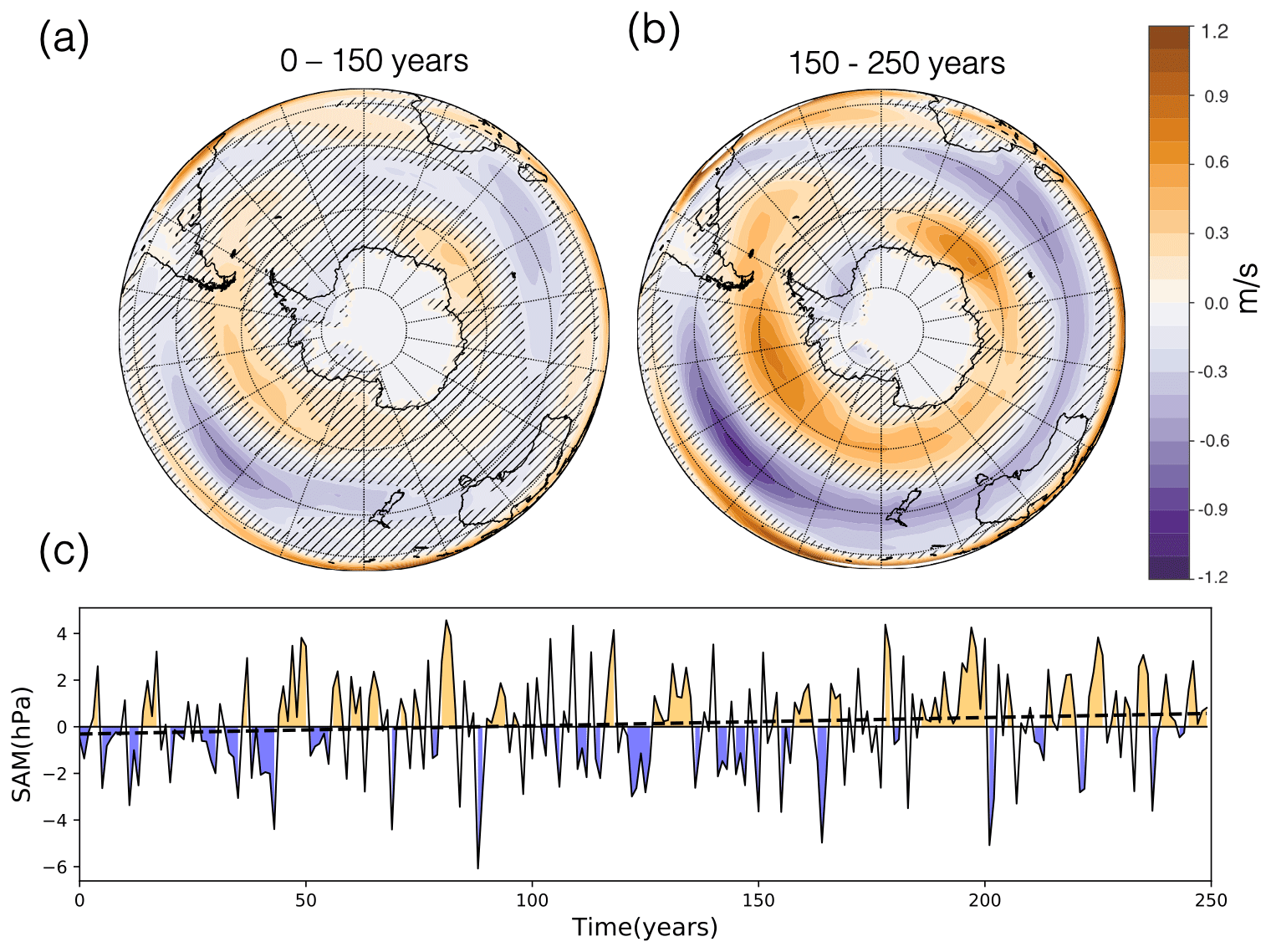
Figure 11 LIG_hosing–LIG anomalies for U at 850 hPa computed over the first 150 years (a) and the last 100 years (b) of simulation. Non-hatched areas correspond to statistically significant differences (at 95 % confidence). The annual SAM index for the LIG_hosing simulation is shown in (c). The linear regression line (dashed) represents a statistically significant positive trend with a p value < 0.05.

Here, we find that in response to an increasingly positive SAM, in our LIG_hosing simulation, the Southern Hemisphere sea ice expands with maximum LIG_hosing–LIG winter sea ice concentration (SIC) anomalies of $\sim +\mathrm{30}$ % (Fig. 12c). Positive anomalies are in fact present all year round, but are weaker in summer (Fig. 12a) and the annual mean SIC anomalies are $\sim +\mathrm{20}$ % at most (Fig. 12e).

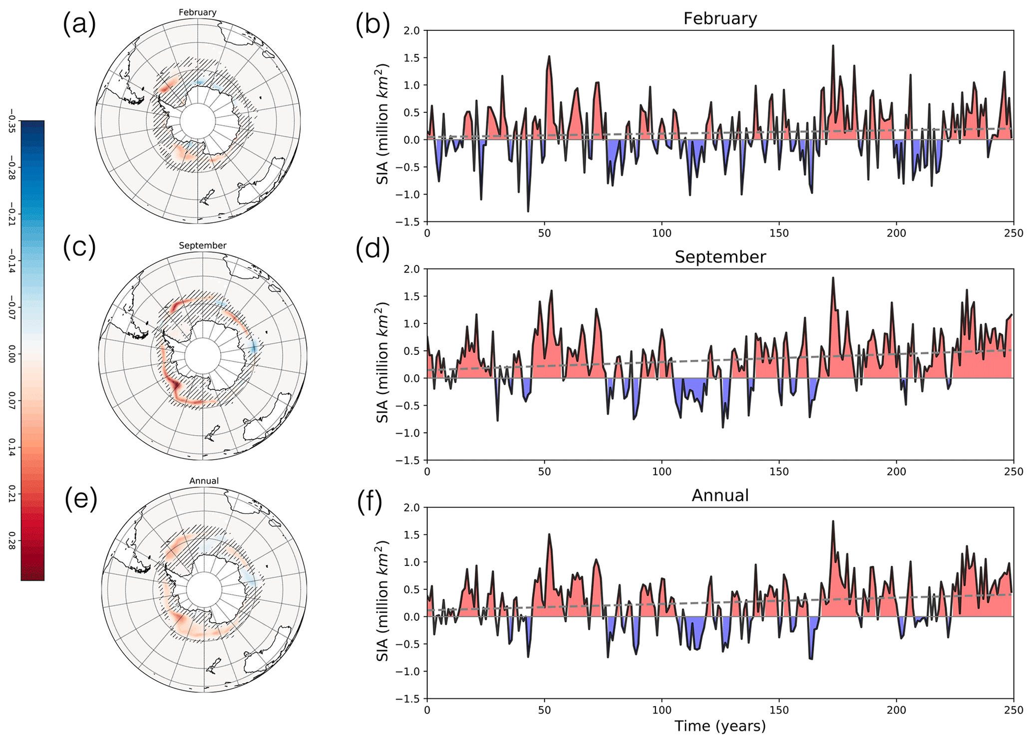
Figure 12 February (a), September (c), and annual (e) LIG_hosing–LIG sea ice concentration (SIC) anomalies for the last 100 years of the LIG_hosing simulation. Non-hatched areas correspond to statistically significant differences (at 95 % confidence). Panels (b), (d), and (f) are time series of February (b), September (d), and annual (f) LIG_hosing–LIG sea ice area (SIA) anomalies computed against the LIG climatological mean from year 0 to 250 of simulation. Dashed grey lines represent best fit for data. The trend is positive and statistically significant (p value < 0.05) for September (d) and annual (f) time series and still positive but not significant (p value > 0.05) for the February (b) time series.

The connection between a positive SAM and an increase in Antarctic sea ice is widely reported in the literature (e.g. Hall and Visbeck, 2002; Lefebvre et al., 2004; Ferreira et al., 2015; Turner et al., 2015; Holland et al., 2017). Known mechanisms by which a positive SAM can influence sea ice formation and growth are as follows: the stronger westerly winds advect sea ice away from the coastlines more efficiently and thus increase the ice concentration along the ice edge (Fig. 12) (Hall and Visbeck, 2002; Lefebvre et al., 2004); the enhanced westerlies can cause an anomalous equatorward Ekman flow that, advecting colder water from the south, decreases the sea surface temperature (SST) and promotes sea ice formation (Ferreira et al., 2015; Holland et al., 2017).

The temporal evolution of the SAM index (Fig. 11) and the sea ice area (SIA) anomalies (Fig. 12b, d and f) corroborates that sea ice changes in our LIG_hosing simulation are SAM-driven: in the last ∼100 years of simulation, as 850 hPa winds intensify and the SAM is more frequently positive (Fig. 11), SIA anomalies are mostly positive and their magnitude is slowly increasing too (although not in summer, see below). This is confirmed by the overall positive trend of the time series (dashed lines in Fig. 12). The LIG_hosing sea ice area increases more substantially in the second half of the simulation, under a prevalently positive SAM regime. The overall trend for winter (Fig. 12d) and annual (Fig. 12f) SIA anomalies time series is positive and statistically significant (p value < 0.05). In summer (Fig. 12b), however, the trend is still (weakly) positive but not statistically significant (p value > 0.05). This reveals that sea ice changes are driven by winter changes; i.e. the positive trend is visible in the September time series but not in February, agreeing with what we know about the seasonality of SAM–sea ice interactions. Studies have shown that the link between SIC anomalies and SAM is strongest during the winter months, particularly in the Pacific sector where sea ice variability is strongly linked to the large-scale atmospheric circulation (see e.g. Simpkins et al., 2012).

Often in the literature a positive SAM index is associated with a dipole pattern of SIC anomalies, for which sea ice decreases in the Weddell Sea sector and increases in the Amundsen and Ross Sea sectors (Lefebvre et al., 2004; Simpkins et al., 2012). This pattern is not clearly distinguishable in our results, where sea ice rather increases along the ice edge in both the Weddell and the Amundsen and Ross Sea sectors. In the central Weddell Sea, the increase is accompanied by some zero or mildly positive or negative anomalies off the peninsula. While it is not clear why a strong dipole pattern of anomalies is not present in our simulation, other processes might affect sea ice concentration in the Weddell Sea sector for our LIG_hosing run: upwelling of cold waters in the Southern Ocean between 40 and 70^∘ S has been postulated as an explanation for the increase of sea ice in the Weddell Sea sector in response to a North Atlantic cooling (Crowley and Parkinson, 1988). This mechanism was invoked by Renssen et al. (2010) to explain positive SH sea ice anomalies during the early Holocene deglaciation (∼9000 years ago). In our simulation, the ocean zonal mean temperature anomalies are different from Renssen et al. (2010): at depth, the Southern Ocean warms near 40^∘ S (Figs. 3 and S1). We also found either zero or very small negative temperature anomalies between 50–70^∘ S at the surface (Fig. S1). This implies that some very weak upwelling of cold waters might be happening in the HadGEM3 model and could contribute to the sea ice increase in the Weddell Sea sector. The very weak upwelling of cold waters in the Southern Ocean in our simulation is supported by the fact that the expected lag between North Atlantic cooling and SH cold waters upwelling is 100–200 years (Goosse et al., 2004; Renssen et al., 2010), but HadGEM3 was run here for 250 years.

4 Discussion

The observational record from the LIG suggests that by around 128 ka, after a 4000–5000-year Heinrich 11 event, there should be 2–3 ^∘C ocean warming at high southern latitudes (Capron et al., 2014, 2017; Hoffman et al., 2017). The positive warming trend of ∼0.2 ^∘C per 100 years of Fig. 3 implies that, after 250 years of meltwater forcing, the Southern Hemisphere is still warming in our LIG_hosing simulation (see also Sect. 3.1). If one extrapolates, using a linear fit to Fig. 3, after ∼1500 years, the model may simulate a 2–3 ^∘C warming. In this regard, our results are somewhat similar to previous studies like Holloway et al. (2018), who ran a 1600-year-long simulation with the older HadCM3 model and obtained a $\sim +\mathrm{1.5}$ ^∘C warming. However, we must be cautious about extrapolating thousands of years from a 250-year simulation: this linear trend may not be sustained in the long term towards equilibrium.

In our LIG_hosing simulation, the warming of the Southern Ocean is driven by a redistribution of ocean heat. After 150 years of simulation, the AMOC is reduced by around 60 %; therefore considerably less heat is being lost in the NH each year, which leads to a continual gradual build of heat elsewhere in the ocean.

The changes in the North Atlantic heat transport terms (gyre and overturning components) discussed in Sect. 3.3.1 are responsible for the NH cooling and SH warming, and they also dominate the signal in the global ocean heat transport terms (Fig. 9). Regarding gyre changes, it is worth pointing out that previous studies have associated the asymmetry between the subpolar and the subtropical gyre, similar to the asymmetry observed here, to a leakage of freshwater from subpolar latitudes into subtropical waters (Swingedouw et al., 2013). While a leakage of freshwater signal cannot be ruled out for the HadGEM3 model (Menary et al., 2018), in previous hosing experiments showing leakage the intensity of both the subpolar and subtropical gyres decreased over time (with the subtropical gyre only marginally affected). Furthermore, in these experiments, the freshwater forcing was exclusively applied along the Greenland coastline (Swingedouw et al., 2013). Our uniform release of freshwater in the 50–70^∘ N latitudinal band should not encourage freshwater leakage through the oceanic pathways described by Swingedouw et al. (2013), and, most importantly, the strengthening of the subtropical gyre in our LIG_hosing simulation is a major difference from Swingedouw et al. (2013), corroborating that alterations to the gyre circulation in the LIG_hosing run are driven by wind changes.

Regarding sea ice changes, the positive SAM and the larger sea ice concentration found in our LIG_hosing simulation are findings consistent with each other and are in agreement with the literature on the subject. However, positive SIC anomalies for the LIG_hosing simulation put our findings in contrast with the hypothesis that, during the Last Interglacial, the SH sea ice began to decline following the Heinrich 11 event (Holloway et al., 2018). This hypothesis is based on the assumption that ocean heat would build up in the Southern Ocean in response to the weakened overturning meridional circulation.

Over the first 250 years of their water-hosing simulation, Holloway et al. (2018) show that in HadCM3 (older UK model), SH winter sea ice goes into immediate decline, and after 200 model years, the sea ice area anomaly is $\sim -\mathrm{10}$ % (see their Fig. 1). This older HadCM3 model has a rather simplified representation of the atmosphere and the ocean compared to HadGEM3 (HadCM3 is the predecessor of HadGEM3 with about 20 years of model development between them).

In our 250-year-long simulation, while freshwater forcing has an immediate major impact on the (North and South) Atlantic basin (Fig. 9b), the global heat transport south of 55^∘ S remains unaffected (Fig. 9a). Thus, in our simulation, sea ice does not respond to changes in ocean heat transport (yet) but rather to shorter timescale forcing such as the SAM. This is in agreement with previous studies showing the existence of an approximately 200-year lag between changes in freshwater forcing from Greenland and the onset of warming in Antarctica since the warming signal takes time to cross the Antarctic Circumpolar Current (at about 50–60^∘ S) (Buizert et al., 2015; Pedro et al., 2018; Svensson et al., 2020).

As described in Sect. 3.3.2, a more positive SAM in the LIG_hosing run causes an increase in SH sea ice in HadGEM3. However, on longer timescales it is possible, and perhaps likely, that sea ice might start responding to a more pronounced warming of the Southern Ocean (according to trend of Fig. 3) and that could eventually start declining: a much warmer Southern Ocean will inhibit sea ice formation and will contribute to faster sea ice melt. Additionally, the SAM may transition into a different state. For example, the weak subtropical warming observed at the ocean surface in our LIG_hosing simulation has the potential (if enhanced) to further weaken the subtropical jet (see Sect. 3.2) and move the system into a proper split jet regime in which the subtropical jet and the polar jet are distinguishable. This would result in an even stronger polar jet and thus a more positive SAM, which might reinforce the role of the SAM in promoting sea ice increase. A longer simulation would allow a proper investigation of such mechanisms.

Similarly to the above, a longer simulation with a more pronounced ocean warming would allow investigating other noteworthy aspects, which include the following.

• If the Southern Ocean continues to warm towards +3 ^∘C warming, the pattern of warming will be of importance (Brayshaw et al., 2008). A homogeneous warming that extends to the higher latitudes might disrupt and weaken the polar jet (by decreasing the polar to mid-latitude meridional temperature gradient). Under this scenario, the SAM will polarize towards its negative phase and sea ice could decrease.

• Even with a SAM persistently positive, a two-timescale evolution of sea ice is possible. First proposed by Ferreira et al. (2015), following an initial sea ice increase (according to the mechanisms discussed here), on longer timescales, sea ice is expected to decrease when the SAM is positive. This is because, on long timescales, the deeper ocean circulation is also affected by the changes in the wind forcing. In particular, the upwelling of deeper and warmer ocean waters will eventually increase the SST and melt the sea ice.

To conclude, we hypothesize that the positive SIC anomalies in Fig. 12 are partially due to the limited length of our simulation (250 years). It is well known that the ocean system responds to forcing on timescales that can be longer than 1000 years. We speculate that, for a longer LIG_hosing simulation, the weak warming signal currently observed in the Southern Hemisphere might become larger and a more significant warming of the Southern Ocean might be simulated (according to Fig. 3).

In this perspective, the positive trend in the SAM and the slowdown of the AMOC might be thought of as two competitive mechanisms that cause sea ice to increase or decrease depending on the process that is dominating the sea ice response. Our findings thus suggest that there might be a transient system response for which sea ice actually increased its extent during the LIG for a few hundred years (or more).

However, without prolonging our simulation, it is not possible to investigate how these two mechanisms might interact with each other. Thus, whilst a longer LIG_hosing simulation using our model is difficult due to the prohibitively high computational cost, supercomputing advances are needed to enable a more in-depth investigation of some of the mechanisms described here for Southern Ocean warming and Antarctic sea ice increase. Until this is possible, longer-term hemispheric teleconnections, Southern Ocean warming, and when and how Antarctic sea ice disappeared during the Last Interglacial may remain somewhat elusive.

5 Conclusions

In this study, we have analysed the response of the ocean and the atmosphere to an enhanced release of glacial meltwaters within the North Atlantic basin during the Last Interglacial (LIG) period. We found two noteworthy aspects of how the applied freshwater forcing alters the atmosphere–ocean coupling; these are changes in the Northern Hemisphere gyre heat transport and an increase in Antarctic sea ice.

We used the UK CMIP6 model (HadGEM3) to simulate a time slice of the Last Interglacial climate at 127 000 years ago (LIG simulation) (Guarino et al., 2020a). A constant flux of freshwater equal to 0.2 Sv was added to the North Atlantic between 50–70^∘ N to study the sensitivity of the LIG climate to the glacial meltwater release (LIG_hosing simulation). This simulation was carried out by adhering to the international protocol for the PMIP4-LIG Tier 2 simulations (Otto-Bliesner et al., 2017).

After 150 years of freshwater forcing, the Atlantic Meridional Overturning Circulation (AMOC) is reduced by about 60 %. After a steady decline, and for the last 100 years of simulation, the AMOC remains approximately constant at around 9 Sv.

The combined action of a fresher North Atlantic Ocean and a weaker meridional overturning circulation leads to a pattern of cooling and warming in the Northern Hemisphere ocean surface and subsurface, respectively, that is in agreement with previous studies (Stocker et al., 1992; Clark et al., 1999; Knutti et al., 2004; He et al., 2020). In the Southern Hemisphere, both the ocean surface and subsurface warm, with an estimated trend of ∼0.2 ^∘C per 100 years in the upper 1 km of the ocean. This trend remains approximately linear and constant for 250 years. After 250 years (length of simulation), the warming trend is continuing and the system has not reached a new equilibrium.

The pole-to-Equator temperature difference increases in the LIG_hosing simulation compared to the LIG simulation in the Northern Hemisphere due to polar cooling. The largest increase in the meridional surface temperature gradient between LIG and LIG_hosing occurs between 40–50^∘ N. These changes in the meridional temperature gradient at the surface influence the wind field. In the LIG_hosing simulation, 850 hPa winds are found to be ∼20 % stronger with a maximum positive anomaly centred at 45^∘ N. This is a direct consequence of the intensification of the jet stream above that is ∼2 m s⁻¹ stronger in the LIG_hosing simulation than in the LIG simulation.

The jet intensification in the Northern Hemisphere alters the total northward ocean heat transport (i.e. the advective heat transport) by increasing and decreasing the gyre circulation at mid-latitudes and high latitudes, respectively. At mid-latitudes, increased subtropical gyre circulation means that this part of the ocean circulation transports more heat northward. At the same time, the weakening of the overturning circulation in the same region reduces northward overturning heat transport. Whilst these two elements act in opposite direction, the overturning component effect dominates so that the total advective heat transport decreases in the hosing experiment compared to the reference LIG climate. At higher latitudes in the Northern Hemisphere, the contribution to the total advective heat transport from the overturning circulation is zero, and in this case, it is the weakening of the subpolar gyre that makes the total advective heat transport decrease in this region for the LIG_hosing simulation. The weakened subpolar gyre is thus, in our LIG_hosing simulation, an additional contributor to the cooling of the ocean surface in the North Atlantic. This process should be taken into account when studying the cooling of the Northern Hemisphere in water-hosing simulations representing Heinrich events.

As the Northern Hemisphere cools down, the changes in meridional temperature and pressure gradients cause the Intertropical Convergence Zone (ITCZ) to move southward with precipitation anomalies equal to $\sim \pm \mathrm{2}$ mm d⁻¹ in the Southern and Northern Hemisphere. In the Southern Hemisphere, the shift of the ITCZ disrupts the SH subtropical jet, which weakens. A weakening of the subtropical jet ($\sim -\mathrm{2}$ to 3 m s⁻¹) corresponds to a strengthening of the polar jet ($\sim +\mathrm{1}$ m s⁻¹), and the system moves towards a split jet regime.

The SH polar jet intensification leads to stronger westerlies and to Southern Annual Mode (SAM) changes. The SAM exhibits a positive trend and becomes more positive overall during the last 100 years of LIG_hosing simulation. A positive SAM influences sea ice formation through dynamical feedbacks and acts to increase Antarctic sea ice in the LIG_hosing simulation. We speculate that the SH sea ice increase that our model captures may be part of a two-stage Antarctic sea ice response to the meltwater release (see Sect. 4). Highly resolved records of Last Interglacial changes from the Southern Ocean could be examined for evidence of this occurrence. This knowledge should also be of value to the paleoclimate proxy community in interpreting current contrasting sea ice observations (e.g. Chadwick et al., 2020).

As discussed above, 250 years are not enough for all the possible climate processes governing the LIG climate to manifest. Since the present article was first written, the HadGEM3 LIG_hosing simulation presented here has been extended by a further ∼100 years. By analysing these additional model years, we found no differences in terms of model behaviour and climate system response to the applied freshwater forcing. This is not surprising, since the different climate responses discussed above are likely to fully manifest on much longer timescales (than a few hundred years) because of their dependency on the ocean response (as detailed in the Discussion section). The HadGEM3 LIG_hosing simulation is currently being extended even further, and results from the extended run will be the subject of further studies.

Finally, we note that gyre changes and SH sea ice increase significantly shape and influence the LIG climate in our hosing simulation, and, as shown here, they can only be assessed in a coupled model simulation framework.