the Creative Commons Attribution 4.0 License.
the Creative Commons Attribution 4.0 License.
 | 29 Mar 2023
A 258-year-long data set of temperature and precipitation fields for Switzerland since 1763
Noemi Imfeld
Lucas Pfister
Yuri Brugnara
Stefan Brönnimann
Climate reconstructions give insights in monthly and seasonal climate variability in the past few hundred years. However, for understanding past extreme weather events and for relating them to impacts, for example through crop yield simulations or hydrological modelling, reconstructions on a weather timescale are needed. Here, we present a data set of 258 years of daily temperature and precipitation fields for Switzerland from 1763 to 2020. The data set was reconstructed with the analogue resampling method, which resamples meteorological fields for a historical period based on the most similar day in a reference period. These fields are subsequently improved with data assimilation for temperature and bias correction for precipitation. Even for an early period prior to 1800 with scarce data availability, we found good validation results for the temperature reconstruction especially in the Swiss Plateau. For the precipitation reconstruction, skills are considerably lower, which can be related to the few precipitation measurements available and the heterogeneous nature of precipitation. By means of a case study of the wet and cold years from 1769 to 1772, which triggered widespread famine across Europe, we show that this data set allows more detailed analyses than hitherto possible.
- Article
(9783 KB) - Full-text XML
-
Supplement
(381 KB) - BibTeX
- EndNote


Reconstructions of atmospheric variables on monthly, seasonal, and annual timescales have allowed the study of climate variability in the past few hundred years and helped to gain relevant insights into long-term changes and variability (e.g. Luterbacher et al., 2004; Casty et al., 2005, 2007; Dobrovolnỳ et al., 2010; Murphy et al., 2020; Valler et al., 2022). However, for various applications, such as assessing climate impacts, rather than the monthly or seasonal variability, daily weather is more relevant (Brönnimann, 2022). Temperature and precipitation fields on a daily timescale for past extreme events allow us to conduct impact modelling, for example of crop yields (Flückiger et al., 2017), phenological stages of specific species (Rutishauser et al., 2020), runoff (Rössler and Brönnimann, 2018), and avalanche disposition (Brugnara et al., 2017; Pfister et al., 2020). Numerous historical sources report past extreme weather events with severe impacts on society (e.g. Pfister and Wanner, 2021) that could be better understood using daily weather fields. One example that will be followed up in this article are the wet and cold anomalies in the late 18th century in Europe that led to widespread famine (Collet, 2018).
In Europe, efforts have been undertaken to reconstruct meteorological fields dating back to the 19th century. For example, Devers et al. (2021) created a high-resolution reanalysis covering France for the period of 1870 to 2012. They assimilated daily temperature and precipitation observations into the SCOPE climate reconstruction (Caillouet et al., 2019) using an offline ensemble Kalman filter. When sufficient data are available, fields can be reconstructed based on interpolation methods such as for the UK for daily precipitation fields dating back to 1890 (Keller et al., 2015). Single weather events have been reconstructed by resampling present-day meteorological fields (Pappert et al., 2022; Flückiger et al., 2017) and by dynamically downscaling historical reanalysis data (e.g. Stucki et al., 2015; Brugnara et al., 2017). Both reconstruction methods yielded insights into the evolution and spatial extent of these past weather and climate events. Also, the use of documentary sources from weather diaries has been explored for reconstructing past weather with different approaches (Harvey-Fishenden and Macdonald, 2021; Wang et al., 2021). For Switzerland, Pfister et al. (2020) reconstructed daily temperature and precipitation fields for 1864 to 2017 based on the analogue resampling method (ARM). This method resamples meteorological fields for a historical period based on the most similar day in a reference period. Subsequently, temperature measurements were assimilated onto the temperature fields and quantile mapping was applied to correct for biases in the precipitation fields. Both variables showed a very good reconstruction performance as illustrated by a case study on the avalanche winter of 1887/88 (Pfister et al., 2020). The analogue method has been widely used in climate and weather reconstruction (e.g. Schenk and Zorita, 2012; Gómez-Navarro et al., 2017) with considerable skill.
Weather recording peaked for the first time as early as around the late 18th century (Brönnimann et al., 2019). However, only a few attempts have been made to reconstruct weather back to this time using quantitative data (e.g. Pappert et al., 2022). For this period, only a few data records have so far been available because it is a tremendous amount of work to find, image, digitize, quality check, and homogenize these data. For Switzerland, recent data rescue projects made available a unique set of historical instrumental data before 1864, the so-called early instrumental data (Brugnara et al., 2020b; Pfister et al., 2019). These data make it possible to reconstruct temperature and precipitation fields for Switzerland back to the mid-18th century.
Here, we present a new data set of daily temperature and precipitation fields for Switzerland with a higher resolution spanning 258 years. It consists of two subsets: (1) a new reconstruction from 1763 to 1863 described in this article and (2) an update of the reconstruction by Pfister et al. (2020) with a higher resolution of 1 km and spanning 1864 to 2020. Reconstructions were made with the analogue resampling method and subsequent data assimilation for temperature and bias correction for precipitation. This data set allows further applications to other fields, such as environmental impact studies and crop yield modelling.
During the years 1769 to 1772, Europe suffered from one of the most severe famines of the Little Ice Age (Collet, 2018; Pfister and Brázdil, 2006), which has been related to a cultural crisis and a climatic wet–cold anomaly. We use this event to exemplarily calculate climate indices that had an impact on crop growth in Switzerland and to compare these to documentary data describing the event (Collet, 2018; Pfister and Brázdil, 2006).
The paper is structured as follows. Section 2 describes the data needed for the reconstruction. Section 3 describes the reconstruction method and how we evaluate the reconstruction skill. Section 4 shows and discusses these evaluation results, and in Sect. 5 we showcase the use of the reconstruction based on a case study. The conclusion is found in Sect. 6. The data set is available online in PANGAEA (https://doi.org/10.1594/PANGAEA.950236, Imfeld et al., 2022).
2.1 Historical instrumental data
Systematic measurements of meteorological data in Switzerland only started in the 1860s with the establishment of the national weather service (Hupfer, 2019; Begert et al., 2005). To reconstruct weather in the late 18th and early 19th century, we, therefore, relied on data that have been rescued by various initiatives (Brugnara et al., 2020b; Pfister et al., 2019; Camuffo and Jones, 2002; Klein Tank et al., 2002; Füllemann et al., 2011; Brugnara et al., 2022). Such early instrumental data are challenging to work with because common measurement standards had not yet been developed when the observations were recorded. Difficulties with early instrumental data arise for example from the construction of the ancient measurement devices, unknown measurement devices and liquids, inappropriate location of the devices, exposure to radiation, and missing or ambiguous observation times (Brugnara et al., 2020b). For early temperature measurements, for example, unstable glass contracting with age, differences in the expansion rate of the liquids in the glass, and exposure to radiation or precipitation can create errors in the measurements (Brugnara et al., 2020b; Winkler, 2006; Böhm et al., 2010). It was already recognized in the 18th century that a thermometer needs to be sheltered from solar radiation (Pfister, 1988). However, even thermometers placed on north-facing walls, as was common after 1760, were still influenced by radiation (Böhm et al., 2010) and often showed warm biases. Sources of errors for pressure measurements include device-related issues (Brugnara et al., 2020a) but also the required temperature corrections due to the thermal expansion of the liquid in the barometers. Temperature corrections can introduce errors in pressure measurements when no attached thermometer is available, when temperature measurements are not representative of the barometer, or when the corrections applied are unclear. The manual measurements in our network were taken between two and eight times per day. Calculating an arithmetic daily mean for temperature and pressure based on only a few measurements a day or on varying measurement times introduces biases in daily means. Also, observation times of early instrumental data can be ambiguous, for example when the time is denoted as “morning” or “evening”, and it is therefore not straightforward to include these in a daily mean estimation. These above-described examples affect the quality of the measurements used for the reconstruction, and corrections are often difficult. The quality of early instrumental data thus has to be kept in mind when working with the reconstruction.
For the reconstruction from 1763 to 1863, we selected time series that showed sufficient data quality (Brönnimann, 2020) and that cover at least 7 continuous years to keep the reconstruction as spatially and temporally consistent as possible. However, the network changes considerably throughout time (Fig. 1), and coverage is much sparser compared to the network after 1864, which has been used for the reconstruction from 1864 to 2020 in Pfister et al. (2020) (Fig. 1d and e). At the start of the reconstruction period in 1763, around 11 to 12 series are available (Fig. 1a), which then increases to around 30 series (Fig. 1c). To increase the number of observations for this early period we also used time series from nearby locations in Italy and Germany. In total, the reconstruction is based on 17 pressure series, 18 temperature series, and 6 precipitation and precipitation occurrence series. Because only very few precipitation measurements were available, we also include precipitation occurrence as a variable that has been derived from weather notes. Figure 1f shows the evolution of monthly data availability, and Table 1 lists all time series used for the reconstruction period of 1763 to 1863.

Figure 1(a–e) Station measurements as they are available for five different months from 1763 to 1960. The upper right-hand numbers denote the example month and the total number of measurements for this time step. Labelled stations are used in the ensemble Kalman fitting. Panels (d) and (e) show the networks as used in Pfister et al. (2020). Asterisks in (a) denote locations of independent measurements, which are used for an evaluation of the reconstruction. (f) Evolution of temperature, pressure, and precipitation measurements throughout the entire period. Precipitation includes precipitation occurrence and precipitation measurements.
Most of the instrumental data for the reconstruction were already available in modern units, and their quality was checked on a subdaily basis (for details, see Brugnara et al., 2020b). The data preparation necessary thus included the calculation of daily mean values, pressure reduction where not available, additional quality control on daily means and the homogenization of the time series.
To adjust the daily mean value based on only a few subdaily measurements, we subtracted a correction according to the historical measurement times. These corrections were calculated for every month of the year separately based on the anomalies of the 10 min monthly means from automatic weather stations for the period of 1981 to 2010. If no weather stations were available in the surrounding area, the corrections were calculated from the hourly 2 m temperature of the closest grid point from ERA5-Land (Muñoz-Sabater et al., 2021) for 1981 to 2010. The anomalies were calculated by subtracting the daily mean of each month from the 10 min measurements. The final correction value was obtained by taking the mean of the anomalies according to the closest measurement times. For pressure, the daily mean correction was applied for all time series using the closest grid point from hourly ERA5-Land surface pressure data for 1981 to 2010. If no observation times were available, we tried to estimate the observation times by comparing the subdaily values to the daily cycle derived from present-day measurements, which, however, can introduce additional errors. For three time series, a temperature reduction in pressure was not conducted because no attached temperature measurements have been found. Therefore, we reduced the pressure to 0 ∘C based on the climatology of daily mean temperature data for the period of 1850 to 1900 from the reanalysis 20CRv3 (Slivinski et al., 2019; Brugnara et al., 2020b). For subdaily weather notes, every day containing at least one precipitation event was transformed into a precipitation day. We did not convert descriptions such as dew and rime to precipitation because they were not available for all stations.
Further, we performed a standard quality control on the daily means of each time series as implemented in Brugnara et al. (2019) and a spatial quality control using linear regression between the nearby five stations (Estévez et al., 2018). Together with the standard quality control, we flagged between 0 % to 1.16 % of the values (with a mean of 0.12 %) depending on the time series. For precipitation occurrence, we calculated the monthly wet-day frequency for the series and excluded series that substantially deviated from other series or that showed substantial visual breaks.
We homogenized the quality-controlled series using surface temperature and pressure from the closest grid point of the EKF400v2 reanalysis (Valler et al., 2022) as a reference series (see Sect. 2.4). Break point detection was performed with the penalized maximal t test (Wang et al., 2007) and the penalized maximal F test (Wang, 2008), which are implemented in Wang and Feng (2013). Only break points that were significant without metadata were considered since only very few metadata are available. For Bern, Zurich, Basel, and Geneva homogenized series were used which are based on various short series (Brugnara et al., 2022; Brugnara, 2022).
As an independent evaluation of our reconstruction, we used seven temperature time series and one time series of precipitation occurrence during 1763 and 1863 (see asterisks in Fig. 1a and Table 2). The temperature time series were prepared following the same approach as for the series used in the reconstruction itself, but no homogenization was performed.
Brönnimann and Brugnara (2020a)Brönnimann and Brugnara (2021)Brugnara et al. (2022)Faden et al. (2020)MeteoSwiss (2021b, a)Brönnimann and Brugnara (2022)MeteoSwiss (2021a)MeteoSwiss (2021b)Brönnimann and Brugnara (2020a)Brönnimann and Brugnara (2020b)Häderli et al. (2020)Brönnimann et al. (2020)Füllemann et al. (2011)Winkler (2006)Winkler (2006)Brugnara et al. (2015)Brönnimann and Brugnara (2022)Maugeri et al. (2002a, b)Wyer et al. (2021)Brugnara et al. (2015)Brugnara et al. (2016)Brugnara et al. (2022)Hürzeler et al. (2020)Di Napoli and Mercalli (2008)Brönnimann and Brugnara (2022)MeteoSwiss (2021b)Brönnimann and Brugnara (2022)MeteoSwiss (2021b)Table 1Stations used for the reconstruction of the 1763 to 1863 period. The letters for the variables are as follows: p – pressure; T – air temperature; rr – precipitation rate; rr0 – precipitation occurrence. A description of the CHIMES data set and where it is available is found in Brugnara et al. (2020b). If additional evaluations of the station exist, the respective reference is noted in the column “Hist. sources”. For the reference data, MCH denotes station observations from the Swiss National Weather Service. For further abbreviations, refer to Sect. 2.2.
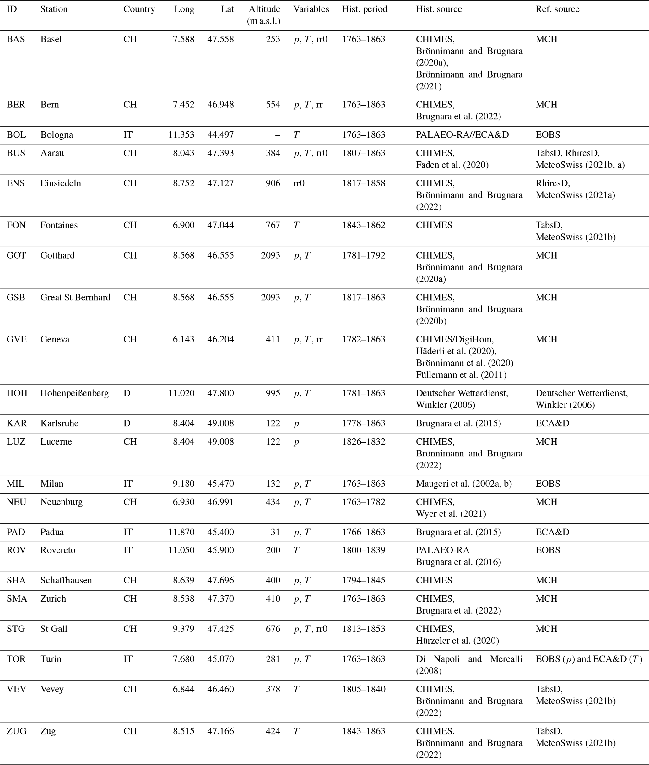
Table 2Stations used for independent evaluation of the 1763 to 1863 period from CHIMES. A description of the CHIMES data set and where it is available is found in Brugnara et al. (2020b). If additional evaluation of the station exists, the respective reference is noted under “Hist. sources”.

2.2 Present-day instrumental data
For every historical time series, the analogue selection requires an equivalent series in the reference period from 1961 to 2020. The long historical time series in Switzerland are mainly found in large cities. These locations also have a measurement station in the Swiss National Basic Climate Network (NBCN) (Füllemann et al., 2011; Begert et al., 2007). Precipitation and temperature time series from this network are quality controlled and homogenized by the Swiss Meteorological Service (Begert et al., 2005). For locations in Switzerland, where no data from the NBCN are available, we extracted the closest grid point from the daily temperature and precipitation fields (TabsD and RhiresD; for details about data sets, see the next section), and for sea level pressure we used the European EOBS data set v23.1 (Cornes et al., 2018). For time series in Germany and Italy, we used daily ECA&D station data (Klein Tank et al., 2002) if available or also the closest grid points from EOBS. To create time series of precipitation occurrences in the reference period, we used individual thresholds between 0.1 and 1 mm for each series for a rainy day. This is needed since the historical time series differ in how a wet day has been written down. To be able to use the full reference period as an analogue pool, all series in the reference period were gap filled by applying quantile mapping between the gridded data set (mainly EOBS) and the non-missing data of the time series. This bias correction is needed because a grid cell does not capture the local characteristics of a station and may thus have systematic biases. We choose empirical quantile mapping that estimates empirical cumulative distribution functions for the grid cell and station time series for 99 percentiles with a linear interpolation between the percentiles (Gudmundsson et al., 2012). The quantile mapping was calculated for every day of the year individually, including ±15 d around the target day because the biases between the grid and stations showed an annual cycle. The same approach was used to extend the station data up to 2020 or back to 1961 if they did not cover the full period from 1961 to 2020. Further, if it had not been done yet, we homogenized the series with the closest homogenized NBCN stations as a reference using the penalized maximal t test (Wang et al., 2007) and the penalized maximal F test (Wang, 2008) as implemented in Wang and Feng (2013) for break point detection. Table 1 summarizes the information on the reference stations.
2.3 Gridded data sets
The analogue fields are resampled from the two daily spatial data sets from MeteoSwiss for temperature (TabsD) and precipitation (RhiresD) (MeteoSwiss, 2021b, a). These data sets are available for the period from 1 January 1961 to 31 December 2020 at a resolution of 1×1 km. The temperature fields represent the free-air temperature at 2 m above ground and are interpolated from approximately 90 homogeneous long-term station series with a deterministic analysis method using nonlinear vertical temperature profiles and non-Euclidean distance (Frei, 2014). The precipitation fields cover all hydrological catchments that drain to locations within the Swiss border (MeteoSwiss, 2021a), i.e. also areas outside Switzerland. For the reconstruction, we only use the area that is covered during the entire 60 years excluding catchments to the south of Valais. The precipitation fields are generated using around 650 rain-gauge measurements within Switzerland and from neighbouring countries. They are based on the spatially interpolated monthly mean precipitation of a given day and spatial interpolations of relative anomalies (MeteoSwiss, 2021a).
2.4 Additional data sets
We want to restrict the selection of analogue days to days of similar weather. Therefore, we used a reconstruction of daily weather types covering the period of 1763 to 2009 from Schwander et al. (2017). This reconstruction is based on instrumental station records across Europe and the weather type classification by Weusthoff (2011). The weather type reconstruction also contains probabilities of the weather types for each day to account for the uncertainty in the reconstruction. For the period after 2009, we used the weather types provided by MeteoSwiss (Weusthoff, 2011).
The pre-processing steps of the gridded fields and observational data require additional reanalysis data. We use the palaeo-reanalysis EKF400v2 (Valler et al., 2022) for the homogenization of station data and for calculating a climatic offset between the reference period and the historical period to account for the warming since the pre-industrial period. This palaeo-reanalysis is based on atmosphere-only general circulation model simulations and assimilates a variety of data, such as early instrumental temperature and pressure data, documentary data, and tree-ring records. The reanalysis ERA5 (Hersbach et al., 2020) was used to remove temperature trends in the reference period (see Sect. 3.1).
In addition, we use the two monthly reconstructed gridded data sets for Switzerland, TrecabsM1864 and RrecabsM1864, which cover the period of 1864 to 2020 and which have been constructed with a focus on high temporal consistency (MeteoSwiss, 2021c).
For the analogue reconstruction, we mainly followed the approach implemented in Pfister et al. (2020). Some adaptations were necessary to reconstruct the early period from 1763 to 1863 because of the different network densities and different data types and because the data set extended further back in time. This adapted approach is described in the following sections. The period of 1864 to 1960 was reconstructed as in Pfister et al. (2020) with the exception that we removed the trend in the temperature data of the reference period (see Sect. 3.1), we changed the error covariance calculation of the observations for the assimilation procedure (see Sect. 3.3), and we implemented a quantile mapping approach considering the annual cycle of the precipitation bias (see Sect. 3.4). Figure 2 shows all required steps for creating the final reconstruction, including the data preparation, the reconstruction, and the cross-validation.

Figure 2Schematic of temperature and precipitation reconstruction. Blue ellipses show input data. The necessary data preparation steps are listed below the input data. Blue rectangles show the final output data. Details on the individual steps are found in Sect. 3.
3.1 Pre-processing
Before the analogue selection, the observations had to be pre-processed to make the historical observations comparable to the observations in the reference period from 1961 to 2020. Firstly, we removed the trend for the temperature data (observations and grids) in the reference period to make it equally likely to choose days from warmer years of the 21st century as analogues. To remove a trend representing average climatic changes and not local climatic changes, we calculated a linear trend for the 2 m temperatures from the zonal mean of the ERA5 reanalysis covering the period of 1961 to 2020 centred on 1991. For each grid cell and station, the trend of the closest latitude was subtracted. Secondly, for the analogue selection and for the resampling in the historical period before the year 1864, we removed a climatic offset from the reference temperature observations and the grid because the temperature data are warmer in the reference period than in the historical period of 1763 to 1863. A monthly transient offset was calculated based on the difference between the zonal mean temperature of a 31-year window centred on the reconstructed year (e.g. from 1748 to 1778 for the year 1763) and the zonal mean temperature in the reference period of 1961 to 2003 considering land areas only. In this case, the reference period is shorter because the EKF400v2 reanalysis ends in 2003. This offset was then subtracted from the data in the reference period (grid and observation) for every reconstructed day. Further, the historical stations had to be homogeneous with respect to their reference station. We performed a simple homogenization by calculating monthly differences between the historical and the reference stations over the full available period with respect to the closest grid points of the respective variable from the reanalysis EKF400v2 (Valler et al., 2022). The resulting difference between these two series is subtracted from the historical series to adjust them to EKF400v2. Lastly, we removed the seasonal cycle of temperature by fitting the first two harmonics of the temperature time series for observations and grid cells using least squares (see Pfister et al., 2020, for the equation).
3.2 Analogue reconstruction
The ARM samples meteorological fields for a historical period from the most similar days in a reference period. The most similar days, called the analogue days, are the days with the smallest differences calculated between the observational data in the historical period and observational data in the reference period. Our historical period starts in 1763 and is limited at the lower end by the availability of reconstructed weather types (Schwander et al., 2017). The reference period covers the period of the two gridded data sets TabsD and RhiresD from 1961 to 2020. These gridded data are resampled to generate a first reconstruction based on the best analogue day. To ensure that only physically plausible analogue days were chosen, the analogue selection was constrained to days with a similar weather type and days within the same season. All weather types with a cumulative probability of 95 % for the target days were admitted to the analogue pool to account for the uncertainty in the weather type reconstruction. This means we added up the probabilities of the most likely weather types until they reached 95 % together. Weather type probabilities were lower for the early days of the reconstruction in the 18th and at the beginning of the 19th century. For individual days, probabilities were so low (e.g. for 1 March 1803) that all weather types were included in the analogue pool. But the days of the analogue pool were still constrained by the seasons. A season was defined based on a moving window of ±60 d centred on the target day.
To reconstruct fields before 1864, we also used daily weather notes transformed into binary values of precipitation occurrence. The distance metrics used to find the closest analogue days in Pfister et al. (2020), i.e. the root mean squared error (RMSE), can however not be applied to categorical data (i.e. precipitation occurrence). Instead, we used the Gower distance, which allows for distances to be calculated for different variable types, such as continuous and count data (Gower, 1971; Kuhn and Johnson, 2019). It is defined as the average of partial distances across the variables (Eq. 1):
The partial distances are calculated as a range-normalized Manhattan distance for the quantitative variables temperature, pressure, and precipitation sum. For the binary variable precipitation occurrence, the partial distances are calculated as follows. If xik=xjk, then the partial distance is dijk=0, and otherwise if xik is not equal to xjk, dijk=1. We used an unweighted Gower distance. Thus, the distance metric for precipitation occurrence was either minimal (0) or maximal (1), which increased the weight of precipitation occurrence in the selection of the closest analogue. A first reconstruction was then obtained by resampling the fields based on the analogue day with the closest distance. To update the newer period from 1864 to 1960, we used the RMSE as a distance measure because a lot more precipitation measurements were available (compared to the earlier period) and the RMSE penalizes large errors. Changing the distance measure within the reconstruction period could lead to inhomogeneities. However, evaluations with both measures showed that the differences between the measures are small and the differences caused by the network changes are much larger.
3.3 Data assimilation for temperature fields
In a next step, the resampled temperature fields were improved by assimilating the available temperature measurements using ensemble Kalman fitting. This is an offline data assimilation approach, where the analysis is not passed to the next time step; i.e. every time step is handled individually (Bhend et al., 2012; Valler et al., 2022). Data assimilation tries to find an optimal representation of the true atmospheric state between the best guess of an atmospheric field (our best analogue field) and the observations by minimizing a cost function (Franke et al., 2017). In the case of normally distributed errors, this cost function can be minimized with a Kalman filter. The best estimate of a true atmospheric state, the analysis xa, is given by Eq. (2):
where xb refers to the best estimate (the resampled analogue fields), Pb is the model error covariance matrix calculated from the 50 best analogues for each target day, H extracts the observations from the model space, and R is the observation error covariance matrix. The second part on the right-hand side of Eq. (2), PbHT(HPbHT+R), is referred to as the Kalman gain K. To account for a bias in the covariance analysis, we used the ensemble square root filter as proposed by Whitaker and Hamill (2002) and updated the ensemble mean and the anomaly from the ensemble mean, individually yielding the separate equations Eqs. (3) and (4).
The Kalman gain for the mean K and anomaly were then calculated as follows:
Often localization of the background error covariance matrix Pb is used in data assimilation to avoid spurious error covariance. Testing different types of distance-, altitude-, and correlation-adjusted localization as proposed by Devers et al. (2021) did not improve results in our rather small area. Therefore, we did not apply localization.
We estimated the observation error covariance assuming that there is a linear relationship with distance between the variance of the differences in neighbouring observations as proposed by Wartenburger et al. (2013). The error covariance was estimated individually for the three periods 1763 to 1863, 1864 to 1960, and 1961 to 2020. As was to be expected, errors in the last period of 1961 to 2020 were smaller, and thus the skill of the cross-validation was overestimated. Due to the few available measurements within Switzerland in the period of 1763 to 1863, we also assimilated the temperature data from Hohenpeißenberg, Turin, Milan, and Rovereto. To do this, the observations from the best analogue days of the stations outside Switzerland (and therefore outside our grid) were added to the background xb, and, subsequently, the H operator was adjusted and Pb was calculated including these observations. The observation errors for these stations outside Switzerland were calculated as described above. For the years after 1864, only stations with correlation values above 0.975 are used for assimilation (see named stations in Fig. 1d and e). Before assimilating the observations we removed a monthly bias calculated between the observation and the closest grid points from the observations because the observations are biased with respect to the model grid.
3.4 Quantile mapping for precipitation fields
Despite using the same grids, precipitation biases occurred in the analogue-based reconstruction because precipitation measurements are very scarce and unevenly distributed across the area, leading to systematic biases in areas with no precipitation observations. To correct for these biases, we apply empirical quantile mapping calibrated between the reconstruction in the reference period and the original data set (RhiresD) for every grid cell (Gudmundsson et al., 2012; Feigenwinter et al., 2018; Rajczak et al., 2016). Correction factors were estimated for the 1st to 99th percentile using a linear interpolation between the percentiles. A wet-day threshold was set to 0.1 mm. Because quantile mapping showed seasonal biases of up to 1 mm per day in southern Switzerland, when quantile mapping was estimated for the entire year, we calculated it in 15 d steps throughout the year based on a 91 d window centred on these 15 d. This yielded a total of 24 steps, which was a compromise between making a bias correction for every day of the year individually and making the bias correction only for the four seasons. Because the biases in the precipitation reconstruction changed considerably based on the station network, quantile mapping was computed for the different networks (see Fig. 1) and then applied to the historical reconstruction depending on what network the historical period corresponded to best. Note that Fig. 1 only shows three examples of networks for the period before 1864. Quantile mapping was conducted for six different set-ups based on the station combinations occurring most often.
3.5 Evaluation
To evaluate the skill of the reconstructions, we (1) performed a cross-validation in the reference period of 1961 to 2020 and (2) compared the reconstructed fields with time series in the early period that have not been used for the reconstruction. For the cross-validation, we reconstructed the temperature and precipitation fields for the reference period of 1961 to 2020. For every day, the best analogue days were calculated by leaving out ±5 d around the target day. The reconstructed fields were then compared to the original fields using five standard measures. We calculated the root mean squared error (RMSE), Pearson correlation, mean bias, and the mean squared error skill score (MSESS) on the de-seasonalized temperature anomalies. For the MSESS, we used climatology as a reference, which is 0 in the case of anomalies. For precipitation we used the Spearman correlation, RMSE, mean bias, and the Brier score (Wilks, 2011). We used the Brier score to evaluate how well the reconstruction assigns wet and dry days. Therefore, instead of probabilities, the Brier score was calculated for wet and dry days, using 0.1 mm as a threshold. The Brier score returns the percentage of days that are wrongly assigned to wet or dry days. To assess the temporal persistence of the reconstruction on the day-to-day timescales in more detail, we performed two additional analyses. For temperature, we calculated the autocorrelation at a 1–20 d lag for all networks and compared these values to the autocorrelation in the original grid TabsD. For precipitation, we used two persistence indices suggested by Moon et al. (2019) to assess the mean persistence characteristics of precipitation and compared these to the persistence calculated with the original RhiresD grid.
Because the station network changes heavily over time, we performed the cross-validation for the different network set-ups shown in Fig. 1. The evaluation is done individually for every grid cell, i.e. evaluating the reconstruction in time. For the network shown in Fig. 1c, we also compared the original and reconstructed grids area-wise by calculating the above-mentioned measures in space and for two different altitude levels from 0 to 1000 and from 1000 to 2000 m a.s.l. for an area in Central Switzerland between 7.4 and 9.1∘ E and 46.5 to 47.3∘ N. This gives insights into how well the spatial structure is reproduced. The final reconstruction is, however, run on all available data.
For an independent evaluation, we compare the reconstruction with station data from seven entirely independent temperature series in the period of 1763 to 1863 (see Table 2) based on the same measures as described above. The mean bias was not calculated for series with seasonality removed but for the absolute temperature series. At the location of Bern, the precipitation reconstruction was compared to an independent series based on the Brier score and to monthly wet-day frequencies of the observation and the closest grid cell of the reconstruction. Furthermore, we explore the representation of the long-term variability by comparing our reconstructions to other data sets covering the same or similar periods.
4.1 Cross-validation during reference period
Cross-validation results for de-seasonalized temperature anomalies using the network as in Fig. 1c (i.e. a dense network for the historical period) show correlation values between 0.67 and 0.99 and an average of 0.92 to 0.95 (Fig. 3a to e) for all seasons and the annual evaluation. All periods show a spatial pattern with the highest correlations in the Swiss Plateau, lower values in the Alpine region, and the lowest values in the Canton of Ticino. The winter months (December to February) show the lowest correlation values, especially in the Alpine region, followed by autumn (SON) and spring (MAM). These spatial and seasonal differences are also present in the RMSE and MSESS evaluation (Fig. 3f to o). RMSEs range between 0.45 and 3.82 ∘C, with an average of 1.04 to 1.59 ∘C for all time aggregations. In winter, the errors are largest in the very south and east of Switzerland and in the Jura. MSESS values range between 0.34 and 0.98. The lowest values are found in the valleys of the Ticino, especially around Lago Maggiore in winter and autumn. Mean biases range between −0.34 and +0.08 ∘C (Fig. 3p to t). In winter, pronounced cold biases are present in the Alpine region, southern Switzerland, and the Jura. This is also the case for autumn, but biases are smaller. In spring, the largest cold biases are mainly found in the Alps but not in the Ticino, whereas in summer, biases range only between −0.06 and +0.08 ∘C.

Figure 3Cross-validation results of a network of 32 stations as in Fig. 1c for temperature anomalies during 1961–2020 for the four seasons (DJF, MAM, JJA, SON) and annually. (a–e) Pearson correlation, (f–j) RMSE, (k–o) MSESS, and (p–t) mean bias.
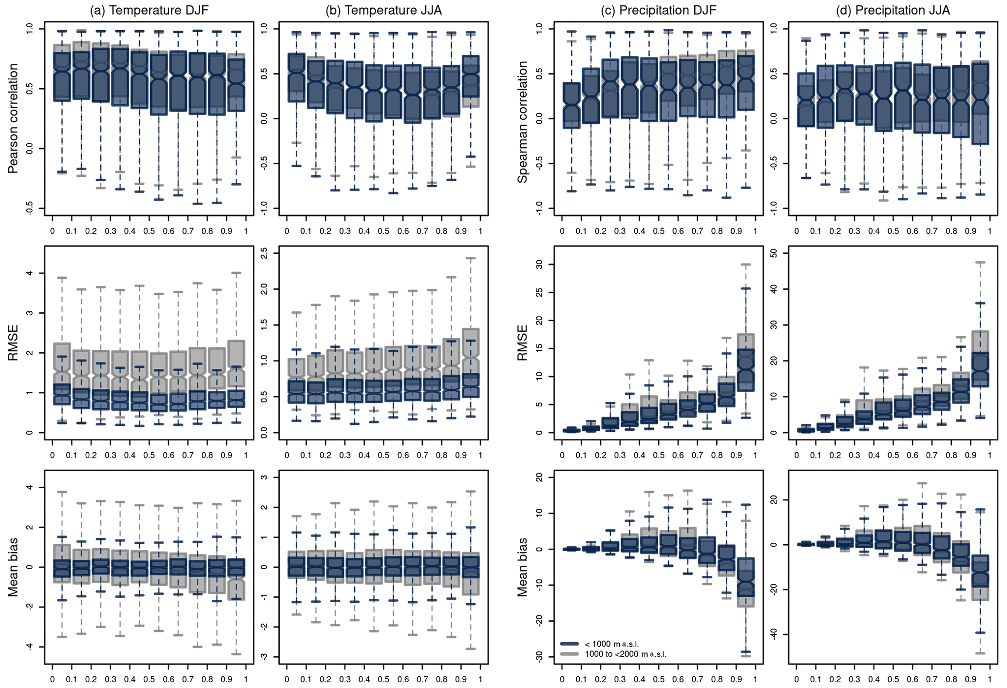
Figure 4Spatial evaluation of the reconstruction ordered according to the deciles of the area mean between 7.4 and 9.1∘ E and 46.5 to 47.3∘ N for the original data set. (a–b) DJF and JJA temperature evaluation with removed seasonality for Pearson correlation, RMSE, and mean bias. (c–d) DJF and JJA precipitation evaluation for Spearman correlation, RMSE, and mean bias. Blue values show all grid cells below 1000 m a.s.l.; grey values show grid cells above 1000 m a.s.l. The boxes range from the first to the third quartile, and whiskers extend to 1.5 times the interquartile range outside the box.
Spatial correlations do not show large differences in their performance with respect to the different deciles of the area mean for summer and winter and both altitude groups (Fig. 4a and b). In winter, RMSEs are larger for the coldest and the warmest days, while days in the middle of the distribution show lower errors. At altitudes above 1000 m a.s.l. in particular, the warmest days show larger RMSEs. In summer, cold days have low RMSEs, and the RMSEs increase with increasing temperatures. This effect is more pronounced for the higher-altitude group. The mean bias in the low-altitude group (below 1000 m a.s.l.) does not show differences in the deciles. However, for the higher-altitude group, the very cold days are too warm in the reconstruction and the very warm days are too cold. In summer, such an effect is not visible, but the spread of the mean bias distribution is generally larger for warm days than cold days.
Cross-validation results of the different networks, however, vary considerably. The network with only 11 measurements (Fig. 1a) has the lowest correlations, with values ranging between 0.58 and 0.99 for winter and 0.64 and 0.99 for summer (Fig. 5a and b). In the winter months in particular, this network performed worse with respect to correlation, RMSE, and MSESS. In summer, differences between networks are much smaller (Fig. 5b). The increase in observations in 1864 showed much better performance for all metrics; however, the change in the network from 41 observations to 108 did not lead to substantial improvements in the reconstructions. The spatial analyses of all five networks are shown in Fig. A1 in Appendix A for the annual evaluation.
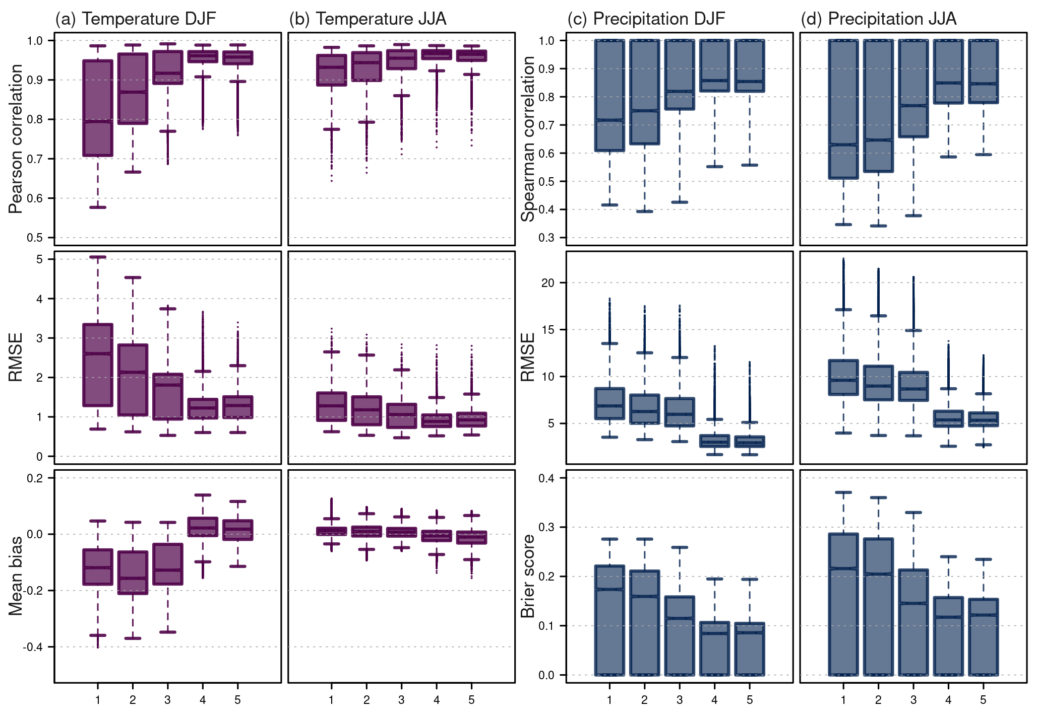
Figure 5Cross-validation results for the five networks shown in Fig. 1 for temperature anomalies during 1961–2020 (a) in winter (DJF) and (b) summer (JJA), showing Pearson correlation, RMSE, and mean bias, and for precipitation (c) in winter (DJF) and (d) summer (JJA), showing Spearman correlation, RMSE, and Brier score.
Further, the persistence of day-to-day temperature variability is slightly underestimated in the reconstructions compared to the original grid (Appendix, Fig. A3) with differences in the autocorrelations reaching up to 0.15 for the sparse networks. In the alpine areas in particular, autocorrelation at lags of up to 10 d is lower than in the original grid. This can be related to the network density and set-up. The sparser networks have lower autocorrelation values in the areas with very few observations.
These spatial and seasonal differences may be related to the sparse and unevenly distributed station network and the seasonal meteorological situations typical of Switzerland. In the winter half year (October to March) during calm flow situations, radiation fog and lifted fog (i.e. low stratus clouds) are a frequent phenomenon in the Swiss Plateau (Scherrer and Appenzeller, 2014). Such situations block direct radiation, leading to significantly lower temperatures below the cloud layer. Because temperature data were mainly available in the Swiss Plateau below this inversion layer, a day that is too cold for the Alpine area may be selected as an analogue day and the temperature assimilation may be too cold because the Alpine inversion layer is not well captured. An evaluation of fog days showed these large biases for the Alpine area (not shown). This is confirmed by the biases seen in Fig. 3k–o and would also lead to lower correlations and MSESS and larger RMSE. The overall better performance in summer compared to winter for all networks (Fig. 5a and b) can also be related to such badly captured inversion layers, which are not present in summer months. For a reconstruction of monthly temperature, Isotta et al. (2019) found that the magnitude of the warm anomalies in the areas above the inversion is not reproduced if only a few stations are available in the Alpine regions. For the network with only 11 stations (Fig. 1a), the temperature bias in winter is actually smaller compared to the network with 21 and 32 measurements (Fig. 1b and c). Networks 2 and 3 already contain the German station in Hohenpeißenberg at an altitude of 995 m a.s.l., and they also have more stations in the Swiss Plateau. An inversion layer captured wrongly because of the station distribution may also cause a larger bias.
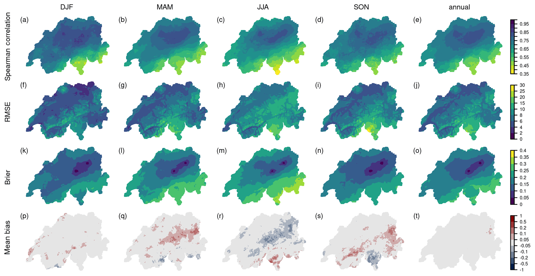
Figure 6Cross-validation results of a network of 31 stations as in Fig. 1c for precipitation during 1961–2020 for the four seasons (DJF, MAM, JJA, SON) and annually. (a–e) Spearman correlation, (f–j) RMSE, (k–o) Brier score, (p–t) mean bias. The RhiresD data set also contains the northern catchments in addition to Switzerland.
The cross-validation of the precipitation reconstruction shows a lower performance compared to de-seasonalized temperature (Figs. 5 and 6). Spearman correlations range between 0.39 and almost 1 for all seasons and the annual evaluation considering the network with 32 measurements (Fig. 5c). The Alpine region does not stand out in as pronounced a way as for the temperature validation. However, southern Switzerland, the Ticino, and the southern Grison valleys do have correlation values of only 0.35. In contrast with temperature, correlations are generally higher for winter than for summer months. RMSE ranges between 3.09 and 26.89 and is highest during the summer months in the Ticino. The Brier score is close to 0 around the locations where precipitation occurrence is registered and decreases with distance. As for the other metrics, especially in the summer months, the southern Ticino and southern Grison have very low values. The mean bias in all seasons is close to 0 because we conducted quantile mapping taking into account the annual cycle of precipitation differences between the reconstruction and the original data set (Fig. 5p to t).
With respect to the intensity of events in winter, days with more precipitation on an area-wide basis show higher correlations than days with less precipitation (Fig. 4c). In summer, spatial correlations do not vary in the median with respect to the area average intensity; however, the spread of the correlation increases for days with higher total precipitation. As is to be expected, the RMSE increases with increasing intensity of a rainy day. In summer in particular the RMSE can reach very high values for the strongest events. For higher altitudes, the values are even larger. These high values come from an underestimation of the strong precipitation events in both winter and summer, which is shown in Fig. 4c and d. Despite the bias correction, extreme precipitation is underestimated in the reconstruction by a median of up to 10 mm.
Differences between the networks are substantial for summer and winter (Fig. 5c and d), but the performance is generally better in winter than in summer. The sparsest network has a median correlation of 0.68, which increases considerably when stations are added. For the two networks after 1864, however, no more substantial changes occur. RMSEs are between 3.09 and 29.45 mm for the three networks of the early period and between 1.72 and 12.74 mm afterwards in winter. For the summer season, they are almost twice as large. For the annual evaluation of precipitation, the spatial analyses of all networks are shown in Fig. A2 in Appendix A.
Also, the persistence of dry and wet spells is underestimated in the reconstructions, although only slightly and with regional differences (Appendix Fig. A4). The fraction of dry (wet) days followed by dry (wet) days is up to 0.14 smaller in the reconstruction compared to the original data. The underestimation of the wet-day persistence is largest in the Ticino and for the sparse networks, indicating that wet spells are less well captured. For the dry-day persistence, no spatial pattern is visible. A lower persistence for both wet and dry days in the reconstruction can be expected since the analogue resampling does not consider temporal information.
The lower performance of the precipitation reconstruction can be expected, since precipitation is a much more heterogeneous variable than temperature on a daily timescale, impeding daily reconstruction, especially when only very few precipitation data are available. The performance differences in the reconstruction between winter and summer can be related to the type of precipitation occurring in these seasons. In summer, precipitation can be convective and very local, while in winter, precipitation is often stratiform, covering larger areas. This stratiform precipitation is easier to reconstruct. The Brier score decreases faster around the stations in summer than in winter. The poor performance with large RMSEs in the Ticino and the south-eastern Grison valley may come from convective or orographic precipitation not being captured at all in the precipitation data covering only northern Switzerland. But intense precipitation events are also difficult to capture in northern Switzerland (Fig. 4c and d). In contrast with Pfister et al. (2020), the mean bias of the uppermost percentile (Fig. 4c and d, lowest row) is on average negative; i.e. the reconstructed values are too low compared to the original. This may be because very few precipitation measurements enter the reconstruction, and thus days with high precipitation are not selected from the analogue pool.
The cross-validation results give us an impression of the performance of our reconstruction. However, they have some limitations. The cross-validation was performed based on station data in the reference period. These measurement data have a much higher quality than what we know from early instrumental data (see Sect. 2.1). Further, our analogue pool covers the same period as our reconstruction period. Therefore, it covers the same longer-scale variabilities but not necessarily in the same way as they occur in the early period between 1763 and 1863. With respect to temperature, we calculated an offset in order to account for the climatic change between the 18th century and the late 20th and early 21th centuries. This offset is based on a state-of-the-art data set but may not be accurate for the small and topographically heterogeneous area of Switzerland, thus adding an additional source of errors to the reconstruction.
4.2 Evaluation with independent data
A comparison with independent observations allowed us to assess the performance of the reconstruction in the reconstructed period itself, but the quality of the observations has to be considered. Temperature observations with removed seasonality in Aarau, Fribourg, Herisau, and Tegerfelden show Pearson correlations mostly above 0.85 (Fig. 7a to d). Nufenen, Bellinzona, and Lucerne show considerably lower values. The same pattern is also seen for the MSESS. RMSEs range between 1 and 4 ∘C. Again, Aarau, Fribourg, Herisau, and Tegerfelden have the smallest errors. The mean bias based on absolute values is mostly between −2 and 2 ∘C for Fribourg, Herisau, and Tegerfelden. For Bellinzona, Lucerne, and Nufenen, the reconstruction shows colder values than the observations in all seasons.
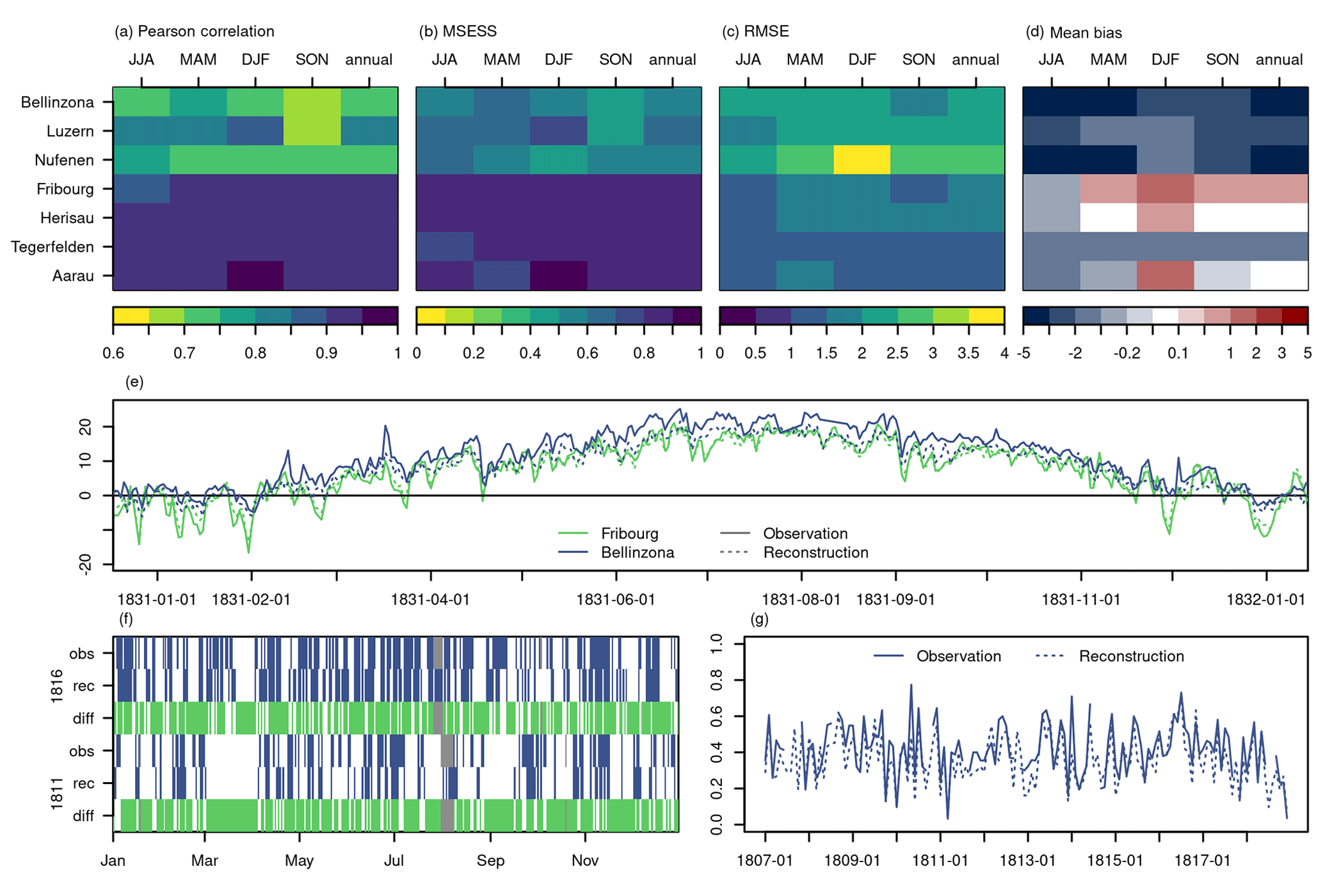
Figure 7Evaluation of the closest grid point from the reconstruction and the observations for values with removed seasonality. (a) Pearson correlation, (b) RMSE, (c) MSESS, and (d) mean bias. Each box shows the four seasons and annual values on the top x axis and the different locations on the y axis. Locations are marked with an asterisk in Fig. 1a. (e) Time series of two observations in Fribourg and Bellinzona and the closest grid points of the reconstruction for the year 1831. (f) Wet days for the observations from weather notes in Bern and reconstruction for the 2 years 1811 and 1816. A wet day is marked with a blue bar and a missing observation is marked with a grey bar. Green bars show the days that are correctly assigned to wet and dry. (g) Comparison of the monthly wet-day frequency for the period of 1807 to 1818 for the data from (f).
Fribourg, Herisau, Tegerfelden, and Aarau are all located in areas with a high station density (see Fig. 1). This contributes to the better performance of the reconstruction in these areas, but their good agreement confirms that for the Swiss Plateau our reconstruction provides useful results. Nufenen and Bellinzona show the lowest correlation values and the largest biases. For Bellinzona, Brönnimann and Brugnara (2022) showed that the subdaily measurements in July are considerably warmer than what is expected from the daily cycle representative of this area, most likely because of radiative biases. This would explain the fact that the reconstruction is colder than the observations, which is especially pronounced in summer (Fig. 7e). Furthermore, Bellinzona lies in an area with no nearby observations used in the reconstruction. Due to this, we would expect cold mean biases for winter as seen in the cross-validation but not for summer (Fig. 3). For Nufenen, the closest grid cell in the reconstruction corresponds to an altitude of 1866 m a.s.l., whereas the village Nufenen, where the measurements were taken, is at 1580 m a.s.l. An altitudinal difference of 300 m can explain the large negative biases found between observation and reconstruction.
For precipitation, a comparison with independent observations is only possible for a series of precipitation occurrence in Bern between 1807 and 1818. Based on the cross-validation, we can expect a Brier score of between 0.15 and 0.2 (i.e. up to 20 % of the days are wrongly assigned to a wet or dry day) for this location and the respective network. The Brier score between the closest grid cell in Bern and the precipitation occurrence series from weather notes yields 0.24 and is thus higher than the cross-validation results. However, we compare a station measurement with a grid cell (of 1×1 km) covering a slightly different scale. Also, precipitation occurrence may have a problem with accounting for nighttime precipitation correctly for the exact day of the weather notes. The gridded data are a daily sum between 06:00 in the morning and 06:00 the next day, while this may not be entirely clear for the weather notes. Figure 7f shows precipitation occurrence for a dry (1811) and a very wet year (1816). Long-lasting dry spells such as in March and April 1811 are captured by the reconstruction, as well as the overall wet summer of 1816, but for individual days, reconstructions deviate from observations. This is also seen in the comparison of the monthly wet-day frequency from the reconstruction and observation (Fig. 7g), which agree well overall (Pearson correlation of 0.84).
4.3 Assessment of long-term variability
The 258-year-long reconstructions should reproduce daily weather and long-term variability in temperature and precipitation over Switzerland. We assess this long-term variability by comparing the field mean of our data set to other data sets covering the same or similar periods (Valler et al., 2022; Casty et al., 2005; Brugnara et al., 2022; MeteoSwiss, 2021c). These data sets consist either of only observations, statistical reconstructions based on proxy data and observations, or reanalyses. The data sets are not independent from the Swiss reconstruction since they rely on the same or similar input data, and they are also not independent from each other. For details about the input data, refer to the references.
The annual temperature anomalies with respect to the 1871 to 1900 climatology agree well in all data sets for the reconstruction period from 1864 to 2020 (Fig. 8a). This period has good coverage of temperature data with high quality, and, thus, good agreement can be expected. Only the reconstruction by Casty et al. (2005) (hereafter referred to as Casty) is colder in the first half of the 20th century. Also, the data sets with a lower spatial resolution (EKF400v2, Casty) do not capture the steep warming at the end of the 20th century. Before 1864, deviations between the data sets are larger. The annual mean of the Swiss reconstruction is up to 0.5 ∘C warmer than EKF400v2 and the Swiss Plateau series before 1800. The temperature differences are larger in winter than in summer (not shown). There are several reasons this might lead to the warmer temperatures in the Swiss reconstruction. EKF400v2 is used for homogenization and for calculating an offset between the reference period and the historical period. This offset might be too small, especially in winter, since EKF400v2 is colder than the Swiss data in winter in the reference period.
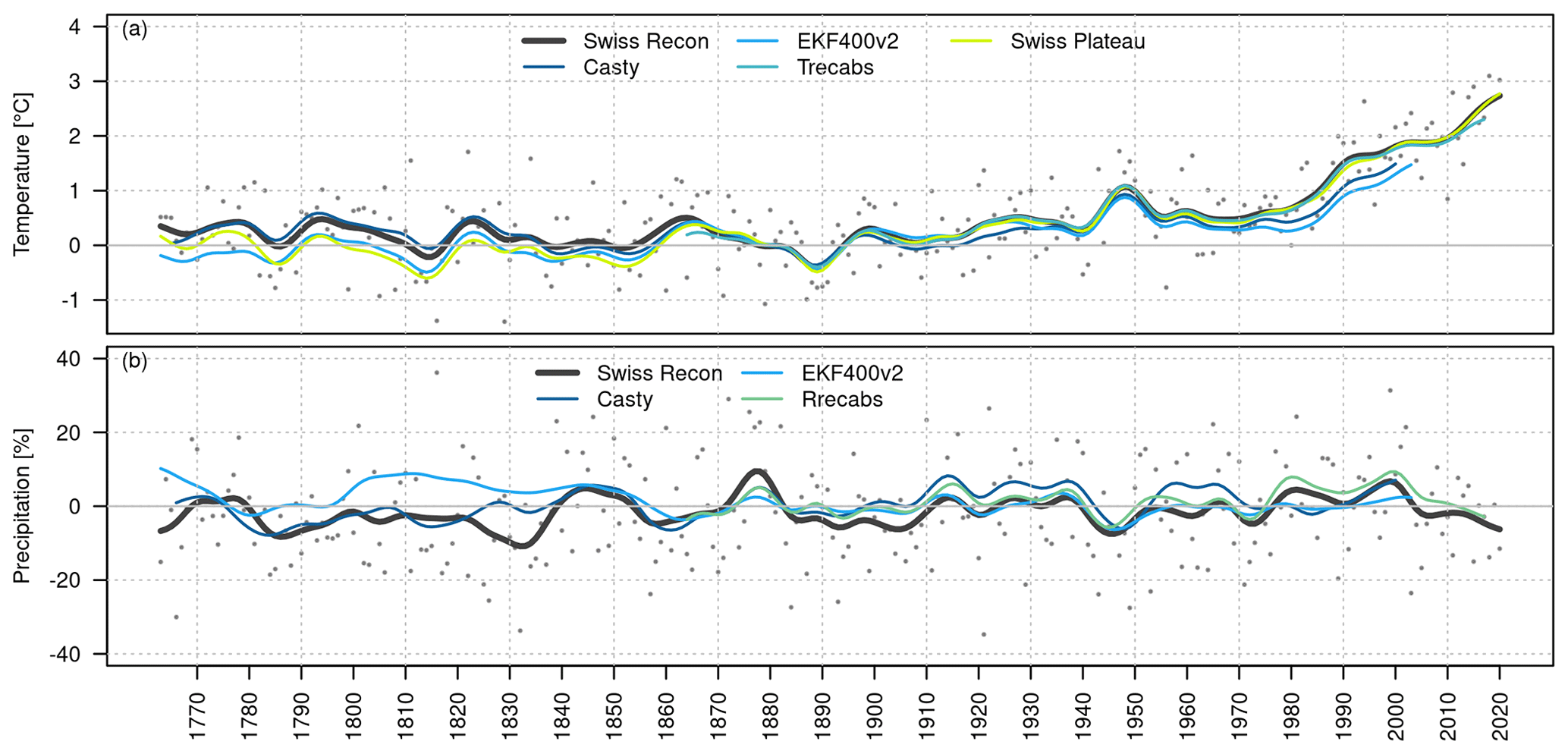
Figure 8(a) Long-term evolution of annual temperature anomalies in different data sets. (b) Long-term evolution of annual precipitation anomalies as a percentage deviation from the mean. The time series are smoothed with a Gaussian filter (σ= 3 years). Grey dots show reconstructed annual anomalies. All anomalies are calculated with respect to the 1871–1900 climatology for each data set. The time series either represent the field means (TrecabsM1864/RrecabsM1864, Swiss reconstruction) or the closest grid point of the data set. The Swiss Plateau time series is based on the Bern and Zurich series as described in Brugnara et al. (2022).
The agreement between precipitation reconstructions is much lower (Fig. 8b). After 1864, all data sets reproduce similar patterns but with different magnitudes. Differences in the anomalies reach up to 3 % when comparing our reconstruction to RrecabsM1864 (MeteoSwiss, 2021c). Before 1864, differences among the data sets are considerable. Whereas the reconstruction of Casty partly agrees in terms of the direction of the signal with the Swiss reconstruction, EKF400v2 does not agree at all. Also, the Swiss reconstruction is on average drier before 1864 compared to the period after 1864. The smoothed time series only shows periods (around 1770 and 1850) with wetter conditions than the average from 1871 to 1900. Since very little information on absolute precipitation enters the reconstruction and the bias correction might not fully correct the dry bias, too dry a reconstruction can be expected. However, individual years, such as 1816, the “year without a summer” (e.g. Luterbacher and Pfister, 2015), and the wet summer of 1770 (see next section), do show large positive precipitation anomalies (Figs. 8b and A5d). The precipitation reconstruction, therefore, needs to be used with care. Also, note that the main aim of the reconstruction was to create daily fields rather than creating a reconstruction with good long-term consistency. This needs to be considered when using the data set.
During the years 1770 to 1772 central Europe was hit by a severe famine which was considered one of the most devastating socio-ecological extreme events of the Little Ice Age. According to Collet (2018), the famine may have been of a similar magnitude to the famines of the 1315 to 1318 and 1570s, causing hundreds of thousands of deaths. The crisis was related to long-lasting wet and cold conditions between 1769 and 1772 from France to Ukraine and Switzerland to Scandinavia. It hit a society with low coping capacities and a very high cereal dependence beyond mere consumption; cereals were the key staple food but also served as a means of payment and taxation. This “cereal society” in Europe was highly vulnerable to adverse weather conditions, especially during the summer months. In the Czech Republic, around 10 % of the population died due to consecutive crop failures in the third year of the famine from 1771 to 1772 (Pfister and Brázdil, 2006). In contrast, for Switzerland, Pfister and Brázdil (2006) demonstrated that despite a loss of harvest, the famine was less severe due to a low social vulnerability by contemporary standards, effective interventions by the state, and the climate anomaly affecting only two harvests.
Collet (2018) summarized data from societal and natural archives describing the climate anomaly across Europe. According to him, the devastating impacts of the adverse weather were related to its length rather than its intensity. In fact, it has not been shown to be an outstanding climate anomaly with respect to magnitudes of temperature and precipitation anomalies in climate reconstructions (Luterbacher et al., 2004; PAGES2kConsortium, 2013; Pauling et al., 2006). A composite of 1769 to 1771 from the Old World Drought Atlas shows however very wet conditions mainly for a limited area of south-eastern Germany, northern Austria, and the western Czech Republic (Cook et al., 2015).
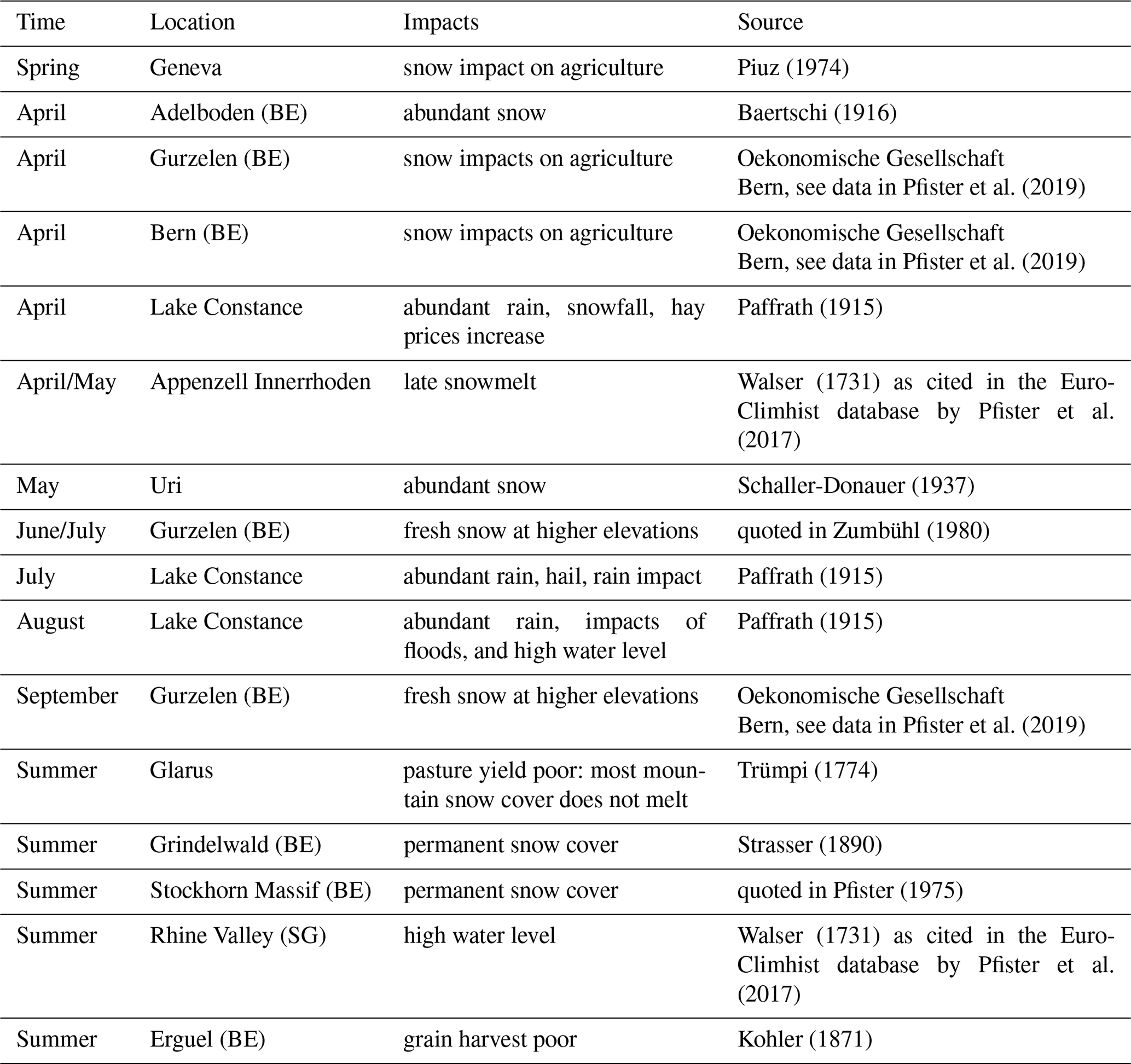
For Switzerland, we summarized documentary sources that reported the wet and cold weather conditions and related impacts for the summer half year of 1770 (Table 3). These reports include, for example, late snowfall, continuous snow cover, rain and flood impacts, and poor harvests. With our reconstructed daily fields, we tried to confirm the long-lasting wet and cold conditions described. However, the lack of precipitation observations in the reconstruction in particular has to be kept in mind.
Piuz (1974)Baertschi (1916)Pfister et al. (2019)Pfister et al. (2019)Paffrath (1915)Walser (1731)Pfister et al. (2017)Schaller-Donauer (1937)Zumbühl (1980)Paffrath (1915)Paffrath (1915)Pfister et al. (2019)Trümpi (1774)Strasser (1890)Pfister (1975)Walser (1731)Pfister et al. (2017)Kohler (1871)Table 3Selection of registered weather impacts from the wet and cold weather in Switzerland in the summer half year of 1770 based on our own sources (Brugnara et al., 2020b) and Euro-Climhist (Pfister et al., 2017). BE: Canton of Bern; SG: Canton of St Gall.
The area mean of the Swiss reconstruction does indeed show monthly precipitation anomalies (with respect to the 1763 to 1812 climatology) which are constantly above average for a period from 1769 to the end of 1771 (Fig. 9a). Two other data sets, EKF400v2 (Valler et al., 2022) and Casty (Casty et al., 2005), show peaks in 1770 and 1771 but not the persistent positive precipitation anomalies. Note that we use a 12-month running mean for the time series shown and that we select the closest grid cells in EKF400v2 and Casty. Thus, the data are not representative of exactly the same area. Temperature anomalies are negative especially for the first half year of 1770 but also for the beginning of 1771 (Fig. 9b). For temperature, the three data sets agree well, which is not the case for precipitation. For precipitation, however, the data sets agree better starting in the 19th century (not shown).
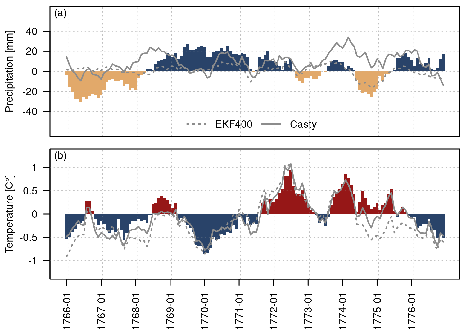
Figure 9(a) Area mean of monthly precipitation anomalies with respect to the monthly 1763 to 1812 means for the precipitation reconstruction (coloured bars); lines show the closest grid point of EKF400v2 (dashed) and of the reconstruction from Casty (solid). (b) Area mean of monthly temperature anomalies with respect to 1763 to 1812 for the temperature reconstruction; lines show the closest grid point of EKF400v2 (dashed) and the reconstruction from Casty (solid). All values are a mean over a 12-month window.
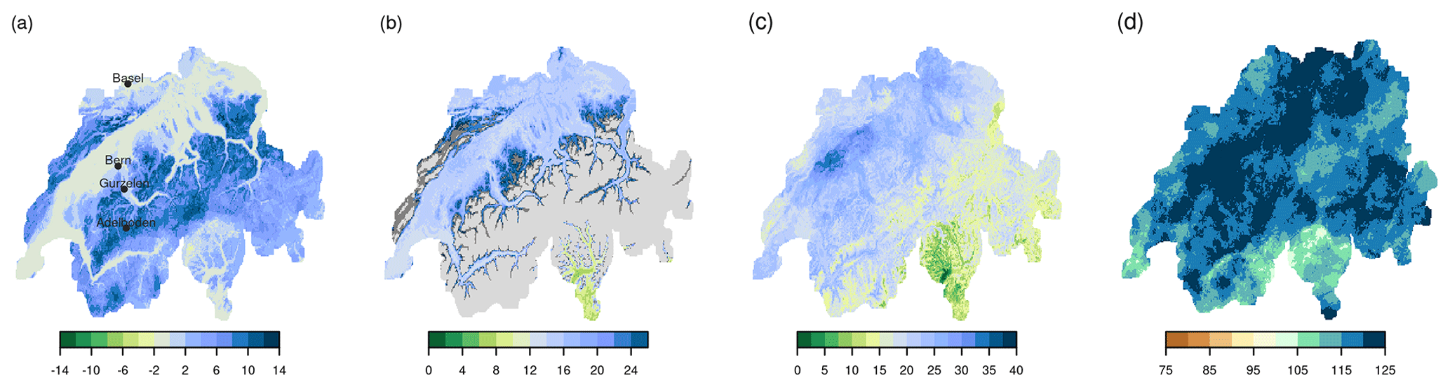
Figure 10(a) Anomaly of the number of days with snowfall for April 1770. Black dots denote areas where abundant snowfall was reported in historical sources. (b) Anomaly in days for the year 1770 when the threshold of 1000 GDDs was reached. Light-grey areas denote values where no climatology of a 1000 GDD threshold was calculated because the threshold was reached in less than 75 % of the years between 1763 and 1812. Dark grey denotes areas where the threshold of 1000 GDDs was not reached in the year 1770. (c) Anomaly of the number of cold days (days below the 20th percentile of daily mean temperature) for April to September 1770. (d) Wet-day anomaly in percentage for April to September 1770. All anomalies are calculated with respect to the 1763 to 1812 climatology.
Crop failure mainly relates to adverse weather conditions during the growing seasons. To track these adverse weather conditions, we exemplarily have a look at the summer half year of 1770. Several sources report abundant snowfall for the month of April 1770 (Table 3), which may have delayed the start of the growing season. Days with snowfall were calculated using a threshold of 2 ∘C for daily mean temperature and 1 mm for precipitation as it has been derived by Zubler et al. (2014). Optimal temperature thresholds for distinguishing snow from rain, however, depend heavily on the relative humidity of the air, which we do not have as a parameter for the historical time period, and they depend on the season (Jennings et al., 2018; Kienzle, 2008). Large parts of Switzerland show an above-average number of days with snowfall with respect to the 1763 to 1812 April climatology (Fig. 10a). In the pre-Alps and the Jura, up to 12 d more snowfall occurred than on average. For the surrounding hills of Bern and Gurzelen, for which historical sources reported snowfall, up to 3 snowfall days more occurred than usual, which, in relative terms, is almost a doubling with respect to the April climatology. In lower-elevation areas in the Swiss Plateau, low-elevation mountain valleys, and the Ticino, no snow days were registered in the reconstruction. For example, for Basel, weather notes by d'Annone (Brönnimann and Brugnara, 2020a) note snowfall for 4 d, but from our reconstruction no snowfall can be inferred. However, using daily data for snow detection is difficult, as the threshold for snow to occur may be reached at some point during the day, whereas it is not reached based on the daily mean; this is particularly the case in spring. Indeed, daily temperature values in Basel by d'Annone never reached values below 2.5 ∘C. However, the early morning measurements, for example, reached 1.6 and 1.9 ∘C on the days when snowfall was reported.
Crops require a certain amount of accumulated heat to reach their different phenological stages. The growing degree day (GDD) index can be used to express the heat accumulation needed until a phenological stage is reached (Wypych et al., 2017). The index is calculated as the sum of daily mean temperature above a certain threshold of daily mean temperature (e.g. Bonhomme, 2000). Here, we set this threshold to 5 ∘C. At a GDD of 1000 ∘C, various cereals, such as oat, barley, and wheat, reach their seed-filling phase (Miller et al., 2001). In the summer of 1770, a GDD of 1000 ∘C was reached around 15 d later in the Swiss Plateau than what would be expected on average for the period from 1763 to 1812. For higher-altitude locations, it was even reached up to 30 d later. This growth stage was therefore delayed by around half a month in the year 1770 (Fig. 10a). However, the weather conditions at later stages are also relevant for plant development and harvest. In the summer half year of 1770, the number of cold days was increased, which can be seen in the anomaly of a cold-day index, i.e. the number of days below the 20th quantile calculated for each day of the year. It shows above-average cold days ranging from +5 to +30 d (Fig. 10b) mainly for the area north of the Alps. In southern Switzerland, this was less pronounced, and only between 0 and 10 more cold days were registered.
Historical sources also reported wet conditions throughout the summer, for example for Lake Constance and the Rhine Valley (see Table 3, Paffrath, 1915 and Walser, 1731). For the summer season from April to September 1770, in most of northern Switzerland above-average wet days were recorded, with areas reaching up to 125 % wet days compared to the climatology of 1763 to 1812 (Fig. 10c). In the very south of southern Switzerland an above-average number of wet days was also recorded, although some areas also show an around average number of wet days. These values thus confirm the reports of wetter than usual weather.
However, if we compare the summer of 1770 to the summer of 1816 in our reconstruction, which is known as the year without a summer because of its very wet and cold conditions (Flückiger et al., 2017; Luterbacher and Pfister, 2015), these anomalies become small (see Appendix, Fig. A5). In 1816, a GDD of 1000 was reached in the Swiss Plateau on average 20 to 25 d later. The area where a GDD of 1000 is never reached is much larger, meaning that some cereals never fully developed. Up to 50 more cold days were registered during the summer of 1816, and wet days increased to up to 150 % compared to the 1763 to 1812 climatology. The summer of 1816 was, therefore, considerably more extreme. Our reconstruction might also be more accurate for the summer of 1816, particularly for precipitation, as up to four precipitation/precipitation occurrence time series, and also considerably more temperature measurements, were available in 1816.
With the reconstruction, we are nevertheless able to reproduce the wet and cold weather during 1769 to 1771 in Switzerland, which caused severe famines in parts of central Europe. Studies showed that, based on such gridded data sets, crop yields (Flückiger et al., 2017), for example, can be simulated. Such follow-up studies could also be applied to quantitatively reproduce crop losses for this famine for Switzerland based on the reconstruction presented here or even for the all of Europe.
In this study, we present a reconstruction of 258 years of high-resolution daily temperature and precipitation fields for Switzerland covering the period of 1763 to 2020. The data set is available in the open-access repository PANGAEA (https://doi.org/10.1594/PANGAEA.950236, Imfeld et al., 2022). Meteorological fields were resampled based on the most similar days in a reference period calculated from station measurements. The resampled temperature fields were further improved with data assimilation, and the resampled precipitation fields were bias corrected with quantile mapping. Extending a daily reconstruction for Switzerland as far back as the end of the 18th century was possible because of the data rescue efforts of CHIMES and follow-up projects (Brugnara et al., 2020b; Pfister et al., 2019; Brugnara et al., 2022).
Despite the considerable decrease in observations before 1864, the reconstruction still shows good results. Pearson correlations from a cross-validation of de-seasonalized temperature are between 0.58 and 0.99 and RMSEs are as high as 5 ∘C, including the very sparse network set-ups. Because very few or no station observations are available for the Alps and the south side of the Alps, the performance is considerably reduced in these regions. Cross-validation results for precipitation show lower performance than for temperature because few precipitation data were available and because precipitation is highly heterogeneous in space. The use of weather notes transformed to precipitation occurrence, however, increased the Spearman correlation and Brier score, especially around the measurement locations, but the good skills decreased rapidly with increasing distance from the observations.
The validation with independent station data confirmed the better reconstruction skills for temperature for stations in the Plateau region and worse results for stations in the Alps. A comparison with an independent time series of precipitation occurrence showed that around 76 % of the days are assigned to wet or dry days correctly and that the reconstruction was able to reproduce the monthly wet-day frequencies, indicating that the few observations of precipitation occurrence helped to reconstruct the monthly signal.
However, several limitations have to be considered when working with the data set. The results of the cross-validation cannot be used directly to infer the reconstruction skill in the historical period because the data quality differs and data gaps in the historical period have not been filled. Early instrumental data are a valuable source of information on daily weather in the 17th, 18th, and 19th centuries, but they come with uncertainties that are often hard to correct. A reconstruction based on such data inherits these errors and uncertainties. Also, the method assumes that our analogue pool represents the weather of the previous 200 years, but the 60 years of our analogue pool may not cover enough extreme events, which we are thus not able to reconstruct. Furthermore, the lack of stations south of the Alps and in the Alps considerably lowers the reconstruction quality in these areas. Reconstruction errors were large in the south of Switzerland especially for precipitation because the Alps act as a climatological barrier. Measurements would be needed to create a valid reconstruction for this area. Lastly, the changes in the network introduce inhomogeneities that need to be considered when working with long-term data.
Nevertheless, our case study on the famine years 1769 to 1772 shows that the wet and cold weather described in various documentary sources is reproduced in the reconstruction. The summer of 1770 was, for example, wetter and cooler than average, but it did not by far reach the wet and cold conditions of the summer of 1816 in Switzerland. The new reconstruction also opens up options of studying similar events in more detail, for example by feeding the reconstructed fields into crop models or hydrological models.
Further improvements in the data set could be obtained by incorporating more and better-corrected data. In particular, the long time series such as they have been created for Bern, Basel, Geneva, and Zurich (Brugnara et al., 2022) are very valuable. The precipitation reconstruction could profit substantially if more weather notes were digitized, although the latter is very tedious work. Other reconstruction approaches have been and are being explored that could also contribute to improved reconstructions, for example machine learning techniques and data assimilation for precipitation as well as methods including temporal information in the reconstruction. Furthermore, for some applications, not only daily mean temperature but also minimum and maximum temperature, and sunshine duration are needed and could be reconstructed in a similar manner since gridded data for a reference period are available.
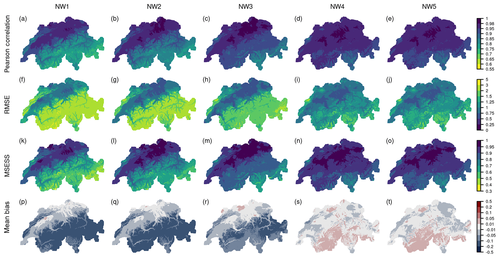
Figure A1Cross-validation results of all networks shown in Fig. 1a–e with 11, 21, 32, 43, and 108 time series used for reconstructing the precipitation fields. The cross-validation results are based on annual de-seasonalized temperature anomalies during 1961–2020. (a–e) Pearson correlation, (f–j) RMSE, (k–o) MSESS, and (p–t) mean bias.
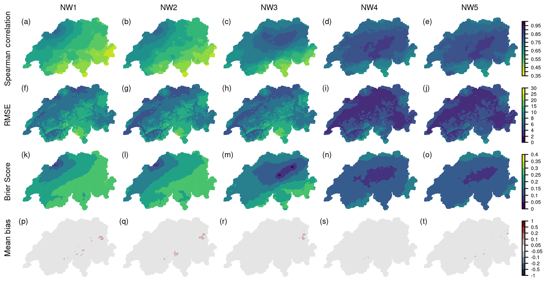
Figure A2Cross-validation results of all networks shown in Fig. 1a–e with 11, 21, 32, 43, and 108 time series used for reconstructing the precipitation fields. The cross-validation results are based on annual daily precipitation during 1961–2020. (a–e) Spearman correlation, (f–j) RMSE, (k–o) Brier score, and (p–t) mean bias. The RhiresD data set also contains the northern catchments that drain into Switzerland.
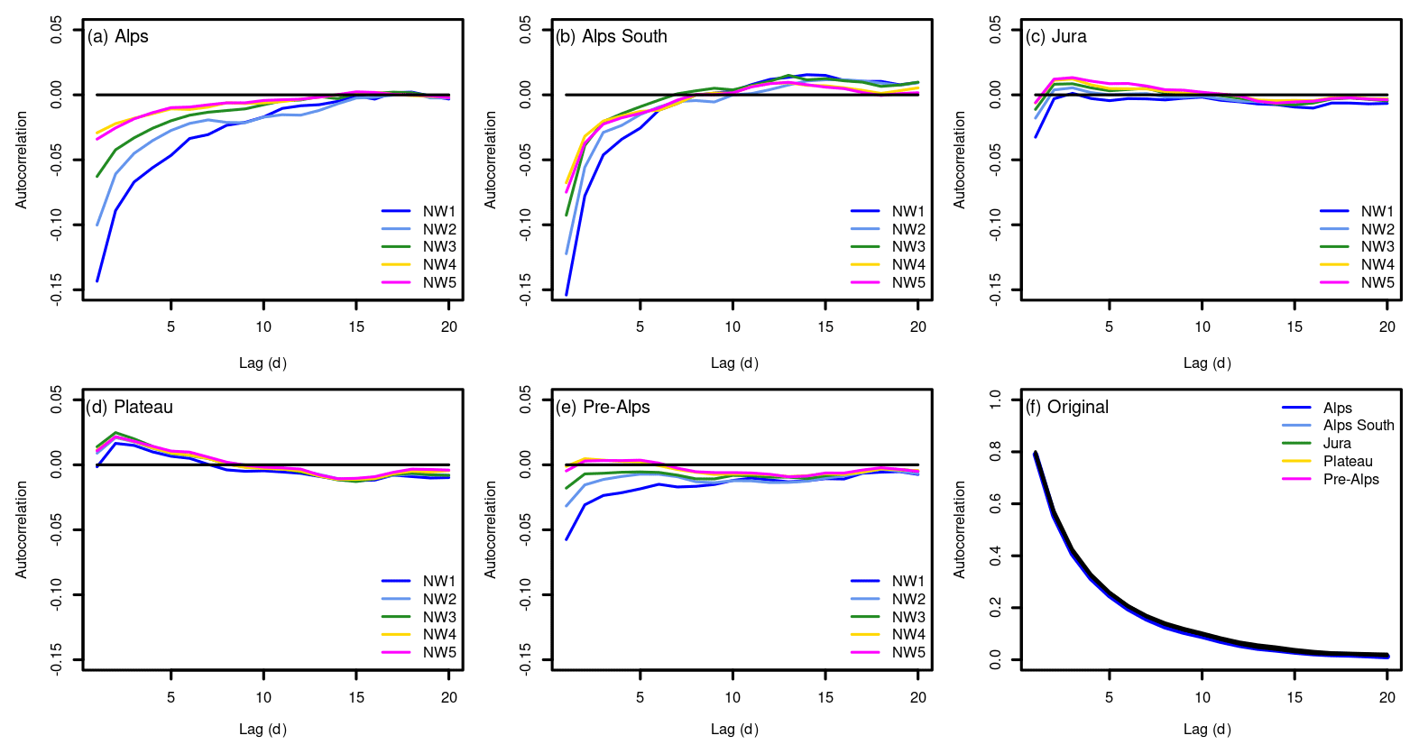
Figure A3(a–e) Differences between the area mean autocorrelation of the original grid and the reconstructed grid for the five different networks and for five regions of Switzerland. (f) Autocorrelation at lag day 1 to 20 for the original grid and for five regions covering Switzerland. The analysis is performed on the cross-validation results for the period of 1961 to 2020. See Fig. 1 for the network set-ups. The regions correspond to the major regions used for the national climate scenarios (NCCS, 2018).

Figure A4(a–e) Differences in the fraction of wet days followed by wet days for the cross-validations of the five networks (see Fig. 1) compared to the original data set (cross-validation minus original). (f–j) Same but for the fraction of dry days followed by dry days. A wet day is defined as a day above 0.1 mm. The fractions are calculated across the entire cross-validation period of 1961 to 2020.

Figure A5(a) Anomaly of the number of days with snowfall for April 1816. (b) Anomaly in days for the year 1816 when the threshold of 1000 GDDs was reached. Light-grey areas denote values where no climatology of a 1000 GDD threshold was calculated because the threshold was reached in less than 75 % of the years between 1763 and 1812. Dark grey denotes areas where the threshold of 1000 GDDs was not reached in the year 1816. (c) Anomaly of the number of cold days (days below the 20th percentile of daily mean temperature) for April to September 1816. (d) Wet-day anomaly in percentage for April to September 1816. For comparison with the summer of 1770, all anomalies are calculated with respect to the 1763 to 1812 climatology, which does not include the year 1816. Note that the colour scales are different from Fig. 10.
The code for the data preparation and the temperature and precipitation reconstruction is available in the Supplement.
Reconstructed daily precipitation and temperature data sets over the period 2 January 1763 to 31 December 2020 are published in the open-access repository PANGAEA https://doi.org/10.1594/PANGAEA.950236 (Imfeld et al., 2022). Station data used for the reconstruction are referenced in the sources in the article.
The supplement related to this article is available online at: https://doi.org/10.5194/cp-19-703-2023-supplement.
NI performed the reconstruction and the case studies and wrote the paper. LP created the first version of the data set for the period of 1864 to 2017. YB provided the historical observations. SB provided the idea for the reconstruction and supervised the process. LP, YB, and SB contributed to the paper.
The contact author has declared that none of the authors has any competing interests.
Publisher’s note: Copernicus Publications remains neutral with regard to jurisdictional claims in published maps and institutional affiliations.
This work was funded by the Swiss National Science Foundation (project “WeaR”, grant no. 188701) and by the European Commission through H2020 (ERC Grant PALAEO-RA 787574). The authors acknowledge the data provided by the projects CHIMES (SNF grant no. 169676) (Brugnara et al., 2020b), “Long Swiss Meteorological series” funded by MeteoSwiss through GCOS Switzerland (Brugnara et al., 2022), and DigiHom (Füllemann et al., 2011).
This work was funded by the Swiss National Science Foundation (project “WeaR”, grant no. 188701) and by the European Commission through H2020 (ERC Grant PALAEO-RA 787574).
This paper was edited by Hugues Goosse and reviewed by two anonymous referees.
Baertschi, A.: Wetterberichte einer Oberländischen Gemeinde vom 15.–19. Jahrhundert, in: Hardermannli, Illustrierte Sonntagsbeilage zum Oberländer Volksblatt, 16,, 1916. a
Begert, M., Schlegel, T., and Kirchhofer, W.: Homogeneous temperature and precipitation series of Switzerland from 1864 to 2000, Int. J. Climatol., 25, 65–80, https://doi.org/10.1002/joc.1118, 2005. a, b
Begert, M., Seiz, G., Foppa, N., Schlegel, T., Appenzeller, C., and Müller, G.: Die Überführung der klimatologischen Referenzstationen der Schweiz in das Swiss National Basic Climatological Network (Swiss NBCN), Arbeitsberichte der MeteoSchweiz, 215, https://www.meteoschweiz.admin.ch/dam/jcr:07db700e-0e10-4b75-b17a-39febbeb3fa1/arbeitsbericht215.pdf (last access: 23 March 2023), 2007. a
Bhend, J., Franke, J., Folini, D., Wild, M., and Brönnimann, S.: An ensemble-based approach to climate reconstructions, Clim. Past, 8, 963–976, https://doi.org/10.5194/cp-8-963-2012, 2012. a
Böhm, R., Jones, P. D., Hiebl, J., Frank, D., Brunetti, M., and Maugeri, M.: The early instrumental warm-bias: a solution for long central European temperature series 1760–2007, Climatic Change, 101, 41–67, https://doi.org/10.1007/s10584-009-9649-4, 2010. a, b
Bonhomme, R.: Bases and limits to using “degree. day” units, Eur. J. Agron., 13, 1–10, 2000. a
Brönnimann, S. (Ed.): Swiss Early Instrumental Meteorological Series, Geographica Bernensia G96, Bern, https://boris.unibe.ch/173023/1/G96.pdf (last access: 24 March 2023), 2020. a
Brönnimann, S.: From climate to weather reconstructions, PLOS Climate, 1, e0000034, https://doi.org/10.1371/journal.pclm.0000034, 2022. a
Brönnimann, S. and Brugnara, Y.: D'Annone's Meteorological Series from Basel, 1755–1804, Swiss Early Instrumental Meteorological Series, Bern: Geographica Bernensia, G96, 119–126, 2020a. a, b, c
Brönnimann, S. and Brugnara, Y.: The meteorological series from the Great St. Bernard, 1817–1863, Swiss Early Instrumental Meteorological Series, Bern: Geographica Bernensia, G96, 109–117, 2020b. a
Brönnimann, S. and Brugnara, Y.: Meteorological Series from Basel, 1825–1863, Swiss Early Instrumental Meteorological Series, Bern: Geographica Bernensia, G96, 127–138, 2021. a
Brönnimann, S. and Brugnara, Y.: Nineteenth century meteorological records from Vevey, Einsiedeln,Bellinzona, Lucerne, Fribourg, and Zug, Swiss Early Instrumental Meteorological Series, Bern: Geographica Bernensia, G96, 245–259, 2022. a, b, c, d, e, f, g, h
Brönnimann, S., Bühler, M., and Brugnara, Y.: The series from Geneva, 1799–1863, Swiss Early Instrumental Meteorological Series, Bern: Geographica Bernensia, G96, 47–59, 2020. a
Brugnara, Y.: Early Instrumental Temperature Records for Basel, Bern, Geneva, and Zurich, Bern Open Repository and Infor- mation System (BORIS) [data set], https://doi.org/10.48620/74, 2022. a
Brugnara, Y., Auchmann, R., Brönnimann, S., Allan, R. J., Auer, I., Barriendos, M., Bergström, H., Bhend, J., Brázdil, R., Compo, G. P., Cornes, R. C., Dominguez-Castro, F., van Engelen, A. F. V., Filipiak, J., Holopainen, J., Jourdain, S., Kunz, M., Luterbacher, J., Maugeri, M., Mercalli, L., Moberg, A., Mock, C. J., Pichard, G., Řezníčková, L., van der Schrier, G., Slonosky, V., Ustrnul, Z., Valente, M. A., Wypych, A., and Yin, X.: A collection of sub-daily pressure and temperature observations for the early instrumental period with a focus on the “year without a summer” 1816, Clim. Past, 11, 1027–1047, https://doi.org/10.5194/cp-11-1027-2015, 2015. a, b
Brugnara, Y., Auchmann, R., Brönnimann, S., Bozzo, A., Berro, D. C., and Mercalli, L.: Trends of mean and extreme temperature indices since 1874 at low-elevation sites in the southern Alps, J. Geophys. Res.-Atmos., 121, 3304–3325, https://doi.org/10.1002/2015JD024582, 2016. a
Brugnara, Y., Brönnimann, S., Zamuriano Carbajal, J. M., Schild, J., Rohr, C., and Segesser, D.: Reanalysis sheds lights on 1916 avalanche disaster, ECMWF Newsletter, 151, 28–34, https://doi.org/10.21957/h9b197, 2017. a, b
Brugnara, Y., Gilabert, A., Ventura, C., and Hunziker, S.: dataresqc: Quality control tools for climate data developed by the C3S Data Rescue Service, CRAN [code], https://cran.r-project.org/web/packages/dataresqc/index.html (last access: 23 March 2023), 2019. a
Brugnara, Y., Flückiger, J., and Brönnimann, S.: Instruments, procedures, processing, and analyses, Swiss Early Instrumental Meteorological Series, Bern: Geographica Bernensia, G96, 17–32, 2020a. a
Brugnara, Y., Pfister, L., Villiger, L., Rohr, C., Isotta, F. A., and Brönnimann, S.: Early instrumental meteorological observations in Switzerland: 1708–1873, Earth Syst. Sci. Data, 12, 1179–1190, https://doi.org/10.5194/essd-12-1179-2020, 2020b. a, b, c, d, e, f, g, h, i, j, k
Brugnara, Y., Hari, C., Pfister, L., Valler, V., and Brönnimann, S.: Pre-industrial temperature variability on the Swiss Plateau derived from the instrumental daily series of Bern and Zurich, Clim. Past, 18, 2357–2379, https://doi.org/10.5194/cp-18-2357-2022, 2022. a, b, c, d, e, f, g, h, i
Brönnimann, S., Allan, R., Ashcroft, L., Baer, S., Barriendos, M., Brázdil, R., Brugnara, Y., Brunet, M., Brunetti, M., Chimani, B., Cornes, R., Domínguez-Castro, F., Filipiak, J., Founda, D., Herrera, R. G., Gergis, J., Grab, S., Hannak, L., Huhtamaa, H., Jacobsen, K. S., Jones, P., Jourdain, S., Kiss, A., Lin, K. E., Lorrey, A., Lundstad, E., Luterbacher, J., Mauelshagen, F., Maugeri, M., Maughan, N., Moberg, A., Neukom, R., Nicholson, S., Noone, S., Øyvind Nordli, Ólafsdóttir, K. B., Pearce, P. R., Pfister, L., Pribyl, K., Przybylak, R., Pudmenzky, C., Rasol, D., Reichenbach, D., Řezníčková, L., Rodrigo, F. S., Rohr, C., Skrynyk, O., Slonosky, V., Thorne, P., Valente, M. A., Vaquero, J. M., Westcottt, N. E., Williamson, F., and Wyszyński, P.: Unlocking Pre-1850 Instrumental Meteorological Records: A Global Inventory, B. Am. Meteorol. Soc., 100, ES389–ES413, https://doi.org/10.1175/BAMS-D-19-0040.1, 2019. a
Caillouet, L., Vidal, J.-P., Sauquet, E., Graff, B., and Soubeyroux, J.-M.: SCOPE Climate: a 142-year daily high-resolution ensemble meteorological reconstruction dataset over France, Earth Syst. Sci. Data, 11, 241–260, https://doi.org/10.5194/essd-11-241-2019, 2019. a
Camuffo, D. and Jones, P.: Improved understanding of past climatic variability from early daily European instrumental sources, Springer Dordrecht, https://doi.org/10.1007/978-94-010-0371-1, 2002. a
Casty, C., Wanner, H., Luterbacher, J., Esper, J., and Böhm, R.: Temperature and precipitation variability in the European Alps since 1500, Int. J. Climatol., 25, 1855–1880, https://doi.org/10.1002/joc.1216, 2005. a, b, c, d
Casty, C., Raible, C. C., Stocker, T. F., Wanner, H., and Luterbacher, J.: A European pattern climatology 1766–2000, Clim. Dynam., 29, 791–805, https://doi.org/10.1007/s00382-007-0257-6, 2007. a
Collet, D.: Die doppelte Katastrophe: Klima und Kultur in der europäischen Hungerkrise 1770–1772, vol. 18 of Umwelt und Gesellschaft, Vandenhoeck & Ruprecht, https://doi.org/10.13109/9783666355929, 2018. a, b, c, d, e
Cook, E. R., Seager, R., Kushnir, Y., Briffa, K. R., Büntgen, U., Frank, D., Krusic, P. J., Tegel, W., van der Schrier, G., Andreu-Hayles, L., Baillie, M., Baittinger, C., Bleicher, N., Bonde, N., Brown, D., Carrer, M., Cooper, R., Čufar, K., Dittmar, C., Esper, J., Griggs, C., Gunnarson, B., Günther, B., Gutierrez, E., Haneca, K., Helama, S., Herzig, F., Heussner, K. U., Hofmann, J., Janda, P., Kontic, R., Köse, N., Kyncl, T., Levanč, T., Linderholm, H., Manning, S., Melvin, T.M., Miles, D., Neuwirth, B., Nicolussi, K., Nola, P., Panayotov, M., Popa, I., Rothe, A., Seftigen, K., Seim, A., Svarva, H., Svoboda, M., Thun, T., Timonen, M., Touchan, R., Trotsiuk, V., Trouet, V., Walder, F., Ważny, T., Wilson, R., and Zang, C.: Old World megadroughts and pluvials during the Common Era, Science Advances, 1, e1500561, https://doi.org/10.1126/sciadv.1500561, 2015. a
Cornes, R. C., van der Schrier, G., van den Besselaar, E. J., and Jones, P. D.: An ensemble version of the E-OBS temperature and precipitation data sets, J. Geophys. Res.-Atmos., 123, 9391–9409, https://doi.org/10.1029/2017JD028200, 2018. a
Devers, A., Vidal, J.-P., Lauvernet, C., and Vannier, O.: FYRE Climate: a high-resolution reanalysis of daily precipitation and temperature in France from 1871 to 2012, Clim. Past, 17, 1857–1879, https://doi.org/10.5194/cp-17-1857-2021, 2021. a, b
Di Napoli, G. and Mercalli, L.: Il clima di Torino: tre secoli di osservazioni meteorologiche, SMS – Società-Meteorologica Subalpin, Turin, Italy, 936 pp., ISBN 8890302348, 2008. a
Dobrovolnỳ, P., Moberg, A., Brázdil, R., Pfister, C., Glaser, R., Wilson, R., van Engelen, A., Limanówka, D., Kiss, A., Halíčková, M., Macková, J., Riemann, D., Luterbacher, J., and Böhm, R.: Monthly, seasonal and annual temperature reconstructions for Central Europe derived from documentary evidence and instrumental records since AD 1500, Climatic Change, 101, 69–107, https://doi.org/10.1007/s10584-009-9724-x, 2010. a
Estévez, J., Gavilán, P., and García-Marín, A.: Spatial regression test for ensuring temperature data quality in southern Spain, Theor. Appl. Climatol., 131, 309–318, https://doi.org/10.1007/s00704-016-1982-8, 2018. a
Faden, M., Villiger, L., Brugnara, Y., and Brönnimann, S.: The meteorological series from Aarau, 1807–1865, Swiss Early Instrumental Meteorological Series, Bern: Geographica Bernensia, G96, 61–72, 2020. a, b
Feigenwinter, I., Kotlarski, S., Casanueva, A., Schwierz, C., and Liniger, M.: Exploring quantile mapping as a tool to produce user-tailored climate scenarios for Switzerland, MeteoSchweiz, Technical Report, MeteoSwiss, 270, https://www.meteoswiss.admin.ch/dam/jcr:1b810050-11a2-415d-b439-3b2eb75f9693/MeteoSchweiz_Fachbericht_270_final.pdf (last access: 23 March 2023), 2018. a
Flückiger, S., Brönnimann, S., Holzkämper, A., Fuhrer, J., Krämer, D., Pfister, C., and Rohr, C.: Simulating crop yield losses in Switzerland for historical and present Tambora climate scenarios, Environ. Res. Lett., 12, 074026, https://doi.org/10.1088/1748-9326/aa7246, 2017. a, b, c, d
Franke, J., Brönnimann, S., Bhend, J., and Brugnara, Y.: A monthly global paleo-reanalysis of the atmosphere from 1600 to 2005 for studying past climatic variations, Scientific Data, 4, 1–19, https://doi.org/10.1038/sdata.2017.76, 2017. a
Frei, C.: Interpolation of temperature in a mountainous region using nonlinear profiles and non-Euclidean distances, Int. J. Climatol., 34, 1585–1605, https://doi.org/10.1002/joc.3786, 2014. a
Füllemann, C., Begert, M., Croci-Maspoli, M., and Bönnimann, S.: Digitalisieren und Homogenisieren von historischen Klimadaten des Swiss NBCN: Resultate aus DigiHom, Arbeitsberichte der MeteoSchweiz, 236, https://www.meteoswiss.admin.ch/dam/jcr:c0d90a48-a05d-4ac9-9cf3-10769270d75e/ab236.pdf (last access: 23 March 2023), 2011. a, b, c, d
Gómez-Navarro, J. J., Zorita, E., Raible, C. C., and Neukom, R.: Pseudo-proxy tests of the analogue method to reconstruct spatially resolved global temperature during the Common Era, Clim. Past, 13, 629–648, https://doi.org/10.5194/cp-13-629-2017, 2017. a
Gower, J. C.: A general coefficient of similarity and some of its properties, Biometrics, 27, 857–871, https://doi.org/10.2307/2528823, 1971. a
Gudmundsson, L., Bremnes, J. B., Haugen, J. E., and Engen-Skaugen, T.: Technical Note: Downscaling RCM precipitation to the station scale using statistical transformations – a comparison of methods, Hydrol. Earth Syst. Sci., 16, 3383–3390, https://doi.org/10.5194/hess-16-3383-2012, 2012. a, b
Häderli, S., Pfister, S. M., Villiger, L., Brugnara, Y., and Brönnimann, S.: Two meteorological series from Geneva, 1782–1791, Swiss Early Instrumental Meteorological Series, Bern: Geographica Bernensia, G96, 33–46, 2020. a
Hari, C., Brugnara, Y., Rohr, C., and Brönnimann, S.: Meteorological Observations in Bern and Vicinity, 1777-1834, Swiss Early Instrumental Meteorological Series, Bern: Geographica Bernensia, G96, 199–211, 2022. a
Harvey-Fishenden, A. and Macdonald, N.: Evaluating the utility of qualitative personal diaries in precipitation reconstruction in the eighteenth and nineteenth centuries, Clim. Past, 17, 133–149, https://doi.org/10.5194/cp-17-133-2021, 2021. a
Hersbach, H., Bell, B., Berrisford, P., Hirahara, S., Horányi, A., Muñoz-Sabater, J., Nicolas, J., Peubey, C., Radu, R., Schepers, D., Simmons, A., Soci, C., Abdalla, S., Abellan, X., Balsamo, G., Bechtold, P., Biavati, G., Bidlot, J., Bonavita, M., De Chiara, G., Dahlgren, P., Dee, D., Diamantakis, M., Dragani, R., Flemming, J., Forbes, R., Fuentes, M., Geer, A., Haimberger, L., Healy, S., Hogan, R. J., Hólm, E., Janisková, M., Keeley, S., Laloyaux, P., Lopez, P., Lupu, C., Radnoti, G., de Rosnay, P., Rozum, I., Vamborg, F., Villaume, S., and Thépaut, J. N.: The ERA5 global reanalysis, Q. J. Roy. Meteor. Soc., 146, 1999–2049, https://doi.org/10.1002/qj.3803, 2020. a
Hupfer, F.: Das Wetter der Nation: Meteorologie, Klimatologie und der schweizerische Bundesstaat, 1860–1914, Chronos Verlag, ISBN 978-3-0340-1502-8, 2019. a
Hürzeler, A., Brugnara, Y., and Brönnimann, S.: The meteorological record from St. Gall, 1812–1853, Swiss Early Instrumental Meteorological Series, Bern: Geographica Bernensia, G96, 87–95, 2020. a
Imfeld, N., Pfister, L., Brugnara, Y., and Brönnimann, S.: Daily high-resolution temperature and precipitation fields for Switzerland from 1763 to 2020, PANGAEA [data set], https://doi.org/10.1594/PANGAEA.950236, 2022. a, b, c
Isotta, F. A., Begert, M., and Frei, C.: Long-term consistent monthly temperature and precipitation grid data sets for Switzerland over the past 150 years, J. Geophys. Res.-Atmos., 124, 3783–3799, https://doi.org/10.1029/2018JD029910, 2019. a
Jennings, K. S., Winchell, T. S., Livneh, B., and Molotch, N. P.: Spatial variation of the rain–snow temperature threshold across the Northern Hemisphere, Nat. Commun., 9, 1–9, https://doi.org/10.1038/s41467-018-03629-7, 2018. a
Keller, V. D. J., Tanguy, M., Prosdocimi, I., Terry, J. A., Hitt, O., Cole, S. J., Fry, M., Morris, D. G., and Dixon, H.: CEH-GEAR: 1 km resolution daily and monthly areal rainfall estimates for the UK for hydrological and other applications, Earth Syst. Sci. Data, 7, 143–155, https://doi.org/10.5194/essd-7-143-2015, 2015. a
Kienzle, S. W.: A new temperature based method to separate rain and snow, Hydrol. Process., 22, 5067–5085, https://doi.org/10.1002/hyp.7131, 2008. a
Klein Tank, A., Wijngaard, J., Können, G., Böhm, R., Demarée, G., Gocheva, A., Mileta, M., Pashiardis, S., Hejkrlik, L., Kern-Hansen, C., Heino, R., Bessemoulin, P., Müller-Westermeier, G., Tzanakou, M., Szalai, S., Pálsdóttir, T., Fitzgerald, D., Rubin, S., Capaldo, M., Maugeri, M., Leitass, A., Bukantis, A., Aberfeld, R., van Engelen, A. F. V., Forland, E., Mietus, M., Coelho, F., Mares, C., Razuvaev, V., Nieplova, E., Cegnar, T., Antonio López, J., Dahlström, B., Moberg, A., Kirchhofer, W., Ceylan, A., Pachaliuk, O., Alexander, L. V., and Petrovic, P.: Daily dataset of 20th-century surface air temperature and precipitation series for the European Climate Assessment, Int. J. Climatol., 22, 1441–1453, https://doi.org/10.1002/joc.773, 2002. a, b
Kohler, X.: Observations Météorologiques, Économiques et Rurales dans l'Erguel et la Prévôté de Moutier de 1747 à 1804 par le pasteur T. Frêne, in: Actes de la Société Jurassienne d' Émulation, 22, 213–267, https://doi.org/10.5169/seals-684289, 1871. a
Kuhn, M. and Johnson, K.: Feature engineering and selection: A practical approach for predictive models, CRC Press, ISBN 978-1-13-807922-9, 2019. a
Luterbacher, J. and Pfister, C.: The year without a summer, Nat. Geosci., 8, 246–248, https://doi.org/10.1038/ngeo2404, 2015. a, b
Luterbacher, J., Dietrich, D., Xoplaki, E., Grosjean, M., and Wanner, H.: European Seasonal and Annual Temperature Variability, Trends, and Extremes Since 1500, Science, 303, 1499–1503, https://doi.org/10.1126/science.1093877, 2004. a, b
Maugeri, M., Buffoni, L., and Chlistovsky, F.: Daily Milan temperature and pressure series (1763–1998): history of the observations and data and metadata recovery, Clim. Change, 53, 101–117, https://doi.org/10.1007/978-94-010-0371-1_4, 2002a. a
Maugeri, M., Buffoni, L., Delmonte, B., and Fassina, A.: Daily Milan temperature and pressure series (1763–1998): completing and homogenising the data, Clim. Change, 53, 119–149, https://doi.org/10.1007/978-94-010-0371-1_5, 2002b. a
MeteoSwiss: Documentation of MeteoSwiss Grid-Data Products. Daily Precipitation (final analysis): RhiresD, https://www.meteoswiss.admin.ch/dam/jcr:4f51f0f1-0fe3-48b5-9de0-15666327e63c/ProdDoc_RhiresD.pdf (last access: 23 March 2023), 2021a. a, b, c, d, e
MeteoSwiss: Documentation of MeteoSwiss Grid-Data Products. Daily Mean, Minimum and Maximum Temperature: TabsD, TminD, TmaxD, https://www.meteoswiss.admin.ch/dam/jcr:818a4d17-cb0c-4e8b-92c6-1a1bdf5348b7/ProdDoc_TabsD.pdf (last access: 23 March 2023), 2021b. a, b, c, d, e
MeteoSwiss: Documentation of MeteoSwiss Grid-Data Products. Monthly Temperature and Precipitation Reconstructions, https://www.meteoschweiz.admin.ch/dam/jcr:98a965e5-30dd-4fdf-a42b-74c414a4a731/ProdDoc_rec.pdf (last access: 7 February 2023), 2021c. a, b, c
Miller, P., Lanier, W., and Brandt, S.: Using growing degree days to predict plant stages, Montguide MT200103 AG, https://landresources.montana.edu/soilfertility/documents/PDF/pub/GDDPlantStagesMT200103AG.pdf (last access: 23 March 2023), 2001. a
Moon, H., Gudmundsson, L., Guillod, B. P., Venugopal, V., and Seneviratne, S. I.: Intercomparison of daily precipitation persistence in multiple global observations and climate models, Environ. Res. Lett., 14, 105009, https://doi.org/10.1088/1748-9326/ab4169, 2019. a
Muñoz-Sabater, J., Dutra, E., Agustí-Panareda, A., Albergel, C., Arduini, G., Balsamo, G., Boussetta, S., Choulga, M., Harrigan, S., Hersbach, H., Martens, B., Miralles, D. G., Piles, M., Rodríguez-Fernández, N. J., Zsoter, E., Buontempo, C., and Thépaut, J.-N.: ERA5-Land: a state-of-the-art global reanalysis dataset for land applications, Earth Syst. Sci. Data, 13, 4349–4383, https://doi.org/10.5194/essd-13-4349-2021, 2021. a
Murphy, C., Wilby, R. L., Matthews, T., Horvath, C., Crampsie, A., Ludlow, F., Noone, S., Brannigan, J., Hannaford, J., McLeman, R., and Jobbova, E.: The forgotten drought of 1765–1768: Reconstructing and re-evaluating historical droughts in the British and Irish Isles, Int. J. Climatol., 40, 5329–5351, https://doi.org/10.1002/joc.6521, 2020. a
NCCS: Major regions, https://www.nccs.admin.ch/nccs/en/home/regions/grossregionen.html (last access: 23 March 2023), 2018. a
Paffrath, J.: Schriften des Vereins für die Geschichte des Bodensees und seiner Umgebung, chap. Zum Wetterverlauf am Bodensee, Kommissionsverlag von Joh. Thom. Stettner, Lindau, https://www.digishelf.de/objekt/bsz014854767_1915/172/LOG_0020/ (last access: 23 March 2023), 1915. a, b, c, d
PAGES2kConsortium: Continental-scale temperature variability during the past two millennia, Nat. Geosci., 6, 339–346, https://doi.org/10.1038/ngeo1797, 2013. a
Pappert, D., Barriendos, M., Brugnara, Y., Imfeld, N., Jourdain, S., Przybylak, R., Rohr, C., and Brönnimann, S.: Statistical reconstruction of daily temperature and sea level pressure in Europe for the severe winter 1788/89, Clim. Past, 18, 2545–2565, https://doi.org/10.5194/cp-18-2545-2022, 2022. a, b
Pauling, A., Luterbacher, J., Casty, C., and Wanner, H.: Five hundred years of gridded high-resolution precipitation reconstructions over Europe and the connection to large-scale circulation, Clim. Dynam., 26, 387–405, https://doi.org/10.1007/s00382-005-0090-8, 2006. a
Pfister, C.: Agrarkonjunktur und Witterungsverlauf im westlichen schweizer Mittelland zur Zeit der ökonomischen Patrioten, 1755–1797: ein Beitrag zur Umwelt-u. Wirtschaftsgeschichte des 18. Jahrhunderts, PhD Thesis, 2 Edn., Lang Druck AG, 1975. a
Pfister, C.: Das Klima der Schweiz von 1525-1860 und seine Bedeutung in der Geschichte von Bevölkerung und Landwirtschaft, 1 Edn., Haupt, ISBN 3258039569, 1988. a
Pfister, C. and Brázdil, R.: Social vulnerability to climate in the “Little Ice Age”: an example from Central Europe in the early 1770s, Clim. Past, 2, 115–129, https://doi.org/10.5194/cp-2-115-2006, 2006. a, b, c, d
Pfister, C. and Wanner, H.: Klima und Gesellschaft in Europa. Die letzten tausend Jahre, Haupt Verlag, ISBN 978-3-258-08182-3, 2021. a
Pfister, C., Rohr, C., and Jover, A. C. C.: Euro-Climhist: eine Datenplattform der Universität Bern zur Witterungs-, Klima-und Katastrophengeschichte, Wasser Energie Luft, Schweizerischer Wasserwirtschaftsverband, 109, 45–48, https://doi.org/10.7892/boris.97013, 2017. a, b, c
Pfister, L., Hupfer, F., Brugnara, Y., Munz, L., Villiger, L., Meyer, L., Schwander, M., Isotta, F. A., Rohr, C., and Brönnimann, S.: Early instrumental meteorological measurements in Switzerland, Clim. Past, 15, 1345–1361, https://doi.org/10.5194/cp-15-1345-2019, 2019. a, b, c, d, e, f
Pfister, L., Brönnimann, S., Schwander, M., Isotta, F. A., Horton, P., and Rohr, C.: Statistical reconstruction of daily precipitation and temperature fields in Switzerland back to 1864, Clim. Past, 16, 663–678, https://doi.org/10.5194/cp-16-663-2020, 2020. a, b, c, d, e, f, g, h, i, j, k
Piuz, A.-M.: Climat, récoltes et vie des hommes à Genève, XVIe-XVIIIe siècle, Ann. Hist. Sci. Soc., 29, 599–618, https://doi.org/10.3406/ahess.1974.293496, 1974. a
Rajczak, J., Kotlarski, S., and Schär, C.: Does quantile mapping of simulated precipitation correct for biases in transition probabilities and spell lengths?, J. Climate, 29, 1605–1615, https://doi.org/10.1175/JCLI-D-15-0162.1, 2016. a
Rössler, O. and Brönnimann, S.: The effect of the Tambora eruption on Swiss flood generation in 1816/1817, Sci. Total Environ., 627, 1218–1227, https://doi.org/10.1016/j.scitotenv.2018.01.254, 2018. a
Rutishauser, T., Brönnimann, S., Gehrig, R., Pietragalla, B., Baumgarten, F., Vitasse, Y., Stöckli, S., Pfister, C., Holzkämper, A., Hund, A., Fossati, D., Meier, M., Weingartner, R., and Buchmann, M.: Klimawandel und Jahreszeiten (Reihe G Grundlagenforschung G97), Geographica Bernensia, https://doi.org/10.4480/GB2020.G97.01, 2020. a
Schaller-Donauer, A.: Chronik der Naturereignisse im Urnerland 1000–1800, Gotthardpost, 1937. a
Schenk, F. and Zorita, E.: Reconstruction of high resolution atmospheric fields for Northern Europe using analog-upscaling, Clim. Past, 8, 1681–1703, https://doi.org/10.5194/cp-8-1681-2012, 2012. a
Scherrer, S. C. and Appenzeller, C.: Fog and low stratus over the Swiss Plateau- a climatological study, Int. J. Climatol., 34, 678–686, https://doi.org/10.1002/joc.3714, 2014. a
Schwander, M., Brönnimann, S., Delaygue, G., Rohrer, M., Auchmann, R., and Brugnara, Y.: Reconstruction of Central European daily weather types back to 1763, Int. J. Climatol., 37, 30–44, https://doi.org/10.1002/joc.4974, 2017. a, b
Slivinski, L. C., Compo, G. P., Whitaker, J. S., Sardeshmukh, P. D., Giese, B. S., McColl, C., Allan, R., Yin, X., Vose, R., Titchner, H., Kennedy, J., Spencer, L. J., Ashcroft, L., Brönnimann, S., Brunet, M., Camuffo, D., Cornes, R., Cram, T. A., Crouthamel, R., Domínguez-Castro, F., Freeman, J. E., Gergis, J., Hawkins, E., Jones, P. D., Jourdain, S., Kaplan, A., Kubota, H., Le Blancq, F., Lee, T. C., Lorrey, A., Luterbacher, J., Maugeri, M., Mock, C. J., Moore, G. W. K., Przybylak, R. , Pudmenzky, C., Reason, C., Slonosky, V. C. , Smith, C. A., Tinz, B., Trewin, B., Valente, M. A, Wang, X. L., Wilkinson, C., Wood, and K., Wyszyński, P.: Towards a more reliable historical reanalysis: Improvements for version 3 of the Twentieth Century Reanalysis system, Q. J. Roy. Meteor. Soc., 145, 2876–2908, https://doi.org/10.1002/qj.3598, 2019. a
Strasser, G.: Grindelwaldner Chroniken, Gletschermann, Familienblatt für Grindelwald, https://doi.org/10.3931/e-rara-78062, 1890. a
Stucki, P., Brönnimann, S., Martius, O., Welker, C., Rickli, R., Dierer, S., Bresch, D. N., Compo, G. P., and Sardeshmukh, P. D.: Dynamical downscaling and loss modeling for the reconstruction of historical weather extremes and their impacts: a severe Foehn storm in 1925, B. Am. Meteorol. Soc., 96, 1233–1241, https://doi.org/10.1175/BAMS-D-14-00041.1, 2015. a
Trümpi, C.: Neuere Glarner Chronik, Verlag Heinrich Steiners und Comp. und der Herren Buchbinder in Glarus, Winterthur, https://doi.org/10.3931/e-rara-18988, 1774. a
Valler, V., Franke, J., Brugnara, Y., and Brönnimann, S.: An updated global atmospheric paleo-reanalysis covering the last 400 years, Geosci. Data J., 9, 89–107, https://doi.org/10.1002/gdj3.121, 2022. a, b, c, d, e, f, g
Walser, G.: Neue Appenzeller Chronik oder Geschichte des Landes Appenzell der Innern und Aussern Rhoden, 1–2, https://doi.org/10.3931/e-rara-24883, 1731. a, b, c
Wang, X., Toride, K., and Yoshimura, K.: Impact of Gaussian Transformation on Cloud Cover Data Assimilation for Historical Weather Reconstruction, Earth and Space Science Open Archive ESSOAr, https://doi.org/10.1002/essoar.10506932.2, 2021. a
Wang, X. L.: Penalized maximal F test for detecting undocumented mean shift without trend change, J. Atmos. Ocean. Tech., 25, 368–384, https://doi.org/10.1175/2007JTECHA982.1, 2008. a, b
Wang, X. L. and Feng, Y.: RHtestsV4 (code), Climate Research Division, Atmospheric Science and Technology Directorate, Science and Technology Branch, Environment Canada, GitHub [code], https://github.com/ECCC-CDAS/RHtests (last access: 24 March 2023), 2013. a, b
Wang, X. L., Wen, Q. H., and Wu, Y.: Penalized maximal t test for detecting undocumented mean change in climate data series, J. Appl. Meteorol. Clim., 46, 916–931, https://doi.org/10.1175/JAM2504.1, 2007. a, b
Wartenburger, R., Brönnimann, S., and Stickler, A.: Observation errors in early historical upper-air observations, J. Geophys. Res.-Atmos., 118, 12012–12028, https://doi.org/10.1002/2013JD020156, 2013. a
Weber, J., Brugnara, Y., and Brönnimann, S.: Two meteorological series from Herisau, 1821–1844, Swiss Early Instrumental Meteorological Series, Bern: Geographica Bernensia, G96, 73–85, 2020. a
Weusthoff, T.: Weather Type Classification at MeteoSwiss-Introduction of new automatic classification schemes, Arbeitsberichte der MeteoSchweiz, 235, 1–46, https://www.meteoswiss.admin.ch/dam/jcr:ca090643-2407-49f3-9737-a3e55645cfb4/ab235.pdf (last access: 24 March 2023), 2011. a, b
Whitaker, J. S. and Hamill, T. M.: Ensemble data assimilation without perturbed observations, Mon. Weather Rev., 130, 1913–1924, https://doi.org/10.1175/1520-0493(2002)130<1913:EDAWPO>2.0.CO;2, 2002. a
Wilks, D. S.: Statistical methods in the atmospheric sciences, vol. 100, Academic Press, https://doi.org/10.1016/C2017-0-03921-6, 2011. a
Winkler, P.: Hohenpeißenberg: 1781–2006; das älteste Bergobservatorium der Welt; 225 Jahre Meteorologisches Observatorium Hohenpeißenberg, Deutscher Wetterdienst, ISBN 978-3-88148-415-2, 2006. a, b, c
Wyer, V., Brugnara, Y., and Brönnimann, S.: Meteorological Series from Neuchâtel, Bern, and Gurzelen from the 18th Century, Swiss Early Instrumental Meteorological Series, Bern: Geographica Bernensia, G96, 169–182, 2021. a
Wypych, A., Sulikowska, A., Ustrnul, Z., and Czekierda, D.: Variability of growing degree days in Poland in response to ongoing climate changes in Europe, Int. J. Biometeorol., 61, 49–59, https://doi.org/10.1007/s00484-016-1190-3, 2017. a
Zubler, E. M., Scherrer, S. C., Croci-Maspoli, M., Liniger, M. A., and Appenzeller, C.: Key climate indices in Switzerland; expected changes in a future climate, Climatic Change, 123, 255–271, 2014. a
Zumbühl, H. J.: Die Schwankungen des Unteren Grindelwaldgletschers, in: Die Schwankungen der Grindelwaldgletscher in den historischen Bild-und Schriftquellen des 12. bis 19. Jahrhunderts, 15–55, Springer, https://doi.org/10.1007/978-3-0348-6546-3_2, 1980. a