Unraveling the mechanisms and implications of a stronger mid-Pliocene Atlantic Meridional Overturning Circulation (AMOC) in PlioMIP2

The mid-Pliocene warm period (3.264–3.025 Ma) is the most recent geological period in which the atmospheric CO₂ concentration was approximately equal to the concentration we measure today (ca. 400 ppm). Sea surface temperature (SST) proxies indicate above-average warming over the North Atlantic in the mid-Pliocene with respect to the pre-industrial period, which may be linked to an intensified Atlantic Meridional Overturning Circulation (AMOC). Earlier results from the Pliocene Model Intercomparison Project Phase 2 (PlioMIP2) show that the ensemble simulates a stronger AMOC in the mid-Pliocene than in the pre-industrial. However, no consistent relationship between the stronger mid-Pliocene AMOC and either the Atlantic northward ocean heat transport (OHT) or average North Atlantic SSTs has been found. In this study, we look further into the drivers and consequences of a stronger AMOC in mid-Pliocene compared to pre-industrial simulations in PlioMIP2. We find that all model simulations with a closed Bering Strait and Canadian Archipelago show reduced freshwater transport from the Arctic Ocean into the North Atlantic. This contributes to an increase in salinity in the subpolar North Atlantic and Labrador Sea that can be linked to the stronger AMOC in the mid-Pliocene. To investigate the dynamics behind the ensemble's variable response of the total Atlantic OHT to the stronger AMOC, we separate the Atlantic OHT into two components associated with either the overturning circulation or the wind-driven gyre circulation. While the ensemble mean of the overturning component is increased significantly in magnitude in the mid-Pliocene, it is partly compensated by a reduction in the gyre component in the northern subtropical gyre region. This indicates that the lack of relationship between the total OHT and AMOC is due to changes in OHT by the subtropical gyre. The overturning and gyre components should therefore be considered separately to gain a more complete understanding of the OHT response to a stronger mid-Pliocene AMOC. In addition, we show that the AMOC exerts a stronger influence on North Atlantic SSTs in the mid-Pliocene than in the pre-industrial, providing a possible explanation for the improved agreement of the PlioMIP2 ensemble mean SSTs with reconstructions in the North Atlantic.

1 Introduction

At a CO₂ concentration similar to today (ca. 400 ppm) (Seki et al., 2010; Pagani et al., 2010; Badger et al., 2013; Haywood et al., 2016; de la Vega et al., 2020), the mid-Pliocene warm period (mPWP; 3.264–3.025 Ma) is the most recent geological period of sustained warmth. The mid-Pliocene climate features global surface temperatures that were roughly 3 ^∘C higher than in the pre-industrial, substantially smaller ice sheets and a reduced meridional temperature gradient (Haywood et al., 2013b, 2020). Many mid-Pliocene boundary conditions, such as the geographic position of the continents and oceans, were similar to the present day. Studying the mid-Pliocene climate can therefore provide us with knowledge that is highly relevant to understanding climate dynamics in a near-future greenhouse climate (Burke et al., 2018; Tierney et al., 2019).

One component of the mid-Pliocene climate system that is of particular interest is the Atlantic Meridional Overturning Circulation (AMOC). The AMOC is an essential mechanism of poleward heat transport and has a profound impact on the global climate system. It has been linked to many other components of the climate system, such as precipitation, average Northern Hemisphere temperatures and North Atlantic storm tracks (Jackson et al., 2015). Future projections predict a decline in the AMOC as a transient response to 21st-century global warming and a possible recovery on longer timescales (Weijer et al., 2019, 2020), changes that would inevitably impact the European and North American climate (Jackson et al., 2015; Haarsma et al., 2015). When we consider the mid-Pliocene, featuring a warm climate that is considered to be in equilibrium, proxy data suggest that the mid-Pliocene AMOC was stronger than it is at present (Dowsett et al., 1992; Raymo et al., 1996; Ravelo and Andreasen, 2000). This seems to be supported by reconstructions of enhanced sea surface temperature (SST) warming in the North Atlantic in the mid-Pliocene (McClymont et al., 2020a), presumably linked to more northward ocean heat transport by a stronger AMOC.

The Pliocene Model Intercomparison Project Phase 2 (PlioMIP2) was initiated to gain further insight into the dynamics of the mid-Pliocene climate (Haywood et al., 2016). PlioMIP2 is an ensemble of 17 coupled atmosphere–ocean Earth System Models that provide 1 mid-Pliocene simulation (mPWP: Eoi⁴⁰⁰) and 1 pre-industrial simulation (PI: E²⁸⁰) (Haywood et al., 2016). The ensemble simulates a mid-Pliocene time slice on an interglacial peak (3.205 Ma), with an orbital forcing similar to the present day. In addition, boundary conditions such as paleogeography and ice sheet cover were provided based on an updated reconstruction by the Pliocene Research, Interpretation and Synoptic Mapping (PRISM4) project (Dowsett et al., 2016). Important differences between the pre-industrial and mid-Pliocene boundary conditions include the closure of the Bering Strait and Canadian Archipelago as well as a strong reduction in the extent of the Greenland and West Antarctic ice sheets.

In this paper, we look into the effect of a stronger mid-Pliocene AMOC on North Atlantic SSTs in the PlioMIP2 ensemble. Previous analysis on average North Atlantic SSTs and the AMOC strength led to the conclusion that the reconstructed SST warmth in the North Atlantic cannot be attributed to an intensified mid-Pliocene AMOC (Z. Zhang et al., 2021). However, it has been shown that the response of North Atlantic SSTs to the AMOC varies among coupled general circulation models (Ba et al., 2014; Kim et al., 2018) as there are many different variables that affect SSTs (Zhang et al., 2019), such as aerosols and clouds (Booth et al., 2012; Feng et al., 2019) or atmospheric stochastic forcing (Clement et al., 2015). Here, we examine reconstructed mid-Pliocene SSTs at six sites in the North Atlantic and compare these to PlioMIP2 ensemble results. The reconstructed SSTs originate from the marine isotope KM5c time slice (3.204–3.207 Ma), which is a warm interval in the mid-Pliocene during which orbital forcing was similar to present day (Haywood et al., 2013a). Furthermore, we investigate whether there is a difference in the degree to which the AMOC influences North Atlantic SSTs in the mid-Pliocene and pre-industrial.

In an analysis of the AMOC in the PlioMIP2 ensemble, Z. Zhang et al. (2021) reported a stronger AMOC in all mid-Pliocene simulations compared to the pre-industrial. It is likely that the strengthening is linked to the closure of the Bering Strait and Canadian Archipelago in the mid-Pliocene. Earlier work shows that closing these Arctic gateways leads to a strengthened AMOC due to altered freshwater fluxes from the Arctic into the North Atlantic (Otto‐Bliesner et al., 2017). Several PlioMIP2 model groups have identified the changes in paleogeography, specifically the Arctic gateways' closure, to be the cause of a stronger simulated mid-Pliocene AMOC (Hunter et al., 2019; Chan and Abe-Ouchi, 2020; Tan et al., 2020; Feng et al., 2020; Stepanek et al., 2020; Baatsen et al., 2022). In this study, we consider whether the closure of the Arctic gateways in the mid-Pliocene can be linked to the stronger mid-Pliocene AMOC in the PlioMIP2 ensemble. If this is the case, changes in geographic boundary conditions may lead to significant changes in the forcing, which affect the AMOC strength during the mid-Pliocene. The AMOC should then be considered a non-analog feature for a future warm climate and a potential driving force of the mid-Pliocene climate.

All PlioMIP2 models simulate an intensified AMOC, but the response of the Atlantic northward ocean heat transport (OHT) to this strengthening has been shown to be inconsistent (Z. Zhang et al., 2021). We look further into the OHT response by partitioning the Atlantic OHT into a component associated with the overturning circulation and a component associated with the wind-driven gyres. Classical scaling shows that the OHT of an overturning cell is linearly proportional to the strength of the overturning and the temperature difference between the northward- and southward-flowing water in the cell (Vallis and Farneti, 2009). However, the total OHT is a sum of the heat transport associated with the overturning circulation as well as the heat transport associated with the wind-driven gyre circulation. This may explain why no one-to-one relationship has been found between the total OHT and AMOC strength in the PlioMIP2 ensemble (Z. Zhang et al., 2021). The wind-driven gyre OHT is closely coupled to the atmospheric heat transport (AHT) (Vallis and Farneti, 2009). This results in a complex interplay between the OHT and AHT (Rose and Ferreira, 2012; Yang and Dai, 2015) and therefore also between the two components of the OHT itself, where a high degree of compensation between the two is found, especially in the North Atlantic (Farneti and Vallis, 2013). It has previously been shown that this partitioning can shed light on which oceanic processes are dominating the OHT, thereby also identifying possible consequences for the climate system (Ferrari and Ferreira, 2011; Yang et al., 2015).

In Sect. 2, we introduce the PlioMIP2 models and the methods used to analyze the mid-Pliocene AMOC. In Sect. 3.1, we start by addressing the question that has been raised in earlier studies: whether relatively high SSTs in the North Atlantic can be linked to a stronger AMOC in the mid-Pliocene (e.g., Dowsett et al., 2013; Haywood et al., 2020). We follow with an analysis of what may be causing the strengthened AMOC by looking at changes in salinity as well as the freshwater transport and surface freshwater flux in Sect. 3.2. Then we study the consequences of the stronger mid-Pliocene AMOC in PlioMIP2 in Sect. 3.3, specifically how this affects OHT by the overturning circulation and transports by the subtropical gyre. We provide a discussion of our results in Sect. 4 and present our conclusions in Sect. 5.

2 Data and methods

2.1 PlioMIP2 models

For this study, complete datasets for analysis are available from 15 out of 17 models participating in PlioMIP2. The models are listed in Table 1 along with their institute and reference to the individual model description. All models have performed a pre-industrial (E²⁸⁰) simulation at a CO₂ concentration of 280 ppm (models participating in CMIP6 at 284.3 ppm; see Table 1) and a mid-Pliocene (Eoi⁴⁰⁰) simulation at a CO₂ concentration of 400 ppm and with boundary conditions implemented as described in Haywood et al. (2016). The exception is HadGEM3, where the pre-industrial land–sea mask and bathymetry is also used in the mid-Pliocene simulation (Williams et al., 2021). For this reason, the model is excluded from any multi-model mean (MMM) and ensemble standard deviation calculations. It is included in figures with individual model results and shown as an unfilled marker in scatterplots. It serves as an additional reference of a model with higher-than-pre-industrial CO₂ levels but limited geographic changes.

Feng et al. (2020)Chandan and Peltier (2017)Baatsen et al. (2022)Feng et al. (2020)Feng et al. (2020)Stepanek et al. (2020)Q. Zhang et al. (2021)Hunter et al. (2019)Williams et al. (2021)Tan et al. (2020)Tan et al. (2020)Lurton et al. (2020)Chan and Abe-Ouchi (2020)Li et al. (2020)

Table 1 Overview of PlioMIP2 models used in this study.

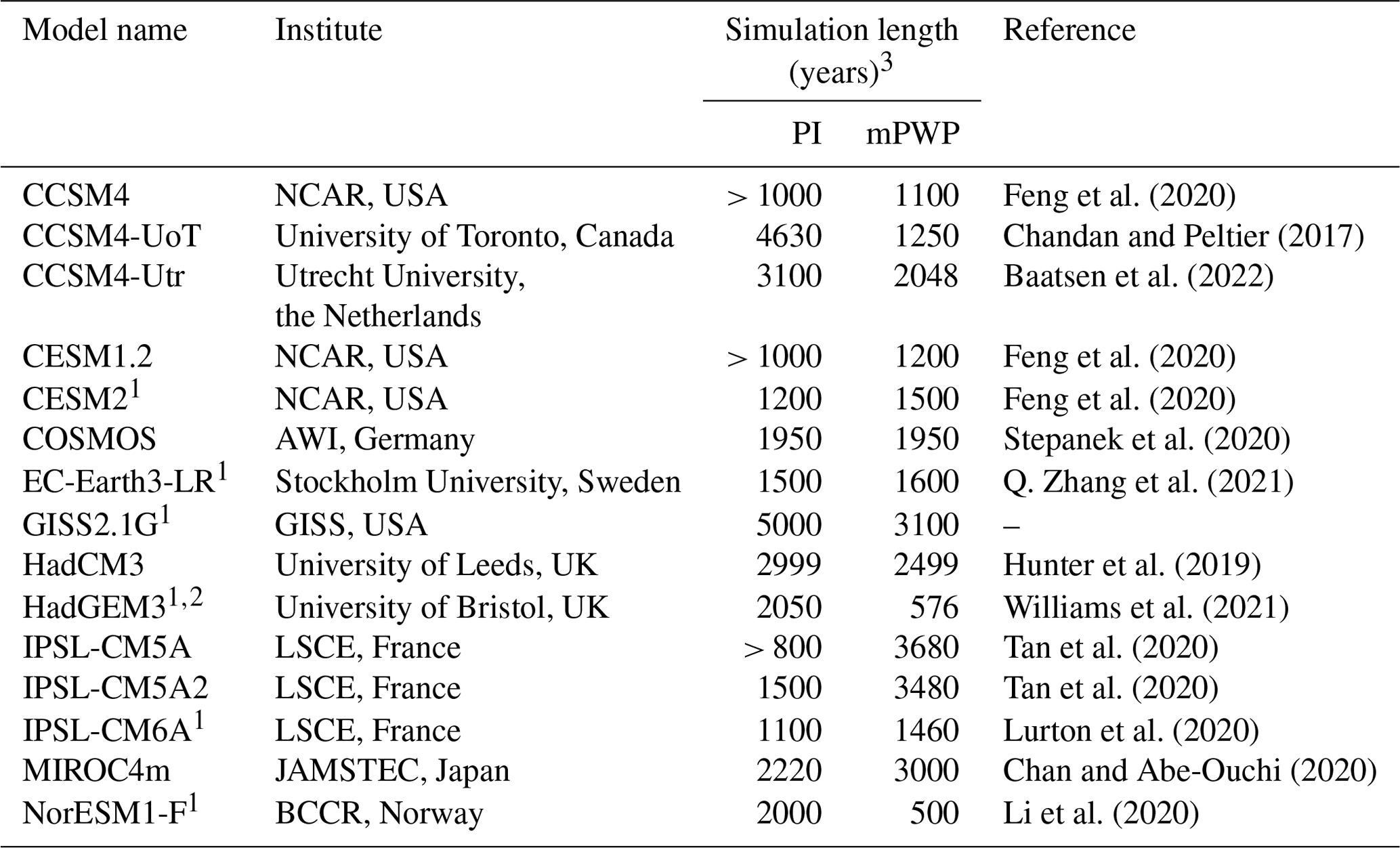
¹ CMIP6 model with pre-industrial 1850 CO₂ at 284.3 ppm. ² Pre-industrial land–sea mask in both simulations. ³ As presented in Z. Zhang et al. (2021).

2.2 Proxy data

To compare mid-Pliocene model results with reconstructed data, we use SST proxy data from a 30 kyr interval centered on the KM5c time slice by Foley and Dowsett (2019) and McClymont et al. (2020a). The PRISM4 dataset (Foley and Dowsett, 2019) is a collection of U${}_{\mathrm{37}}^{\text{K'}}$ proxies (calibrated using the Müller et al., 1998, method). The dataset by McClymont et al. (2020a) includes both U${}_{\mathrm{37}}^{\text{K'}}$ proxies (calibrated using the BAYSPLINE method) and foraminifera Mg/Ca proxy SST reconstructions. In this study, SST reconstructions from six different sites between 30 and 70^∘ N in the North Atlantic have been used. For comparison to model anomalies, the NOAA ERSST5 dataset (Huang et al., 2017) for the years 1870–1899 is used as the observational pre-industrial SST dataset.

2.3 Data analysis

All models except IPSL-CM5A and IPSL-CM5A2 have provided 100 years of annual model data for both E²⁸⁰ and Eoi⁴⁰⁰. IPSL-CM5A and IPSL-CM5A2 have provided 50-year averages only, so they are excluded from analysis that requires annual data.

Percentage differences between the mid-Pliocene and pre-industrial are computed relative to the pre-industrial. An anomaly is defined as the difference between the mid-Pliocene and pre-industrial (mPWP–PI, Eoi⁴⁰⁰–E²⁸⁰), unless stated otherwise. Standard deviations of individual model means are calculated using annual data. Standard deviations of MMM anomalies are calculated using the individual model Eoi⁴⁰⁰–E²⁸⁰ anomalies.

Data provided by individual modeling groups include the ocean potential temperature, ocean meridional velocity, ocean salinity, the Atlantic meridional streamfunction, the total Atlantic OHT, and the atmospheric zonal and meridional wind at 1000 hPa. In addition, the atmospheric surface freshwater flux (precipitation minus evaporation, PmE) fields for all models provided by Han et al. (2021) have been used. SST, sea surface salinity (SSS), PmE and atmospheric wind fields have been interpolated to a ${\mathrm{1}}^{\circ }\times {\mathrm{1}}^{\circ }$ regular grid using bilinear interpolation. All calculations for Atlantic Ocean heat transport and freshwater transport have been performed on model native grids, except for COSMOS, where it is done on the regular interpolated grid. These computations have been done using Atlantic region masks provided by the individual modeling groups. The mean AMOC strength is calculated from the 100-year mean Atlantic meridional overturning streamfunction and the yearly AMOC strength from the annual-mean Atlantic meridional overturning streamfunction. The AMOC strength is defined as the maximum value of the Atlantic meridional overturning streamfunction north of the Equator and below 500 m depth. Potential density is calculated from potential temperature and salinity using the TEOS-10 equation of state (Roquet et al., 2015).

2.3.1 Ocean heat transport

The 100-year mean OHT is defined at every latitude y as

$$\begin{array}{}\text{(1)}& \mathrm{OHT}={\mathit{\rho }}_{\mathrm{0}}{c}_p\int \underset{x_E}{\overset{x_W}{\int }}\stackrel{\mathrm{‾}}{vT}\mathrm{d}x\mathrm{d}z.\end{array}$$

Here, v is the meridional ocean velocity and T the ocean potential temperature of each grid cell of dx in longitude and dz in depth; the bar denotes a 100-year mean. The y dependency of the OHT is omitted in the notation. For the Atlantic OHT, integration is performed zonally between the eastern and western boundaries of the Atlantic Ocean, respectively x_E and x_W. The constants ρ₀ and c_p are the average density and specific heat of seawater, respectively. These are set at ${\mathit{\rho }}_{\mathrm{0}}=\mathrm{1.026}\times {\mathrm{10}}^{-\mathrm{3}}$ kg cm⁻³ and c_p=3996 J K kg⁻¹. In this study, the total OHT is calculated from the 100-year mean 3D meridional heat transport ($\stackrel{\mathrm{‾}}{vT}$) field. This total OHT can be partitioned into a mean flow OHT^M and a transient component OHT^T (Viebahn et al., 2016):

$$\begin{array}{}\text{(2)}& \mathrm{OHT}={\mathrm{OHT}}^{\mathrm{M}}+{\mathrm{OHT}}^{\mathrm{T}},\end{array}$$

where the time mean component OHT^M and transient component OHT^T are

$$\begin{array}{}\text{(3)}& {\displaystyle }{\mathrm{OHT}}^{\mathrm{M}}={\mathit{\rho }}_{\mathrm{0}}{c}_p\int \underset{x_E}{\overset{x_W}{\int }}\stackrel{\mathrm{‾}}{v}\stackrel{\mathrm{‾}}{T}\mathrm{d}x\mathrm{d}z\text{(4)}& {\displaystyle }{\mathrm{OHT}}^{\mathrm{T}}={\mathit{\rho }}_{\mathrm{0}}{c}_p\int \underset{x_E}{\overset{x_W}{\int }}\stackrel{\mathrm{‾}}{v^{\prime }{T}^{\prime }}\mathrm{d}x\mathrm{d}z.\end{array}$$

Here, $v=\stackrel{\mathrm{‾}}{v}+v^{\prime }$ and $T=\stackrel{\mathrm{‾}}{T}+T^{\prime }$, where $\stackrel{\mathrm{‾}}{v}$ and $\stackrel{\mathrm{‾}}{T}$ are the 100-year mean and v' and T' the transient components of the respective v and T fields. The 100-year mean $\stackrel{\mathrm{‾}}{vT}$, $\stackrel{\mathrm{‾}}{v}$ and $\stackrel{\mathrm{‾}}{T}$ are available from the model output; this allows us to deduce $\stackrel{\mathrm{‾}}{v^{\prime }{T}^{\prime }}$.

Next, we are able to separate OHT^M from (3) into two separate components associated with either the zonal-mean flow or the azonal flow. This will approximately separate OHT^M in heat transport that can be attributed to the overturning circulation (i.e., the zonal-mean flow) and heat transport that results from wind-driven gyre circulation (i.e., the azonal flow).

$$\begin{array}{}\text{(5)}& {\mathrm{OHT}}^{\mathrm{M}}={\mathrm{OHT}}_{\mathrm{ov}}+{\mathrm{OHT}}_{\mathrm{az}}\end{array}$$

Following Dijkstra (2007) and Viebahn et al. (2016),

$$\begin{array}{}\text{(6)}& {\displaystyle }{\mathrm{OHT}}_{\mathrm{ov}}={\mathit{\rho }}_{\mathrm{0}}{c}_p\int \underset{x_E}{\overset{x_W}{\int }}\langle \stackrel{\mathrm{‾}}{v}\rangle \langle \stackrel{\mathrm{‾}}{T}\rangle \mathrm{d}x\mathrm{d}z\text{(7)}& {\displaystyle }{\mathrm{OHT}}_{\mathrm{az}}={\mathit{\rho }}_{\mathrm{0}}{c}_p\int \underset{x_E}{\overset{x_W}{\int }}\langle {\stackrel{\mathrm{‾}}{v}}^{*}{\stackrel{\mathrm{‾}}{T}}^{*}\rangle \mathrm{d}x\mathrm{d}z.\end{array}$$

Here, $\langle \stackrel{\mathrm{‾}}{v}\rangle$ and $\langle \stackrel{\mathrm{‾}}{T}\rangle$ are the zonal average of $\stackrel{\mathrm{‾}}{v}$ and $\stackrel{\mathrm{‾}}{T}$, and ${\stackrel{\mathrm{‾}}{v}}^{*}$ and ${\stackrel{\mathrm{‾}}{T}}^{*}$ are the azonal components such that $\stackrel{\mathrm{‾}}{v}=\langle \stackrel{\mathrm{‾}}{v}\rangle +{\stackrel{\mathrm{‾}}{v}}^{*}$ and $\stackrel{\mathrm{‾}}{T}=\langle \stackrel{\mathrm{‾}}{T}\rangle +{\stackrel{\mathrm{‾}}{T}}^{*}$.

This method for separating the ocean heat transport into a component that can be attributed to the overturning circulation and a component attributed to the wind-driven gyre circulation is a conventional method introduced by Bryan (1982) and Hall and Bryden (1982). It has been used in many studies of both observational (e.g., Johns et al., 2011) and model data (e.g., Viebahn et al., 2016). That said, it is important to recognize that it does not perfectly separate the transport by the gyre circulation and overturning circulation. Attributing all zonal-mean circulation to the overturning circulation and all azonal flow to the gyre circulation is a simplification that inevitably introduces some error. An alternative method that may resolve problems with separating the overturning and gyre components near the western boundary and prevents the deep-ocean circulation from being attributed to the wind-driven gyre could be to separate out transport by the western boundary current of the gyre circulation and attribute heat transport in the deep ocean to the overturning circulation only. This requires a definition of the deep ocean, which could be achieved by identifying the level of no motion along the vertical axis and assigning all grid points below this level to the deep ocean. For the western boundary current, a longitude for the western boundary could be determined by integrating the meridional volume transport above the level of no motion from east to west until the total volume transport is zero. Heat transport east of this boundary and above the level of no motion can then be attributed to the gyre circulation and the rest of the heat transport to the overturning circulation. The reason why we have not implemented this method is that it introduces new problems and error due to challenges in accurately defining the boundary of the deep ocean and western boundary, in particular because the method has to be implemented for every model individually. Alternatively, a method that involves separating these components based on water mass ventilation, as done by Talley (2003), would also be interesting to implement as it is more accurate and would therefore allow for a more quantitative assessment of the error introduced by our method. However, the implementation of this method is complex, especially when it has to be carried out for each individual model, rendering it beyond the scope of this study.

It should be noted that the separation for the overturning and gyre components as shown above can only be done for the time mean component as instantaneous velocity fields are not available. Therefore, the total OHT will always contain a transient component OHT^T in addition to the mean overturning OHT_ov and gyre components OHT_az:

$$\begin{array}{}\text{(8)}& \mathrm{OHT}={\mathrm{OHT}}_{\mathrm{ov}}+{\mathrm{OHT}}_{\mathrm{az}}+{\mathrm{OHT}}^{\mathrm{T}}.\end{array}$$

The variability contained in the transient component OHT^T is primarily a result of the seasonal cycle and is therefore largely unaffected by the choice of averaging period (Viebahn et al., 2016). Only in areas of high eddy activity, primarily the Southern Ocean, is the transient component significant (Yang et al., 2015). Figure S1 in the Supplement shows a comparison between the total Atlantic OHT (OHT) and the time mean Atlantic OHT (OHT${}^{\mathrm{M}}={\mathrm{OHT}}_{\mathrm{ov}}+{\mathrm{OHT}}_{\mathrm{az}}$), where no significant discrepancy is found for most models. The exceptions are the COSMOS, HadCM3, GISS2.1G, MIROC4m and NorESM1-F. In COSMOS and HadCM3, this difference most likely occurs as a result of using surface heat fluxes at the sea surface to calculate the total OHT. As this approach requires assuming that there is no change in ocean heat storage and that all heat that vertically enters the ocean through the surface will be transported horizontally by the circulation (Yang et al., 2015), this may indicate that either or both of these conditions are not fulfilled in these models. For COSMOS, the absence of thermal equilibrium has been explicitly shown by Stepanek et al. (2020) and Lohmann et al. (2022). Therefore, we have used OHT^M that is calculated from the individual velocity and temperature fields as the total OHT for COSMOS and HadCM3. In addition, the calculated overturning OHT component from MIROC4m and COSMOS is quite noisy due to interpolation in the original velocity, temperature or region fields. This output is smoothed using a 5^∘ running mean.

For models with a curvilinear grid, the transport calculations on a native grid lead to a degree of error at higher latitudes due to the misalignment of the meridional velocity with the y direction of the grid cells. For this reason, the OHT components are only calculated up to 65^∘ N for all models.

2.3.2 Freshwater transport

The freshwater transport F is calculated for all model simulations using the 100-year mean meridional ocean velocity $\stackrel{\mathrm{‾}}{v}$ and salinity $\stackrel{\mathrm{‾}}{S}$ fields:

$$\begin{array}{}\text{(9)}& F=-{\displaystyle \frac{\mathrm{1}}{S_{\mathrm{0}}}}\int \underset{x_E}{\overset{x_W}{\int }}\stackrel{\mathrm{‾}}{v}(\stackrel{\mathrm{‾}}{S}-S_{\mathrm{0}})\mathrm{d}x\mathrm{d}z,\end{array}$$

where S₀ is the reference salinity, which is set to be the average Atlantic Ocean salinity for every individual simulation. The integration is performed over the ocean depth and Atlantic basin width as for the Atlantic OHT and calculated up to 65^∘ N due to curving of curvilinear grids. The freshwater transport is also calculated for two sections of the Atlantic Ocean at 62^∘ N west and east of Greenland, respectively referred to as the Labrador Sea and Greenland–Scotland Ridge (GSR) freshwater transports. Freshwater transport through the Bering Strait in the pre-industrial simulations is also computed.

In order to analyze the separate effect of the overturning and wind-driven gyre circulation on the Atlantic freshwater transport, the same separation of components is done as for the OHT, following Dijkstra (2007):

$$\begin{array}{}\text{(10)}& {\displaystyle }{F}_{\mathrm{ov}}=-{\displaystyle \frac{\mathrm{1}}{S_{\mathrm{0}}}}\int \underset{x_E}{\overset{x_W}{\int }}\langle \stackrel{\mathrm{‾}}{v}\rangle (\langle \stackrel{\mathrm{‾}}{S}\rangle -S_{\mathrm{0}})\mathrm{d}x\mathrm{d}z\text{(11)}& {\displaystyle }{F}_{\mathrm{az}}=-{\displaystyle \frac{\mathrm{1}}{S_{\mathrm{0}}}}\int \underset{x_E}{\overset{x_W}{\int }}\langle {\stackrel{\mathrm{‾}}{v}}^{*}{\stackrel{\mathrm{‾}}{S}}^{*}\rangle \mathrm{d}x\mathrm{d}z.\end{array}$$

This means that a similar degree of error is introduced when separating the freshwater transport into the overturning and a gyre component, as discussed above for the separation of the OHT components. In addition, total freshwater transport does not include the transient term in our study due to the use of 100-year mean velocity and salinity fields. This transient term is caused by seasonal variations in gyre circulation, similar to the transient OHT component, and surface salinity as well as baroclinic mesoscale eddies at the boundary of the subtropical and subpolar gyres (Treguier et al., 2012). We neglect the transient term as it was shown to be small at a model resolution of approximately 1^∘ (Jüling et al., 2021).

3 Results

Figure 1 gives an overview of the AMOC strength and its variability in the individual mid-Pliocene and pre-industrial simulations. We find that all models except CESM1.2 and HadGEM3 simulate a stronger AMOC in the Pliocene. This is a slightly different result from Z. Zhang et al. (2021), where CESM1.2 did simulate a stronger AMOC in the Pliocene. Discrepancies between AMOC strength reported by Z. Zhang et al. (2021) and Fig. 1 can be attributed to a difference in the 100-year time interval of the model data.

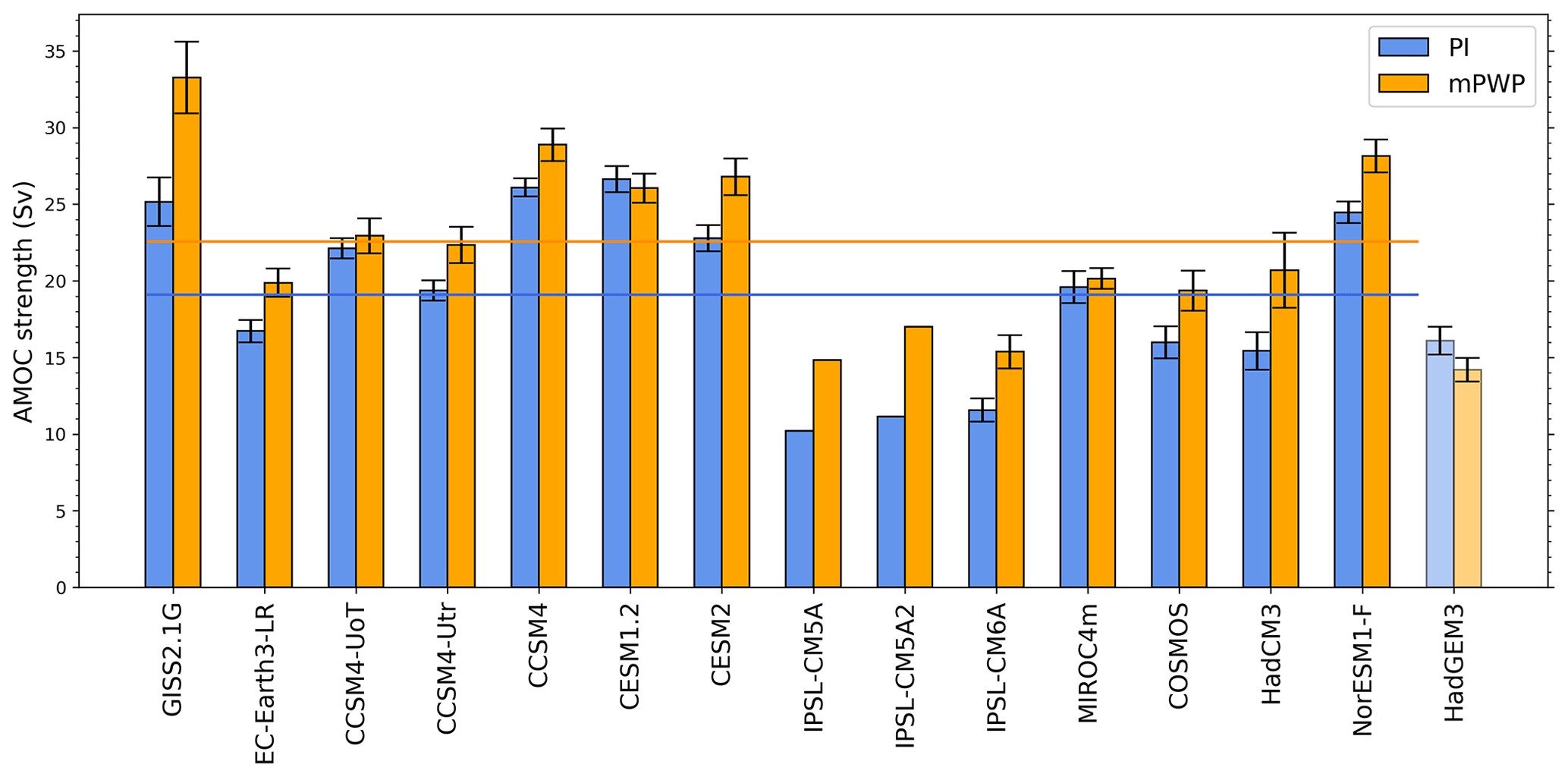
Figure 1 Individual model AMOC strength in the pre-industrial (blue) and mid-Pliocene (orange). Error bars indicate 1 standard deviation from the time-mean AMOC strength computed using 100 years of annual data. The horizontal lines indicate the multi-model mean AMOC strength.

The error bars in Fig. 1 show the standard deviation of the annual AMOC strength from the 100-year mean. The error bars for CESM1.2 show that the decrease in AMOC strength is not significant. This is also the case for the increase in AMOC strength in CCSM4-UoT and MIROC4m. For all other models included in this study, the intensified AMOC in the mid-Pliocene compared to the pre-industrial is significant. The only model simulating a significant decrease in AMOC strength is HadGEM3, presumably related to the pre-industrial land–sea mask configuration in the mid-Pliocene simulation as discussed in Z. Zhang et al. (2021). Also note that for the majority of the models, the variability in the AMOC strength increases in the mid-Pliocene, with the exception of MIROC4m and HadGEM3.

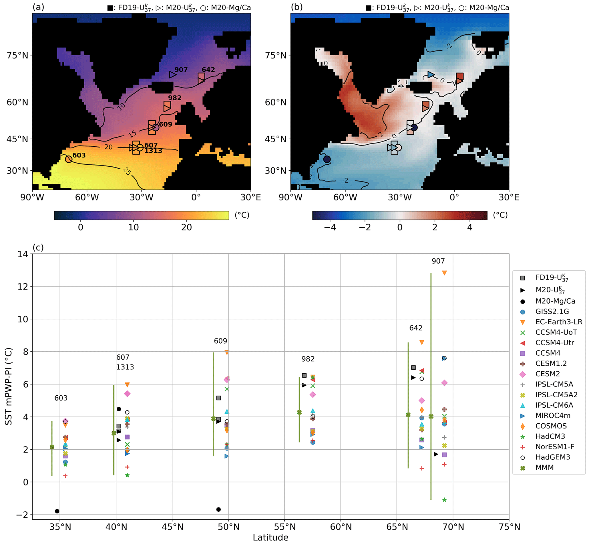
Figure 2 (a) Mid-Pliocene MMM and reconstructed North Atlantic SST. (b) MMM and reconstructed North Atlantic SST anomaly (mPWP–PI) with respect to the average MMM North Atlantic SST anomaly (30^∘ N–70^∘ N). (c) Individual model SSTs and reconstructed SSTs at six proxy locations in the North Atlantic. The vertical line shows the model spread, and the MMM (excluding HadGEM3) is indicated by a cross. FD19-U${}_{\mathrm{37}}^{\text{K'}}$ refers to the Foley and Dowsett (2019) data, M20-U${}_{\mathrm{37}}^{\text{K'}}$ and M20-Mg/Ca to the McClymont et al. (2020a) data. SST proxy anomalies are computed with pre-industrial ERSST5 data (Huang et al., 2017). The code to read and plot the proxy SST data has been adapted from Oldeman (2021).

3.1 North Atlantic SSTs linked to AMOC

3.1.1 Comparison of models with proxy data

Figure 2 compares the MMM and individual models' SSTs to U${}_{\mathrm{37}}^{\text{K'}}$ SST proxy data from Foley and Dowsett (2019) and U${}_{\mathrm{37}}^{\text{K'}}$ and Mg/Ca proxy data from McClymont et al. (2020a) at six different North Atlantic sites. These sites are chosen based on their location between 30–70^∘ N, excluding sites in proximity to the Mediterranean Sea. Figure 2a shows the SSTs in the mid-Pliocene and Fig. 2b the SST mPWP–PI anomalies with respect to the MMM 30–70^∘ N average North Atlantic mPWP–PI SST anomaly. Red-colored regions in Fig. 2b indicate above-average warming and blue-colored regions below-average warming with respect to the average 30–70^∘ N North Atlantic warming. This allows for a closer inspection of regional differences in extratropical North Atlantic warming. The modeled SST values at the different proxy sites can be found in Table S1 in the Supplement. Figure 2b indicates that the strongest amplified North Atlantic warming in the MMM mid-Pliocene SSTs occurs north of 45^∘ N and west of 30^∘ W, an area where there are currently no proxy data available for the KM5c time slice. Most proxy data originate from locations that are in the white area in Fig. 2b, meaning that the warming simulated there is approximately equal to the extratropical North Atlantic mean warming.

The mPWP–PI anomalies of the reconstructed SSTs and MMM SSTs are plotted in Fig. 2c, along with the individual model SST anomalies. We find that the discrepancy between reconstructed and MMM SST anomalies is smallest for sites $\mathrm{607}/\mathrm{1313}$ and 609, with the exception of the relatively cold Mg/Ca reconstruction at site 609. The sites where reconstructions indicate the strongest mid-Pliocene warming are sites 982 and 642. These sites are also the only two sites that fall within the area where MMM warming is higher than the North Atlantic 30–70^∘ N average, as seen in Fig. 2b, although they are both at the edge of this area. The sites north of 60^∘ N show a greater discrepancy between reconstructions and the MMM, as well as a relatively large model spread. The reconstructed SST at site 603 also does not agree with the MMM and falls outside the range of model SSTs, which may be related to its location in the highly variable Gulf Stream region. This region including the Gulf Stream separation is generally not well resolved in low-resolution general circulation models (Bryan et al., 2007; Saba et al., 2016; Schoonover et al., 2017). It may also be due to other factors such as calibration and seasonality affecting the Mg/Ca SST reconstructions (McClymont et al., 2020a) since we see that the Mg/Ca proxy SST values are much lower than the PlioMIP2 model range at site 609 as well.

3.1.2 Effect of the stronger mid-Pliocene AMOC

Even though we observe above-average warming of SSTs in the northwestern North Atlantic (Fig. 2b), it has been shown that average North Atlantic temperatures do not respond consistently to a stronger mid-Pliocene AMOC (Z. Zhang et al., 2021). To further examine the effect of a stronger mid-Pliocene AMOC on North Atlantic SSTs, we show correlation maps between annual-mean AMOC strength and SSTs at every grid point for both the pre-industrial and mid-Pliocene in Fig. 3. Grid points that are colored red show positive correlation between the SST and the AMOC strength, with positive correlations greater than 0.4 indicated by a white contour line.

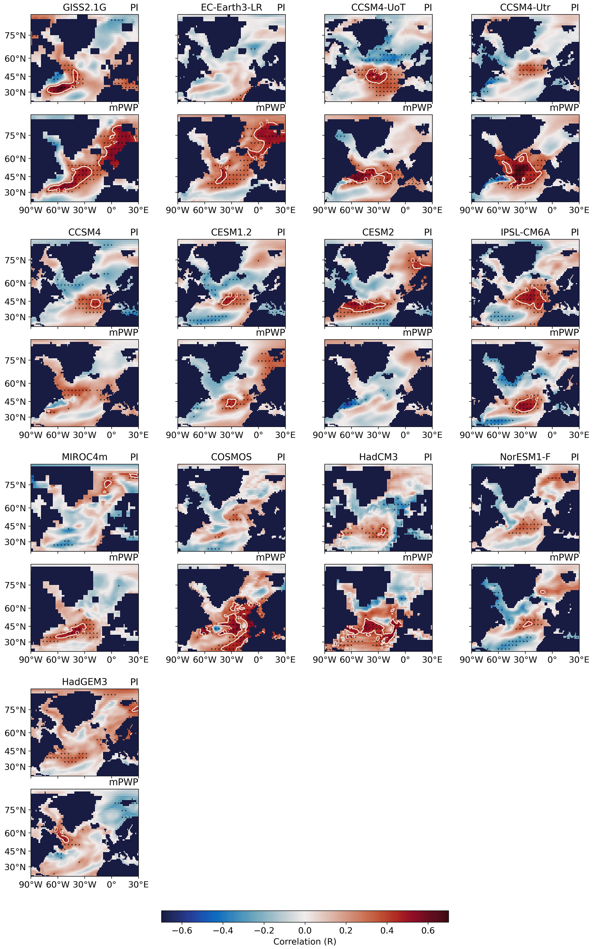
Figure 3 Correlation between the annual AMOC strength and annual SSTs for individual models. The top panel for each model shows the results for the pre-industrial, and the bottom panel shows the results for the mid-Pliocene. Both the AMOC strength and SSTs have been linearly detrended before correlating. Stippling indicates significance at the 95 % confidence level. White contours show a positive correlation of R=0.4.

The majority of the PlioMIP2 models show that the effect of the AMOC on North Atlantic SSTs is different in pattern in the mid-Pliocene from the pre-industrial, where for most models there is a relatively larger area of significant positive correlation in the mid-Pliocene (see Table S2). Furthermore, the positive correlation with SSTs is higher in the mid-Pliocene, with the exception of CCSM4, CESM1.2, CESM2, NorESM1-F, IPSL-CM6A and HadGEM3. CCSM4 and CESM2 do not have a stronger correlation between North Atlantic SSTs and the AMOC strength, but their maps do show a shift in the spatial pattern of correlation. The same is true for HadGEM3, which does not employ a mid-Pliocene land–sea mask and simulates a weaker mid-Pliocene AMOC. In CESM1.2, which has a weaker AMOC in the mid-Pliocene, as well as NorESM1-F and IPSL-CM6A, the correlation remains similar in strength and pattern. The results suggest that for the majority of the models, the stronger mid-Pliocene AMOC exerts a stronger influence on North Atlantic SSTs than in the pre-industrial. This would imply that a stronger mid-Pliocene AMOC also corresponds to higher North Atlantic temperatures. In the MMM correlation maps (Fig. S2) we see a consistent area of positive correlation in both the PI and mPWP that increases in extent and magnitude in the mPWP. It supports our individual model results in Fig. 3 but at the same time underscores the need to stress that the relation and the specific area where a stronger mid-Pliocene AMOC may be related to higher North Atlantic temperatures appear to be highly model-dependent.

3.2 Density-affected increase in AMOC strength

The AMOC is known to be affected by meridional gradients in density (Rahmstorf, 1996; Thorpe et al., 2001; Stouffer et al., 2006; Wang et al., 2010) where the relatively high density in the North Atlantic is linked to deep convection that constitutes the sinking branch of the AMOC in the high northern latitudes. It should be noted that the AMOC is driven by meridional pressure gradients that scale with ΔρH² (de Boer et al., 2010), with Δρ the meridional density gradient and H the depth of the maximum overturning streamfunction, and that a correlation with the density gradient is only expected if the depth of the overturning is not affected by processes that are not directly related to the strength of the AMOC. Given that the AMOC becomes stronger in almost all mid-Pliocene simulations relative to the pre-industrial, we now examine whether this is related to an increase in the meridional density gradient in Fig. 4. Figure 4a shows the zonal-mean MMM potential density of the top 1 km of the Atlantic Ocean, where it is clear that most of the Atlantic becomes less dense. This is also indicated by Fig. 4b, where the potential density from Fig. 4a is averaged over the top 1 km. However, for the higher northern latitudes, approximately 40–80^∘ N, we observe that the potential density decreases by about 0.1 kg m⁻³, which is substantially less than in the rest of the Atlantic, where the decrease is approximately 0.3 kg m⁻³. This results in an overall increase in the meridional density gradient, which is defined as the difference between the 50–70^∘ N average and 10–30^∘ S average for all models except GISS2.1G. In this specific model, significant deep-water formation takes place at latitudes higher than 70^∘ N in the mPWP (Fig. S3), and we have therefore extended the northern box to 50–80^∘ N for GISS2.1G. We have plotted the AMOC strength anomaly against the meridional density gradient anomaly for all individual models in Fig. 4c. This shows a clear relationship between the mPWP–PI change in density gradient and the AMOC strength, where a greater increase in density gradient correlates significantly (R=0.67, p=0.01) with a larger increase in AMOC strength.

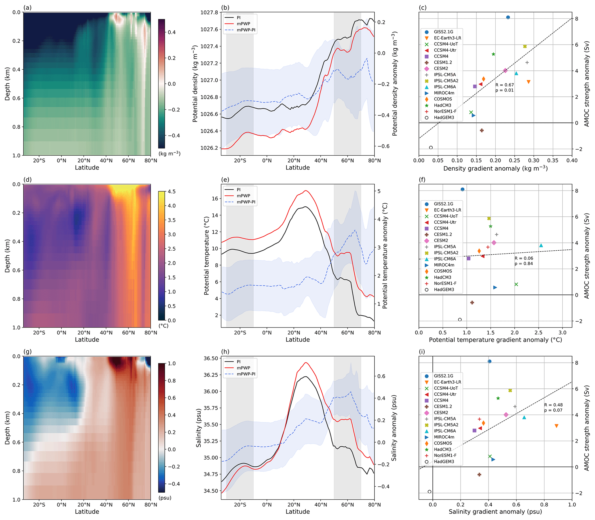
Figure 4 (a) MMM top 1 km Atlantic zonal-mean potential density mPWP–PI anomaly. (b) MMM top 1 km depth-averaged Atlantic zonal-mean potential density in the PI and mPWP (left y axis) and mPWP–PI anomaly (right y axis). Blue shading indicates 1 standard deviation from the MMM by individual models. (c) Individual model mPWP–PI AMOC strength anomaly plotted against the mPWP–PI anomaly in meridional gradient of the top 1 km Atlantic potential density. The meridional gradient is defined as the difference between the 50–70^∘ N average and 10–30^∘ S average (latitude bands are indicated by gray shading in (b). (d–f) Same as (a–c) for potential temperature. (g–i) Same as (a–c) for salinity.

Changes in density are brought about by changes in the potential temperature and salinity of the ocean. We show the potential temperature and salinity in the same manner as the potential density in Figs. 4d–f and g–i, respectively. As the North Atlantic becomes substantially warmer between 40–80^∘ N than the rest of the basin in the mid-Pliocene, temperature cannot explain the increase in meridional density gradient. This leaves salinity as the main driver of the increase in the meridional density gradient, which is supported by Fig. 4g–i. We see a zonal-mean freshening of the South Atlantic and tropics from the surface down to approximately 500 m. The rest of the basin shows an increase in salinity, with the exception of the surface at latitudes higher than 65^∘ N. A high salinity anomaly is found between 40–60^∘ N in the top 100 m, extending further downwards in some locations. The salinity anomaly results in an increase in the meridional salinity gradient in the mid-Pliocene, where a relationship between the increased salinity gradient and increased AMOC strength in the mid-Pliocene is shown in Fig. 4i. Overall, Fig. 4 shows that the meridional density gradient increase affecting the AMOC strength must be a result of increased salinity in the high North Atlantic. This is supported by further analysis of the northern and southern boxes in Fig. S4, which shows the correlation plots from Fig. 4 for the individual boxes. There we find that density anomalies in both boxes correlate well with the AMOC strength but that it is only in the northern box that salinity anomalies show a significant correlation with the AMOC.

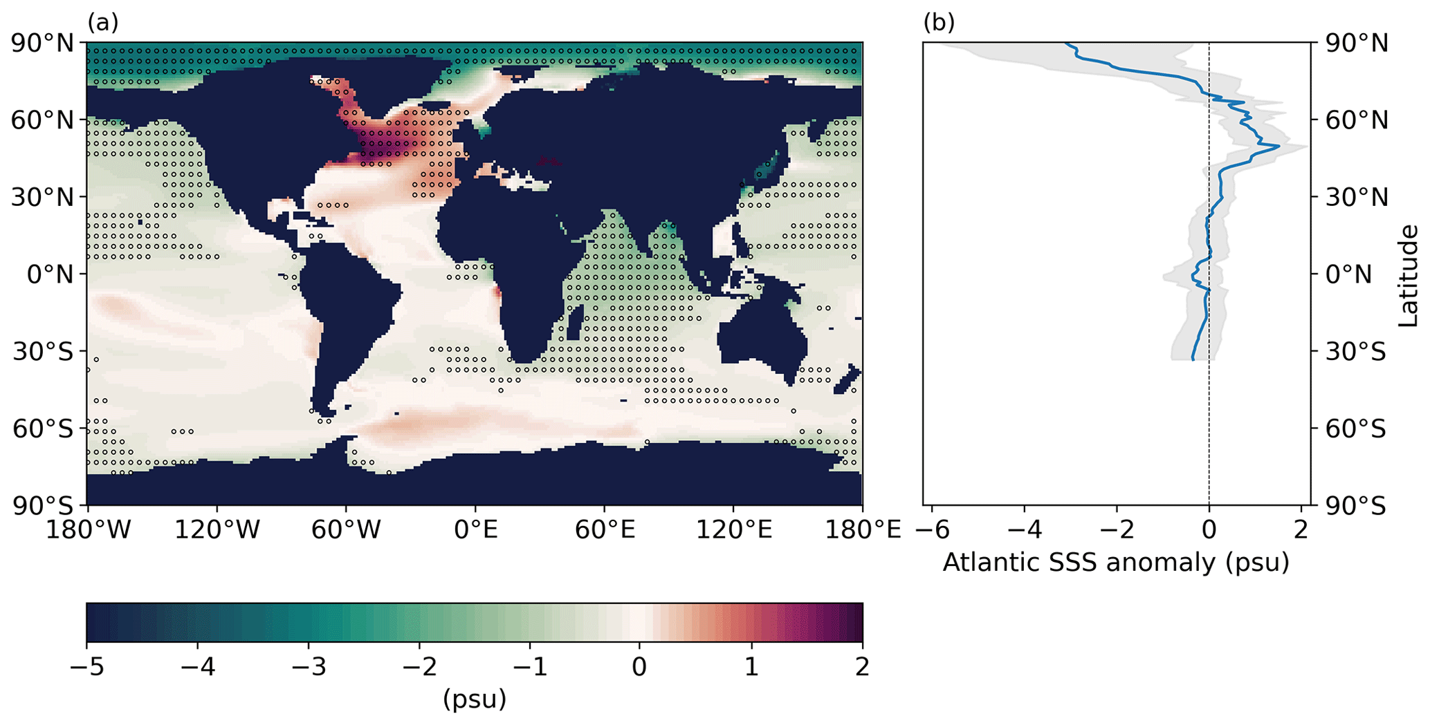
Figure 5 (a) Multi-model mean mPWP–PI difference in sea surface salinity (SSS). Stippling indicates that 12 or more models agree on the sign of the difference. (b) Atlantic zonal-mean SSS anomaly, excluding the Mediterranean Sea and North Sea. The shading indicates 1 standard deviation from the MMM by individual models.

3.2.1 Sea surface salinity

The consistent intensification of the mid-Pliocene AMOC across the PlioMIP2 ensemble compared to the PlioMIP1 ensemble is suggested to be linked to the closure of the Arctic gateways in PlioMIP2 (Haywood et al., 2020; Z. Zhang et al., 2021). Closing these Arctic gateways has been shown to cause an intensification of the AMOC through the decrease in freshwater transport from the Arctic into the North Atlantic via the Labrador Sea. This increases the salinity in the Labrador Sea and subpolar North Atlantic, thereby stimulating deep-water formation in these areas (Otto‐Bliesner et al., 2017). In the previous section we show that there is a substantial increase in the MMM salinity in the 40–60^∘ N latitude band in the North Atlantic. From the MMM sea surface salinity (SSS) in Fig. 5a, we can identify a robust increase of approximately 2 PSU in sea surface salinity in the Labrador Sea and in the North Atlantic between 40–60^∘ N. It is exclusively at these latitudes that we find the Atlantic zonal-mean sea surface salinity anomaly to be significantly positive (Fig. 5b) when considering the standard deviation of the individual models. All models forced with the PRISM4 reconstruction in the mid-Pliocene show this increase in sea surface salinity, as can be seen in Fig. S5. The fact that the HadGEM3 model, using a pre-industrial land–sea mask, does not show a sea surface salinity increase in the subpolar North Atlantic or Labrador Sea strengthens the argument that the stronger mid-Pliocene AMOC can be linked to the closure of the Arctic gateways in the PlioMIP2 simulations.

Even though the Bering Strait is closed in the mid-Pliocene experiments, blocking freshwater transport from the Pacific into the Arctic Ocean, a 3–4 PSU decrease in sea surface salinity in the Arctic Ocean can be seen in Fig. 5a. This decrease is present in all models except GISS2.1G, but the extent and magnitude of the decrease is highly model-dependent (Fig. S5). The decreased Arctic sea surface salinity may be explained by a higher surface freshwater flux into the Arctic Ocean in the mid-Pliocene as a result of atmospheric warming (Haywood et al., 2020; Han et al., 2021). This increase in surface freshwater flux over the Arctic Ocean that is consistent across the PlioMIP2 ensemble can be seen in Fig. 6a. The atmospheric freshwater flux is defined as the difference between the precipitation and evaporation (PmE), where a positive PmE means that precipitation exceeds evaporation at the surface. Other possible factors include an increase in runoff due to the reduced Greenland Ice Sheet and a decrease in sea ice extent in the mid-Pliocene (de Nooijer et al., 2020).

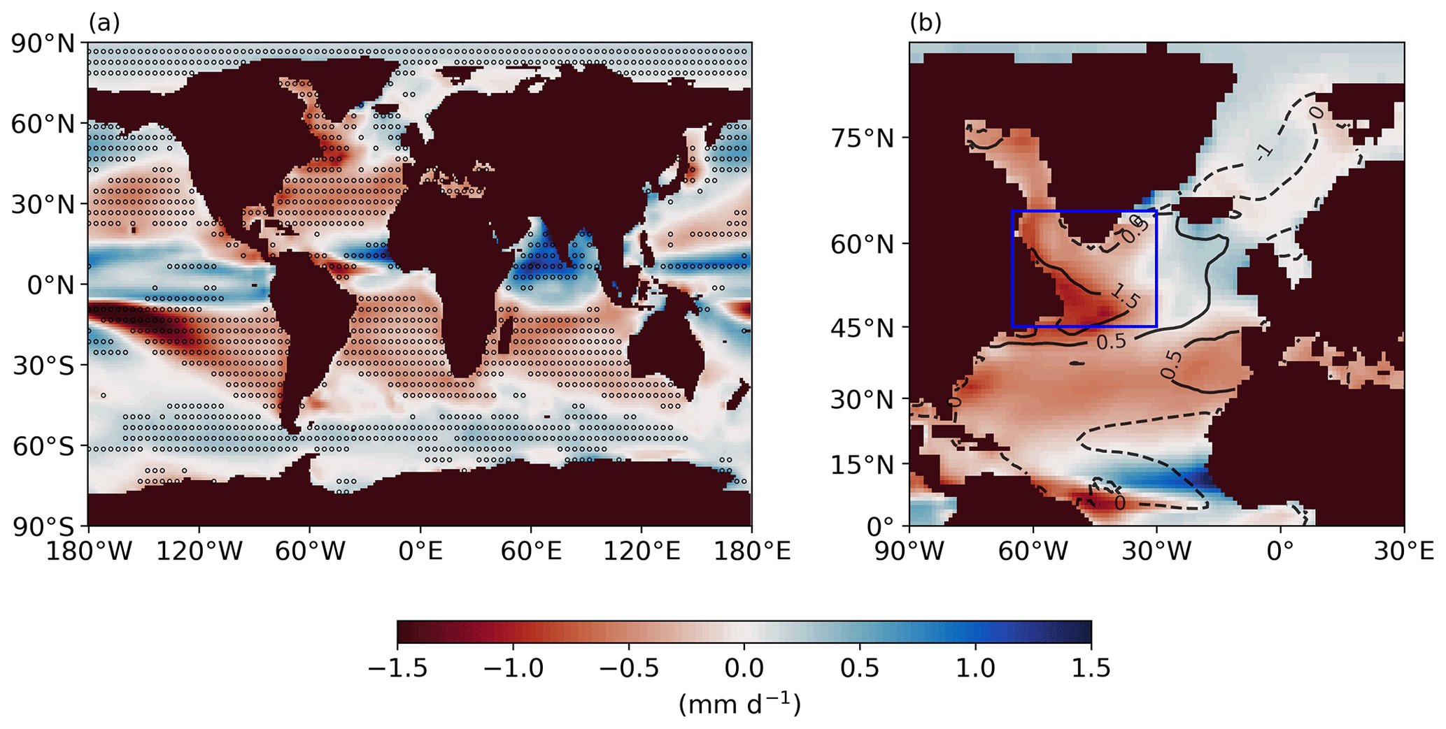
Figure 6 (a) Multi-model mean mPWP–PI difference in surface freshwater flux. Stippling indicates that 12 or more models agree on the sign of the difference. (b) Shading shows the MMM mPWP–PI difference in surface freshwater flux in the North Atlantic. Black contours show the MMM mPWP–PI sea surface salinity anomaly. The approximate extent of the negative PmE anomaly over the Labrador Sea and subpolar North Atlantic is indicated in (b) by the blue box (45–65^∘ N, 30–60^∘ W). A negative PmE anomaly means that evaporation is higher than precipitation.

Changes in the surface freshwater flux in the mid-Pliocene not only affect the Arctic Ocean salinity but also play a considerable role in the strongly increased North Atlantic sea surface salinity. Figure 6b allows us to consider the role that the atmospheric freshwater flux plays in the increased sea surface salinity in the Labrador Sea and part of the mid-Pliocene subpolar North Atlantic. Shading in Fig. 6b shows the MMM PmE anomaly, and the sea surface salinity anomaly is indicated by the black contours. We can see here that the surface freshwater flux is decreased over a considerable section of the subpolar North Atlantic despite an increase in MMM precipitation that has been shown in earlier work (Haywood et al., 2020). Off the coast of Newfoundland, the PmE shading follows sea surface salinity contours quite closely, which is an indication that the sea surface salinity is influenced by changes in surface freshwater flux there.

In the next subsection, we investigate how the mid-Pliocene boundary conditions affect freshwater transport between the Arctic, North Pacific and North Atlantic. Following from that, we consider the role that the surface freshwater flux and the freshwater transport play in the increase in the Atlantic Ocean sea surface salinity in the mid-Pliocene.

3.2.2 Freshwater transport

In the pre-industrial simulations, freshwater exchange between the Atlantic Ocean and the Pacific Ocean occurs both at 34^∘ S and through the Bering Strait. The Pacific water that is transported to the Arctic through the Bering Strait is relatively fresh. As the Arctic freshwater is then transported to the Atlantic Ocean via the Canadian Archipelago and Fram Strait into the Labrador and Norwegian seas, it dampens convection and deep-water formation in the high North Atlantic. As mentioned in earlier sections, it has been shown that closing the Bering Strait and Canadian Archipelago decreases the freshwater transport into and out from the Arctic Ocean (Hu et al., 2015; Otto‐Bliesner et al., 2017), promoting stronger deep-water formation in the North Atlantic. In this section, we take a closer look at both the freshwater transport through the whole Atlantic basin and the exchange of freshwater between the North Pacific and Arctic through the Bering Strait and between the Arctic and North Atlantic via the Fram Strait and Labrador Sea.

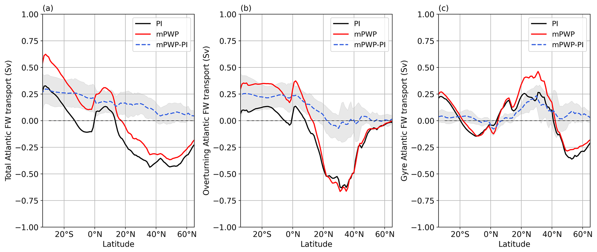
Figure 7 (a) MMM total Atlantic freshwater transport in the mid-Pliocene and pre-industrial and the difference. (b) MMM Atlantic freshwater transport by overturning. (c) MMM Atlantic freshwater transport by wind-driven gyres. The shading indicates 1 standard deviation of deviation from the MMM difference by individual models.

Figure 7a shows that the MMM southward total freshwater transport into the Atlantic Ocean at 65^∘ N decreases by 0.04 Sv (−19 %) in the mid-Pliocene. This presumably contributes significantly to the higher MMM sea surface salinity in the North Atlantic shown in Fig. 5. At 34^∘ S, the southern boundary of the Atlantic Ocean, the MMM northward transport of freshwater increases by 0.27 Sv (+96 %) in the mid-Pliocene. Using Fig. 7b and c, we can determine whether changes we observe in the total freshwater transport can be attributed to changes in the overturning or gyre circulation. Looking at the freshwater imported at the southern Atlantic boundary in Fig. 7b and c, it is clear that the higher mid-Pliocene import of freshwater at the southern boundary can be attributed almost entirely to the overturning circulation. However, in the North Atlantic the change in Atlantic freshwater transport by overturning is relatively small and inconsistent at latitudes higher than 20^∘ N. At latitudes above 20^∘ N, differences in the total Atlantic freshwater transport between the mid-Pliocene and pre-industrial can primarily be linked to the wind-driven gyre circulation, as can be seen in Fig. 7c. The freshwater transport by the (northern) subtropical gyre is almost doubled in the mid-Pliocene, while the transport by the subpolar gyre is decreased at latitudes higher than 50^∘ N.

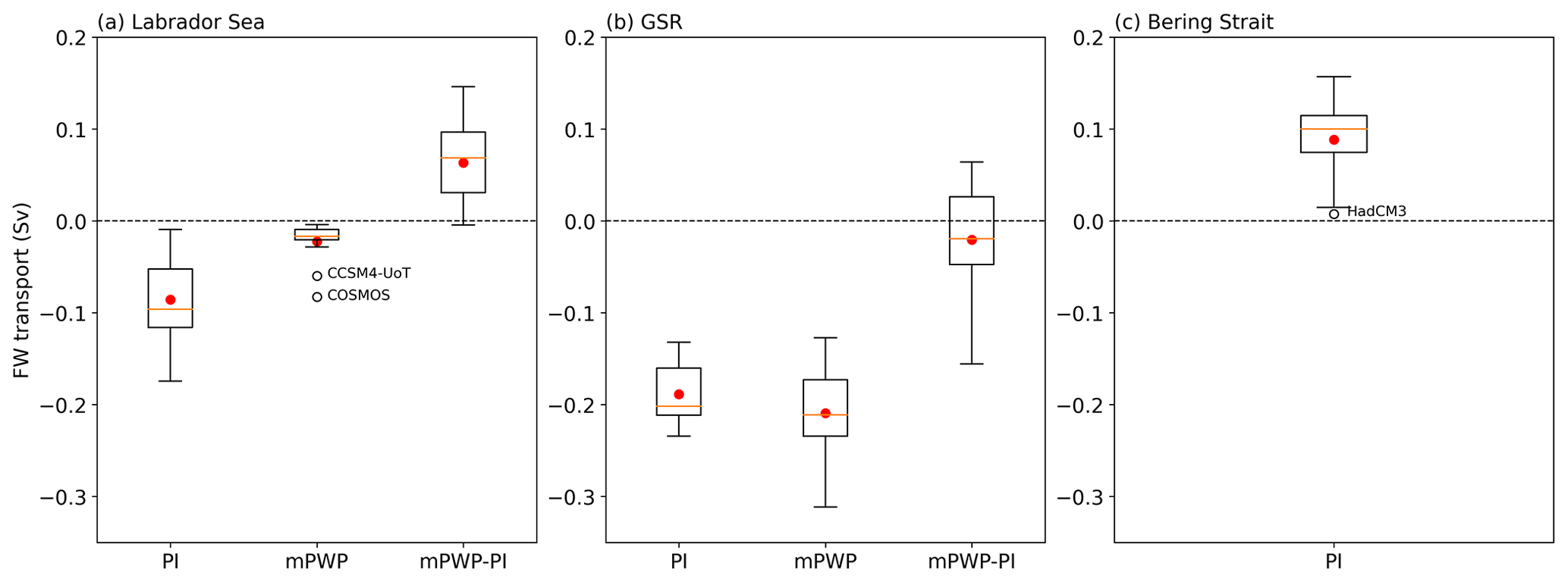
Figure 8 Boxplots of the mean freshwater transport (Sv) in the pre-industrial and mid-Pliocene and their difference at 62^∘ N (a) near the northern boundary of the Labrador Sea and (b) across the GSR. (c) Mean freshwater transport (Sv) through the Bering Strait in the pre-industrial. The box covers Q1 (25th percentile) to Q3 (75th percentile), with the median indicated by a horizontal orange line. The whiskers extend from Q1 to Q1–1.5 × IQR (interquartile range) and from Q3 to Q3+1.5 × IQR, where IQR $=Q\mathrm{3}-Q\mathrm{1}$. A model that falls outside the whiskers is separately shown as an unfilled circle. The MMM is indicated by a filled red circle.

To better understand how the mid-Pliocene boundary conditions impact the freshwater transport from the Arctic into the Atlantic Ocean, we differentiate between the total freshwater transport on the western and eastern side of Greenland at 62^∘ N in Fig. 8a and b. The freshwater transport on the western side of Greenland is entering the Labrador Sea, and the transport on the eastern side is going across the Greenland–Scotland Ridge (GSR). Note that in the mid-Pliocene, freshwater entering the Labrador Sea from the north cannot originate from the Arctic Ocean and can only result from runoff and the surface freshwater flux into Baffin Bay.

All model simulations show freshwater transport southwards into the Labrador Sea in both the pre-industrial and mid-Pliocene, regardless of an open or closed Canadian Archipelago (see Fig. S7 for individual model results). However, the MMM freshwater transport into the Labrador Sea (Fig. 8a) decreases dramatically with 0.063 Sv (−74 %) from the pre-industrial to the mid-Pliocene. We do not observe this decrease in HadGEM3. In Fig. 8b, we can see that the MMM freshwater transport increase of 0.021 Sv (+11 %) across the GSR in the mid-Pliocene is relatively small and compensates a third of the decrease in freshwater transport into the Labrador Sea. In addition, the box plots indicate that the decrease in freshwater transport into the Labrador Sea is a more consistent feature among the models than the increase in freshwater transport across the GSR. These results are in line with the decrease in the MMM total freshwater transport from the Arctic Ocean to the Atlantic Ocean in the mid-Pliocene (Fig. 7a). The decrease in total freshwater transport into the North Atlantic may partly be explained by the closure of the Bering Strait in the mid-Pliocene, causing a MMM freshwater transport decrease of 0.09 Sv into the Arctic (Fig. 8c). It has also previously been shown that closing the Bering Strait leads to less freshwater transported from the Arctic into the North Atlantic (Hu et al., 2015) due to effects on sea ice motion and freshwater exchange.

While our results show a robust decrease in freshwater transport from the Arctic into the North Atlantic, our freshwater transport calculations do not take into account the sea ice extent, which plays an important role in the Arctic freshwater balance (Aagaard and Carmack, 1989). However, all models show a greatly reduced sea ice cover in the Labrador Sea and Baffin Bay, and in most models the annual sea ice coverage does not extend southwards to 62^∘ N in the mid-Pliocene (Fig. S8). Therefore, qualitatively, our results should not be impacted if transport of sea ice were to be taken into account.

3.2.3 Role of surface freshwater flux and freshwater transport in increased North Atlantic salinity

In the previous subsections we show that the increase in North Atlantic sea surface salinity in the mid-Pliocene appears to be linked to changes in both the freshwater transport and the surface freshwater flux in the North Atlantic. We consider their respective roles in Fig. 9. We find a strong and significant correlation ($R=-\mathrm{0.92}$, p<0.05) between the mPWP–PI surface freshwater flux anomaly and the sea surface salinity anomaly in the Labrador Sea and eastern subpolar North Atlantic. There is also a moderately strong and significant correlation ($R=-\mathrm{0.53}$, p=0.04) between the mPWP–PI freshwater transport through the Bering Strait and the sea surface salinity anomaly, as well as a correlation of similar strength between the mPWP–PI freshwater transport at the northern boundary of the Labrador Sea and the sea surface salinity anomaly (R=0.48, p=0.07) that falls just outside the 95 % confidence level. The freshwater transport across the GSR does not correlate significantly with the North Atlantic sea surface salinity.

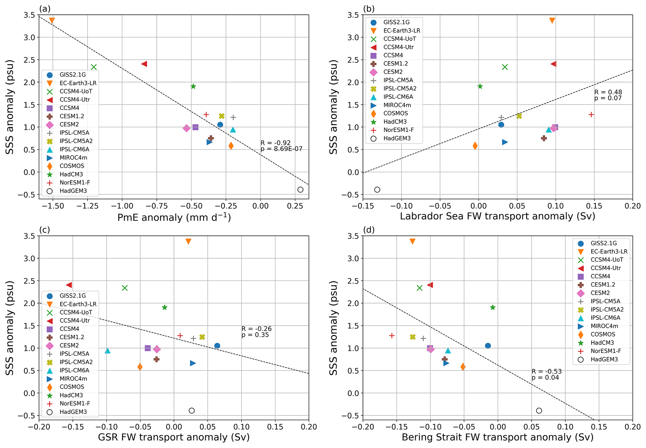
Figure 9 The mPWP–PI change in sea surface salinity plotted against (a) the mPWP–PI change in PmE freshwater flux, (b) the mPWP–PI change in northward freshwater transport at the northern boundary of the Labrador Sea (62^∘ N), (c) the mPWP–PI change in northward freshwater transport across the GSR (62^∘ N) and (d) the mPWP–PI change in northward freshwater transport across the Bering Strait. The sea surface salinity and PmE anomalies are averaged over the eastern subpolar North Atlantic and Labrador Sea (45–65^∘ N, 30–60^∘ W; the area indicated by the blue box in Fig. 6b).

The results from Fig. 9 indicate that there is a link between both the surface freshwater flux and the meridional freshwater transport with the increased North Atlantic salinity, but we cannot separate their respective strengths. While Otto‐Bliesner et al. (2017) identify decreased freshwater transport due to the closure of Arctic gateways as a mechanism for increasing the AMOC strength, our analysis shows that the decreased surface freshwater flux must also play a considerable role. However, the freshwater transport and surface freshwater flux are not independent of each other. Our results point to a complex interplay between different components of the North Atlantic freshwater balance in the mid-Pliocene simulations that combine to result in an increase in North Atlantic salinity and thereby density, ultimately affecting the AMOC strength. As with the sea surface salinity, we see that HadGEM3 does not show the same sign of change in the North Atlantic surface freshwater flux as the rest of the ensemble (Fig. S9). This further supports the notion that changes in the land–sea mask in the mid-Pliocene play an important role in the change in surface freshwater flux, potentially also linking it to the closure of the Arctic gateways.

3.3 Consequences of the stronger AMOC

3.3.1 Ocean heat transport

For all models with an intensified mid-Pliocene AMOC, we would expect the Atlantic OHT in the Northern Hemisphere to also be strengthened in the mid-Pliocene simulations. However, Fig. 10a shows that while the MMM total Atlantic OHT does increase at some latitudes, this increase is relatively small, with a maximum of 0.09 PW (+9 %) at 24^∘ N. Figure 10b and c show the relative contributions of the overturning and wind-driven gyre circulation to the MMM OHT. The MMM Atlantic OHT by overturning increases significantly more than the total Atlantic OHT in the NH with a maximum of 0.20 PW (+23 %) at 24^∘ N. Between 20–40^∘ N, this increase is robust across the ensemble when considering the standard deviation.

While the heat transported by the overturning circulation increases in the mid-Pliocene North Atlantic Ocean, the MMM gyre Atlantic OHT decreases (see Fig. 10c). This decrease is strongest in the region of the subtropical gyre, with a maximum decrease of −0.12 PW (−15 %) at 30^∘ N and a decrease of −0.10 PW (−12 %) at 24^∘ N. This suggests that the gyre circulation responds to mid-Pliocene conditions in such a way that it compensates for approximately half of the increase in Atlantic OHT by overturning in the subtropical North Atlantic. When we consider only the latitudes of the subtropical North Atlantic, 20–40^∘ N, we find that the 20–40^∘ N average MMM total Atlantic OHT at these latitudes increases by 0.07 PW (+9 %), and the overturning Atlantic OHT increases by more than twice this value: 0.16 PW (+21 %).

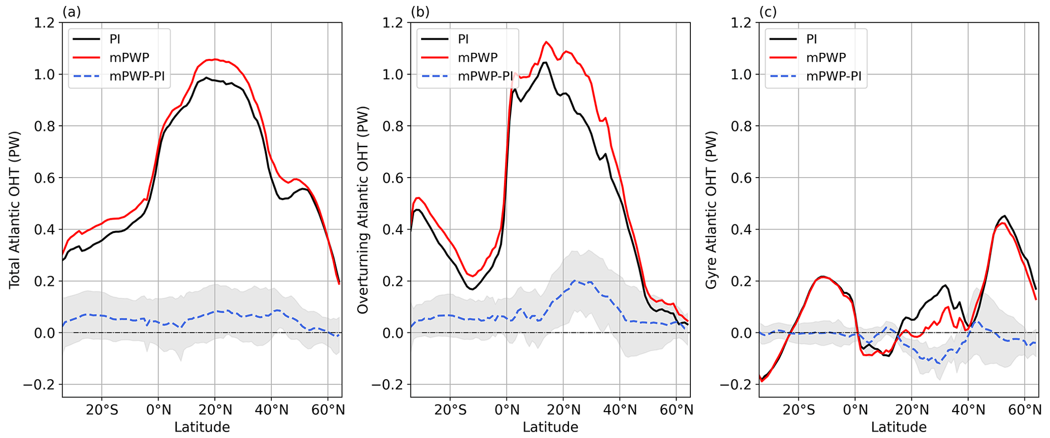
Figure 10 (a) MMM total Atlantic Ocean heat transport in the mid-Pliocene and pre-industrial and the difference. (b) MMM Atlantic Ocean heat transport by overturning. (c) MMM Atlantic Ocean heat transport by wind-driven gyres. The shading indicates 1 standard deviation by individual models from the MMM.

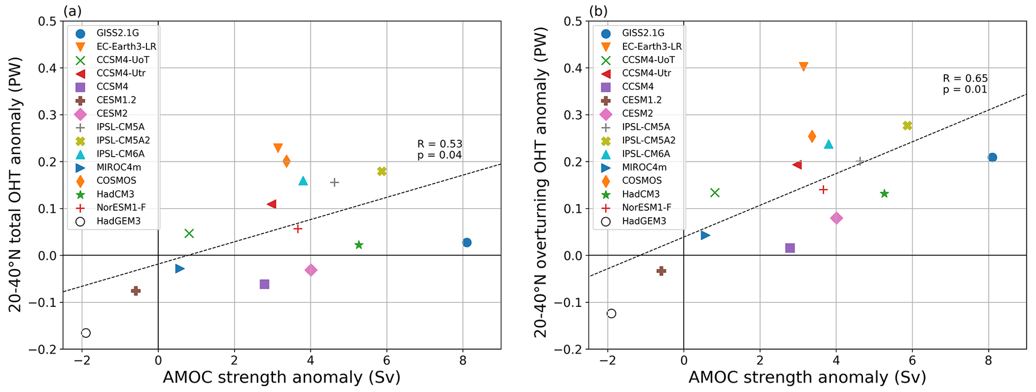
Figure 11 (a) The mPWP–PI change in average total Atlantic OHT between 20–40^∘ N and change in AMOC strength. (b) The mPWP–PI change in overturning Atlantic OHT between 20–40^∘ N and change in AMOC strength. The dotted line indicates a linear fit by least squares with the correlation coefficient R and p value of fit shown.

Table 2 Results of least squares linear fit between the mPWP–PI OHT anomaly and the AMOC strength anomaly. The latitude range indicates the latitudes over which the OHT has been averaged.

Figure 11 shows the mPWP–PI change in AMOC strength and total and overturning Atlantic OHT for all models. The OHT is averaged over 20–40^∘ N for three reasons: the influence of the overturning circulation on the Atlantic OHT is largest between 20–40^∘ N, it is the region where the subtropical gyre also influences the OHT, and most mid-Pliocene simulations show amplified SST warming in the Atlantic Ocean above 40^∘ N. When we compare changes in AMOC strength to those in the total OHT, not all models show that a stronger AMOC is accompanied by a higher total Atlantic OHT. However, when considering the OHT by overturning, all models with an intensified mid-Pliocene AMOC also have enhanced Atlantic OHT by overturning. A linear least-squares regression performed on the AMOC and overturning OHT reveals a slope that is 42 % higher than the slope of the regression between the AMOC and total OHT, as well as a better fit indicated by a higher R² and substantially lower p value. This result indicates that OHT components should be considered separately when looking at the response of the Atlantic OHT to a stronger mid-Pliocene AMOC.

In Table 2, the results of least-squares linear fits between the total OHT and the AMOC strength and the overturning OHT and the AMOC strength are shown for different latitude ranges over which the OHT is averaged. When considering the majority of the Atlantic Ocean basin (30^∘ S–60^∘ N), the regression shows an increased slope and R² value when performing it on the overturning OHT component rather than on the total OHT. We have performed the regressions also when excluding EC-Earth3-LR, which is an outlier in Fig. 10a and b due to its exceptionally large OHT increase. When EC-Earth3-LR is excluded, the R² increases significantly for all cases, especially for the regression with the overturning OHT, without substantial changes in the slope. In addition, the y intercept is closer to zero, and the p value decreases dramatically for the overturning OHT. Overall, these results suggest that the overturning OHT is a better indicator of the direct response of the OHT to a stronger AMOC in the mid-Pliocene. The PlioMIP2 ensemble shows a rather consistent response in the Atlantic OHT associated with overturning, where a stronger AMOC leads to enhanced Atlantic OHT by overturning.

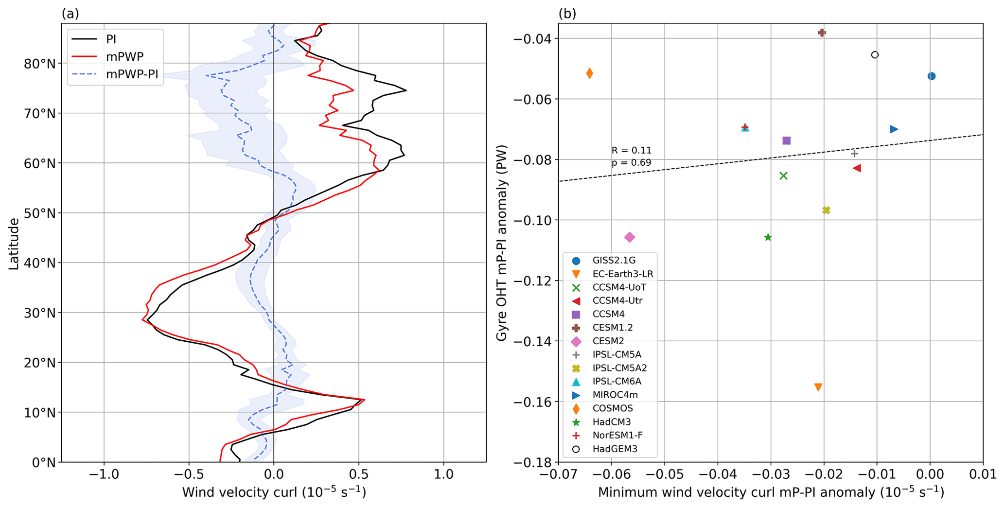
Figure 12 (a) MMM Atlantic zonal-mean 1000 hPa wind velocity curl $\left(\frac{\text{d}v}{\text{d}x}-\frac{\text{d}u}{\text{d}y}\right)$ in the pre-industrial and mid-Pliocene and their difference. Shading indicates 1 standard deviation from the MMM difference by individual models. (b) The minimum zonal-mean 1000 hPa wind velocity curl between 20–40^∘ N plotted against the 20–40^∘ N average OHT gyre component anomaly for individual models.

3.3.2 Transports by the subtropical gyre

Figure 10c showed that the MMM Atlantic OHT by the wind-driven gyre circulation shows a substantial decrease in the (northern) subtropical gyre region. At the same time, the MMM Atlantic freshwater transport of the northern subtropical gyre is almost doubled in the mid-Pliocene (Fig. 7c), meaning that less salt is being transported northwards by the subtropical gyre circulation. One possibility is that the subtropical gyre circulation itself responds to mid-Pliocene conditions through its coupling to the atmosphere. As wind stress fields are not available for the entire PlioMIP2 ensemble, we investigate changes in surface winds that drive the gyre circulation in Fig. 12. Figure 12a shows the zonal-mean curl of the MMM wind velocity at 1000 hPa in the North Atlantic. A positive wind velocity curl is associated with counterclockwise motion, the subpolar gyre, and a negative wind velocity curl is associated with clockwise motion, the subtropical gyre. The wind velocity curl in the subpolar region shows a substantial decrease, indicating weakening of the subpolar gyre circulation. In the subtropical gyre region, there is a shift in the wind velocity curl minimum towards higher latitudes, but we do not see a significant change in magnitude of the MMM zonal-mean wind velocity curl. This result indicates that there are no substantial changes in the mid-Pliocene wind circulation driving the subtropical gyre, and thus not in the subtropical gyre circulation itself. The lack of change in the subtropical gyre circulation is confirmed by the upper 500 m ocean meridional velocity, averaged over the 20–40^∘ N latitude band, which is similar in the mid-Pliocene and pre-industrial outside of the highly variable Gulf Stream region (Fig. S10). Figure 12b also does not suggest a connection between changes in the surface winds and the OHT by the subtropical gyre. No consistent relationship can be found between the minimum wind velocity curl in the subtropical gyre region and Atlantic OHT by the subtropical gyre when performing a least-squares linear regression (R=0.11, p=0.69). Therefore, we do not see any changes in the subtropical gyre circulation that could explain the substantial decrease in OHT by the gyre between 20–40^∘ N.

Without substantial changes to the wind-driven gyre circulation itself, changes in OHT and freshwater transport by the subtropical gyre may be linked to zonal asymmetry in the mPWP–PI anomalies in temperature and salinity. A zonal asymmetry in temperature or salinity could lead to more transport on the eastern or western part of the Atlantic basin, influencing the total gyre transport. Figure 13a and b show the difference between mid-Pliocene and pre-industrial SST and SSS, respectively, for the subtropical gyre region. A zonal asymmetry can be seen in both fields, with the eastern Atlantic becoming relatively warmer and saltier than the western Atlantic in the mid-Pliocene. When taking the meridional average over 20–40^∘ N for the SST and SSS, we find a zonal gradient in SST and SSS anomalies in Fig. 13c and d. For each model, the change in zonal SST gradient averaged between −20 and −70^∘ E (shaded gray in Fig. 13c) is plotted against the Atlantic gyre OHT anomaly in Fig. 13e. This reveals a significant negative correlation ($R=-\mathrm{0.79}$, p<0.05), meaning that a larger zonal gradient in SST anomalies corresponds to a larger decrease in OHT by the gyre. The same plot is shown for the average zonal gradient in the SSS anomalies and the Atlantic gyre freshwater transport in Fig. 13f. While the relationship is less robust than that between the SST gradient and OHT, a significant positive correlation (R=0.66, p<0.05) is found where a larger gradient in SSS anomalies is related to more northward freshwater transport by the subtropical gyre.

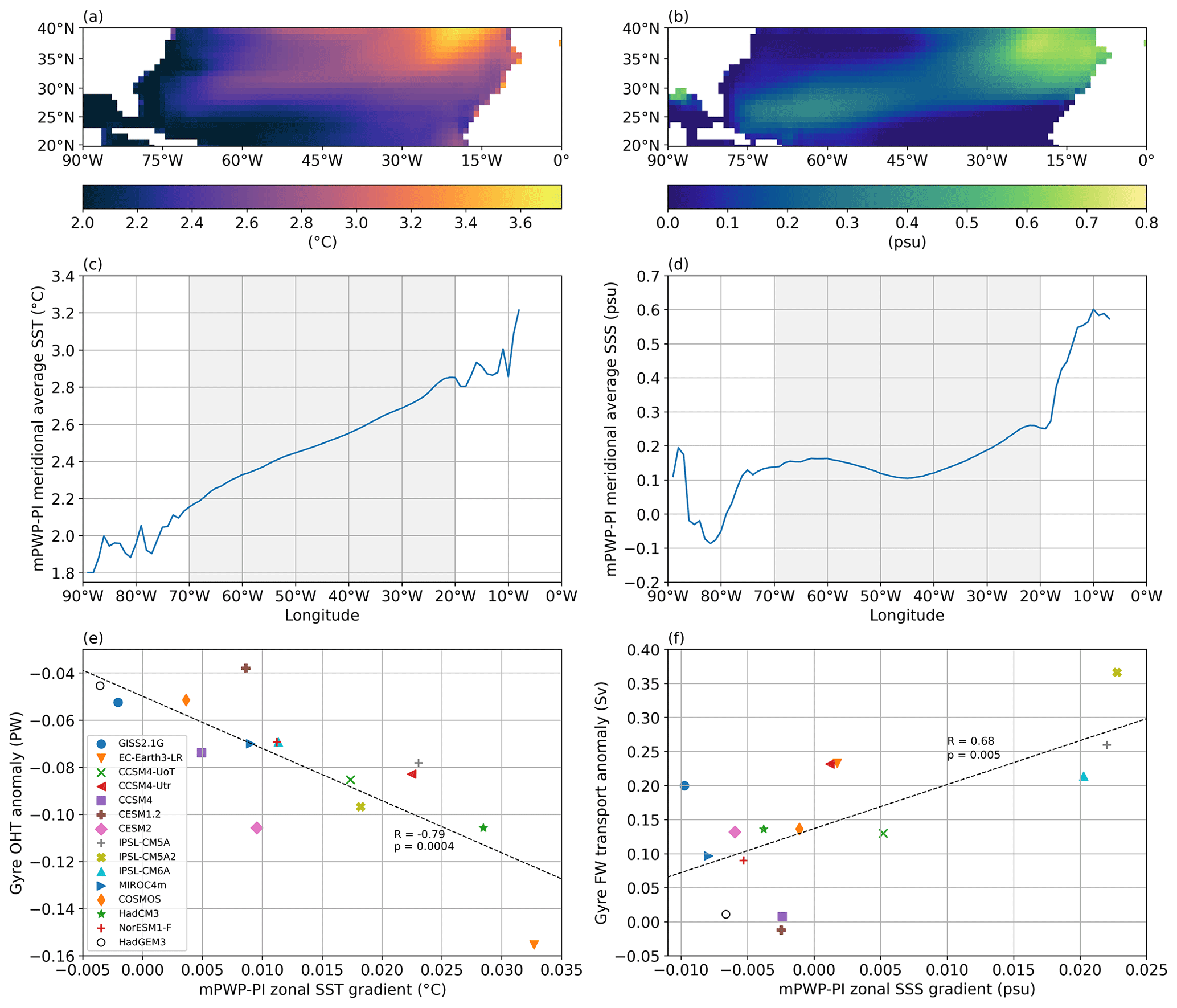
Figure 13 (a) MMM mPWP–PI Atlantic SST difference between 20–40^∘ N. (b) MMM mPWP–PI Atlantic SSS difference between 20–40^∘ N. (c) MMM 20–40^∘ N meridional-mean mPWP-PI Atlantic SST difference. (d) MMM 20–40^∘ N meridional-mean mPWP-PI Atlantic SSS difference. (e) Individual model mPWP–PI mean difference in zonal SST gradient from (c) between 20–70^∘ W plotted against the mPWP–PI difference in the OHT gyre component. (f) Individual model mPWP–PI mean difference in the zonal SSS gradient from (d) between 20–70^∘ W plotted against the mPWP–PI difference in the gyre freshwater transport.

4 Discussion

While there is no consistent relationship between the AMOC strength and average North Atlantic SST warming (Z. Zhang et al., 2021), the correlation maps (Figs. 3 and S2) illustrate that a stronger mid-Pliocene AMOC exerts a relatively larger influence on North Atlantic SSTs. A subset of the models does not show an increase in correlation in the mid-Pliocene: CCSM4, CESM1.2, CESM2, IPSL-CM6A and HadGEM3. As HadGEM3 uses the same land–sea mask in their mid-Pliocene simulations, the lack of stronger correlation is expected for this model. For the other models, the reason is not so evident. Three out of these four models – CCSM4, CESM1.2 and CESM2 – come from the same model family. CCSM4 and CESM2 also show a relatively small increase in overturning OHT with a stronger mid-Pliocene AMOC compared to the other models, even though their sea surface salinity and gateway transport are in line with ensemble behavior.

The high correlation found between North Atlantic SSTs and the AMOC strength in the mid-Pliocene suggests that there likely is a relationship between the stronger AMOC and the amplified North Atlantic SST warming in the mid-Pliocene in the PlioMIP2 ensemble. However, the effect of the AMOC on North Atlantic SSTs is strongly model-dependent and cannot be simply quantified. Other important factors that may influence the SSTs are atmospheric processes and the presence of sea ice (Zhang et al., 2019), as well as model dynamics. For instance, enhanced vertical mixing has been shown to promote surface temperature anomalies at high latitudes in the Pliocene (Lohmann et al., 2022). These factors vary among the different models (e.g., Fig. S8) and cause a varied response of North Atlantic SSTs to mid-Pliocene boundary conditions and CO₂ increase. However, Burton et al. (2022) show that North Atlantic SSTs in the mid-Pliocene are predominantly driven by changes in geography and ice sheets. As we have shown that the mid-Pliocene AMOC strengthening is related to these boundary conditions, specifically the closure of the Arctic gateways, the amplified warming of North Atlantic SSTs and the intensified AMOC are related.

When considering proxy SST data in the North Atlantic, sites 609, 982, 642 and 907 are specifically of interest as they are closest to above-average MMM SST warming in the North Atlantic (Fig. 2b). Disregarding HadGEM3, there are four models at these sites that consistently show the highest warming: EC-Earth3-LR, CCSM4-Utr, CCSM4-UoT and CESM2 (Fig. 2c). While these models all have a stronger mid-Pliocene AMOC, they do not have another common factor that directly connects this warming to a stronger mid-Pliocene AMOC, such as a large increase in overturning or total OHT or a strong correlation of the AMOC to North Atlantic SSTs. It has however been shown by Haywood et al. (2020) that these four models have the highest Earth system sensitivity (ESS) of the PlioMIP2 ensemble together with CESM1.2. On the other hand, their equilibrium climate sensitivity (ECS) varies, where only CESM2 and CESM1.2 have an ECS that is among the highest in the ensemble. As the ESS takes into account long-term feedbacks from ice sheets and paleogeographic boundary conditions, the relatively high warming in these models, which aligns with the warm reconstructed SSTs at sites 962 and 942, may be related to these feedbacks. This strengthens the argument that the AMOC likely does play a role in the amplified North Atlantic warming, as the strengthening of the mid-Pliocene AMOC is related to the boundary conditions. HadGEM3 showing high warming at sites 642 and 907 is probably related to the fact that its ECS of 5.55 ^∘C (Andrews et al., 2019) is the highest of all PlioMIP2 models. Note that HadGEM3 is not among the warmest models at sites 609 and 982, which we expect are the sites that are impacted most by increased OHT due to a stronger mid-Pliocene AMOC.

The AMOC becomes stronger in almost all mid-Pliocene simulations, despite the above-average warming in the subpolar North Atlantic. In future simulations, ocean warming often leads to a weakening AMOC by inhibiting deepwater formation. In our results we show that the strengthening of the AMOC in the mid-Pliocene is a result of high salinity in the Labrador Sea and subpolar North Atlantic. The high salinity is principally caused by two factors: a decreased freshwater transport into the Labrador Sea due to the closure of the Canadian Archipelago and a decrease in surface freshwater flux. Another factor in the increased salinity could be the absence of sea ice over the Labrador Sea in the mid-Pliocene (Fig. S8). However, we find that the annual sea ice cover does not extend into the Labrador Sea in the pre-industrial for the majority of the models. In addition, the high salinity persists below the sea surface, as shown by the average top 100 m salinity (Fig. S6). This field shows the same pattern as the sea surface salinity, and its mPWP–PI anomaly is of comparable magnitude. Overall, our results support the notion that the high mid-Pliocene (sea surface) salinity in the Labrador Sea and subpolar North Atlantic is related to the closure of the Bering Strait and Canadian Archipelago, through both the freshwater transport and the effects on the surface freshwater flux.

The model response of the total Atlantic Ocean heat transport to a stronger mid-Pliocene AMOC is diverse: not all PlioMIP2 models that simulate an intensified AMOC also show enhanced Atlantic OHT in the mid-Pliocene. The opposing response of OHT by overturning and OHT by the gyre in the subtropical gyre region is very likely to be an important cause of this diversity, where individual model dynamics govern the degree to which the two components compensate each other's increase or decrease. However, when considering the overturning component only, all of the models that have a stronger mid-Pliocene AMOC show stronger associated OHT.

It appears that the opposing response of the subtropical gyre OHT component does not result from coupling between the atmospheric forcing of the gyre circulation and the reduced meridional temperature gradient over the mid-Pliocene Atlantic Ocean. Such a mechanism has been proposed by earlier studies such as Farneti and Vallis (2013). As there are no substantial changes in the gyre circulation itself, we find that the (zonal) changes in ocean temperature and salinity fields are responsible for altering the OHT and freshwater transport by the subtropical gyre. We observe that between 20 and 40^∘ N, the eastern part of the Atlantic basin becomes relatively warmer and saltier than the western part in the mid-Pliocene. This results in the gyre circulation transporting relatively more heat and salt southwards than in the pre-industrial. The relatively high temperature and salinity in the eastern subtropical North Atlantic appear to originate from the even warmer and saltier mid-Pliocene subpolar North Atlantic, features that we have related to the stronger AMOC and Arctic gateway closure, respectively. The warm and salty water in the subpolar North Atlantic is transported eastwards by the northern branch of the subtropical gyre and subsequently transported southwards, resulting in the zonal asymmetry we observe. It is possible that the weakened subpolar gyre circulation plays a role in increased eastward transport of the warm and salty subpolar North Atlantic water.

Our results point to a mechanism of compensation between the OHT components in the subtropical gyre region in the Atlantic Ocean. This compensation is, however, not via the atmosphere, as has previously been suggested to be the case in the pre-industrial (Vallis and Farneti, 2009; Farneti and Vallis, 2013). Rather, our results for the mid-Pliocene indicate that the enhanced warming in the mid-Pliocene subpolar North Atlantic SSTs causes more eastward and subsequent southward heat transport by the subtropical gyre. This suggests that the mid-Pliocene background state may affect OHT dynamics and thereby highlights potential differences between the mid-Pliocene and near-future climate. We do not observe such a compensating mechanism in the overturning and gyre components of the freshwater transport.

5 Conclusions

In our study, we have employed 15 models from the PlioMIP2 ensemble to investigate what drives the stronger AMOC in the mid-Pliocene simulations and how the Atlantic OHT and North Atlantic SSTs respond to this strengthening. All models that simulate a stronger mid-Pliocene AMOC show that the closure of the Bering Strait and Canadian Archipelago in the mid-Pliocene leads to a dramatic decrease in southward freshwater transport into the Labrador Sea. The increased salinity in the Labrador Sea and subpolar North Atlantic, which is related to both the decreased freshwater transport through the Canadian Archipelago and decreased surface freshwater flux over the subpolar North Atlantic, stimulates deepwater formation in these areas, leading to a stronger AMOC. These results are consistent with the conclusions of Otto‐Bliesner et al. (2017), who showed that closing the Bering Strait and Canadian Archipelago in their CCSM4 model led to a stronger mid-Pliocene AMOC due to altered freshwater transport in the Arctic and North Atlantic. We show in this study that the increase in salinity in the high North Atlantic is a consistent feature across the mid-Pliocene simulations in the PlioMIP2 ensemble and can be confidently linked to the stronger mid-Pliocene AMOC.

We show that the response of the total Atlantic OHT to a stronger mid-Pliocene AMOC seems inconsistent among models due to a compensation mechanism between the overturning circulation and wind-driven gyre circulation. When separating the OHT into two components, one driven by the overturning circulation and the other by the wind-driven gyre circulation, we find that the OHT associated with overturning does consistently increase with a stronger AMOC. The OHT associated with the subtropical gyre decreases as a response to ocean temperatures increasing more in the east than in the west of the North Atlantic in the mid-Pliocene. This decrease in gyre OHT partially compensates the higher OHT by overturning in the northern subtropical gyre region. As individual model dynamics are highly variable, the degree of compensation differs among models. However, the mean response is consistent. We argue that the OHT components should be considered separately when evaluating the response of the OHT to a stronger mid-Pliocene AMOC. When doing so, we find that the stronger mid-Pliocene AMOC in the PlioMIP2 ensemble does lead to enhanced Atlantic OHT by the overturning circulation.

It has been suggested that the improved data–model agreement in the North Atlantic may be due to a stronger AMOC transporting more heat to the North Atlantic in the PlioMIP2 ensemble (Haywood et al., 2020). Indeed, our results show that the AMOC has a stronger influence on North Atlantic SSTs in the mid-Pliocene than in the pre-industrial. However, the spatial extent and magnitude of this effect are highly variable among individual models, which may explain why Z. Zhang et al. (2021) were not able to identify a consistent relationship between the AMOC strength and average North Atlantic SST warming. It remains difficult to quantify the extent of the influence of the AMOC on North Atlantic SSTs, but our study shows that its influence is significant. Furthermore, we conclude that the AMOC is an important factor in explaining the better agreement of the PlioMIP2 ensemble SSTs with reconstructions in the North Atlantic.

The results presented in this study provide an in-depth look at how the stronger mid-Pliocene AMOC in PlioMIP2 is driven and what its consequences are for the OHT and SST warming in the North Atlantic. They also raise further questions, such as the degree to which the decrease in OHT by the gyre circulation is a response to the increase in OHT by the stronger Atlantic overturning circulation and how the ECS and ESS of individual models may influence modeled SST warming in the mid-Pliocene. Furthermore, given the influence of the stronger mid-Pliocene AMOC on the Atlantic OHT and enhanced SST warming, it raises the question as to what extent and in which context the mid-Pliocene is suitable as a future climate analog. The impact of a stronger AMOC on the regional and global climate is significant and must be taken into consideration when comparing the mid-Pliocene climate to future warming scenarios.