Causes of the weak emergent constraint on climate sensitivity at the Last Glacial Maximum

The use of paleoclimates to constrain the equilibrium climate sensitivity (ECS) has seen a growing interest. In particular, the Last Glacial Maximum (LGM) and the mid-Pliocene warm period have been used in emergent-constraint approaches using simulations from the Paleoclimate Modelling Intercomparison Project (PMIP). Despite lower uncertainties regarding geological proxy data for the LGM in comparison with the Pliocene, the robustness of the emergent constraint between LGM temperature and ECS is weaker at both global and regional scales. Here, we investigate the climate of the LGM in models through different PMIP generations and how various factors in the atmosphere, ocean, land surface and cryosphere contribute to the spread of the model ensemble. Certain factors have a large impact on an emergent constraint, such as state dependency in climate feedbacks or model dependency on ice sheet forcing. Other factors, such as models being out of energetic balance and sea surface temperature not responding below −1.8 ^∘C in polar regions, have a limited influence. We quantify some of the contributions and find that they mostly have extratropical origins. Contrary to what has previously been suggested, from a statistical point of view, the PMIP model generations do not differ substantially. Moreover, we show that the lack of high- or low-ECS models in the ensembles critically limits the strength and reliability of the emergent constraints. Single-model ensembles may be promising tools for the future of LGM emergent constraint, as they permit a large range of ECS and reduce the noise from inter-model structural issues. Finally, we provide recommendations for a paleo-based emergent constraint and notably which paleoclimate is ideal for such an approach.

1 Introduction

The long-term global mean surface temperature response of the Earth to a doubling of atmospheric CO₂ from pre-industrial conditions, referred as equilibrium climate sensitivity (ECS), is an important metric in constraining future climate change (e.g., Forster et al., 2021; Huusko et al., 2021). However, the estimated range of ECS, particularly its upper bound, has been the subject of debate for more than a century (Arrhenius, 1896). In recent years “emergent constraints”, the building of statistical relationships between two variables of the climate system existing in an ensemble of climate models, allowing us to infer one by observing the other, have been extensively used (e.g., Covey et al., 2000; Hall and Qu, 2006). In particular, the possibility of constraining climate properties that are difficult or impossible to measure or observe, such as ECS, makes emergent constraints a powerful tool. Several paleoclimates have a large forcing and temperature anomaly compared to pre-industrial conditions and subsequently receive growing interest for such emergent-constraint analyses (Crucifix, 2006; Hargreaves et al., 2007; Hargreaves and Annan, 2009; Hargreaves et al., 2012; Schmidt et al., 2014; Hopcroft and Valdes, 2015; Hargreaves and Annan, 2016; Renoult et al., 2020). Other methods have calculated ECS by estimating temperature and radiative forcing from the proxy record, such as $\mathrm{ECS}=\frac{\mathrm{\Delta }{T}_{\mathrm{LGM}}}{\mathrm{\Delta }R}\times F_{\mathrm{2}\times {\mathrm{CO}}_{\mathrm{2}}}$, where ΔT_LGM refers to the temperature difference between the Last Glacial Maximum (LGM) and pre-industrial state and ΔR refers to the difference in radiative forcing, including greenhouse gas forcing, ice sheet forcing and sometimes mineral dust forcing (e.g., PALAEOSENS Project Members, 2012; Sherwood et al., 2020; Tierney et al., 2020). The emergent-constraint theory differs from this approach by providing more transparency on the role of global climate models and takes into account the state dependency as simulated by climate models.

Two paleoclimate events particularly stand out within emergent-constraint frameworks: the Last Glacial Maximum (23–19 kyr ago, hereafter LGM) and the mid-Pliocene warm period (3.29–2.97 Myr ago, hereafter Pliocene). The LGM represents peak conditions at the last glacial period with a maximum extent of sea ice and ice sheets, minimum greenhouse gas concentrations, and high atmospheric loading of dust particles, leading to an estimated radiative forcing of −6.8 W m⁻² (−9.6 to −5.2 W m⁻², 95 % confidence interval (Tierney et al., 2020)). By contrast, the Pliocene is a warm paleoclimate with a continental configuration and greenhouse gas concentrations close to modern times, which make the Pliocene a potential analog of future climates (Dowsett et al., 2009; Haywood et al., 2011). The LGM was one of the initial focus periods of the Paleoclimate Modelling Intercomparison Project (PMIP) Phase 1 (Joussaume and Taylor, 1995), and more than 40 models have simulated the LGM through the four generations of PMIP. The LGM has a relative abundance of proxy data as a result of its proximity to the present day, and a large forcing signal and reconstructed LGM temperatures are better constrained than those for the Pliocene. However, despite the LGM being a more promising candidate for a temperature-based constraint on ECS than the Pliocene, studies using the tropical LGM temperatures have estimated a wider range and a higher upper bound of ECS (0.6–5.2 K, 90 % interval) than from the Pliocene (0.5–4.4 K, 90 % interval) (Renoult et al., 2020).

As ECS is defined by global mean temperature, one can argue that in general a model with higher ECS should generate a cooler LGM global temperature than a model with lower ECS. However, previous studies have reported a weak correlation between global LGM temperature and ECS (Crucifix, 2006; Hargreaves et al., 2012), and the more robust constraints were based on tropical LGM temperature (Hargreaves et al., 2012; Schmidt et al., 2014; Hopcroft and Valdes, 2015; Renoult et al., 2020). Using the latter has the advantage of mitigating the large effect of extratropical non-CO₂ forcing, namely the Northern Hemisphere ice sheets or the Antarctic ice sheets. In addition, the coverage in geological proxy data at the LGM is generally good in the tropics (e.g., Tierney et al., 2020) and until PMIP2, most of the spread in ECS was driven by the spread in tropical climate feedbacks (Bony et al., 2006; Webb et al., 2006).

Since PMIP3, the strength of the LGM emergent constraint has decreased considerably compared to its Pliocene counterpart. Another disadvantage is that the spread of tropical temperatures within climate models at the LGM is smaller than the spread in global temperatures, owing to the larger amplitude of LGM polar temperatures. For example, Renoult et al. (2020) showed a tropical temperature spread of around 2 ^∘C in the whole PMIP ensemble, while Hargreaves et al. (2012) had a spread of more than 3.5 ^∘C in the global temperature of the PMIP2 ensemble. A narrow range is an issue for emergent-constraint analysis, as it renders statistical methods more sensitive to outliers and noise. In this study, we define noise as the uncertainty arising from climate physics in the ensemble of models which impacts the statistical relationship, potentially different from a systematic bias. In Fig. 1, we show that the relationship from the global constraint is nonexistent at the LGM after PMIP3, while the Pliocene constraint can be regarded as robust across the model generations. The reasons suggested for a weaker LGM constraint can be summarized as follow:

• Structural differences in LGM simulations. Despite more models simulating the LGM, Hopcroft and Valdes (2015) suggested that differences in model evolution and in particular the additions of dynamical vegetation and aerosol-related effects were enough to generate discrepancies between PMIP generations. This would affect LGM models more as these span four generations of models, whereas the Pliocene spans only the two most recent generations of models. Whilst the argument of Hopcroft and Valdes (2015) is reasonable, we show in this paper that this explanation alone is insufficient. Notably, models are suspected of being out of equilibrium at the LGM as well as having various representations of ice sheet forcing, ocean circulation and snow-albedo feedbacks.

• State dependency between LGM and abrupt4×CO₂. Because the LGM is a cold climate, feedbacks may behave differently compared to a warmer climate. This state dependency usually leads to model-based estimates of ECS from LGM temperature being lower than from 4×CO₂ experiments (PALAEOSENS Project Members, 2012; von der Heydt et al., 2014). We show in this study that several aspects of the climate are affected differently between cooling and warming climates and could weaken the relationship between the LGM and future climate change. Specifically, cloud, albedo and water vapor feedbacks may differ in strength between the LGM and the abrupt4×CO₂ state from which the ECS is computed.

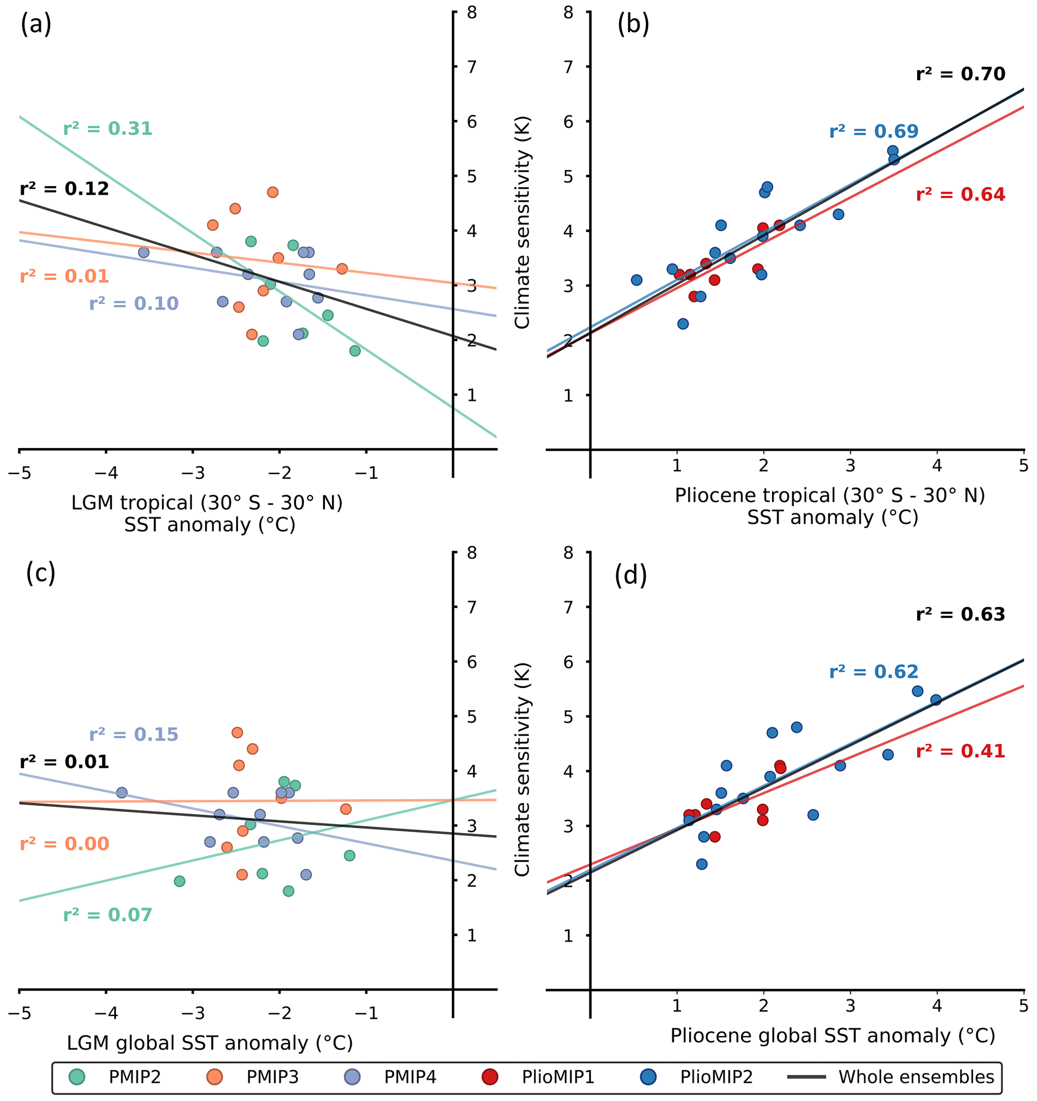
Figure 1 Emergent constraints for the LGM (a) tropical and (c) global SST anomaly and the ECS of PMIP2, PMIP3 and PMIP4 models. Emergent constraints for the Pliocene (b) tropical and (d) global SST anomaly from PlioMIP1 and PlioMIP2 models. Ordinary least squares regression is calculated, and the coefficients of determination r² from each sub-ensemble is shown to illustrate the quality of the regression. For the LGM, CESM2.1 is filtered out as discussed in Sect. 6.

The aim of this paper is to provide a framework for the future development of paleo-emergent constraints by addressing the following question: why are the LGM regional and global constraints weakly correlated with ECS compared to the Pliocene constraint?

The paper is organized as follows:

• Sect. 2 – we define the climate sensitivity, temperature variable and emergent-constraint theory. We describe the PMIP models and the ensemble of analysis performed to investigate the spread of models.

• Sect. 3 – we extend on methodological considerations by analyzing global and regional correlations between temperatures and ECS in the LGM ensembles so as to provide a better view on potential tropical and extratropical biases.

• Sect. 4 – we show the different aspects of the climate system which can be suspected as significant contributors of noise in the emergent constraints. This considers several climate components, i.e., atmosphere, ocean, land surface and cryosphere.

• Sect. 5 – we discuss the results of Sect. 4, in particular the contribution and amplitude of noise in the emergent-constraint relationship arising from the LGM-modeled climate. We categorize the sources of noise as state-dependent or structural.

• Sect. 6 – we further discuss issues of the LGM ensemble which are not be directly connected to the physics of the LGM, such as the effect of outlier models and differences between PMIP generations.

• Sect. 7 – we investigate the current potential of single-model ensembles in emergent constraints on ECS by analyzing perturbed physics ensembles of the Max Planck Institute Earth System Model version 1.2 (MPI-ESM1.2-LR), the Community Earth System Model version 2.1 (CESM2.1) and the CESM model family.

• Sect. 8 – we provide further recommendations on using paleoclimates to constrain ECS. We reflect on the biases affecting the LGM constraint and evaluate which past climate is ideal for the emergent-constraint approach.

2 Methodological consideration

In this section, we summarize how paleo-emergent constraints on ECS have been defined within the literature as well as discussing the use of surface air temperature (SAT) and sea surface temperature (SST). We describe the PMIP ensembles since PMIP1 and the two models used for feedback analysis and single-model ensembles: MPI-ESM1.2-LR and CESM2.1. We also detail the sampling and resampling methods applied in Sects. 3 and 6.

2.1 Definition of the emergent constraint

The emergent-constraint approach in its simplest form is a statistical relationship between two climate variables, where one is predicted and the other an observed predictor. In most cases, the predicted variable is difficult to measure or observe, either because it is an idealized metric such as ECS or an outcome in the future (e.g., future sea-ice change; Boé et al., 2009). In this paper, the two variables of interest are the temperature of the LGM and the ECS of climate models. In previous studies, temperature and ECS have been interchanged, with ECS appearing as both the predicted variable (e.g., Hargreaves et al., 2012; Schmidt et al., 2014) and the predictor variable (Renoult et al., 2020). Following the definition of an emergent constraint as a simple linear relationship, the former can be written as Eq. (1) and the latter as Eq. (2).

$$\begin{array}{}\text{(1)}& {\displaystyle }& {\displaystyle }\mathrm{ECS}=\mathit{\gamma }\times T+\mathit{\delta }+\mathit{\zeta }\text{(2)}& {\displaystyle }& {\displaystyle }T=\mathit{\alpha }\times \mathrm{ECS}+\mathit{\beta }+\mathit{ϵ}\end{array}$$

Both Eqs. (1) and (2) are defined with slopes γ and α and intercepts ζ and β, which are obtained by regressing ECS over temperature or vice versa. The parameters ζ and ϵ usually follow a normal distribution N(0, σ²) and represent uncertainty arising in the regression from the spread of the model ensembles. The parameters ζ and ϵ are of particular interest for our study, as they are connected to the aspects of the climate which contribute to the noise of the LGM emergent constraint. It is also possible to add an uncertainty parameter dependent of the predicted variable (i.e., on the left-hand side of Eqs. 1 or 2) and certain statistical methods, such as orthogonal distance regression, take into accounts errors in both predicted and predictor and have been used in other emergent-constraint analyses (Jiménez-de-la Cuesta and Mauritsen, 2019).

It is debated which statistical method is best applied in emergent-constraint frameworks. However, the noise existing in an ensemble of models is independent of the choice of statistical approach used to infer ECS, as models are not built to be related by specific statistical relationships. The Pearson correlation coefficient arising from the relationship between the LGM temperatures and ECS is also independent of the choice of Eqs. (1) or (2) as it is symmetrical. Therefore, discussions regarding statistical methods are beyond the scope of this study, but we provide ECS estimates when discussing single-model ensembles in Sect. 7.

Both SAT (Hargreaves et al., 2012; Renoult et al., 2020) and SST (Hargreaves and Annan, 2016; Renoult et al., 2020) have been used in emergent-constraint studies. From a geological point of view, marine proxies are more abundant than land-based proxies, and so using SST is more meaningful. For the LGM, there is relatively good coverage of land proxies (Cleator et al., 2020), in contrast to the Pliocene, which creates the potential for using either land-only or all-surfaces temperatures. However, ECS values are often computed from SAT in models (e.g., Andrews et al., 2012), which can lead to differences with other temperature variables. For example, MPI-ESM1.2-LR has an ECS reported as 2.77 K in PMIP4 (Kageyama et al., 2021) based on surface temperature, while Mauritsen et al. (2019) showed an ECS of 3.01 K using SAT. SAT is extrapolated and amplified by surface temperature in climate models, whereas observations show the opposite (Gulev et al., 2021). Thus, one could expect emergent constraints using SAT to be inherently biased by this disagreement. In the case of SST, there is little difference between SST and surface temperature for a large part of the globe. In polar regions, discrepancies between the two can be found due to the presence of sea ice, and it is shown later to influence the correlation between polar temperatures and ECS.

There is ambiguity in the definition and calculation of climate sensitivity in climate models. In this paper and unless specifically noted, ECS refers to the methodology of Gregory et al. (2004), an approximation of the long-term equilibrium climate sensitivity from 150-year-long perturbed experiment, as it is commonly adopted by the community. However, other studies have used the broader S as “sensitivity” (Hargreaves et al., 2012; Schmidt et al., 2014; Renoult et al., 2020), and some of the ECS estimates of PMIP1 and PMIP2 models were computed from slab ocean experiments (Hargreaves et al., 2012; Hopcroft and Valdes, 2015). It is possible that differences in emergent constraints arise from these ambiguities. However, we do not explore this further.

2.2 Variables and models analyzed

The climate variables analyzed for each model in this study are summarized in Table 1. PMIP spans 3 decades and the models used to simulate the LGM in PMIP1 and PMIP2 were considerably less complex than more recent models. PMIP1 models were typically atmospheric general circulation models (AGCMs) with low resolution and limited representation of land surfaces and vegetation. For PMIP2, all models except ECBILTCLIO were atmosphere–ocean general circulation models (AOGCMs). By PMIP3, a few models started to include complex processes like dynamical vegetation and aerosol–cloud interactions (Hopcroft and Valdes, 2015), while the majority of the models of PMIP4 have implementations of those components.

Kattenberg et al. (1996)Meehl et al. (2000)Ganopolski et al. (2001)Thompson and Pollard (1995)Thompson and Pollard (1997)Kattenberg et al. (1996)Gallée et al. (1992)Treut et al. (1994)Cubasch et al. (2001)Kattenberg et al. (1996)Hopcroft and Valdes (2015)Hopcroft and Valdes (2015)Hopcroft and Valdes (2015)Hopcroft and Valdes (2015)Hopcroft and Valdes (2015)Hopcroft and Valdes (2015)Hopcroft and Valdes (2015)Hopcroft and Valdes (2015)Kageyama et al. (2021)Kageyama et al. (2021)Kageyama et al. (2021)Kageyama et al. (2021)Kageyama et al. (2021)Kageyama et al. (2021)Kageyama et al. (2021)Kageyama et al. (2021)Kageyama et al. (2021)Kageyama et al. (2021)Kageyama et al. (2021)Kageyama et al. (2021)Kageyama et al. (2021)Kageyama et al. (2021)Kageyama et al. (2021)Zelinka et al. (2020)Kageyama et al. (2021)Kageyama et al. (2021)Kageyama et al. (2021)Kageyama et al. (2021)

Table 1 Summary of the models used in this study and their components. Clim. refers to climatological means. SSTs are reported as tropical (30^∘ S–30^∘ N) anomalies from pre-industrial conditions. ^* When compared to other versions of the CESM model family, the ECS of 5.6 K from abrupt2×CO₂ in the slab ocean mode of Zhu et al. (2021) is used.

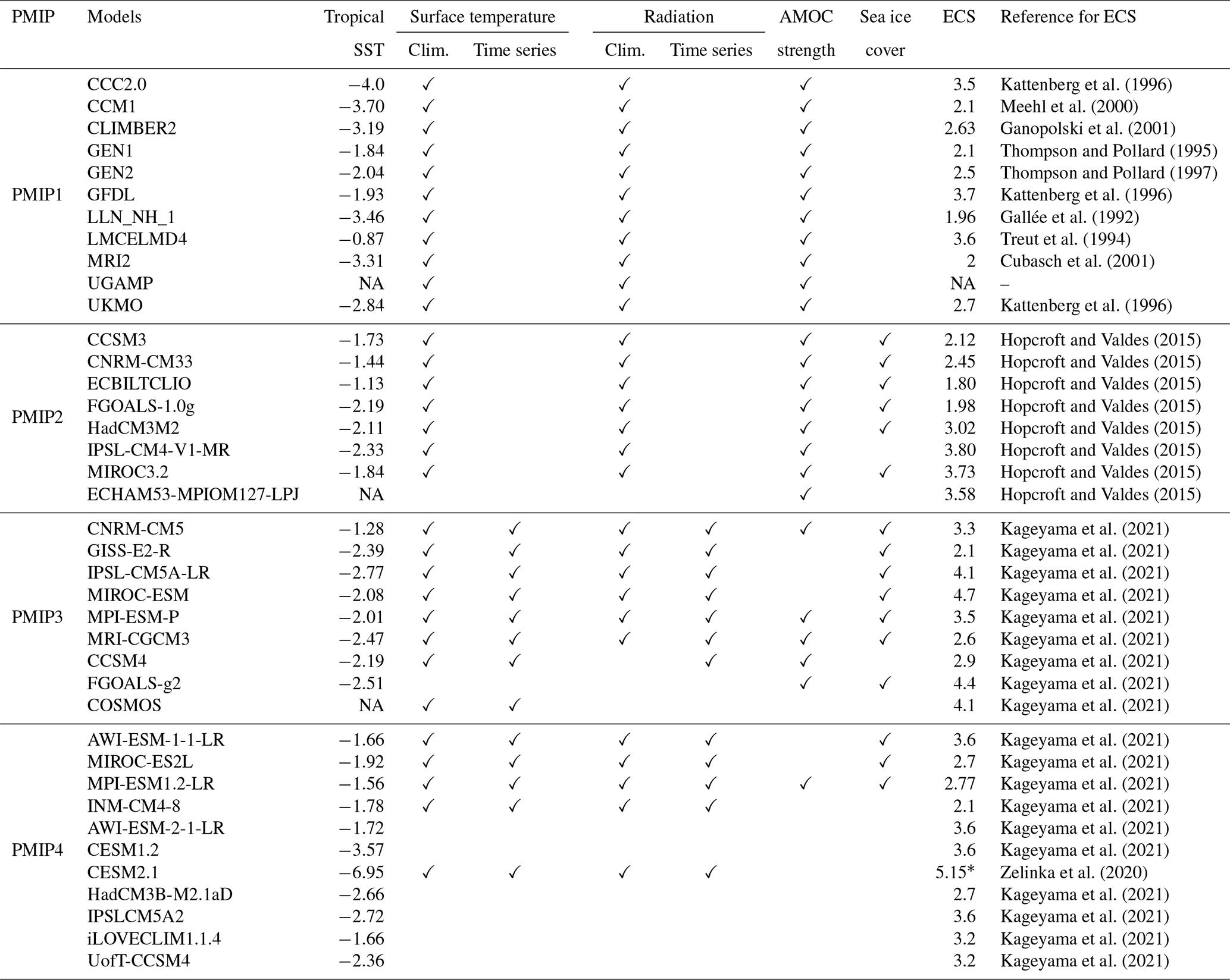
NA stands for not available.

The availability of the data is based on the current state of each PMIP database, which differs notably from the studies of Hargreaves et al. (2012), Hargreaves and Annan (2016), or Renoult et al. (2020), as models have been removed or added over time. For PMIP4, which is still ongoing at the time of writing, only SSTs were available to be examined for the majority of the models. We have also included several model variants as they can provide information on the sensitivity of the climate system to specific components. Notably we included the following: p151 of GISS-E2-R, which has a different ice sheet mask than other PMIP3 models (“Laurentide enhanced”); p2 of MPI-ESM-P, which has dynamical vegetation enabled as opposed to the p1; and variants of iLOVECLIM1.1.4 using the ice sheet mask GLAC-1D and of HadCM3B-M2.1aD using the mask GLAC-1D and the PMIP3 mask (blending of ICE-6G, GLAC-1a and ANU), whereas the most commonly used mask is ICE-6G_C within PMIP4 (Kageyama et al., 2021). We exclude the variants from emergent-constraint and correlation analyses, similarly to previous studies, but include them in SSTs or effective albedo analyses, as their behavior can be indicative of structural uncertainties existing in the ensemble.

PMIP1 models were omitted in previous LGM emergent-constraint studies. This is due to a number of reasons: PMIP1 models were AGCMs and most of them had prescribed SSTs or ran slab ocean experiments only (Joussaume and Taylor, 1995); their resolutions are low compared to modern standards (e.g., Williamson et al., 1987; Thompson and Pollard, 1997); there are substantial differences in boundary conditions compared to other PMIPs, such as particularly lower ice sheets (Peltier, 1994) and an independent definition of non-CO₂ trace gases (Joussaume and Taylor, 1995); the ECS of PMIP1 models and likewise details of the methods, notably length of integration, are difficult to find. The comparison of ECS of PMIP1 models to PMIP2, PMIP3 and PMIP4 models is therefore challenging. Finally, most of the variables analyzed in our study are not available for PMIP1 models. Thus, we focus our analyses on PMIP2, PMIP3 and PMIP4, but results from PMIP1 are explored in Sect. 6.

2.3 Simulation of LGM climate

2.3.1 Partial radiative perturbation

We use the coupled model MPI-ESM1.2 at a low resolution (∼2^∘, MPI-ESM1.2-LR) (Mauritsen et al., 2019) to investigate aspects of the LGM climate in this study. MPI-ESM1.2-LR contributed to the Climate Modelling Intercomparison Project Phase 6 (CMIP6) and PMIP4, and its predecessors were present in all generations of PMIP since PMIP1. MPI-ESM1.2-LR matches the warming observed since the pre-industrial period well (Mauritsen and Roeckner, 2020) as well as reconstructions of the LGM SSTs but is found to be too warm compared to LGM land temperature reconstructions (Kageyama et al., 2021).

To perform climate feedback analysis, we used an online module of partial radiative perturbation (PRP) in ECHAM6.3. The method has been described by Wetherald and Manabe (1988) and Colman and McAvaney (1997), and its implementation in ECHAM was carried out in Meraner et al. (2013). The PRP method exchanges variables of surface albedo, clouds, humidity and temperature between a stored control state and the current state of interest and calculates the influence on top-of-atmosphere (TOA) fluxes arising from each component. In this study, we were interested in exchanging cloud-related properties between control (LGM and pre-industrial states) and abrupt CO₂ doubling and halving experiments as well as albedo and water vapor radiative properties in order to evaluate the strength of the climate feedbacks in the model under conditions different from pre-industrial ones.

From pre-industrial conditions, we ran simulations for 150 years with instantaneous and sustained doubling (abrupt2×CO₂) and halving (abrupt0p5×CO₂) of CO₂ concentrations, following the protocol of Webb et al. (2017). The runs were compared to a control pre-industrial run of the same length. In the case of our LGM simulation, we ran it for 150 years continuing from the spun-up LGM simulations (Marie-Luise Kapsch, personal communication, 2019), which follow the PMIP4 protocol of Kageyama et al. (2017). The latter includes changes in ice sheet masks and reduced greenhouse gas concentrations compared to PMIP3. From that state, we abruptly doubled the LGM CO₂ concentration, ran it for an additional 150 years and compared it to the control LGM state to estimate the climate feedbacks.

2.3.2 Perturbed physics ensembles

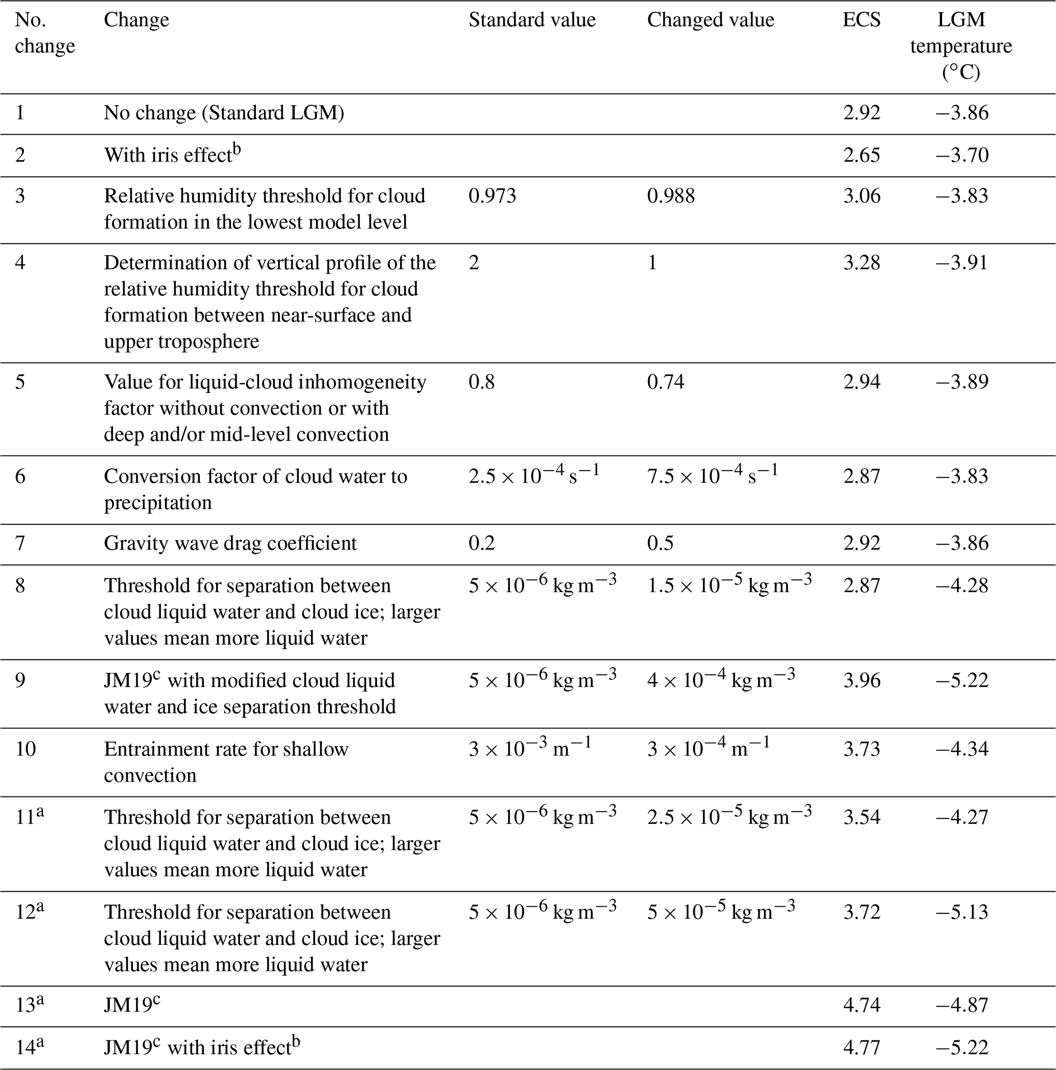
In addition to the PMIP LGM ensemble, we use two single-model ensembles from MPI-ESM1.2-LR and CESM2.1 as well as an ensemble of the CESM model family. For MPI-ESM1.2-LR, we explore 14 LGM simulations where parameters which have a large impact on cloud feedbacks and climate sensitivity were perturbed in order to create an ensemble with a range of ECS values from 2.7 to 4.8 K (Sagoo, 2023). Pre-industrial, abrupt4×CO₂ and LGM simulations were run for 150 years or until the simulations crashed. The 150 years of the pre-industrial and abrupt4×CO₂ simulations were used to calculate ECS using linear regression (Gregory et al., 2004). The LGM simulations were branched from the equilibrated PMIP4 LGM contribution from the Max Planck Institute, Hamburg (Marie-Luise Kapsch, personal communication, 2019). The description of the 14 runs is in Table 2. The MPI-ESM1.2-LR single-model ensemble is compared to the single-model ensemble made of perturbed cloud physics versions of CESM2.1 (Zhu et al., 2022a), spanning the range of ECS of 3.7–6.1 K, calculated using abrupt2×CO₂ in slab ocean model configuration.

Table 2 Summary of the simulations of the single-model ensemble of MPI-ESM1.2-LR. ^a Unstable runs, where the temperature is an estimate of the last 50 years before numerical crash. ^b Iris effect implementation of Mauritsen and Stevens (2015). ^c JM19 refers to runs with all the changes in the table as well as an increase in the relative humidity threshold for cloud formation at high model level, a decrease in entrainment rate in shallow convection and a decrease in minimum excess buoyancy, as described by Jiménez-de-la Cuesta and Mauritsen (2019).

Additionally, we compare this to the six-member ensemble of different configurations of CESM1.2 and CESM2.1. These coupled simulations have been run to quasi-equilibrium, making this smaller ensemble valuable. This ensemble uses CESM1.2 with CAM5 at a ∼2^∘ resolution (Zhu and Poulsen, 2021), CESM1.3 with CAM5 at a ∼2^∘ resolution (Zhu et al., 2017), CESM2.1 with CAM6 at a ∼1^∘ resolution (Zhu et al., 2021), CESM2.1 with CAM5 at a ∼1^∘ resolution (Zhu et al., 2021), CESM2.1 with CAM6 at a ∼1^∘ resolution and the CAM5 ice nucleation scheme (Zhu et al., 2022a), and CESM2.1 with paleoclimate-calibrated CAM6 at ∼2^∘ (see Zhu et al., 2022a for details).

2.4 Resampling and sampling methods

The ensemble size of each phase of PMIP is small with an average of 8 models in comparison to PlioMIP2 with 16 models. This has been a limitation in studies focused on individual ensembles (Crucifix, 2006; Hargreaves et al., 2012). There is a risk of identifying relationships which are coincidental in smaller ensembles (Caldwell et al., 2014). Therefore, a high level of correlation is required for a constraint to be meaningful in smaller ensembles. For instance, as only four models were available at that time, Crucifix (2006) would have needed a correlation higher than 0.9 from a 95 % threshold one-sided test of correlation for a significant relationship between SST and ECS in PMIP2 (Hargreaves et al., 2012). Because of those concerns, resampling and sampling methods are of particular interest, as they can provide new insights into the correlations and emergent-constraint relationships.

In this study, we apply one resampling method, the permutation test, and one sampling method, the simple random sampling. For the permutation test, we interchange the sensitivity of PMIP models and generate 10 000 random ensembles to investigate correlation patterns between SST and ECS around the globe, similar to Hargreaves et al. (2012) for the PMIP2 ensemble. This allows us to test whether a pattern is likely to appear by chance, notably as an artifact of small size ensemble. We compute the 5th and 95th percentiles of the distribution of correlation coefficients of each of the 10 000 permuted ensembles at each grid cell, with the models regridded at a 10^∘ resolution to minimize dependency in neighboring cells. If the correlation in the real ensemble is outside of the computed 5 %–95 % interval, then such a correlation is unlikely to happen by chance. Here, we extend on Hargreaves et al. (2012) as we include the ensemble of PMIP3 and PMIP4 in the permutation tests to check if certain patterns would appear in ensembles of 15 to 26 members. These results are explored in Sect. 3.

For the case of simple random sampling, we investigate the creation of smaller sub-ensembles of models from the larger PMIP ensemble by randomly sampling models and generating 100 000 smaller PMIP sub-ensembles. The size of the sub-ensemble is set to eight members, as it is the average size of single-generation PMIP ensembles.

3 Regional correlations

The correlation between SST and ECS at the LGM has important regional and generational disparities. A negative correlation between SST and ECS for the LGM is expected, as it implies models with high ECS would simulate a larger cooling as opposed to models with low ECS (Hargreaves et al., 2012). However, patterns of weak, near-zero or positive correlations can be seen around the globe in most ensembles. This is the opposite of the correlation between ECS and SST in abrupt4×CO₂ simulations, where the correlation is almost globally positively significant (not shown).

We summarize the correlation between SST and ECS at the LGM and the Pliocene among different PMIP generations in Fig. 2. Significance is calculated from a one-sided t test at a 95 % threshold. Correlation maps assume the temperature of cells to be strictly independent of neighboring cells, which is an approximation of reality. Nevertheless, they provide a useful qualitative representations of the sources of noise in the emergent constraint between SST and ECS.

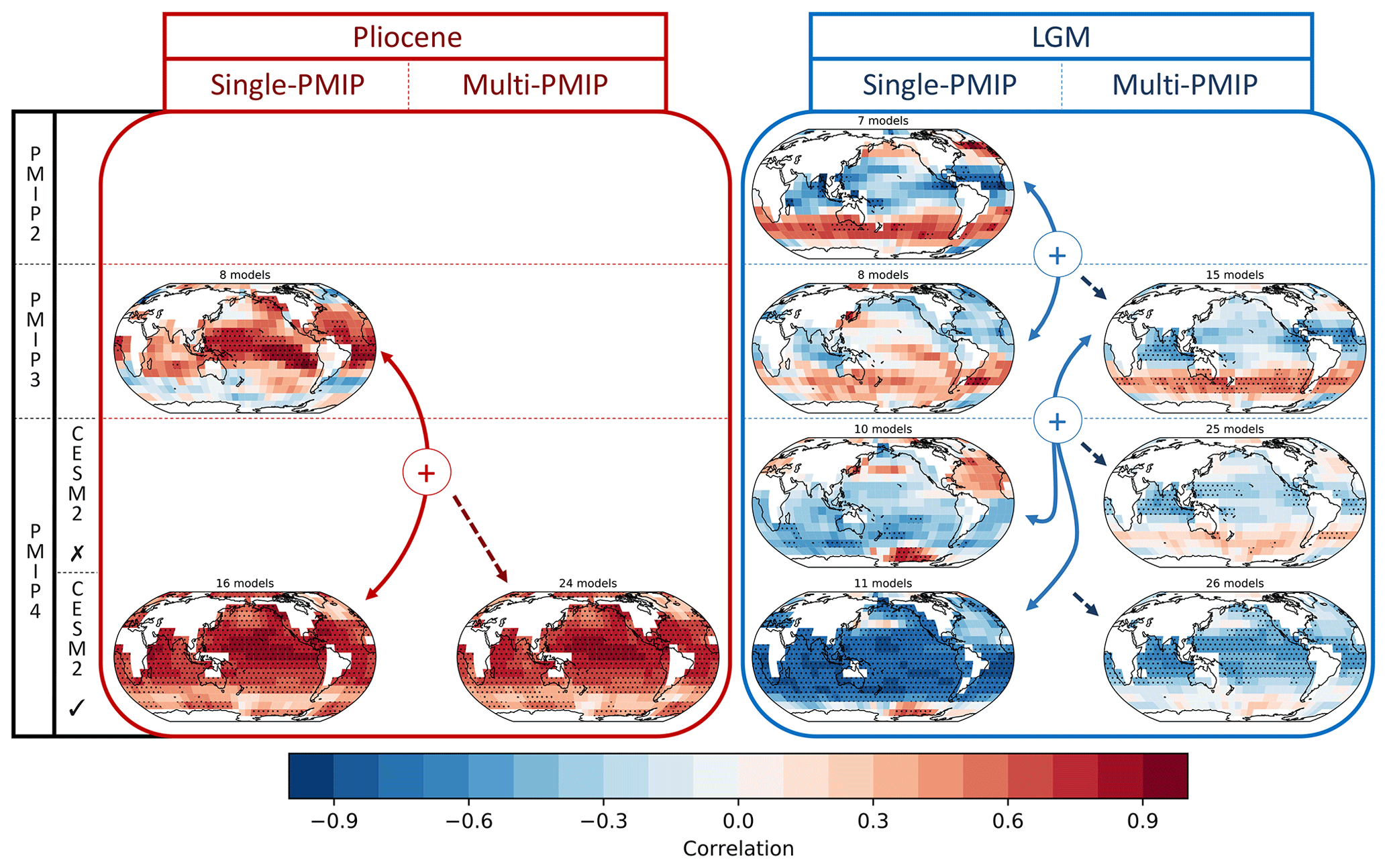
Figure 2 Summary of the correlation between SST anomaly and ECS through different PMIP generations. Models have been regridded on 10^∘ grids to minimize dependency between neighboring cells. For both Pliocene and LGM, the left-hand side figures correspond to the correlation existing in each individual generation of PMIP, while the right-hand side figures are the combination of several generations, following the “+” sign. In PMIP4, the upper row shows ensembles with CESM2.1 included, while lower row shows ensembles excluding CESM2.1. Discussions regarding the presence of CESM2.1 are made in Sect. 6. Red dotted areas are of positive significance; blue dotted areas are of negative significance under a one-sided t test (95 % threshold).

For the Pliocene, the correlation is significant in the tropics in PMIP3 and extends far into the extratropics in PMIP4. Regions with low or negative correlation are the Southern Ocean and the North Atlantic. These patterns of correlation are close to the ones arising from ECS and SST in abrupt4×CO₂ experiments. From these two model generations, emergent constraints between SST and ECS seem robust for the Pliocene.

The evolution of LGM-based emergent constraints is less clear across the generations. In PMIP2, there is a significant negative correlation in the tropics, as expected when correlating cooling temperatures to increasing ECS, and positive correlation in the Southern Ocean. A regional positive correlation means that more sensitive models cool less in those regions in their LGM simulations than low climate sensitivity models. In the PMIP3 ensemble, the patterns are broadly split equally between positive and negative correlation but remain weak and below significance on the correlation map. In PMIP4, the correlation is negative and highly significant in most of the globe when CESM2.1 is included. This is caused by the high ECS and resulting large cooling of CESM2.1, which strengthens the constraint. If CESM2.1 is filtered out, the correlation drops and is insignificant in most parts of the globe.

Interestingly, SST over the northern Atlantic Ocean exhibits a relatively large positive correlation with ECS in LGM simulations. Whether or not CESM2.1 is included in the ensemble, there are significant correlations in the tropics. However, the tropical patterns have a low correlation (minimum of −0.3) when CESM2.1 is not included and the global correlation is close to zero, whereas tropical patterns have a high correlation (close to −0.6) when CESM2.1 is in the ensemble. One could reason that if the robustness of an emergent constraint is based solely on the presence of a single model, the constraint itself may not be reliable or such a single model needs to be considered separately of the ensemble. The value of very low- or high-ECS models, like CESM2.1, is discussed further in Sect. 6.

The presence of near-zero or positive correlations in the Southern Ocean at the LGM is particularly interesting and is seen in most ensembles. The phenomenon was observed in the PMIP2 ensemble (Hargreaves et al., 2012) and is visible in the PMIP3 ensemble and the combination of PMIP2 + PMIP3 (Fig. 2). This unexpected correlation is not unique to the LGM, as it has been observed to a lesser extent during the Pliocene (Fig. 2 and Hargreaves and Annan, 2016) and abrupt4×CO₂ simulations. Hargreaves et al. (2012) suspected the positive correlation to arise from the small size of the PMIP2 ensemble, but its existence in larger ensembles contradicts that hypothesis.

In Fig. 3, we show that from permuted individual PMIP2 and PMIP3 ensembles, the Southern Ocean positive correlation is likely to appear by chance in the real individual PMIP2 and PMIP3 ensembles. However, the combination PMIP2 + PMIP3 leads to a large part of the Southern Ocean positive correlation passing the statistical significance test, indicating that it is unlikely to have such a positive correlation pattern appearing by chance within this 15-model ensemble. Curiously, the Southern Ocean true correlation in PMIP2 + PMIP3 + PMIP4 falls within the permuted ensemble interval, raising the question of whether such a pattern is influenced by PMIP4 models. When CESM2.1 is included, the highly negative tropical correlation of the true PMIP ensemble passes the statistical significance test, indicating it is unlikely to appear by chance. When CESM2.1 is removed, only the tropical Indian Ocean passes the significance test (not shown).

Figure 3 Correlation between SST anomaly and ECS (as in Fig. 2) in (a) PMIP2, (b) PMIP3, (c) PMIP2 + PMIP3 and (d) PMIP2 + PMIP3 + PMIP4 (CESM2.1 included) and comparison to a 10 000-member permuted ensemble. If hatched, the correlation in the real ensemble at that cell is outside the 5 %–95 % interval of the correlation distribution of the permuted ensemble and is thus unlikely to appear by chance. Models have been regridded on 10^∘ grids to minimize dependency between neighboring cells.

Based on the above analysis, the robustness of a relationship between ECS and LGM SST is compromised. We shall argue next that this is caused by numerous sources of noise acting on the relationship between LGM global cooling and ECS. Moreover, the differences in correlation between the extratropics and the tropics may arise from the sources of noise which are essentially extratropically based, which reinforces the use of tropical LGM SST over global SST for emergent constraints.

4 Investigation of LGM climate physics

In this section, we describe and analyze several potential sources of noise and biases which may impact the emergent constraint between LGM temperatures and ECS. This assessment targets all climate components, i.e., the atmosphere, ocean and land surface, but also investigates whether potential biases preferentially affect models individually, through PMIP generations, or the ensemble as a whole. The contribution of each source to the uncertainty of the emergent constraint is given in Sect. 5.

4.1 Temperature drift and energy leakage

Climate models which have not been spun-up sufficiently, i.e., have not been run for the time required for a model to reach its steady state, may experience drift of their climate state. This was shown by Mauritsen et al. (2012) on pre-industrial simulations in the CMIP3 and CMIP5 ensembles where some model pre-industrial simulations would drift as far as 1 ^∘C from their initial temperature within 500 years. Ideally, when in a steady state, climate models would also have a TOA radiation balance at equilibrium, implying that energy is neither created nor lost artificially.

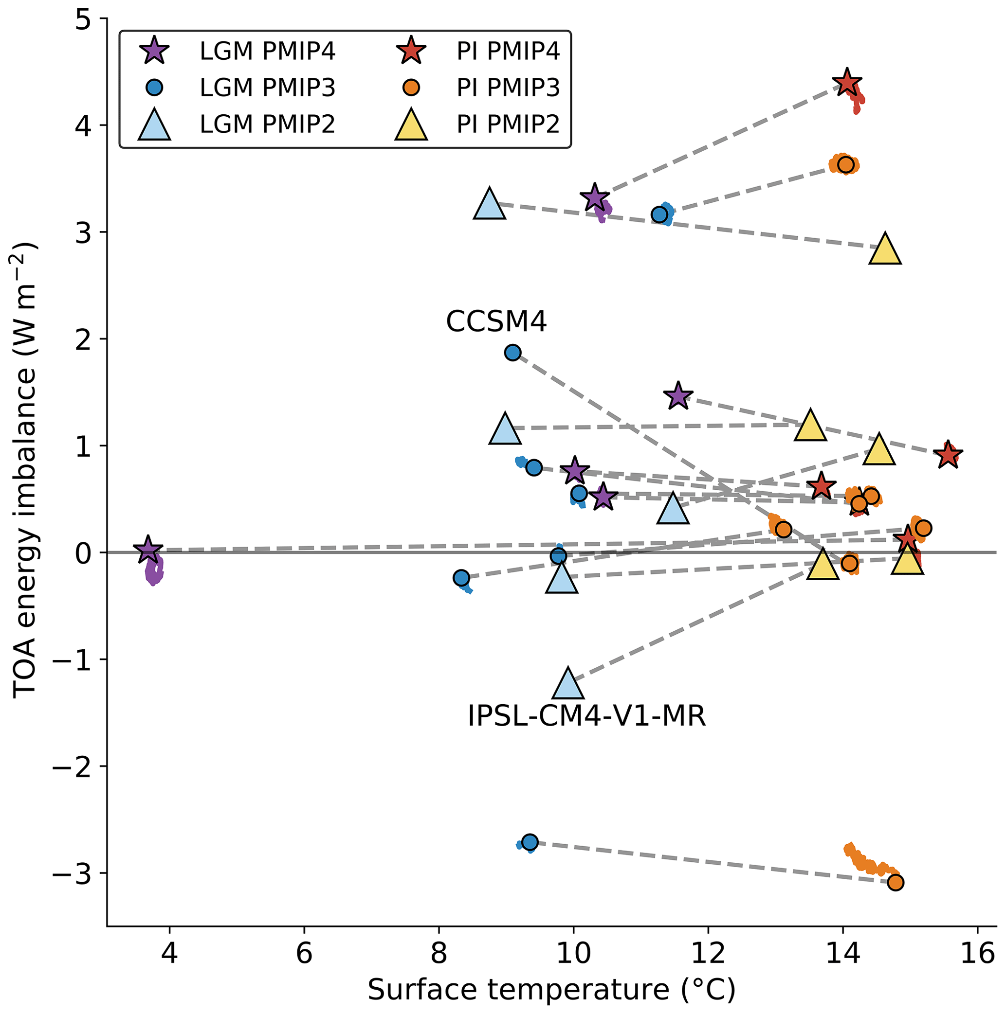
Figure 4 Surface temperature (^∘C) and top-of-atmosphere (TOA) radiation imbalance (W m⁻²) drift in PMIP models simulating LGM (blue scale) and pre-industrial (PI, orange scale) states. Each trail is a 30-year running mean, while the symbol is a mean of the last 30 years of the time series, when applicable. The gray line connects the LGM and piControl simulation of each model. Note that for PMIP2 models and CCSM4 for PMIP3, time series are not available.

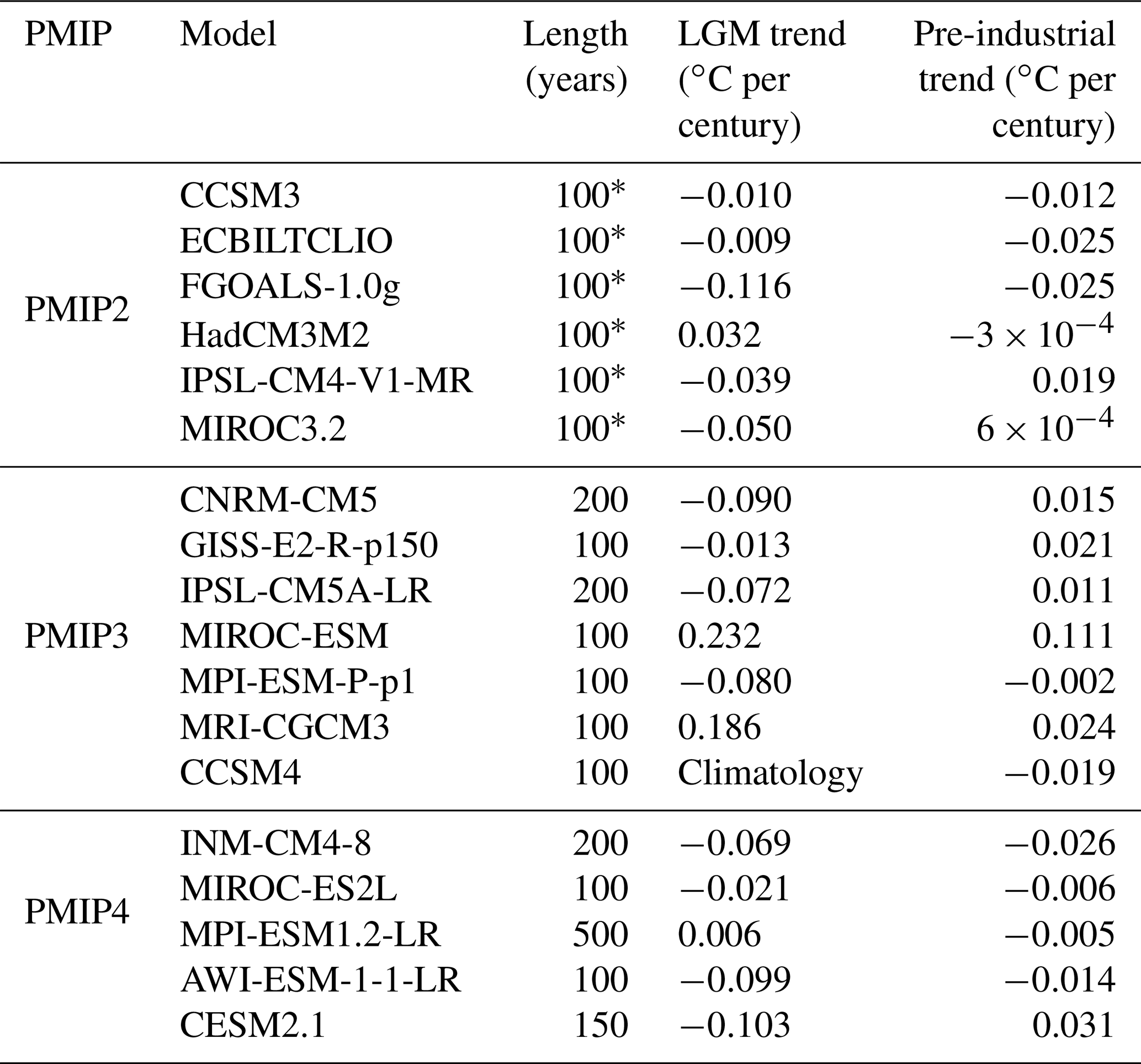
We show the time evolution of surface temperature and TOA imbalance in models simulating the LGM and pre-industrial climates in Fig. 4 and report the drifts of temperature per century in Table 3. As limited computational power was available at the time, PMIP2 models could be suspected to be further out of equilibrium than newer model generations. However, several of them applied acceleration techniques to reach near-equilibrium state, namely forced adjustment of SSTs to glacial SSTs (Haney, 1971; Hewitt et al., 2003) or acceleration of abyssal temperatures (Bryan, 1984; Shin et al., 2003), though for the most parts, details of the spin-up procedures are usually undocumented. In PMIP2, the largest drifts are for FGOALS-1.0g and MIROC3.2, respectively, of −0.116 and −0.050 ^∘C per century (Braconnot et al., 2007). In PMIP3 and PMIP4, most drifts are comprised of between −0.1 and −0.05 ^∘C per century, with two models of PMIP3 standing out: MIROC-ESM and MRI-CGCM3, with drifts of 0.23 and 0.19 ^∘C per century, respectively. This could be connected to the abandonment of acceleration techniques when modeling centers could afford running the ocean models to near-equilibrium. As opposed to FGOALS-1.0g and MIROC3.2, the drifts of MIROC-ESM and MRI-CGCM3 are positive and would indicate a warm-drifting LGM equilibrium temperature, implying that the LGM temperature estimate is low-biased in those models.

Table 3 Temperature trends in degrees Celsius per century for models of PMIP2, PMIP3 and PMIP4. For PMIP2, we report the results of Braconnot et al. (2007). Trends in PMIP3 and PMIP4 models are computed as the difference between the mean of the last 30 years and the mean of the first 30 years, normalized by simulation length. ^* Simulations have a minimum length of 100 years but may be up to 200 years long (Braconnot et al., 2007).

The models CCSM4 and IPSL-CM4-V1-MR appear to be either far from equilibrium or have substantial gains and leaks of energy, respectively, compared to their pre-industrial states, which lie near zero radiation balance (Fig. 4 and Brady et al., 2013). This could imply that energy conservation in these models is state-dependent and that their simulated LGM cooling is biased by model artifacts acting differently in the pre-industrial period. All in all, we cannot identify a systematic bias in the PMIP models simulating the LGM regarding their drift or state-dependent energy conservation. Although there are fewer models with a gain than a loss of energy, there is a wide range of TOA energy imbalances as well as temperature drifts. In particular, the hypothesis that PMIP2 models would be either more out-of-balance or drifting more owing to computation limitations does not hold when compared with more recent models.

4.2 SST freezing temperature

Paleo-emergent constraints often rely on SSTs as the observable. However, in a cooling climate such as the LGM this can be problematic as SST can not go below the average freezing point of approximately −1.8 ^∘C, which would lead to a decoupling between ECS and SST. We plot polar (70^∘ N and northwards, 70^∘ S and southwards) SSTs for PMIP2, PMIP3 and PMIP4 models for both pre-industrial and LGM simulations in Fig. 5 and examine whether models with cold-biased pre-industrial SSTs or high climate sensitivities exhibit physically bounded SST under the LGM forcing.

Figure 5 SST (^∘C) of the regions (a) south of 70^∘ S and (b) north of 70^∘ N in PMIP2, PMIP3 and PMIP4 models in LGM (colored) and pre-industrial (hatched) simulations as well as SST anomaly between the LGM and the pre-industrial period (white dot). The red area bounds the −1.7 to −2.0 ^∘C range for the freezing point of seawater, which varies among models.

The model with the highest ECS is CESM2.1 at 5.15 K (Zelinka et al., 2020), and it simulates a global surface temperature cooling at the LGM of −11.3 ^∘C (Zhu et al., 2021). However, its south polar (average of 70–90^∘ S) LGM SST is −1.99 ^∘C, and its pre-industrial SST −1.66 ^∘C. The temperature difference of −0.35 ^∘C clearly indicates that the Southern Ocean LGM cooling in CESM2.1 is limited by the lower bound on SST, resulting in a decoupling between its high ECS and low simulated temperature anomaly.

Out of 32 models, 22 have a polar cap with mean SSTs close to the −1.8 ^∘C physical bound in either one or both hemispheres in their LGM simulations. If the pre-industrial SST is close to −1.8 ^∘C, this will result in a minimal LGM temperature anomaly. Eight models are affected, but only FGOALS-1.0g acts accordingly in the Arctic Ocean. As for models reaching the physical bound owing to their LGM cooling, 17 models display such behavior in the Arctic Ocean but only 6 models do so in the Southern Ocean. There is no clear disparity among generations: models with cold pre-industrial SST are found in all PMIP as well as models with large LGM cooling.

The analysis is naturally sensitive to the chosen latitudes. When instead extending the regions to poleward of 60^∘ N and 60^∘ S, only CESM2.1 and MIROC-ESM reach the freezing threshold in the Arctic due to LGM cooling as well as FGOALS-1.0g due to its extensively cold pre-industrial SSTs (not shown). This is misleading and shows that regional bias in SST, such as the one poleward of 70^∘ N and 70^∘ S, may be hidden within global SST. It is unclear why large LGM cooling and cold pre-industrial SST are preferentially found in the Arctic and Antarctic oceans, respectively. It may be connected to how heat is transported by the ocean circulation northward. In the following sections, we show that there are large disparities in representing the LGM ocean circulation within PMIP models.

4.3 Ice sheet forcing

The Laurentide and Fennoscandian ice sheets covered large parts of Northern Hemisphere continents and were two main contributors to the negative forcing during the LGM (e.g., Braconnot et al., 2012). Whereas their geographical extent are reasonably well-constrained (Clark and Mix, 2002; Svendsen et al., 2004; Kleman et al., 2013), their topography and volume remain a challenge to determine as proxy records only provide limited information. Through PMIP generations, the altitude and resolution of the ice sheet masks have been considerably modified, but the forcing assessments accounting for such modifications are scarce (Abe-Ouchi et al., 2015; Zhu and Poulsen, 2021).

In Fig. 6, we show that high variance in outgoing surface shortwave radiation is found either on or around the Laurentide and Fennoscandian ice sheets in the different generations of PMIP. Likewise, the efficacy of LGM ice sheet forcing, i.e., the contribution of ice sheets to temperature change with respect to a doubling of atmospheric CO₂, is found to be model-dependent (Shakun, 2017; Zhu and Poulsen, 2021). If the temperature change induced by the ice sheets can be written as $\mathrm{\Delta }{T}_{\mathrm{IS}}=\mathit{ϵ}\times \frac{F_{\mathrm{IS}}}{-\mathit{\lambda }}$ and the LGM temperature anomaly as $\mathrm{\Delta }T=\mathrm{\Delta }{T}_{\mathrm{IS}}+\mathrm{\Delta }{T}_{\mathrm{other}}$, with ϵ the ice sheet forcing efficacy, F_IS the forcing from ice sheets only and λ the global climate feedbacks, then the contribution of ice sheets to global LGM cooling is Eq. (3).

$$\begin{array}{}\text{(3)}& {\displaystyle \frac{\mathrm{\Delta }{T}_{\mathrm{IS}}}{\mathrm{\Delta }T}}={\displaystyle \frac{\mathit{ϵ}\frac{F_{\mathrm{IS}}}{-\mathit{\lambda }}}{\mathit{ϵ}\frac{F_{\mathrm{IS}}}{-\mathit{\lambda }}+\frac{F_{\mathrm{other}}}{-\mathit{\lambda }}}}={\displaystyle \frac{\mathit{ϵ}{F}_{\mathrm{IS}}}{\mathit{ϵ}{F}_{\mathrm{IS}}+F_{\mathrm{other}}}}\end{array}$$

The ratio $\frac{\mathrm{\Delta }{T}_{\mathrm{IS}}}{\mathrm{\Delta }T}$ varies approximately between 0.2 and 0.7 in 12 model simulations (Shakun, 2017). Orbital forcing is expected to be small (e.g., Liu et al., 2014); thus we set F_other to the well-constrained forcing coming from greenhouse gases at the LGM of $F_{\mathrm{GHG}}=-\mathrm{2.8}$ W m⁻² (Köhler et al., 2010). For F_IS, we test values with a range of −1.8 to 5.2 W ⁻² (Braconnot et al., 2012; Tierney et al., 2020). If ice sheets contribute to 20 % of temperature change, the efficacy of the forcing is between 1.9 for the low ice sheet forcing and 0.7 for the high ice sheet forcing. For a contribution of 70 %, the efficacy is between 3.6 and 1.3.

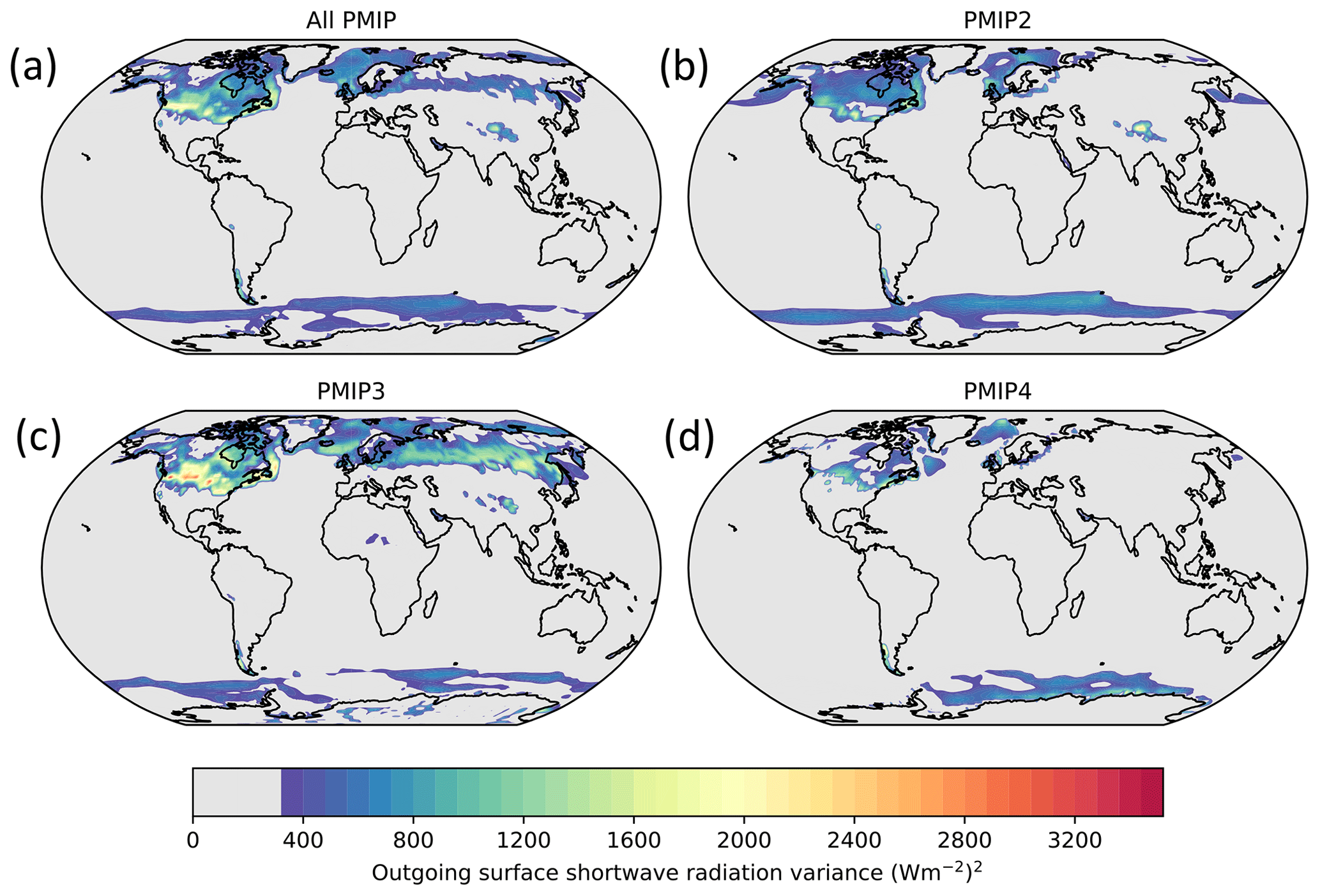
Figure 6 Maps of the variance in outgoing (reflected) surface shortwave radiation in the multi-model ensembles of (a) all PMIP generations, (b) PMIP2, (c) PMIP3, and (d) PMIP4. Variance values which are below less than 10 % of the maximum value are masked in gray, to highlight areas of high variance.

In CESM1.2 and CESM2.1, the ice sheet forcing efficacy, quantified using an adjusted forcing–feedback framework, is 1.1 and 1.9, respectively (Zhu and Poulsen, 2021; Zhu et al., 2021), which is likely connected to the cooling of Northern Hemisphere SSTs in connection with changes in wind patterns due to the topography of the ice sheets. The ice sheets, and notably the Laurentide one, are known to disturb atmospheric and ocean circulation. Notably, the Laurentide ice sheet impacts Arctic region temperature (Liakka and Löfverström, 2018), Atlantic Ocean surface winds and deepwater formation (e.g., Muglia and Schmittner, 2015; Sherriff-Tadano et al., 2018), and local cloud feedbacks (Zhu and Poulsen, 2021).

In summary, the variance in reflected shortwave radiation due to ice sheets is likely to generate noise, as the efficacy of the forcing is found to be model-dependent. Current models do not indicate whether the ice sheet forcing efficacy is above or below unity but show a substantial inter-model spread. Since the ice sheet forcing is roughly half the total forcing in LGM, this means that the ice sheet forcing, and its efficacy, could be a major source of noise in the model relationship between LGM cooling and ECS.

4.4 Surface albedo feedbacks

In response to a cooling climate, the surface albedo feedback (λ_a) is thought to strengthen as sea ice, snow cover and more reflective vegetation biomes extend. Whereas there is a broad agreement among models on this amplification, the amplitude of the state dependency in λ_a is likely model-dependent. In Table 4, we report the tropical and global λ_a after abruptly doubling CO₂ from pre-industrial and LGM conditions and abruptly halving CO₂ from pre-industrial conditions in MPI-ESM1.2-LR.

Table 4 Global and tropical (30^∘ S–30^∘ N) surface albedo feedback (λ_a) values computed with the PRP method for three simulations performed with MPI-ESM1.2-LR.

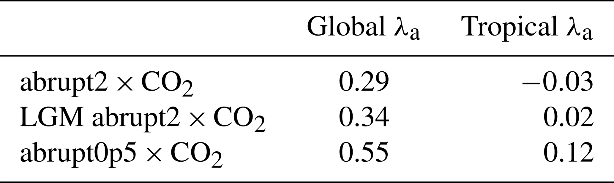
The global value of λ_a is 0.21 W m⁻² higher when halving CO₂ compared to the LGM experiment in MPI-ESM1.2-LR, which itself is only slightly higher than in the abrupt2×CO₂ experiment. In the tropical area, both abrupt2×CO₂ simulations from pre-industrial or LGM conditions show almost the same λ_a value close to zero, while the abrupt0p5×CO₂ λ_a is 0.1 W m⁻² larger. Similar findings have been made by Colman and McAvaney (2009), Yoshimori et al. (2009), and Zhu and Poulsen (2021).

The strength of the state dependency on λ_a remains difficult to estimate, but the inter-model spread in model abrupt4×CO₂ simulations is substantial, with a standard deviation of 0.09 W m⁻² K⁻¹ (Zelinka et al., 2020), which could be used as an indicator of the spread in state dependency. This magnitude would not be inconsistent with the available anecdotal single-model evidence.

In the following sections, we explore the individual contributions of snow, vegetation and sea-ice albedo feedbacks at the LGM and how their inter-model differences may act as sources of noise.

4.4.1 Snow and vegetation albedo feedbacks

Hopcroft and Valdes (2015) hypothesized that snow and vegetation albedo feedbacks might play a part in weakening the robustness of the emergent constraint by generating noise within the ensemble. In Fig. 7, we show the maps of effective surface albedo of MIROC-ESM, MRI-CGCM3, GISS-E2-R-p150 and p151, and CNRM-CM5 as well as a comparison with the PMIP3 ensemble mean. These models were characterized with unusual radiation balance changes over land compared to PMIP2 and PMIP3 models, which was suspected of generating noise in the PMIP3 emergent-constraint analysis (Hopcroft and Valdes, 2015).

Figure 7 Maps of the effective surface albedo of (b to f) several PMIP3 models and comparison with (a) the PMIP3 ensemble mean. The ensemble mean excludes the variants GISS-E2-R-p151 and MPI-ESM-P-p2, as they were excluded in the ensembles of Schmidt et al. (2014) and Renoult et al. (2020).

The model CNRM-CM5 particularly stands out as it has patches of unusually low albedo on the Laurentide, Greenland, Fennoscandian and Antarctic ice sheets. Climate models usually display different albedo for bare ice and snow, and the snow albedo is often dependent on various factors, such as snow thickness, temperature and sometimes the history of the conditions the snow has experienced. A comparison with the simulated LGM snow cover reveals that the parts of the Laurentide, Greenland, Antarctic and Fennoscandian ice sheets as well as the Andes and Himalayan mountain ranges, which show high effective surface albedo, are connected with relatively important snow cover. By contrast, the patches of low albedo are connected with less snow cover or no snow cover at all in the case of Antarctica. Central to northern Asia is also slightly covered by snow and also shows a relatively low albedo. This could indicate that the snow-free albedo of land in CNRM-CM5 is low, in particular compared to the albedo of snow-covered areas. It is not necessarily singular, as the albedo of vegetation is low and there is a large range in bare ice sheet albedo (Cuffey and Paterson, 2010), but it contrasts with the other models, where either the land ice albedo is close to the albedo of fresh snow of 0.8 or the ice sheets and forests are entirely covered by snow. Regarding the Laurentide, Antarctic and Greenland ice sheets, the areas of high snow cover are connected to lower topography, and restricted snow cover usually happens in areas of topography higher than 4000 m (Abe-Ouchi et al., 2015). Thus, it may be that topography limits more snowfall in CNRM-CM5 than in other models, which leads the average surface albedo to be dominated by the albedo of the bare ice sheet.

GISS-E2-R has a high effective albedo in northern Asia, leading to relatively cold local LGM temperatures for its low ECS. GISS-E2-R uses the prescribed LGM vegetation of Ray and Adams (2001) rather than the prescribed pre-industrial or dynamical vegetation as suggested for the PMIP3 experimental design. However, Hopcroft and Valdes (2015) noted that models with dynamical vegetation which simulated a greater loss of forest cover (e.g., MIROC-ESM) were not as cold as GISS-E2-R, implying that the vegetation map is not fully responsible for the behavior of GISS-E2-R. Instead, snow albedo and how the model handles its interaction with vegetation is likely to be responsible for this higher albedo. The representation of snow and canopy in high-latitude forests was regarded as highly challenging for general circulation models (GCMs) by the Snow Model Intercomparison Project (SnowMIP) Phase 2 (Essery et al., 2009). In the case of GISS-E2-R, the albedo of the canopy is prescribed based on vegetation type, but the reflectivity of the canopy increases when snow sticks to it (Qu and Hall, 2007; Thackeray et al., 2018). It is likely that a fraction of snow remains over the canopy in GISS-E2-R, whether it is due to too much snow, properties of the vegetation, or a fixed process simulating a high albedo for every snowfall over vegetation.

Vegetation processes and feedbacks are also important, as the implementation of dynamical vegetation has been suspected of contributing to the spread in the PMIP3 ensemble (Hopcroft and Valdes, 2015). In PMIP3, only MIROC-ESM and MPI-ESM-P-p2 included dynamical vegetation. MIROC-ESM is characterized by a substantial decrease in surface albedo in the Sahara, due to its dynamical vegetation response under LGM forcing, leading to a weak total surface albedo feedback. In Fig. 7, the comparison between MPI-ESM-P-p1 and MPI-ESM-P-p2 shows an increased effective surface albedo over Siberia compared to the static vegetation version, which is likely induced by the replacement of trees with lower-vegetation, snow-covered areas. MRI-CGCM3 is a special case as it does not have dynamical vegetation, but it exhibits a relatively strong albedo feedback, which is induced by the albedo of the areas of the LGM land mask due to the lower sea level set to the albedo of bare soil (Hopcroft and Valdes, 2015).

It is reasonable to argue that the implementation of processes such as dynamical vegetation in PMIP3 and some aspects of snow-albedo feedbacks might play a role in causing spread in the ensemble, as hypothesized by Hopcroft and Valdes (2015). However, they have a limited geographical impact and only concern a few models. Therefore, it is difficult to show that the lack of robustness of the emergent constraint would only be induced by these factors. We note that both GISS-E2-R and CNRM-CM5 have seasonal cycles of snow-albedo feedbacks matching observations of modern times (Fletcher et al., 2015; Thackeray et al., 2018), despite being locally either too cold (GISS-E2-R) or too warm (CNRM-CM5) at the LGM.

4.4.2 Sea-ice albedo feedback

Owing to the importance of sea-ice extent at the LGM, it is plausible that the LGM sea-ice albedo feedback may also contribute to a decoupling between ECS and surface temperature or SAT in those regions. In Fig. 6, we show that there is a high variance in surface shortwave radiation in polar oceans. This high variance is located towards the sea-ice edge, as there are disparities in sea-ice extent among models, with implications for the sea-ice albedo feedback. For instance in Fig. 7, the model GISS-E2-R has a small surface albedo in the Southern Ocean, indicative of a limited sea-ice extent, whereas the PMIP3 ensemble mean shows an extent equatorwards of 60^∘ S.

A spread in sea-ice albedo feedback is not necessarily an issue for emergent constraint, similarly to snow and vegetation albedo feedbacks, but it becomes a concern if models show a behavior in sea-ice albedo feedback which is not expected at first from their ECS value. This is the case for FGOALS-1.0g and ECBILTCLIO, two models with an ECS value below 2 K, which show a large extent of sea ice, where FGOALS-1.0g Arctic Ocean sea-ice extent reaches 40^∘ N at the LGM compared to 55^∘ N in the pre-industrial period (not shown). The strength of the sea-ice albedo feedback is also influenced by the presence or absence of snow, whereas the albedo of snow-free sea ice varies greatly among models. Therefore, we contend that sea-ice albedo feedback might be a contributor of noise within the ensemble of PMIP, arising from a few models. Similarly to the snow and vegetation feedbacks, the contribution is regional, and therefore the sea-ice albedo feedback is unlikely to be the main driver for the weakness of the emergent constraint.

4.5 Ocean structure and dynamics

An accurate representation of ocean circulation in models is necessary as it impacts heat transport and SST. The Atlantic meridional overturning circulation (AMOC) and the Southern Ocean dynamics are important regulators of the climate via many roles, which include energy and heat transport, deepwater formation, and interactions with sea ice. In this section we investigate the contribution of noise in the emergent-constraint framework from the AMOC and the Southern Ocean via the representation of two water masses: North Atlantic deep water (NADW) and Antarctic bottom water (AABW).

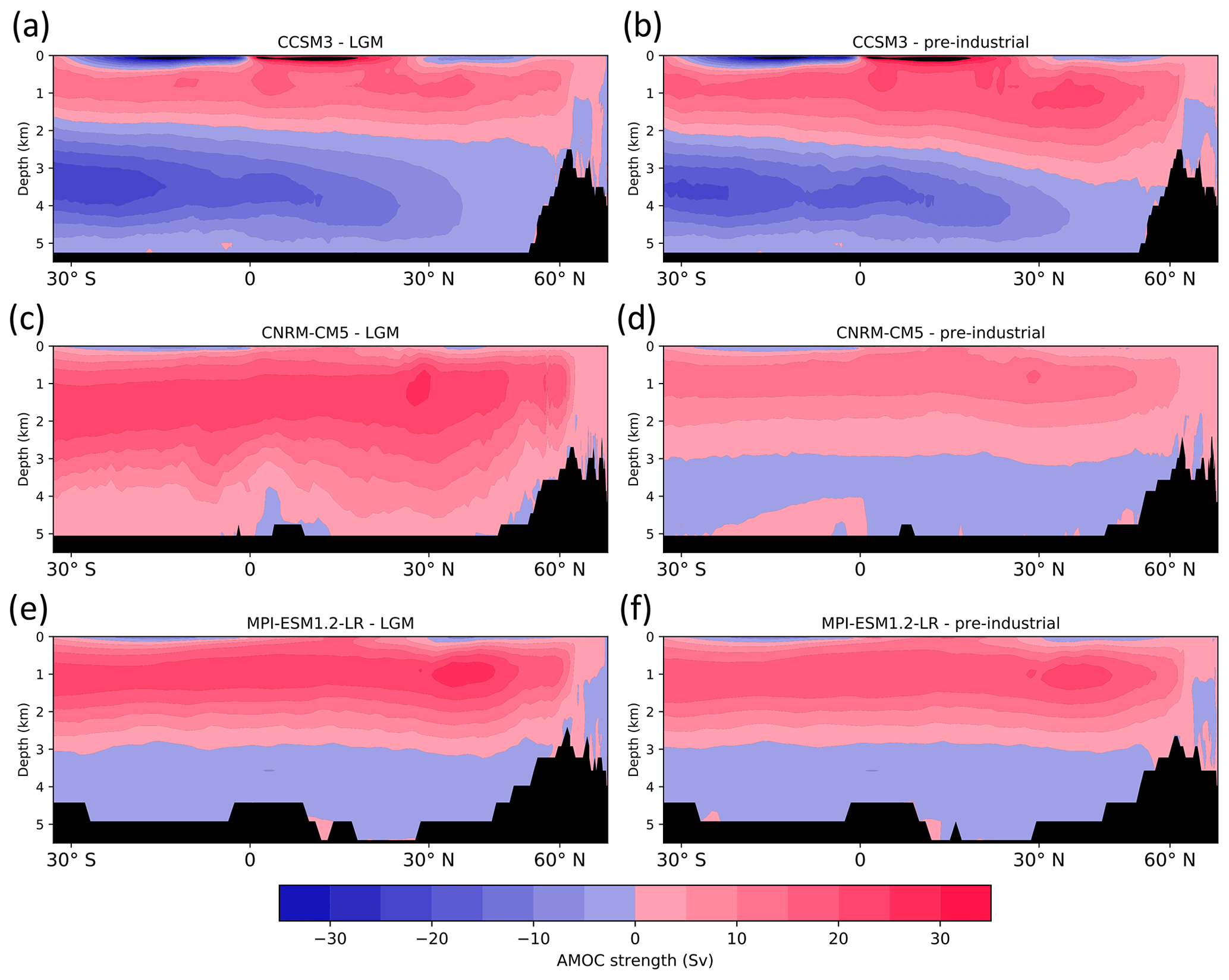
Figure 8 Examples of three typical cases of AMOC structure in PMIP models. Panels (a) and (b): AMOC in agreement with proxy data (CCSM3); (c) and (d): too deep LGM intrusion of NADW (FGOALS-g2); (e) and (f): AMOC with little difference between the LGM and the pre-industrial period (MPI-ESM1.2-LR).

4.5.1 The AMOC

Both CMIP5 and CMIP6 model ensemble means show a decline in AMOC strength in response to future warming scenarios (Weijer et al., 2020; Lee et al., 2021). This results in a Northern Hemisphere cooling as less heat is transported from the Equator to the Arctic (Jackson et al., 2015). Geological reconstructions of the LGM indicate that the glacial AMOC was as vigorous as it is in the present day (Yu et al., 1996; Lynch-Stieglitz, 2017), 30 to 40 % weaker (McManus et al., 2004) or potentially stronger (Lippold et al., 2012). Proxy data do agree that during the LGM NADW shoaled and there was a northward intrusion of AABW due to increased sea-ice extent in the Southern Ocean (Rahmstorf, 2002; Lynch-Stieglitz et al., 2007; Böhm et al., 2015; Lippold et al., 2016). Recently, Kageyama et al. (2021) showed that most of the PMIP4 LGM simulations have substantial intrusion of AABW and a shoaling of NADW for two of the models, but earlier AMOC simulations in PMIP3 and PMIP2 models were more divided (e.g., Otto-Bliesner et al., 2007; Sherriff-Tadano and Klockmann, 2021).

The representations of the AMOC can be divided into three categories, with examples provided in Fig. 8. For example, CCSM3 is one of the models which matches the proxy data fairly well, with a substantial northward intrusion of AABW and a shoaling of NADW. MPI-ESM1.2-LR is an example of a model simulating little change between the LGM and the pre-industrial period. Whereas it agrees with a proxy indicative of the strength of the AMOC being similar to the pre-industrial period, these models do not show a substantial intrusion of AABW as seen in the proxy record, and in most cases the NADW does not shoal substantially. Finally, CNRM-CM5 is an example of a model which strongly disagrees with proxy data. Here, the NADW reaches the seafloor at the LGM, and although glacial AMOC can be stronger than the pre-industrial period, proxy and 2D models do not support the LGM AMOC to be more than 10 Sv stronger than during the pre-industrial period (Lippold et al., 2012), which is the case for CNRM-CM5 and other models (Otto-Bliesner et al., 2007; Muglia and Schmittner, 2015).

It is unclear if an inaccurate representation of the AMOC has an influence on global or hemispheric temperatures and consequently on the emergent constraint between SST and ECS. Indeed, we find no relationship between by how much a model matches the proxy reconstruction of the AMOC and its Northern Hemisphere surface temperature. Models which simulate a substantial strengthening of the AMOC under the LGM forcing are not necessarily warmer, which could have been expected based on the pre-industrial simulations of Jackson et al. (2015). Moreover, the reasons behind the spread in modeled AMOC structure and strength are unclear (Sherriff-Tadano and Klockmann, 2021). Notably, the effects of density (Weber et al., 2007), salinity (Otto-Bliesner et al., 2007), wind changes driven by the Laurentide topography (e.g., Muglia and Schmittner, 2015; Sherriff-Tadano et al., 2018), or limited Antarctic sea-ice formation (Marzocchi and Jansen, 2017) have been suspected of influencing the AMOC in PMIP models.

Recently, Marzocchi and Jansen (2017) suggested that models behaving similarly to CNRM-CM5 might simulate a substantial deepening of NADW due to too short spin-up periods. In an extended 900-year-long run from its spin-up phase, the AMOC of CCSM4 shallowed by 400 m and weakened by 9 Sv, leading to values closer to proxy data (Rahmstorf, 2002; Böhm et al., 2015; Lippold et al., 2016). While the drift does not slow down after 900 years, it is not visible within the 100-year time series of PMIP3 as it is obscured by natural variability. We perform a similar analysis with MPI-ESM1.2-LR, a model which shows little change in AMOC strength and position between the LGM and the pre-industrial period. We run 621 years from the spin-up phase, which lasted 3850 years (Marie-Luise Kapsch, personal communication, 2021). The trend in AMOC strength is lower than 0.05 Sv per century compared to almost 1 Sv per century for CCSM4; thus we conclude that there is no substantial drift of AMOC in MPI-ESM1.2-LR. This could indicate that the observations of Marzocchi and Jansen (2017) are model-dependent and only affect CCSM4 or that the simulation is still not long enough or that recent PMIP4 models have an AMOC closer to equilibrium owing to their longer integration times (i.e., 6760 years for MIROC-ES2L, Ohgaito et al., 2021).

It is likely that the inter-model disagreements regarding AMOC representations contribute to the spread of models in the emergent-constraint framework. Nevertheless, we do not find a clear relationship between AMOC representations and simulated LGM temperatures, which indicates that either the different AMOC representations are compensated for on a broader scale or they are limited sources of noise for the emergent-constraint relationship.

4.5.2 Southern Ocean dynamics

Geological reconstructions strongly indicate that AABW intruded further north in the LGM owing to Southern Ocean dynamics. This intrusion is seen in very few models until PMIP4 (Kageyama et al., 2021). The models which best match proxy records show extensive annual Southern Ocean sea ice, which is known to play a part in the ocean circulation via brine rejection (Marzocchi and Jansen, 2017). Recently, Zhu and Poulsen (2021) showed that the strong coupling existing between Southern Ocean convection, upper-ocean heat convergence and sea ice contributes to a stronger LGM global cooling of ∼1 ^∘C in CESM1.2. Following that, we hypothesize that models with a large intrusion of AABW, and thus a highly convective Southern Ocean, could be relatively colder than other models with respect to their ECS. Similar to the AMOC, we do not find a clear relationship between Southern Hemisphere temperature and the representations of the Southern Ocean matching proxy data well (not shown). The spread in representations of the AABW in PMIP models is thus likely to generate noise in the emergent-constraint relationship but that noise is either small or compensated for.

We emphasize that this analysis is mainly limited to PMIP2 and PMIP3 models with limited data availability for PMIP4 models, and Southern Ocean dynamical feedbacks, which include heat transport and ocean stratification, are suspected of being model-dependent (Zhu and Poulsen, 2021). Recently, Gregory et al. (2023) found a relationship between ECS and AMOC strength in climate models in the pre-industrial period. This supports the idea that the lack of correlation between LGM AMOC and modeled temperatures is influenced by the boundary conditions of the LGM. However, improving SST biases in pre-industrial oceans at high latitudes is also shown to help LGM-modeled AMOC to match proxy data (Sherriff-Tadano and Klockmann, 2021). This might indicate either a limited noise arising from the representations of the AMOC, as biases are replicated between the pre-industrial period and LGM, or a larger noise contribution if these biases are enhanced or dampened in the cold LGM with respect to the warmer 4×CO₂ scenario from which ECS is diagnosed. Understanding the full extent of the contribution of the ocean as a source of noise would require further sensitivity experiments. Notably, variations in ice sheet topography would indicate its impact on atmosphere and ocean dynamics, or simulations with different complexity of ocean dynamics would provide information on slow ocean contributions to LGM temperatures (Zhu and Poulsen, 2021). All in all, the amplitude of the contribution of ocean dynamics in the emergent-constraint relationship is in appearance weak but is potentially underestimated, and it is likely to arise from both LGM boundary conditions and a decoupling between the cold LGM and the warm abrupt4×CO₂.

4.6 Cloud feedbacks

Cloud feedbacks (λ_cl) differ substantially across models and contribute to higher ECS in CMIP6 models (e.g., Zelinka et al., 2020). Because of different boundary conditions, λ_cl are thought to be regionally different between the LGM and pre-industrial simulations. We suspect that λ_cl are state-dependent; i.e., λ_cl calculated in a cold climate contrasts with the one computed in abrupt4×CO₂ experiments. In this section, we investigate the λ_cl between cold and warm states for a few climate models in Sect. 4.6.1 and then analyze the cloud radiative effect (CRE) of several CMIP6 models as a proxy for λ_cl in Sect. 4.6.2. Finally, we explore the effect of the mixed-phase cloud feedback on the LGM in Sect. 4.6.3, as it is challenging to represent in models and thought to be one of the main drivers behind the increase in λ_cl in CMIP6 models.

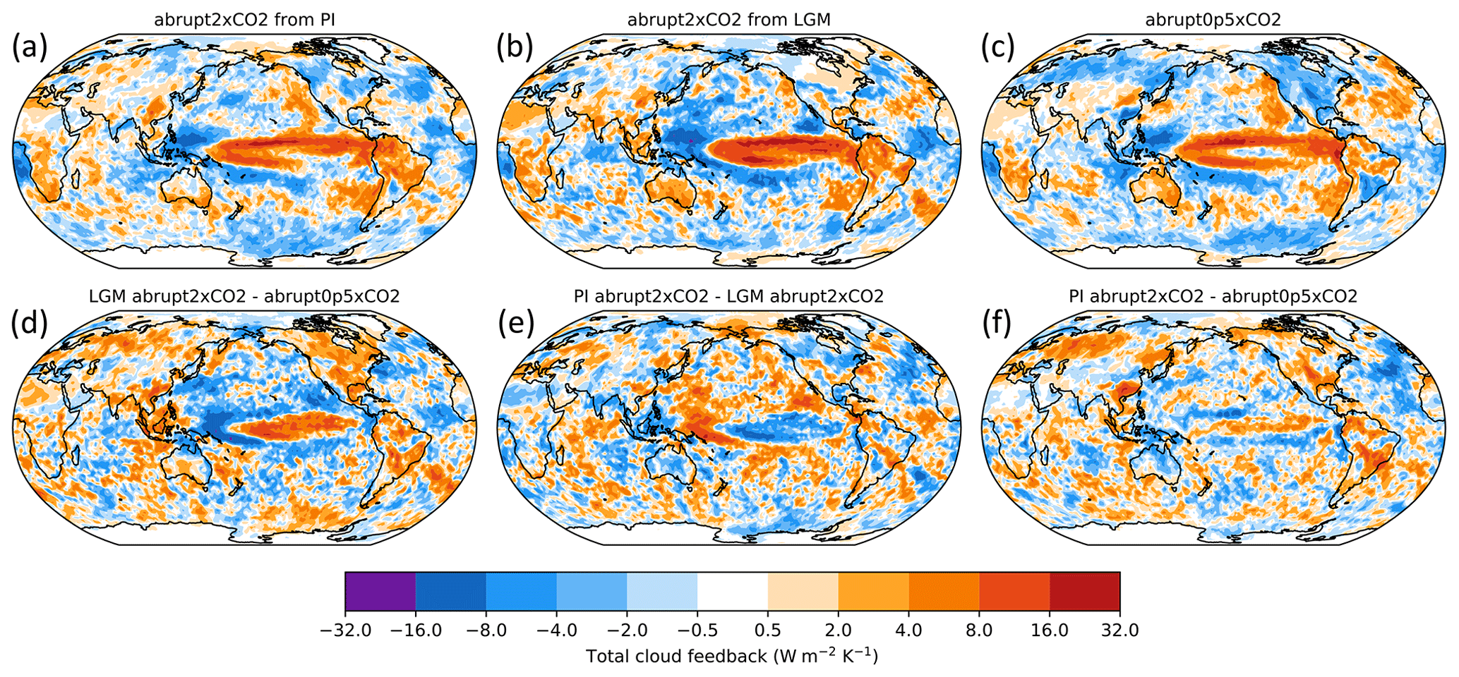
Figure 9 Cloud feedback parameters computed with the PRP method in three simulations performed with MPI-ESM1.2-LR (a–c) and differences in cloud feedbacks between the three simulations (d–f). (a) abrupt2×CO₂ from pre-industrial conditions (560 ppm), (b) abrupt2×CO₂ from LGM conditions (380 ppm), (c) abrupt0p5×CO₂ from pre-industrial conditions (180 ppm), (d) LGM-abrupt2×CO₂ minus abrupt0p5×CO₂, (e) abrupt2×CO₂ minus LGM-abrupt2×CO₂ and (f) abrupt2×CO₂ minus abrupt0p5×CO₂.

4.6.1 Single-model cloud feedbacks

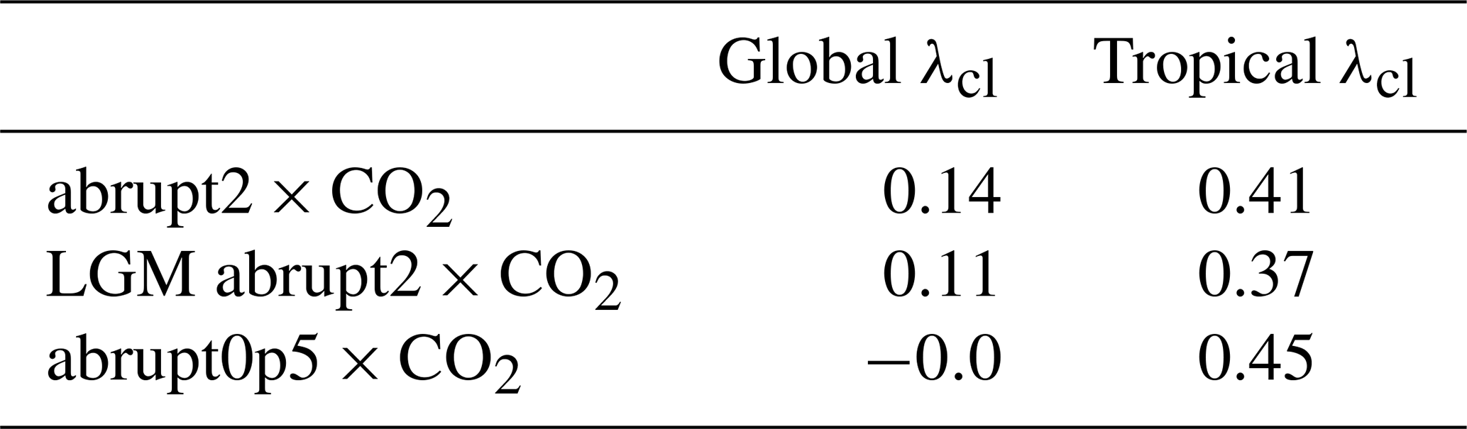
We calculate λ_cl in three sets of simulations using MPI-ESM1.2-LR to explore the state dependency between the LGM and an abrupt2×CO₂ experiment. We perform abrupt2×CO₂ from pre-industrial CO₂, abrupt2×CO₂ from LGM CO₂ and boundary conditions, and abrupt0p5×CO₂ from pre-industrial CO₂. Global maps are shown in Fig. 9, and global and tropical calculations of λ_cl are summarized in Table 5.

Table 5 Global and tropical (30^∘ S–30^∘ N) cloud feedback λ_cl values computed with the PRP method for three simulations performed with MPI-ESM1.2-LR.

In the two CO₂ doubling experiments from LGM and pre-industrial states, global λ_cl values are broadly similar and in contrast lower when CO₂ is halved. This indicates a weak global state dependency between LGM and the pre-industrial period but a more pronounced one between halving and doubling of CO₂. The LGM abrupt2×CO₂ differs notably from the pre-industrial abrupt2×CO₂ by a λ_cl near 0 W m⁻² over the Laurentide ice sheet. A near-zero λ_cl above an ice surface is physically plausible since the presence or absence of clouds cannot substantially alter the reflection to space. Changes also occur in the Pacific Ocean, where more positive λ_cl are found in the east and more negative λ_cl in the west in the LGM abrupt2×CO₂.

State dependency and forcing dependency of λ_cl have been assessed in previous studies and models. A slab ocean version of MIROC3.2 revealed substantially weaker λ_cl at the LGM than in abrupt2×CO₂ experiments (Yoshimori et al., 2009), and similar observations have been made by Zhu and Poulsen (2021) in CESM1.2. However, when comparing halving and doubling of CO₂ from pre-industrial conditions, either small differences in global λ_cl were found in the Australian BRMC model (e.g., Colman and McAvaney, 2009) or weaker λ_cl was found in the abrupt0p5×CO₂ experiment than abrupt2×CO₂ experiment in CESM1.2 (Chalmers et al., 2022).

Generalizing the results of weaker λ_cl in cold climates of CESM1.2, CESM2.1, MIROC3.2 and MPI-ESM1.2-LR is tempting, but the results from the BRMC model might indicate that the λ_cl dependency over reduced CO₂ compared to increased CO₂ could be model-dependent. Moreover, disentangling the dependency of λ_cl over the ice sheets and the greenhouse gases of the LGM is difficult, and compensations might happen at the global scale, which leads to broadly similar λ_cl between the LGM and abrupt2×CO₂ experiments. All in all, it is plausible that the influence of λ_cl on LGM temperature is model-dependent and that the decoupling between LGM λ_cl and abrupt4×CO₂ λ_cl is substantial. Since large differences are seen in the tropical Pacific in MPI-ESM1.2-LR and CESM1.2, cloud feedbacks might have been large contributors to the weakness of the tropical emergent constraint.

4.6.2 Cross-ensemble variations in CRE change

We assess how large the inter-model spread in λ_cl differences between warming and cooling could be among PMIP models based on evidence from single-model analyses. To this end, we analyze the CRE of the CMIP6 models performing abrupt0p5×CO₂ and abrupt4×CO₂ (Fig. 10). The regression of the change in CRE over surface temperature $\frac{\mathrm{\Delta }\mathrm{CRE}}{\mathrm{\Delta }\mathrm{TS}}$ is not the same as λ_cl, but variations among models in this quantity provide a good estimate of the spread of cloud feedbacks (e.g., Soden et al., 2008). If we suspect a state dependency on λ_cl, then the relationships between λ_cl and $\frac{\mathrm{\Delta }\mathrm{CRE}}{\mathrm{\Delta }\mathrm{TS}}$ should differ depending on whether $\frac{\mathrm{\Delta }\mathrm{CRE}}{\mathrm{\Delta }\mathrm{TS}}$ is computed from abrupt0p5×CO₂ or abrupt4×CO₂.

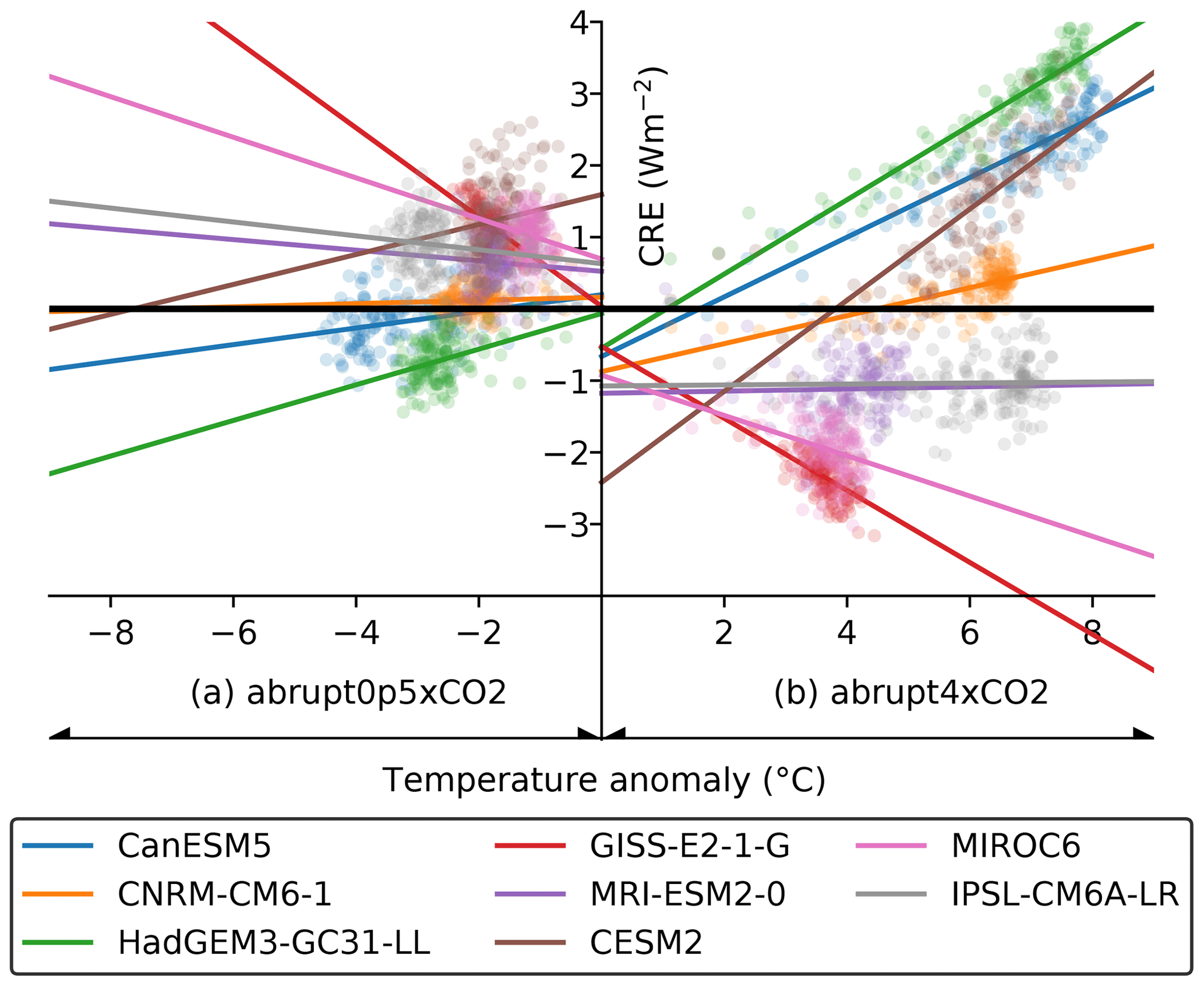
Figure 10 Cloud radiative effect (CRE) regressed on global surface temperature anomaly in abrupt0p5×CO₂ (a) and abrupt4×CO₂ (b) experiments by CMIP6 models.

For almost all models, $\frac{\mathrm{\Delta }\mathrm{CRE}}{\mathrm{\Delta }\mathrm{TS}}$ is smaller in abrupt0p5×CO₂ than in abrupt4×CO₂, which is consistent with our single-model results explored in Sect. 4.6.1. In Fig. 11, we compare the values of $\frac{\mathrm{\Delta }\mathrm{CRE}}{\mathrm{\Delta }\mathrm{TS}}$ for abrupt0p5×CO₂ and abrupt4×CO₂ with the λ_cl of Zelinka et al. (2020) calculated from abrupt4×CO₂ simulations. While the intercepts of the two regression lines are broadly similar, the slopes differ, where abrupt4×CO₂ is the steepest and abrupt0p5×CO₂ the least steep. The difference is more pronounced at higher λ_cl where the $\frac{\mathrm{\Delta }\mathrm{CRE}}{\mathrm{\Delta }\mathrm{TS}}$ differs the most. Our analysis indicates a state dependency in λ_cl in CMIP6 models, as the slope across abrupt4×CO₂ and abrupt0p5×CO₂ ensembles differs in Fig. 11. The state dependency becomes increasingly stronger with increasing λ_cl (i.e., ECS), and as the slope within the abrupt0p5×CO₂ ensemble is less steep than abrupt4×CO₂, then models can be suspected of being too warm in cooling simulation with respect to their ECS. Lastly, the dispersion of models around the regression lines indicates an inter-model spread in state dependency on λ_cl. Since λ_cl is calculated from abrupt4×CO₂, the dispersion is minimal around that line, but it is quantified as a standard error of the regression of 0.12 W m⁻² K⁻¹ for abrupt0p5×CO₂.

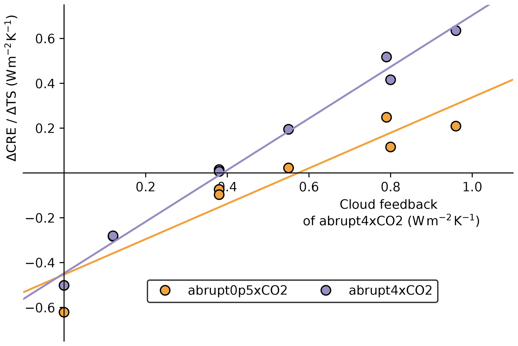
Figure 11 Comparison of the $\frac{\mathrm{\Delta }\mathrm{CRE}}{\mathrm{\Delta }\mathrm{TS}}$ slopes for abrupt0p5×CO₂ and abrupt4×CO₂ (shown in Fig. 10) with cloud feedback estimates computed from abrupt4×CO₂ in CMIP6 models (values from Zelinka et al., 2020).

We explore how a variation of 0.12 W m⁻² K⁻¹ of λ_cl impacts LGM temperatures by using a low- and high-ECS model that contributed to both LGM and abrupt0p5×CO₂ simulations. In the analysis of Zelinka et al. (2020), MIROC-ES2L and CESM2.1 have ECS of 2.66 and 5.15 K, respectively. We also use the effective radiative forcing (ERF) of 2×CO₂ and climate feedbacks as calculated in Zelinka et al. (2020). The temperature change can be computed as Eq. (4), and we estimate the LGM forcing for each model as $F_{\mathrm{LGM}}=(\mathrm{\Delta }{T}_{\mathrm{LGM}}/\mathrm{ECS})\times F_{\mathrm{2}x}$, where ΔT_LGM is −4.05 K for MIROC-ES2L (this study) and −11.3 K for CESM2.1 (Zhu et al., 2021).

$$\begin{array}{}\text{(4)}& \mathrm{\Delta }{T}_{\mathrm{LGM}}={\displaystyle \frac{-F_{\mathrm{LGM}}}{\mathit{\lambda }\pm \mathrm{0.12}}}\end{array}$$

For MIROC-ES2L, with an ECS of 2.66 K, ERF at 2×CO₂ of 4.11 W m⁻² and a total climate feedback of −1.54 W m⁻² K⁻¹, the calculated LGM temperature change is within the range −3.8 to −4.4 K. For CESM2.1, with an ECS of 5.15 K, ERF at 2×CO₂ of 3.26 W m⁻² a total climate feedback of −0.63 W m⁻² K⁻¹, the calculated LGM temperature change is within the range −9.5 to −14.0 K. Thus, CESM2.1 is more than 7 times more sensitive than MIROC-ES2L for the same forcing. This example suggests a larger impact on high-ECS models when considering the λ_cl of abrupt4×CO₂ in cooling simulations, such that at the high-end ECS, we might see more diversified LGM cooling if more models than CESM2.1 were to run the simulation. While our analyses are based on the comparison of abrupt4×CO₂ and abrupt0p5×CO₂, it is reasonable to think that the LGM could also be affected and that models underestimate the cooling. Further analyses on λ_cl at the LGM are needed, but they indicate that λ_cl could be a substantial source of noise in the emergent constraint between ECS and LGM temperature.

4.6.3 Mixed-phase clouds

The representation of mixed-phase clouds in models are important for ECS (e.g., Gregory and Morris, 1996; Tan and Storelvmo, 2016; Lohmann and Neubauer, 2018). Mixed-phase clouds are notoriously difficult to represent in numerical weather prediction and climate models (Korolev et al., 2017). However, as theory, observations and understanding of mixed-phase cloud processes have improved, their representation in models has changed substantially. Mixed-phase clouds contain a mixture of ice and liquid and exist at temperatures between 0 and −38 ^∘C. They have a strong influence on the Earth’s energy budget, and the radiative and thermodynamic properties of these clouds depend on the partitioning of cloud liquid water and cloud ice. Liquid clouds are more reflective than ice clouds and have a longer lifetime, so as the atmosphere warms and cloud ice converts to liquid, cloud albedo and lifetime increase resulting in a negative cloud-phase feedback. The cloud-phase feedback is affected by the mean state of the cloud, and cloud ice processes are important for cloud water phase in GCMs (Komurcu et al., 2014). The representation of mixed-phase clouds in GCMs has changed substantially in models in the past decade and has been identified as a plausible explanation for the large spread in ECS in CMIP6 models (Zelinka et al., 2020). In this section, we consider how these changes may have impacted the ECS and the emergent-constraint relationship in PMIP.

In PMIP2 models, the physics of mixed-phase clouds were mainly prognostic, with cloud phase dependent on a simple temperature threshold, i.e., liquid turning to ice at −15 ^∘C (Sundqvist et al., 1989). In these models the strength of the phase feedback is sensitive to the threshold temperature selected (Gregory and Morris, 1996). As liquid water path is known to exist down to −40 ^∘C, the mean-state liquid water path was usually too low and the mean state too icy. This would contribute to a strong negative cloud-phase feedback, which could lead to lower ECS estimates in these models. By CMIP5/PMIP3, the majority of models implemented ice nucleation and growth processes in their parameterizations, but cloud liquid is still underestimated at very low temperatures ($<-\mathrm{25}$ ^∘C) (Komurcu et al., 2014; Cesana et al., 2015) plausibly contributing to strong cloud-phase feedbacks and lower ECS estimates. In CMIP6/PMIP4, cloud water in the mean state increased in many models and is associated with a weakening of the cloud-phase feedback and an increase in ECS (Zelinka et al., 2020).

Some conjectures are required when considering clouds in past climates as there are no proxy records available and the variables required to analyze clouds are rarely available in the PMIP ensemble. We can speculate that in the colder LGM atmosphere, the low mean state of liquid in mixed-phase clouds in PMIP2 and PMIP3 leads to an overestimate of LGM cooling with respect to the ECS of models, whereas it is underestimated for PMIP4 models. Finally, the indirect effect of mineral dust on mixed-phase clouds has not been quantified in any generation of LGM model, although it was predicted to lead to additional cooling (Sagoo and Storelvmo, 2017). In summary it is likely that the behavior of mixed-phase clouds under LGM forcing is incomplete, and due to the lack of data, it is challenging to estimate how much noise they could contribute in emergent-constraint analysis.

4.7 Water vapor feedback

We calculate the water vapor feedback (λ_wv), which is thought to strengthen with warming (e.g., Colman and McAvaney, 2009; Mauritsen et al., 2019). In Table 6, we report tropical and global λ_wv in the abrupt2×CO₂ experiments, starting from both the LGM and the pre-industrial period and the abrupt0p5×CO₂ with MPI-ESM1.2-LR.

Table 6 Global and tropical (30°^∘ S–30^∘ N) water vapor feedback λ_wv values computed with the PRP method for three simulations performed with MPI-ESM1.2-LR.

We do not find a large difference in global and tropical λ_wv in the abrupt2×CO₂ experiments, but global λ_wv is roughly 0.2 W m⁻² lower when halving CO₂. A similar observation has been made by Colman and McAvaney (2009) with the BRMC model, but Yoshimori et al. (2009) found no change in λ_wv between an abrupt2×CO₂ and abruptly lowering to LGM greenhouse gas concentrations; Zhu and Poulsen (2021) found the same in a similar experiment. However, the full LGM simulation revealed lower λ_wv compared to a warming case (Yoshimori et al., 2009). These results indicate that state dependency in λ_wv is also model-dependent, and the inter-model spread might be of the same order of magnitude as that for λ_cl. Although there is an understanding on its increasing strength in warming climates (e.g., Colman and McAvaney, 2009; Mauritsen et al., 2019), it appears that the LGM case introduces additional complexity that may offset this general behavior. We conclude that there is a possibility of similar to stronger λ_wv in 4×CO₂ experiments compared to the LGM, which could be a source of noise in the emergent constraint.

4.8 Methane

Methane emissions from natural sources are intimately linked to global mean temperatures, with decreases in wetland methane emissions during the LGM attributed to a decrease in wetland area and lower rates of methanogenesis due to low CO₂ concentrations (Valdes et al., 2005). However, most climate models do not treat methane as a feedback but rather as a forcing since its concentration is prescribed and coupled models rarely have an active chemistry module. In abrupt4×CO₂ experiments it is usually kept fixed at the pre-industrial value, whereas in the LGM experiment it is lowered relative to pre-industrial levels. This makes methane and in general biogeochemical and biophysical feedbacks systematic biases affecting the emergent constraint between the LGM temperature and the ECS from abrupt4×CO₂.

In order to estimate the impact on the LGM emergent constraint of omitting methane feedbacks in abrupt4×CO₂ experiments, we perform a simple calculation where we calculate atmospheric methane feedback as $\mathrm{\Delta }{F}_{{\mathrm{CH}}_{\mathrm{4}}}/\mathrm{\Delta }{T}_{\mathrm{LGM}}$, where $F_{{\mathrm{CH}}_{\mathrm{4}}}$ is the forcing coming from the decrease in methane at LGM. Methane is well-constrained at the LGM (Loulergue et al., 2008) and is set at 375 ppb in the PMIP4 experiment design (Kageyama et al., 2017). Following the forcing estimates of Etminan et al. (2016), we calculate $\mathrm{\Delta }{F}_{{\mathrm{CH}}_{\mathrm{4}}}=-\mathrm{0.37}$ W m⁻² between the LGM and pre-industrial concentrations. With a global temperature change at LGM of −6.1 ^∘C (Tierney et al., 2020), the corresponding methane feedback is 0.06 W m⁻² K⁻¹.

Recent assessment of all non-CO₂ biogeochemical and biogeophysical feedbacks, in which methane feedbacks are included, have a median value of −0.01 W m⁻² (Forster et al., 2021). At the LGM, simulations using WACCM6 (Gettelman et al., 2019) show a 5 % colder LGM state than in the CESM2.1 runs, with WACCM6 having a high atmosphere model top and an active chemistry module which better capture the dynamic and chemical changes in ozone, methane and stratospheric water vapor (Zhu et al., 2022b). However, the finding differs from a previous study that suggests a 20% mitigation of the LGM global cooling by stratospheric chemistry using a different climate–chemistry model (Noda et al., 2018), implying another source of uncertainty.

4.9 Paleoclimate SST patterns and their effects

Models have roughly matched reconstructed global mean cooling in the LGM but generally have problems matching the pattern of cooling with relatively weak temperature change in the tropics and strong polar amplification (e.g., Haywood et al., 2020; Renoult et al., 2020; Kageyama et al., 2021). In parallel, focusing on the recent historical warming, attention has been paid to how patterns of the SST change can affect feedback mechanisms (e.g., Armour et al., 2013; Ceppi and Gregory, 2017). Current consensus is that the temporary pattern effect in the historical context dampens the rate of warming (Forster et al., 2021). At the same time the long-term equilibrium pattern of warming could amplify or dampen the warming (Mauritsen, 2016), but this topic is currently underexplored.

In order for an equilibrium pattern effect to alter the relationship between ECS and warming or cooling in a given paleoclimate there would have to be a difference in the boundary conditions that would alter the pattern in the paleoclimate in a way that does not happen in the idealized case of 4×CO₂. One such example could be the presence of ice sheets or differences in the ocean bathymetry or gateways. Yet, if these boundary conditions are included in the respective PMIP case and models on average respond reasonably to them, then the corresponding pattern effect is accounted for in the emergent-constraint method.

Reconstructed cooling patterns for the LGM and warming patterns in the Pliocene are, however, difficult for models to reproduce (e.g., Haywood et al., 2020; Renoult et al., 2020; Kageyama et al., 2021). Foremost, reconstructed climates exhibit a stronger polar amplified response than that simulated by most models. Presumably, such a pattern would preferentially activate the positive high-latitude feedbacks at the expense of negative tropical feedbacks, yielding a stronger global mean response which could qualify as an amplifying long-term pattern effect. Yet, the argument requires that models simulate the right long-term pattern to 4×CO₂ but not to the LGM and Pliocene boundary conditions.

It would seem that two alternative and simpler explanations are more plausible. First, reconstructions could have exaggerated polar amplifications, for instance due to using different proxies at low and high latitudes or that there are biases in the proxy calibrations that are different in warm and cold climates. Second, models may simply simulate too little polar amplification due to biases in the distribution of for instance cloud feedbacks (Burls and Fedorov, 2014). Since these biases are presumably similar in both 4×CO₂ and the Pliocene, it would not affect the emergent-constraint relationship, but it would impact the emergent-constraint relationship between 4×CO₂ and LGM where the biases differ.

5 Comparison of the sources of noise

In the previous sections, we have analyzed and reviewed sources of noise which have different geographical and physical impacts over the LGM and therefore contribute to the lack of robustness of the emergent constraint between ECS and LGM temperature. We now discuss the amplitude of each source and the nature of their contribution, which we divide into two categories:

• Structural source. The noise arises from structural uncertainties in the representation of the LGM. The source of noise has an impact on the LGM temperature but is not expected to influence the ECS of a model calculated from abrupt4×CO₂ simulation. The models might simulate lower or higher LGM temperature due to this source of noise, which will mainly modify the median inferred ECS in emergent-constraint analysis.

• State-dependent source. The noise exists because of a different behavior between the LGM and abrupt4×CO₂, such that the ECS of models might explain the LGM temperature poorly following the linear relationship given for the emergent-constraint framework. Here, we refer to a decoupling between ECS and temperature, where either non-linearity can be seen or no response at the LGM, which will mainly impact the uncertainty range on inferred ECS.

A summary of the amplitude of each source and whether it is found to be structural or state-dependent is provided in Table 7. Several sources are expected to fall into both categories; in these cases they are classified in both sources of noise.

Table 7 Assessment of the different sources of noise as well as whether they arise from structural uncertainties in representing the LGM or state dependency and varying strength between cold and warm climate. If the category of noise is written within parentheses, then it is regarded as plausible but less dominant than the category outside parentheses.

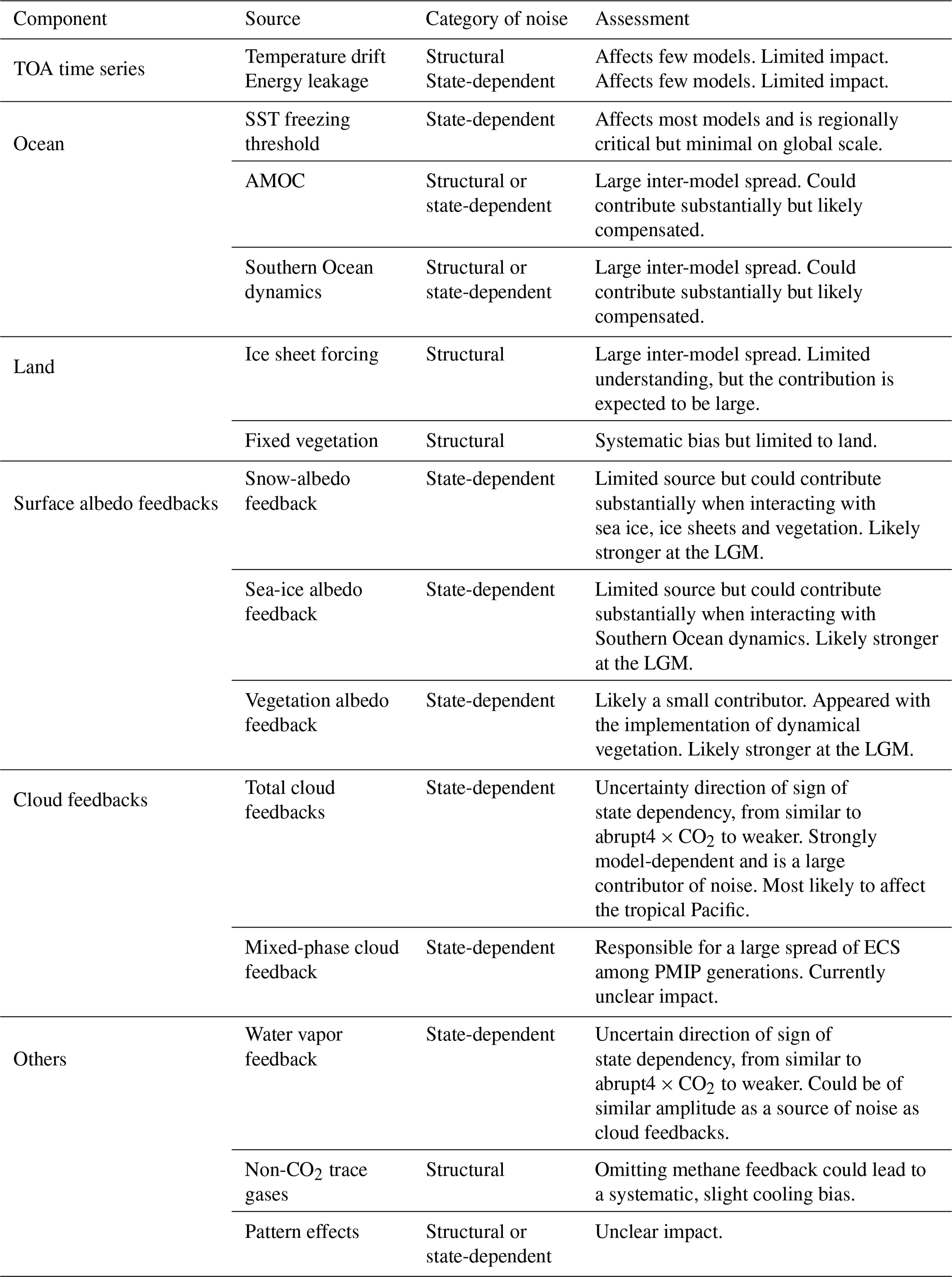
Ice sheet forcing and its efficacy is likely the main source of structural noise as it accounts for half of the radiative forcing at the LGM (Yoshimori et al., 2009; Brady et al., 2013; Kageyama et al., 2017). Ice sheet forcing is highly model-dependent, and studies indicate that the simulated temperature of the LGM might vary to a large extent across models owing to the ice sheet implementation (e.g., Shakun, 2017; Zhu and Poulsen, 2021). So far, studies quantifying this phenomenon are scarce but are valuable as other approaches to calculate ECS from LGM temperature often refer to the ice sheet forcing as an area of high albedo (e.g., Tierney et al., 2020).

The representations of both the AMOC and the Southern Ocean dynamics are likely contributors of noise, but their amplitude is less clear. Indeed, we did not find any significant relationship between AMOC and Southern Ocean convection and LGM temperature, but their impact might be compensated. The oceans also interact with the sea-ice albedo feedback, and ocean dynamical feedbacks and their connection to sea ice are found to be important at the LGM in CESM1.2 (Zhu and Poulsen, 2021). The structural issues of the AMOC and the Southern Ocean might also arises from their pre-industrial representations (Sherriff-Tadano and Klockmann, 2021), implying a state dependency in the noise. The state dependency of the AMOC has been studied for the Pliocene, where models show consistent global SST warming and strengthening of the AMOC compared to the pre-industrial period (Weiffenbach et al., 2023). Pliocene paleogeography may drive changes in AMOC rather than SSTs (Burton et al., 2022); however, the warm state of Pliocene North Atlantic SSTs enhance oceanic heat transport by the subtropical gyre, which may be responsible for regional SSTs changes (Weiffenbach et al., 2023). An additional caveat is that the simulated LGM is closer to the equilibrium response than the 150-year-long abrupt4×CO₂ simulation from which ECS is diagnosed. There are substantial differences in AMOC strength and structure between transient and equilibrated global warming experiments (Jansen et al., 2018). Generally, decadal timescale transient future simulations of the AMOC show a slowdown of the circulation (Weijer et al., 2020; Lee et al., 2021), where in turn, LGM models show slowdown, acceleration or an AMOC strength similar to pre-industrial levels, suggesting that differences and therefore noise may arise based on how close the simulation is to equilibrium. Overall, this highlights the complexity of structural issues and state dependencies in ocean currents and how they contribute as sources of noise in the emergent constraint on ECS.

The albedo of fixed vegetation, the interaction of snow on vegetation, methane feedback and the drift of model temperature due to restricted spin-up are all small sources of noise. Their impacts are limited, either acting locally (vegetation and snow) or an issue in a few models (vegetation and drift). Vegetation albedo is a structural issue, as in PMIP2 and PMIP3, most models used fixed vegetation maps, which had an impact on LGM temperature independently of their ECS, as a systematic bias. In fact, the true contribution of prescribed vegetation to the LGM cooling is difficult to constrain. It is not thought to be a dominant factor for the case of the Pliocene warming (Lunt et al., 2012), but that is based on sensitivity experiments which require interchanging ice sheets and vegetation maps between the pre-industrial period and the Pliocene. Considering the size of the LGM ice sheets, these sensitivity experiments may be biased and difficult to apply to the LGM. Nevertheless, vegetation ceases to be a structural uncertainty with the implementation of dynamical vegetation feedbacks. It seems difficult to reconcile the weakness of the emergent constraint with differences in vegetation and snow-albedo feedbacks, as hypothesized by Hopcroft and Valdes (2015). However, the additive effect of these small sources may be important in the ensemble.

The contribution of state dependency in our analysis mainly comes from climate feedbacks. Cloud feedbacks, including mixed-phase cloud feedbacks, are likely to be major drivers of noise in the emergent constraint. Cloud feedbacks, as one of the most uncertain feedbacks, are very model-dependent, with discrepancies regarding whether they are similar or weaker at LGM compared to a warming climate. They are also found to largely increase the predicted LGM temperature for higher ECS models. The inter-model spread in water vapor feedback state dependency is also an important contributor, potentially of a similar amplitude as cloud feedbacks. In theory, water vapor feedback is expected to be stronger in a warming climate than at the LGM (e.g., Colman and McAvaney, 2009; Mauritsen et al., 2019), but this is not found in all models, making its behavior complex. Finally, surface albedo feedback is a smaller source of noise among the climate feedbacks analyzed but likely plays a part in the weakness of the emergent constraint. Here, models mostly agree that surface albedo feedbacks are amplified in cooling climate, as highly reflective sea ice and snow-covered areas extend, replacing less reflective biomes such as forests. In fact, the implementation of dynamical vegetation might have amplified the inter-model spread in surface albedo state dependency but could have been compensated for by the removal of the structural uncertainties arising from prescribed LGM vegetation. As a weaker source of state-dependent noise, we include the physical bound on SST freezing which is, in fact, an issue of decoupling of temperature and abrupt4×CO₂ ECS as it mostly arises due to cold pre-industrial SST. However, it is only a regional issue and thus is a small contributor of state-dependent noise. The pattern effects are categorized as both structural and state-dependent sources of noise, but the amplitude of their contribution remains difficult to estimate and is the subject of much current research.

It is important to highlight that the definition of ECS is similar to that of the Intergovernmental Panel on Climate Change (IPCC), which includes all feedbacks except the ice sheet feedback. The latter is therefore a missing feedback in both abrupt4×CO₂, from which ECS is diagnosed, and in the LGM state. Its inclusion should therefore affect both abrupt4×CO₂ and LGM temperatures proportionately, such that climate models would be displaced along the current relationship, and therefore the regression properties should remain similar. The issues analyzed in this study are, for the most part, not missing feedbacks but arise from the lack of consistency between models. These issues are not expected to be reduced with the addition of missing feedback; on the contrary, models would have more freedom to differ from each other.

All in all, the individual inter-model spread in ice sheet forcing, cloud and water vapor feedback state dependency might be large enough to significantly change the emergent-constraint relationship. However, it is plausible that several sources are added together and some others appear as compensated, which could act further in modifying the estimates of ECS from LGM temperature.

6 Statistical view on outlier models and generational issues

A large spread in a model ensemble is advantageous to emergent-constraint methods as they are more sensitive to outliers than models near the middle of the ensemble. We explore the influence of CESM2.1, which has an ECS of 5.15 K and cools 3 K more than the next coldest model on the emergent constraint. We randomly subsample all PMIP models with a simple random sampling approach and display the distributions with and without CESM2.1 in Fig. 12. Excluding CESM2.1 does not impact the median values of slopes and intercepts, which indicates that the behavior of CESM2.1 is as expected based on the emergent-constraint relationship from other models. The correlation coefficient is, however, strongly affected by the inclusion of CESM2.1: when CESM2.1 is sampled, the correlation becomes highly significant.

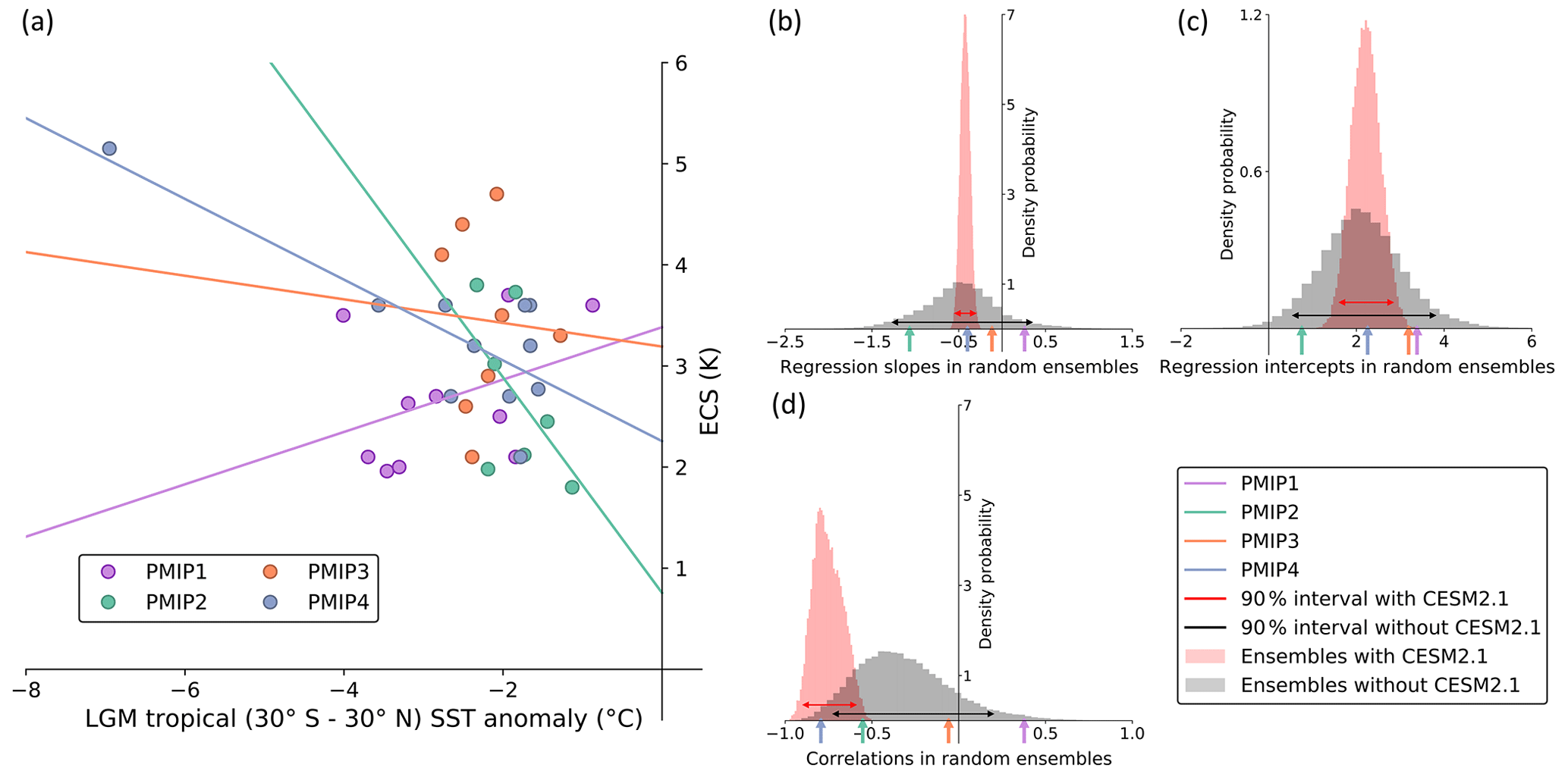
Figure 12 (a) LGM tropical SST anomaly and ECS of all models since PMIP1 and distribution of regression (b) slopes, (c) intercepts and (d) correlations from randomly sampled sub-ensemble of models. The red distribution shows ensembles where CESM2.1 was sampled, while the black distribution shows ensembles where CESM2.1 was not sampled. The colored arrows pointing at the x axis show the true values of each PMIP ensembles. Note that PMIP1 models are not available for sampling in this analysis but are only shown for comparison with other PMIPs.

The robustness of the constraint when CESM2.1 is included is encouraging. Emergent-constraint methods do not require a model to be close to the truth, but it should display a physically reasonable relationship between, in our case, the LGM temperature and ECS. In fact having a wide variety of modeled ECS, both low and high, is advantageous. The HadGEM3-GC-31-LL model, which has an ECS of 5.6 K, plans to contribute to PMIP4 (Dan Lunt, personal communication, 2021), and it will be interesting to see whether its LGM temperature is in line with its high ECS and the emergent-constraint relationship. Currently, with only one high-ECS model, the emergent-constraint analysis needs to be done with care as the high correlation might be exaggerated when including CESM2.1.

It has been suggested that inherent differences between PMIP generations contribute to the lack of correlation in the emergent constraint. Hopcroft and Valdes (2015) hypothesized that the development of new or more complex model components, for example dynamical vegetation, in PMIP3 relative to PMIP2 would generate additional noise in PMIP3 and be the cause of the lag of correlation. Thus, this might result in overconfidence in the simpler models used in the emergent constraint of Hargreaves et al. (2012). In Fig. 12, we display the true value of the investigated slope, intercept and correlation coefficient in each PMIP ensemble along with distributions from random subsamples with and without CESM2.1 described earlier in this section. Despite being relatively close to the lower end, the true value of PMIP2 is always comprised within the 5 %–95 % intervals of each parameter analyzed in randomly created sub-ensembles without CESM2.1. This indicates that the value of each parameter for PMIP2 is unlikely to arise from exceptional differences between PMIP2 and other random sub-ensembles. Therefore, the PMIP2 ensemble is not statistically discernible from the other PMIP ensembles and this does not support the hypothesis of Hopcroft and Valdes (2015).

Finally, we inspect the first-generation PMIP1 model ensemble. These models are considerably simpler and lower resolution than more recent models. These models used mixed-layer oceans with prescribed ocean heat transports rather than the three dimensional dynamic ocean models used from PMIP2 and onwards. It has been suggested that for a given model, using these mixed-layer oceans results in less cooling during the LGM than would arise if a dynamical ocean model component was used (Zhu and Poulsen, 2021). However, from a statistical point of view slope, intercept and correlation of the PMIP1 ensemble are within the ranges of randomly sampled sub-ensembles. Therefore, PMIP1 models are not statistically different from later generations with regard to the emergent-constraint analysis.

Figure 13 Comparison of the emergent-constraint relationship between global LGM surface temperature anomaly and ECS in the multi-model ensemble of PMIP4, the single-model ensemble of MPI-ESM1.2-LR (this study) and the single-model ensemble of CESM2.1 (Zhu et al., 2022a). (a) Surface temperatures are averaged over the last 50 years; (b) surface temperatures are extrapolated by linear regression until top-of-atmosphere imbalance reaches 0 W m⁻². The LGM global surface temperature reconstruction of Tierney et al. (2020) is shown as well as the LGM global surface air temperature reconstruction of Annan et al. (2022).

7 Prospects from single-model perturbed physics ensembles

Single-model perturbed physics ensembles are a convenient way of avoiding the statistical limitations which may arise from multi-model PMIP sub-ensembles, with restricted ECS and temperature ranges. In most cases, modifying cloud parameters can lead to a wide range of ECS values, but most of these ensembles are made of low-complexity models (Gregoire et al., 2011) or slab ocean models (Yoshimori et al., 2011). Slab ocean models are suspected of underestimating the LGM cooling by missing ocean dynamical feedbacks (Zhu and Poulsen, 2021) and might not be able to perfectly represent the LGM. We analyze two single-model ensembles built from coupled Earth system models (ESMs) – CESM2.1 (Zhu et al., 2022a) and MPI-ESM1.2-LR (this study) – and plot their temperature and ECS alongside the multi-model ensemble of PMIP in Fig. 13. Simulations have not been run to equilibrium in these ensembles, and the higher-ECS versions experience substantial drift of temperature. Thus, caution should be exercised when interpreting the results.

We estimate a potential equilibrium temperature by regressing the surface temperature time series with the TOA energy imbalance and show it in Fig. 13. The cooling in the higher-ECS versions is amplified, and the regression lines become almost identical to the line in the PMIP4 ensemble. This is an interesting observation, as it could suggest that inter-model structural uncertainties, which are minimal in single-model ensembles as similar versions share the same ice sheet forcing, in fact contribute little to modifying the emergent-constraint relationship. This approach is however limited, as the length of the runs is in fact too short to reach equilibrium and the control pre-industrial state also has a trend. Therefore, our temperatures obtained via regression might be greatly biased. Moreover, we filtered out three versions of CESM2.1 in this analysis, as their estimated temperatures from regression seemed unrealistically low (colder than −20 ^∘C and as low as −130 ^∘C), which made the slope of the regression line equal zero.

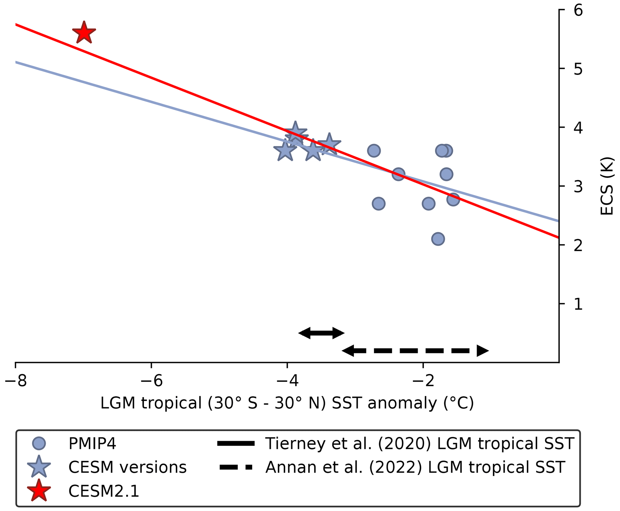
Figure 14 Emergent constraint between tropical (30^∘ S–30^∘ N) LGM SST anomaly and ECS in the PMIP4 ensemble with the addition of several CESM model family versions. The constraint is compared between the presence (red) or absence (blue) of CESM2.1. The ECS of CESM2.1 is 5.6 K, estimated from abrupt2×CO₂ in slab ocean mode (Zhu et al., 2021), for comparison with the other CESM versions. The LGM tropical SST reconstructions of Tierney et al. (2020) and Annan et al. (2022) are shown.

We create an alternate ensemble using different versions of the CESM model family that are run to equilibrium: CESM1.2, CESM1.3 and CESM2.1. The ECS range of this ensemble is narrower (3.6–4.0 K, calculated using abrupt2×CO₂ in slab ocean model configuration) and its size smaller (six models), so we expand the PMIP4 ensemble with it in Fig. 14. CESM2.1 is no longer a strong outlier, with little difference in the constraint whether CESM2.1 is included or removed. Using the tropical SST reconstruction of −3.5 ^∘C of Tierney et al. (2020), the median ECS estimate is 3.7 K with CESM2.1 and 3.6 K without. With the tropical SST reconstruction of −2.1 ^∘C of Annan et al. (2022), the median ECS is 3.1 K with and without CESM2.1. These estimates are in broad agreement with approaches based on LGM forcing estimates (e.g., Tierney et al., 2020).

Despite the progress in generating single-model ensembles, they are currently difficult to use in emergent-constraint analysis. The ensembles built from CESM2.1 and MPI-ESM1.2-LR are too far from equilibrium and would bias the estimates of ECS. Furthermore, the dependency existing between versions of the same model is also a source of concern for statistical methods, while still being poorly understood. Recent analyses show that the CESM models are substantially different from each other (Annan et al., 2022), which gives confidence in using them altogether. All in all, single-model ensembles are promising tools to study the sources of noise affecting the emergent constraint, particularly as they are expected to have reduced structural uncertainties and similar ice sheet forcing (e.g., Yoshimori et al., 2011).

8 Recommendations on paleo-emergent constraints on ECS

While the emergent constraint on ECS from LGM temperatures is weak for reasons investigated in this study, the corresponding emergent relationship from Pliocene temperatures is robust, which suggests that past climates do indeed have the potential to constrain ECS. PMIP has included several paleoclimates since its inception, with others planned for the future (e.g., Burls et al., 2021). In this section, we reflect on the issues affecting the LGM constraint and discuss what could be the ideal combinations of boundary conditions, climate states and proxy data to provide a well-constrained ECS based on past climates.

Owing to the large contribution of noise from inter-model differences in ice sheet forcing and state dependency in climate feedbacks at cold temperatures, the ideal past climate would be warmer than the pre-industrial period and with limited or no ice sheets. This is the case for the Pliocene but also for the Oligocene and Miocene and in particular for the Miocene Climatic Optimum, which is twice as warm as the mid-Pliocene warm period (Steinthorsdottir et al., 2021). Hargreaves et al. (2007) suggested a strong temperature signal for better regional correlations, as it could drastically reduce noise in polar regions. This is notably why, despite being extensively studied, the last interglacial and mid-Holocene periods are not good candidates for emergent constraints on ECS, as their temperature anomalies were small, which substantially decreases the signal-to-noise ratio. Likewise, a very warm past climate such as the Eocene is less suitable as non-linearities in feedbacks there might also appear that are not seen in abrupt4×CO₂ experiments (e.g., Caballero and Huber, 2013).

The large changes in winds, clouds, and ocean currents induced by the presence of ice sheets at the LGM suggest that important differences in climate feedbacks can arise from varying topographies. Moreover, Burton et al. (2022) showed that the closing of the Bering Strait during the Pliocene contributed to changes in North Atlantic SSTs, and Weiffenbach et al. (2023) suggests that the latter drives substantial changes in oceanic heat transport, which highlights the role of gateways in modeled global and regional paleo-temperatures. Overall, a past climate with minimal changes in non-CO₂ boundary conditions is preferable in order to reduce potentially large structural uncertainties and inter-model disagreements. In that sense, using the Miocene and older past climates is challenging, as the Pliocene was already slightly influenced by small changes in paleogeography.

Finally, the ideal past climate for constraining ECS would have abundant and high-quality proxy data. This is likely the main strength of the LGM, owing to its proximity to the pre-industrial period. Even the Pliocene, which is relatively close in time, shows large observational uncertainties that impact ECS estimates and data model comparisons, in large part because the community has decided to focus on a narrow time window (Renoult et al., 2023). Paleoclimates that are further back in time might be difficult to use in an emergent-constraint framework, as the time resolution is drastically lower, and the spatial coverage is usually poor. All in all, a synergistic combination of both the cold LGM and multiple warmer climates will, together with improved reconstructions, probably be a viable path forwards to constrain ECS.

9 Conclusions

Since its first use in an emergent-constraint framework by Crucifix (2006), the LGM temperature has often been regarded as among the best paleoclimate candidates to constrain ECS. However, the robustness of the constraint has been substantially decreasing in recent model generations, and the high end of ECS estimates from the LGM is higher than arising from the more uncertain Pliocene, which is further away in time. In this study, we have provided an assessment of the different sources of noise contributing to the weak constraint on ECS from LGM temperature.

• Sources of noise can impact the atmosphere, land and ocean either regionally or globally. Most sources have extratropical origins. Inter-model spread in ice sheet forcing and state dependency in cloud and water vapor feedbacks are regarded as the main individual contributors of noise.

• Some sources are associated with structural uncertainties in the simulation of the LGM, they are thus unlikely to affect the ECS of models computed from abrupt4×CO₂ experiments. They may bias the LGM temperature (high or low) and affect the inferred median ECS in emergent-constraint analysis. This is the case for ice sheet forcing, ocean dynamics, vegetation albedo, methane feedback and temperature drift due to limited model spin-up.

• Some sources emerge from the strength of climate components varying between cold and warm climate. These are linked to state dependency and lead to a decoupling of the ECS of abrupt4×CO₂ and LGM temperature. These sources are likely to affect the uncertainty range of inferred ECS, as they disrupt the linear relationship given in the emergent-constraint framework. This is the case for cloud, water vapor and surface albedo feedbacks as well as the physical bound on SST cooling temperature and SST pattern effects.

• There is no significant difference between the temperatures of PMIP2, PMIP3 and PMIP4. Whereas some sources of noise might be larger in individual PMIPs, such as the state dependency in surface albedo feedback arising from the implementation of dynamical vegetation, this does not seem to lead to statistically different PMIP ensembles.

• The constraint is critically affected by outlier models, i.e., high- and low-ECS models. Currently, there is only one high-ECS model (CESM2.1, ECS = 5.15 K) which is responsible for the apparent high correlation between LGM temperature and ECS. The inclusion of further high-ECS models, such as HadGEM3-GC31-LL, would provide additional information on the high end of the ensemble.

While there are several large sources of noise, the additive impact of smaller sources may be equally important. The quantification of sources remains difficult as it would require sensitivity experiments which do not necessarily exist, and it is likely that compensation processes are at work. Furthermore, the most uncertain sources, such as mixed-phase cloud feedbacks and SST pattern effects, might have been overlooked and could be responsible for a larger noise.

The LGM is currently a weak emergent constraint on ECS but is broadly consistent with inferences from data-assimilation and forcing estimate methods (e.g., PALAEOSENS Project Members, 2012; Sherwood et al., 2020; Tierney et al., 2020) but gives a wider range of uncertainty. This could indicate that either emergent-constraint approaches are considering too many sources of noise or that forcing-based methods lead to narrow results.

In comparison, the Pliocene is a robust constraint in both emergent-constraint and forcing-based methods (Hargreaves and Annan, 2016; Sherwood et al., 2020; Renoult et al., 2020). This might be due to the state dependency effect between abrupt4×CO₂ and the warm Pliocene being more limited than with the LGM temperature. However, several factors might be neglected for the case of the Pliocene, notably in structural uncertainties.

The LGM is still the most expanded paleo-ensemble of simulations and therefore remains of particular interest for emergent-constraint purposes. Sets of sensitivity experiments involving ice sheet topography, vegetation maps or sea ice and ocean dynamics would provide useful information on the reasons of noise as well as the contributions from high-ECS models, both of which already benefit the Pliocene. This could give a better understanding of poorly understood phenomena, such as a state-dependent climate feedbacks and ice sheet forcing efficacy, and increase the robustness of the emergent constraint on ECS from LGM temperature.