the Creative Commons Attribution 4.0 License.
the Creative Commons Attribution 4.0 License.
 | 14 Dec 2023
Hysteresis and orbital pacing of the early Cenozoic Antarctic ice sheet
Jonas Van Breedam
Philippe Huybrechts
Michel Crucifix
The hysteresis behaviour of ice sheets arises because of the different thresholds for growth and decline of a continental-scale ice sheet depending on the initial conditions. In this study, the hysteresis effect of the early Cenozoic Antarctic ice sheet to different bedrock elevations is investigated with an improved ice sheet–climate coupling method that accurately captures the ice–albedo feedback. It is shown that the hysteresis effect of the early Cenozoic Antarctic ice sheet is ∼180 ppmv or between 3.5 and 5 ∘C, depending only weakly on the bedrock elevation dataset. Excluding isostatic adjustment decreases the hysteresis effect significantly towards ∼40 ppmv because the transition to a glacial state can occur at a warmer level. The rapid transition from a glacial to a deglacial state and oppositely from deglacial to glacial conditions is strongly enhanced by the ice–albedo feedback, in combination with the elevation–surface mass balance feedback. Variations in the orbital parameters show that extreme values of the orbital parameters are able to exceed the threshold in summer insolation to induce a (de)glaciation. It appears that the long-term eccentricity cycle has a large influence on the ice sheet growth and decline and is able to pace the ice sheet evolution for constant CO2 concentration close to the glaciation threshold.
- Article
(14944 KB) - Full-text XML
-
Supplement
(8162 KB) - BibTeX
- EndNote


The concern about nonlinear dynamics in the climate system has recently increased given the possible collapse of the West Antarctic ice sheet (Rosier et al., 2021) and the Greenland ice sheet (Boers and Rypdal, 2021). These so-called tipping points are thresholds beyond which self-reinforcing feedbacks could irreversibly lead to a new state (Lenton et al., 2019; Armstrong McKay et al., 2022). These thresholds might trigger other tipping points and could result in a tipping cascade (Klose et al., 2020). For instance, melting of the Greenland ice sheet could halve the strength of the thermohaline circulation in the North Atlantic when large amounts of meltwater are released from the ice sheet (Van Breedam et al., 2020; Li et al., 2023).
The build-up of the Antarctic ice sheet around the Eocene–Oligocene transition (EOT) is also a tipping point and occurred at a time that environmental conditions were satisfactory for ice sheet growth, ensuring a series of positive feedbacks, eventually leading to the formation of a large ice sheet. These environmental conditions included the thermal insulation of Antarctica by ocean currents (Kennett, 1977), wind patterns (Houben et al., 2019) or both; the decline in carbon dioxide concentrations (Pagani et al., 2011); and tectonic activity that moved the Antarctic continent closer to the South Pole. Geological evidence (Scher et al., 2014; Carter et al., 2017) and modelling work (Van Breedam et al., 2022) also pointed to ephemeral glaciations prior to the EOT. This would imply that thresholds in the climate system were first crossed to initiate and end large-scale glaciations during the late Eocene.
Once environmental conditions are sufficient for ice sheet growth, a small change in climate conditions can trigger a large, nonlinear response. It is generally believed that orbital parameter variations are the cause of large ice sheet changes and have regulated ice sheet growth and decline during almost any geological period in the history of the Earth (Mitchell et al., 2021). These interpretations arise from the identification of periodic events observed in geological archives and are attributed to reflect Milankovitch cycles (De Vleeschouwer et al., 2017). The main influence of changes in the orbital parameters on the climate system is a seasonal and latitudinal redistribution of incoming solar radiation. The different orbital parameters each have a different periodicity. The precession has periods of 19 and 23 kyr, the obliquity of 41 kyr, and the eccentricity around 100 and 405 kyr (Laskar et al., 2011). Especially the eccentricity has been thought to play a crucial role in the ice sheet stability (Horton et al., 2012).
Hysteresis is the dependence of a physical system based on its history. The ice sheet–climate system exhibits hysteresis where, for a given forcing, either a large ice sheet or a small ice sheet and bare bedrock are stable states. Which one is reached depends on the initial conditions. For instance, when CO2 concentrations are very low, a large continental ice sheet can exist and it will be far from a tipping point (Fig. 1). As CO2 concentrations (control parameter) increase, the system gets closer to a tipping point and will eventually make an abrupt change towards a new system state without the ice sheet. The underlying mechanisms to induce the nonlinear changes are the ice–albedo feedback and the elevation–surface mass balance feedback.
In previous work, the hysteresis behaviour of ice sheets has been investigated to determine the future thresholds for ice sheet stability of the Greenland ice sheet (Letréguilly et al., 1991; Ridley et al., 2005, 2010; Robinson et al., 2012; Levermann and Winkelmann, 2016) and the Antarctic ice sheet (Huybrechts, 1994; Garbe et al., 2020). Hysteresis of ice sheet volume variations has been identified during the Quaternary ice ages to explain the 100 kyr cyclicity of prolonged ice sheet build-up and rapid deglaciation (Calov and Ganopolski, 2005; Abe-Ouchi et al., 2013).
Pollard and Deconto (2005) determined the hysteresis of the early Antarctic ice sheet at the Eocene–Oligocene transition using an isostatically rebounded present-day bedrock topography and a matrix method where a limited number of climate model runs were performed based on end members in the forcing. The adopted approach captured the important height–mass balance feedback. However, the ice–albedo feedback may not have been properly taken into account, given the small set of initial ice sheet geometries used in that study. Furthermore, beyond the positive height–mass balance and ice–albedo feedbacks, a negative feedback from isostasy might arise during the build-up and decline of a continental-scale ice sheet (Crucifix et al., 2001). The solid Earth will deform in response to ice mass loading, and as a result, the surface elevation increase due to increased accumulation of ice will be delayed. It is proposed that this negative feedback will also delay grounding line migration in the marine sectors of Antarctica during the coming centuries (Larour et al., 2019).
In this study, the hysteresis of the early Cenozoic Antarctic ice sheets is tested with an improved methodology based on an emulator calibrated on 20 predefined ice sheet geometries. This number of different ice sheet geometries allows the climate model to represent the climatic state for a small change in the surface type, being either ice or tundra. This way, the albedo effect from a change in ice sheet area is well-captured. The sensitivity of the threshold behaviour to different recent palaeo-bedrock elevation reconstructions is tested. Since isostasy has a potentially significant impact on the glaciation threshold, sensitivity tests are performed to assess the strength of the isostatic adjustment feedback on the ice sheet growth. Additionally, the importance of the orbital parameters for the glaciation and deglaciation thresholds is investigated. Constant forcing simulations are run to explore the influence of the eccentricity, the obliquity, and the CO2 values on glaciation and deglaciation thresholds. At the same time, this study also aims at identifying the forcing needed to initiate and end a continental-scale glaciation when the Earth again entered icehouse conditions in the early Cenozoic.
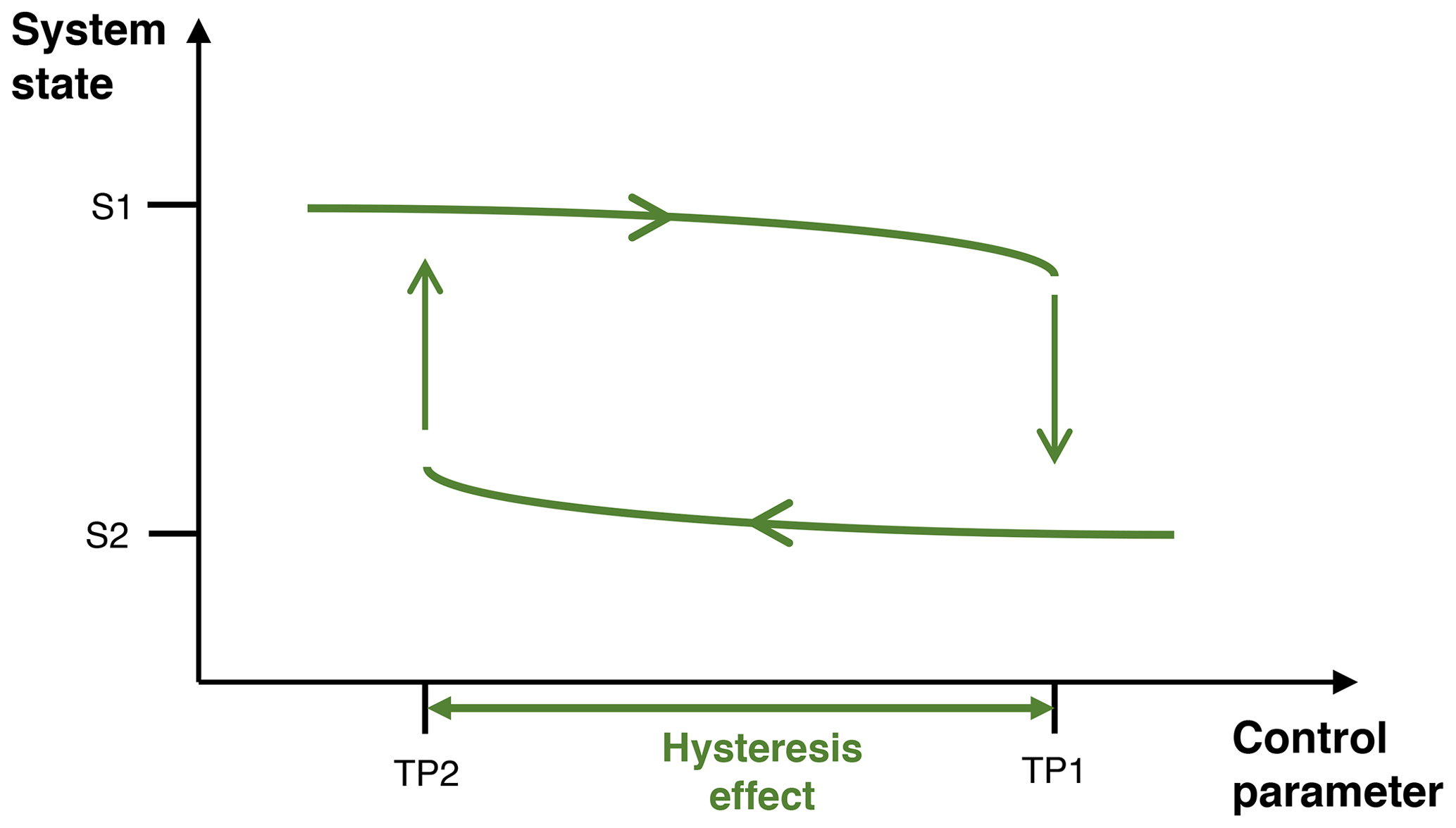
Figure 1Typical diagram visualizing the concept of the hysteresis effect. The system state is either a continental-scale ice sheet (S1) or no ice sheet (S2). The control parameter can be the surface temperature or the forcing itself such as the CO2 forcing or the insolation forcing. TP1 and TP2 represent tipping points at which the system can quickly change its state.
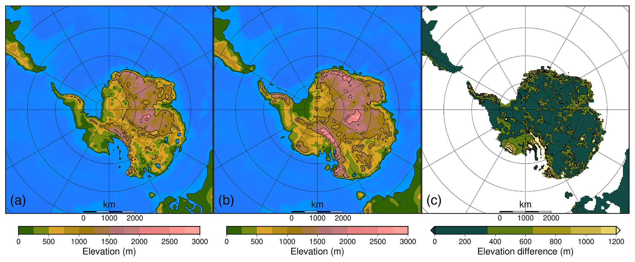
Figure 2(a) Minimum and (b) maximum bedrock elevation reconstructions from Wilson et al. (2012). (c) The elevation difference between the maximum and minimum bedrock reconstructions.
The different models used in this study are the climate model HadSM3 and the ice sheet model AISMPALEO. The models interact with one another through the Gaussian process emulator CLISEMv1.0 (Van Breedam et al., 2021b).
2.1 Climate model HadSM3
The coupled atmosphere–slab ocean climate model HadSM3 (Williams et al., 2001) provides the climatic fields. The resolution of the atmospheric component is 2.5∘ for the latitude and 3.75∘ for the longitude. It has a hybrid vertical coordinate with 19 levels in the vertical (Pope et al., 2000). The heat fluxes between the surface and the atmosphere are calculated with the MOSES-1 scheme (Cox et al., 1999). The slab ocean model equilibrates with the atmosphere in a 50 m thick layer where heat is exchanged with the atmosphere. In slab ocean–atmosphere models, an anomalous heat convergence is added to the ocean to mimic the real influence of oceanic circulation below the slab layer. Monthly variable zonal mean sea surface temperatures (SSTs), representative for the late Eocene (Evans et al., 2018), are prescribed to calibrate the anomalous heat convergence. These heat fluxes, representative for the horizontal heat transport and seasonal deep-water exchange, are then used to simulate realistic sea surface temperatures under various climate conditions. Sea ice is simulated during the winter months and is mostly constrained to the Weddell Sea region, but it disappears again during the austral summer in most simulations. The palaeogeographic reconstruction is based on the method presented in Baatsen et al. (2016) using the van Hinsbergen et al. (2015) plate rotational model. The bedrock topography used in the climate model is the Wilson maximum bedrock topography (Wilson et al., 2012) and is representative for the Eocene–Oligocene transition (EOT) at 34 Ma (Fig. 2). The minimum and maximum bedrock topographies are applied as a boundary condition in the ice sheet model at a 40 km resolution. In order to grasp the entire uncertainty, each ice sheet model grid cell takes on the lowest and highest value for the minimum and maximum bedrock topography, respectively, from the original higher-resolution Wilson et al. (2012) dataset within each ice sheet grid cell.
2.2 Emulator CLISEMv1.0
The emulator CLISEMv1.0 (Van Breedam et al., 2021b) is used to force the ice sheet model during the multi-million-year simulations. The emulator is calibrated on 100 preliminary climate model runs from HadSM3, which is forced with a unique combination of the orbital parameter ε (obliquity) and the parameter combinations esin ϖ and ecos ϖ, where e is the eccentricity and ϖ is the longitude of the perihelion. The 100 climate model runs also sample 20 different ice sheet geometries, ranging from a very small ice cap in the Gamburtsev Mountains up to a fully glaciated Antarctic ice sheet. The geometries have been chosen such that their ice volumes have a good spread between the smallest and the largest ice sheet geometries. The use of 20 different ice sheet geometries is equivalent to grasping the surface type differences at the resolution of the climate model, and therefore the albedo changes can be fully captured. The albedo varies between the discrete values of 0.8 for ice–snow and 0.2 for tundra. The CO2 forcing across the runs ranges from 550 to 1150 ppmv. After a calibration and validation process of the 100 preliminary climate model runs (see for details Van Breedam et al., 2021a), the emulator is able to provide the climatic forcing (temperature and precipitation fields) necessary to drive the mass balance of AISMPALEO for any combination of the orbital parameters, the CO2 level and the ice sheet volume (Eq. 1). The orbital parameter combinations (Laskar et al., 2011) and the CO2 concentration are prescribed, while the ice sheet volume (Vice) is calculated within the ice sheet model. The emulator set-up is the same as EMULATOR_20 calibrated on ice volume as presented in Van Breedam et al. (2021a), which has been applied to the late Eocene to investigate the potential for late Eocene glaciations (Van Breedam et al., 2022). The climatic fields are updated every 500 years in the ice sheet model, a time step that is sufficient to capture the feedbacks between the ice sheet and the external forcing (Herrington and Poulsen, 2011).
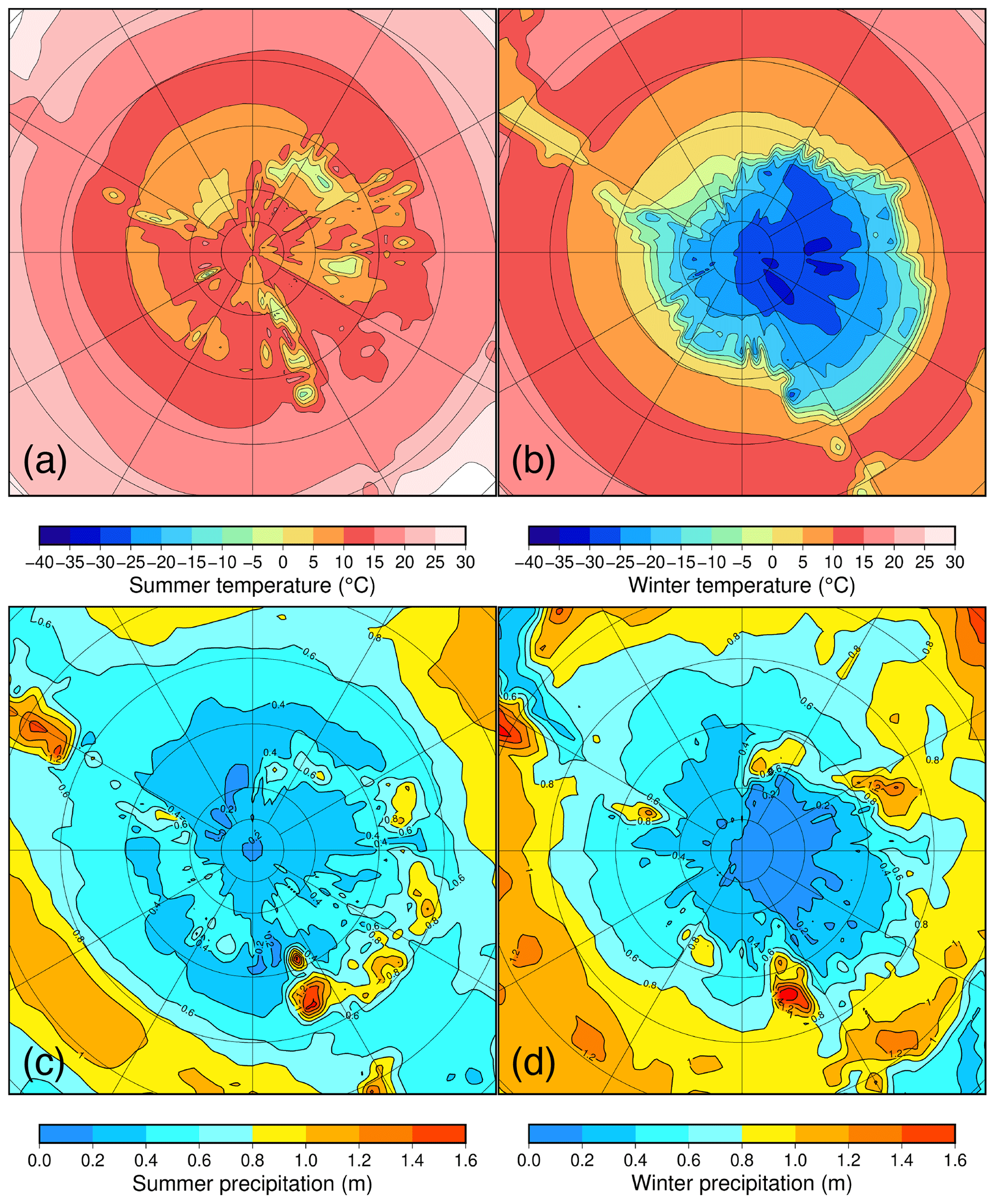
Figure 3Antarctic climatologies for a 2× pre-industrial CO2 forcing (560 ppmv). (a) Summer (DJF) temperature. (b) Winter (JJA) temperature. (c) Summer (DJF) precipitation. (d) Winter (JJA) precipitation.
The simulated Antarctic climate is strongly dependent on the forcing. In Fig. 3, seasonal temperature and precipitation patterns are shown for a nearly ice-free Antarctica with a few small ice caps at the highest elevations only. Here, the CO2 forcing is representative of a 2× pre-industrial CO2 forcing (560 ppmv), the obliquity is close to the present-day obliquity with 23.4∘ and the eccentricity is very small (0.007), resulting in an almost circular orbit; therefore, the effect of the precession is negligible. The precipitation is largest along the Antarctic continental margin and decreases inland. There is a lower precipitation rate during the austral winter (June–July–August or JJA) than during the austral summer (December–January–February or DJF) above the Antarctic continent. In winter, most precipitation falls as snow, while snowfall is limited to the highest-elevation regions such as the Gamburtsev Mountains and Dronning Maud Land in summer. The seasonality is extremely large on the Antarctic continent with a winter–summer difference in mean daily temperatures of 30–35 ∘C along the continental margin up to 50–55 ∘C in the interior of the continent close to the South Pole. This is in line with the study from Baatsen et al. (2020) using CESM 1.0.5, who identified a large seasonality of 35–45 ∘C on the Antarctic continent and a monsoonal type of climate with larger summer precipitation.
2.3 Antarctic ice sheet model AISMPALEO
The three-dimensional thermomechanical ice sheet model AISMPALEO is used at a resolution of 40 km. The model has 30 levels in the vertical, with a closer spacing towards the bedrock where most of the shearing occurs. Grounded ice flow is calculated using the shallow ice approximation (SIA), while ice shelf flow is derived from the shallow shelf approximation (SSA) in case the ice sheet reaches the ocean. Grounded ice flow is a result of internal deformation and basal sliding at locations where the pressure melting point is reached (Huybrechts and de Wolde, 1999). The basal sliding velocity in AISMPALEO follows a Weertman relation and is proportional to the third power of the basal shear stress and inversely proportional to the height above buoyancy. The basal sliding coefficient is a constant multiplication factor for the basal sliding and equals N−3 yr−1 m8. The sensitivity of the ice sheet model to ice sheet parameter uncertainties is not explored. An enhancement factor of 1.8 is used for grounded ice. This is similar to the value used to model the present-day Antarctic ice sheet with AISMPALEO. A constant geothermal heat flux of 50 mW m−2 has been applied over the entire model domain.
The grounding line is a transition zone one grid cell wide between the grounded and floating ice where all the stress components contribute in the effective stress in the flow law. Ice shelves develop when the grounded ice reaches the coast and the influx of snow from the atmosphere and ice from upstream exceeds the sum of surface ablation and basal melting. Although the slab ocean model exchanges heat with the atmosphere and records changes in the sea surface temperature, we do not use this information to calculate basal melt rates. Instead, we prescribe a constant basal melt rate of 10 m yr−1 over the entire domain. This is a strong simplification (and perhaps it is even too low in some locations). It allows small ice shelves to develop once the ice sheet reaches the coast. Nevertheless, even for present-day simulations large uncertainties exist in how changes in ocean temperature and salinity affect melt rates below the ice shelves (Burgard et al., 2022). There is no special treatment of calving fronts, and iceberg calving occurs when the ice shelf front is thinner than 150 m.
The surface mass balance is computed using the efficient positive degree day (PDD) model (Janssens and Huybrechts, 2000). The PDD model uses the yearly sum of the mean daily temperatures above 0 ∘C to determine the melt potential. In practice monthly time steps are sufficient to calculate the total number of PDDs. Random weather fluctuations and the daily cycle in temperature are taken into account by including a standard deviation of the mean daily temperature of 4.2 ∘C. Different degree day factors (DDFs) are used to melt snow and ice: 0.003 m ice equivalent ∘C−1 d−1 and 0.008 m ice equivalent ∘C−1 d−1, respectively. The melt rate is computed by multiplying the DDFs of snow and ice by the sum of the PDDs. The difference between snow and rain is calculated based on a surface temperature threshold of 1 ∘C. When ice is melting, some of the meltwater can be retained or refreeze in the snowpack to form superimposed ice.
The model includes a component to calculate isostatic adjustment due to ice mass addition and removal. The isostatic model consists of an elastic lithosphere with a flexural rigidity D of 1025 Nm (which is a measure of the strength of the lithosphere) on top of a viscous asthenosphere to allow the crust to deform far beyond the local ice loading (Huybrechts, 2002). The vertical deflection of the lithosphere w is given by a fourth-order differential equation (Eq. 2) Here, q is the ice load, ρm the mantle density (3300 kg m−3) and g the gravitational acceleration. This equation is solved using a Kelvin function of zero order (kei). The viscous asthenosphere responds to the ice load with a relaxation time τ of 3000 years (Le Meur and Huybrechts, 1996).
2.4 Experimental design
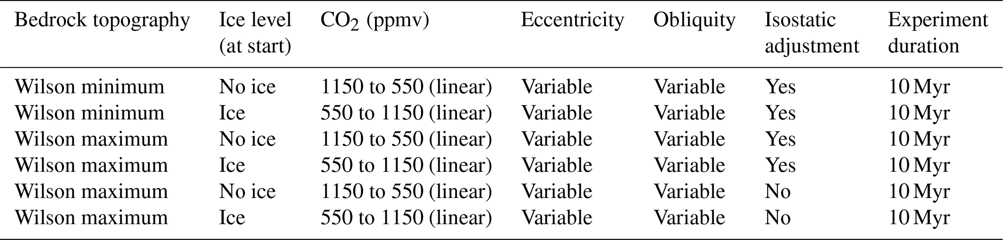
All simulations span the time period between 40 and 30 Ma, for which the orbital forcing for the different simulations is provided. Because the initial bedrock topography has a large influence on the ice sheet inception and also on the size of the continental-scale ice sheet, simulations are performed for the minimum and maximum bedrock topography estimates from Wilson et al. (2012) in order to test the hysteresis and threshold behaviour for two extremes (Figs. 2 and S1). Sea level changes (sea level fall when the ice sheet is growing) are not included as an additional forcing because the number of grid points that would become land-based if sea level fell by −70 m is very limited. The simulations that start from a bare bedrock are forced with an atmospheric CO2 concentration linearly decreasing from 1150 to 550 ppmv. The resulting continental-scale ice sheet extent is then used for the simulations starting from a glaciated continent, and the CO2 concentration is linearly increased from 550 to 1150 ppmv (Table 1). The lower and upper bounds of the CO2 concentration are chosen to include a forcing when either the ice sheet grows to a continental scale for any astronomical forcing (550 ppmv) and a forcing that is too high to allow any ice sheet to exist (1150 ppmv) in our model set-up. Additional sensitivity experiments are performed in which isostatic adjustment is not considered.
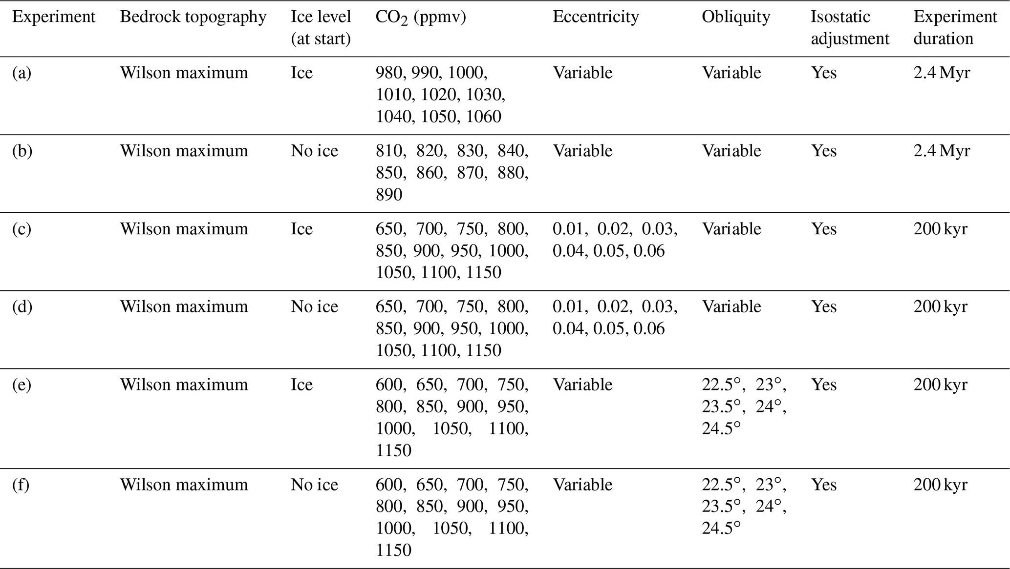
Table 1Standard set of experiments with the Wilson minimum and Wilson maximum bedrock topography as boundary conditions and variable orbital forcing.
An additional set of runs (Table 2) explores the variation in orbital forcings to investigate the influence of the insolation thresholds for ice sheet growth and decline in detail. In these runs, different values for the individual orbital parameters or the insolation are the control parameters explored (see Fig. 1 and Table 2), and the CO2 concentrations are kept constant. The orbital parameter solution La2010 from Laskar et al. (2011) is used (Fig. 4). The orbital parameters contain periods ranging from about 20 kyr for the precession up to 405 kyr for the long-term cycle in the eccentricity. On a multi-million-year timescale, the eccentricity also exhibits variations with a longer period. Spectral analyses reveal that this cycle has a main periodicity of 2.4 Myr (Laskar et al., 2004). The duration of the experiments wherein the influence of the eccentricity is investigated is 2.4 Myr long starting at 34.2 Ma up to 31.8 Ma to capture the extrema when the 100 kyr, 405 kyr and 2.4 Myr cycles reach a maximum, separately and combined. In the latter experiments, the CO2 forcing is explored in a narrow window of 80 ppmv at an interval of 10 ppmv. The other experiments wherein the eccentricity is constant and the obliquity is variable or the obliquity is constant and the eccentricity is variable are sampled in a larger CO2 window of 450 ppmv at an interval of 50 ppmv (Table 2). These experiments have a duration of 200 kyr because they equilibrate faster with the forcing (there is a limited influence of changes in the orbital forcing).
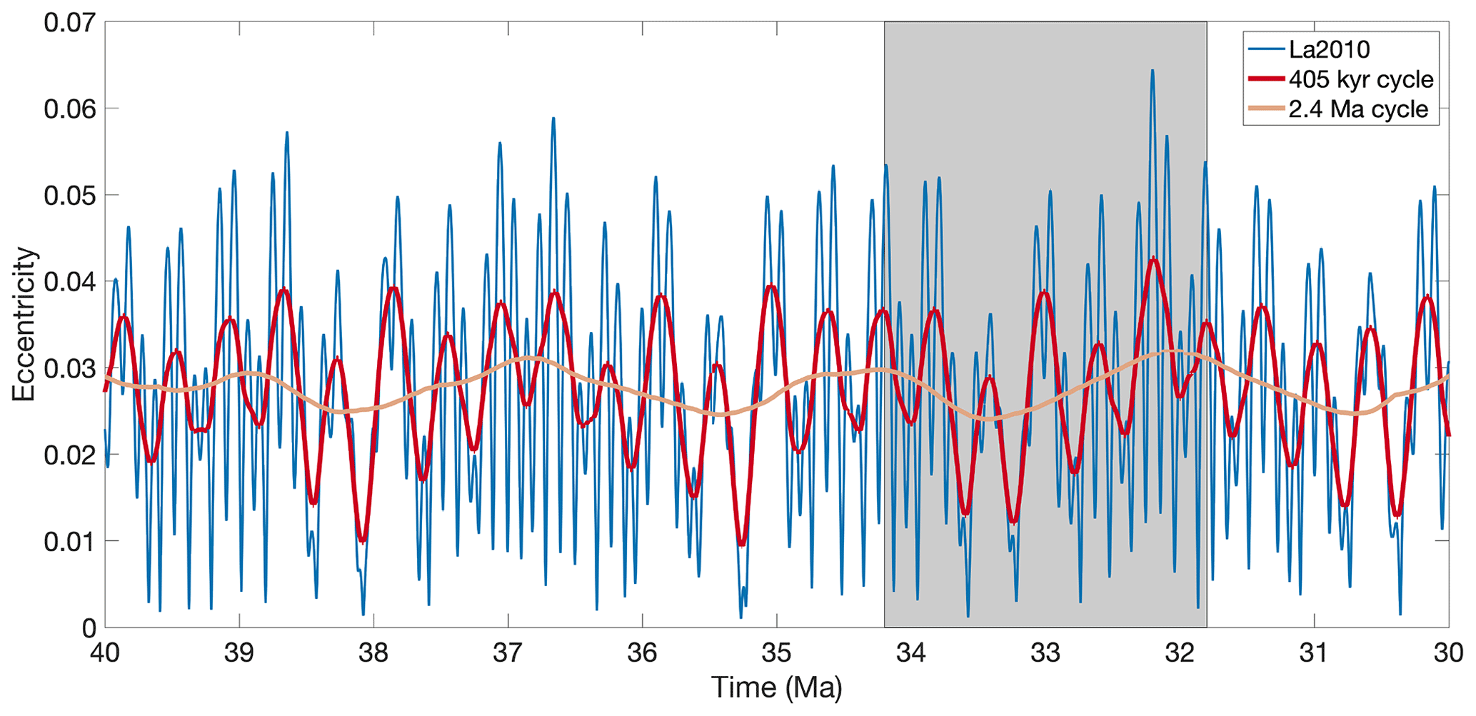
Figure 4Earth's orbital eccentricity between 40 and 30 Ma using the La2010 orbital solution (Laskar et al., 2011). The ∼100 kyr cycle (blue) is clearly visible. The 405 kyr cycle (red) and 2.4 Myr cycle are visualized by applying a running mean to the eccentricity from the La2010 solution. The period between 34.2 and 31.8 Ma (grey shaded region) indicates one 2.4 Myr period in eccentricity at around the EOT.
Table 2Experiment overview for the runs investigating the influence of the orbital parameters for fixed CO2 concentration levels.
The thresholds for glaciation and deglaciation depend on the bedrock topography because of its influence on surface elevation and, hence, on surface temperature. In Sect. 3.1 we first test the sensitivity of the Antarctic ice sheet hysteresis to the initial bedrock topography dataset. Additionally the influence of the isostatic adjustment during the build-up of an ice sheet is quantified in Sect. 3.2.
3.1 Sensitivity to the bedrock topography
Antarctic continental-scale glaciation is strongly sensitive to the prescribed bedrock topography dataset. Figure 5 shows that the CO2 concentration threshold to initiate Antarctic glaciation is higher when the bedrock topography is higher with a value of 870 ppmv for the maximum bedrock topography reconstruction and a value of 650 ppmv for the minimum bedrock topography reconstruction. This is a logical consequence of the temperature decrease with elevation. The snowline will intersect the topography more easily for higher CO2 values when the initial bedrock topography is higher. The same is true for the ice sheet's decline. The higher the initial bedrock topography, the larger the final extent and elevation of the ice sheet. The mean annual surface temperature (MAT_sur), defined here as the mean for all the land-based and ice-covered grid points, is lower for a geometry with a higher fraction of ice sheet grid points because of the resulting higher mean elevation. Hence, to melt a continental-scale ice sheet with a larger area and a higher surface elevation, the CO2 concentration must be higher. The difference in the CO2 threshold or the hysteresis effect between glaciation and deglaciation does not depend much on the bedrock topography. For the Wilson maximum topography, the CO2 threshold difference between glaciation and deglaciation is about 180 ppmv, while the threshold is 170 ppmv for the Wilson minimum topography.
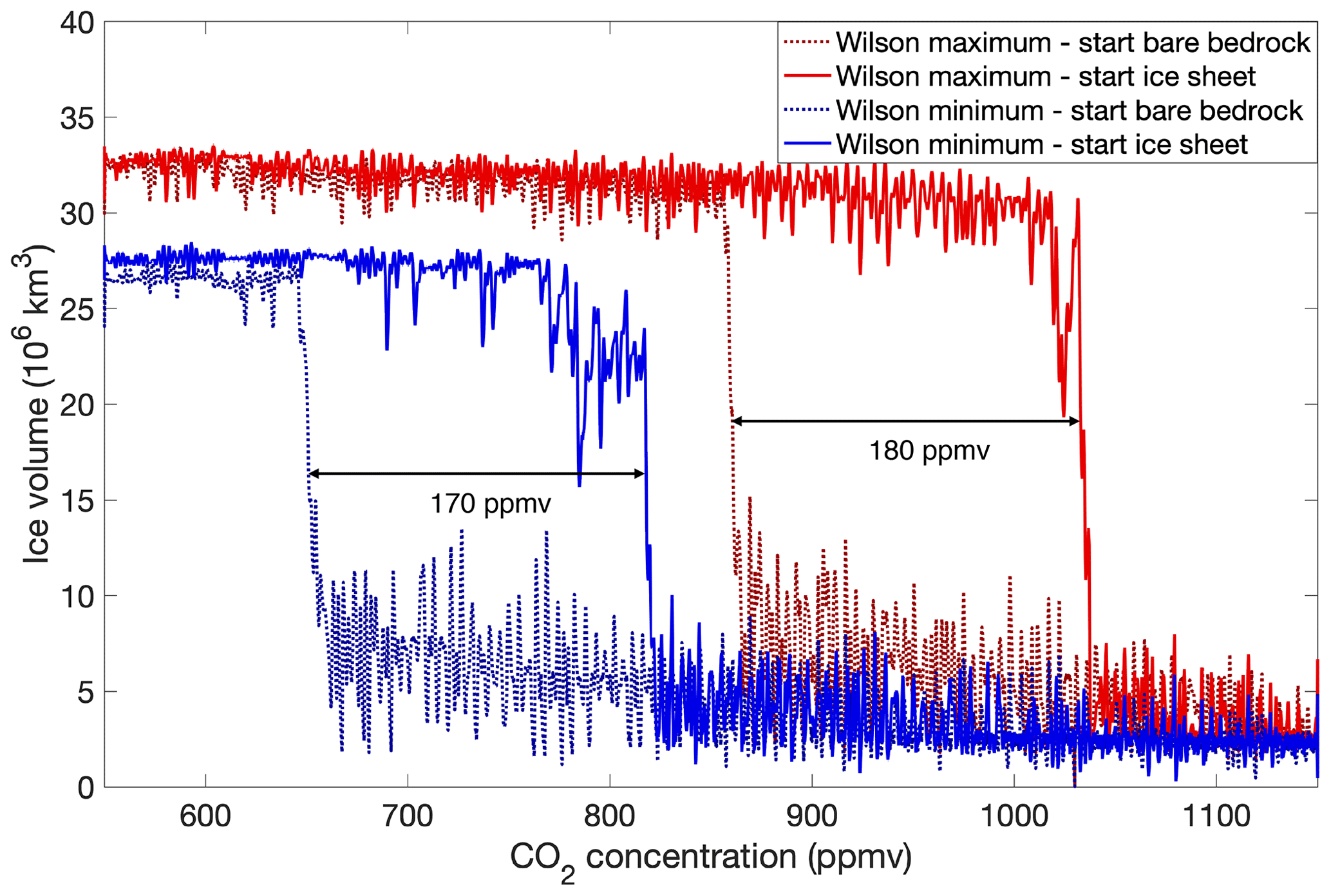
Figure 5Hysteresis behaviour of ice sheet growth and decline for linearly varying CO2 concentrations between 550 and 1150 ppmv for the Wilson maximum bedrock topography (red) and the Wilson minimum bedrock topography (blue) reconstructions. The dotted lines represent simulations that start from a bare bedrock topography. The solid lines represent simulations that start from a continental-scale ice sheet.
The difference between the glaciation and deglaciation thresholds can also be expressed in terms of a temperature change. Grounding line retreat for marine-based ice sheets can be initiated by subsurface melting of ice shelves, but melting of a continental-scale ice sheet is mostly governed by changes in the surface mass balance. Hence, the surface temperature is key in determining the threshold at which the ice sheet starts to grow or when the deglaciation occurs. MAT_sur defined for individual grid points ranges from −5 ∘C at the ice sheet margin to between −45 and −50 ∘C in East Antarctica for the Wilson minimum and Wilson maximum bedrock topography, respectively. The colder temperatures for the Wilson maximum topography are mainly due to the differences in surface elevation (Fig. 6). These temperatures are reached for a CO2 forcing of 550 ppmv and are still about 10–20 ∘C higher than the temperatures over the present-day Antarctic ice sheet.
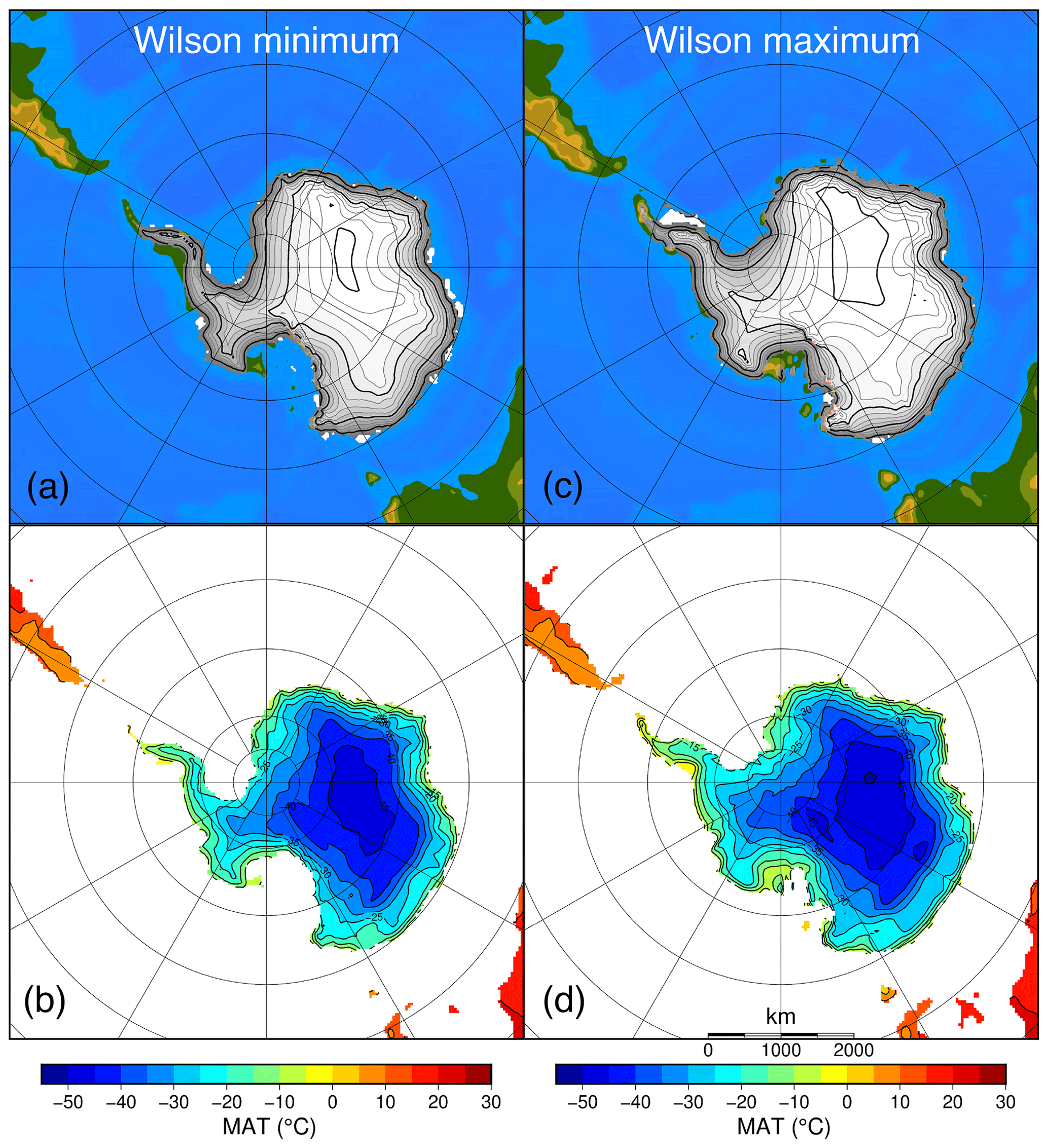
Figure 6Continental-scale ice sheet geometry for the (a) Wilson minimum bedrock topography and (b) the corresponding spatially varying mean annual surface temperature as well as for (c) the Wilson maximum bedrock topography and (d) the corresponding spatially varying mean annual surface temperature. Thin contour intervals are given every 250 m, while thick contour intervals are given each 1000 m for the ice sheet surface elevation.
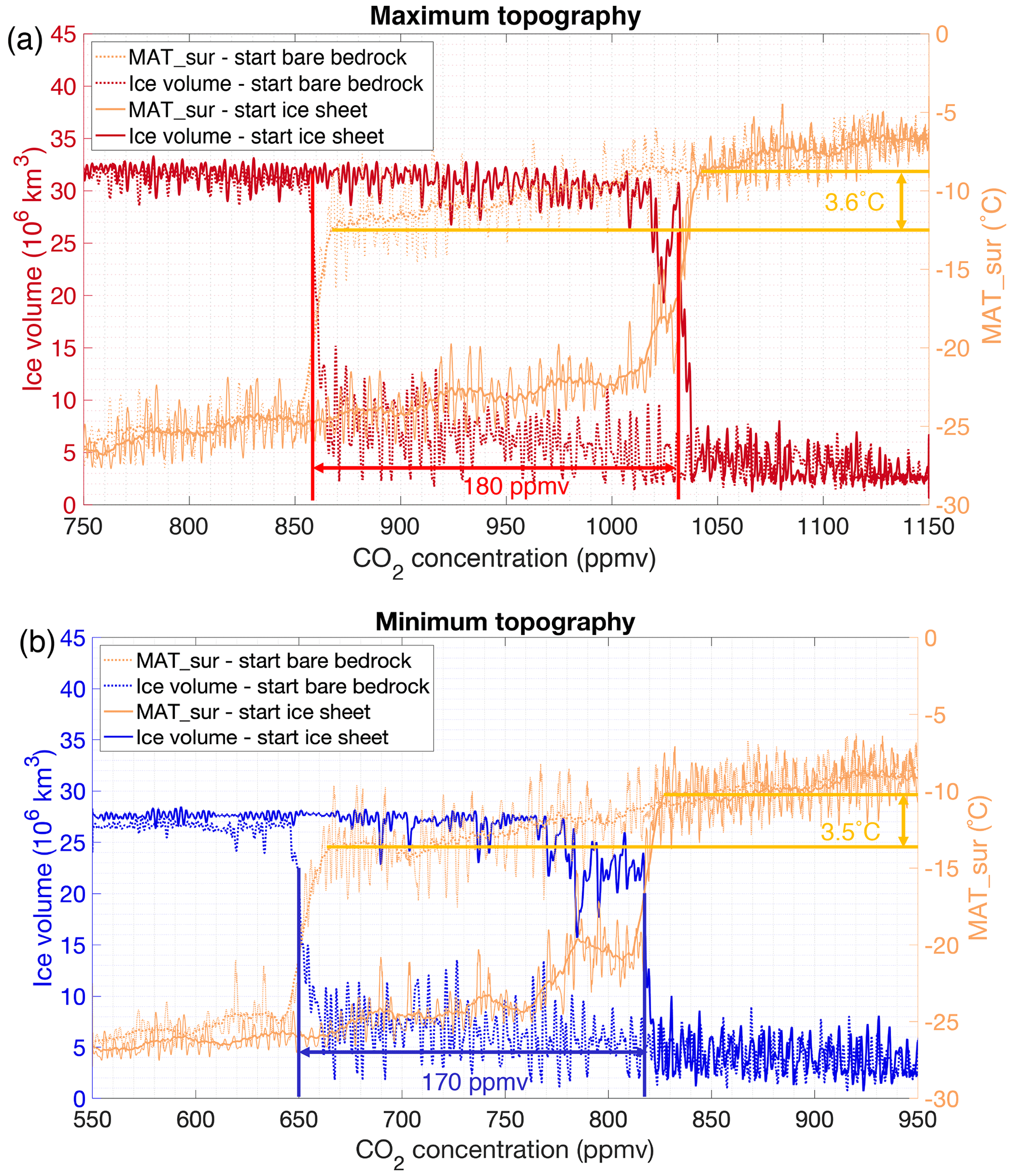
Figure 7Mean annual temperature change (MAT_sur) and ice volume evolution using (a) the Wilson maximum bedrock topography and (b) the Wilson minimum bedrock topography. The simulation starts either from a bare bedrock and a CO2 forcing of 1150 ppmv that linearly decreases towards 550 ppmv or from a continental-scale ice sheet and a CO2 forcing of 550 ppmv that linearly increases towards 1150 ppmv.
The MAT_sur for a deglaciated Antarctic continent at 1150 ppmv is about −7 ∘C during the late Eocene for the Wilson maximum bedrock topography (Fig. 7a) and slightly higher at −6 ∘C for the Wilson minimum bedrock topography (Fig. 7b). The annual range in temperatures is about 30 ∘C with a mean January temperature of 13 ∘C and a mean July temperature of −17 ∘C (not shown). This indicates that in wintertime snow accumulates, while it melts again in summer. The MAT_sur needs to be lower to cause a full glaciation by ∼6 and ∼8 ∘C for the Wilson maximum and minimum bedrock topographies, respectively. Temperatures range from −26 to −29 ∘C for the Wilson minimum and the Wilson maximum bedrock topography at a CO2 concentration of 550 ppmv for a fully glaciated continent. To make the transition back to a deglaciated continent, the MAT_sur needs to rise above −20 ∘C (Fig. 7).
For the Wilson minimum bedrock topography, the MAT_sur above the Antarctic continent is −14 ∘C when the entire continent is glaciated starting from a bare bedrock. Starting from a fully glaciated continent, the ice sheet deglaciates when the MAT_sur reaches −10 ∘C. For the Wilson maximum bedrock topography, these temperatures are very similar with a MAT_sur of −13 ∘C when the entire continent is glaciated starting from a bare bedrock and deglaciation starts when the MAT_sur reaches −9 ∘C. This again indicates that the hysteresis effect is quasi-independent of the particular bedrock elevation dataset. The hysteresis effect, expressed in terms of the MAT_sur threshold between glaciation and deglaciation, is about 4 ∘C.
3.2 Influence of isostasy
It is thought that isostatic adjustment provides a negative feedback to ice sheet growth. During the build-up of the ice sheet, the ice mass interacts with the lithosphere and deforms the underlying bedrock. Hence, the ice sheet elevation will not rise as fast and the increase in accumulation area (when the ice sheet's height exceeds the snowline) will be delayed. The magnitude of this feedback is determined by performing experiments in which isostatic adjustment is not considered.
The hysteresis effect in terms of the CO2 forcing is much less pronounced when isostasy is neglected. The ice sheet decline occurs for a similar threshold of about 1030 ppmv when isostatic adjustment is not taken into account (Fig. 8). This is mainly a consequence of the ice–albedo feedback that is similarly strong in the experiment with isostasy and without isostasy because the area of the continental-scale ice sheet is the same regardless of the inclusion of isostatic adjustment. The maximum height of the equilibrated continental-scale ice sheet is about 160 m higher without considering isostasy, while the ice thickness differences exceed 1000 m (Fig. S2). The small difference in surface elevation barely has an impact on the CO2 threshold to induce the deglaciation.
Without considering isostasy, the threshold towards full glaciation occurs at a CO2 concentration of 990 ppmv (compared to 850 ppmv for the simulation including isostasy) due to the more rapid increase in the surface elevation when snow accumulates. Aside from the higher surface elevation (up to 800 m higher) prior to the glaciation threshold, the ice sheet area is about twice the size when excluding isostasy. In this case, the hysteresis effect with respect to the CO2 forcing is only 40 ppmv. The MAT_sur threshold to glaciation is again about −13 ∘C, exactly the same temperature threshold as the experiment including isostasy. As already stated, this is a consequence of the increase in surface elevation when snow and ice accumulate. The deglaciated continent has a MAT_sur of −6 ∘C because of the smaller ice sheet extent and generally lower surface elevation (Fig. 9).
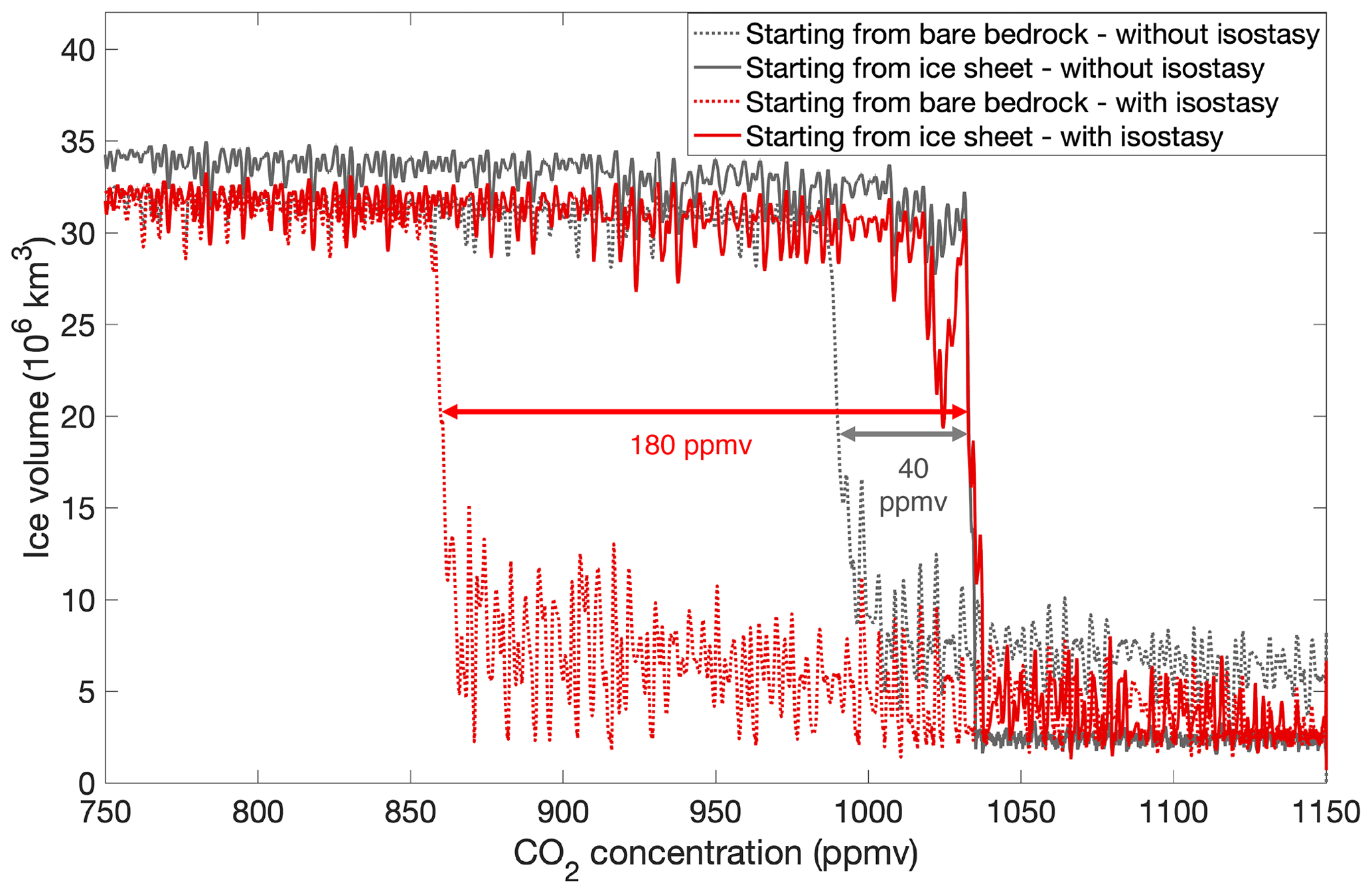
Figure 8Ice sheet growth and decline for linearly decreasing and increasing CO2 concentrations from 750 to 1150 ppmv for the Wilson maximum bedrock topography reconstruction. The grey lines represent the ice sheet evolution for the simulations excluding isostasy, and the red lines represent the ice sheet evolution with isostasy.
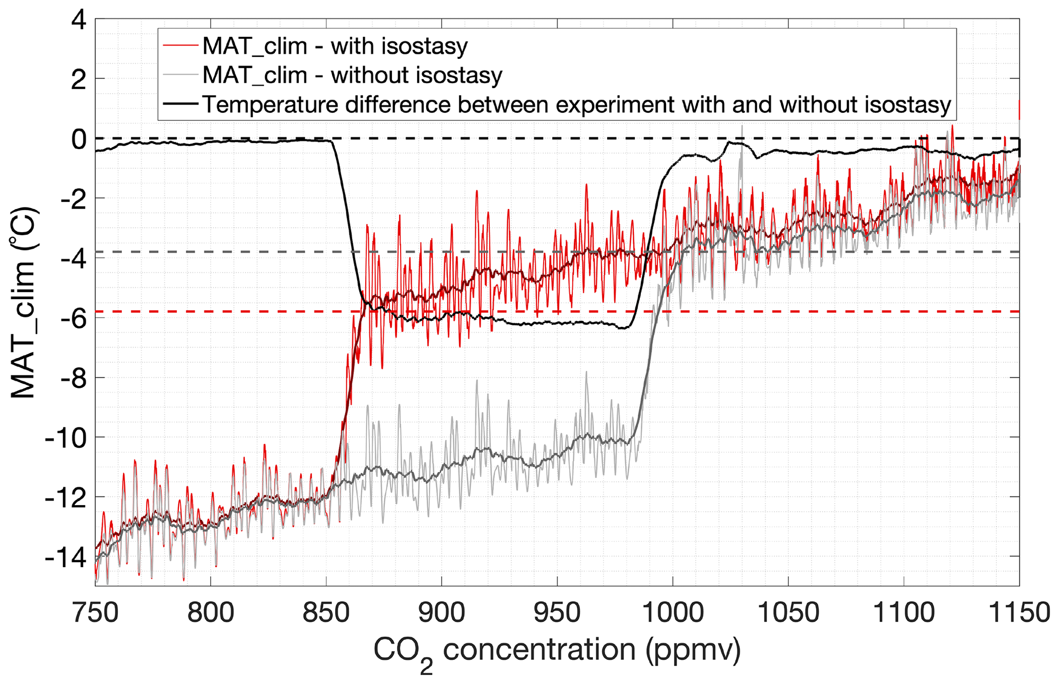
Figure 9Elevation-corrected mean annual temperature (MAT_clim) above the Antarctic continent. The simulations start from a bare bedrock and either include isostasy (red) or exclude isostasy (grey). The dashed black horizontal line indicates no temperature difference between the experiment including or excluding isostasy. The dashed red and grey horizontal lines indicate the MAT thresholds at which the Antarctic ice sheet grows to a continental scale.
The temperature threshold to glaciation and deglaciation is very similar for the experiments that include isostatic adjustment and those that exclude it. To disentangle the influence of surface elevation, the MAT_sur is now corrected for the surface elevation change by applying a constant lapse-rate correction in order to calculate the temperature at sea level, which we equate to the climatological mean annual temperature (MAT_clim). As it occurs, the initial temperature difference of about 0.5 ∘C between the two experiments with CO2 concentrations between 1000 and 1150 ppmv is due to the larger ice sheet area in the experiment that excludes isostasy. After the transition to a continental-scale ice sheet for a CO2 concentration below 850 ppmv, this difference between the two simulations is negligible because the area of the continental-scale ice sheet is ultimately bounded by the size of the Antarctic continent. The larger the ice sheet area, the more incoming solar radiation will be reflected and the lower the surface temperature will be. The difference in the elevation-corrected MAT_clim threshold to full glaciation is ∼2 ∘C (Fig. 9).
Ice sheet hysteresis occurs when a threshold in the forcing is crossed that leads to a self-amplifying positive feedback loop. On palaeoclimatic timescales on the order of 100 kyr and longer, this threshold is determined by changes in the carbon cycle (or changes in the atmospheric CO2 concentration) and variations in the orbital parameters. First, the influence of the eccentricity is evaluated because the eccentricity modulates the magnitude of the precession and hence determines the magnitude of a threshold (Sect. 4.1). Then, simulations are run to a steady state for a constant forcing for different orbital parameter combinations (Sect. 4.2).
4.1 Influence of the eccentricity
There is a different CO2 threshold to continental-scale glaciation for each tested bedrock topography. However, in a narrow range of CO2 concentrations, the glaciation threshold is also paced by the orbital parameters. Figure 10 shows the eccentricity thresholds to continental-scale glaciation for a constant CO2 forcing between 810 and 890 ppmv and the eccentricity thresholds for complete deglaciation for a CO2 forcing between 980 and 1060 ppmv. All simulations start with the same initial conditions, and the ice sheet volume responds to the orbital forcing (experiments (a) and (b) in Table 2). Throughout the 2.4 Myr long runs, the ice sheet geometry has changed at each eccentricity extremum (∼100 kyr, ∼400 kyr, ∼2.4 Myr) because the ice sheet size periodically reacts to the precession (∼20 kyr). The time axis indicates the time needed since the start of the simulations to reach the eccentricity threshold to glaciation or deglaciation. For atmospheric CO2 values below 810 ppmv, the ice sheet always reaches a continental scale when the eccentricity declines below 0.04. For CO2 values exceeding 890 ppmv, the ice sheet cannot grow to a continental scale, not even during a prolonged insolation minimum. In this narrow range of CO2 concentrations, the eccentricity has a large influence on the ice sheet initiation and stability. Starting from a bare bedrock, the ice sheet stops growing and either declines or stays with constant volume whenever the eccentricity exceeds a value of 0.05 and then grows again when eccentricity declines. The ice sheet can initially grow and vary with the precession for up to four cycles before the onset to full glaciation sets in, depending on the value of the eccentricity and the CO2 forcing (Fig. S3). This shows that it is not only the magnitude of the eccentricity that determines the timing of ice sheet growth, but also the initial size of the ice sheet that is determined by the ice sheet history. Even though the CO2 forcing is constant, the ice sheet grows to a fully glaciated state consecutively for a CO2 forcing of 850, 860, 870, 880 and 890 ppmv. The higher the CO2 concentration, the more the ice sheet needs to grow before the threshold to full glaciation is reached.
The extreme eccentricity value of 0.064 that occurs after 2 Myr is not sufficient to melt the ice sheet once it has grown to a continental scale for a CO2 forcing between 810 and 890 ppmv. This again shows the hysteresis effect of the Antarctic ice sheet: an eccentricity below 0.032 is enough to initiate continental-scale ice sheet growth for a CO2 forcing up to 890 ppmv, while an eccentricity of >0.06 is not sufficient to make the ice sheet melt entirely after this. The extreme eccentricity of 0.064 influences the ice sheet volume for all simulations forced with a constant CO2 concentration between 800 and 890 ppmv, but the peak insolation forced by the precessional cycle is too short-lived to melt the entire ice sheet (Fig. S3). Such extreme values of the eccentricity exceeding 0.06 only occur when the 100 kyr cycle, the 405 kyr cycle and the 2.4 Myr cycle reach a maximum. The absolute maximum in the eccentricity of 0.064 at 32.2 Ma and a minimum in the 2.4 Myr cycle around 33.4 Ma are captured in this interval, which is important for determining the respective thresholds to ice sheet decline and ice sheet growth.
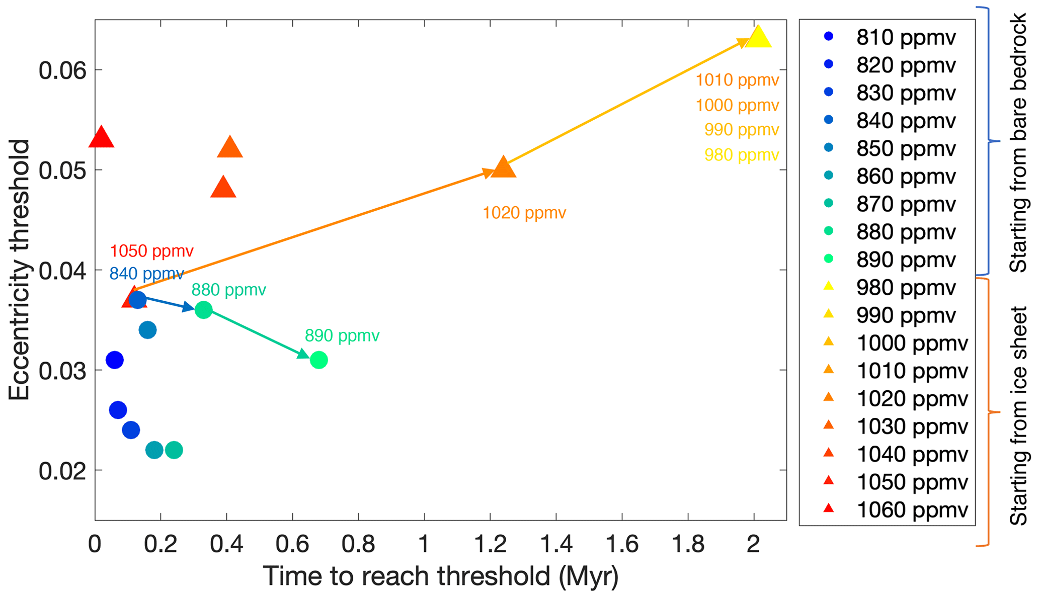
Figure 10Eccentricity thresholds for ice sheet initiation starting from a bare bedrock (blue to green dots) and eccentricity thresholds for ice sheet decline (red to yellow triangles) for a range of different CO2 values. The time on the x axis indicates the duration before the continental-scale ice sheet growth or the ice sheet decline initiates. The experiment duration has an influence on the initial size of the ice sheet before another threshold is reached. The blue and green arrows indicate the decrease in eccentricity threshold for increasing CO2 values to initiate glaciations. The orange and yellow arrows indicate the increase in the eccentricity threshold for decreasing CO2 values to end glaciations. The thresholds are determined using the Wilson maximum bedrock topography.
Starting from a fully glaciated continent, the CO2 threshold to complete deglaciation has a range between 980 and 1060 ppmv (Fig. 10). An eccentricity of >0.05 initiates ice sheet decline in a CO2 concentration range between 1020 and 1060 ppmv. Either a higher value for the eccentricity or a longer duration since the start of the experiments is needed to disintegrate the Antarctic ice sheet for lower CO2 values. The experiment duration has an influence on the initial size of the ice sheet. For instance, the eccentricity maximum of 0.051 at the start of the experiment was not high enough to make the Antarctic ice sheet disappear at a CO2 forcing of 1050 ppmv. However, the ice sheet declines during the next eccentricity maximum exceeding 0.038 for a CO2 forcing of 1050 ppmv, while it can regrow for a CO2 forcing of 1040 ppmv. This indicates that the CO2 and orbital parameter thresholds exhibit state dependency; the thresholds to glaciation or deglaciation differ depending on the initial size of the ice sheet. The extreme eccentricity of 0.064 also induces deglaciation at CO2 concentrations between 980 and 1010 ppmv.
4.2 Constant forcing runs for different orbital parameter combinations
So far, the hysteresis effect has been investigated with a time-dependent forcing. To further separate the effects of the orbital parameters and the CO2 thresholds on glaciation and deglaciation, a number of simulations are run to a steady state for a constant forcing. Three different summer insolation (daily mean for DJF at 65∘ S) values are selected to perform the steady-state runs: a relatively low summer insolation of 427 Wm−2 (further referred to as a “cold” orbital configuration), a relatively high summer insolation of 467 Wm−2 (further referred to as a “warm” orbital configuration) and an insolation value between these two extremes of 440 Wm−2 (Fig. 11). These insolation values can be achieved for different orbital parameter combinations but correspond here to the values given in Table 3. For comparison, the present-day austral summer insolation (daily mean for DJF at 65∘ S) is 439 Wm−2. The eccentricity and the obliquity values resemble the cold orbital configuration, but the Earth is in perihelion during the austral summer today. The cold orbital configuration is chosen as the maximum insolation in an interval of ∼40 kyr. This is about the time needed to grow a continental-scale ice sheet (Fig. 12). The summer insolation is much lower during shorter intervals of several millennia, but these intervals are too short to significantly increase the size of the Antarctic ice sheet and to induce a continental-scale glaciation. Figure 11 also indicates that a warm orbital configuration in Antarctica can be caused by either a high obliquity or a high eccentricity in combination with the Earth in perihelion. The highest peak in the summer insolation at 32.18 Ma occurs when both eccentricity and obliquity are high. The selected cold orbital configuration occurs at a time when the eccentricity reaches a minimum.
Table 3Austral summer insolation values, eccentricity and obliquity for the different selected orbital configurations. Present-day insolation values and orbital parameters (eccentricity and obliquity) are given for comparison.
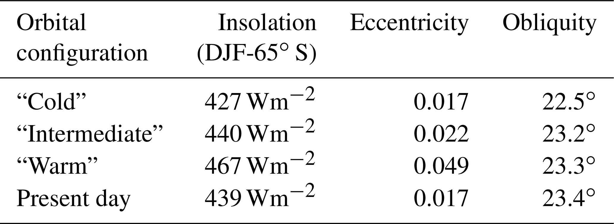
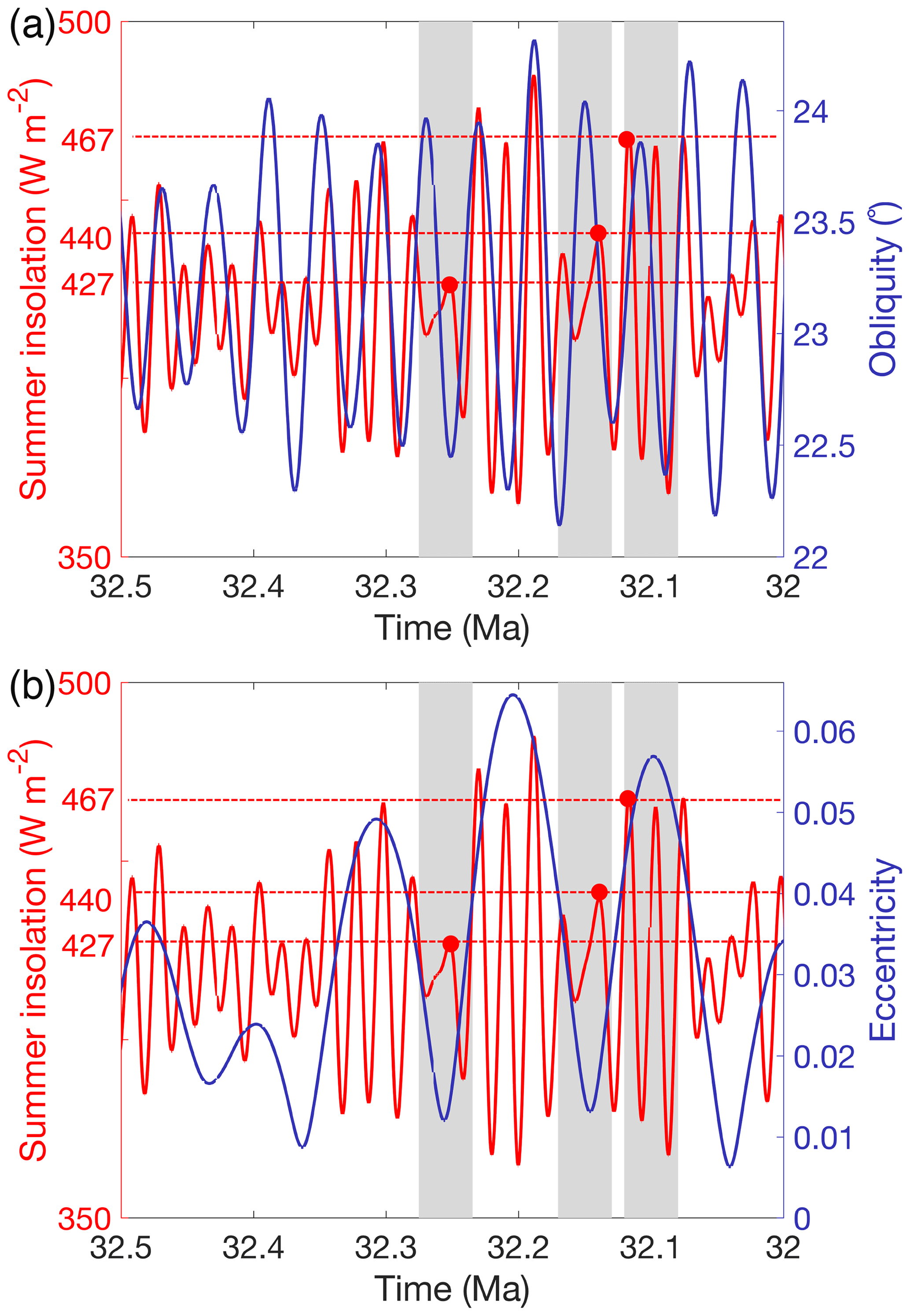
Figure 11Summer insolation variations at 65∘ S with respect to the (a) obliquity and (b) eccentricity. Three different summer insolation values are indicated by the red dots that indicate the maximum insolation during a 40 kyr interval (indicated by the grey shaded area). These three different insolation values are representative for a relative cold orbital configuration (427 Wm−2), an intermediate orbital configuration (440 Wm−2) and a warm orbital configuration (467 Wm−2).
Starting from a bare bedrock, the Antarctic ice sheet can grow to a continental scale for our cold orbital configuration for a CO2 forcing up to 850 ppmv (Fig. 12a). For an intermediate orbital configuration, the ice sheet can grow to a continental scale up to a CO2 forcing of 700 ppmv, and for a warm orbit, the ice sheet is never able to grow beyond a critical threshold to induce continental-scale ice sheet growth (not shown). Starting from a fully glaciated continent, the Antarctic ice sheet declines for a CO2 forcing of 1000 ppmv and higher (Fig. 12b). The ice sheet never completely deglaciates during a cold orbit or an intermediate orbit in the range of considered CO2 concentrations (not shown).
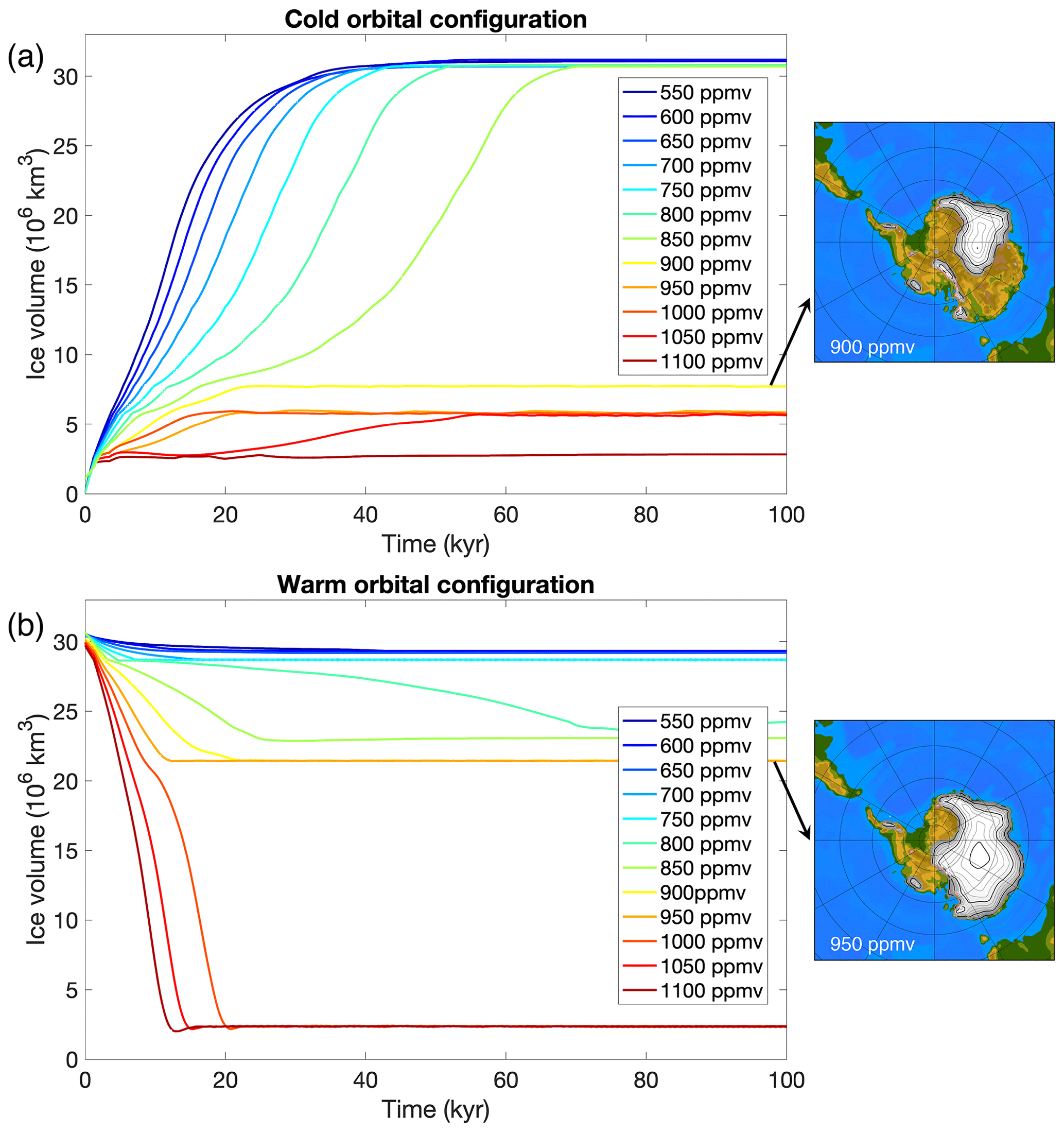
Figure 12Ice sheet evolution until steady state for different constant forcing scenarios. (a) A cold orbital configuration (summer insolation at 65∘ S of 427 Wm−2) and different CO2 concentrations at an interval of 50 ppmv starting from a bare bedrock. (b) A warm orbital configuration (summer insolation at 65∘ S of 467 Wm−2) and different CO2 concentrations at an interval of 50 ppmv starting from a fully glaciated continent. Ice sheet geometries are shown just before the tipping points are crossed at 900 ppmv for ice sheet growth (cold orbital configuration) and 950 ppmv for ice sheet decline (warm orbital configuration).
The timescales for growth and decline of a continental ice sheet reveal an asymmetry. It takes about 30–70 kyr to build up a continental-scale Antarctic ice sheet, while the ice sheet demise takes about 10–20 kyr. The ice sheet grows much faster to a continental scale for a CO2 forcing of 550 ppmv than for a CO2 forcing of 850 ppmv because the initial area of positive mass balance is much larger (Fig. 13). A CO2 concentration of 850 ppmv is close to the glaciation threshold and ice sheet–climate feedbacks are necessary to make the ice sheet grow. Initially, the ice sheet grows fast up to 18 kyr when the ice sheet volume change stagnates and increases again after 30 kyr when the ice sheet covers about one-third of the Antarctic continent and the ice–albedo and height–mass balance feedbacks reinforce the ice sheet growth. The highest mass balance rates occur along the ice sheet margin and range between 2–4 m yr−1 of accumulation. During the early stage of ice sheet build-up, the accumulation in the Gamburtsev Mountains goes up to 0.5 m yr−1, while it is around 2 m yr−1 in Dronning Maud Land. As the ice sheet grows, the accumulation lowers in central Antarctica, which is somehow similar to the situation at present due to the development of a high-pressure area, the decrease in surface air temperature with the depletion of its water vapour content and the orographic precipitation along the margin that depletes the air moisture further.
The “coldest” orbital configuration, which corresponds to the lowest austral summer insolation, occurs when the obliquity is low, the eccentricity is high and the Earth is in aphelion. The time-dependent results clearly suggest that the eccentricity must largely determine the ice sheet growth because the timescale to initiate continental-scale glaciation is longer than the period of the precession or obliquity for the higher CO2 concentrations. The CO2 threshold to induce a glaciation in a transient setting is therefore lower for high values of the eccentricity. Figure 14a shows the maximum ice sheet volume for simulations starting from a bare bedrock for a constant CO2 concentration and a constant eccentricity (while precession and obliquity vary; experiments (c) and (d) in Table 2). Figure 14b shows the maximum ice sheet volume for simulations starting from a bare bedrock for a constant CO2 concentration and a constant obliquity (while precession and eccentricity vary). Figure 14c and d show the minimum ice sheet volume for similar runs, but starting from a continental-scale ice sheet.
The higher the eccentricity, the lower the CO2 concentration to induce the deglaciation (Fig. 14c). On the other hand, for a given CO2 forcing below the glaciation threshold, the ice sheet can grow more for a higher eccentricity (Fig. 14a). The higher eccentricity modulates the precession, and for a high eccentricity the summer insolation minimum is lower when the Earth is in aphelion. As noted earlier, the duration of such a very low insolation minimum is not long enough to make the ice sheet grow on the entire Antarctic continent. Therefore, the CO2 concentration needs to drop more to initiate ice sheet growth at high eccentricity values. Figure 14 also illustrates this hysteresis behaviour, where the existence of a large ice sheet for a given forcing is dependent on the initial presence or absence of an ice sheet.
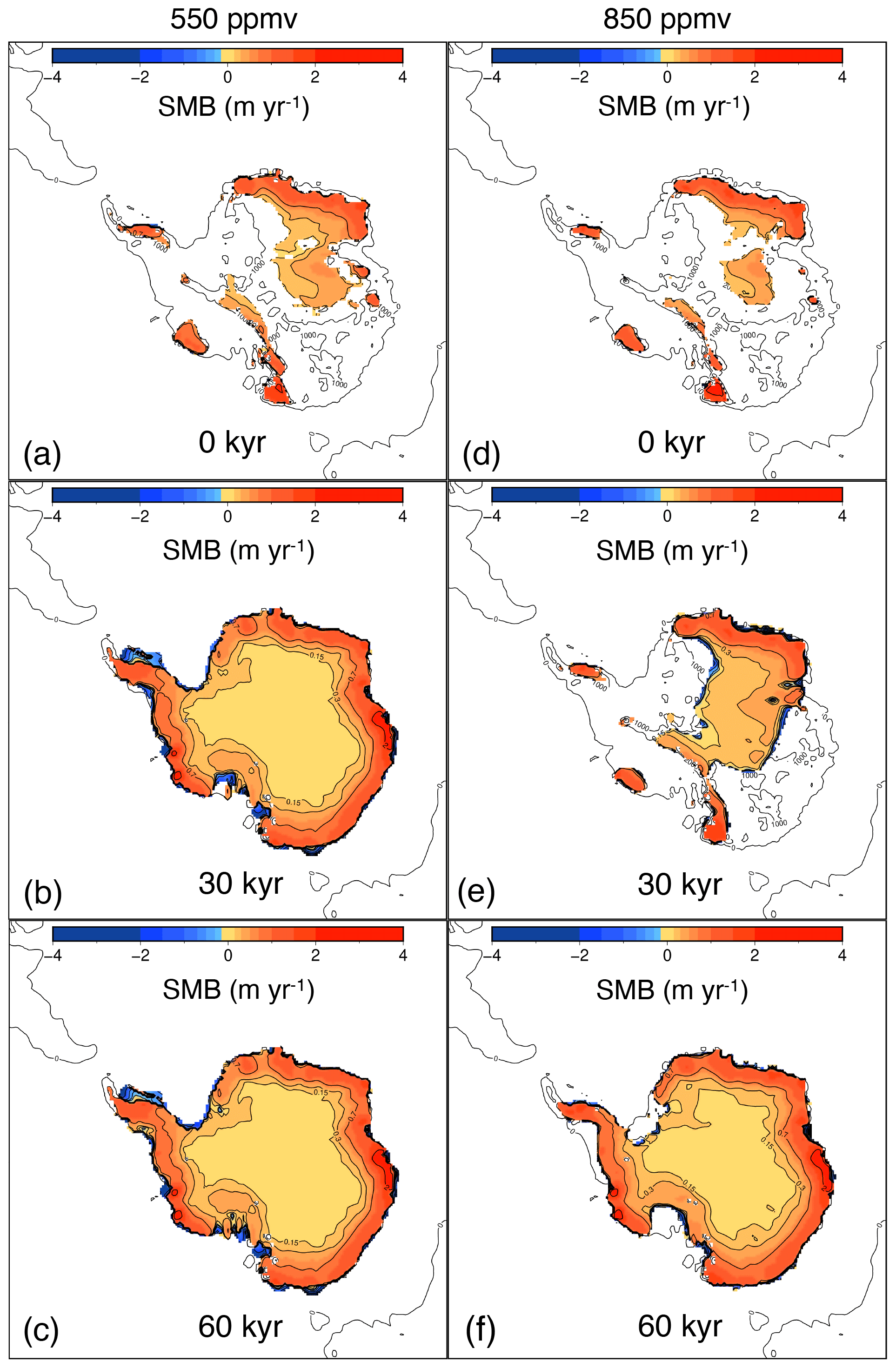
Figure 13Antarctic ice sheet surface mass balance (SMB) for the simulations starting from a bare bedrock forced by a cold orbital configuration and a CO2 concentration of 550 ppmv after (a) 0 kyr, (b) 30 kyr and (c) 60 kyr as well as a CO2 concentration of 850 ppmv after (d) 0 kyr, (e) 30 kyr and (f) 60 kyr.
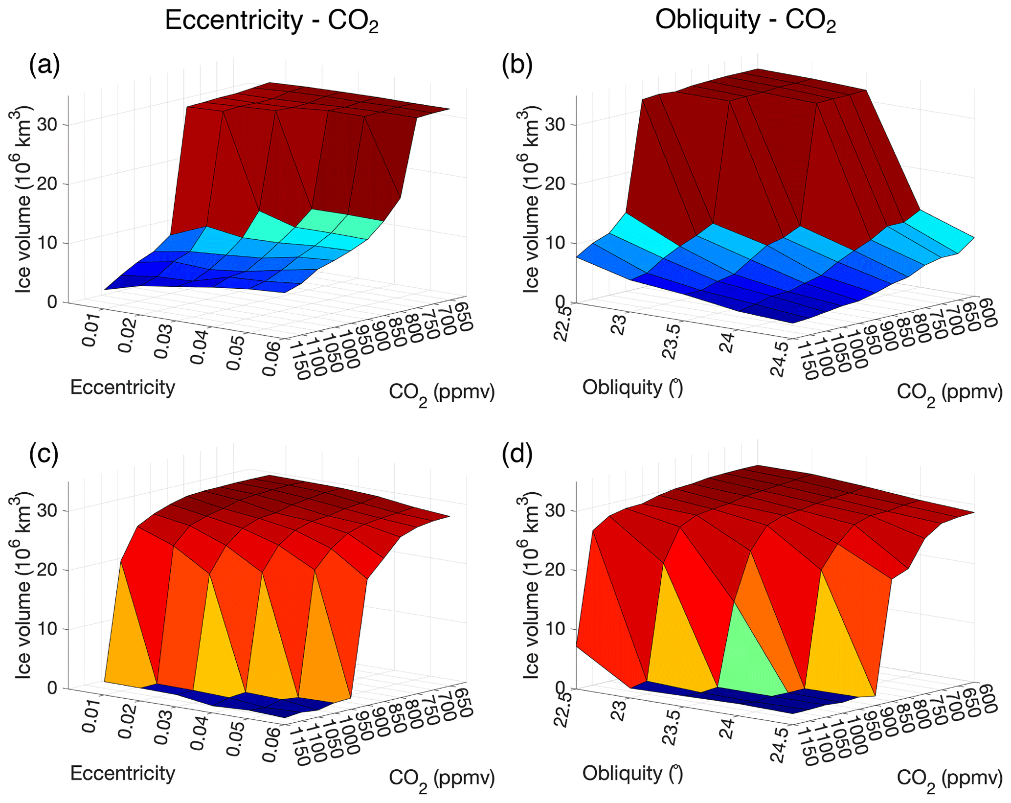
Figure 14Simulations starting from bare bedrock showing the maximum ice sheet volume for a range of CO2 concentrations between 600 and 1150 ppmv for (a) a constant eccentricity between 0.01 and 0.06 while precession and obliquity are variable as well as (b) a constant obliquity between 22.5 and 24.5∘ while precession and eccentricity are variable. Panels (c) and (d) are the same as (a) and (b), but the simulations start from a continental-scale ice sheet and the minimum ice sheet volume achieved during the run is shown.
Figure 14b shows the maximum ice sheet volume for simulations starting from a bare bedrock for a constant obliquity and a constant CO2 concentration, while Fig. 14d shows the minimum ice sheet volume for similar runs starting from a continental-scale ice sheet (see experiments (e) and (f) in Table 2). The lower values for the obliquity clearly favour glaciation. For a constant obliquity of 22.5∘, the ice sheet grows to a continental scale at 1000 ppmv, while for an obliquity of 24.5∘, the ice sheet never reaches the continental scale. For the simulations starting from a continental-scale ice sheet, the ice sheet never completely melts for a low obliquity of 22.5∘, not even for a high CO2 forcing of 1150 ppmv. This indicates that the role of the eccentricity for melting a large-scale ice sheet is only important during times when the obliquity is high. Looking at the transition between a glaciated and a deglaciated continent for a constant forcing, it is apparent that the ice sheet volume first gradually changes before a strong nonlinear feedback initiates. This effect is further investigated simulating steady-state ice sheet geometries for a range of temperature anomalies starting again from either an ice-free continent (bare bedrock) or an ice sheet (Fig. 15). Starting from the glaciated continent, first the ice sheet retreats with ∼40 % of the continental-scale ice sheet area before the nonlinear feedbacks are initiated. On the other hand, when starting from a bare bedrock, the steady-state ice sheet area first gradually increases when lowering the surface temperature until the continent is covered with approximately 40 % ice before a sharp transition occurs towards a fully glaciated continent.
Hysteresis behaviour related to the build-up and decline of ice sheets has a geometric cause (Oerlemans, 2002). The snowline must lower to allow for snow cover over the topography, initiating ice build-up. Obviously, the transition would be sharpest when the topography is flat and the snowline would intersect the entire topography at once. The lowering of the ice sheet surface during decay causes the atmospheric temperatures to rise even more because of the lapse rate and accelerates the melting process, a process named the height–mass balance feedback. Because ice sheet hysteresis has a geometrical origin, the initial height of the bedrock topography and the height of the continental-scale ice sheet are crucial to determine the thresholds for glaciation and deglaciation. We have confirmed that the CO2 thresholds and especially temperature thresholds to initiate and terminate glaciations differ depending on the height of the bedrock. These CO2 thresholds to initiate glaciations are 650 ppmv (minimum bedrock topography dataset) and 870 ppmv (maximum bedrock topography dataset). Aside from the bedrock dataset dependence, the thresholds also depend on the climate model used. As shown in Gasson et al. (2014), the thresholds may vary between 560 and 920 ppmv when climate model uncertainty is also included.
The hysteresis effect in our simulations has a magnitude of about 170–180 ppmv, slightly depending on the chosen bedrock topography dataset. CO2 variations had a magnitude of at least 170–180 ppmv during the late Eocene, or about 70 ppmv larger than the 110 ppmv glacial–interglacial CO2 variations of the Quaternary (Da et al., 2019). Given a sufficiently low CO2 level, this implies that Antarctic ice sheets could have also waxed and waned prior to the EOT. This was demonstrated in Van Breedam et al. (2022), who used a CO2 forcing based on available proxies that varied between 770 ppmv and >1200 ppmv at a low temporal resolution to investigate ephemeral glaciations during the late Eocene. Such CO2 variations are significantly larger than the hysteresis effect quantified in this study. One of the possible causes of the CO2 variations during the early Cenozoic could be the build-up of the ice sheet itself, which causes a positive feedback loop with increased ice volume, leading to lower CO2 levels and amplified glaciations (Ruddiman, 2006).
The transition towards a glaciated state occurs as a sudden, nonlinear response when the ice–albedo feedback and height–mass balance feedback reinforce the ice sheet growth at the threshold value. It is suggested that albedo feedbacks between the ice sheet and the climate increase the strength of the hysteresis. Pollard and DeConto (2005) found a hysteresis effect of about 100 ppmv at the EOT using a matrix look-up table with few initial ice sheet geometries that only roughly captured the ice–albedo feedback. Their hysteresis curves also showed a more stepwise change towards full glaciation and deglaciation, mainly because the height–mass balance feedback strengthens the ice sheet growth each time the topography is above the snowline, leading to a (partly) glaciated continent.
Our simulations indicate that the ice sheet–climate feedbacks cause rapid ice sheet expansion when the ice sheet covers about 40 % of the continent (Fig. 15). Conversely, the Antarctic ice sheet area needs to decrease by about 40 % (corresponding to an ice volume loss of 30 % of the grounded ice volume) to initiate rapid ice sheet decay. This is in line with estimates from Ridley et al. (2010), who stated that the ice–albedo feedback becomes very effective when the ice sheet volume loss is about 30 % for melting the present-day Greenland ice sheet. Mikolajewicz et al. (2007) found that a changing surface albedo when ice is melting increased the local temperatures by up to 10 ∘C in summertime. The sharp glacial–deglacial transitions are caused by both the ice–albedo feedback and the height–mass balance feedback, and it is thought that their impact on the surface temperatures is of equal magnitude (Ridley et al., 2005). Opposite to the sharp transition between glacial and deglacial states from our study, studies that neglect the ice–albedo feedback such as Huybrechts (1994) and Garbe et al. (2020) show a more gradual transition to a deglaciated continent. Therefore, these studies might also overestimate the temperature forcing needed to melt the present-day Antarctic ice sheet.
Isostatic adjustment acts as a negative feedback during the glaciation of the Antarctic continent. Our simulations show that the strength of this feedback is quite large and lowers the CO2 threshold to continental-scale glaciations by about 130 ppmv. Oerlemans (2002) initially stated that the influence of isostatic movements should be small because the glaciation threshold occurs when the ice sheet is still small. However, our simulations indicate that the combined effect of a higher surface elevation and more extensive albedo changes due to a larger area makes a substantial difference in the glaciation threshold. During deglaciation, our simulations have indicated no significant impact of isostasy on the threshold to deglaciation. Isostatic uplift would reduce ice sheet melt, but the delayed response of the bedrock to changes in ice loading is too slow to counteract the increasing snowline (Abe-Ouchi et al., 2013). For the present-day Antarctic ice sheet, isostatic adjustment has had a stabilizing effect on the Antarctic ice sheet evolution since at least the last 10 kyr (Kingslake et al., 2018). Also, for future projections of the Antarctic ice sheet on multi-centennial timescales, the uplift provides a negative feedback to future West Antarctic ice sheet loss through grounding line stabilization (Larour et al., 2019).
An interesting thought experiment is to assess the sensitivity of the early Cenozoic Antarctic ice sheet subject to the present-day orbital forcing (e=0.0167, ε=23.4393 and ϖ=102.9179; J2000; Laskar et al., 2004) and a pre-industrial CO2 concentration of 280 ppmv. At present, the Earth is close to perihelion during the austral summer, a precondition to have high summer insolation values. Because of the low value of the eccentricity, the high summer insolation is attenuated and has a mean value for the austral summer at 65∘ S of 439 Wm−2. This is exactly in the middle between the selected “warm” and “cold” orbital configuration at the EOT. Imposing present-day orbital and CO2 forcing leads to surface temperatures that are still up to 10 ∘C warmer around Dome A compared to the present-day Antarctic ice sheet (Fig. S4). That is because in the early Cenozoic the location was less poleward than today. Prior to 22 Ma, the continental configuration also did not allow for the development of a strong circumpolar current (Evangelinos et al., 2022), but the full consequences of that are not assessed in the current set-up of the climate model with only a mixed-layer ocean. The threshold to glaciation for a model run starting from a bare bedrock occurs at a temperature perturbation of +2.6 ∘C, and the threshold to deglaciation occurs at a temperature perturbation of +7.6 ∘C (Fig. S5). This is somewhat lower than the +10 ∘C found by Garbe et al. (2020) to melt the present-day Antarctic ice sheet on account of the different continental and climatic setting of the Eocene and processes taken into account (ice–albedo feedback). Also, in contrast to the present-day Antarctic ice sheet, the early Cenozoic Antarctic ice sheet is largely grounded above sea level.
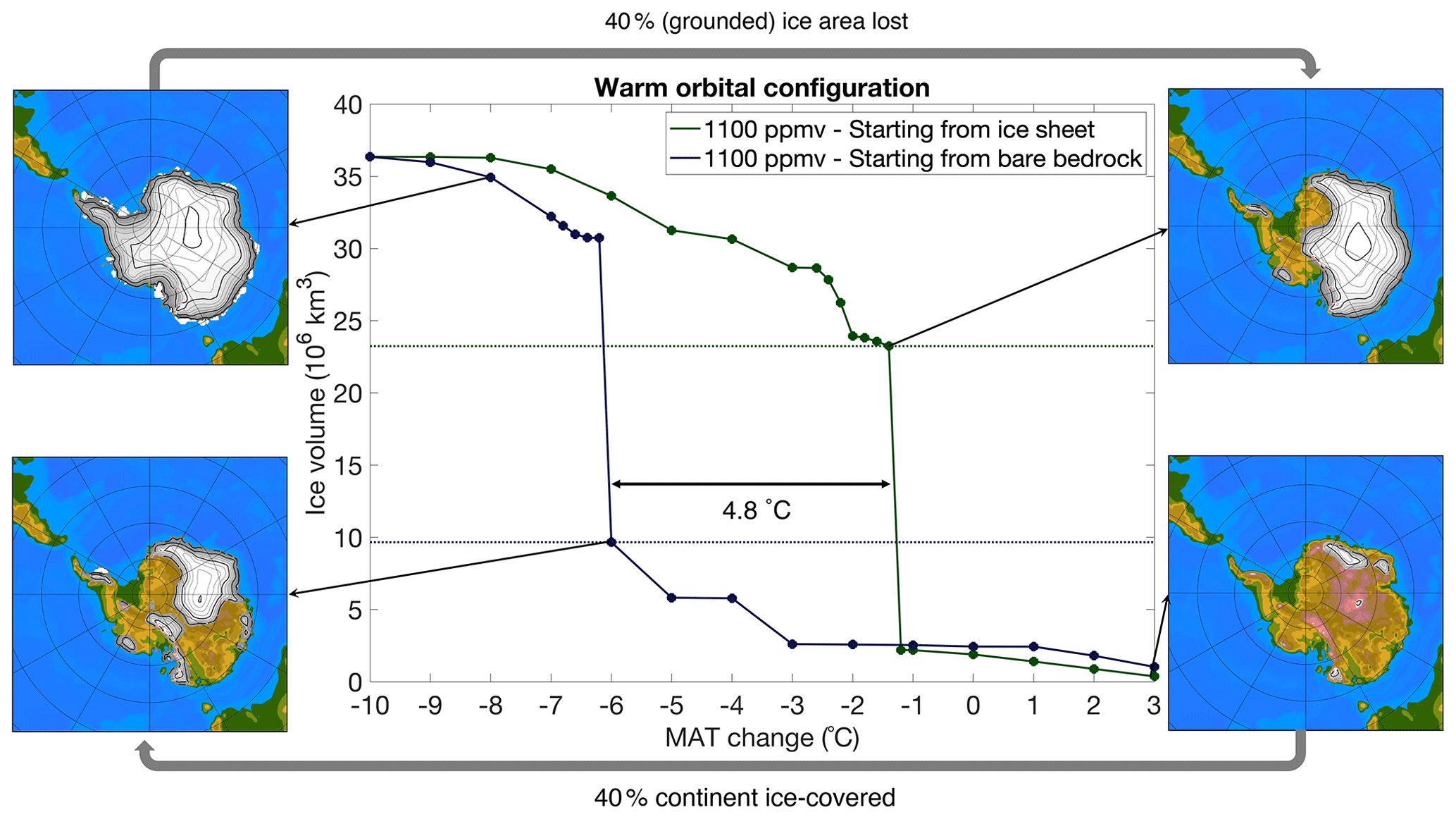
Figure 15Steady-state ice sheet volume for a range of mean annual temperature perturbation thresholds for ice sheet growth and decline for a warm orbital configuration of 467 Wm−2 at 65∘ S and a constant CO2 concentration of 1100 ppmv. The dotted green horizontal line indicates the ice sheet volume at which the strong nonlinear ice sheet decline initiates. The ice sheet volume at which a strong nonlinear increase ice sheet growth initiates is indicated by the dotted blue horizontal line. Snapshots of the ice sheet geometry are given at the tipping points. Thin contour intervals are given every 250 m, while thick contour intervals are given each 1000 m.
Nonlinear ice sheet dynamics are also triggered by the orbital parameters. The eccentricity has a main influence on the initiation and termination of glaciations on the Antarctic continent with initiation during eccentricity minima and terminations during eccentricity maxima. This is perhaps puzzling at first because the eccentricity only influences the forcing by modulating the precession. However, because the ice sheet decline depends on crossing a threshold value, the amplitude of the precession cycle becomes important and is governed by the eccentricity. Large values for the eccentricity result in a very low summer insolation during austral summer when the Earth is in aphelion and a very high summer insolation during austral summer when the Earth is in perihelion. To build a continental-scale Antarctic ice sheet, the role of the eccentricity is important in order to keep the amplitude of the precession low. Abe-Ouchi and Blatter (1993) have already indicated that the periods of precession (∼20 kyr) and obliquity (∼40 kyr) are too short to build up large ice sheets when the accumulation rate is low, and therefore eccentricity has to be low to prevent the summer insolation to peak when the Earth is in perihelion.
Despite the performance of a substantial number of sensitivity experiments related to the orbital and CO2 forcing, we did not perform a sensitivity analysis of the ice sheet parameter uncertainty. Ice sheet model parameters such as the enhancement factor, the basal sliding coefficient and the flow rate factor each have their uncertainty, and they are tuned to reproduce the present-day Antarctic ice sheet. Also, the parameters related to the isostatic model are not explored. For instance, the relaxation time of the asthenosphere and the flexural rigidity of the lithosphere add another degree of freedom. The most important parameters influencing ice sheet–climate model feedbacks are, however, parameters related to the albedo (Gandy et al., 2023). Because our modelling approach on very long timescales significantly improved the representation of albedo changes resulting from changes in the ice sheet extent (Van Breedam et al., 2021a), we believe that the ice sheet parameter uncertainty is of secondary importance here.
We have shown that the early Cenozoic Antarctic ice sheet grew nonlinearly during the late Eocene to Oligocene, when thresholds in the climate system were crossed. These thresholds at which glaciation occurs depend on boundary conditions such as the bedrock elevation. The CO2 threshold to glaciation is ∼650 ppmv for the minimum bedrock elevation and ∼870 ppmv for the maximum bedrock elevation datasets used in this study. The hysteresis behaviour of ice sheets arises because of the positive feedbacks associated with ice sheet growth and decline such as the elevation–surface mass balance feedback and the ice–albedo feedback. The Antarctic ice sheet hysteresis effect is independent of the specific bedrock elevation dataset and is ∼180 ppmv or equivalent to a 4 to 5 ∘C regional mean annual temperature change. Our simulations indicate the need to include ice–albedo feedbacks when the ice sheet is replaced by tundra during ice sheet melting and oppositely during ice sheet growth. The rapid transition between glacial and deglacial states as found in our simulations is attributed to this ice–albedo feedback and sets in when the Antarctic continent covers about 40 % of the area (threshold to glaciation) or when the ice area decreases with 40 % of the total ice area (threshold to deglaciation).
An important stabilizing feedback is the isostatic depression of the bedrock when the ice sheet is building up. When the ice sheet is growing, the bedrock is depressed because of the weight of the overlying ice and the surface elevation is lowered. When this feedback is neglected, the ice sheet grows much faster to a continental scale and the hysteresis effect is significantly weaker. We found that this feedback is significant because of both an increased surface elevation and a larger ice sheet accumulation area that lowers the surface albedo.
The orbital parameters might regulate ice sheet growth and decline close to the CO2 threshold for continental-scale (de)glaciation. The role of eccentricity is especially important because ice sheet growth operates on a timescale of 30–70 kyr (longer than the precession and obliquity cycles) and ice sheet decline is initiated by crossing a threshold where the eccentricity determines the magnitude of this threshold value. The orbital parameters trigger both glaciations and deglaciations in a CO2 range of ∼80 ppmv, where the ice sheet develops rapidly when the ∼100 kyr eccentricity cycle reaches a minimum (810–830 ppmv), the ∼400 kyr eccentricity cycle reaches a minimum (850–880 ppmv) or the ∼2.4 Myr eccentricity cycle reaches a minimum (890 ppmv) using the maximum bedrock topography dataset.
The model code from CLISEMv1.0, used to provide the climate forcing, is available at https://doi.org/10.5281/zenodo.5245156 (Van Breedam et al., 2021b).
The bedrock topography datasets used as boundary conditions in this study can be accessed at https://doi.org/10.5281/zenodo.10359835 (Van Breedam, 2023). All model output data are available upon request.
The supplement related to this article is available online at: https://doi.org/10.5194/cp-19-2551-2023-supplement.
JVB designed the coupling method between the emulator and the ice sheet model, designed the experimental set-up, and performed the simulations. MC developed the Gaussian process emulator. PH developed the ice sheet model code and provided guidance during the research. JVB wrote the paper with contributions from all co-authors.
The contact author has declared that none of the authors has any competing interests.
Publisher's note: Copernicus Publications remains neutral with regard to jurisdictional claims made in the text, published maps, institutional affiliations, or any other geographical representation in this paper. While Copernicus Publications makes every effort to include appropriate place names, the final responsibility lies with the authors.
We thank two anonymous reviewers for their useful comments and very detailed feedback.
This research has been supported by the Research Foundation Flanders (FWO Vlaanderen) with grant no. G091820N.
This paper was edited by Irina Rogozhina and reviewed by two anonymous referees.
Abe-Ouchi, A. and Blatter, H.: On the initiation of ice sheets, Ann. Glaciol., 18, 203–207, https://doi.org/10.3189/S0260305500011514, 1993.
Abe-Ouchi, A., Saito, F., Kawamura, K., Raymo, M. E., Okuno, J., Takahashi, K., and Blatter, H.: Insolation-driven 100,000 year glacial cycles and hysteresis of ice-sheet volume, Nature, 500, 190–193, https://doi.org/10.1038/nature12374, 2013.
Armstrong McKay, D. I., Staal, A., Abrams, J. F., Winkelmann, R., Sakschewski, B., Loriani, S., Fetzer, I., Cornell, S. E., Rockström, J., and Lenton, T. M.: Exceeding 1.5 ∘C global warming could trigger multiple climate tipping points, Science, 377, 1171, https://doi.org/10.1126/science.abn7950, 2022.
Baatsen, M., van Hinsbergen, D. J. J., von der Heydt, A. S., Dijkstra, H. A., Sluijs, A., Abels, H. A., and Bijl, P. K.: Reconstructing geographical boundary conditions for palaeoclimate modelling during the Cenozoic, Clim. Past, 12, 1635–1644, https://doi.org/10.5194/cp-12-1635-2016, 2016.
Baatsen, M., von der Heydt, A. S., Huber, M., Kliphuis, M. A., Bijl, P. K., Sluijs, A., and Dijkstra, H. A.: The middle to late Eocene greenhouse climate modelled using the CESM 1.0.5, Clim. Past, 16, 2573–2597, https://doi.org/10.5194/cp-16-2573-2020, 2020.
Boers, N. and Rypdal, M.: Critical slowing down suggests that the western Greenland Ice Sheet is close to a tipping point, P. Natl. Acad. Sci. USA, 118, e2024192118, https://doi.org/10.1073/pnas.2024192118, 2021.
Burgard, C., Jourdain, N. C., Reese, R., Jenkins, A., and Mathiot, P.: An assessment of basal melt parameterisations for Antarctic ice shelves, The Cryosphere, 16, 4931–4975, https://doi.org/10.5194/tc-16-4931-2022, 2022.
Calov, R. and Ganopolski, A.: Multistability and hysteresis in the climate-cryosphere system under orbital forcing, Geophys. Res. Lett., 32, L21717, https://doi.org/10.1029/2005GL024518, 2005.
Carter, A., Roley, T., R., Hillenbrand, C.-D., and Rittner, M.: Widespread Antarctic glaciation during the Late Eocene, Earth Planet. Sci. Lett., 458, 49–57, https://doi.org/10.1016/j.epsl.2016.10.045, 2017.
Cox, P. M., Betts, R. A., Bunton, C. B., Essery, R. L. H., Rowntree, P. R., and Smith. J.: The impact of new land surface physics on the GCM simulation of climate and climate sensitivity, Clim. Dynam., 15, 183–203, https://doi.org/10.1007/s003820050276, 1999.
Crucifix, M., Loutre, M. F., Lambeck, K., and Berger A.: Effect of isostatic rebound on modelled ice volume variations during the last 200 kyr, Earth Planet. Sc. Lett., 184, 623–633, https://doi.org/10.1016/S0012-821X(00)00361-7, 2001.
Da, J., Zhang, Y. G., Li, G., Meng, X., and Ji, J.: Low CO2 levels of the entire Pleistocene epoch, Nat. Commun., 10, 4342, https://doi.org/10.1038/s41467-019-12357-5, 2019.
De Vleeschouwer, D., Da Silva, A. C., Sinnesael, M., Chen, D., Day, J. E., Whalen, M. T., Guo, Z., and Claeys, P.: Timing and pacing of the Late Devonian mass extinction event regulated by eccentricity and obliquity, Nat. Commun., 8, 2268, https://doi.org/10.1038/s41467-017-02407-1, 2017.
Evangelinos, D., Escutia, C., van de Flierdt, T., Valero, L., Flores, J.-A., Harwood, D. M., Hoem, F. S., Bijl, P., Etourneau, J., Kreissig, K., Nilsson-Kerr, K., Holder, L., López-Quirós, A., and Salabarnada, A.: Absence of a strong, deep-reaching Antarctic Circumpolar Current zonal flow across the Tasmanian gateway during the Oligocene to early Miocene, Global Planet. Change, 208, 103718, https://doi.org/10.1016/j.gloplacha.2020.103221, 2022.
Evans, D., Sagoo, N., Renema, W., Cotton, L. J., Müller, W., Todd, J. A., Saraswati, P. K., Stassen, P., Ziegler, M., Pearson, P. N., Valdes, P. J., and Affek, H. P.: Eocene green- house climate revealed by coupled clumped isotope-Mg Ca thermometry, P. Natl. Acad. Sci. USA, 115, 1174–1179, https://doi.org/10.1073/pnas.1714744115, 2018.
Garbe, J., Albrecht, T., Levermann, A., Donges, J. F., and Winkelmann, R.: The hysteresis of the Antarctic Ice Sheet, Nature, 585, 538–544, https://doi.org/10.1038/s41586-020-2727-5, 2020.
Gandy, N., Astfalck, L. C., Gregoire, L. J., Ivanovic, R. F., Patterson, V. L., Sheriff-Tadano, S., Smith, R. S., Williamson, D., and Rigby, R.: De-Tuning Albedo Parameters in a Coupled Climate Ice Sheet Model to Simulate the North American Ice Sheet at the Last Glacial Maximum, J. Geophys. Res.-Earth, 128, e2023JF007250, https://doi.org/10.1029/2023JF007250, 2023.
Gasson, E., Lunt, D. J., DeConto, R., Goldner, A., Heinemann, M., Huber, M., LeGrande, A. N., Pollard, D., Sagoo, N., Siddall, M., Winguth, A., and Valdes, P. J.: Uncertainties in the modelled CO2 threshold for Antarctic glaciation, Clim. Past, 10, 451–466, https://doi.org/10.5194/cp-10-451-2014, 2014.
Herrington, A. R. and Poulsen, C. J.: Terminating the Last Interglacial: The Role of Ice Sheet-Climate Feedbacks in a GCM Asynchronously Coupled to an Ice Sheet Model, J. Climate, 25, 1871–1882, https://doi.org/10.1175/JCLI-D-11-00218.1, 2011.
Horton, D. E., Poulsen, C. J., Montañez, I. P., and DiMichele, W. A.: Eccentricity-paced late Paleozoic climate change, Palaeogeogr. Palaeocl., 331–332, 150–161, https://doi.org/10.1016/j.palaeo.2012.03.014, 2012.
Houben, A. J. P., Bijl, P. K., Sluijs, A., Schouten, S., and Brinkhuis, H.: Late Eocene Southern Ocean cooling and invigoration of circulation preconditioned Antarctica for full-scale glaciation, Geochem. Geophy. Geosy., 20, 2214–2234, https://doi.org/10.1029/2019GC008182, 2019.
Huybrechts, P.: Formation and disintegration of the Antarctic ice sheet, Ann. Glaciol., 20, 336–340, https://doi.org/10.3189/1994AoG20-1-336-340, 1994.
Huybrechts, P.: Sea-level changes at the LGM from ice-dynamic reconstructions of the Greenland and Antarctic ice sheets during the glacial cycles, Quaternary Sci. Rev., 21, 203–231, https://doi.org/10.1016/S0277-3791(01)00082-8, 2002.
Huybrechts, P. and De Wolde, J.: The Dynamic Response of the Greenland and Antarctic Ice Sheets to Multiple-Century Climatic Warming, J. Climate, 12, 2169–2188, https://doi.org/10.1175/1520-0442(1999)012<2169:tdrotg>2.0.co;2, 1999.
Janssens, I. and Huybrechts, P.: The treatment of meltwater retention in mass-balance parameterizations of the Greenland ice sheet, Ann. Glaciol, 31, 133–140, https://doi.org/10.3189/172756400781819941, 2000.
Kennett, J. P.: Cenozoic evolution of Antarctic glaciation, the circum-Antarctic Ocean, and their impact on global paleoceanography, J. Geophys. Res., 82, 3843–3860, https://doi.org/10.1029/JC082i027p03843, 1977.
Kingslake, J., Scherer, R. P., Albrecht, T., Coenen, J., Powell, R. D., Reese, R., Stansell, N. D., Tulaczyk, S., Wearing, M. G., and Whitehouse, P. L.: Extensive retreat and re-advance of the West Antarctic Ice Sheet during the Holocene, Nature, 558, 430–434, https://doi.org/10.1038/s41586-018-0208-x, 2018.
Klose, A. K., Karle, V., Winkelmann, R., and Donges, J. F.: Emergence of cascading dynamics in interacting tipping elements of ecology and climate, R. Soc. Open Sci., 7, 200599, https://doi.org/10.1098/rsos.200599, 2020.
Larour, E., Seroussi, H., Adhikari, S., Ivins, E., Caron, L., Morlighem, M., and Schlegel, N.: Slowdown in Antarctic mass loss from Solid Earth and sea-level feedbacks, Science, 364, eaav7908, https://doi.org/10.1126/science.aav7908, 2019.
Laskar, J., Robutel, P., Joutel, F., Gastineau, M., Correia, A. C. M., and Levrard, B.: A long-term numerical solution for the insolation quantities of the Earth, Astron. Astrophys., 428, 261–285, https://doi.org/10.1051/0004-6361:20041335, 2004.
Laskar, J., Fienga, A., Gastineau, M., and Manche, H.: La2010: a new orbital solution for the long-term motion of the Earth, Astron. Astrophys., 532, A89, https://doi.org/10.1051/0004-6361/201116836, 2011.
Le Meur, E. and Huybrechts, P.: A comparison of different ways of dealing with isostasy: examples from modelling the Antarctic ice sheet during the last glacial cycle, Ann. Glaciol., 23, 309–317, https://doi.org/10.3189/S0260305500013586, 1996.
Lenton, T., Rockström, J., Gaffney, O., Rahmstorf, S., Richardson, K., Steffen, W., and Schellnhuber, H. J.: Climate tipping points – too risky to bet against, Nature, 575, 592–595, https://doi.org/10.1038/d41586-019-03595-0, 2019.
Letréguilly, A., Huybrechts, P., and Reeh, N.: Steady-state characteristics of the Greenland ice sheet under different climates, J. Glaciol., 37, 149–157, https://doi.org/10.3189/S0022143000042908, 1991.
Levermann, A. and Winkelmann, R.: A simple equation for the melt elevation feedback of ice sheets, The Cryosphere, 10, 1799–1807, https://doi.org/10.5194/tc-10-1799-2016, 2016.
Li, Q., Marshall, J., Rye, C. D., Romanou, A., Rind, D., and Kelley, M.: Global Climate Impacts of Greenland and Antarctic Meltwater: A Comparative Study, J. Climate, 36, 3571–3590, https://doi.org/10.1175/JCLI-D-22-0433.1, 2023.
Mikolajewicz, U., Vizcaíno, M., Jungclaus, J., and Schurgers, G.: Effect of ice sheet interactions in anthropogenic climate change simulations, Geophys. Res. Lett., 34, L18706, https://doi.org/10.1029/2007GL031173, 2007.
Mitchell, R. N., Gernon, T. M., Cox, G. M., Nordsvan, A. R., Kirscher, U., Xuan, C., Liu, Y., and He, X.: Orbital forcing of ice sheets during snowball Earth, Nat. Commun., 12, 4187, https://doi.org/10.1038/s41467-021-24439-4, 2021.
Oerlemans, J.: On glacial inception and orography, Quatern. Int., 95–96, 5–10, https://doi.org/10.1016/S1040-6182(02)00022-8, 2002.
Pagani, M., Huber, M., Zhonghui, L., Bohaty, S. M., Henderiks, J., Sijp, W., Krishnan, S., and DeConto, R. M.: The Role of Carbon Dioxide During the Onset of Antarctic Glaciation, Science, 334, 1261–1264, https://doi.org/10.1126/science.1203909, 2011.
Pollard, D. and DeConto, R. M.: Hysteresis in Cenozoic Antarctic ice-sheet variations, Global Planet. Change, 45, 21, https://doi.org/10.1016/j.gloplacha.2004.09.011, 2005.
Pope, V. D., Gallani, M. L., Rowntree, P. R., and Stratton, R. A.: The impact of new physical parametrizations in the Hadley Centre climate model: HadAM3, Clim. Dynam., 16, 123–146, https://doi.org/10.1007/s003820050009, 2000.
Ridley, J. K., Huybrechts, P., and Gregory, J. M.: Elimination of the Greenland Ice Sheet in a High CO2 Climate, J. Climate, 18, 3409–3427, https://doi.org/10.1175/JCLI3482.1, 2005.
Ridley, J., Gregory, J. M., Huybrechts, P., and Lowe, J.: Thresholds for irreversible decline of the Greenland ice sheet, Clim. Dynam, 35, 1065–1073, https://doi.org/10.1007/s00382-009-0646-0, 2010.
Robinson, A., Calov, R., and Ganopolski, A.: Multistability and critical thresholds of the Greenland ice sheet, Nat. Clim. Change, 2, 429–432, https://doi.org/10.1038/nclimate1449, 2012.
Rosier, S. H. R., Reese, R., Donges, J. F., De Rydt, J., Gudmundsson, G. H., and Winkelmann, R.: The tipping points and early warning indicators for Pine Island Glacier, West Antarctica, The Cryosphere, 15, 1501–1516, https://doi.org/10.5194/tc-15-1501-2021, 2021.
Ruddiman, W. F.: Ice-driven CO2 feedback on ice volume, Clim. Past, 2, 43–55, https://doi.org/10.5194/cp-2-43-2006, 2006.
Scher, H. D., Bohaty, S. M., Smith, B. W., and Munn, G. H.: Isotopic interrogation of a suspected late Eocene glaciation, Paleoceanography, 29, 628–644, https://doi.org/10.1002/2014PA002648, 2014.
Van Breedam, J.: Hysteresis_earlyCenozoic_icesheets, Zenodo [data set], https://doi.org/10.5281/zenodo.10359835, 2023.
Van Breedam, J., Goelzer, H., and Huybrechts, P.: Semi-equilibrated global sea-level change projections for the next 10 000 years, Earth Syst. Dynam., 11, 953–976, https://doi.org/10.5194/esd-11-953-2020, 2020.
Van Breedam, J., Huybrechts, P., and Crucifix, M.: A Gaussian process emulator for simulating ice sheet–climate interactions on a multi-million-year timescale: CLISEMv1.0, Geosci. Model Dev., 14, 6373–6401, https://doi.org/10.5194/gmd-14-6373-2021, 2021a.
Van Breedam, J., Huybrechts, P., and Crucifix, M.: CLimate Ice Sheet EMulator v1.0 (CLISEMv1.0), Zenodo [code], https://doi.org/10.5281/zenodo.5245156, 2021b.
Van Breedam, J., Huybrechts, P., and Crucifix, M.: Modelling evidence for late Eocene Antarctic glaciations, Earth Planet. Sc. Lett., 586, 117532, https://doi.org/10.1016/j.epsl.2022.117532, 2022.
Van Hinsbergen, D. J. J., de Groot, L. V., van Schaik, S. J., Spakman, W., Bijl, P. K., Sluijs, A., Langereis, C. G., and Brinkhuis, H.: A Paleolatitude Calculator for Paleoclimate Studies, PLoS ONE, 10, e0126946, https://doi.org/10.1371/journal.pone.0126946, 2015.
Williams, K. D., Senior C. A., and Mitchell, J. F. B.: Transient Climate Change in the Hadley Centre Models: The Role of Physical Processes, J. Climate, 14, 2659–2674, https://doi.org/10.1175/1520-0442(2001)014<2659:TCCITH>2.0.CO;2, 2001.
Wilson, D. S., Jamieson, S. R., Barrett, P. J., Leitchenkov, G., Gohl, K., and Larter, D.: Antarctic topography at the Eocene Oligocene boundary, Paleogeogr. Paleocl., 335–336, 24–34, https://doi.org/10.1016/j.palaeo.2011.05.028, 2012.
- Abstract
- Introduction
- Model description and experimental set-up
- Ice sheet hysteresis
- Threshold dependency on orbital forcing
- Discussion
- Conclusions
- Code availability
- Data availability
- Author contributions
- Competing interests
- Disclaimer
- Acknowledgements
- Financial support
- Review statement
- References
- Supplement