the Creative Commons Attribution 4.0 License.
the Creative Commons Attribution 4.0 License.
 | 12 Dec 2023
Orbital CO2 reconstruction using boron isotopes during the late Pleistocene, an assessment of accuracy
Elwyn de la Vega
Thomas B. Chalk
Mathis P. Hain
Megan R. Wilding
Daniel Casey
Robin Gledhill
Chongguang Luo
Paul A. Wilson
Gavin L. Foster
Boron isotopes in planktonic foraminifera are a widely used proxy to determine ancient surface seawater pH and by extension atmospheric CO2 concentration and climate forcing on geological timescales. Yet, to reconstruct absolute values for pH and CO2, we require a δ11Bforam-borate to pH calibration and independent determinations of ocean temperature, salinity, a second carbonate parameter, and the boron isotope composition of seawater. Although δ11B-derived records of atmospheric CO2 have been shown to perform well against ice-core-based CO2 reconstructions, these tests have been performed at only a few locations and with limited temporal resolution. Here we present two highly resolved CO2 records for the late Pleistocene from Ocean Drilling Program (ODP) Sites 999 and 871. Our δ11B-derived CO2 record shows a very good agreement with the ice core CO2 record with an average offset of 13±46 (2σ) and an RMSE of 26 ppm, with minor short-lived overestimations of CO2 (of up to ∼50 ppm) occurring during some glacial onsets. We explore potential drivers of this disagreement and conclude that partial dissolution of foraminifera has a minimal effect on the CO2 offset. We also observe that the general agreement between δ11B-derived and ice core CO2 is improved by optimising the δ11Bforam-borate calibration. Despite these minor issues, a strong linear relationship between relative change in climate forcing from CO2 (from ice core data) and pH change (from δ11B) exists over the late Pleistocene, confirming that pH change is a robust proxy of climate forcing over relatively short (<1 million year) intervals. Overall, these findings demonstrate that the boron isotope proxy is a reliable indicator of CO2 beyond the reach of the ice cores and can help improve determinations of climate sensitivity for ancient time intervals.
- Article
(3579 KB) - Full-text XML
-
Supplement
(1906 KB) - BibTeX
- EndNote


The boron isotope composition of ancient planktonic foraminifera shells is widely used to reconstruct past concentrations of atmospheric CO2 to understand the drivers and responses of climate change over orbital and geological timescales. Unlike many environmental proxies where it is difficult to assess the accuracy of the resulting reconstructions (e.g. for sea surface temperature), the boron isotope pH and CO2 proxy can directly be compared with the ice core CO2 records, i.e. the West Antarctic Ice Sheet divide (Ahn et al., 2012), the EPICA (European Project for Ice Coring in Antarctica) Dome Concordia ice core record (Siegenthaler et al., 2005; Lüthi et al., 2008; Bereiter et al., 2015), and the Vostok ice core record (Petit et al., 1999). This comparison of CO2 over the last 800 kyr provides a very powerful test of proxy accuracy. Several past intervals have been studied to test the boron isotope proxy in this way (Sanyal et al., 1995; Foster, 2008; Hönisch and Hemming, 2005; Henehan et al., 2013; Raitzsch et al., 2018).
Given the success of these comparisons, the boron isotope proxy has been used to investigate the interaction between CO2, the ocean carbon cycle, and climate beyond the reach of the ice cores, such as during the Mid-Pleistocene transition (Hönisch et al., 2009; Chalk et al., 2017; Dyez et al., 2018), the Pliocene (Martínez-Botí et al., 2015; De La Vega et al., 2020), the Miocene (Foster et al., 2012; Greenop et al., 2017; Guillermic et al., 2022), the Eocene (Anagnostou et al., 2016, 2020; Harper et al., 2020), the Paleocene–Eocene boundary (Penman et al., 2014; Gutjahr et al., 2017), and the Cretaceous–Palaeogene boundary (Henehan et al., 2019). Application of the boron isotope proxy is, however, complicated by the need for (i) an empirical species-specific calibration of δ11Bforaminifera to δ11Bborate in the pH expression (Henehan et al., 2013, 2016, hereafter δ11Bforam-borate calibration), sometimes including extinct species for deep-time reconstruction; (ii) δ11B of seawater (δ11Bsw), temperature, and salinity in the past to calculate pH from δ11B; and (iii) a second carbonate parameter (typically total alkalinity, dissolved inorganic carbon, DIC, or calcite saturation state) to convert pH to CO2. While these variables do not influence the magnitude of uncertainty equally in all time intervals, assessment of the boron-based reconstructions against existing ice core records is a powerful test of the proxy's accuracy.
Recently, Hain et al. (2018) suggested that the radiative forcing from CO2 change (ΔF) is linearly related to pH change (ΔpH) of equilibrated water of the low-latitude surface ocean when the CO2 change occurs faster than the residence time of carbon with respect to silicate weathering (e.g. ∼1 Myr). That is, glacial or interglacial CO2 climate forcing could be estimated directly from reconstructed ΔpH. Given that one of the main priorities for accurate reconstructions of past CO2 levels is to allow determinations of climate sensitivity, defined as the temperature response to a radiative forcing – typically a doubling of CO2 with associated slow and fast feedbacks (e.g. Rohling et al., 2018; PALAEOSENS Project Members, 2012) – this recognition may provide a useful shortcut. Climate forcing is a perturbation of the planet's energy balance averaged over the planet (Hansen et al., 2008), and CO2 forcing, ΔF expressed in W m−2, at a given time can be written as follows:
where is the sensitivity of the radiative balance per doubling of CO2 and Δlog 10CO2 is the CO2 change over time expressed in terms of how many 10-foldings of proportional (not absolute) CO2 change (Hain et al., 2018).
By considering basic equilibrium reactions of carbon species, Δlog 10CO2 can be derived and expressed as follows:
Hain et al. (2018) showed that the terms Δlog10DIC and ΔpK0+ΔpK1 are small and that ΔlogCO2 can therefore simply be expressed as follows:
To assess the uncertainty of this approximate Δlog 10COpH relationship, Hain et al. (2018) considered three different end-member causes to compute the accurate Δlog 10COpH relationship: (1) DIC addition or removal yields a slope of (relative to the basic formalism), (2) CaCO3 addition or removal (e.g. precipitation or dissolution, riverine input) yields a slope of , and (3) warming or cooling yields a slope of . That is, even if ΔpH was known exactly this range of plausible slopes results in estimated Δlog 10CO2 and ΔF that are systematically biased by −10 % for change caused purely by CaCO3 variations or +30 % for change purely caused by DIC variations relative to the approximate Δlog 10COpH relationship. While introducing such structural uncertainty in the estimation of ΔF is a concern, this approach eliminates the need to assume a second carbonate system parameter and the uncertainty incurred thereby. An estimate of δ11Bsw is still needed to reconstruct pH based on the boron isotope proxy system (Foster and Rae, 2016) but estimated pH change (i.e. ΔpH) is much less sensitive to error in assumed δ11Bsw than absolute pH (Hain et al., 2018). An important caveat to estimating ΔF directly from ΔpH is that the intercept of the Δlog 10COpH relationship can change with silicate weathering carbon cycle dynamics thought to be important on a million-year timescale, such that the approach is applicable for orbital timescale variability and short-term shifts but not for long-term trends in ΔF. Therefore, the orbital timescale ice age cycles of atmospheric CO2 reconstructed from air occluded in Antarctic ice cores offer a unique opportunity to determine the Δlog 10COpH relationship observationally and compare to theory. Furthermore, given the principal drivers of the glacial–interglacial CO2 cycles (e.g. change in water masses, sea ice cover, the soft tissue pump, the solubility pump, the CaCO3 counter pump, and the disequilibrium pump; see Sigman et al., 2010; Hain et al., 2010, 2013, for a full review) will impact the Δlog 10COpH relationship in different ways, comparing the slope of the regressed ΔFpH line from data to theoretical end-members (temperature, DIC, CaCO3) could allow the primary controlling mechanisms during glacial–interglacial (G-IG) cycles to be deciphered.
In light of these recent advances, our aims here are twofold. First, we extend previous ice core validation studies (Foster, 2008; Henehan et al., 2013; Chalk et al., 2017) and test the extent to which boron isotopes reconstruct CO2 faithfully when current methods and assumptions are applied. In contrast to most previous studies, we use two deep-ocean sites and present δ11B and CO2 data at high temporal resolution (one sample every ∼3 to 6 kyr). This enables (i) a thorough test of the assumptions typically made including the central tenet of atmospheric CO2 proxies that surface ocean CO2 remains in equilibrium with the atmosphere over time at any given site; (ii) an evaluation of the overall uncertainty of the proxy; (iii) an evaluation of the influence of variable foraminiferal preservation on the accuracy of the CO2 reconstructed; and (iv) a refinement of a number of the input assumptions and uncertainties, including the δ11Bforam–borate calibration. Second, we evaluate the approach of Hain et al. (2018) and assess the robustness of pH change to provide insights into not only the magnitude of climate forcing from CO2 change but also the ability of this approach to explain the causes of CO2 change over glacial–interglacial cycles.
2.1 Core location and oceanographic setting
To accurately reconstruct atmospheric CO2 with the δ11B–CO2 proxy, it is essential to measure δ11B in foraminifera from locations where the CO2 flux between the ocean and the atmosphere is in near equilibrium. We therefore target regions of the ocean where the water column is stratified and oligotrophic, as these regions are most likely to attain this condition (Takahashi et al., 2009). Here, following previous studies (Foster, 2008; Henehan et al., 2013; Chalk et al., 2017), we report and add new data from Ocean Drilling Program (ODP) Site 999 (Fig. 1, 12.75∘ N, 78.73∘ W, water depth 2827 m, sedimentation rate 3.7 cm kyr−1) in the Caribbean and supplement this well-studied site with samples from ODP Site 871 in the western Pacific (5.55∘ N, 172.35∘ E, water depth 1255 m, sedimentation rate ∼1 cm kyr−1). The sediments studied at ODP Site 871 are shallowly buried, and the site today features a deep thermocline and is located off the Equator; hence, these sediments are unlikely to be influenced by significant equatorial upwelling (Dyez and Ravelo, 2013, 2014). These two sites show a minor annual mean disequilibrium of +12 ppm (range ∼0 to ∼30 ppm, Takahashi et al., 2009) for ODP Site 871 and +21 ppm (Olsen et al., 2004; Foster, 2008) for ODP Site 999. These disequilibria are used to correct our CO2 data derived from δ11B and are assumed to be constant throughout the entire record presented here (with an uncertainty of ±10 ppm).
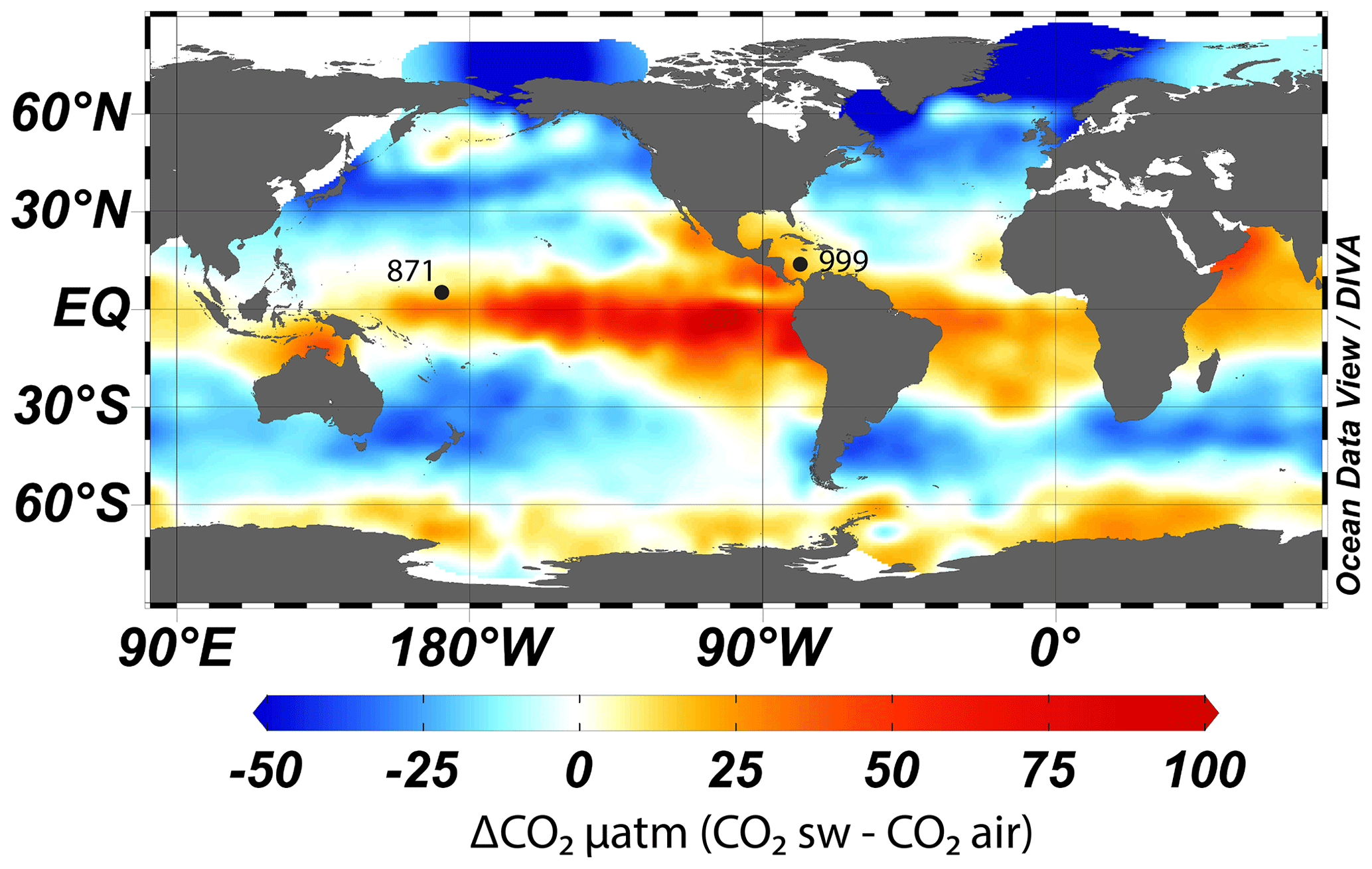
Figure 1Map of air–sea CO2 disequilibrium (seawater–air, in ppm) and location of ODP sites used in this study. CO2 data are from Takahashi et al. (2009). The map was made with Ocean Data View (Schlitzer, 2023).
While we recognise that both sites have a minor disequilibrium, this is often a necessary compromise as areas of the ocean that are in strict equilibrium with the atmosphere are often located in the middle of oceanic gyres and tend to have deep sediments located under the lysocline, have a low sedimentation rate, and/or are outside the preferred geographic habitat of G. ruber. Furthermore, we present surface δ18O and δ13C (site 871) and temperature (both sites) from G. ruber that provide insight into the potential influence of upwelling (see Sect. 4.2.2) at these locations. Recent Earth system model (IPSL-CM5A-MR) outputs (Gray and Evans, 2019) also show that relative pH difference at our core sites between the Last Glacial Maximum (LGM) and the pre-industrial period (PI) compared to the ocean average pH difference are close to 0, giving confidence that changes in local disequilibrium are unlikely to drive large changes in our CO2 reconstructions (at least during the last glacial period).
2.2 Samples
2.2.1 Sample selection and preparation
Samples of deep-sea sediment from our two study sites were taken at 6 cm (∼3 kyr) and 10 cm (∼6 kyr) resolution at ODP 871 and 999, respectively. Around 1–2 mg of the foraminifer (between 120 and 200 individuals) from the species Globigerinoides ruber sensu stricto white (hereafter G. ruber ss) were hand-picked from the size fraction 300–355 µm for a target of 10 to 20 ng of boron. G. ruber ss was chosen here because it is readily identified; is abundant throughout our chosen time interval; and a δ11Bforam-borate calibration that accounts for vital effects is available from culture, plankton tows, and core-top samples (Henehan et al., 2013). It is also known to live in the upper surface of the ocean with a relatively small depth range (Rebotim et al., 2017), which prevents significant influence of deeper, more remineralised CO2-rich waters on the measured δ11B. The morphotype G. ruber sensu lato (hereafter G. ruber sl) has slightly different morphology (Aurahs et al., 2011; Carter et al., 2017) and is thought to live in deeper water compared to G. ruber ss (Wang, 2000). The morphotype G. ruber sl was also hand separated and analysed at lower resolution at ODP 871 to monitor any change over time in morphotype differences in δ11B that could result from different habitats. For similar reasons, carbon and oxygen isotopes (δ18O and δ13C) were also measured on G. ruber ss and sl for comparison on the whole record at ODP 871. For this, around 10 individuals of G. ruber per sample were picked, their shells gently broken open and mixed and then a 100 µg aliquot of the homogenised carbonate was measured using a Thermo KIEL IV Carbonate device at the University of Southampton, Waterfront Campus. While this number of specimens is lower than classically done for δ18O and δ13C analysis, it provides power for the identification of species-specific preferential diagenetic alteration, which may have occurred in the sediment, and it was sometimes necessary due to the scarcity of some of the G. ruber spp. morphotypes.
2.2.2 Age constraints
Samples were taken from 1.5 to 5 m b.s.f. (metres below sea floor) for ODP 871 and from 9 to 21 m b.s.f. for ODP 999. Sample age at Site 871 was initially determined from sample depth using published age models (Dyez and Ravelo, 2013). At Site 999, the age was determined by developing a new Cibicidoides wuellerstorfi benthic δ18O record. The initial age model at Site 871 was refined by measuring δ18O on the benthic species Uvigerina peregrina (50 µg of 3–5 mixed, crushed, and homogenised specimens) measured on a Thermo KIEL IV Carbonate device at the University of Southampton, Waterfront Campus. These new δ18O data (Fig. 2) were then tuned to the benthic δ18O LR04 stack (Lisiecki and Raymo, 2005) using Analyseries (Paillard et al., 1996). A correction of +0.47 was applied to the δ18O Cibicidoides wuellerstorfi at ODP Site 999 following Marchitto et al. (2014).
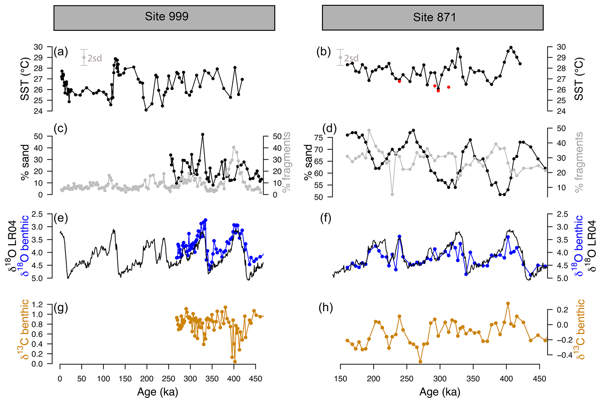
Figure 2-derived temperature, coarse fraction (sand), fragmentation, and benthic δ18O and δ13C at ODP sites 999 and 871. (a, b) Temperature at ODP 999 (from G. ruber ss, black, Schmidt et al., 2006, and this study) and ODP 871 (G. ruber ss, black, G. ruber sl, red, 2 SD indicated by the grey error bar). (c, d) Fragmentation index (light grey, data from Schmidt et al., 2006, for ODP 999) and sand (black line). (e, f) Benthic C. wuellerstorfi (Site 999) and U. peregrina (Site 871) δ18O (blue) and LR04 benthic δ18O stack (black). A correction of +0.47 ‰ is applied to δ18O of C. wuellerstorfi data to adjust for species offset. (g, h) Benthic C. wuellerstorfi (Site 999) and U. peregrina (Site 871) δ13C (orange).
2.2.3 Fragment counts
Foraminifera fragment counts were conducted on ODP Site 871 to monitor variations in carbonate preservation. Samples were sub-sampled using a splitter (in order to maintain homogeneity) and poured onto a picking tray. The fragmentation index (FI) was calculated following the approach of Howard and Prell (1994) and Berger (1970) where percentage fragment is defined as follows:
Counts of whole intact grains and fragments of grains were conducted three times and averaged. The standard deviation (1σ) of the fragmentation index is 1.69. This approach followed that used in an early study at ODP Site 999 (Schmidt et al., 2006), ensuring that the data sets between the two sites are comparable.
2.2.4 Boron separation
The hand-separated foraminifera tests for boron isotope analysis were broken open, detrital clay was removed, and oxidatively cleaned and leached in a weak acid to obtain a primary carbonate signal using established methods (Barker et al., 2003). Samples were then slowly dissolved in ∼100 µL 0.5M HNO3 added to 200 µL of MQ water. Dissolved samples were then centrifuged for 5 min to separate any remaining undissolved contaminants (e.g. silicate grains, pyrite crystals) and transferred to screw top 5 mL Teflon pots for subsequent boron separation. An aliquot equivalent to 7 % of each sample was kept for elemental analysis and transferred to acid-cleaned plastic vials in 130 µL 0.5M HNO3. Samples were purified for boron using anion exchange column chemistry method prior to isotope analysis as described elsewhere (Foster, 2008). A total procedure blank (TPB) was conducted for each batch of samples and typically ranged from 0 to 100 pg, which represents a blank contribution of up to 2.3 % (for samples containing ∼10–20 ng of boron). Most samples had a TPB below 40 pg and were not corrected. Two batches had a TPB of 70 and 100 pg, for which we corrected using a long-term median TPB δ11B value of −7.27 ‰ from the University of Southampton. This represents a δ11B correction of 0.1 ‰ to 0.7 ‰.
2.3 Analytical techniques
Boron isotope analyses were performed on a Thermo Scientific Neptune multi-collector inductively coupled plasma mass spectrometer (MC-ICPMS) with 1012Ω amplifier resistors using a standard-sample bracketing routine with NIST 951 boric acid standard (following Foster et al., 2013, and Foster, 2008). Elemental analysis was performed on each dissolved sample using a Thermo Scientific Element inductively coupled plasma mass spectrometer (ICPMS). All analyses were carried out at the University of Southampton, Waterfront Campus (following Foster, 2008, and Henehan et al., 2015). Element-to-calcium ratios were measured with 43Ca and 48Ca and measured against in house mixed element standards. Elemental ratios measured included , , , , and . Based on the reproducibility of our in-house standards, the uncertainty for most elemental ratios is ∼5 % (at 95 % confidence).
2.4 Constraints on δ11B-derived pH and CO2
2.4.1 From δ11B to pH
Seawater pH is related to the boron isotopic composition of dissolved borate ion by the following equation:
where the isotopic fractionation factor αB between B(OH)3 and B(OH) is 1.0272 as determined by Klochko et al. (2006) and the δ11B of seawater is 39.61 ‰ (Foster et al., 2010) for both sites and kept constant throughout the record due to the long residence time of boron (10–20 Myr, Lemarchand et al., 2002).
The sea surface temperature (SST) values necessary to calculate pKB in Eq. (5) were determined at both sites using the of G. ruber (Dyez and Ravelo, 2013) including a depth-dependent dissolution correction for each site (following Dyez and Ravelo, 2013, for Site 871 and Schmidt et al., 2006, for Site 999) and a pH correction using the iterative approach of Gray and Evans (2019) to account for the observed pH effect on in G. ruber producing higher apparent sensitivity of during glacial cycles (Gray et al., 2018).
was corrected for depth-dependent dissolution at Site 871 using the following equation (Dyez and Ravelo, 2013):
from Site 999 was corrected following Schmidt et al. (2006):
To evaluate the effect of various treatment on temperature and calculated CO2, we performed seven sensitivity tests (Table S1) with -derived SST using the calibrations of (1) Gray et al. (2018) temperature-dependent only (global calibration), (2) Gray and Evans (2019) with a pH correction, (3) Gray et al. (2018) temperature-dependent with corrected for depth-dependent dissolution, (4) Gray and Evans (2019) with corrected for depth-dependent dissolution and pH correction, (5) Anand et al. (2003) with and without a depth correction, and (6) with temperature kept constant (26 ∘C).
The differences in SST and resulting CO2 can be substantial (Fig. S1, Table S2): up to 6∘ and ∼50 ppm, respectively, between the Gray et al. (2018) calibration uncorrected for pH and the Anand et al. (2003) calibration corrected for dissolution. We have chosen the treatments that account for pH effect on and yield the closest agreement between coretop at both sites and modern temperature from Glodap v2 (Lauvset et al., 2022). This treatment is with a pH correction and corrected for depth-dependent dissolution. Choosing this approach is justified considering (1) the strong offset between Anand et al. (2003) multi-species –temperature calibration and the more recent G. ruber compilation of Gray et al. (2018), (2) the effect of pH correction as shown in Gray et al. (2018) and Gray and Evans (2019), (3) the suggested influence of dissolution on (Dyez and Ravelo, 2013; Schmidt et al., 2006), and (4) the better agreement between coretop and modern SST at each site when using a pH and depth correction (Fig. S1).
The salinity (S) that is used in the expression of pKB is kept constant for both sites (35) due to the very minor effect of salinity on calculated pH/CO2 (1 salinity unit changes pH by 0.006).
2.4.2 From pH to CO2
Calculating CO2 from boron-isotope-derived pH is dependent on the determination of a second parameter of the carbonate system. Here we use the modern value of total alkalinity (TA) at each site: 2279 and 2350 µmol kg−1 at ODP 871 and ODP 999, respectively (Shipboard Scientific Party, 1993; Takahashi et al., 2009). Following Chalk et al. (2017), these values were kept constant throughout the whole record. To account for any variations in alkalinity, a generous uniform (i.e. equal likelihood of values within the range of uncertainty) uncertainty of 175 µmol kg−1, distributed equally on either side of the central value, is applied. This range in TA encompasses the likely range in this variable on glacial–interglacial (e.g. Toggweiler, 1999; Hain et al., 2010; Cartapanis et al., 2018) or longer timescales (Hönisch et al., 2009), and its adoption means the local TA record is not tied to a global sea level record as has been practised previously. We avoid drawing this link because the % (+68 µmol kg−1) concentration increase in solute alkalinity occurring from sea level lowering during the Last Glacial Maximum may not have been the dominant driver of ocean alkalinity change (Boyle, 1988a, b; Sigman et al., 1998; Toggweiler, 1999; Hain et al., 2010; Cartapanis et al., 2018). By assuming a uniform distribution for TA, we avoid imposing a temporal evolution to this variable because evolution of TA through a glacial cycle is uncertain and is unlikely to be simply a function of sea level or salinity (e.g. Dyez et al., 2018) due to the effect of carbonate compensation.
The surface water CO2 is then calculated as follows (Zeebe and Wolf-Gladrow, 2001):
where TA is the total alkalinity, KB the equilibrium constant of boron species in seawater, BT the concentration of boron in seawater (432.6 µmol kg−1, Lee et al., 2010), [H+] the concentration of H+ determined from pH = −log[H+], KW the dissociation constant of water (function of T, S, and pressure), and K1 and K2 the first and second dissociation constants of carbonic acid (function of T, S, and pressure, Luecker et al., 2000). The estimate of atmospheric CO2 includes site-specific offsets relative to reconstructed surface water CO2 to account for observed local disequilibrium (+21 and +12 ppm at ODP Sites 999 and 871, respectively).
2.5 Uncertainty
2.5.1 Analytical uncertainty
The uncertainty of the measured δ11B is expressed as the external uncertainty, which includes instrumental error and chemical separation of the sample (see a detailed discussion in John and Adkins, 2010). This was determined empirically by long-term repeat measurements of JCp-1 subject to the same chemical purification as our foraminiferal samples. As discussed by Rae et al. (2011), this uncertainty is dependent on the intensity of the 11B signal and is expressed here by the following relationship defined during the duration of this study at the University of Southampton (Anagnostou et al., 2019) for 11B intensities < 0.54 V:
where [11B] is the intensity of 11B signal in volts. The δ11B uncertainty for 11B intensities > 0.54 V is 0.15 ‰ (at 95 % confidence).
2.5.2 The pH and CO2 uncertainty
The CO2 uncertainty we report was calculated with a Monte Carlo simulation (10 000 realisations) in order to fully account for the uncertainty in all variables used in the calculation of pH and CO2 (). The shape of the uncertainty distribution sampled is either normally distributed (for temperature, salinity, and δ11B) or uniform (for alkalinity, as discussed above). The maximum probability of all realisations was used as the central value for CO2, and an error envelope at 1 and 2σ was calculated based on the 68 % and 95 % distribution of the realisations.
2.5.3 Uncertainty of the CO2 offset
To constrain the offset between δ11B-derived CO2 and ice core CO2, each sediment age is compared to the ice core CO2 record by interpolation of the record of highest resolution (in this case the δ11B record onto the ice core compilation). To fully account for age uncertainty when interpolating the sediment age to the well-dated ice core record, a distribution of the ice core data was calculated within the 4σ uncertainty of the δ11B age and weighed by the respective likelihood based on the age difference between ice core and sediment core (Hain et al., 2018).
The CO2 offset (or residual) is defined by the following equation:
The uncertainty of this offset (σoffset) accounts for the uncertainty of the interpolated ice core CO2 () and the one of the δ11B-derived CO2 (), such as the following equation:
2.6 The relationship between δ11B-derived pH and ΔF
The linear relationships between the relative CO2 forcing ΔF and pH are determined with a York regression (York et al., 2004) that accounts for the uncertainty in both the independent and dependent variable (i.e. x and y axes). The ice core CO2 interpolation used to calculate ΔF and uncertainty is determined as described in Sect. 2.6.3 (Hain et al., 2018).
2.7 Optimising the G. ruber δ11B borate-foraminifera calibration
An optimised G. ruber calibration was obtained by minimising the root-mean-square error (RMSE) of the average offset between δ11B-derived CO2 and ice core CO2. The steps are illustrated in Fig. S2. In order to optimise the calibration, 10 000 simulations of δ11Bborate and δ11Bforaminifera from the calibration of Henehan et al. (2013) were performed within their normally distributed uncertainty (1σ), from which we defined the same number of linear models each including their slope and intercept. We then calculate the equilibrium pH and resultant equilibrium δ11Bborate from ice core CO2 and the assumed constant TA at each core site. The δ11Bborate from the 10 000 linear models is then calculated, and the difference from the ice core-derived δ11Bborate is determined. The linear model calibration that yields the minimum RMSE between these two borate variables defines the new δ11Bforam–borate calibration. To assess the effect of δ11B records from different sites, we performed this exercise using the combined records (from both sites 999 and 871), 999 only, and 871 only (Fig. S3) and show that using a record from one particular site or the combination of sites yields similar CO2 offsets (Table S3), and thus here we use the results from the combined sites. Unless indicated otherwise, to preserve a degree of independence, the pH results presented in this study are calculated with the published calibration (Henehan et al., 2013), and the results with the optimised calibration are presented in Sect. 4.2.6.
3.1 Temperature and fragment counts
The SST at ODP Sites 999 and 871 show a cyclicity that agrees with the well-known glacial–interglacial cycles of the late Pleistocene (Fig. 2). The SST determined from G. ruber sl (filled red circles, Fig. 2b) at Site 871, show equal or cooler temperatures (by 1–2 ∘C) than G. ruber ss (filled black circles). The fragmentation index (Fig. 2d) at ODP 871 ranges from 20 % to 50 % and follows the well-documented “Pacific style” dissolution cycles (Sexton and Barker, 2012) with well-preserved carbonate (low fragments) during glacials and less well-preserved carbonates (higher fragments) during interglacials. The percentage sand typically anti-correlates with fragmentation counts at both sites, although it is less clear at ODP 999, perhaps due to the shorter record available. Fragmentation counts reach maxima at ODP 999 of 20 % during interglacials and up to 50 % during marine isotope stage (MIS) 11 at 400 ka, which is concomitant with the Mid-Brunhes Dissolution Interval (MBDI, Barker et al., 2006). The fragmentation counts at ODP 871 show no substantive anomaly during the MBDI.
3.2 The pH and CO2 reconstructions
The δ11B, pH, and δ11B-derived absolute CO2 (Fig. 3) from Sites 871 and 999 show clear cyclicity related to glacial–interglacial cycles. The CO2 values carry an average uncertainty of ±48 ppm, and the mean offset from the ice core CO2 for a combination of the two records is 13±46 (2σ) ppm, showing that there is a minor overestimation of CO2 using the boron method, but it agrees well on average within uncertainty. The RMSE of the CO2 offset for the combined record is 26 ppm.
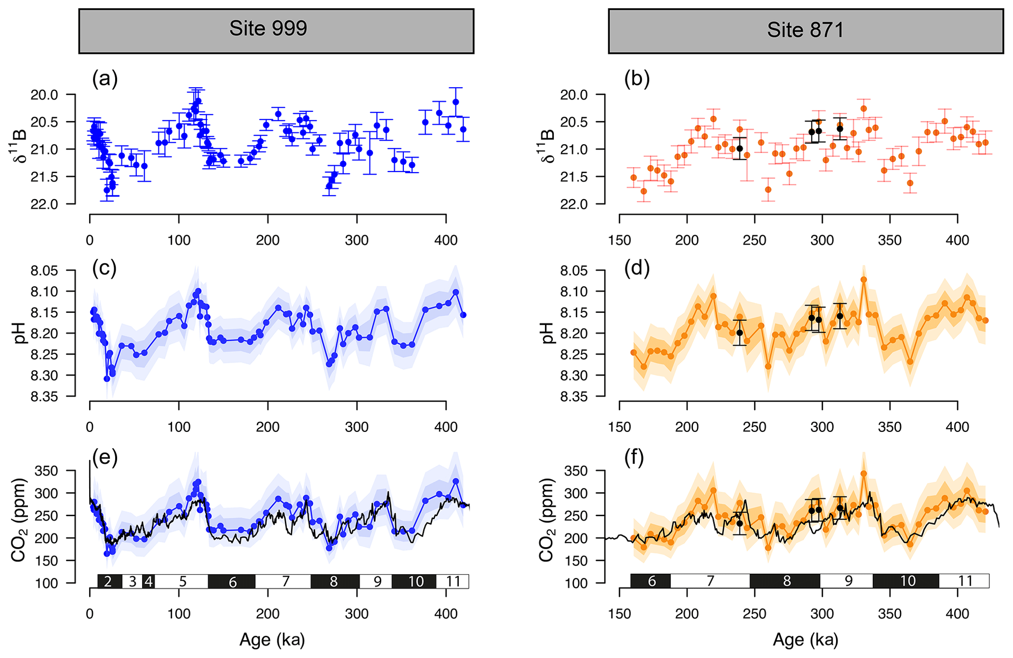
Figure 3The δ11B, pH, and boron-derived CO2 at site 999 and 871. The δ11B of G. ruber ss and sl (a, b), boron-derived pH (c, d), and CO2 (e, f) reconstruction from two core locations: ODP 999 (blue, this study and published data, Foster, 2008; Henehan et al., 2013; Chalk et al., 2017) and ODP 871 (orange, this study). The black line in the CO2 panels is the composite Antarctic ice core CO2 record (Bereiter et al., 2015). All δ11B-derived data points are from G. ruber ss except the black dots at ODP Site 871 measured on G. ruber sl. Numbers at the bottom of the CO2 records represent marine isotope stages (black boxes for glacials and white boxes for interglacials). Note the age scale is different between Sites 999 and 871.
Despite the overall close agreement between δ11B-derived CO2 and ice-core-derived CO2, each of our δ11B–CO2 records exhibit some short-lived intervals where the offsets from the ice core record are larger. This is further revealed by the residual CO2 and the identification of the data above the upper quartile (i.e. the upper 25 % of the data, Fig. S4). Those data do not appear to be randomly distributed and instead occur at ∼100, ∼220–290, and ∼390 ka at ODP Site 999, in all three cases during the early stages of the glaciation (except for the MIS 8 glacial at 280 ka, Fig. S4). The mismatches with the ice core at ODP Site 871 show a similar temporal pattern occurring at ∼220 and ∼300 and ∼350–390 ka (i.e. at glacial inceptions).
3.3 Contrasting δ11B between morphotypes
Within error, the few measurements of δ11B G. ruber sl at ODP 871 all agree with δ11B G. ruber ss (Fig. 3), although the δ11B data of G. ruber sl are higher than G. ruber ss for all four data pairs available. The CO2 derived from G. ruber sl (Fig. 3) is on average 22 ppm lower than the one derived from G. ruber ss; though the much lower resolution (n=4) impedes a thorough comparison at this stage. The δ18O and δ13C of both morphotypes were compared for the whole records at ODP 871 (Fig. S5), and a cross-plot shows a moderate to good agreement between G. ruber ss and G. ruber sl (r2=0.55 and 0.22 for δ18O and δ13C, respectively, Fig. S6). This is in contrast to other studies (e.g. Wang, 2000; Steinke et al., 2005) that show δ18O in G. ruber sl to be systematically higher.
3.4 Relationship between δ11B-derived pH and CO2 forcing from the ice core
A cross plot of δ11B-derived pH CO2 forcing from the ice core record for each of our marine core study sites is shown in Fig. 4 and is compared to the theoretically derived approximate ΔFpH relationships as adopted by Hain et al. (2018): W m−2 (dashed black line), CaCO3 addition or removal ( W m−2 plain yellow line), DIC addition or removal ( W m−2 dashed–dotted blue line), and warming or cooling temperature forcing ( W m−2, dashed red line). Our analysis includes full propagation of uncertainty in pH, in contrast to Hain et al. (2018), who considered only the reported uncertainty of δ11Bborate in their validation exercise. In both cases the uncertainty in ΔF accounts for the error in interpolation arising when comparing age-uncertain δ11B-derived pH with ΔF from the well-dated and high-resolution ice core CO2 record (see Sects. 2.7 and 2.6 for details). This treatment of ΔF uncertainty is dominated by the spread of ice core CO2 data points within the δ11B age uncertainty. The data are fitted with a York-type regression (thin black line; York et al., 2004) where the grey envelope represents the uncertainty of the linear relationship that best represents the data (i.e. the envelope is not the prediction interval), considering the uncertainty in pH and ΔF. The regressed slope is ΔFpH = W m−2 ( relative to basic formalism) and shows a good agreement with the theoretical temperature- and DIC-driven relationships.
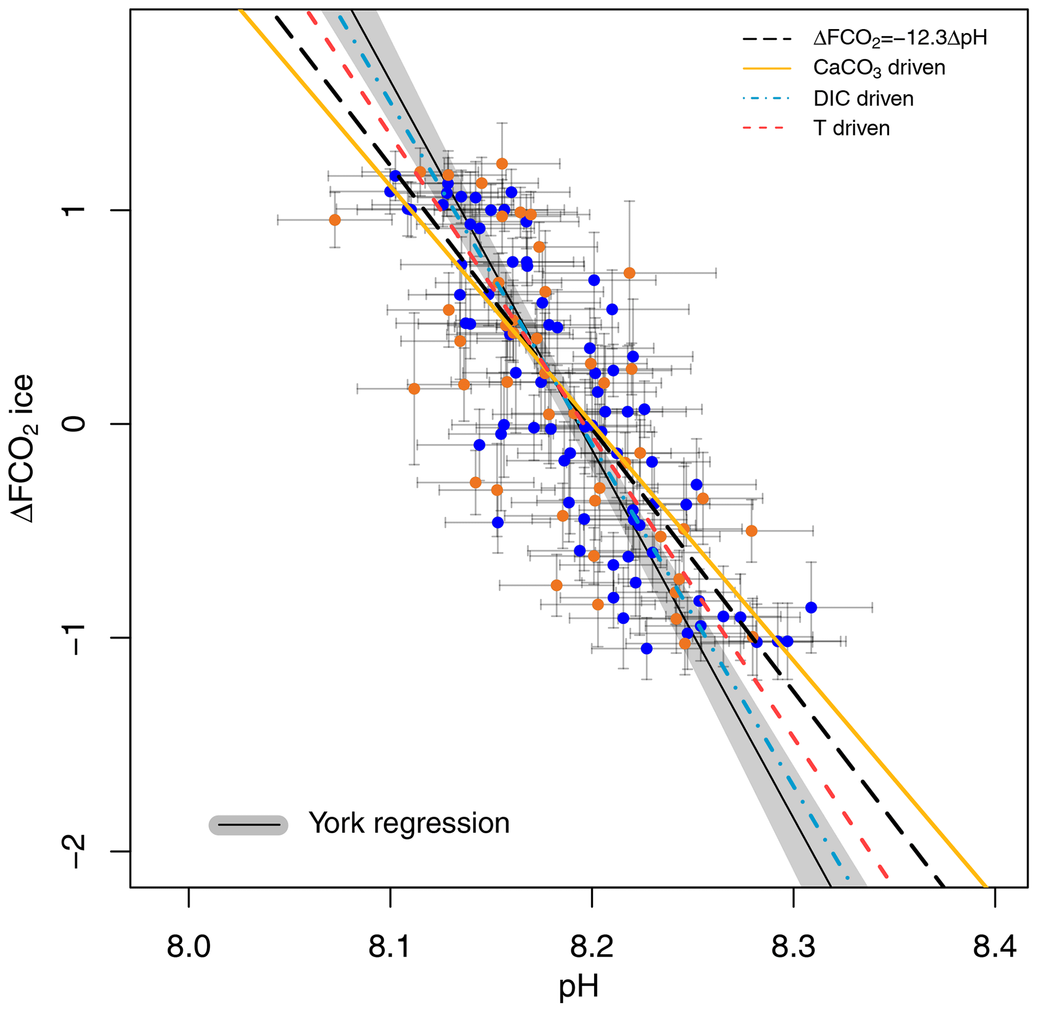
Figure 4Ice-core-based ΔFCO2 (CO2 forcing) vs. δ11B-based pH for ODP 999 (filled blue circles, this study and published data from Foster, 2008; Henehan et al., 2013; Chalk et al., 2017) and 871 (filled orange circles). The lines show the relationship between ΔFCO2 and pH for the simplified formalism (see Sect. 2) ΔFCO ΔpH (dashed black line) and when driven by changes in DIC only (dashed–dotted blue line, ΔFpH = −16 W m−2), CaCO3 (yellow line, ΔFpH = −11.1 W m−2), and temperature T (dashed red , ΔFpH = −14.1 W m−2). The York regressed line (thin black line and grey shading) falls close to the DIC-driven line (dashed–dotted blue line).
The effect of the uncertainty assigned to pH (fully propagated or using the measurement uncertainty of the boron isotope) on the regressed slope is shown in Fig. S7. The slope of the York regression when using the uncertainty from δ11B only, as in Hain et al. (2018), shows a close agreement with the basic formalism, with a slope of ΔFpH = W m−2, ( relative to the basic formalism) but with a unsatisfactory goodness of fit (mean squared weighted deviation, MSWD) of 5.3, whereas propagating the full pH uncertainty based on our iterative Monte Carlo simulations improves goodness of fit to ∼0.9 at a Δlog 10COpH of (Fig. 4).
4.1 Cyclicity in foraminifera preservation
Percentage fragments and sand fraction (>63 µm) at both studied core sites are anticorrelated and show a clear cyclicity, with better preservation of carbonates during glacial periods (Fig. 2). The anticorrelation is clearer at ODP Site 871, where we have the longest record (Fig. 2). Preservation in the Pacific (Farrell and Prell, 1989) shows improved (poorer) preservation during glacial (interglacial), and this pattern seems to have originated after the Mid-Pleistocene Transition (Sexton and Barker, 2012). The origin of these cycles could be a combination of enhanced ventilation during glacials in the Pacific (Sexton and Barker, 2012) or increased burial due to enhanced global alkalinity following a decrease in burial in the Atlantic (Cartapanis et al., 2018). However, glacial periods seem to have been accompanied by a diminution in oxygenation in the deep Pacific (Anderson et al., 2019) that may have also impacted preservation.
The observation that the fragmentation records of sites 999 and 871 covary is likely attributable to the different water masses that fill the Caribbean basin relative to the rest of the Atlantic basin. During glacials, the deep Atlantic is filled by nutrient- and carbon-rich corrosive southern-sourced waters (Antarctic Bottom Water) with a reduced contribution from the less corrosive, nutrient-poor North Atlantic Deep Water (Oppo and Lehman, 1993) causing calcareous sediments in the deep Atlantic Ocean > 2500 m to be less well preserved during glacials than interglacials. The opposite pattern of dissolution is seen in the Caribbean because shoaling of the northern-sourced waters during glacials produces a mid-depth well-ventilated water mass that feeds into the Caribbean through its deepest sill (∼1900 m, Johns et al., 2002). Thus, the deep Caribbean is filled with less corrosive waters during glacials than interglacials, improving the preservation of carbonate during glacials in a similar pattern to a Pacific-styled dissolution cycle, albeit in response to Atlantic circulation changes. During interglacials, the northern-sourced waters are mixed with corrosive southern-sourced waters (Antarctic Intermediate Water and Upper Circumpolar Deep Water), leading to sediments that less well preserved.
4.2 Causes of offset between δ11B-derived and ice core CO2
The δ11B-derived CO2 record from both of our study sites is in very good agreement with the ice core record, with an average offset for combined both cores of 13±46 (2σ) ppm and corresponding RMSE of 26 ppm. However, the minor CO2 offsets observed in both records do not appear to be random and tend to fall during the first half of each glacial cycle (Fig. S4). In order to have the highest confidence in CO2 reconstructions using δ11B, this pattern warrants further investigation (see below).
4.2.1 Comparison between morphotypes of G. ruber
If, as others suggested (e.g. Wang, 2000; Steinke et al., 2005; Numberger et al., 2009), G. ruber sl and G. ruber ss occupied different depth habitats, then inadvertent sampling of the cryptic G. ruber sl morphotype might conceivably produce the biases we observe between δ11B-derived CO2 and atmospheric CO2 from the ice cores. However, while our -derived temperatures for G. ruber sl and G. ruber ss display variable offsets, they are within uncertainty (Fig. 2) and our δ18O and δ13C data for the two morphotypes at ODP 871 show a good agreement with no consistent differences (Fig. S5). Thus, while the water column profile of δ18O and δ13C can be affected by factors other than temperature, salinity, and biological productivity (e.g, carbonate ion effect, Spero et al., 1997), our data overall suggest that the two morphotypes we analysed shared similar depth habitat preferences.
Henehan et al. (2013) found that G. ruber ss and G. ruber sl record similar δ11B in core-top sediments and through necessity used mixed morphotypes in their culture study. The δ11B-derived pH and CO2 for G. ruber sl examined here are consistently higher and lower than G. ruber ss by around +0.02 pH units and −22 ppm CO2 on average, respectively (Fig. 3). This is contrary to expectation if G. ruber sl lived in deeper and more acidic waters as suggested by other studies (Wang, 2000; Steinke et al., 2005) but consistent with some data sets that show that the habitat of G. ruber ss and G. ruber sl can vary by location and seems to be dependent on local productivity (Numberger et al., 2009). Other data sets from the Atlantic and Indian oceans nevertheless show similar between both morphotypes (Gray et al., 2018). We acknowledge that the scarcity of G. ruber sl in our samples means that our data set for this morphotype is too small to draw firm conclusions, and this warrants further investigation at other study sites. Nonetheless, the closeness of the morphotypes in terms of δ11B and depth habitat throughout our record implies any inadvertent sampling of G. ruber sl in the G. ruber ss fraction in this study and location would not significantly bias our reconstructions.
4.2.2 Change in upwelling and CO2 disequilibrium
ODP sites 871 and 999 are today both located in stratified oligotrophic environments with a deep modern thermocline (the base of the thermocline is at ∼200 and 400 m at ODP 871 and 999, respectively; Olsen et al., 2016). It should be noted, however, that both sites are situated relatively close to regions displaying ΔpCO2>40 ppm (Fig 1). However, if local upwelling occurred over the study interval or if these areas of upwelled water expanded, we would expect these periods to be characterised by relatively low SST, high surface δ18O, and low surface δ13C due to an increased influence of colder and more remineralised deep waters. The identified anomalous intervals in residual CO2 at ODP 871 (e.g. at ∼210, ∼290 ka, Fig. 5) show no particular anomaly in planktonic C and O isotopes (Fig. S5) or in SST (Figs. 2 and S8), ruling out significant variations in upwelling at that site. The -derived SST record of nearby Site MD97-2140 (Fig. S8) from the Western Pacific Warm Pool (de Garidel-Thoron et al., 2005), a location outside of the upwelling from the Pacific cold tongue, confirms this view in that the periods of high CO2 offset at Site 871 are not associated with relatively cold periods at site MD97-2140. Equally, no SST anomaly was identified at ODP 999 to be coincident with the intervals of high residual CO2. Foster and Sexton (2014) have also reconstructed CO2 zonally across the equatorial Atlantic and the Caribbean and showed that while enhanced disequilibrium was detected in the eastern Atlantic, Site 999 has remained in equilibrium with the atmosphere for the last 30 kyr at least. This suggests the CO2 anomalies revealed in Fig. 5 are not the result of enhanced local disequilibrium via sub-surface water mixing. Whilst SST is a first-order constraint on upwelling, we acknowledge future constraints are needed using paired proxies of local CO2, temperature, and productivity to evaluate changes in local CO2 fluxes.
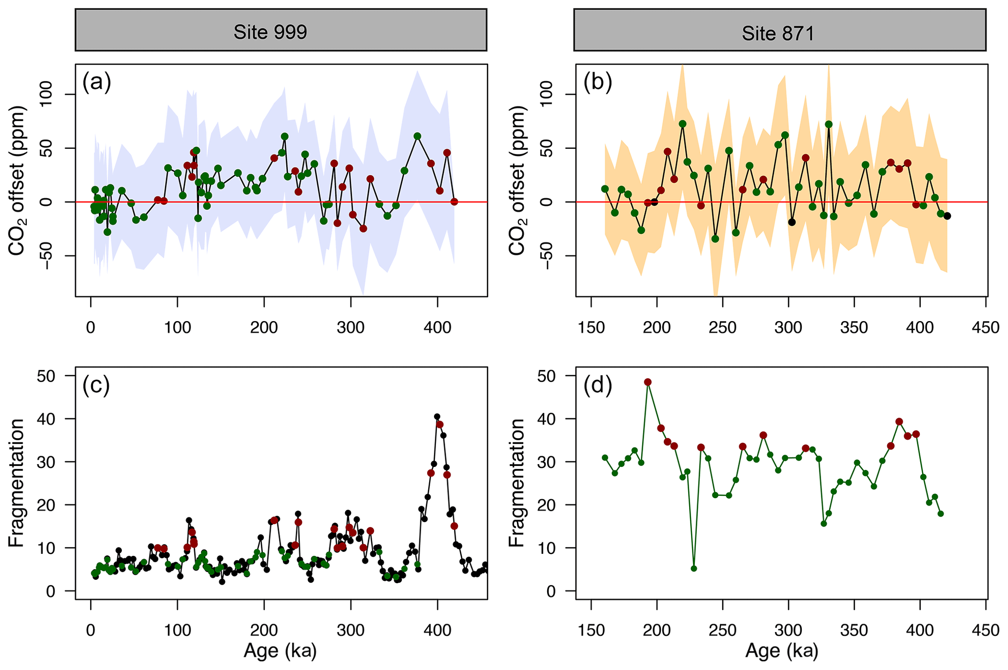
Figure 5(a, b) CO2 offset (defined as offset being equal to CO2_δ_11B-derived–CO2_ice) for ODP Sites 999 (this study and Chalk et al., 2017) and 871. See the text for error bar calculations. (c, d) Fragmentation index at Site 999 (Schmidt et al., 2006) and 871 (this study). Red dots in (c, d) are the fragments above the upper quartile (and corresponding CO2 in a, b, red dots). Green dots represent periods of low fragments below the upper quartile (and corresponding CO2 in a, b, green dots).
4.2.3 Partial dissolution
The CO2 derived from G. ruber δ11B at ODP 999 and 871 appears to show, at the first order at least, positive CO2 offset during periods of high fragmentation (∼100, ∼210, ∼400 ka, filled red circles in Fig. 5, defined by the upper 25 % quantile of fragments) following a “Pacific style” dissolution cycle (better preservation and lower fragmentation during glacial periods). Periods of high fragmentation at ODP Site 999 and 871 correspond to a positive CO2 offset 65 % and 75 % of the time, respectively, and 35 % and 25 % of the time to a negative or no (i.e. ±10 ppm) CO2 offset (note that values ± 10 ppm were omitted in the criteria for positive or negative offset). We also note that almost all CO2 offset uncertainties (2σ) overlap with the 0 line; hence, the percentage of CO2 offsets that are above or below the 0 line should be interpreted with caution.
In detail, however, a cross-plot of fragment counts and CO2 offset (Fig. S9) fitted with a linear regression shows no significant correlation for both core site 999 (r2=0.06, p=0.03) and 871 (r2=0.002, p=0.77). Although it should be noted that this simple linear regression presupposes a linear relationship between the variables and does not account for the significant uncertainty in both CO2 offset and fragmentation index. In particular, the CO2 offset carries the uncertainty from the interpolated ice core CO2 (see Sect. 2). Fragment counts at ODP 999 also come with the additional uncertainty related to the interpolation of the record of Schmidt et al. (2006), whereas fragments counts and δ11B-derived CO2 at 871 are measured on the same samples. A cross-correlation function also shows no correlation between CO2 offset and fragmentation (Fig. S10).
While it seems unlikely the small offsets observed are fully explained by partial dissolution, the positive CO2 offsets observed during some periods of high fragmentation index (Fig. 5) are in line with trends observed in other species like T. sacculifer (sacc). For instance, field studies observed lower δ11B in T. sacculifer for core-top samples from deeper ocean sites bathed by waters with a low calcite saturation state (Hönisch and Hemming, 2004; Seki et al., 2010). Tests of T. sacculifer can contain a significant proportion of gametogenic calcite (ranging 30 % to 75 % of the weight of pregametogenic calcite, Bé, 1980; Caron et al., 1990), which forms at the end of the life cycle in deeper lower pH cold waters. It has been suggested that δ11B is lower in gametogenic calcite than in the primary test (Ni et al., 2007), reflecting the digestion and expulsion of symbionts (Bé et al., 1983) before gametogenesis and driving a relative acidification of the micro-environment (no CO2 uptake by photosynthesis) around the foraminifera (Zeebe et al., 2003; Hönisch et al., 2003; Henehan et al., 2016) and movement to deeper more acidic waters during that life stage. It has been shown that this gametogenic calcite is more resistant to dissolution (Hemleben et al., 1989; Wycech et al., 2018), resulting in partial dissolution acting preferentially on ontogenic calcite and driving δ11B in the residual test to lower isotopic composition.
However, while the decrease in δ11B in tests of T. sacculifer found in corrosive waters is well explained by the lighter isotopic composition of gametogenic calcite, G. ruber tests do not contain such gametogenic calcite (Caron et al., 1990). Hence, if the observed occasional decrease in δ11B (low pH, high CO2) was caused by partial dissolution, it needs to be explained by other processes. It should also be considered that alternative measures and proxies of dissolution (e.g. benthic as an indicator of bottom water carbonate ion concentration) may yield more quantitative constraints on the importance of dissolution in generating our observed CO2 offsets. Some studies have shown that laboratory-dissolved specimens of T. sacculifer (Sadekov et al., 2010) and naturally dissolved specimens of G. ruber (Iwasaki et al., 2019) undergo targeted partial preferential dissolution of the shell. However, variations in intra-shell δ11B are currently unknown due to limitations in laser ablation techniques that currently impede a direct evaluation of δ11B heterogeneity in foraminifera chambers. Future studies are needed to constrain the δ11B spatial distribution in foraminiferal shells caused by potential variations in δ11B from dissolution, ontogeny (e.g. Meilland et al., 2021), and/or vital effects (e.g. change in photosymbiotic activity throughout the life cycle, Lombard et al., 2009; Henehan et al., 2013; Takagi et al., 2019). In the absence of these constraints, we conclude that partial dissolution is unlikely to be a significant driver of the δ11B–CO2 records we present here. Even though it was thought to be a species susceptible to dissolution (Berger, 1970), we confirm that the δ11B of G. ruber appears more resistant to dissolution-driven modification than T. sacculifer.
4.2.4 Effect of dissolution on and calculated CO2
The direction of change in with partial dissolution is towards lower ratios in partially dissolved foraminifera (e.g. Brown and Elderfield, 1996; Dekens et al., 2002; Fehrenbacher and Martin, 2014). If the is impacted during periods of high fragmentation, the lower ratio would result in lower temperatures, leading to lower calculated CO2 values (Eq. 7). This effect is opposite to the occasional positive deviation of CO2 observed during intervals of high fragmentation at ODP Site 999. While the weak correlation between fragmentation and CO2 precludes a firm interpretation of dissolution effect, we conclude that the effect of partial dissolution on ratio and resulting CO2 (if any) are negligible and not responsible for the CO2 offsets observed during intervals of high fragmentation.
4.2.5 Change in the second carbonate parameter: alkalinity
Past changes in TA are poorly constrained, although some constraints are starting to emerge for the late Quaternary (e.g. Cartapanis et al., 2018). However, since pH is directly determined by δ11B, pH defines the ratio of alkalinity to DIC (see Sect. S11). Hence, at any given pH, any change in alkalinity must be counteracted by a change in DIC, which has the opposing effect on CO2. This is demonstrated by the tight relation between pH and CO2 highlighted by our data (Fig. 4). The largest residual CO2 is ∼50 ppm at ODP 999. To produce an effective alkalinity-driven change in CO2 of this magnitude at a given pH requires an alkalinity reduction of about ∼300 to 500 µmol mol−1 (Fig. S12). This is far larger than any expected change over a glacial cycle (Cartapanis et al., 2018; Hönisch et al., 2009). We therefore rule out varying TA as the cause of the minor CO2 offsets observed (Fig. 5).
4.2.6 Improving the δ11B-pH G. ruber calibration
A further potential cause for the minor offsets observed between δ11B-derived and ice core CO2 could be a small inaccuracy in the calibration between δ11B of foraminifera and borate for G. ruber (Henehan et al., 2013). Having the ice core data to compare with δ11B-derived CO2 offers an opportunity to explore the effect of altering the input variables of the pH-CO2 calculation to see if doing so improves the fit to ice core values. Note that such an exercise is for illustrative purposes only because we seek to retain the independence offered by the δ11B-calibrated data in the context of CO2 forcing (Sect. 4.3). Nonetheless, in future work we suggest this calibration can be applied in tandem to the empirical relationship of Henehan et al. (2013). The published (Henehan et al., 2013) and obtained optimised calibration (Fig. S13) are as follows:
The newly calculated CO2 with the updated calibration shows an improved average CO2 offset (Fig. 6) of ppm (vs. 13±46 (2σ) ppm with the calibration of Henehan et al., 2013) and an RMSE of 18 ppm (vs. 26 ppm with the published calibration).
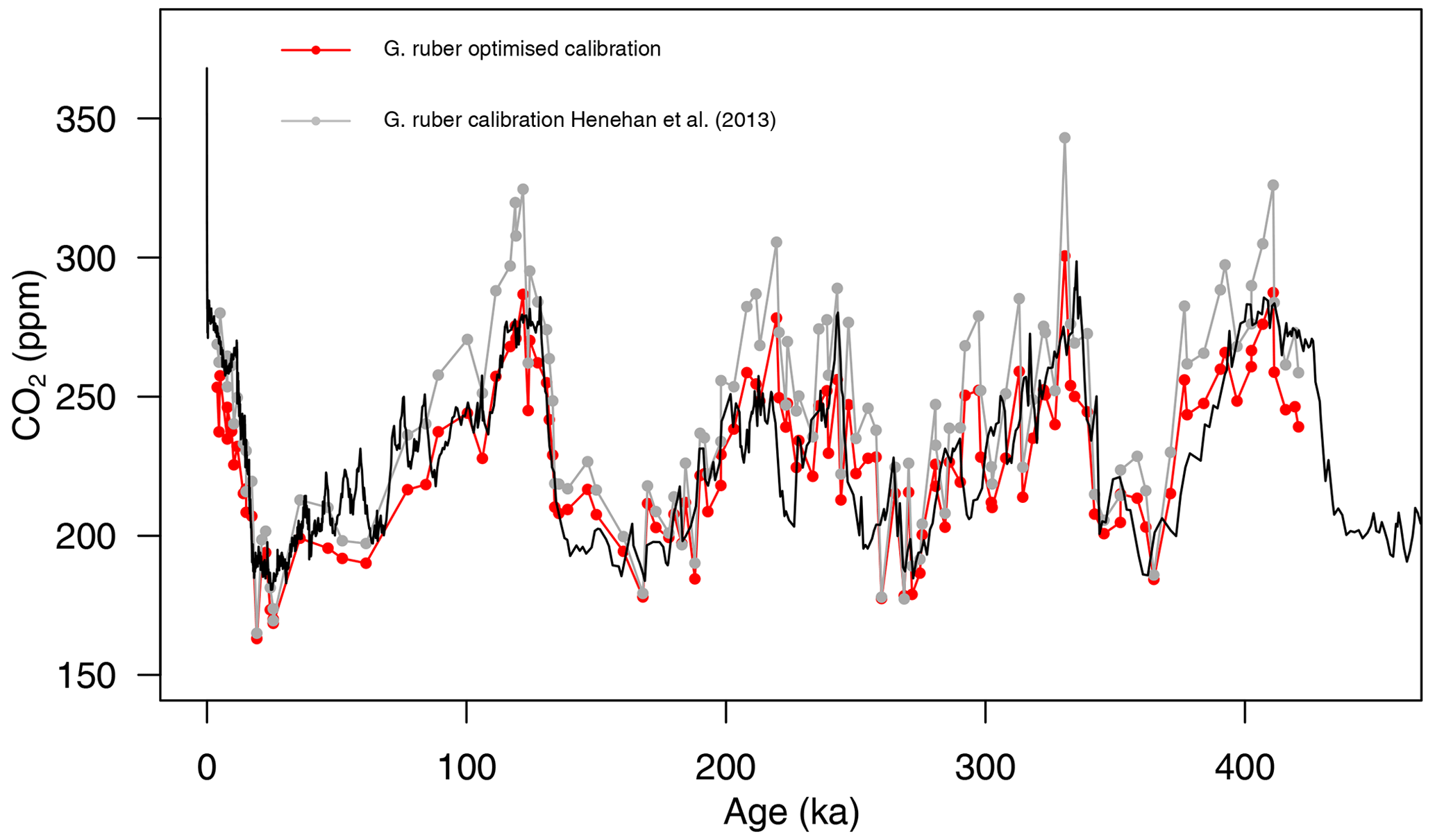
Figure 6Composite δ11B-derived CO2 from both core sites 999 and 871 using the published δ11Bforam–borate calibration (grey points, Henehan et al., 2013) and the optimised calibration (red points). The black line is the Antarctic composite ice core CO2 record (Bereiter et al., 2015).
When analysing the CO2 offset using the optimised G. ruber calibration and the fragmentation index at each core location (the same approach as Fig. 5), we observe that intervals of high fragments (defined as values above the upper quartile) are no longer preferentially associated with positive CO2 offset (Fig. S14). Intervals of high fragments occur 5 % and 33 % of the time at Site 999 and Site 871, respectively, during positive CO2 offsets (and 95 % and 67 % of the time during negative or no offset to the ice cores, respectively).
This analysis shows that a small change in the borate G. ruber δ11B calibration is enough to improve the fit to the ice core and diminishes the apparent correlation between high fragmentation and CO2 offset (Fig. S14) and that uncertainty in the δ11Bforam-borate calibration of Henehan et al. (2013) can – at least partly – explain the minor discrepancies we observe between δ11B-derived and ice core CO2.
4.3 Relative CO2 forcing and pH
Our new pH data, added to the existing compilation, show a good agreement with the formalism defined by Hain et al. (2018; Fig. 4). It should be noted that CO2 in this case is provided by the ice core directly and is not estimated from the δ11B-derived pH. As discussed above, because these two proxies are independent of one another, the slope of their relationship may be used to interrogate the mechanisms of CO2 change. Our data fall between the CaCO3 (plain yellow line) and the DIC (dotted-dashed blue line) end-members, suggesting that the CO2 change observed on glacial–interglacial timescales was driven by a mix of mechanisms rather than a single cause. This is in line with studies that require a number of mechanisms to explain glacial–interglacial CO2 change such as the soft tissue pump, carbonate compensation pump, solubility pump (e.g. Brovkin et al., 2007; Kohfeld and Ridgwell, 2009; Hain et al., 2010; Chalk et al., 2019; Sigman et al., 2021), and disequilibrium pump (Eggleston and Galbraith, 2018). We note that this is a preliminary interpretation because of the sensitivity of our finding to pH uncertainty (Sect. 3.4, Fig. S7). To overcome this ambiguity in estimating past ΔF and to better deconvolve the driving mechanisms of glacial–interglacial CO2 change, we recommend that future studies collect pH data at higher temporal resolution to examine the change in slope through a glacial cycle and strive to further quantify and reduce uncertainties related to pH determination.
The close agreement of the pH and ice core CO2 data with the theoretical relationships has a number of consequences for the reconstruction of CO2 change during periods of Earth's history beyond the ice core CO2 and climate records where constraints on δ11Bsw and the second carbonate parameter and temperature are uncertain. The ΔpH formalism still requires an estimation of δ11Bsw and temperature (for the pKB term, Eq. 5); however, as discussed in Hain et al. (2018), while absolute reconstruction of pH is significantly influenced by estimates of δ11Bsw and temperature, reconstruction of relative pH change (ΔpH) is inherently much less sensitive to these input variables.
Reconstructing ΔF from ΔpH is ideally applicable only on relatively short timescales less than 1 Myr, when δ11Bsw is likely to be invariant given the multi-million-year residence time of boron in the ocean (Lemarchand et al., 2002; Greenop et al., 2017). Furthermore, to reconstruct ΔF (and thus climate sensitivity to CO2), the formalism can be applied as long as ΔpH remains the overwhelming control in Eq. (2). This is dependent on the residence time of carbon in the ocean with respect to silicate weathering – approximately a million years (Hain et al., 2018), such that net carbon addition to or removal from the Earth system through volcanic outgassing or silicate weathering is likely to be minor over the million-year timescale. However, during some short events, for instance the Paleocene–Eocene Thermal Maximum, considerable carbon was added to the system in <200 kyr (e.g. Gutjahr et al., 2017), invalidating the formulation described in Eq. (2) on these intervals. We also emphasise that this formalism is only valid as long as core sites remain in equilibrium with the atmosphere.
4.4 Caveats and future studies
The aim of this study is to evaluate the capacity of the δ11B–pH proxy in G. ruber to accurately reconstruct atmospheric CO2 in the past. The overall agreement with the high-confidence ice core CO2 (e.g. Bereiter et al., 2015) is very promising and gives confidence to δ11B-derived CO2 reconstructions beyond the ice core record (>800 ka). We have, however, identified occasional minor offsets between the two records and explored potential drivers (partial dissolution, δ11Bforam–borate calibration, local air–sea disequilibrium). It is likely that the minor disagreement observed (Fig. 5) has a combination of drivers and that a single mechanism is not solely responsible for the CO2 offsets observed. To confirm these trends, we recommend future work to focus on the following points.
-
The improved δ11B calibration approach should be tested at more core locations. We note that the improved calibration to the ice core records reported here was achieved using data from two sites. While care is taken in the choice of study site to minimise air–sea CO2 disequilibrium and sediment dissolution, the newly defined improved δ11Bforam–borate calibration should be seen as an exercise that is tailored to the available data in this study, and future high-resolution studies can apply the method used here (Sect. 4.2.6) to further test how the G. ruber calibration changes if CO2 offsets occur in a similar fashion (i.e. at a particular time in each glacial cycles). We note the importance of high-resolution (at least 3 kyr) sampling in future studies because most CO2 offsets observed are short lived.
-
A multiproxy approach is ideally needed. In particular, reliable indicators of temperature and productivity are needed to assess change in upwelling and foraminifera ecology. We encourage future studies to expand high-resolution boron-derived CO2 record and ancillary data (C and O isotopes, proxy of carbonate preservation and bottom water corrosiveness, biological productivity) to further constrain the capacity of the boron isotope pH/CO2 proxy to generate reliable CO2 records. As more recent IODP expeditions include porewater data, constraints on bottom water conditions and the degree of corrosiveness at a given site will become available to evaluate the impact on δ11B signals in foraminifera.
-
Efforts should continue to decrease the analytical uncertainty associated with a δ11B measurement by MC-ICPMS because this still accounts for ∼40 % of the total uncertainty associated with each δ11B-derived CO2 estimate.
-
We find little evidence to suggest that partial dissolution of foraminiferal tests (G. ruber) is a major driver of uncertainty in δ11B-derived CO2 estimates, but well-constrained dissolution experiments are desirable because of site-to-site differences in foraminifera taphonomy.
We carried out the most thorough test to date of the δ11B–pH (CO2) proxy by comparing new high-resolution (3 to 6 kyr per sample) boron-isotope-based pH and CO2 at two locations with CO2 from the ice core record. Results suggest that the boron isotope proxy is robust and suited to reconstructing CO2 to a precision of ±46 ppm (2σ, RMSE = 26 ppm) over this interval, with little or no systematic bias shown by a mean residual of 13±46 (2σ) ppm. This provides high confidence to the application of the proxy beyond the reach of the ice core records.
Despite the overall good agreement, there are some minor short-lived CO2 offsets that appear to have some temporal structure and we explored a number of possible drivers. A visual correlation between CO2 offset and fragmentation index at core site 999 is observed (Fig. 5) but is not statistically significant. The effect of partial dissolution on δ11B in G. ruber appears to be negligible in our record, but the possible heterogeneity of δ11B within shells and variable susceptibly to dissolution of the different parts of the foraminifera encourage further exploration.
A revised δ11B borate–foram calibration was calculated by minimising the offset between δ11B-derived CO2 and ice core CO2 using published calibrations (Henehan et al., 2013). While the new calibration improves the fit to the ice core records, we caution against its use to estimate CO2 given that it is no longer independent of the ice core or the assumptions we make here to calculate CO2 (i.e. that TA is constant).
The formalism established by Hain et al. (2018) is robust, showing that relative CO2 forcing in the past can be determined from pH change alone, even in the face of significant uncertainty in δ11B of seawater and without the need to determine a second carbonate parameter. This will not only be of great interest to determine CO2 forcing in ancient geological times where δ11B of seawater and a second carbonate parameter are poorly constrained, but the nature of the observed relationship over the last 400 kyr confirms that multiple drivers are likely responsible for glacial–interglacial CO2 change.
All raw data are provided as Supplement.
The supplement related to this article is available online at: https://doi.org/10.5194/cp-19-2493-2023-supplement.
EdlV generated boron isotope and elemental data and wrote the manuscript. EdlV, TBC, MPH, and GLF analysed the data. GLF, TBC, MPH, and PAW contributed to the editing and reviewing of the manuscript. MW, RG, and DC generated oxygen and carbon isotope data and fragmentation index data. RG and DC were supervised by TBC and GLF. CL assisted with foraminifera picking and boron isotope analysis. EdlV, TBC, and GLF designed the research.
The contact author has declared that none of the authors has any competing interests.
Publisher's note: Copernicus Publications remains neutral with regard to jurisdictional claims made in the text, published maps, institutional affiliations, or any other geographical representation in this paper. While Copernicus Publications makes every effort to include appropriate place names, the final responsibility lies with the authors.
We warmly thank J. Andy Milton for assistance in MC-ICPMS and ICPMS analysis, and members of the “B-team”, Agnes Michalik and Matthew Cooper, for clean laboratory assistance. We thank William Gray and one anonymous reviewer for insightful comments that improved the manuscript.
This research has been supported by the Natural Environment Research Council (grant no. NE/P011381/1 awarded to Gavin L. Foster, Paul A. Wilson, Thomas B. Chalk, and Mathis P. Hain), and by Royal Society Wolfson Awards to both Gavin L. Foster and Paul A. Wilson.
This paper was edited by Bjørg Risebrobakken and reviewed by William Gray and one anonymous referee.
Ahn, J., Brook, E. J., Mitchell, L., Rosen, J., McConnell, J. R., Taylor, K., Etheridge, D., and Rubino, M.: Atmospheric CO2 over the last 1000 years: A high-resolution record from the West Antarctic Ice Sheet (WAIS) Divide ice core, Global Biogeochem. Cy., 26, GB2027, https://doi.org/10.1029/2011GB004247, 2012.
Anagnostou, E., John, E. H., Edgar, K. M., Foster, G. L., Ridgwell, A., Inglis, G. N., Pancost, R. D., Lunt, D. J., and Pearson, P. N.: Changing atmospheric CO2 concentration was the primary driver of early Cenozoic climate, Nature, 533, 380–384, 2016.
Anagnostou, E., Williams, B., Westfield, I., Foster, G., and Ries, J.: Calibration of the pH-δ11B and temperature-Mg/Li proxies in the long-lived high-latitude crustose coralline red alga Clathromorphum compactum via controlled laboratory experiments, Geochim. Cosmochim. Ac., 254, 142–155, 2019.
Anagnostou, E., John, E. H., Babila, T., Sexton, P., Ridgwell, A., Lunt, D. J., Pearson, P. N., Chalk, T., Pancost, R. D., and Foster, G.: Proxy evidence for state-dependence of climate sensitivity in the Eocene greenhouse, Nat. Commun., 11, 1–9, 2020.
Anand, P., Elderfield, H., and Conte, M. H.: Calibration of thermometry in planktonic foraminifera from a sediment trap time series, Paleoceanography, 18, 1050, https://doi.org/10.1029/2002PA000846, 2003.
Anderson, R. F., Sachs, J. P., Fleisher, M. Q., Allen, K. A., Yu, J., Koutavas, A., and Jaccard, S. L.: Deep-sea oxygen depletion and ocean carbon sequestration during the last ice age, Global Biogeochem. Cy., 33, 301–317, 2019.
Aurahs, R., Treis, Y., Darling, K., and Kucera, M.: A revised taxonomic and phylogenetic concept for the planktonic foraminifer species Globigerinoides ruber based on molecular and morphometric evidence, Mar. Micropaleontol., 79, 1–14, 2011.
Barker, S., Greaves, M., and Elderfield, H.: A study of cleaning procedures used for foraminiferal paleothermometry, Geochem. Geophys. Geosy., 4, 8407, https://doi.org/10.1029/2003GC000559, 2003.
Barker, S., Archer, D., Booth, L., Elderfield, H., Henderiks, J., and Rickaby, R. E.: Globally increased pelagic carbonate production during the Mid-Brunhes dissolution interval and the CO2 paradox of MIS 11, Quaternary Sci. Rev., 25, 3278–3293, 2006.
Bé, A.: Gametogenic calcification in a spinose planktonic foraminifer, Globigerinoides sacculifer (Brady), Mar. Micropaleontol., 5, 283–310, 1980.
Bé, A. W., Anderson, O. R., Faber Jr, W. W., and Caron, D. A.: Sequence of morphological and cytoplasmic changes during gametogenesis in the planktonic foraminifer Globigerinoides sacculifer (Brady), Micropaleontology, 29, 310–325, 1983.
Bereiter, B., Eggleston, S., Schmitt, J., Nehrbass-Ahles, C., Stocker, T. F., Fischer, H., Kipfstuhl, S., and Chappellaz, J.: Revision of the EPICA Dome C CO2 record from 800 to 600 kyr before present, Geophys. Res. Lett., 42, 542–549, 2015.
Berger, W. H.: Planktonic foraminifera: selective solution and the lysocline, Mar. Geol., 8, 111–138, 1970.
Boyle, E. A.: Vertical oceanic nutrient fractionation and glacial/interglacial CO2 cycles, Nature, 331, 55–56, 1988a.
Boyle, E. A.: The role of vertical chemical fractionation in controlling late Quaternary atmospheric carbon dioxide, J. Geophys. Res.-Oceans, 93, 15701–15714, 1988b.
Brovkin, V., Ganopolski, A., Archer, D., and Rahmstorf, S.: Lowering of glacial atmospheric CO2 in response to changes in oceanic circulation and marine biogeochemistry, Paleoceanography, 22, PA4202, https://doi.org/10.1029/2006PA001380, 2007.
Brown, S. J. and Elderfield, H.: Variations in and ratios of planktonic foraminifera caused by postdepositional dissolution: Evidence of shallow Mg-dependent dissolution, Paleoceanography, 11, 543–551, 1996.
Caron, D. A., Anderson, O. R., Lindsey, J. L., Faber Jr., W. W., and Lim, E. L.: Effects of gametogenesis on test structure and dissolution of some spinose planktonic foraminifera and implications for test preservation, Mar. Micropaleontol., 16, 93–116, 1990.
Cartapanis, O., Galbraith, E. D., Bianchi, D., and Jaccard, S. L.: Carbon burial in deep-sea sediment and implications for oceanic inventories of carbon and alkalinity over the last glacial cycle, Clim. Past, 14, 1819–1850, https://doi.org/10.5194/cp-14-1819-2018, 2018.
Carter, A., Clemens, S., Kubota, Y., Holbourn, A., and Martin, A.: Differing oxygen isotopic signals of two Globigerinoides ruber (white) morphotypes in the East China Sea: Implications for paleoenvironmental reconstructions, Mar. Micropaleontol., 131, 1–9, 2017.
Chalk, T., Foster, G., and Wilson, P.: Dynamic storage of glacial CO2 in the Atlantic Ocean revealed by boron [CO] and pH records, Earth Planet. Sc. Lett., 510, 1–11, 2019.
Chalk, T. B., Hain, M. P., Foster, G. L., Rohling, E. J., Sexton, P. F., Badger, M. P., Cherry, S. G., Hasenfratz, A. P., Haug, G. H., and Jaccard, S. L.: Causes of ice age intensification across the Mid-Pleistocene Transition, P. Natl. Acad. Sci. USA, 114, 13114–13119, 2017.
de Garidel-Thoron, T., Rosenthal, Y., Bassinot, F., and Beaufort, L.: Stable sea surface temperatures in the western Pacific warm pool over the past 1.75 million years, Nature, 433, 294–298, 2005.
Dekens, P. S., Lea, D. W., Pak, D. K., and Spero, H. J.: Core top calibration of in tropical foraminifera: Refining paleotemperature estimation, Geochem. Geophy. Geosy., 3, 1–29, 2002.
De La Vega, E., Chalk, T. B., Wilson, P. A., Bysani, R. P., and Foster, G. L.: Atmospheric CO2 during the Mid-Piacenzian Warm Period and the M2 glaciation, Sci. Rep., 10, 1–8, 2020.
Dyez, K. A. and Ravelo, A. C.: Late Pleistocene tropical Pacific temperature sensitivity to radiative greenhouse gas forcing, Geology, 41, 23–26, 2013.
Dyez, K. A. and Ravelo, A. C.: Dynamical changes in the tropical Pacific warm pool and zonal SST gradient during the Pleistocene, Geophys. Res. Lett., 41, 7626–7633, 2014.
Dyez, K. A., Hönisch, B., and Schmidt, G. A.: Early Pleistocene obliquity-scale pCO2 variability at ∼1.5 million years ago, Paleoceanog. Paleocl., 33, 1270–1291, 2018.
Eggleston, S. and Galbraith, E. D.: The devil's in the disequilibrium: multi-component analysis of dissolved carbon and oxygen changes under a broad range of forcings in a general circulation model, Biogeosciences, 15, 3761–3777, https://doi.org/10.5194/bg-15-3761-2018, 2018.
Farrell, J. W. and Prell, W. L.: Climatic change and CaCO3 preservation: An 800,000 year bathymetric reconstruction from the central equatorial Pacific Ocean, Paleoceanography, 4, 447–466, 1989.
Fehrenbacher, J. S. and Martin, P. A.: Exploring the dissolution effect on the intrashell variability of the planktic foraminifer Globigerinoides ruber, Paleoceanography, 29, 854–868, 2014.
Foster, G.: Seawater pH, pCO2 and [CO] variations in the Caribbean Sea over the last 130 kyr: A boron isotope and study of planktic foraminifera, Earth Planet. Sc. Lett., 271, 254–266, 2008.
Foster, G. and Sexton, P.: Enhanced carbon dioxide outgassing from the eastern equatorial Atlantic during the last glacial, Geology, 42, 1003–1006, 2014.
Foster, G., Pogge von Strandmann, P. A., and Rae, J.: Boron and magnesium isotopic composition of seawater, Geochem. Geophy. Geosy., 11, Q08015, https://doi.org/10.1029/2010GC003201, 2010.
Foster, G. L. and Rae, J. W.: Reconstructing ocean pH with boron isotopes in foraminifera, Annu. Rev. Earth Planet. Sci., 44, 207–237, 2016.
Foster, G. L., Lear, C. H., and Rae, J. W.: The evolution of pCO2, ice volume and climate during the middle Miocene, Earth Planet. Sc. Lett., 341, 243–254, 2012.
Foster, G. L., Hönisch, B., Paris, G., Dwyer, G. S., Rae, J. W., Elliott, T., Gaillardet, J., Hemming, N. G., Louvat, P., and Vengosh, A.: Interlaboratory comparison of boron isotope analyses of boric acid, seawater and marine CaCO3 by MC-ICPMS and NTIMS, Chem. Geol., 358, 1–14, 2013.
Gray, W. R. and Evans, D.: Nonthermal influences on in planktonic foraminifera: A review of culture studies and application to the last glacial maximum, Paleoceanogr. Paleocl., 34, 306–315, 2019.
Gray, W. R., Weldeab, S., Lea, D. W., Rosenthal, Y., Gruber, N., Donner, B., and Fischer, G.: The effects of temperature, salinity, and the carbonate system on in Globigerinoides ruber (white): A global sediment trap calibration, Earth Planet. Sc. Lett., 482, 607–620, 2018.
Greenop, R., Hain, M. P., Sosdian, S. M., Oliver, K. I. C., Goodwin, P., Chalk, T. B., Lear, C. H., Wilson, P. A., and Foster, G. L.: A record of Neogene seawater δ11B reconstructed from paired δ11B analyses on benthic and planktic foraminifera, Clim. Past, 13, 149–170, https://doi.org/10.5194/cp-13-149-2017, 2017.
Guillermic, M., Misra, S., Eagle, R., and Tripati, A.: Atmospheric CO2 estimates for the Miocene to Pleistocene based on foraminiferal δ11B at Ocean Drilling Program Sites 806 and 807 in the Western Equatorial Pacific, Clim. Past, 18, 183–207, https://doi.org/10.5194/cp-18-183-2022, 2022.
Gutjahr, M., Ridgwell, A., Sexton, P. F., Anagnostou, E., Pearson, P. N., Pälike, H., Norris, R. D., Thomas, E., and Foster, G. L.: Very large release of mostly volcanic carbon during the Palaeocene–Eocene Thermal Maximum, Nature, 548, 573–577, 2017.
Hain, M., Foster, G., and Chalk, T.: Robust constraints on past CO2 climate forcing from the boron isotope proxy, Paleoceanogr. Paleocl., 33, 1099–1115, 2018.
Hain, M. P., Sigman, D. M., and Haug, G. H.: Carbon dioxide effects of Antarctic stratification, North Atlantic Intermediate Water formation, and subantarctic nutrient drawdown during the last ice age: Diagnosis and synthesis in a geochemical box model, Global Biogeochem. Cy., 24, GB4023, https://doi.org/10.1029/2010GB003790, 2010.
Hain, M. P., Sigman, D. M., and Haug, G. H.:The Biological Pump in the Past, in: The Oceans and Marine Geochemistry, Vol. 8, Elsevier Inc., 485–517, https://doi.org/10.1016/B978-0-08-095975-7.00618-5, 2013.
Hansen, J., Sato, M., Kharecha, P., Beerling, D., Berner, R., Masson-Delmotte, V., Pagani, M., Raymo, M., Royer, D. L., and Zachos, J. C.: Target atmospheric CO2: Where should humanity aim?, Open Atmos. Sci. J., 2, 217–231, https://doi.org/10.2174/1874282300802010217, 2008.
Harper, D., Hönisch, B., Zeebe, R., Shaffer, G., Haynes, L., Thomas, E., and Zachos, J.: The magnitude of surface ocean acidification and carbon release during Eocene Thermal Maximum 2 (ETM-2) and the Paleocene-Eocene Thermal Maximum (PETM), Paleoceanogr. Paleocl., 35, e2019PA003699, https://doi.org/10.1029/2019PA003699, 2020.
Hemleben, C., Spindler, M., and Anderson, O. R.: Modern Planktonic Foraminifera, Springer-Verlag, ISBN 0387968156, 1989.
Henehan, M. J., Rae, J. W., Foster, G. L., Erez, J., Prentice, K. C., Kucera, M., Bostock, H. C., Martínez-Botí, M. A., Milton, J. A., and Wilson, P. A.: Calibration of the boron isotope proxy in the planktonic foraminifera Globigerinoides ruber for use in palaeo-CO2 reconstruction, Earth Planet. Sc. Lett., 364, 111–122, 2013.
Henehan, M. J., Foster, G. L., Rae, J. W., Prentice, K. C., Erez, J., Bostock, H. C., Marshall, B. J., and Wilson, P. A.: Evaluating the utility of ratios in planktic foraminifera as a proxy for the carbonate system: A case study of Globigerinoides ruber, Geochem. Geophy. Geosy., 16, 1052–1069, 2015.
Henehan, M. J., Foster, G. L., Bostock, H. C., Greenop, R., Marshall, B. J., and Wilson, P. A.: A new boron isotope-pH calibration for Orbulina universa, with implications for understanding and accounting for `vital effects', Earth Planet. Sc. Lett., 454, 282–292, 2016.
Henehan, M. J., Ridgwell, A., Thomas, E., Zhang, S., Alegret, L., Schmidt, D. N., Rae, J. W., Witts, J. D., Landman, N. H., and Greene, S. E.: Rapid ocean acidification and protracted Earth system recovery followed the end-Cretaceous Chicxulub impact, P. Natl. Acad. Sci. USA, 116, 22500–22504, 2019.
Hönisch, B. and Hemming, N. G.: Ground-truthing the boron isotope-paleo-pH proxy in planktonic foraminifera shells: Partial dissolution and shell size effects, Paleoceanography, 19, PA4010, https://doi.org/10.1029/2004PA001026, 2004.
Hönisch, B. and Hemming, N. G.: Surface ocean pH response to variations in pCO2 through two full glacial cycles, Earth Planet. Sc. Lett., 236, 305–314, 2005.
Hönisch, B., Bijma, J., Russell, A. D., Spero, H. J., Palmer, M. R., Zeebe, R. E., and Eisenhauer, A.: The influence of symbiont photosynthesis on the boron isotopic composition of foraminifera shells, Mar. Micropaleontol., 49, 87–96, 2003.
Hönisch, B., Hemming, N. G., Archer, D., Siddall, M., and McManus, J. F.: Atmospheric carbon dioxide concentration across the mid-Pleistocene transition, Science, 324, 1551–1554, 2009.
Howard, W. R. and Prell, W. L.: Late Quaternary CaCO3 production and preservation in the Southern Ocean: Implications for oceanic and atmospheric carbon cycling, Paleoceanography, 9, 453–482, 1994.
Iwasaki, S., Kimoto, K., Okazaki, Y., and Ikehara, M.: Micro-CT Scanning of Tests of Three Planktic Foraminiferal Species to Clarify DissolutionProcess and Progress, Geochem. Geophy. Geosy., 20, 6051–6065, 2019.
John, S. G. and Adkins, J. F.: Analysis of dissolved iron isotopes in seawater, Mar. Chem., 119, 65–76, 2010.
Johns, W. E., Townsend, T. L., Fratantoni, D. M., and Wilson, W. D.: On the Atlantic inflow to the Caribbean Sea, Deep-Sea Res. Pt. I, 49, 211–243, 2002.
Klochko, K., Kaufman, A. J., Yao, W., Byrne, R. H., and Tossell, J. A.: Experimental measurement of boron isotope fractionation in seawater, Earth Planet. Sc. Lett., 248, 276–285, 2006.
Kohfeld, K. E. and Ridgwell, A.: Glacial-interglacial variability in atmospheric CO2, in: Surface Ocean – Lower Atmosphere Processes Geophysical Research Series 187, Glacial-interglacial variability in atmospheric CO2, American Geophysical Union, 350 pp., https://doi.org/10.1029/2008GM000845, 2009.
Lauvset, S. K., Lange, N., Tanhua, T., Bittig, H. C., Olsen, A., Kozyr, A., Alin, S., Álvarez, M., Azetsu-Scott, K., Barbero, L., Becker, S., Brown, P. J., Carter, B. R., da Cunha, L. C., Feely, R. A., Hoppema, M., Humphreys, M. P., Ishii, M., Jeansson, E., Jiang, L.-Q., Jones, S. D., Lo Monaco, C., Murata, A., Müller, J. D., Pérez, F. F., Pfeil, B., Schirnick, C., Steinfeldt, R., Suzuki, T., Tilbrook, B., Ulfsbo, A., Velo, A., Woosley, R. J., and Key, R. M.: GLODAPv2.2022: the latest version of the global interior ocean biogeochemical data product, Earth Syst. Sci. Data, 14, 5543–5572, https://doi.org/10.5194/essd-14-5543-2022, 2022.
Lee, K., Kim, T.-W., Byrne, R. H., Millero, F. J., Feely, R. A., and Liu, Y.-M.: The universal ratio of boron to chlorinity for the North Pacific and North Atlantic oceans, Geochim. Cosmochim. Ac., 74, 1801–1811, 2010.
Lemarchand, D., Gaillardet, J., Lewin, E., and Allegre, C.: Boron isotope systematics in large rivers: implications for the marine boron budget and paleo-pH reconstruction over the Cenozoic, Chem. Geol., 190, 123–140, 2002.
Lisiecki, L. E. and Raymo, M. E.: A Plio-Pleistocene stack of 57 globally distributed benthic δ18O records, Paleoceanography, 20, 1–17, 2005.
Lombard1, F., Erez, J., Michel, E., and Labeyrie, L.: Temperature effect on respiration and photosynthesis of the symbiont-bearing planktonic foraminifera Globigerinoides ruber, Orbulina universa, and Globigerinella siphonifera, Limnol. Oceanogr., 54, 210–218, 2009.
Lueker, T. J., Dickson, A. G., and Keeling, C. D.: Ocean pCO2 calculated from dissolved inorganic carbon, alkalinity, and equations for K1 and K2: validation based on laboratory measurements of CO2 in gas and seawater at equilibrium, Mar. Chem., 70, 105–119, 2000.
Lüthi, D., Le Floch, M., Bereiter, B., Blunier, T., Barnola, J.-M., Siegenthaler, U., Raynaud, D., Jouzel, J., Fischer, H., and Kawamura, K.: High-resolution carbon dioxide concentration record 650,000–800,000 years before present, Nature, 453, 379–382, 2008.
Marchitto, T., Curry, W., Lynch-Stieglitz, J., Bryan, S., Cobb, K., and Lund, D.: Improved oxygen isotope temperature calibrations for cosmopolitan benthic foraminifera, Geochim. Cosmochim. Ac., 130, 1–11, 2014.
Martínez-Botí, M., Foster, G. L., Chalk, T., Rohling, E., Sexton, P., Lunt, D. J., Pancost, R., Badger, M., and Schmidt, D.: Plio-Pleistocene climate sensitivity evaluated using high-resolution CO2 records, Nature, 518, 49–54, https://doi.org/10.1038/nature14145, 2015.
Meilland, J., Siccha, M., Kaffenberger, M., Bijma, J., and Kucera, M.: Population dynamics and reproduction strategies of planktonic foraminifera in the open ocean, Biogeosciences, 18, 5789–5809, https://doi.org/10.5194/bg-18-5789-2021, 2021.
Ni, Y., Foster, G. L., Bailey, T., Elliott, T., Schmidt, D. N., Pearson, P., Haley, B., and Coath, C.: A core top assessment of proxies for the ocean carbonate system in surface-dwelling foraminifers, Paleoceanography, 22, PA3212, https://doi.org/10.1029/2006PA001337, 2007.
Numberger, L., Hemleben, C., Hoffmann, R., Mackensen, A., Schulz, H., Wunderlich, J.-M., and Kucera, M.: Habitats, abundance patterns and isotopic signals of morphotypes of the planktonic foraminifer Globigerinoides ruber (d'Orbigny) in the eastern Mediterranean Sea since the Marine Isotopic Stage 12, Mar. Micropaleontol., 73, 90–104, 2009.
Olsen, A., Triñanes, J. A., and Wanninkhof, R.: Sea–air flux of CO2 in the Caribbean Sea estimated using in situ and remote sensing data, Remote Sens. Environ., 89, 309–325, 2004.
Olsen, A., Key, R. M., van Heuven, S., Lauvset, S. K., Velo, A., Lin, X., Schirnick, C., Kozyr, A., Tanhua, T., Hoppema, M., Jutterström, S., Steinfeldt, R., Jeansson, E., Ishii, M., Pérez, F. F., and Suzuki, T.: The Global Ocean Data Analysis Project version 2 (GLODAPv2) – an internally consistent data product for the world ocean, Earth Syst. Sci. Data, 8, 297–323, https://doi.org/10.5194/essd-8-297-2016, 2016.
Oppo, D. and Lehman, S.: Mid-depth circulation of the subpolar North Atlantic during the last glacial maximum, Science, 259, 1148–1152, 1993.
Paillard, D., Labeyrie, L., and Yiou, P.: Macintosh program performs time-series analysis, Eos Trans. Am. Geophys. Union, 77, 377–380, 1996.
PALAEOSENS Project Members: Making sense of palaeoclimate sensitivity, Nature, 491, 683–691, https://doi.org/10.1038/nature11574, 2012.
Penman, D. E., Hönisch, B., Zeebe, R. E., Thomas, E., and Zachos, J. C.: Rapid and sustained surface ocean acidification during the Paleocene-Eocene Thermal Maximum, Paleoceanography, 29, 357–369, 2014.
Petit, J.-R., Jouzel, J., Raynaud, D., Barkov, N. I., Barnola, J.-M., Basile, I., Bender, M., Chappellaz, J., Davis, M., and Delaygue, G.: Climate and atmospheric history of the past 420,000 years from the Vostok ice core, Antarctica, Nature, 399, 429-436, 1999.
Rae, J. W., Foster, G. L., Schmidt, D. N., and Elliott, T.: Boron isotopes and in benthic foraminifera: Proxies for the deep ocean carbonate system, Earth Planet. Sc. Lett., 302, 403–413, 2011.
Raitzsch, M., Bijma, J., Benthien, A., Richter, K.-U., Steinhoefel, G., and Kučera, M.: Boron isotope-based seasonal paleo-pH reconstruction for the Southeast Atlantic – A multispecies approach using habitat preference of planktonic foraminifera, Earth Planet. Sc. Lett., 487, 138–150, 2018.
Rebotim, A., Voelker, A. H. L., Jonkers, L., Waniek, J. J., Meggers, H., Schiebel, R., Fraile, I., Schulz, M., and Kucera, M.: Factors controlling the depth habitat of planktonic foraminifera in the subtropical eastern North Atlantic, Biogeosciences, 14, 827–859, https://doi.org/10.5194/bg-14-827-2017, 2017.
Rohling, E. J., Rohling, E. J., Sluijs, A., Dijkstra, H. A., Köhler, P., van de Wal, R. S. W., von der Heydt, A. S., Beerling, D. J., Berger, A., Bijl, P. K., Crucifix, M., DeConto, R., Drijfhout, S. S., Fedorov, A., Foster, G. L., Ganopolski, A., Hansen, J., Hönisch, B., Hooghiemstra, H., Huber, M., Huybers, P., Knutti, R., Lea, D. W., Lourens, L. J., Lunt, D., Masson-Delmotte, V., Medina-Elizalde, M., Otto-Bliesner, B., Pagani, M., Pälike, H., Renssen, H., Royer, D. L., Siddall, M., Valdes, P., Zachos, J. C., Zeebe, R. E., and Members, P. P.: Making sense of palaeoclimate sensitivity, Nature, 491, 683–691, https://doi.org/10.1038/nature11574, 2012.
Rohling, E. J., Marino, G., Foster, G. L., Goodwin, P. A., Von der Heydt, A. S., and Köhler, P.: Comparing climate sensitivity, past and present, Annual Review of Marine Science, 10, 261-288, 2018.
Sadekov, A. Y., Eggins, S. M., Klinkhammer, G. P., and Rosenthal, Y.: Effects of seafloor and laboratory dissolution on the composition of Globigerinoides sacculifer and Orbulina universa tests – A laser ablation ICPMS microanalysis perspective, Earth Planet. Sci. Lett., 292, 312–324, 2010.
Sanyal, A., Hemming, N., Hanson, G. N., and Broecker, W. S.: Evidence for a higher pH in the glacial ocean from boron isotopes in foraminifera, Nature, 373, 234–236, 1995.
Schlitzer, R.: Ocean Data View, https://odv.awi.de/ (last access: 11 December 2023), 2023.
Schmidt, M. W., Vautravers, M. J., and Spero, H. J.: Western Caribbean sea surface temperatures during the late Quaternary, Geochem. Geophy. Geosy., 7, Q02P10, https://doi.org/10.1029/2005GC000957, 2006.
Seki, O., Foster, G. L., Schmidt, D. N., Mackensen, A., Kawamura, K., and Pancost, R. D.: Alkenone and boron-based Pliocene pCO2 records, Earth Planet. Sc. Lett., 292, 201–211, 2010.
Sexton, P. F. and Barker, S.: Onset of `Pacific-style'deep-sea sedimentary carbonate cycles at the mid-Pleistocene transition, Earth Planet. Sc. Lett., 321, 81–94, 2012.
Shipboard Scientific Party: Site 871, edited by: Premoli Silva, I., Haggerty, J., Rack, F., et al., Proc. ODP, Init. Repts., 144, College Station, TX (Ocean Drilling Program), 41–103, https://doi.org/10.2973/odp.proc.ir.144.104.1993, 1993.
Siegenthaler, U., Stocker, T. F., Monnin, E., Luthi, D., Schwander, J., Stauffer, B., Raynaud, D., Barnola, J.-M., Fischer, H., and Masson-Delmotte, V.: Stable carbon cycle climate relationship during the Late Pleistocene, Science, 310, 1313–1317, 2005.
Sigman, D. M., McCorkle, D. C., and Martin, W. R.: The calcite lysocline as a constraint on glacial/interglacial low-latitude production changes, Global Biogeochem. Cy., 12, 409–427, 1998.
Sigman, D. M., Hain, M. P., and Haug, G. H.: The polar ocean and glacial cycles in atmospheric CO2 concentration, Nature, 466, 47–55, 2010.
Sigman, D. M., Fripiat, F., Studer, A. S., Kemeny, P. C., Martínez-García, A., Hain, M. P., Ai, X., Wang, X., Ren, H., and Haug, G. H.: The Southern Ocean during the ice ages: A review of the Antarctic surface isolation hypothesis, with comparison to the North Pacific, Quaternary Sci. Rev., 254, 106732, https://doi.org/10.1016/j.quascirev.2020.106732, 2021.
Spero, H. J., Bijma, J., Lea, D. W., and Bemis, B. E.: Effect of seawater carbonate concentration on foraminiferal carbon and oxygen isotopes, Nature, 390, 497–500, 1997.
Steinke, S., Chiu, H. Y., Yu, P. S., Shen, C. C., Löwemark, L., Mii, H. S., and Chen, M. T.: ratios of two Globigerinoides ruber (white) morphotypes: Implications for reconstructing past tropical/subtropical surface water conditions, Geochem. Geophy. Geosy., 6, Q11005, https://doi.org/10.1029/2005GC000926, 2005.
Takagi, H., Kimoto, K., Fujiki, T., Saito, H., Schmidt, C., Kucera, M., and Moriya, K.: Characterizing photosymbiosis in modern planktonic foraminifera, Biogeosciences, 16, 3377–3396, https://doi.org/10.5194/bg-16-3377-2019, 2019.
Takahashi, T., Sutherland, S. C., Wanninkhof, R., Sweeney, C., Feely, R. A., Chipman, D. W., Hales, B., Friederich, G., Chavez, F., and Sabine, C.: Climatological mean and decadal change in surface ocean pCO2, and net sea–air CO2 flux over the global oceans, Deep-Sea Res. Pt. II, 56, 554–577, 2009.
Toggweiler, J.: Variation of atmospheric CO2 by ventilation of the ocean's deepest water, Paleoceanography, 14, 571–588, 1999.
Wang, L.: Isotopic signals in two morphotypes of Globigerinoides ruber (white) from the South China Sea: implications for monsoon climate change during the last glacial cycle, Palaeogeogr. Palaeoclim. Palaeoecol., 161, 381–394, 2000.
Wycech, J. B., Kelly, D. C., Kitajima, K., Kozdon, R., Orland, I. J., and Valley, J. W.: Combined effects of gametogenic calcification and dissolution on δ18O measurements of the planktic foraminifer Trilobatus sacculifer, Geochem. Geophy. Geosy., 19, 4487–4501, 2018.
York, D., Evensen, N. M., Martínez, M. L., and De Basabe Delgado, J.: Unified equations for the slope, intercept, and standard errors of the best straight line, Am. J. Phys., 72, 367–375, 2004.
Zeebe, R. E. and Wolf-Gladrow, D.: CO2 in seawater: equilibrium, kinetics, isotopes, 65, Gulf Professional Publishing, ISBN 9780444509468, 2001.
Zeebe, R. E., Wolf-Gladrow, D. A., Bijma, J., and Hönisch, B.: Vital effects in foraminifera do not compromise the use of δ11B as a paleo-pH indicator: Evidence from modeling, Paleoceanography, 18, 1–9, https://doi.org/10.1029/2003PA000881, 2003.