the Creative Commons Attribution 4.0 License.
the Creative Commons Attribution 4.0 License.
 | 06 Nov 2023
Sensitivity of Neoproterozoic snowball-Earth inceptions to continental configuration, orbital geometry, and volcanism
Julius Eberhard
Oliver E. Bevan
Stefan Petri
Jeroen van Hunen
James U. L. Baldini
The Cryogenian period (720–635 million years ago) in the Neoproterozoic era featured two phases of global or near-global ice cover termed “snowball Earth”. Climate models of all kinds indicate that the inception of these phases must have occurred in the course of a self-amplifying ice–albedo feedback that forced the climate from a partially ice-covered to a snowball state within a few years or decades. The maximum concentration of atmospheric carbon dioxide (CO2) allowing such a drastic shift depends on the choice of model, the boundary conditions prescribed in the model, and the amount of climatic variability. Many previous studies reported values or ranges for this CO2 threshold but typically tested only a very few different boundary conditions or excluded variability due to volcanism. Here we present a comprehensive sensitivity study determining the CO2 thresholds in different scenarios for the Cryogenian continental configuration, orbital geometry, and short-term volcanic cooling effects in a consistent model framework using the climate model of intermediate complexity CLIMBER-3α. The continental configurations comprise two palaeogeographic reconstructions for each of both snowball-Earth onsets as well as two idealised configurations with either uniformly dispersed continents or a single polar supercontinent. Orbital geometries are sampled as multiple different combinations of the parameters obliquity, eccentricity, and argument of perihelion. For volcanic eruptions, we differentiate between single globally homogeneous perturbations, single zonally resolved perturbations, and random sequences of globally homogeneous perturbations with realistic statistics. The CO2 threshold lies between 10 and 250 ppm for all simulations. While the thresholds for the idealised continental configurations differ by a factor of up to 19, the CO2 thresholds for the continental reconstructions differ by only 6 %–44 % relative to the lower thresholds. Changes in orbital geometry account for variations in the CO2 threshold of up to 30 % relative to the lowest threshold. The effects of volcanic perturbations largely depend on the orbital geometry and the corresponding structure of coexisting stable states. A very large peak reduction in net solar radiation of 20 or 30 W m−2 can shift the CO2 threshold by the same order of magnitude as or less than the orbital geometry. Exceptionally large eruptions of up to −40 W m−2 shift the threshold by up to 40 % for one orbital configuration. Eruptions near the Equator tend to, but do not always, cause larger shifts than eruptions at high latitudes. The effects of realistic eruption sequences are mostly determined by their largest events. In the presence of particularly intense small-magnitude volcanism, this effect can go beyond the ranges expected from single eruptions.
- Article
(8569 KB) - Full-text XML
- BibTeX
- EndNote


Geologic evidence attests that there were several episodes of global or near-global ice cover in Earth's past. The Neoproterozoic era, 1000–538.8 million years ago (Ma), features two such “snowball Earth” phases, commonly referred to as the Sturtian (ca. 717–659 Ma) and the Marinoan (ca. 650–635 Ma) glaciations. Global occurrences of mostly synchronously deposited diamictites, dropstones, and tropical cap carbonates (e.g. Hoffman et al., 1998, 2017) render the transient but widespread existence of land ice virtually undisputed. Yet, a scientific debate revolves around the exact extent and time evolution of the ice cover. Regarding sea ice, the suggestion of partially ice-covered tropical oceans (a so-called waterbelt, slushball, soft snowball, or Jormungand state) – underpinned by qualitative or conceptual arguments (Kirschvink, 1992; Olcott et al., 2005; Moczydłowska, 2008; Allen and Etienne, 2008; Abbot et al., 2011) – opposes the “hard snowball” hypothesis featuring a mainly closed cover of hundreds-of-metres-thick tropical sea ice (e.g. Hoffman et al., 2017). Views also differ on the land-ice extent during snowball glaciations, but there are strong geologic indications of cyclically shifting ice-sheet margins (Hoffman et al., 2017; Mitchell et al., 2021).
These findings have been interpreted with the help of climate models of differing complexity. Apart from providing climatic constraints on the geologic interpretations of snowball conditions (reviewed in Hoffman et al., 2017), model solutions imply globally nearly synchronous onsets and globally synchronous ends of such phases. In particular, all climate models show snowball inceptions and terminations as being sudden and drastic shifts in phase space caused by the positive ice–albedo feedback: given a small increase in the global albedo due to ice-area expansion, the absorbed solar radiation decreases and lowers the surface temperature at and around the newly ice-covered latitudes. This cooling facilitates further ice expansion, again yielding a cooling effect. Above a certain ice extent, any ice expansion becomes self-amplifying and pushes the climate into a state of fully or mostly ice-covered oceans within a few years or decades. The inverse effect can explain the shift from a snowball to an ice-free Earth.
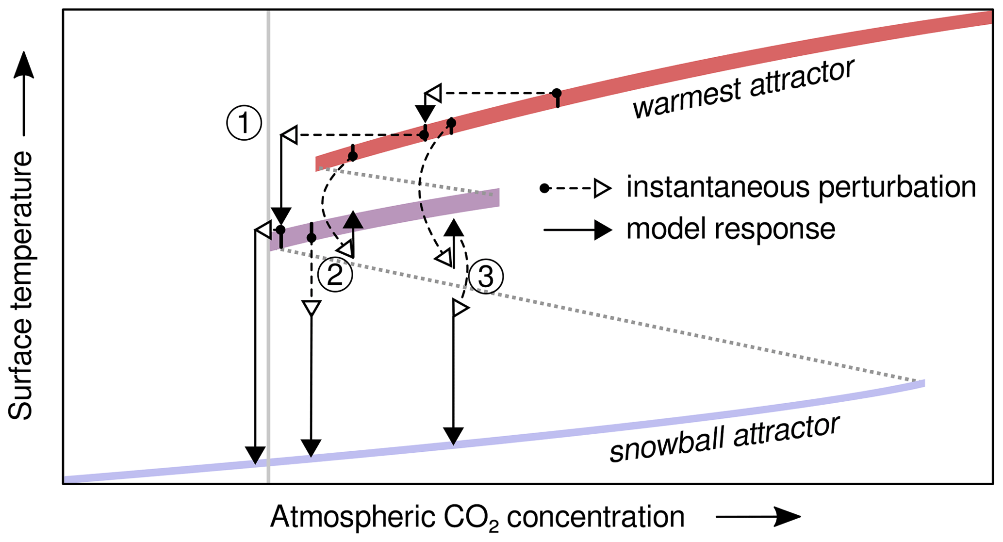
Figure 1Schematic sketch of two non- or partially ice-covered attractors and a snowball attractor (coloured stripes), projected onto the surface-temperature axis, for a range of atmospheric CO2 concentrations. Dotted grey stripes represent intermediate and mostly unstable attractors separating the basins of attraction. In our study, snowball inceptions follow from either ① a stepwise reduction in CO2 (“B-tipping”; Ashwin et al., 2012), ② a single transient perturbation of the surface temperature, or ③ a fast sequence of transient perturbations (“S-tipping” in both cases; Halekotte and Feudel, 2020). For ①, the inception occurs below the equilibrium threshold (vertical grey line). ② and ③ yield snowballs below perturbed thresholds.
There are different frameworks within which to describe such shifts (e.g. Held and Suarez, 1974; Roe and Baker, 2010; Lucarini et al., 2010; Lucarini and Bódai, 2017). Dynamical systems theory, for example, provides the concepts of trajectories along which a particular set of simulated variables moves with time and attractors, which are phase-space regions within which the trajectories stay after some time having constant boundary conditions (e.g. Müller, 2022, their Chap. 4). Essentially, an attractor corresponds to the widely used notion of an equilibrium or steady climate state. Upon approaching a snowball Earth, a stable attractor of partially ice-covered states eventually becomes unstable and vanishes. This qualitative change in the model's phase space, called bifurcation, leaves the system with a snowball state as its nearest attractor. In fact, the snowball and one or multiple other warmer attractors may coexist for a large range of radiative boundary conditions (exemplarily sketched in Fig. 1), with a hysteresis occurring upon changing these conditions.
Possible causes of snowball inceptions and terminations can be investigated with climate models only to a certain degree. Regarding a snowball termination, a gradual buildup of the atmospheric carbon-dioxide (CO2) concentration through volcanism, probably facilitated by reduced weathering in the presence of global ice cover (Walker et al., 1981) and maybe complemented by volcanic dust deposition on the ice (e.g. Abbot and Pierrehumbert, 2010; Abbot and Halevy, 2010; Le Hir et al., 2010), is usually considered a likely cause (e.g. Hoffman et al., 2017). Going from a partially ice-covered to a snowball Earth, a runaway ice–albedo feedback can be triggered either by a significant increase in land-ice extent or by sustained local or global cooling. The long-term effect of dynamic ice sheets on a snowball inception has been tested only occasionally (e.g. Hyde et al., 2000). In contrast, a large number of studies discuss potential causes for sustained cooling or a high Proterozoic susceptibility to glaciation, including the lower solar luminosity (Feulner, 2012; Feulner et al., 2023), a modification of atmospheric-CO2 drawdown due to emerging land plants around 470 Ma (Brady and Carroll, 1994; Pierrehumbert, 2010, their Chap. 8) or carbonate-precipitating plankton (Ridgwell et al., 2003), variations in atmospheric methane (Pierrehumbert et al., 2011), increased reflectivity of clouds (Feulner et al., 2015), the CO2 sequestration resulting from large tropical continents (Hoffman and Schrag, 2002), or the breakup of the supercontinent Rodinia (Goddéris et al., 2003).
Most modelling studies scan for critical radiative conditions, here called equilibrium thresholds, at which the coldest non-snowball attractor vanishes (scenario 1 in Fig. 1; a type of “bifurcation-induced [B-]tipping” as classified by Ashwin et al., 2012). These thresholds are mostly specified as critical values of the solar constant S0 or the atmospheric CO2 concentration, which can vary considerably between different models (Yang et al., 2012a, b, c; Feulner et al., 2023) and depend on different boundary conditions, e.g. ozone concentration (Jenkins, 1999), the degree of desertification (Hoffman et al., 2017), and ocean salinity (Olson et al., 2022).
Another boundary condition on which the bifurcation depends is the distribution of continents on Earth's surface. The continental configuration primarily affects the planetary energy balance via the surface albedo, its influence on the presence of continental ice and snow, and changes in ocean-circulation patterns. In the context of the snowball inceptions during the Neoproterozoic, this has been investigated in a number of studies (e.g. Lewis et al., 2003; Voigt et al., 2011; Liu et al., 2013) using either idealised continental configurations, reconstructions, or the difference between Neoproterozoic and present-day land–ocean distributions. Recently, Merdith et al. (2021) published a new reconstruction of Neoproterozoic continental distributions which has not been used in quantifications of snowball inceptions yet.
One further point we would like to emphasise is that the search for equilibrium thresholds neglects the fact that Earth's climate is subject to additional forcings that cause natural climate variability on a wide range of timescales. For example, periodic changes in Earth's orbital parameters can generate climate variations on timescales of ∼104–105 years, as fluctuations in eccentricity, obliquity, and the timing of the perihelion vary the geographic and seasonal distribution of the incoming solar radiation (Milanković, 1941; Donnadieu et al., 2002). Lewis et al. (2003) found marked differences in climate for two selected orbital configurations under Neoproterozoic boundary conditions, but a more complete range of Earth's orbital parameters are still to be investigated.
On even shorter timescales of ∼1–102 years, single or sequential large volcanic eruptions can cool Earth's climate due to the formation of stratospheric sulfate aerosols (Robock, 2000). In principle, such perturbations are able to trigger a snowball inception below some “perturbed threshold”, a CO2 concentration above the equilibrium threshold (scenarios 2 and 3 in Fig. 1; types of “shock-induced [S-]tipping” from single or sequential large eruptions; Halekotte and Feudel, 2020). The potential role of volcanic eruptions associated with the Franklin Large Igneous Province in triggering the Sturtian glaciation has been investigated by Macdonald and Wordsworth (2017). They argue that the cool climate states of the Neoproterozoic are particularly sensitive to the effects of volcanic eruptions due to the lower tropopause height, which results in a higher sulfate flux to the stratosphere. In a series of simulations, Gupta et al. (2019) explored the ability of single and sequential eruptions to trigger transitions between attractors. A more systematic study of the effect of volcanic eruptions of different magnitudes on the Sturtian and Marinoan snowball-inception thresholds in a coupled climate model is still lacking, however.
Here, we study both the sensitivity of the equilibrium threshold to continental configuration and orbital geometry, i.e. the combination of orbital parameters, and that of the perturbed threshold to volcanism for both Neoproterozoic snowball inceptions in a coupled climate model of intermediate complexity (Montoya et al., 2005). In terms of continental configuration, we test the recent Merdith et al. (2021) reconstructions against earlier ones by Li et al. (2013) as well as more idealised end-member configurations of widely dispersed landmasses and a supercontinent centred at the South Pole, respectively. The sensitivity of the snowball inception with respect to orbital parameters is investigated by sampling the parameter space of Earth-like orbital configurations. Due to the long timescale of Milanković-forcing variations (Milanković, 1941) and the prohibitive computational demands for transient simulations, we do this in terms of equilibrium simulations. Finally, we quantify the perturbed thresholds due to single volcanic eruptions of different magnitudes and with globally homogeneous or zonally resolved aerosol loads as well as the effect of sequential eruptions with realistic statistics.
This paper is organised as follows. In Sect. 2, we describe the model used for our investigation as well as the boundary conditions and sensitivity experiments. The following sections focus on the sensitivity of the Neoproterozic climate system and the snowball inception to continental configuration (Sect. 3), orbital parameters (Sect. 4), and volcanic eruptions (Sect. 5), and we discuss the results in the context of related work. Finally, Sect. 6 summarises our findings.
2.1 Model
As in our earlier investigations of Neoproterozoic glaciations (Feulner and Kienert, 2014; Feulner et al., 2015), we use the relatively fast intermediate-complexity model CLIMBER-3α (Montoya et al., 2005) that enables us to run a large number of simulations. CLIMBER-3α consists of (1) an improved version of the ocean general circulation model MOM3 (Pacanowski and Griffies, 2000; Montoya et al., 2005; Hofmann and Morales Maqueda, 2006) run at a coarse horizontal resolution of with 24 vertical layers, (2) the sea-ice model ISIS (Fichefet and Morales Maqueda, 1997; Hunke and Dukowicz, 1997) operated at the same horizontal resolution and capturing both the thermodynamics and dynamics of sea ice, and (3) the fast statistical–dynamical atmosphere model POTSDAM-2 (Petoukhov et al., 2000) with grid cells measuring 22.5∘ in longitude and 7.5∘ in latitude. CLIMBER-3α does not support waterbelt states with narrow regions of open ocean around the Equator. However, it has been shown to support multiple stable cold climate states with extensive sea-ice cover in an aquaplanet setup (Feulner et al., 2023).
The albedo parametrisations of ice- and snow-covered surfaces can differ significantly between climate models and are known to have crucial effects on snowball inceptions (e.g. Pierrehumbert et al., 2011; Yang et al., 2012c). In our model setup (based on Feulner and Kienert, 2014), bare sea ice has a clear-sky albedo of up to 0.32 for infrared and up to 0.62 for visible and ultraviolet radiation. Snow-covered sea ice has maximum clear-sky albedos of 0.57 and 0.87. For overcast conditions, sea-ice albedos are raised by 0.06. Snow on land has maximum albedos of 0.79 (infrared) and 0.97 (visible and ultraviolet) for clear sky, which are lowered to 0.65 and 0.95, respectively, for overcast sky. Snow albedos decrease depending on snow age, snow temperature, dust cover, and the solar zenith angle. In the absence of ice or snow cover, bare-soil albedos are constant: 0.3 in the infrared and 0.15 in the visible and ultraviolet. Ocean albedos assume values of 0.05–0.2 for clear-sky and 0.07 for overcast conditions, independent of the wavelength.
In addition to the coarse spatial resolution, potential limitations of the model mostly result from the simplified atmosphere component, which statistically captures the large-scale atmospheric circulation patterns rather than simulating weather, the absence of ice sheets, and the missing effects of volcanic ash and dust. Although the large-scale atmospheric circulation dynamically responds to changes in the boundary conditions, some aspects are fixed, in particular the annual-mean width of the Hadley circulation cells (Petoukhov et al., 2000). Since CLIMBER-3α does not include interactive ice sheets, we run the model without any land ice. Despite these two limitations, the resulting equilibrium thresholds for snowball inceptions in the Neoproterozoic fall well within the range derived from more complex models (Feulner et al., 2023). However, the model does not include the transport and deposition of volcanic ash and dust, thereby neglecting their darkening effects on snow. We will discuss the potential impact of model limitations on our results in Sect. 6.
2.2 Simulation setup
According to our research question, we proceed along three different tracks involving simulations with either (1) different continental configurations (Sect. 2.2.1), (2) different orbital geometries (Sect. 2.2.2), or (3) different scenarios of volcanic activity (Sect. 2.2.3 to 2.2.5).
Simulations in (1) and (2) are designed as sets of unperturbed simulations. In the context of this study, “unperturbed” means that we leave the solar constant, the continental configuration, and the orbital geometry unchanged throughout each run and let the model approach an attractor.
Volcanic eruptions are emulated as prescribed transient perturbations of the incoming solar radiation, either globally homogeneous or zonally resolved. Starting from single global perturbations of different magnitudes at three different orbital geometries (Sect. 2.2.3), we proceed to investigate the effects of different latitudes of eruption (Sect. 2.2.4) and sequences of eruptions (Sect. 2.2.5) with reference to the single global eruptions at one particular orbital geometry.
2.2.1 Sampling continental configurations
For each of the two Neoproterozoic snowball-Earth onsets – the Sturtian onset (taken here as 720 Ma) and the Marinoan (here 650 Ma) – four different continental configurations are applied as boundary conditions: (1) two reconstructions and (2) two idealised configurations. Figure 2 shows the distribution of continents and the bathymetry in the different configurations along with the zonally averaged land fraction. The idea behind this sampling is (1) to obtain an estimate of the uncertainty induced by using different realistic palaeogeographies and (2) to roughly cover the largest possible uncertainty of global-mean temperatures caused by the distribution of continents.
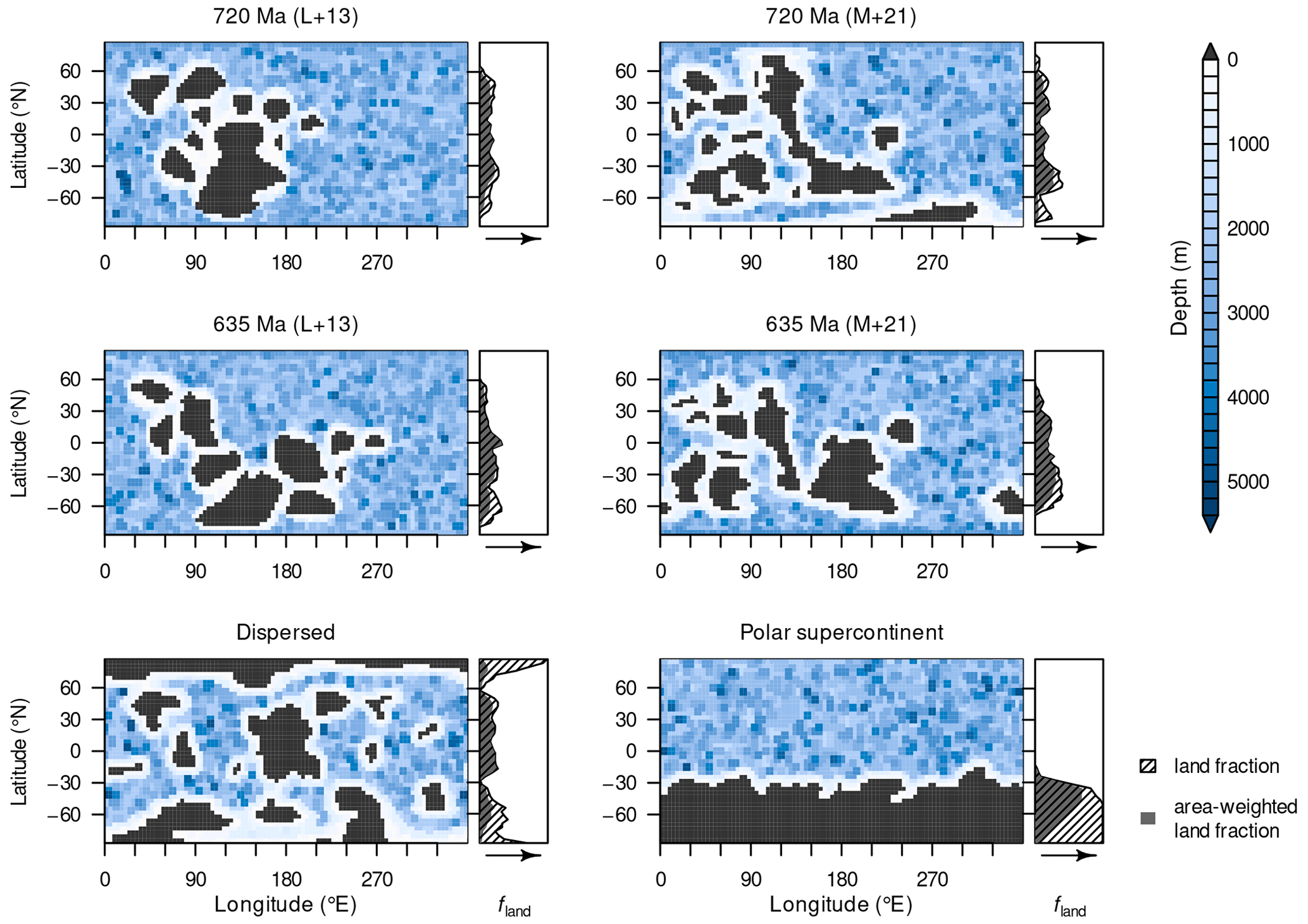
Figure 2Distributions of the exposed continental surface, ocean bathymetry, and zonally averaged land fraction for the different continental configurations. Age specifications (720 and 635 Ma) refer to the time of the reconstructions, L+13 denotes reconstructions based on Li et al. (2013), and M+21 denotes those based on Merdith et al. (2021). Land fractions are shown as simple zonal averages (hatched) and zonal averages weighted by the actual area of the latitudinal bands (grey).
The reconstructions are based on published datasets from Li et al. (2013) and Merdith et al. (2021) dated to 720 Ma for the Sturtian and 635 Ma for the Marinoan snowball onset. (Note, however, that we perform Marinoan simulations with the solar constant at 650 Ma.) These reconstructions rely upon narrowly constrained palaeomagnetic datasets derived from cratonic lithologies as well as plate kinematics and tectonostratigraphic correlations. The more refined methods applied in the Merdith et al. (2021) palaeogeography also allow the trajectories of large terranes to be projected through geologic history, producing a more robust model foundation during a time of hypothesised metamorphism following the breakup of the supercontinent Rodinia (Merdith et al., 2017). For the remainder of the paper, the reconstructions based on Li et al. (2013) will be referred to as L+13, and those based on Merdith et al. (2021) will be referred to as M+21.
The land–ocean masks based on the reconstructions are re-gridded to the ocean-model grid with a horizontal resolution of . Some grid cells have to be manually adjusted, for example to avoid isolated ocean cells within continents or narrow ocean channels. For the L+13 reconstruction, continental shelves and slopes with a typical width of one ocean grid cell each are assigned by hand around all land areas (Feulner and Kienert, 2014). For the M+21 reconstruction and the idealised configurations, we use an automatic procedure with shelves and slopes with a width of 500 km each. Ocean depth levels are randomly assigned and fall within the range 100–265 m for continental shelves, 349–993 m for continental slopes, and 1243–4987 m for the abyss. Land cells are set to either a constant elevation of 200 m or randomly distributed elevations between 200 and 400 m. Land-surface type is assumed to be bare soil unless there is snow cover.
The idealised continental configurations are constructed by shifting continental plates of the 635 Ma reconstruction by Merdith et al. (2021) using the GPlates program (Müller et al., 2018) and by subsequently performing the manual adjustments described above. We construct a “dispersed” configuration of small continents distributed evenly over the surface and a “polar supercontinent” configuration, where the single continent is the only landmass and is centred at the South Pole of the model grid. Depth levels of continental shelves, slopes, and deep-ocean cells are assigned in the same manner as for the M+21 reconstruction described above.
The use of different sources and the manual adjustments come with variations in the exposed continental-surface area. This is lower for the reconstructions, with the 720 Ma land fraction (L+13: 16.8 %, M+21: 17.1 %) being smaller than that at 635 Ma (L+13: 17.4 %, M+21: 20.0 %). The idealised dispersed configuration has a land fraction of 20.8 %, and that for the supercontinent is 24.1 %.
Table 1Overview of the simulations regarding the sensitivity to continental distribution, differentiating between those aimed at the temperature sensitivity at fixed CO2 concentration and those aimed at the CO2 threshold for snowball inception. All simulations are initialised in a warmer climate than the shown equilibrium states and are run with an orbital geometry of 23.5∘ obliquity and zero eccentricity. S0 is the solar constant. “L+13” denotes reconstructions based on Li et al. (2013); “M+21” denotes those based on Merdith et al. (2021).
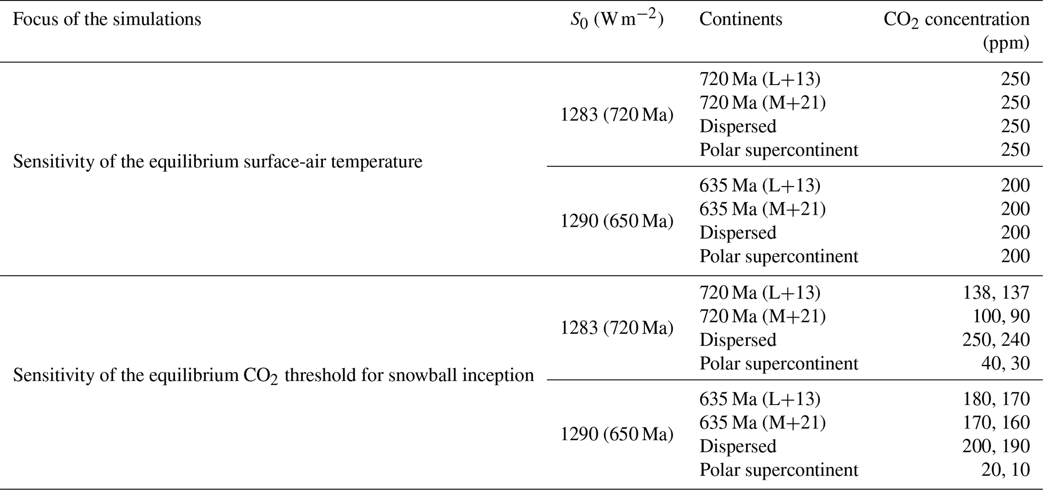
Table 1 provides an overview of the simulations with differing continental configurations. We use the solar constant S0=1283 W m−2 for the Sturtian and 1290 W m−2 for the Marinoan onset. Both values are derived from a standard solar model (Bahcall et al., 2001) using a present-day value of 1361 W m−2. For the orbital geometry, we select an obliquity of 23.5∘ and zero eccentricity. All unperturbed runs are initialised in a warm and ice- and snow-free state with a global-mean surface-air temperature of around 12 ∘C.
In the simulations aiming at a comparison of the energy-balance effects from differing continental distributions, we run the model with an atmospheric CO2 concentration of 250 parts per million by volume (ppm) for the Sturtian and 200 ppm for the Marinoan conditions. Non-CO2 greenhouse gases are not considered in our simulations. Scanning for the CO2 threshold is done by letting the model approach equilibrium for various CO2 concentrations in steps of 10 ppm.
2.2.2 Sampling orbital geometries
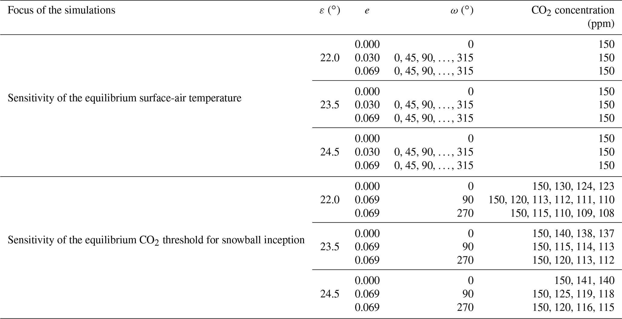
In CLIMBER-3α, the incoming top-of-atmosphere solar radiation is determined by three orbital parameters: obliquity ε, eccentricity e, and argument of perihelion ω. corresponds to perihelion at the September (southward) equinox and to that at the December (southern) solstice. We sample the ε–e–ω parameter space by selecting the coordinates ε= (22, 23.5, 24.5∘), e=(0, 0.03, 0.069), and ω= (0, 45, 90, 135, 180, 225, 270, 315∘) and running the model for selected physically distinguishable combinations thereof. (Note that for e=0, the different values of ω are indistinguishable in terms of the annual and seasonal distributions of insolation.) The ranges of ε and e are confined by computations of Earth's orbital variations during the past 250 million years (Laskar et al., 2004). The climate in these simulations is initialised in the same way as for the set of simulations described above.
An overview of the simulations with varying orbital geometries is given in Table 2. For all 51 distinguishable configurations, we run the model at a CO2 concentration of 150 ppm in order to compare the effects of orbital geometry on the surface-air temperature. Since these effects are significantly smaller than those of the continental configurations, we perform finer scanning for the CO2 thresholds at nine different orbital geometries: after letting the model approach a steady state, which usually takes around 1000–3000 years, we reduce CO2 by 1 ppm – or more if it is well above the threshold – and repeat this procedure until we have a snowball inception in each simulation. The continents and solar constant always correspond to the Sturtian onset (720 Ma) using the respective L+13 continental reconstruction.
Table 2Overview of the simulations regarding the sensitivity to orbital geometry, differentiating between those aimed at the temperature sensitivity at fixed CO2 concentration and those aimed at the CO2 threshold for snowball inception. All simulations are initialised in a warmer climate than the shown equilibrium states, run at a solar constant of 1283 W m−2, and use the Sturtian L+13 palaeogeography. ε is the obliquity, e is the eccentricity, and ω is the argument of perihelion.
2.2.3 Sampling single global volcanic perturbations
We implement globally averaged volcanic perturbations as annually resolved transient variations in the solar constant. The radiative perturbation resulting from a single explosive eruption is idealised as follows: in the calendar year after the eruption, the perturbation reaches a peak forcing, which is followed by an exponential decrease (, where the decay rate λ has a value of 1 yr−1) in successive calendar years ti. In the calendar year of the eruption, the forcing is half the peak forcing, representing a linear buildup due to sulfate aerosols being injected into the stratosphere. This form of the perturbation, including the value of λ, is commonly used in the literature (e.g. Ammann et al., 2003; Gao et al., 2008; Metzner et al., 2014).
With the aim of sampling the peak forcing realistically, we construct our idealised scenarios by following ice-core-based reconstructions of the net solar radiative forcing ΔSnet(t) due to volcanism during the years 850–2000 common era (CE; Schmidt et al., 2012, based on Gao et al., 2008, and Crowley et al., 2008) as well as model-based forcings of the ∼ 74 000 a Toba (Timmreck et al., 2010) and 2.1 Ma Yellowstone eruptions (Segschneider et al., 2013). The annual- and global-mean peak forcings from these reconstructions cover a range of up to −20 W m−2. We define our single-eruption scenarios using a nominal reduction of the global-mean net solar radiation, here called “nominal volcanic forcing” (NVF), with peaks of −2, −5, −10, −20, −30, and −40 W m−2, thus also allowing for what we consider extreme and very rare perturbations beyond the reconstructions. Note that some previously applied (Jones et al., 2005; Robock et al., 2009; Gupta et al., 2019) estimates of the ∼ 74 000 a Toba eruption exceed a peak forcing of −100 W m−2 but have been criticised on physical grounds as being much too strong (Timmreck et al., 2010, 2012).
The translation of a given NVF to a change in the solar constant results from a basic consideration of the top-of-atmosphere short-wave radiation balance: the daily- and zonal-mean net solar radiation is , where ϕ is the latitude, A is the planetary coalbedo (1−albedo), g is a factor comprising geometric effects of Earth and its orbit, and ϕz is the latitude at which the Sun reaches the zenith at noon (e.g. Peixoto and Oort, 1992, their Sect. 6.3.2). For the annual and global mean, denoted by an overline, we approximate by , where Aeff is a geometry- and radiation-weighted effective global coalbedo and (Berger and Loutre, 1994). We use the present-day global coalbedo of 0.7 (Goode et al., 2001) as an estimate for Aeff. Thus, we translate the NVF into the solar-constant forcing ΔS0 via
where ti represents successive calendar years.
Three comments on the construction of the volcanic forcing are appropriate at this point. First, the volcanic forcing is called “nominal” here because, in this construction, each eruption corresponds to a reduction in the solar constant of around 5.7 NVF for the used eccentricity range, independent of the actual climate state. This means that, while the NVF represents the volcanic effects in a Quaternary or modern climate, the actual reduction in the net solar flux is somewhat smaller in a colder climate with a lower coalbedo. For the sake of simplicity and comparability with other studies, however, we continue to specify the eruption scenarios using the NVF.
Second, the use of annual reductions in the solar constant implies that volcanic eruptions always start at the beginning of a calendar year, i.e. in northern-hemispheric winter.
Third, Macdonald and Wordsworth (2017) argued on the basis of a vertical atmospheric and volcanic-plume model that volcanic eruptions can have a particularly strong impact on snowball inceptions because the tropopause, the lower boundary of the stratosphere, is generally lower in cooler climates. We do not explicitly include such an effect here.
All perturbed runs, including those described in the sections below, have Sturtian boundary conditions, making use of the respective L+13 palaeogeography. Only single global perturbations are tested for different orbital geometries, which are {, e=0}, {, e=0}, and {, e=0.069, }. See Table 3 for an overview of these simulations.
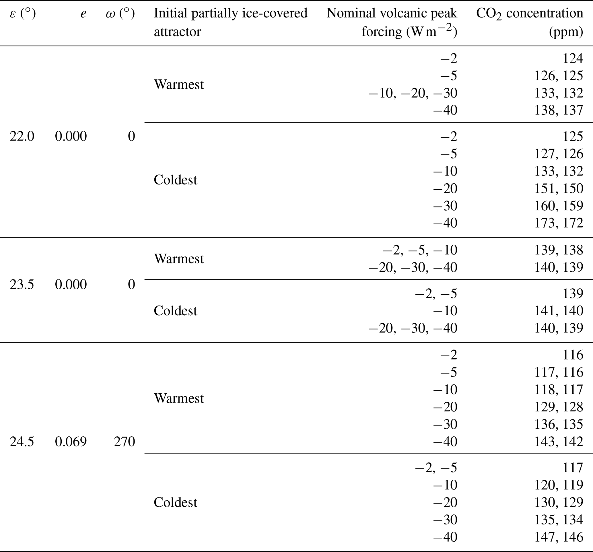
Table 3Overview of the simulations regarding the sensitivity of the CO2 threshold for snowball inception to single global volcanic perturbations. All simulations are run at a solar constant of 1283 W m−2 and use the L+13 palaeogeography for 720 Ma. ε is the obliquity, e is the eccentricity, and ω is the argument of perihelion. The “initial partially ice-covered attractor” refers to the conditions at which a particular simulation was initialised.
2.2.4 Sampling single zonal volcanic perturbations
To emulate the latitudinally resolved effects of large volcanic eruptions, we prescribe a transient zonal distribution of aerosol optical depth (AOD) yielding a proportional reduction in the solar constant at each latitude band. The aerosol time series are taken from Ammann et al. (2003), who estimated the monthly and zonally resolved AODs for historical eruptions between 1890 and 1999 CE based on a simple model of sulfate-aerosol transport in the stratosphere. We exemplarily select periods of 6–9 years including and following three eruptions at different latitudes: the 1902 Gagxanul/Santa María eruption (at 15∘ N), the 1932 Quizapú/Cerro Azul eruption (36∘ S), and the 1912 Novarupta eruption (58∘ N). We interpolate these data to our atmospheric grid and prolong them to cover 50 years, assuming exponential decay at a rate of 1 yr−1 after the last available values (Appendix Fig. A1). Additionally, we flip the data at the Equator to eventually get AOD time series for eruptions at 15, 36, and 58∘ in both hemispheres.
In order to produce comparable results, we scale the AOD data for each peak forcing in such a way that the global-mean reduction in the solar constant integrated over 50 years is equal to the 50 year integral of ΔS0(t) for the respective global volcanic perturbation described above. Regarding their effects on the model response, the only differences from the global perturbations are the finer spatial (latitudinal) and temporal (monthly) resolution. Note in particular that, as in the global case, eruptions always start in January.
All zonal perturbations are initialised on both the warmest and the coldest partially ice-covered attractors for the orbital geometry {, e=0}. See Table 4 for an overview.
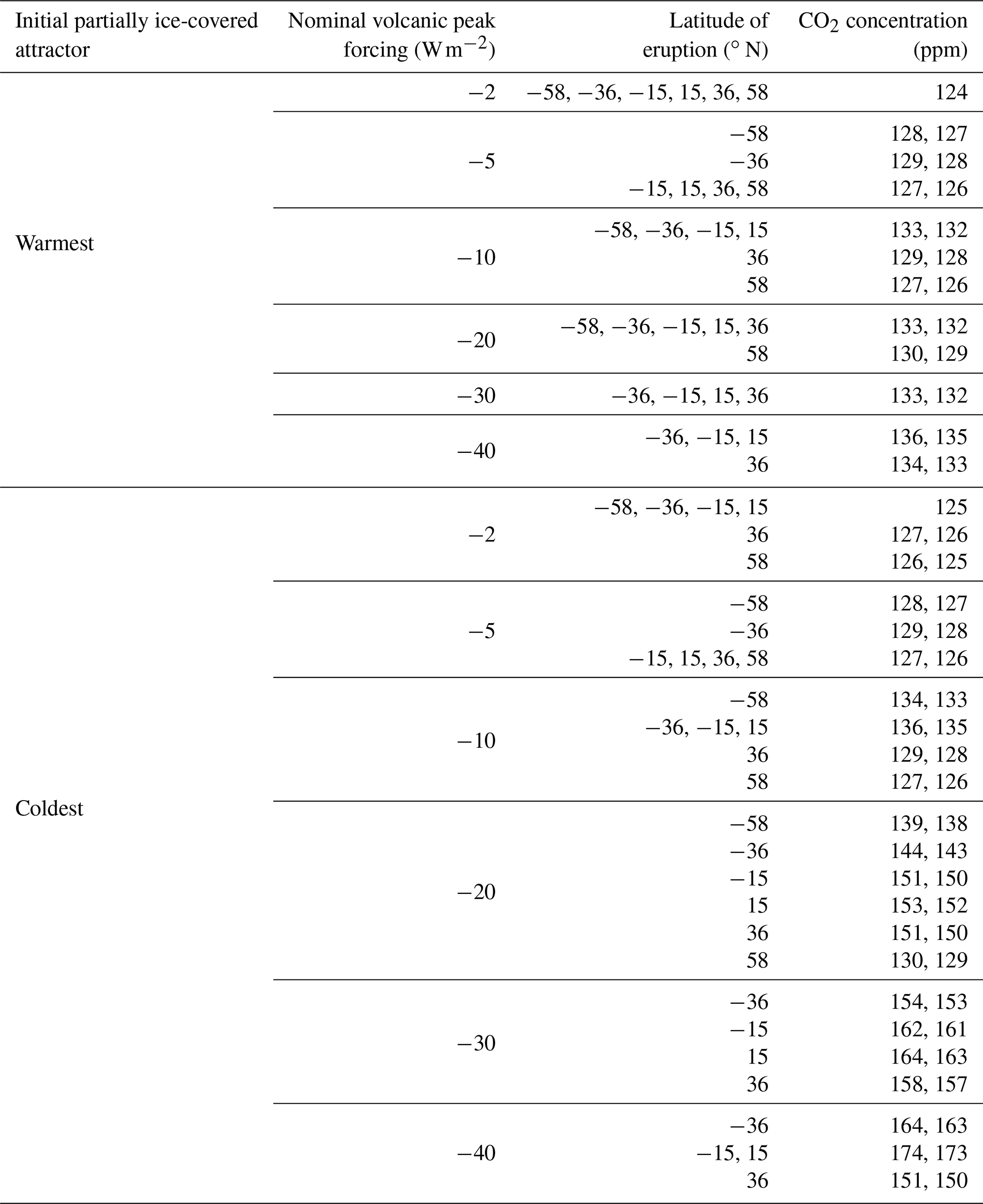
Table 4Overview of the simulations regarding the sensitivity of the CO2 threshold for snowball inception to single zonal volcanic perturbations. All simulations are run at a solar constant of 1283 W m−2, use the Sturtian L+13 palaeogeography, and have an orbital geometry of 22∘ obliquity and zero eccentricity.
2.2.5 Sampling sequences of global volcanic perturbations
We generate sequences of global volcanic perturbations along the lines of Ammann and Naveau (2010), who construct such annual-mean time series based on two processes, one purely stochastic and one purely deterministic.
First, the occurrence of explosive eruptions ejecting sulfate aerosols into the stratosphere is modelled as a stochastic annual time series bp(ti) consisting of binary values (“no eruption” or “eruption”, i.e. a Bernoulli process), where “eruption” has the constant probability p and “no eruption” has the probability 1−p. Each such eruption is then assigned a nominal volcanic peak forcing Π(ti) randomly drawn from a generalised Pareto distribution with probability density
where β>0, ξ are real numbers, u and x are given in W m−2, u > x, and the term in brackets is positive. This function asymptotically describes excesses over large thresholds of many probability distributions (Embrechts et al., 1997), including the peak radiative forcing of large volcanic eruptions (Naveau and Ammann, 2005). Note that in our case, the distribution describes negative events x beyond a negative threshold u. The nominal volcanic forcing, i.e. reduction of the net solar radiation, is translated into a reduction in the solar constant in the same way as described in Sect. 2.2.3. The complete first process, describing subsequent peaks Σ in the perturbation of the solar constant, therefore reads
where “d” over the equality sign implies equality in distribution.
Second, each peak is followed by an exponential decay as in our idealised single perturbations, which is described by the deterministic process .
Both processes are combined, yielding the max-autoregressive model
Taking the maximum each year instead of the sum ensures that the effective distribution of peak forcing follows the distribution , even for overlapping events.
The values of the parameters p, β, ξ, and u (characterising the frequency of eruptions and the distribution of peak forcings) define our scenarios. Roughly oriented towards the assumptions and parameter-fitting results by Ammann and Naveau (2010), we define the reference scenario as {p=0.1, β=1, ξ=0.3, u=1.5 W m−2}, which reproduces the volcanic-forcing statistics of the past ∼ 1000 years by and large. Based on this scenario, we subsequently change one parameter at a time in order to define five more scenarios. They comprise raising the eruption probability p to 0.3, varying the shape parameter β between 0.5 and 1.5 (a slightly wider range than in Ammann and Naveau, 2010), and shifting the threshold u to 0 and −3 W m−2 (as in Ammann and Naveau, 2010). Tripling the probability of eruptions with a relevant radiative effect is an attempt to represent periods of more frequent volcanic activity, e.g. during the formation of large igneous provinces (LIPs) such as the Franklin LIP related to the Sturtian snowball inception by Macdonald and Wordsworth (2017). While u=0 W m−2 should be only seen as a theoretical case because the generalised Pareto distribution is usually applied for nonzero thresholds (Naveau and Ammann, 2005), W m−2 is chosen as the other limiting case since some effects can already be seen from a peak forcing of −2 W m−2, as reported in Sect. 5.1. Changing ξ within or slightly beyond the range reported in Ammann and Naveau (2010) results in distributions very similar to some scenarios obtained from varying β and u. We therefore chose to leave it fixed at ξ=0.3 for all scenarios, yielding a Fréchet-type distribution with heavy tails (Embrechts et al., 1997).
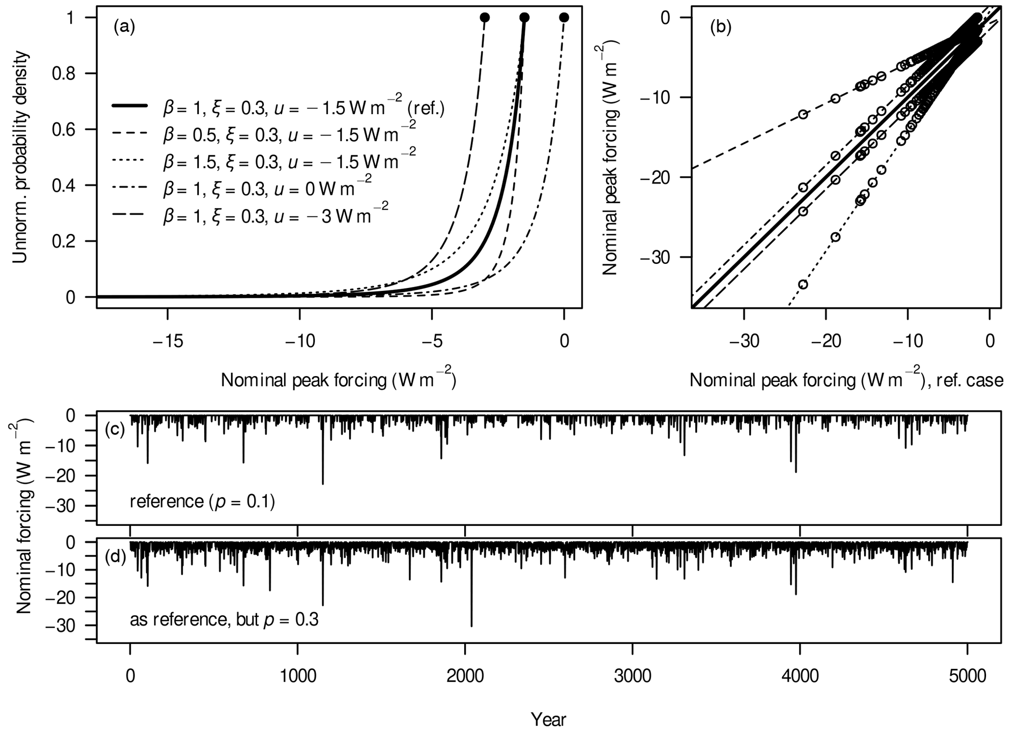
Figure 3(a) Different forms of the generalised Pareto distribution determining the nominal peak forcing in the max-autoregressive model, which are displayed as unnormalised probability-density functions, i.e. they have a maximum value of 1. Dots denote the upper limits of each function's domain and range. For example, the function with W m−2 allows for peak forcings at or below −3 W m−2 only, while all functions are unbounded from below. (b) Nominal peak volcanic forcing in the simulations with each of the distributions from panel (a) compared to the reference scenario (diagonal line) at each time step of the generated volcanic time series. (c) Nominal volcanic forcing in the reference scenario. (d) Same as panel (c) but for the scenario with increased eruption probability.
Figure 3a shows the five different parametrisations of . In order to make the interpretation of results easier, we compute the pseudorandom sequences with a length of 5000 years for all different scenarios based on the same seed, i.e. initial algorithm state. Upon plotting the peak forcings of the reference scenario against the peak forcings from other scenarios for each time step (Fig. 3b), we can see that there are perfect correlations across the time series. Moreover, we can clearly characterise the effects of changing β and u: through the scaling effect of β, the scenarios yield dramatically different forcings for the rarest events, while u shifts the forcings homogeneously and thereby has the strongest effects on the most frequent eruptions, i.e. the “background noise”. Due to the construction, the scenario with an increased eruption probability p contains almost all of the individual events, including their magnitudes, from the reference case but adds many additional events (Fig. 3c, d). The background noise is strongly intensified, leading to a nearly permanent effect of volcanoes on the radiative balance. Additionally, this scenario contains a peak forcing (at around the year 2000 in Fig. 3d) that goes beyond the largest forcing in the reference scenario.
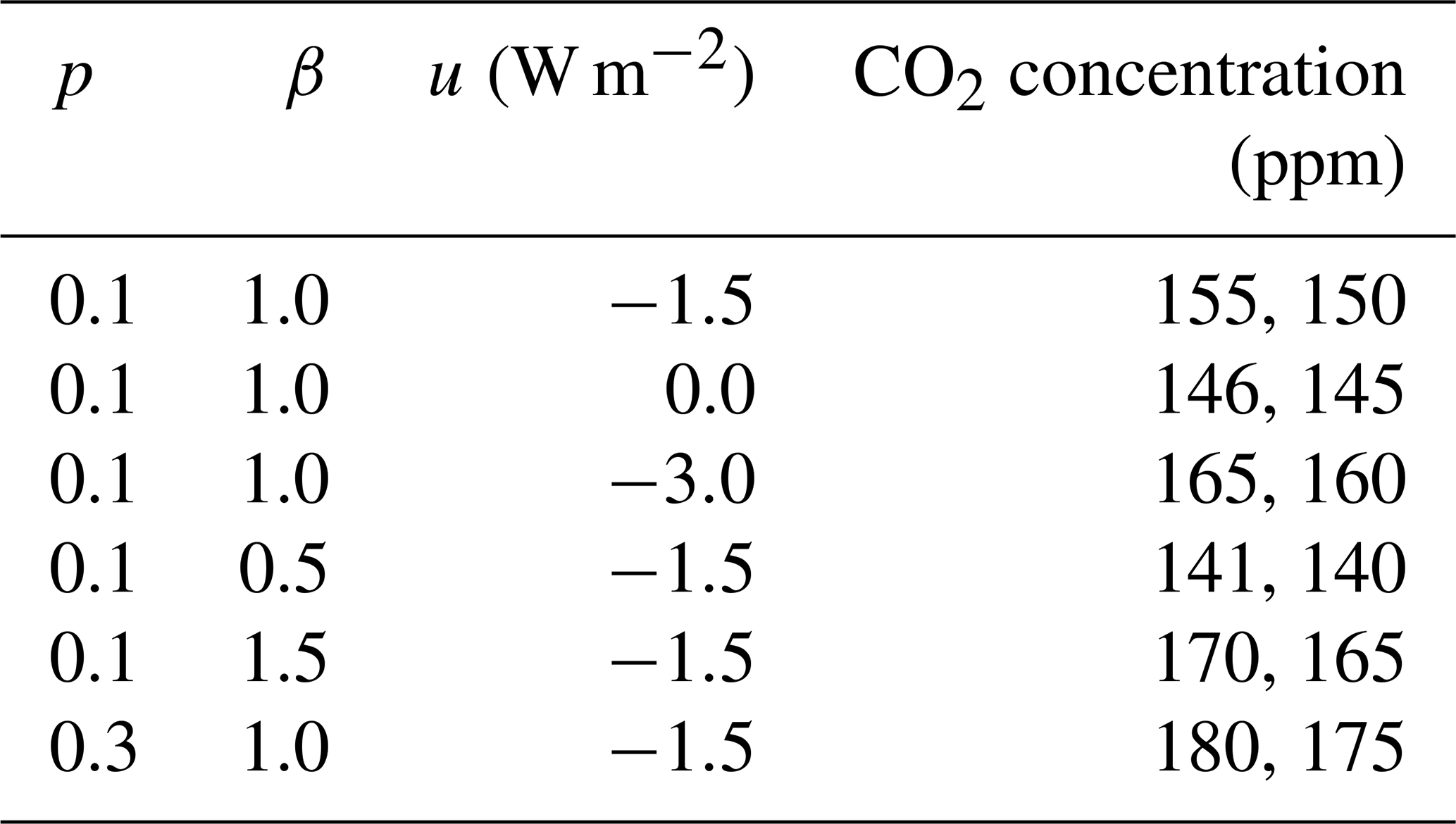
Table 5Overview of the simulations regarding the sensitivity of the CO2 threshold for snowball inception to sequential volcanic perturbations. All simulations are run at a solar constant of 1283 W m−2, use the Sturtian L+13 palaeogeography, have an orbital geometry of 22∘ obliquity and zero eccentricity, and are initialised on the warmest attractor supported at the respective CO2 concentrations.
All simulations are initialised on the warmest partially ice-covered attractors with an orbital geometry of {, e=0}. The reason for choosing only the warmest attractors is that in many simulations, the sequential perturbations force the model from the warmest to the coldest attractor. In these cases, the thresholds would become the same as for simulations initialised on the coldest attractors. In other words, the volcanic “noise” seems to connect the multiple stable states and push the model towards the coldest one. After applying the volcanic forcing for 5000 years, we let the model run without perturbations for 1000 years in order to ensure that we do not miss an eruption-induced transition to a snowball state. Table 5 summarises the simulations with sequential volcanic perturbations.
2.3 Estimating energy-balance contributions to surface-temperature differences
Following an idea first deployed by Heinemann et al. (2009) and later used by Voigt (2010), Voigt et al. (2011), and Liu et al. (2013), we can divide the zonal-mean surface-temperature differences between two equilibrium states into contributions associated with terms of the zonal energy balance. Similarly to the classic energy-balance models, the instantaneous zonal-mean energy balance of an attractor state reads
where Snet is the net solar (short-wave) flux, L the net outgoing terrestrial (long-wave) flux, ∇ϕF the divergence of meridional sensible and latent heat fluxes, and δ represents the fluctuating energy imbalance. All variables represent zonal averages. Parametrising the outgoing thermal radiation as , where W m−2 K−4 is the Stefan–Boltzmann constant, ϵ is the effective emissivity, and T is the surface temperature, and taking the long-term mean (〈⋅〉) yields
where, due to the definition of the attractor and assuming ergodicity, 〈δ〉(ϕ)=0 for all ϕ. If we approximate 〈ϵT4〉≈〈ϵ〉〈T〉4, we obtain the long-term and zonal mean surface temperature as
In the model experiments, the single terms are diagnosed as
where the subscript TOA refers to the top of atmosphere and the subscript s to the surface. Due to the assumption L∝T4 and the approximation in the long-term average, we introduce a systematic error into the computation of the surface temperature. However, Voigt (2010) argues that the error is acceptably small for the typical case that and for the usual surface temperatures. Comparing the surface temperatures from the energy-balance diagnostics with the model output, we find only small differences, the largest of which occur around the poles, as exemplarily shown in Fig. A2.
The surface-temperature difference between some equilibrium states A and B due to changes in net solar flux – comprising a differing solar constant, distribution of insolation, and albedo – can then be computed as
while that due to changes in heat-flux divergence can be computed as
and that due to changes in effective emissivity can be computed as
For the interpretation of these different contributions, it is helpful to realise that changes in the boundary conditions may well reduce or increase the net short-wave or long-wave radiation globally, leading to global-mean cooling or warming. In contrast, due to the construction of the balance shown in Eq. (1), the heat-flux divergence vanishes in the global average (e.g. North and Kim, 2017, their Sect. 5) and can thereby only affect the global-mean temperature via local changes and subsequent feedback effects affecting the short-wave or long-wave radiation.
3.1 Surface temperatures
Under Sturtian boundary conditions, the surface-air temperature is distinctly dependent on the continental configuration (Fig. 4), with globally and annually averaged values ranging from −8.9 ∘C in the ideal dispersed configuration to 3.9 ∘C in the southern-hemispheric (SH) polar-supercontinent configuration at an atmospheric CO2 concentration of 250 ppm. The M+21 and L+13 reconstructions adopt intermediate climate states, with values of −1.7 and 0.3 ∘C, respectively. Apart from the direct comparison between the reconstructions, there is a negative correlation between tropical land area and global-mean surface temperature, which is consistent with previous studies (e.g. Voigt et al., 2011).
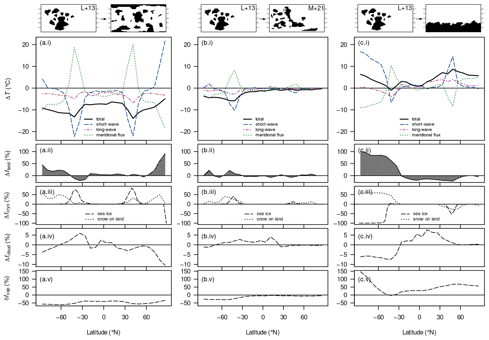
Figure 4Absolute differences in surface temperature ΔT (a(i)–c(i)), land fraction Δfland (a(ii)–c(ii)), land-snow and sea-ice fraction Δfcryo (a(iii)–c(iii)), and cloud fraction Δfcloud (a(iv)–c(iv)) and relative difference in column water vapour (a(v)–c(v)) between long-term-averaged attractor states upon changing the continental configuration for the Sturtian onset. Shown in (a(i))–(c(i)) are the total temperature difference and differences due to changes in net solar radiation (“short-wave”), emissivity (“long-wave”), and meridional heat-flux divergence (“meridional flux”). Differences were computed with reference to the L+13 720 Ma reconstruction (the subtrahend). The solar constant is always 1283 W m−2 (720 Ma); the CO2 concentration is 250 ppm.
Simulations applying boundary conditions representative of the later Marinoan event – at a CO2 concentration of 200 ppm – can attest to these observations. For example, as with the Sturtian simulations, the dispersed and SH supercontinent configurations demonstrate extreme globally and annually averaged surface temperatures of −9.0 and 3.6 ∘C, respectively. The reconstructions once again adopt intermediate climate states, with temperatures of −6.7 and −1.8 ∘C for the M+21 and L+13 palaeogeographies, respectively. The greater discrepancy between the reconstructions of the Marinoan as opposed to the Sturtian is potentially a result of the greater degree of dispersion present in the M+21 palaeogeography in the Marinoan glacial event due to the continued separation of the supercontinent Rodinia (Hoffman et al., 2017; Liu et al., 2013).
As noted before, the global land fraction slightly differs between the continental boundary conditions, which needs to be ruled out as a governing effect before discussing the individual energy-balance contributions. A small number of comparison simulations at 720 Ma with a manually adjusted land fraction of ∼17 % for all configurations (not shown) exhibit effects on the surface-air temperature (the slight increase in continental area in the dispersed configuration even yields a snowball at 250 ppm) but leave the order of temperatures and critical CO2 concentrations among the boundary conditions unchanged.
3.1.1 Dispersed configuration versus L+13 configuration
Let us now look at the individual energy-balance components (net solar radiation, meridional heat flux, and long-wave emission) in order to understand the large difference in surface temperature between the dispersed configuration and the Sturtian L+13 reconstruction (Fig. 4a(i)–(v)). The former case is significantly colder due to a great influence of the changed net solar radiation, i.e. albedo, and a minor effect of the increased global emissivity; see Fig. A3 for the global contributions. Changes in the meridional heat flux mostly act to compensate for zonal changes in the surface temperature caused by the other energy-balance components. When considering global averages, the meridional heat flux has virtually no effect on the surface temperature (Fig. A3), as anticipated in Sect. 2.3. We now proceed to discuss the components in more detail.
Since neither the solar constant nor the distribution of insolation is changed between the compared setups, differences in net solar radiation only represent albedo effects. These effects can already be detected in the spin-up of the simulations (not shown): after initialisation with nearly identical climatic conditions, the higher albedo and lower thermal inertia of high-latitude continents in the dispersed configuration lead to a strong cooling effect amplified by snowfall over land. As the simulations progress, the climate of the dispersed configuration consistently remains cooler than that of the L+13 reconstruction. Finally, upon ice margins encroaching into the mid-latitudes, the slightly larger continental area in the tropics further supports the cooler conditions in the dispersed case, favouring snowfall even there. At equilibrium, the most drastic differences in surface temperature occur over the sea-ice margins (Fig. 4a(i)). The cooling peaks at around 40∘ S/N in the short-wave contribution are correlated with the differences in cryosphere fractions (Fig. 4a(iii)) and are likely the results of ice–albedo feedbacks at the ice margins. At the poles, the short-wave contribution yields higher temperatures in the dispersed configuration, where the presence of continents prevents the formation of sea ice and there is insufficient snowfall to compensate for the change in albedo.
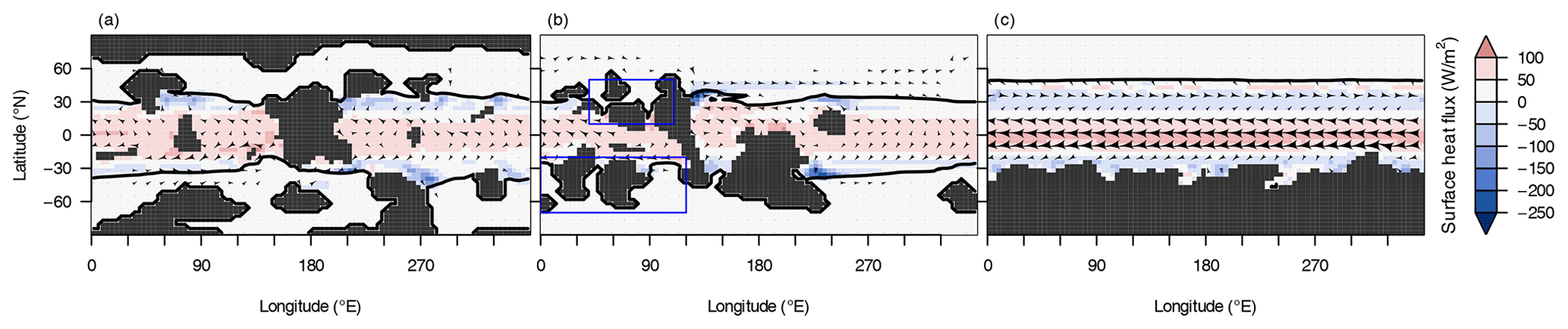
Figure 5Long-term-mean sea-ice cover (50 % contours shown as thick black lines), surface ocean velocity (arrows with lengths proportional to the velocity), and heat flux at the ocean surface (colours; positive values indicate that the ocean gains heat) for Marinoan (650 Ma) equilibrium simulations using the dispersed (a), M+21 (b), and polar-supercontinent (c) configurations. The CO2 concentration is 200 ppm (a), 170 ppm (b), and 20 ppm (c). Blue rectangles in panel (b) indicate ocean regions featuring local sea-ice protrusions.
Changing the continental configuration can cause changes in the ocean circulation responsible for the meridional heat transport from lower to higher latitudes in the oceans (e.g. Jenkins, 1999), as also seen for modern-day analogies such as the role of the North Atlantic Current in the ocean temperatures of western Europe (Palter, 2015). Such changes can result in regional temperature effects which are difficult to detect in the zonal averages which are shown in Fig. 4. For the dispersed configuration, the ocean-surface currents are both diverted from the Equator and slowed down as compared to the open ocean in the supercontinent configuration (shown in Fig. 5a and c for the Marinoan conditions before snowball inception). The situation is similar for the heat transport between the Equator and the ice margins in the L+13 configuration (not shown).
Differences in emissivity, i.e. the greenhouse effect, within the modelled climate appear to have a localised influence that is dependent on the surface temperature and primarily due to the water-vapour feedback: the lower temperature in the dispersed configuration causes increased rates of evaporation and atmospheric concentrations of water vapour, again yielding lower temperatures. This demonstrates that emissivity is affected by the continental distribution indirectly and is a result of a feedback rather than an initial cause of cooling or warming. The influence of emissivity on the global climate can be investigated further by distinguishing the localised influences of cloud fraction and water vapour. A comparison of Fig. 4a(i), (iv), and (v) demonstrates that the water-vapour concentration strongly affects the long-wave emission, which is further modulated by cloud cover. Over the poles, the reduced cloud cover contributes to a cooling from reduced emissivity, which exceeds the warming from reduced ice cover.
A comparison of the dispersed configuration with the Marinoan L+13 reconstruction shows a very similar overall picture (Figs. A4 and A5). The general tendency for cooling in a dispersed configuration is corroborated by Hyde et al. (2000), who adopted boundary conditions including a SH supercontinent originally derived by Dalziel (1997). By increasing the degree of dispersion between the continents, Hyde et al. (2000) note that the threshold atmospheric CO2 concentration for a snowball inception is increased.
3.1.2 M+21 configuration versus L+13 configuration
The Sturtian L+13 and M+21 reconstructions differ by 2 ∘C regarding their global-mean surface temperatures, with the M+21 configuration being the colder one. This difference is mainly caused by SH albedo differences and amplified by emissivity changes (Figs. 4b(i)–(v) and A3).
The largest difference in zonally averaged land fraction between the two configurations is found in middle and higher latitudes of the Southern Hemisphere, where we also observe a pronounced increase in snow- and sea-ice cover. The cooler Southern Hemisphere is therefore likely a result of the increased continental area.
For the Marinoan simulations, the overall picture is very similar, but surface temperatures in the L+13 and M+21 reconstructions differ more strongly, mainly due to albedo differences (Fig. A5). Considering zonal averages (Fig. A4b(i)–(v)), the Marinoan configurations show larger local absolute differences in continental area and cryosphere fractions than the Sturtian equivalents. Additionally, the slightly greater low- and middle-latitude landmass area present in the Marinoan M+21 relative to the L+13 reconstruction reduces the absorption of solar radiation between the sea-ice margins.
For both the Sturtian and the Marinoan, the emissivity and meridional heat flux reflect the zonal cooling or warming caused by albedo differences. Nevertheless, the Marinoan M+21 configuration provides an example of local protrusions in the sea-ice front: due to the positioning of continental clusters, several middle-latitude ocean parts between 0 and 120∘ E are secluded from ocean currents and, without an influx of warmer equatorial water, adopt a cooler regional climate (blue rectangles in Fig. 5).
3.1.3 Polar supercontinent configuration versus L+13 configuration
The SH polar supercontinent stands out as the warmest configuration (Figs. 4 and A3). Again, the largest part of the temperature difference in comparison to the Sturtian L+13 configuration results from net short-wave differences (Fig. A3c(i)–(v)). Almost the entire supercontinental domain has surface temperatures of several degrees, with the warming due only to albedo changes. The differences in cryosphere fractions (Fig. 4c(iii)) imply that it is the absence of sea ice which increases the albedo, despite the presence of snow on land.
Apart from the albedo, the difference in meridional heat transport seems to play an important part: the continental margin obstructs equatorial heat from bypassing a latitude of S via ocean currents. The resulting warming in this zone exceeds the cooling from snow cover. This enforces a decreased temperature reduction during the SH winter months, minimising sea-ice advancement between the Equator and 30∘ S due to the stored thermal energy, as illustrated in Fig. 5c. Note that this configuration is not represented anywhere in geologic history, and so this mechanism likely does not elucidate any climate phenomenon currently under study.
Emissivity changes only partly reflect a simple water-vapour feedback. Over the supercontinent, cloud cover is homogeneously lower than in the L+13 configuration and gives rise to increased long-wave emission. This effect is compensated for by increased water-vapour concentrations only over the South Pole. Despite this cooling through long-wave radiation, most of the Southern Hemisphere is warmer in the supercontinent configuration, and the warmer conditions in the Northern Hemisphere (NH) can be partly explained by an ice–albedo feedback around the sea-ice margin. Perhaps another reason for the warmer NH climate is the absence of snow on land.
Very similar observations can be made for Marinoan conditions (Figs. A4 and A5).
3.2 Equilibrium thresholds
The susceptibility of Earth with a particular continental configuration to a global glaciation is also reflected in the critical CO2 threshold, i.e. the highest atmospheric CO2 concentration at which a snowball inception occurs, which is shown together with the coldest non-snowball state for each configuration in Fig. 6. There is a correlation between these thresholds and the surface-air temperature for given CO2 concentrations. This result is plausible because a colder climate state typically features a larger sea-ice extent – and should therefore be closer to some glaciation threshold – than a warmer state, given that both configurations share the same critical sea-ice extent necessary for a snowball inception. Contradicting this expectation, however, we find the M+21 to be more resistant to global freezing than the warmer L+13 reconstructions at both the Sturtian and the Marinoan onsets. The cause is a stable sea-ice extent with margins around the Hadley-cell boundaries (“Hadley state”, Feulner et al., 2023), which is supported in the M+21 configuration but unstable in the L+13 case (insets in Fig. 6).
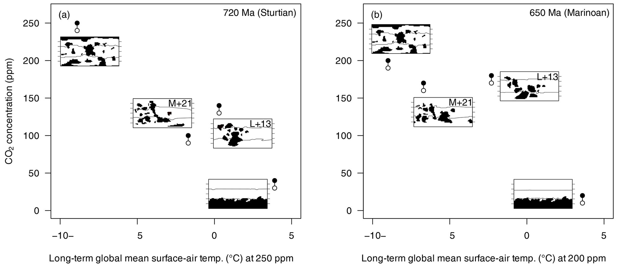
Figure 6Long-term global mean surface-air temperatures at fixed CO2 levels and CO2 concentrations just above (filled circles) and below (open circles) the snowball-inception threshold for different Sturtian (a) and Marinoan boundary conditions (b). Surface-air temperatures are shown for a CO2 concentration of 250 ppm (a) and 200 ppm (b). Insets show the continental configurations used in the simulations and the sea-ice margins (sea-ice concentration of 0.5) in the filled-circle cases, i.e. just above the threshold.
Under Sturtian boundary conditions, the equilibrium thresholds range from 240–250 ppm of atmospheric CO2 in the dispersed configuration to 30–40 ppm in the more resistant supercontinent geography (varying by a factor of up to 8). The L+13 and M+21 palaeogeographies adopt intermediate values of 130–140 and 90–100 ppm, respectively, corresponding to a difference of 40 %–44 % (relative to M+21) between the two snowball onsets.
Moreover, under the boundary conditions synonymous with the Marinoan glaciation, critical CO2 thresholds are lower than those observed for the Sturtian event. This includes a threshold range of 10–20 ppm for the resistant supercontinent configuration and 190–200 ppm for the more susceptible dispersed configuration (varying by a factor of up to 19). The nonidealised palaeogeographic reconstructions again support intermediate ranges of 170–180 ppm (L+13) and 160–170 ppm (M+21) of atmospheric CO2 (an increase of around 6 % from M+21 to L+13).
The increased resistance to glacial advance in the Marinoan simulations, as indicated by the colder climate states required, can be attributed to the higher solar irradiance (Bahcall et al., 2001), since the latter results in a global net increase in surface temperatures (Feulner and Kienert, 2014).
4.1 Surface temperatures
A comprehensive comparison of long-term global mean surface-air temperatures for 51 different combinations of the orbital parameters obliquity ε, eccentricity e, and argument of perihelion ω (Fig. 7) shows variations between −5.4 ∘C (, e=0) and −2.1 ∘C (, e=0.069, ), with the Sturtian L+13 palaeogeography and an atmospheric CO2 concentration of 150 ppm as boundary conditions. For all values, see Table B1. We emphasise that this comparison focuses on orbital effects in very cold climate states; sea-ice margins extend to around 30–40∘ S/N.
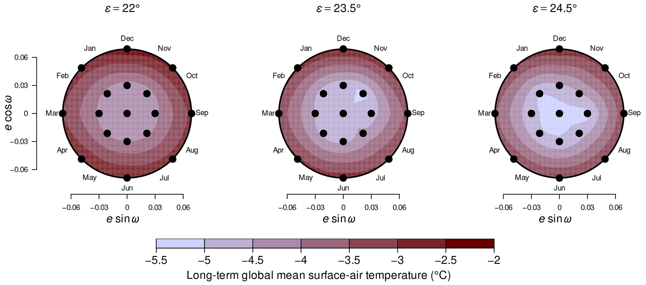
Figure 7Mean surface-air temperatures for different combinations of orbital parameters. Temperatures are taken from the warmest attractors supported for a CO2 concentration of 150 ppm and the Sturtian L+13 palaeogeography. For each obliquity ε, the eccentricity e and argument of perihelion ω are drawn as radial and angular coordinates, respectively. Abbreviations for months clarify the time of perihelion passage. Black dots denote geometries for which model simulations exist. Values between the dots result from linear interpolation.
One can observe distinct dependencies of the surface-air temperature on ε and e. First, increasing while leaving e and ω fixed reduces the temperature by 0.11–0.81 ∘C in all 17 cases; in 14 out of 17 cases, the increase leads to further cooling of up to 0.46 ∘C (and a warming of up to 0.61 ∘C in three cases). Second, increasing e from 0→0.03 for fixed ε and ω yields a surface-air warming of up to 0.86 ∘C in 23 out of 24 cases (and a cooling of 0.20 ∘C in one case); in all cases, the increase accounts for a global surface-air warming of 1.1–2.4 ∘C. Regarding the complete parameter ranges, an increase of ε from causes a global cooling of 0.21–1.0 ∘C, while an increase of e from 0→0.069 is accompanied by a warming of 1.3–2.7 ∘C.
The isolated effects of orbital parameters on surface-air temperatures are illustrated by means of a few examples in Fig. A6. Whereas, essentially, increasing ε and e has a cooling and warming effect, respectively (left and middle panels of the figure), the isolated effect of ω is less clear. For the largest eccentricity, e=0.069, one cycle of ω covers two temperature peaks when ω is near the solstices (in December and June) and two minima when ω is near the equinoxes (in September and March). This behaviour holds for all three cases with e=0.069, but the responses to variations in ω with e=0.03 are inconsistent; we neglect the latter in the detailed discussions of the ω dependence below.
4.1.1 Obliquity
As an example, we consider the zonal differences in the surface energy balance due to changing the orbital geometry from {, e=0} to {, e=0} (Fig. 8a(i)–(v)). For example, a negative temperature difference in this diagram implies a cooling contribution upon increasing the obliquity .
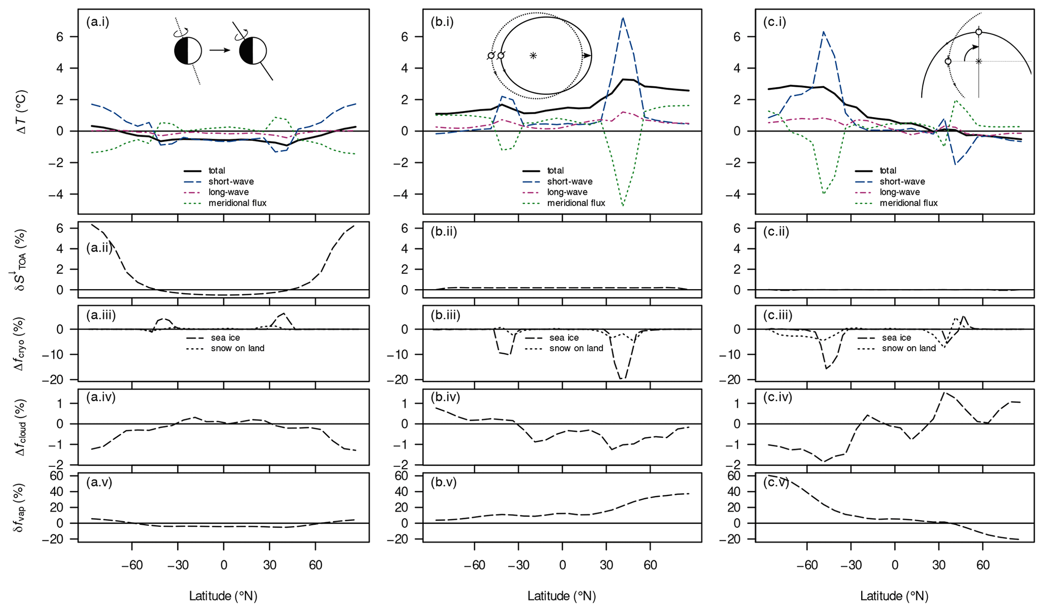
Figure 8Absolute difference in surface temperature ΔT (a(i)–c(i)), relative difference in top-of-atmosphere incoming solar flux (a(ii)–c(ii)), absolute differences in the land-snow and sea-ice fraction Δfcryo (a(iii)–c(iii)) and the cloud fraction Δfcloud (a(iv)–c(iv)), and the relative difference in column water vapour (a(v)–c(v)) between long-term-averaged attractor states upon changing individual orbital parameters. Shown in (a(i))–(c(i)) are the total temperature difference and differences due to changes in net solar radiation (“short-wave”), emissivity (“long-wave”), and meridional heat-flux divergence (“meridional flux”). Panels (a(i)–(v)) show the effects of an increased obliquity (; the reference is 22∘) with fixed e=0; panels (b(i)–(v)) show the effects of an increased eccentricity (e=0.069; the reference is 0.03) with fixed , ; and panels (c(i)–(v)) show the effects of a shifted argument of perihelion (; the reference is 180∘) with fixed , e=0.069. All differences are computed for zonal-mean magnitudes. The remaining boundary conditions are S0=1283 W m−2, a CO2 concentration of 150 ppm, and the Sturtian L+13 palaeogeography. In the inset schematics, circles depict Earth and asterisks the Sun; new configurations (the minuends) are drawn with solid lines while reference configurations (the subtrahends) are drawn with dotted lines; schematics are not to scale.
Since our obliquities are well below 55∘, the increase in ε generally yields a more evenly distributed annual-mean incoming solar flux at the top of atmosphere (e.g. Linsenmeier et al., 2015, their Fig. 2), as also seen in our example (Fig. 8a(ii)). This can explain why the change in the net solar flux causes a surface cooling around the Equator and a surface warming around the poles. The remaining features of the short-wave contribution are correlated with the differences in cryosphere fractions (Fig. 8a(iii)) and seem to illustrate processes of local ice–albedo feedback at least. This feedback can also explain minor reductions seen in the sea-ice concentration and snow cover south of around 45∘ S. Nevertheless, the global temperature differences are dominated by shifts of the cryosphere margins, which lie within the region of reduced insolation.
Changes in emissivity or heat-flux divergence mainly cause smaller differences in the surface temperature than the net solar flux. As an exception, the heat-flux divergence contributes to a cooling on the poleward sides of the cryosphere margins, exceeding the warming solar contribution. We interpret this as resulting from the decreased meridional temperature gradient in these regions: the local cooling around the cryosphere margins reduces that gradient polewards and thereby reduces the poleward heat transport there.
The local emissivity changes generally correlate well with the local balance between the short-wave and transport contributions (not shown separately, but this is evident from Fig. 8a(i)). We can attribute these changes to two positive feedbacks. First, a decrease in surface temperature lowers the atmospheric water-vapour concentration and thus raises the effective emissivity; this well-known water-vapour feedback occurs mainly in the tropics and mid-latitudes, but it also acts to enhance the high-latitude warming (Fig. 8a(v)). Second, the cooling around the cryosphere margins comes with a local decline in stratus clouds, which also increases the effective emissivity (Fig. 8a(iv)).
It is noteworthy that we observed a cooling with increased obliquity, while many studies report the opposite effect (e.g. Mantsis et al., 2011; Nowajewski et al., 2018; Brugger et al., 2019; Landwehrs et al., 2021). While those studies only investigated comparatively warm climate states with ice margins above 55∘, the cooling effect shown here is consistent with the very cold late-Carboniferous simulations of Feulner (2017). In fact, for climate states with an ice line above 55∘, our model simulates mostly rising temperatures with increased obliquity (Fig. A8).
All the discussed features are present in almost all other comparisons with differing obliquities but with other parameters fixed (not shown). There are two exceptions where increasing the obliquity from 23.5 to 24.5∘ raises the temperature (e.g. see Fig. A6), but they are not discussed in detail here.
4.1.2 Eccentricity
We investigate the effects of increased eccentricity by comparing the orbital geometries {, e=0.03, } and {, e=0.069, } (Fig. 8b(i)–(v)) corresponding to perihelion in early May. In this example, we find globally increased surface temperatures as well as a hemispheric asymmetry regarding the total temperature differences.
Changes in the net solar flux contribute almost globally to the warming. A background contribution of well below +1 ∘C can be explained by globally increased top-of-atmosphere insolation (Fig. 8b(ii)); this is due to the smaller semi-minor axis of the higher-eccentricity orbit, which results in a reduced mean Sun–Earth distance. Subannually, however, this distance oscillates, and the increased eccentricity yields a more pronounced perihelion and aphelion. For most values of ω, such as the one shown here, this increases the already existing net insolation difference between the hemispheres. This difference induces accelerated ice melting and strong warming during spring and summer in one hemisphere and delayed melting and weak relative cooling in the other. In principle, we see the same effect upon varying ω, which will be discussed below.
Outside the cryosphere margins, the warming contributions from the meridional heat-flux divergence are larger than those from the net solar flux. The local warming around the ice margins affects the meridional temperature gradients, the latter now being reduced around the Equator and enhanced over the polar ice caps. In the model, the correspondingly changing meridional heat transport causes the warming in both regions.
Changes in emissivity largely reflect the positive feedbacks already seen upon increasing the obliquity (Fig. 8b(iv)–(v)).
Depending on ω, the hemispherically asymmetric warming upon increasing the eccentricity from 0.03→0.069 can vary significantly, as discussed below. The increased global-mean insolation, however, is seen in all cases (not shown).
4.1.3 Argument of perihelion
For changes in the argument of perihelion, we look at the two orbital geometries {, e=0.069, } and {, e=0.069, } (Fig. 8c(i)–(v)), where the choices of ω represent the largest difference in surface-air temperature for a given ε and e (see Fig. A6).
Shifting ω changes neither the meridional distribution nor the annual average global amount of incoming solar flux (Fig. 8c(ii)). However, it affects the seasonal differences in insolation. At , perihelion and aphelion occur in March and September, respectively, i.e. at times with intermediate insolation in both hemispheres. In comparison, at – perihelion in December, aphelion in June – the seasonality of the solar flux is amplified in the Southern and dampened in the Northern Hemisphere. Thus, during the ice-melting seasons (spring through summer), the configuration lowers the incoming solar flux in the Northern and raises it in the Southern Hemisphere, which affects the ice-melting rates and contributes to the observed hemispheric warming–cooling asymmetry. Since the absolute increase in solar flux is larger in the Southern Hemisphere than the absolute decrease in solar flux in the Northern Hemisphere, the SH warming turns out stronger than the NH cooling. This is the main reason for the overall warming upon shifting .
Annual average short-wave reflection from snow in southern middle and high latitudes, particularly over the largest continent, is reduced at (Fig. 8c(iii)). This contributes to a significant warming at these latitudes and is a plausible reason for the configurations with being slightly warmer than those with . In order to test this hypothesis, we ran a number of simulations at varying ω with the continents mirrored at the Equator. A comparison with the original results (Fig. A9) shows that the difference between the temperature maxima at ω=90 and 270∘ can be explained by the continental configuration and, in particular, the location of the largest continent.
Changes in the meridional heat flux counteract the short-wave contributions around the ice margins and around the North Pole but play a significant role in warming the tropics and the South Pole.
Emissivity differences yield temperature changes of a smaller magnitude and the same sign as the total temperature difference, again reflecting the positive water-vapour and stratus-cloud feedbacks.
Comparing the configurations with ω=180 and 270∘, the results look very similar except for the strong warming that occurs in the Northern Hemisphere.
4.2 Equilibrium thresholds
Upon lowering the CO2 concentration to the critical levels, the sea-ice margins undergo a sudden shift from around 40∘ S/N (“Ferrel state”, Feulner et al., 2023) to the Equator for eight of the nine tested orbital geometries (Fig. A10). Only the configuration {, e=0} supports stable ice margins at around 30∘ S/N, i.e. poleward Hadley-cell boundaries (“Hadley state”, Feulner et al., 2023), before transitioning into a snowball state. The threshold for snowball inception, here defined as the highest CO2 concentration at which the transition occurs, lies between 108 ppm for {, e=0.069, } and 140 ppm for {, e=0} – a range of 30 %, relative to the lowest threshold.
A comparison of the CO2 thresholds with the surface-air temperatures at 150 ppm shows that lower temperatures favour snowball inceptions at higher CO2 concentrations (Fig. 9). One interesting exception from this rule seems to be that geometries with – perihelion in December – are more susceptible to full glaciation than those with – perihelion in June – for the same remaining boundary conditions, although the latter are generally colder than the former at 150 ppm. In fact, at CO2 concentrations close to but above the thresholds, the order is reversed and yields cooler surface-air temperatures than . Through an exemplary comparison of energy-balance contributions (Fig. A11), we identify changes in the sea-ice cover as the main reason. Well above the glaciation threshold (115 ppm and more), shifting the perihelion from June to December leaves the global sea-ice cover essentially unchanged, as hemispheric differences balance out; differences in snow cover dominate over the global temperature differences. Closer to the threshold (112 ppm), however, this shift in perihelion allows SH sea ice to form in the centre of a large subtropical gyre despite the overall SH decrease in sea-ice concentration.
Figure 9Atmospheric CO2 concentrations just above (filled circles) and below (open circles) snowball inceptions under unperturbed conditions and the corresponding long-term global mean surface-air temperatures at 150 ppm for nine different orbital geometries as indicated by the text labels.
The temperatures and thresholds presented above are the results of unperturbed simulations that took thousands of years to reach equilibrium-like states. In reality, the orbital geometry varies on a similar timescale and thus forces the climate into a permanent nonequilibrium state. Our results should therefore be understood as providing lower and upper bounds for the actual effects.
5.1 Single global volcanic perturbations
Figure 10 shows how the CO2 thresholds below which the climate enters a snowball attractor shift due to single global volcanic perturbations. Besides the trivial observation that these shifts tend to increase for stronger perturbations, we see that the results vary significantly depending on the orbital geometry. For example, a monotone and somewhat linear increase is seen for the configurations {, e=0} and {, e=0.069, }. Initialising the simulations on the coldest partially ice-covered attractors, the strongest nominal volcanic peak forcing of −40 W m−2 yields CO2-threshold shifts of up to 27 % or 40 %, respectively. (Note that all shifts in CO2 concentration are reported as percentage changes relative to the reference concentration in ppm.) However, strong perturbations initialised on the warmest partially ice-covered attractor of the former orbital configuration are much less effective, with a maximum shift of 11 %, while the initial attractor plays almost no role in the latter configuration. Strikingly, even the most extreme perturbations are barely able to trigger a snowball inception in the configuration {, e=0}. Let us now briefly investigate why, first, the initial state can make such a large difference in one orbital geometry () and, second, another orbital geometry () can show such strong resilience against perturbations.
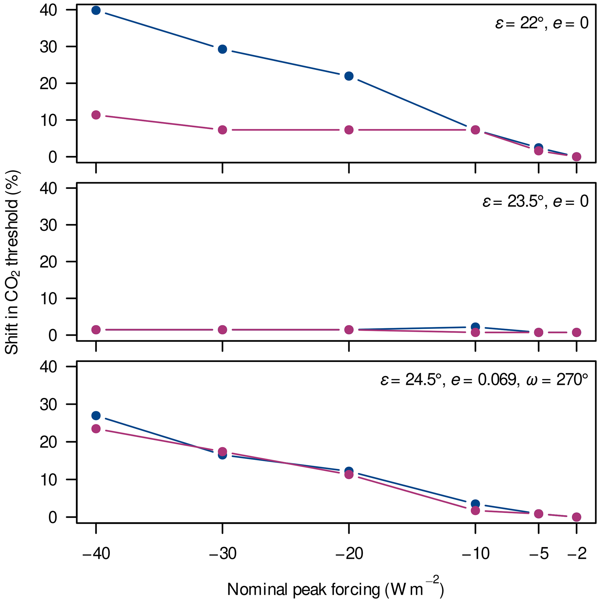
Figure 10Shift in the CO2 threshold due to single global volcanic perturbations in three different orbital configurations, each indicated within the panels. Perturbations were initialised either on the warmest (red) or on the coldest (blue) partially ice-covered attractor simulated at the respective CO2 level. For example, a shift of 10 % means that a perturbation triggers a snowball inception at a CO2 concentration 10 % above the one expected from unperturbed simulations.
In the theory of dynamical systems, a perturbation can only shift a system to a new attractor if the system is forced to cross a state separating the two basins of attraction. Consequently, differences in the response to single perturbations should be related to differences in the topology of the attractors. In Fig. 11, we plot an approximate picture permitting conclusions to be drawn about the attractors and their basins of attraction in the three different orbital configurations. Attractors were sampled by comprehensive sets of unperturbed hysteresis experiments with CO2 concentrations between 175 or 150 ppm and the respective snowball thresholds and projected onto the phase space spanned by the CO2 concentration and the global-mean surface-air temperature. The temperatures were obtained by the same procedure as used to find the thresholds for different orbital geometries (described in Sect. 2.2.2), but attractors coexisting with the warmest branches were reconstructed by incrementally increasing the CO2 concentration starting from selected states. This procedure is similar to the reconstruction of stable branches described in Brunetti and Ragon (2023) (their Method II), but an important difference is that we might (accidentally) miss “hidden” attractors that are not accessible by merely changing the boundary conditions. However, since we always allow 1000 years or more for model relaxation, the reconstructed attractors should be very precise compared to those obtained by other methods (Brunetti and Ragon, 2023).
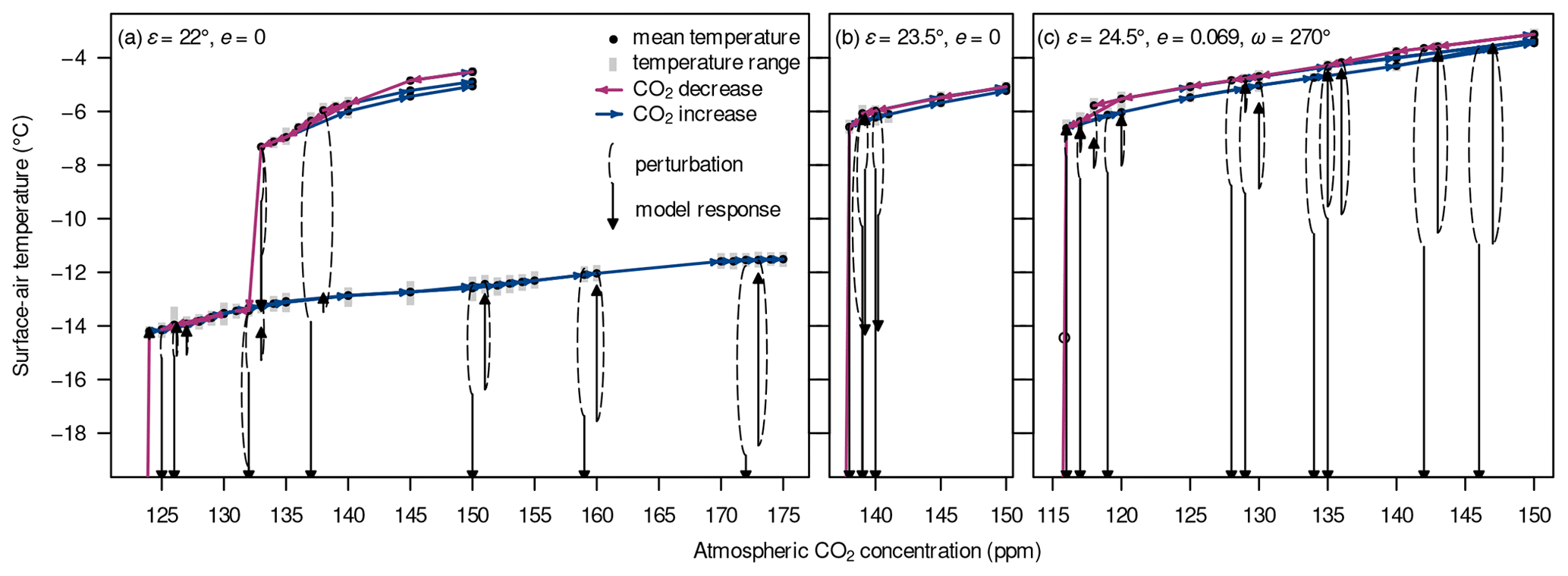
Figure 11Long-term global mean surface-air temperatures (filled circles) and temperature ranges (grey) at different CO2 concentrations in hysteresis experiments (red and blue arrows) supplemented with selected global volcanic eruptions (dashed black curves) and the model response following the peak forcing (black arrows) for the orbital geometries {, e=0} (a), {, e=0} (b), and {, e=0.069, } (c). Arrows pointing beyond the lower panel boundaries indicate transitions to snowball attractors with surface-air temperatures of around C. The open circle in panel (c) indicates that the simulation was discontinued at this temperature due to numerical instability in the course of a snowball inception.
The temperatures shown in the figure result from the annual means averaged over the last 200–1000 years of the respective simulations. Selected perturbations are shown together with the respective long-term model response in order to delineate the basins of attraction. However, it should be noted that the model typically relaxes over several hundreds of years, and the surface temperature can show an “overshooting” behaviour where further cooling after the peak forcing and subsequent relaxation to a warmer state are observed. The basins of attraction cannot therefore be inferred from the peak forcing alone.
As previously mentioned for the ice-line latitudes (Fig. A10), the configuration {, e=0} supports an intermediate cold attractor which – judging from the hysteresis experiments – seems to be absent for the other two orbital geometries. The intermediate attractor consists of “Hadley states” (Feulner et al., 2023), i.e. sea-ice margins lying at the poleward Hadley-cell boundaries, whereas the common stable states have ice margins at around 40∘ S/N and are referred to as “Ferrel states”. This dichotomy explains the strong dependence of the results on the initial conditions in the former orbital geometry. We observe that some volcanic eruptions in the configuration {, e=0} force the model into similar stable Hadley states, preventing the model from reaching a snowball inception and thereby rendering this configuration very resilient against perturbations. However, these intermediate stable states do not seem to be accessible by the quasi-static hysteresis experiments.
5.2 Single zonal volcanic perturbations
For the orbital geometry {, e=0}, Fig. 12 shows that the zonal perturbations are often comparable to the global perturbations regarding their effect on the CO2 threshold, but this effect can vary with the latitude of the eruption. The latitude dependence tends to be stronger for the larger perturbations and is especially pronounced for eruptions with a nominal peak forcing of −10 W m−2 or beyond when perturbing equilibrium states on the coldest partially ice-covered attractor. At these magnitudes, eruptions have the largest effect and mostly exceed the effects of comparable global perturbations if they occur close to the Equator. For example, an eruption with a nominal peak forcing of −20 W m−2, initialised on the colder attractor causes a shift of 24 % when centred at 15∘ N and 5 % when centred at 58∘ N; in comparison, the global perturbation shifts the threshold by 22 %. Note that there are no simulations with peak forcings of −30 or −40 W m−2 for eruptions at 58∘ S/N since the corresponding AOD values would yield a locally negative insolation using the assumed proportionality between AOD and reduction in the solar constant.
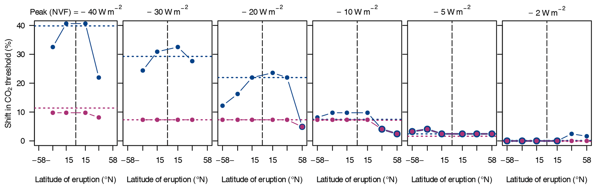
Figure 12Shifts in the CO2 threshold due to single zonal volcanic perturbations in the orbital configuration {, e=0}. Different panels contain the responses to different magnitudes of the nominal peak forcing, as indicated above each panel. Perturbations were initialised either on the warmest (red) or the coldest (blue) partially ice-covered attractor simulated at the respective CO2 level. Dotted lines indicate shifts due to global perturbations of the same magnitude.
The mechanism responsible for this latitude dependence becomes clearer upon looking at the time-dependent responses of the surface-air temperature following eruptions of the same magnitude but at different latitudes (Fig. A12). In the example shown, at 150 ppm, an eruption at 15∘ S triggers a snowball inception while an eruption at 58∘ S does not. The evolution of the surface-air temperature following the tropical eruption is very similar to the response following the global perturbation (Fig. A12, middle and top rows, respectively): in both cases we find a transient relaxation after the peak forcing but a longer-term cooling, eventually leading to a snowball Earth. More strikingly, both perturbations lead to rather homogeneous temperature reductions in the first years. The similarities come as no surprise, since our tropical eruption scenarios feature a fast spread of aerosols across all latitudes (Fig. A1). In comparison, the eruptions at higher latitudes only cause hemispherical reductions in the solar flux. The seasonal evolution of surface-air temperature shows a pattern: during the first years with high aerosol concentrations, the cooling is stronger in the respective summer hemisphere; however, for the simulations transitioning into a snowball state, the longer-term cooling happens faster in the respective winter hemisphere. This is plausible since the initial cooling results from a direct reduction in incoming radiation which is greater in absolute value for higher levels of insolation, whereas the long-term cooling comes from the more effective formation of ice during winter. For the eruptions at higher latitudes, aerosols become less dispersed over the globe and thus lead to a stronger hemispheric response (e.g. Fig. A12, bottom row). Still, the cooling leaves the tropical ocean ice-free and therefore cannot trigger a snowball inception.
The impact of the seasonal timing of an eruption cannot be thoroughly investigated with our simulations, but we observe that high-latitude events in the Northern Hemisphere often yield stronger temperature reductions (not shown) and threshold shifts (Fig. A12) than in the Southern Hemisphere. Whether this is due to the eruptions starting in January or to continental asymmetry is difficult to determine here.
5.3 Sequences of global volcanic perturbations
The different scenarios of sequential volcanic eruptions with a globally homogeneous forcing are able to produce a wide range of shifts in the CO2 threshold for a snowball inception: between 14 % and 42 %–46 % (Fig. 13). The reference scenario with parameters {p=0.1, β=1, ξ=0.3, W m−2} triggers a tipping 22 %–25 % above the equilibrium threshold in the selected orbital configuration. The smallest shift is realised by a scenario with a lower shape parameter (β=0.5), while the largest shift is observed for an increased eruption probability (p=0.3).
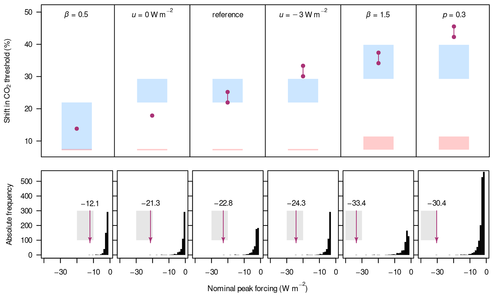
Figure 13Shifts in the CO2 threshold for snowball inception (red dots) for different scenarios of sequential volcanic eruptions (top row). The scenario is specified at the top of each panel by indicating which parameter was changed in comparison to the reference scenario {p=0.1, β=1, ξ=0.3, W m−2}. Histograms (bottom row) show the absolute frequency of eruptions with nominal peak forcings in bins of 1 W m−2. Red arrows point to the largest eruptions, with the peak forcings specified above the arrows. Blue and red rectangles indicate the expected ranges based on the effects of single global eruptions just below and above the largest events in the sequences; the corresponding ranges in the histograms are shown in grey. For the entire figure, blue colours signify perturbations on the coldest of the coexisting attractors, and red colours signify perturbations on the warmest attractors.
The top-row panels of Fig. 13 provide comparisons with the expected ranges from single global volcanic perturbations initialised on the coldest (blue rectangles) and the warmest (red) attractors coexisting at given CO2 concentrations. For example, the expected range for the reference sequence, with a strongest peak forcing of −22.8 W m−2, is determined by the shifts from single global perturbations with peak forcings of −20 and −30 W m−2. Although the sequential perturbations are initialised on the warmest attractors, all scenarios lie well above the expected ranges shown in red. Instead, five out of six cases are within or above the ranges of single perturbations acting upon the coldest equilibrium states. The reason for this is that, as mentioned before, the sequences tend to render the warmer attractors unstable and nudge the model towards the coldest ice-covered states.
Let us now investigate the differing effects of the scenarios by looking at the strongest eruptions in the time series, marked by red arrows in Fig. 13. Ignoring the last scenario (p=0.3) for a moment, the impact strictly increases with the magnitude of the largest event, which is mostly affected by the shape parameter β (−12.1 W m−2 for β=0.5; −33.4 W m−2 for β=1.5). We can distinguish three cases. First, the scenario with a threshold of u=0 W m−2 falls between the red and blue ranges. The reason is that, in the respective simulation ending in a snowball state, the largest eruption occurs while the climate is still on the warmest attractor (not shown); on the intermediate coldest attractor, the eruptions stay weaker than −17.4 W m−2 and, in fact, produce a result well between the single perturbations of −10 and −20 W m−2 (shown by the blue rectangle for the scenario β=0.5). Second, three scenarios stay within the ranges from single perturbations. For these, the effect of a sequential forcing is at least partly dominated by the single largest eruption.
Third, two scenarios, although staying below the magnitudes of certain single eruptions, have impacts that go beyond those single events. As this cannot be explained by the largest eruptions alone, the superposition of eruptions must play a role. Causing a permanent presence of aerosols from the frequent smaller eruptions, the superposition lowers the long-term temperature in almost all simulations. In the two cases of interest, the most frequent eruptions are stronger ( W m−2, see Fig. 3b) or even more frequent (p=0.3) as compared to the reference scenario, yielding an enhanced long-term cooling (not shown). This seems to amplify the sensitivity to large eruptions considerably.
It is worth noting that a recent study investigated noise-induced tipping towards snowball states in an energy-balance model under different noise types (Lucarini et al., 2022). For noise characterised by probability distributions with long tails, allowing for extreme events such as volcanic eruptions, the shape of the noise was found to be much less important for the tipping behaviour than single extreme events that trigger the tipping. Our results, obtained by prescribing noise-like volcanism, provide evidence along similar lines but additionally highlight the role of a one-sided low-magnitude noise in changing the long-term surface temperature. The major difference is the symmetry of the noise: our highly asymmetric variability in the temperature signal – roughly symmetric internal variability overlaid by one-sided volcanism – stems from the focus on volcanism and ignores some other global-scale extreme events, including those resulting from internal climate dynamics. On the other hand, it might be interesting to systematically investigate the effect of asymmetric noise in simple models.
Although the tested scenarios are based on the analysis of historical data by Ammann and Naveau (2010), it is unclear whether they are representative of the volcanic modes during the Cryogenian snowball-Earth episodes. The limited length of the applied forcing (5000 years) affects the statistics of extreme eruptions as well. Even longer model runs or ensembles, i.e. multiple simulations with the same sets of parameters, would help in assessing the thresholds more thoroughly. Nevertheless, our simulations are readily comparable with each other because they are based on the same pseudorandom time series (Fig. 3); thus, we expect the systematic effects discussed above to be robust.
One should be cautious in taking the CO2 thresholds literally, but they provide an estimate of the effects which one should expect from permanent volcanism – ranging from an impact comparable to minor changes in the continental configuration and orbital geometry up to larger shifts than those induced by the most extreme orbital configurations.
Quantifying the threshold beyond which Earth falls into a fully ice-covered state is an important prerequisite for understanding the causes of the global (or near-global) glaciations during the Neoproterozoic. Typically, this threshold is investigated in terms of critical values of the solar constant and/or the atmospheric CO2 concentration. Here, we study the influences of the continental configuration, Earth's orbital parameters, and perturbations from volcanic eruptions on the threshold for global glaciation. In the following, we briefly summarise our main findings.
Palaeogeography can have a significant influence on the snowball-inception threshold. The difference in threshold is most pronounced for the two idealised continental configurations tested here: a widely dispersed distribution and a supercontinent centred at the South Pole. While the dispersed configuration is rather susceptible to global glaciation (with an equilibrium threshold between 190 and 250 ppm of CO2, depending on the solar constant), the polar-supercontinent configuration proves to be intriguingly resistant (10–40 ppm). The thresholds of the two palaeogeographic reconstructions lie in between these extreme cases (90–180 ppm, depending on the solar constant) and differ by 6 %–44 %, relative to the lower thresholds. The differences between the various continental configurations with respect to the snowball-inception threshold can be primarily attributed to the influence of the land–ocean distribution on absorbed solar radiation at Earth's surface, with only minor contributions from changes in the meridional heat transport and the greenhouse effect from atmospheric water vapour and clouds.
Changes in orbital parameters lead to variations in the equilibrium threshold of up to 30 % relative to the lowest threshold. These differences are thus of a similar magnitude to the differences between the two palaeocontinental reconstructions. Orbital configurations with higher obliquity and lower eccentricity are generally colder and thus more susceptible to global glaciation. The dependence on eccentricity can be understood as resulting from the lower annual-mean top-of-atmosphere insolation for less elongated orbits, while the cooling with increasing obliquity can be attributed to a shift of the sea-ice margin to lower latitudes caused by the more evenly distributed annual-mean solar flux, which is amplified by the ice–albedo feedback. In the context of many earlier modelling studies, it is noteworthy that an idealised configuration with an obliquity of 23.5∘ and a circular orbit (which is fairly close to modern orbital parameters) is rather susceptible to global glaciation.
The effects of volcanic eruptions on the snowball-inception threshold depend strongly on the orbital geometry. The differences are due to changes in the stability of attractors upon changing orbital parameters. Only very large eruptions with peak forcings of −10 W m−2 or stronger can shift the threshold by a similar amount to changes in astronomical parameters. Compared to single eruptions with a globally homogeneous forcing, latitudinally resolved scenarios show a dependence on the latitude of eruption. Tropical eruptions can have significantly larger impacts than high-latitude eruptions due to a different response of surface temperatures. Simulations forced by 5000 year long sequences of volcanism allow at least two conclusions. First, the continuous noise-like perturbations can render formerly stable states unstable by connecting the basins of attraction. Second, the largest eruption in a time series mostly dictates the threshold in a similar way to single perturbations of the same magnitude; however, their effect can be amplified beyond those of single perturbations by intense background noise from frequent volcanic eruptions.
The sensitivity of Neoproterozoic snowball inceptions is severely altered by the existence or nonexistence of an intermediate state of sea-ice extent. The phenomenon is seen throughout all three tracks of simulations (i.e. those considering the continental configuration, the orbital geometry, or volcanism): a “Hadley state” with sea-ice margins at around 30∘ in latitude may exist between the ubiquitous stable state with ice margins lying at around 40∘ (“Ferrel state”, Feulner et al., 2023) and the snowball state. The Hadley state appears as an attractor accessible by quasistatic hysteresis simulations, thereby affecting the equilibrium threshold for snowball inception, in three of our configurations: the Sturtian and Marinoan M+21 palaeogeographies with an obliquity of 23.5∘ and a circular orbit, and the Sturtian L+13 continental reconstruction with an obliquity of 22∘ and a circular orbit. Additionally, we find that such an attractor is hidden from hysteresis experiments but accessible by (volcanic) perturbations in the Sturtian L+13 configuration with an obliquity of 23.5∘ and a circular orbit. For an aquaplanet setup, Feulner et al. (2023) argue that Hadley states are stabilised by large meridional temperature differences in the presence of a sufficiently high solar luminosity.
Despite the use of an oceanic general circulation model and a sea-ice scheme that captures the dynamics, our model setup comes with limitations, three of which seem to be especially relevant for snowball inceptions. First, the simplified atmosphere does not allow for changes in the Hadley-cell width, which is known to decrease under cold conditions (Frierson et al., 2007; Voigt et al., 2011), and might miscalculate the radiative transfer at low CO2 concentrations. The properties of the observed coexisting Ferrel and Hadley attractors as well as the thresholds may be affected by these limitations. Nevertheless, we expect neither the attractors to be complete artifacts nor the thresholds to be highly erroneous, as there is evidence for similar stable states in more comprehensive models (Yang et al., 2012a, b, c), and the observed thresholds lie well within the ranges determined with atmosphere–ocean general circulation models (Feulner et al., 2023). Second, we do not include ice sheets. This means that we neglect the dynamics of moving ice, which may affect the critical conditions for full glaciation under equilibrium conditions (Hyde et al., 2000) and might introduce a bias into the surface albedo. Furthermore, the absence of land ice may alter the timescales of relaxation after perturbations. However, our perturbations act on a timescale of years, which is too fast for significant changes in the land-ice extent. Third, we neglect effects of dust and volcanic ash, both of which may drastically change the snow albedo (e.g. Abbot and Pierrehumbert, 2010; Abbot and Halevy, 2010; Le Hir et al., 2010) and thus the snowball-inception threshold (Liu et al., 2021). In particular, the mitigating effect of ash during and after volcanic perturbations in a very cold climate requires further investigation.
In summary, we have shown that the distribution of continents, Earth's orbital parameters, and large volcanic eruptions can significantly shift the snowball-inception threshold under Neoproterozoic boundary conditions. In terms of the orbital geometry, the parameter values representative of the modern situation and frequently used in modelling studies turn out to be among the more susceptible configurations with respect to global glaciation, indicating a potentially greater stability of the Neoproterozoic Earth system, at least when looking at the long-term average. On the other hand, large volcanic eruptions are an inevitable contributor to natural climate variability and can shift the glaciation threshold to higher CO2 concentrations, implying that atmospheric CO2 levels might not have had to sink as low as indicated by simulations ignoring their influence. In any case, it is crucial to take these factors of natural climate variability into account in order to understand the global glaciations found in the geologic record.
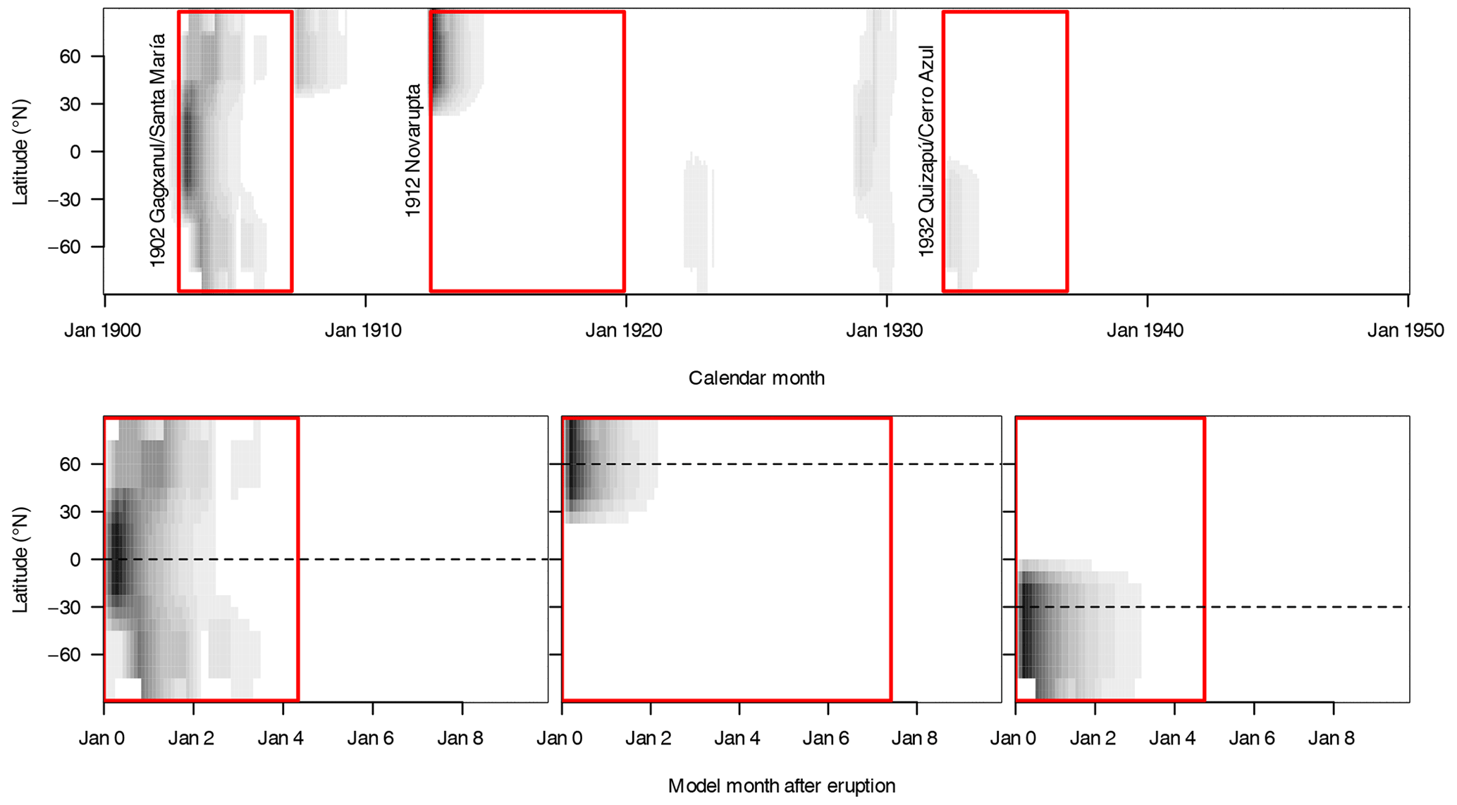
Figure A1Scenarios of monthly and zonally resolved aerosol optical depth (AOD) following historical eruptions at 15∘ N, 58∘ N, and 36∘ S. The top panel shows the part of the original data (Ammann et al., 2003) containing the selected eruptions; the bottom panels show the first 10 years of the spatially interpolated and temporally extended scenarios as used in the present study. Grey shading is proportional to AOD, but the correspondence between shading and AOD values differs between the panels.
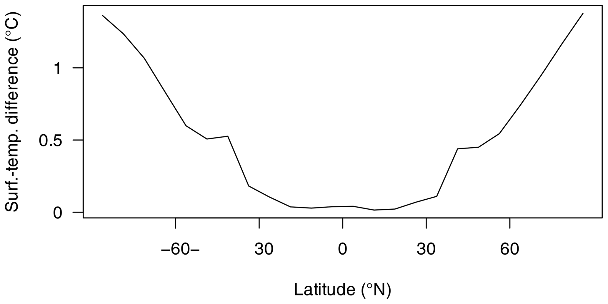
Figure A2Difference in zonal-mean surface temperature between the estimation (Eq. 2) and the actual model output from the Sturtian simulation with L+13 palaeogeography, a CO2 concentration of 250 ppm, and an orbital geometry of {, e=0}.
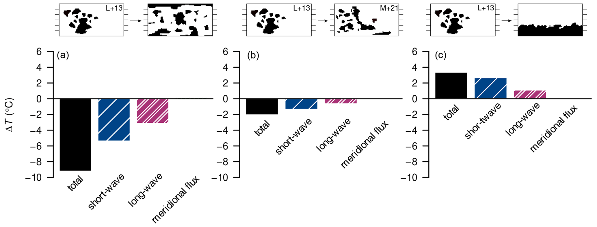
Figure A3Globally averaged surface-temperature differences and contributions from net solar radiation (“short-wave”), emissivity (“long-wave”), and meridional heat-flux divergence (“meridional flux”) for comparisons between the Sturtian L+13 continental configuration and the dispersed (a), Sturtian M+21 (b), and polar-supercontinent (c) configurations with the solar constant at 720 Ma.
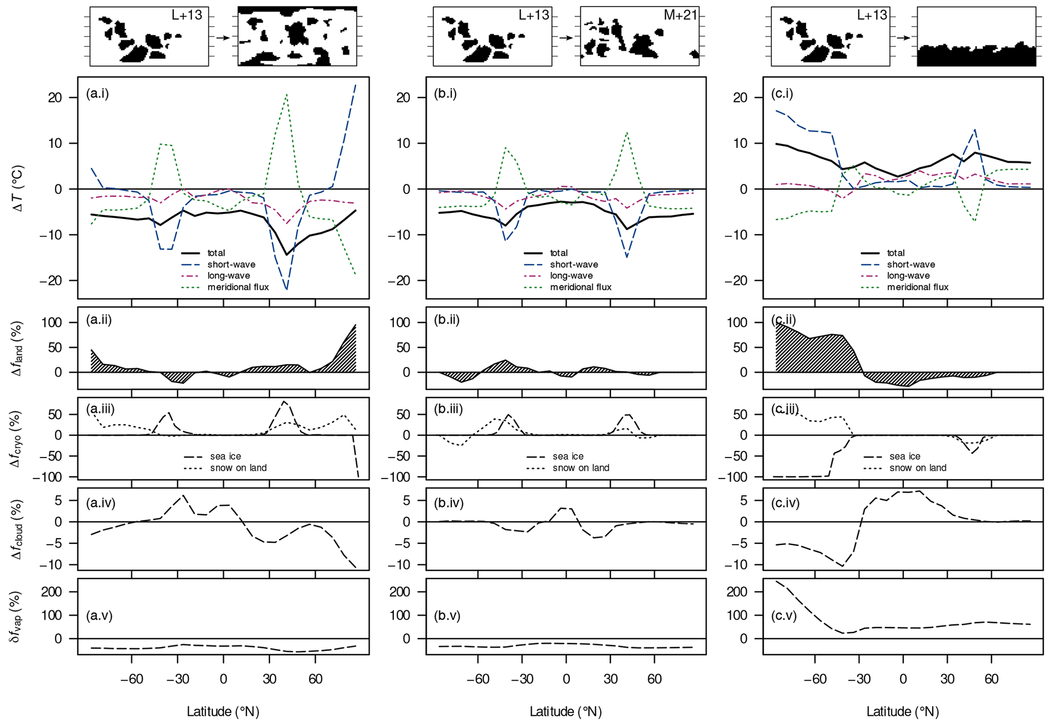
Figure A4Absolute differences in surface temperature ΔT (a(i)–c(i)), land fraction Δfland (a(ii)–c(ii)), land-snow and sea-ice fraction Δfcryo (a(iii)–c(iii)), and cloud fraction Δfcloud (a(iv)–c(iv)) and the relative difference in column water vapour (a(v)–c(v)) between long-term-averaged attractor states upon changing the continental configuration for the Marinoan onset. Shown in panels (a(i))–(c(i)) are the total temperature difference and differences due to changes in net solar radiation (“short-wave”), emissivity (“long-wave”), and meridional heat-flux divergence (“meridional flux”). Differences are computed by subtracting the values of the Marinoan L+13 reconstruction from the values of the dispersed (a(i)–(v)), the Marinoan M+21 (b(i)–(v)), or the supercontinent (c(i)–(v)) configuration. The solar constant is always 1290 W m−2 (650 Ma) and the CO2 concentration is always 200 ppm.
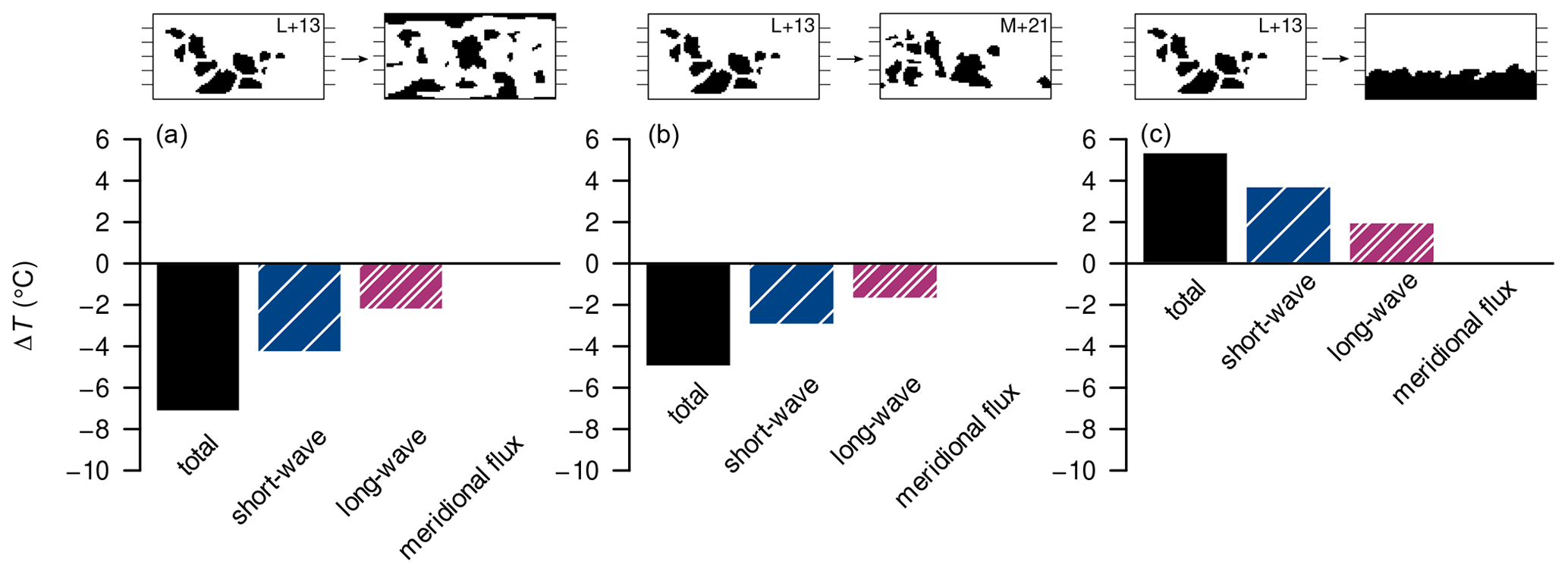
Figure A5Globally averaged surface-temperature differences and contributions from net solar radiation (“short-wave”), emissivity (“long-wave”), and meridional heat-flux divergence (“meridional flux”) for comparisons between the Marinoan L+13 continental configuration and the dispersed (a), Marinoan M+21 (b), and polar-supercontinent (c) configurations with the solar constant at 650 Ma.
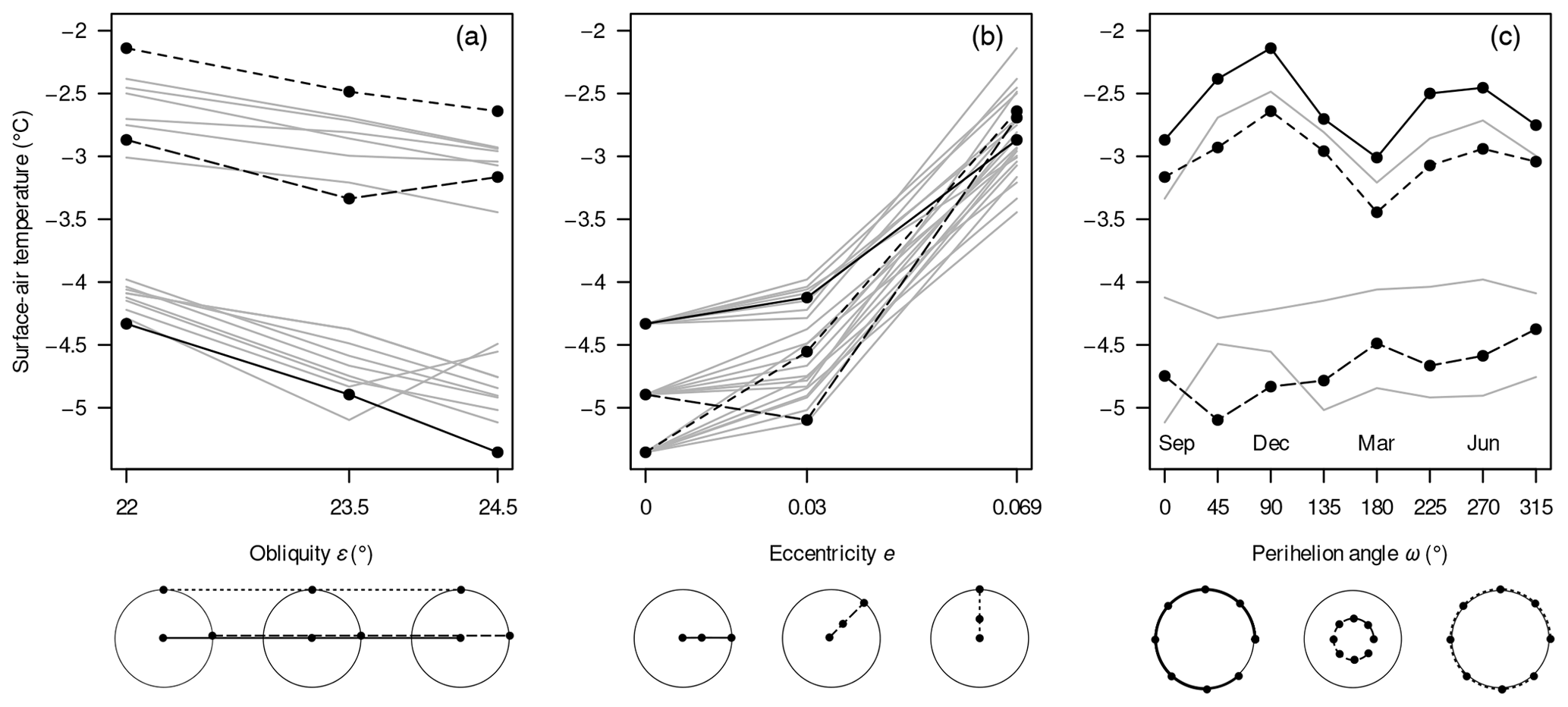
Figure A6Isolated effects of varying the orbital parameters obliquity (ε, a), eccentricity (e, b), and perihelion angle (ω, c) on the long-term global mean surface-air temperature, obtained using the data shown in Fig. 7. Below the diagrams, the selected “transects” (black curves) in parameter space are shown by reference to the polar plots in Fig. 7. All remaining curves are drawn in grey.
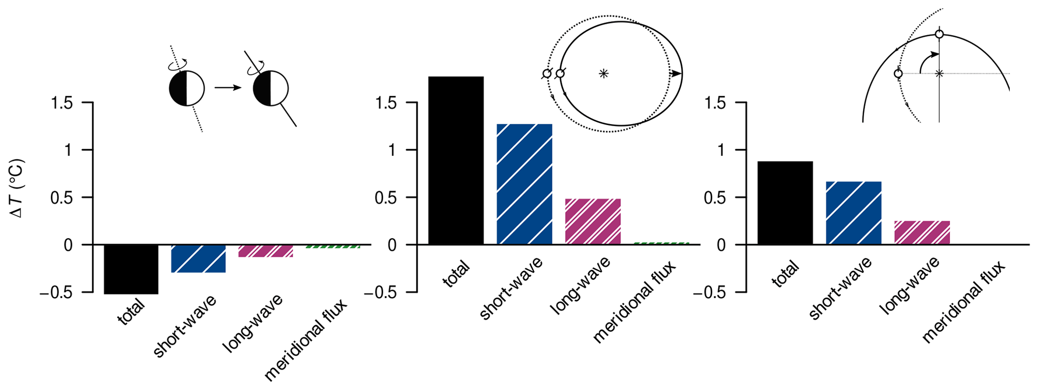
Figure A7Globally averaged surface-temperature differences and contributions from net solar radiation (“short-wave”), emissivity (“long-wave”), and meridional heat-flux divergence (“meridional flux”).
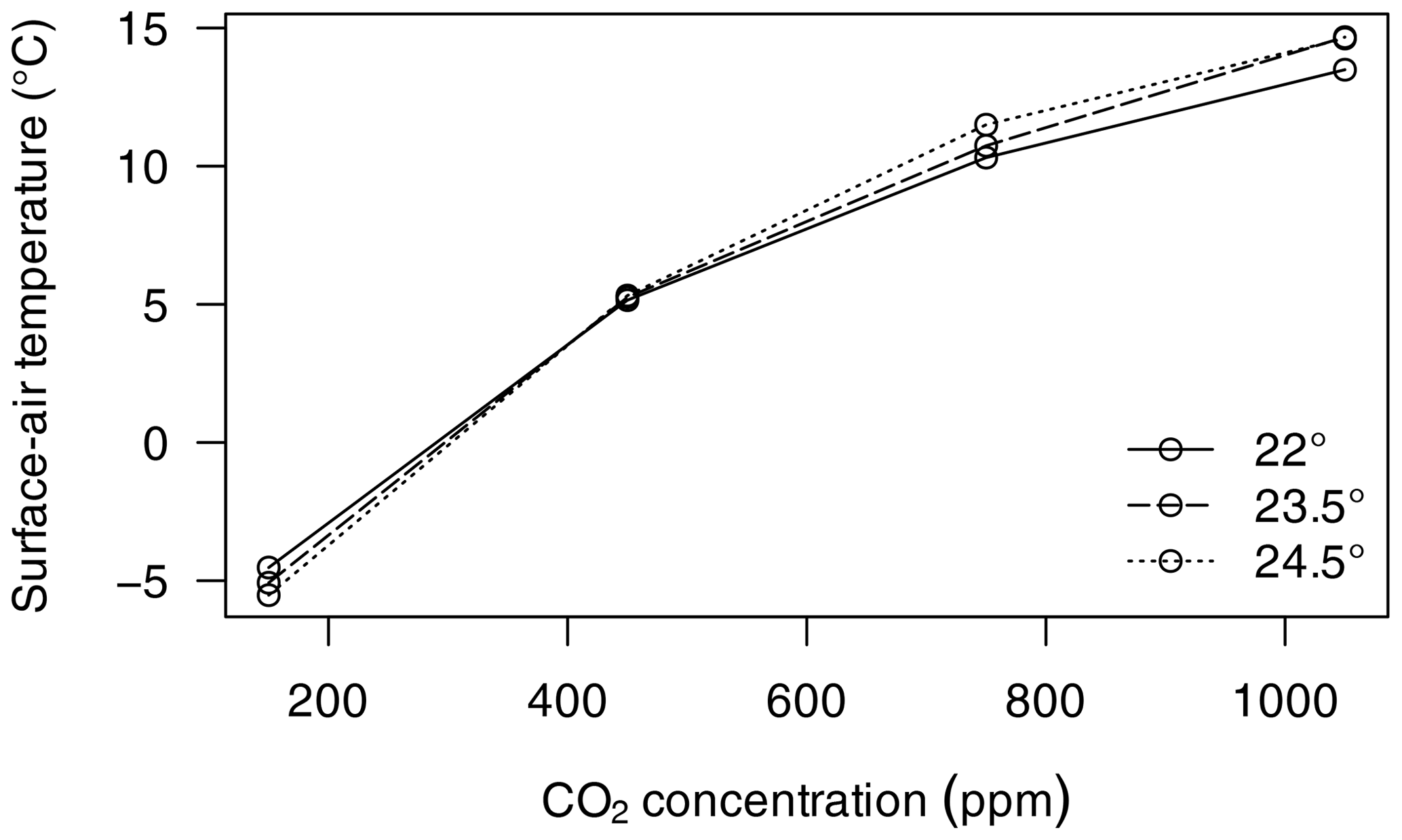
Figure A8Long-term global mean surface-air temperatures for various obliquities at different CO2 concentrations.
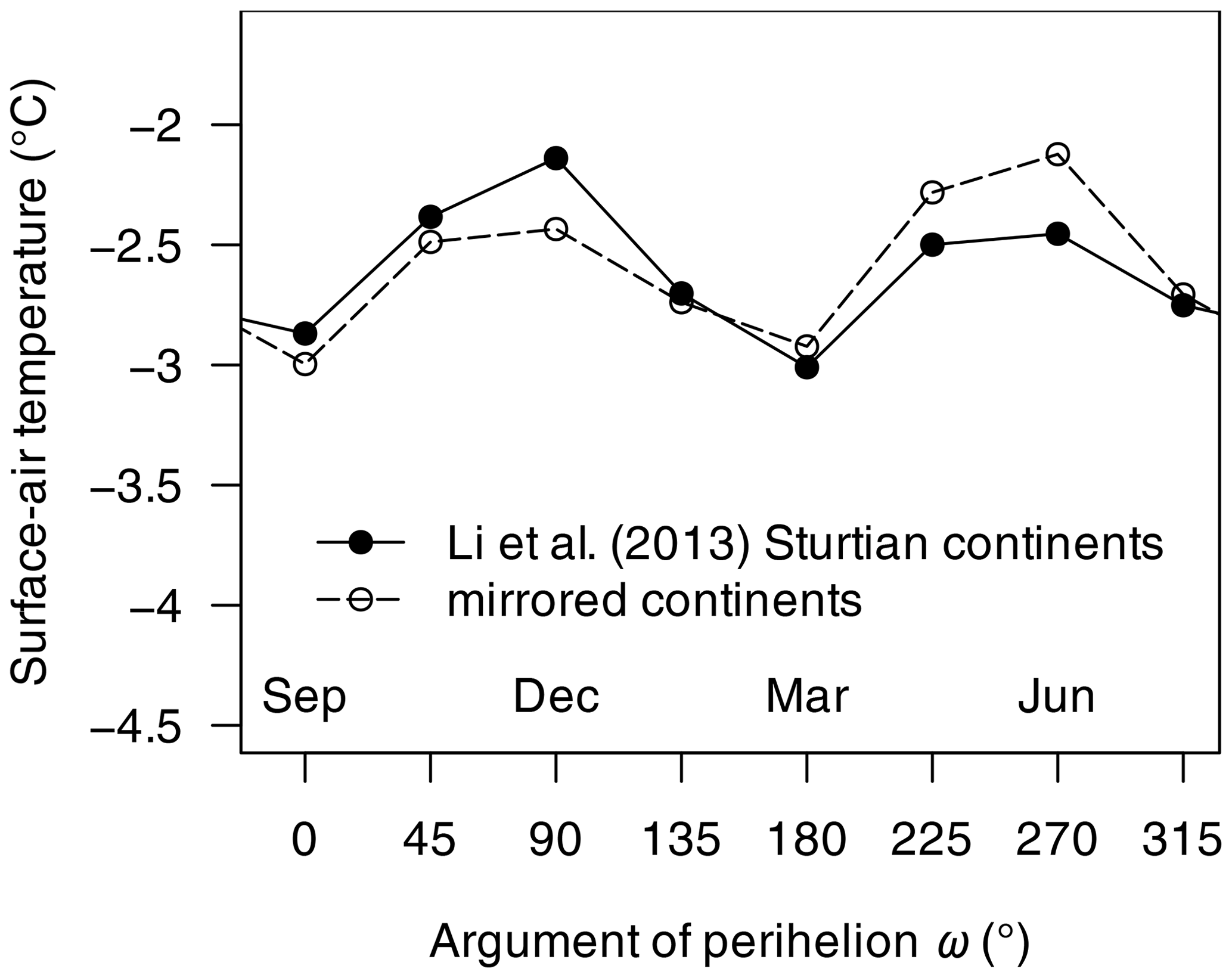
Figure A9Long-term global mean surface-air temperatures for various arguments of perihelion ω, as obtained for the Sturtian L+13 palaeogeography and for the same configuration but with the continents mirrored at the Equator.
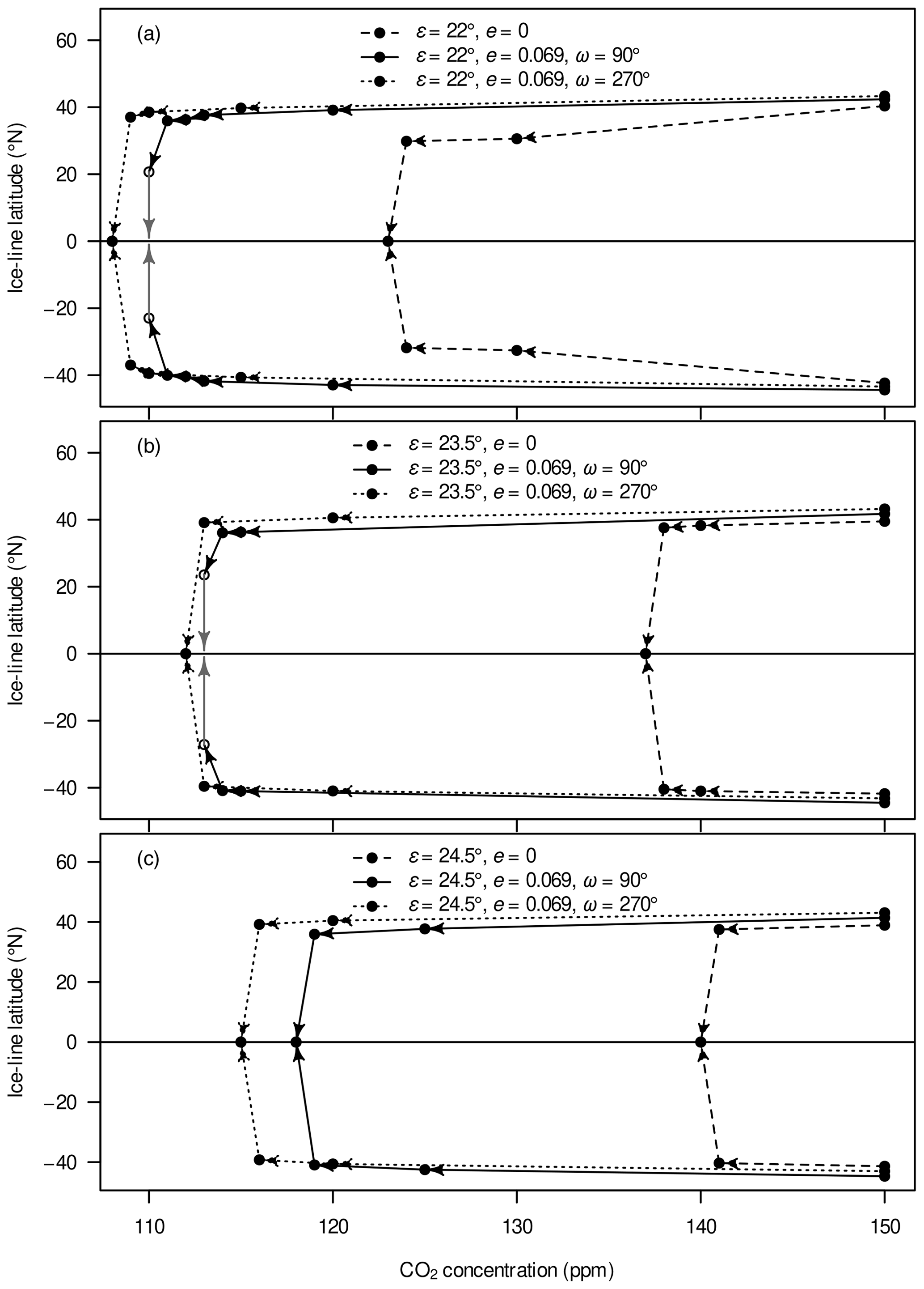
Figure A10Long-term mean ice-line latitudes, i.e. latitudes where the sea-ice concentration is 0.5, for the warmest attractors at different CO2 concentrations between 150 ppm and the respective thresholds for nine different orbital geometries with (a), 23.5∘ (b), and 24.5∘ (c).
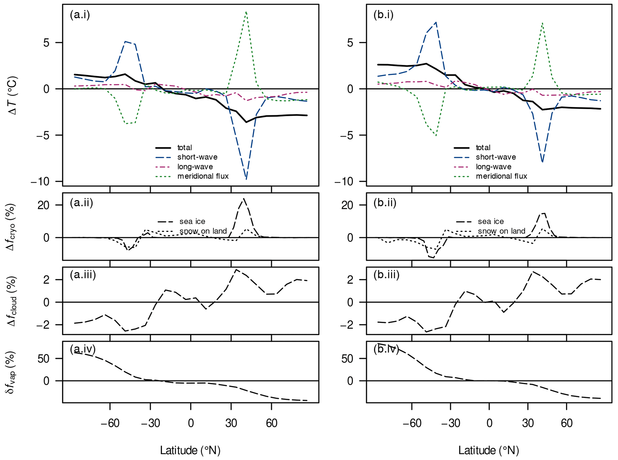
Figure A11Absolute differences in surface temperature ΔT (a(i), b(i)), land fraction Δfland (a(ii), b(ii)), land-snow and sea-ice fraction Δfcryo (a(iii), b(iii)), and cloud fraction Δfcloud (a(iv), b(iv)) and the relative difference in column water vapour (a(v), b(v)) between long-term-averaged attractor states upon shifting the argument of perihelion from for CO2 concentrations of 115 ppm (a(i)–(v)) and 112 ppm (b(i)–(v)). Other orbital parameters are , e=0.069.
Figure A12Annual (a, d, g), December–January–February (DJF, middle column), and June–July–August (JJA, c, f, i) mean zonal differences in surface-air temperature in selected years following volcanic eruptions with a nominal peak forcing of −20 W m−2. Eruptions are applied as either globally homogeneous perturbations (a–c), zonal perturbations centred around 15∘ S (d–f), or zonal perturbations centred around 58∘ S (g–i). Differences are computed with respect to the last year before the eruption. Small arrows indicate the latitudes of eruption.
Table B1Long-term global mean surface-air temperatures for different combinations of the orbital parameters obliquity (ε), eccentricity (e), and argument of perihelion (ω). Note that for e=0, ω is not well defined.
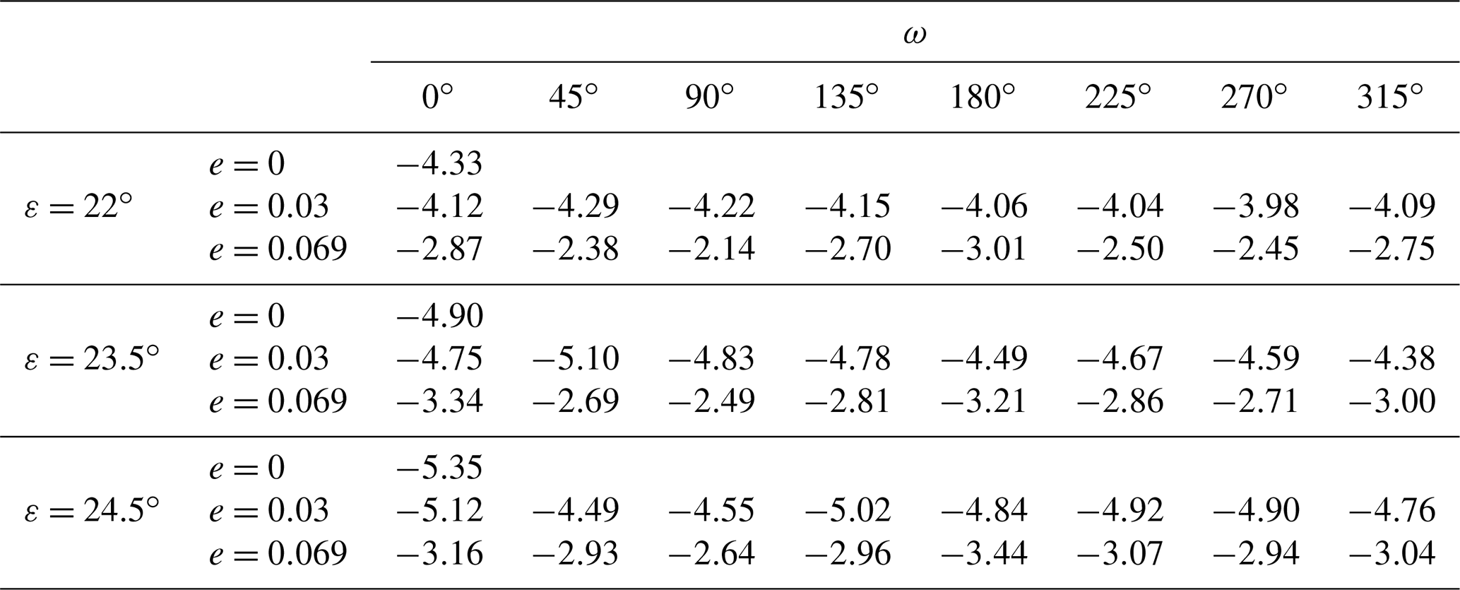
Model input and output files as well as the scripts used to generate the figures are available at the institutional repository of the Potsdam Institute for Climate Impact Research (Eberhard et al., 2023, https://doi.org/10.5880/PIK.2023.002). The model source code will be made available upon request.
JE, OEB, and GF designed the study; OEB and GF prepared the continental boundary-condition data with input from JvH and JULB; OEB performed and analysed the model simulations on continental configurations with input from JE and GF; JE performed and analysed the model simulations on orbital geometry and volcanism with input from GF; SP provided technical assistance and compiled the data archive; JE prepared the figures; JE, OEB, and GF wrote the paper with input from all co-authors.
The contact author has declared that none of the authors has any competing interests.
Publisher’s note: Copernicus Publications remains neutral with regard to jurisdictional claims in published maps and institutional affiliations.
The authors gratefully acknowledge the European Regional Development Fund (ERDF), the German Federal Ministry of Education and Research and the Land Brandenburg for supporting this project by providing resources on the high-performance computer system at the Potsdam Institute for Climate Impact Research. The authors thank the referees Yonggang Liu, Dorian Abbot, and Aiko Voigt for their critique and suggestions, which significantly improved the paper.
This project received funding from the European Research Council (ERC) under the European Union’s Horizon 2020 research and innovation programme (grant agreement no. 856555).
The article processing charges for this open-access publication were covered by the Potsdam Institute for Climate Impact Research (PIK).
This paper was edited by Yannick Donnadieu and reviewed by Yonggang Liu, Aiko Voigt, and Dorian Abbot.
Abbot, D. and Halevy, I.: Dust aerosol important for Snowball Earth deglaciation, J. Climate, 23, 4121–4132, https://doi.org/10.1175/2010JCLI3378.1, 2010. a, b
Abbot, D. and Pierrehumbert, R.: Mudball: surface dust and Snowball Earth deglaciation, J. Geophys. Res., 115, D03104, https://doi.org/10.1029/2009JD012007, 2010. a, b
Abbot, D., Voigt, A., and Koll, D.: The Jormungand global climate state and implications for Neoproterozoic glaciations, J. Geophys. Res., 116, D18103, https://doi.org/10.1029/2011JD015927, 2011. a
Allen, P. and Etienne, J.: Sedimentary challenge to Snowball Earth, Nat. Geosci., 1, 817–825, https://doi.org/10.1038/ngeo355, 2008. a
Ammann, C. and Naveau, P.: A statistical volcanic forcing scenario generator for climate simulations, J. Geophys. Res., 115, D05107, https://doi.org/10.1029/2009JD012550, 2010. a, b, c, d, e, f
Ammann, C., Meehl, G., Washington, W., and Zender, C.: A monthly and latitudinally varying volcanic forcing dataset in simulations of 20th century climate, Geophys. Res. Lett., 30, 1657, https://doi.org/10.1029/2003GL016875, 2003. a, b, c
Ashwin, P., Wieczorek, S., Vitolo, R., and Cox, P.: Tipping points in open systems: bifurcation, noise-induced and rate-dependent examples in the climate system, Philos. T. R. Soc. A, 370, 1166–1184, https://doi.org/10.1098/rsta.2011.0306, 2012. a, b
Bahcall, J., Pinsonneault, M., and Basu, S.: Solar models: current epoch and time dependencies, neutrinos, and helioseismological properties, Astrophys. J., 555, 990–1012, https://doi.org/10.1086/321493, 2001. a, b
Berger, A. and Loutre, M.: Precession, eccentricity, obliquity, insolation and paleoclimates, in: Long-term climatic variations. Data and modelling, edited by: Duplessy, J.-C. and Spyridakis, M.-T., vol. 22 of NATO ASI subseries I: Global environmental change, Springer, 107–151, https://doi.org/10.1007/978-3-642-79066-9_5, 1994. a
Brady, P. and Carroll, S.: Direct effects of CO2 and temperature on silicate weathering: possible implications for climate control, Geochim. Cosmochim. Ac., 58, 1853–1856, https://doi.org/10.1016/0016-7037(94)90543-6, 1994. a
Brugger, J., Hofmann, M., Petri, S., and Feulner, G.: On the sensitivity of the Devonian climate to continental configuration, vegetation cover, orbital configuration, CO2 concentration, and insolation, Paleoceanogr. Paleoclimatol., 34, 1375–1398, https://doi.org/10.1029/2019PA003562, 2019. a
Brunetti, M. and Ragon, C.: Attractors and bifurcation diagrams in complex climate models, Phys. Rev. E, 107, 054214, https://doi.org/10.1103/PhysRevE.107.054214, 2023. a, b
Crowley, T., Zielinski, G., Vinther, B., Udisti, R., Kreutz, K., Cole-Dai, J., and Castellano, E.: Volcanism and the Little Ice Age, PAGES News, 16, 22–23, https://doi.org/10.22498/PAGES.16.2.22, 2008. a
Dalziel, I.: Overview: Neoproterozoic–Paleozoic geography and tectonics: review, hypothesis, environmental speculation, GSA Bull., 109, 16–42, https://doi.org/10.1130/0016-7606(1997)109<0016:ONPGAT>2.3.CO;2, 1997. a
Donnadieu, Y., Ramstein, G., Fluteau, F., Besse, J., and Meert, J.: Is high obliquity a plausible cause for Neoproterozoic glaciations?, Geophys. Res. Lett., 29, 2127, https://doi.org/10.1029/2002GL015902, 2002. a
Eberhard, J., Bevan, O., Feulner, G., Petri, S., van Hunen, J., and Baldini, J.: Climate model ensemble data for Neoproterozoic Snowball-Earth inceptions, GFZ Data Services [data set], https://doi.org/10.5880/PIK.2023.002, 2023. a
Embrechts, P., Klüppelberg, C., and Mikosch, T.: Modelling extremal events for insurance and finance, Springer, https://doi.org/10.1007/978-3-642-33483-2, 1997. a, b
Feulner, G.: The faint young Sun problem, Rev. Geophys., 50, RG2006, https://doi.org/10.1029/2011RG000375, 2012. a
Feulner, G.: Formation of most of our coal brought Earth close to global glaciation, P. Natl. Acad. Sci. USA, 114, 11333–11337, https://doi.org/10.1073/pnas.1712062114, 2017. a
Feulner, G. and Kienert, H.: Climate simulations of Neoproterozoic snowball Earth events: similar critical carbon dioxide levels for the Sturtian and Marinoan glaciations, Earth Planet. Sc. Lett., 404, 200–205, https://doi.org/10.1016/j.epsl.2014.08.001, 2014. a, b, c, d
Feulner, G., Hallmann, C., and Kienert, H.: Snowball cooling after algal rise, Nat. Geosci., 8, 659–662, https://doi.org/10.1038/ngeo2523, 2015. a, b
Feulner, G., Bukenberger, M., and Petri, S.: Tracing the Snowball bifurcation of aquaplanets through time reveals a fundamental shift in critical-state dynamics, Earth Syst. Dynam., 14, 533–547, https://doi.org/10.5194/esd-14-533-2023, 2023. a, b, c, d, e, f, g, h, i, j, k
Fichefet, T. and Morales Maqueda, M.: Sensitivity of a global sea ice model to the treatment of ice thermodynamics and dynamics, J. Geophys. Res., 102, 12609–12646, https://doi.org/10.1029/97JC00480, 1997. a
Frierson, D., Lu, J., and Chen, G.: Width of the Hadley cell in simple and comprehensive general circulation models, Geophys. Res. Lett., 34, L18804, https://doi.org/10.1029/2007GL031115, 2007. a
Gao, C., Robock, A., and Ammann, C.: Volcanic forcing of climate over the past 1500 years: an improved ice core-based index for climate models, J. Geophys. Res., 113, D23111, https://doi.org/10.1029/2008JD010239, 2008. a, b
Goddéris, Y., Donnadieu, Y., Nédélec, A., Dupré, B., Dessert, C., Grard, A., Ramstein, G., and François, L.: The Sturtian `snowball' glaciation: fire and ice, Earth Planet. Sc. Lett., 211, 1–12, https://doi.org/10.1016/S0012-821X(03)00197-3, 2003. a
Goode, P., Qiu, J., Yurchyshyn, V., and Hickey, J.: Earthshine observations of the Earth's reflectance, Geophys. Res. Lett., 28, 1671–1674, https://doi.org/10.1029/2000GL012580, 2001. a
Gupta, M., Marshall, J., and Ferreira, D.: Triggering global climate transitions through volcanic eruptions, J. Climate, 32, 3727–3742, https://doi.org/10.1175/JCLI-D-18-0883.1, 2019. a, b
Halekotte, L. and Feudel, U.: Minimal fatal shocks in multistable complex networks, Sci. Rep., 11783, https://doi.org/10.1038/s41598-020-68805-6, 2020. a, b
Heinemann, M., Jungclaus, J. H., and Marotzke, J.: Warm Paleocene/Eocene climate as simulated in ECHAM5/MPI-OM, Clim. Past, 5, 785–802, https://doi.org/10.5194/cp-5-785-2009, 2009. a
Held, I. and Suarez, M.: Simple albedo feedback models of the icecaps, Tellus, 26, 613–629, https://doi.org/10.3402/tellusa.v26i6.9870, 1974. a
Hoffman, P. and Schrag, D.: The snowball Earth hypothesis: testing the limits of global change, Terra Nova, 14, 129–155, https://doi.org/10.1046/j.1365-3121.2002.00408.x, 2002. a
Hoffman, P., Kaufman, A., Halverson, G., and Schrag, D.: A Neoproterozoic snowball Earth, Science, 281, 1342–1346, https://doi.org/10.1126/science.281.5381.1342, 1998. a
Hoffman, P., Abbot, D., Ashkenazy, Y., Benn, D., Brocks, J., Cohen, P., Cox, G., Creveling, J., Donnadieu, Y., Erwin, D., Fairchild, I., Ferreira, D., Goodman, J., Halverson, G., Jansen, M., Le Hir, G., Love, G., Macdonald, F., Maloof, A., Partin, C., Ramstein, G., Rose, B., Rose, C., Sadler, P., Tziperman, E., Voigt, A., and Warren, S.: Snowball Earth climate dynamics and Cryogenian geology–geobiology, Sci. Adv., 3, e1600983, https://doi.org/10.1126/sciadv.1600983, 2017. a, b, c, d, e, f, g
Hofmann, M. and Morales Maqueda, M.: Performance of a second-order moments advection scheme in an ocean general circulation model, J. Geophys. Res., 111, C05006, https://doi.org/10.1029/2005JC003279, 2006. a
Hunke, E. and Dukowicz, J.: An elastic–viscous–plastic model for sea ice dynamics, J. Phys. Oceanogr., 27, 1849–1867, https://doi.org/10.1175/1520-0485(1997)027<1849:AEVPMF>2.0.CO;2, 1997. a
Hyde, W., Crowley, T., Baum, S., and Peltier, W.: Neoproterozoic `snowball Earth' simulations with a coupled climate/ice-sheet model, Nature, 405, 425–429, https://doi.org/10.1038/35013005, 2000. a, b, c, d
Jenkins, G.: Examining the sensitivity of Earth's climate to the removal of ozone, landmasses and enhanced ocean heat transport in the GENESIS global climate model, Global Planet. Change, 20, 257–279, https://doi.org/10.1016/S0921-8181(98)00070-8, 1999. a, b
Jones, G., Gregory, J., Stott, P., Tett, S., and Thorpe, R.: An AOGCM simulation of the climate response to a volcanic super-eruption, Clim. Dynam., 25, 725–738, https://doi.org/10.1007/s00382-005-0066-8, 2005. a
Kirschvink, J.: Late Proterozoic low-latitude global glaciation: the snowball earth, in: The Proterozoic biosphere: a multidisciplinary study, edited by: Schopf, J. and Klein, C., Cambridge University Press, 51–52, https://resolver.caltech.edu/CaltechAUTHORS:20130117-100718783 (last access: 19 October 2023), 1992. a
Landwehrs, J., Feulner, G., Petri, S., Sames, B., and Wagreich, M.: Investigating Mesozoic climate trends and sensitivities with a large ensemble of climate model simulations, Paleoceanogr. Paleoclimatol., 36, 2020PA004134, https://doi.org/10.1029/2020PA004134, 2021. a
Laskar, J., Robutel, P., Joutel, F., Gastineau, M., Correia, A., and Levrard, B.: A long-term numerical solution for the insolation quantities of the Earth, Astron. Astrophys., 428, 261–285, https://doi.org/10.1051/0004-6361:20041335, 2004. a
Le Hir, G., Donnadieu, Y., Krinner, G., and Ramstein, G.: Toward the snowball earth deglaciation…, Clim. Dynam., 35, 285–297, https://doi.org/10.1007/s00382-010-0748-8, 2010. a, b
Lewis, J., Weaver, A., Johnston, S., and Eby, M.: Neoproterozoic “snowball Earth”: dynamic sea ice over a quiescent ocean, Paleoceanogr., 18, 1092, https://doi.org/10.1029/2003PA000926, 2003. a, b
Li, Z., Evans, D., and Halverson, G.: Neoproterozoic glaciations in a revised global palaeogeography from the breakup of Rodinia to the assembly of Gondwanaland, Sediment. Geol., 294, 219–232, https://doi.org/10.1016/j.sedgeo.2013.05.016, 2013. a, b, c, d, e
Linsenmeier, M., Pascale, S., and Lucarini, V.: Climate of Earth-like planets with high obliquity and eccentric orbits: implications for habitability conditions, Planet. Space Sci., 105, 43–59, https://doi.org/10.1016/j.pss.2014.11.003, 2015. a
Liu, Y., Peltier, W. R., Yang, J., and Vettoretti, G.: The initiation of Neoproterozoic ”snowball” climates in CCSM3: the influence of paleocontinental configuration, Clim. Past, 9, 2555–2577, https://doi.org/10.5194/cp-9-2555-2013, 2013. a, b, c
Liu, Y., Liu, P., Li, D., Peng, Y., and Hu, Y.: Influence of dust on the initiation of Neoproterozoic snowball Earth events, J. Climate, 34, 6673–6689, https://doi.org/10.1175/JCLI-D-20-0803.1, 2021. a
Lucarini, V. and Bódai, T.: Edge states in the climate system: exploring global instabilities and critical transitions, Nonlinearity, 30, R32–R66, https://doi.org/10.1088/1361-6544/aa6b11, 2017. a
Lucarini, V., Fraedrich, K., and Lunkeit, F.: Thermodynamic analysis of snowball Earth hysteresis experiment: efficiency, entropy production and irreversibility, Q. J. R. Meteor. Soc., 136, 2–11, https://doi.org/10.1002/qj.543, 2010. a
Lucarini, V., Serdukova, L., and Margazoglou, G.: Lévy noise versus Gaussian-noise-induced transitions in the Ghil–Sellers energy balance model, Nonlin. Processes Geophys., 29, 183–205, https://doi.org/10.5194/npg-29-183-2022, 2022. a
Macdonald, F. and Wordsworth, R.: Initiation of Snowball Earth with volcanic sulfur aerosol emissions, Geophys. Res. Lett., 44, 1938–1946, https://doi.org/10.1002/2016GL072335, 2017. a, b, c
Mantsis, D., Clement, A., Broccoli, A., and Erb, M.: Climate feedbacks in response to changes in obliquity, J. Climate, 24, 2830–2845, https://doi.org/10.1175/2010JCLI3986.1, 2011. a
Merdith, A., Collins, A., Williams, S., Pisarevsky, S., Foden, J., Archibald, D., Blades, M., Alessio, B., Armistead, S., Plavsa, D., Clark, C., and Müller, R.: A full-plate global reconstruction of the Neoproterozoic, Gondwater Res., 50, 84–134, https://doi.org/10.1016/j.gr.2017.04.001, 2017. a
Merdith, A., Williams, S., Collins, A., Tetley, M., Mulder, J., Blades, M., Young, A., Armistead, S., Cannon, J., Zahirovic, S., and Müller, R.: Extending full-plate tectonic models into deep time: linking the Neoproterozoic and the Phanerozoic, Earth-Sci. Rev., 214, 103477, https://doi.org/10.1016/j.earscirev.2020.103477, 2021. a, b, c, d, e, f, g, h
Metzner, D., Kutterolf, S., Toohey, M., Timmreck, C., Niemeier, U., Freundt, A., and Krüger, K.: Radiative forcing and climate impact resulting from SO2 injections based on a 200,000-year record of Plinian eruptions along the Central American Volcanic Arc, Int. J. Earth Sci. (Geol. Rundsch.), 103, 2063–2079, https://doi.org/10.1007/s00531-012-0814-z, 2014. a
Milanković, M.: Kanon der Erdbestrahlung und seine Anwendung auf das Eiszeitenproblem, Königlich Serbische Akademie, Belgrad, 1941.-3 a, b
Mitchell, R., Gernon, T., Cox, G., Nordsvan, A., Kirscher, U., Xuan, C., Liu, Y., and He, X.: Orbital forcing of ice sheets during snowball Earth, Nat. Commun., 12, 4187, https://doi.org/10.1038/s41467-021-24439-4, 2021. a
Moczydłowska, M.: The Ediacaran microbiota and the survival of Snowball Earth conditions, Precambrian Res., 167, 1–15, https://doi.org/10.1016/j.precamres.2008.06.008, 2008. a
Montoya, M., Griesel, A., Levermann, A., Mignot, J., Hofmann, M., Ganopolski, A., and Rahmstorf, S.: The earth system model of intermediate complexity CLIMBER-3α. Part I: description and performance for present-day conditions, Clim. Dynam., 25, 237–263, https://doi.org/10.1007/s00382-005-0044-1, 2005. a, b, c
Müller, P.: Handbook of dynamics and probability, Springer, https://doi.org/10.1007/978-3-030-88486-4, 2022. a
Müller, R., Cannon, J., Qin, X., Watson, R., Gurnis, M., Williams, S., Pfaffelmoser, T., Seton, M., Russell, S., and Zahirovic, S.: GPlates: building a virtual Earth through deep time, Geochem. Geophy. Geosy., 19, 2243–2261, https://doi.org/10.1029/2018GC007584, 2018. a
Naveau, P. and Ammann, C.: Statistical distributions of ice core sulfate from climatically relevant volcanic eruptions, Geophys. Res. Lett., 32, L05711, https://doi.org/10.1029/2004GL021732, 2005. a, b
North, G. and Kim, K.: Energy balance climate models, Wiley-VCH, Weinheim, https://doi.org/10.1002/9783527698844, 2017. a
Nowajewski, P., Rojas, M., Rojo, R., and Kimeswenger, S.: Atmospheric dynamics and habitability range in Earth-like aquaplanets obliquity simulations, Icarus, 305, 84–90, https://doi.org/10.1016/j.icarus.2018.01.002, 2018. a
Olcott, A., Sessions, A., Corsetti, F., Kaufman, A., and de Oliviera, T.: Biomarker evidence for photosynthesis during Neoproterozoic glaciation, Science, 310, 471–474, https://doi.org/10.1126/science.1115769, 2005. a
Olson, S., Jansen, M., Abbot, D., Halevy, I., and Goldblatt, C.: The effect of ocean salinity on climate and its implications for Earth's habitability, Geophys. Res. Lett., 49, e2021GL095748, https://doi.org/10.1029/2021GL095748, 2022. a
Pacanowski, R. and Griffies, S.: MOM 3.0 manual, Tech. rep., NOAA/Geophysical Fluid Dynamics Laboratory, Princeton, GitHub, https://mom-ocean.github.io/assets/pdfs/MOM3_manual.pdf (last access: 28 April 2023), 2000. a
Palter, J.: The role of the Gulf Stream in European climate, Annu. Rev. Mar. Sci., 7, 113–137, https://doi.org/10.1146/annurev-marine-010814-015656, 2015. a
Peixoto, J. and Oort, A.: Physics of Climate, Springer, New York, ISBN 978-0-88318-712-8, 1992. a
Petoukhov, V., Ganopolski, A., Brovkin, V., Claussen, M., Eliseev, A., Kubatzki, C., and Rahmstorf, S.: CLIMBER-2: a climate system model of intermediate complexity. Part I: model description and performance for present climate, Clim. Dynam., 16, 1–17, https://doi.org/10.1007/PL00007919, 2000. a, b
Pierrehumbert, R.: Principles of planetary climate, Cambridge University Press, New York, https://doi.org/10.1017/CBO9780511780783, 2010. a
Pierrehumbert, R., Abbot, D., Voigt, A., and Koll, D.: Climate of the Neoproterozoic, Annu. Rev. Earth Pl. Sc., 39, 417–460, https://doi.org/10.1146/annurev-earth-040809-152447, 2011. a, b
Ridgwell, A., Kennedy, M., and Caldeira, K.: Carbonate deposition, climate stability, and Neoproterozoic ice ages, Science, 302, 859–862, https://doi.org/10.1126/science.1088342, 2003. a
Robock, A.: Volcanic eruptions and climate, Rev. Geophys., 38, 191–219, https://doi.org/10.1029/1998RG000054, 2000. a
Robock, A., Ammann, C., Oman, L., Shindell, D., Levis, S., and Stenchikov, G.: Did the Toba volcanic eruption of ∼ 74 ka B.P. produce widespread glaciation?, J. Geophys. Res.-Atmos., 114, D10107, https://doi.org/10.1029/2008JD011652, 2009. a
Roe, G. and Baker, M.: Notes on a catastrophe: a feedback analysis of snowball Earth, J. Climate, 23, 4694–4703, https://doi.org/10.1175/2010JCLI3545.1, 2010. a
Schmidt, G. A., Jungclaus, J. H., Ammann, C. M., Bard, E., Braconnot, P., Crowley, T. J., Delaygue, G., Joos, F., Krivova, N. A., Muscheler, R., Otto-Bliesner, B. L., Pongratz, J., Shindell, D. T., Solanki, S. K., Steinhilber, F., and Vieira, L. E. A.: Climate forcing reconstructions for use in PMIP simulations of the Last Millennium (v1.1), Geosci. Model Dev., 5, 185–191, https://doi.org/10.5194/gmd-5-185-2012, 2012. a
Segschneider, J., Beitsch, A., Timmreck, C., Brovkin, V., Ilyina, T., Jungclaus, J., Lorenz, S. J., Six, K. D., and Zanchettin, D.: Impact of an extremely large magnitude volcanic eruption on the global climate and carbon cycle estimated from ensemble Earth System Model simulations, Biogeosciences, 10, 669–687, https://doi.org/10.5194/bg-10-669-2013, 2013. a
Timmreck, C., Graf, H.-F., Lorenz, S., Niemeier, U., Zanchettin, D., Matei, D., Jungclaus, J., and Crowley, T.: Aerosol size confines climate response to volcanic super‐eruptions, Geophys. Res. Lett., 37, L24705, https://doi.org/10.1029/2010GL045464, 2010. a, b
Timmreck, C., Graf, H.-F., Zanchettin, D., Hagemann, S., Kleinen, T., and Krüger, K.: Climate response to the Toba super-eruption: regional changes, Quaternary Int., 258, 30–44, https://doi.org/10.1016/j.quaint.2011.10.008, 2012. a
Voigt, A.: Snowball Earth – initiation and Hadley cell dynamics, PhD thesis, Universität Hamburg and Max-Planck-Institut für Meteorologie, Hamburg, https://doi.org/10.17617/2.993685, 2010. a, b
Voigt, A., Abbot, D. S., Pierrehumbert, R. T., and Marotzke, J.: Initiation of a Marinoan Snowball Earth in a state-of-the-art atmosphere-ocean general circulation model, Clim. Past, 7, 249–263, https://doi.org/10.5194/cp-7-249-2011, 2011. a, b, c, d
Walker, J., Hays, P., and Kasting, J.: A negative feedback mechanism for the long-term stabilization of Earth's surface temperature, J. Geophys. Res., 86, 9776–9782, https://doi.org/10.1029/JC086iC10p09776, 1981. a
Yang, J., Peltier, W., and Hu, Y.: The initiation of modern “soft Snowball” and “hard Snowball” climates in CCSM3. Part I: the influences of solar luminosity, CO2 concentration, and the sea ice/snow albedo parameterization, J. Climate, 25, 2711–2736, https://doi.org/10.1175/JCLI-D-11-00189.1, 2012a. a, b
Yang, J., Peltier, W., and Hu, Y.: The initiation of modern “soft Snowball” and “hard Snowball” climates in CCSM3. Part II: climate dynamic feedbacks, J. Climate, 25, 2737–2754, https://doi.org/10.1175/JCLI-D-11-00190.1, 2012b. a, b
Yang, J., Peltier, W. R., and Hu, Y.: The initiation of modern soft and hard Snowball Earth climates in CCSM4, Clim. Past, 8, 907–918, https://doi.org/10.5194/cp-8-907-2012, 2012c. a, b, c
- Abstract
- Introduction
- Model, simulation setup, and analytical methods
- Sensitivity to the continental configuration
- Sensitivity to orbital geometry
- Sensitivity to volcanism
- Conclusions
- Appendix A: Supporting figures
- Appendix B: Supporting table
- Code and data availability
- Author contributions
- Competing interests
- Disclaimer
- Acknowledgements
- Financial support
- Review statement
- References