the Creative Commons Attribution 4.0 License.
the Creative Commons Attribution 4.0 License.
 | 03 Nov 2023
Rejuvenating the ocean: mean ocean radiocarbon, CO2 release, and radiocarbon budget closure across the last deglaciation
Luke Skinner
Francois Primeau
Aurich Jeltsch-Thömmes
Fortunat Joos
Peter Köhler
Edouard Bard
Radiocarbon is a tracer that provides unique insights into the ocean's ability to sequester CO2 from the atmosphere. While spatial patterns of radiocarbon in the ocean interior can indicate the vectors and timescales for carbon transport through the ocean, estimates of the global average ocean–atmosphere radiocarbon age offset (B-Atm) place constraints on the closure of the global carbon cycle. Here, we apply a Bayesian interpolation method to compiled B-Atm data to generate global interpolated fields and mean ocean B-Atm estimates for a suite of time slices across the last deglaciation. The compiled data and interpolations confirm a stepwise and spatially heterogeneous “rejuvenation” of the ocean, suggesting that carbon was released to the atmosphere through two swings of a “ventilation seesaw” operating between the North Atlantic and both the Southern Ocean and the North Pacific. Sensitivity tests using the Bern3D model of intermediate complexity demonstrate that a portion of the reconstructed deglacial B-Atm changes may reflect “phase-attenuation” biases that are unrelated to ocean ventilation and that arise from independent atmospheric radiocarbon dynamics instead. A deglacial minimum in B-Atm offsets during the Bølling–Allerød could partly reflect such a bias. However, the sensitivity tests further demonstrate that when correcting for such biases, ocean “ventilation” could still account for at least one-third of deglacial atmospheric CO2 rise. This contribution to CO2 rise appears to have continued through the Younger Dryas, though much of the impact was likely achieved by the end of the Bølling–Allerød, indicating a key role for marine carbon cycle adjustment early in the deglacial process. Our global average B-Atm estimates place further new constraints on the long-standing mystery of global radiocarbon budget closure across the last deglaciation and suggest that glacial radiocarbon production levels are likely underestimated on average by existing reconstructions.
- Article
(14770 KB) - Full-text XML
-
Supplement
(2840 KB) - BibTeX
- EndNote


The evolving spatial distribution of marine radiocarbon provides unique constraints on air–sea gas exchange at the sea surface, and the ocean dynamics that convey surface ocean-atmosphere pCO2 differences into the ocean interior (Koeve et al., 2015). These transports of carbon in turn set constraints on the ability of the ocean to store CO2, away from the atmosphere, in the form of either “disequilibrium” or “respired” dissolved inorganic carbon (Galbraith and Skinner, 2020). A slower overturning circulation enhances the accumulation of respired carbon in the ocean interior, in parallel with greater radiocarbon decay (Menviel et al., 2017; Eggleston and Galbraith, 2018; Tschumi et al., 2011). Reduced air–sea exchange impedes the release of respired carbon from upwelled water to the atmosphere while also impeding radiocarbon input from the atmosphere to the ocean (e.g. Khatiwala et al., 2019; Stocker and Wright, 1996). Both processes enhance carbon sequestration in the ocean (Galbraith and Skinner, 2020; Eggleston and Galbraith, 2018) while depleting the ocean's average radiocarbon activity relative to the atmosphere (Skinner and Bard, 2022). Therefore, estimates of the global average ocean–atmosphere radiocarbon age offset (B-Atm) may provide powerful constraints on the evolving carbon exchange between the ocean and atmosphere (Siegenthaler et al., 1980). This in turn has implications for the closure of the radiocarbon budget of the atmosphere, given that the atmospheric radiocarbon inventory is largely set by the radiocarbon production rate and ocean–atmosphere radiocarbon exchange (Siegenthaler, 1989).
Few estimates of global average B-Atm prior to the instrumental record currently exist. This largely relates to the difficulty of estimating the “volumetric representativity” of sparse data points, in order to weight their contribution to the global mean. Using a simple unweighted arithmetic mean of existing data from the Last Glacial Maximum (LGM, ∼ 20 ka), Sarnthein et al. (2013) demonstrated an increase in the mean ocean–atmosphere radiocarbon age offset (B-Atm) by ∼ 600 14C yr. A subsequent study instead made use of a Bayesian interpolation method, over a 4∘ resolution global grid, to generate a global field of B-Atm offsets from which to derive a volume-weighted global average (Skinner et al., 2017). This alternative approach again showed that the glacial ocean was significantly more radiocarbon depleted relative to the atmosphere, especially in the deep Atlantic and the Southern Ocean (Sikes et al., 2016a; Skinner et al., 2021, 2010; Gottschalk et al., 2020). This study inferred a mean ocean B-Atm increase of 689±53 14C yr as compared with the pre-industrial ocean. Using yet another approach, whereby individual data points were weighted according to their location (and their current offset from modern regional and/or basin averages), Rafter et al. (2022) have again confirmed an “ageing” of the deep ocean at the LGM. The study of Rafter et al. (2022) was restricted to the deep ocean > ∼ 1000 m water depth and therefore did not yield global mean estimates. Nevertheless, the ∼ 1050±150 14C yr increase inferred by Rafter et al. (2022) for the deep ocean (approximately equivalent to > 2 km water depth) almost certainly implies a significant increase in the global mean B-Atm at the LGM. Note that Rafter et al. (2022) incorrectly identified the global mean estimate of Skinner et al. (2017) as referring to the deep ocean > 3 km water depth, and that consequently the estimates of Rafter et al. (2022) and Skinner et al. (2017) may be more consistent with each other than initially apparent.
Overall, a consistent picture has therefore emerged of a relatively “aged” dissolved inorganic carbon (DIC) pool in the LGM ocean. A recent review of the existing data has further demonstrated coherent patterns in marine radiocarbon evolution since the LGM, across the last deglaciation (Skinner and Bard, 2022). Several key observations have so far emerged from the compiled data: (1) at the onset of deglaciation, during Heinrich Stadial 1 (HS1, ∼ 17.5–14.7 ka), and to a lesser extent the Younger Dryas (YD, ∼ 12.9–11.7 ka), B-Atm offsets increased in the deep and intermediate North Atlantic, while they decreased in the Southern Ocean and North Pacific (particularly in the intermediate North Pacific, suggesting a “ventilation seesaw”) (e.g. Broecker, 1998; Skinner et al., 2013, 2014; Menviel et al., 2018; Ahagon et al., 2003; Menviel et al., 2014; Freeman et al., 2015; Max et al., 2014; Okazaki et al., 2010; Walczak et al., 2020). (2) B-Atm offsets decreased significantly throughout the global ocean at the Bølling–Allerød (BA, ∼ 14.7–12.9 ka), in places suggesting an overshoot to values younger than pre-industrial (e.g. Barker et al., 2010). (3) Surface reservoir ages in the high latitudes of the North Atlantic and the Southern Ocean tend to track B-Atm changes at intermediate depths (Skinner et al., 2019), suggesting limited changes in transport < 2 km water depth (and therefore a significant contribution from restricted gas-exchange efficiency instead). This contrasts with the deep ocean > 2 km, where stronger evidence for transport changes is apparent (Skinner et al., 2021; Marchal and Zhao, 2021a). Encouragingly, similar observations have recently been reported based on a complex approach to data screening, averaging, and weighting (Rafter et al., 2022). The latter study emphasized the influence of transport changes on B-Atm offsets: enhanced mid-depth ventilation was inferred in the North Pacific at the LGM; and reduced transport rates were inferred in the deep Pacific at the LGM, and in the deep North Atlantic during HS1 and the YD.
Several questions arise in light of the existing body of deglacial marine radiocarbon data. First, what do the existing data imply for global average (i.e. rather than regional or deep ocean) B-Atm offsets across the last deglaciation? Second, can we determine the degree to which observed changes in the mean ocean B-Atm offset reflect changes in “ventilation” specifically (i.e. circulation rates and gas exchange), as opposed to, for example, independent changes in atmospheric radiocarbon (Franke et al., 2008)? Third, can we quantify the likely impact of past radiocarbon ventilation effects (regardless of their origin) on ocean–atmosphere carbon partitioning and, therefore, atmospheric CO2 (Skinner and Bard, 2022)? Finally, can the temporal evolution of mean ocean B-Atm offsets be reconciled with past atmospheric radiocarbon activities and past radiocarbon production rates; and do they resolve the long-standing “mystery” of deglacial radiocarbon budget closure (Broecker and Barker, 2007; Köhler et al., 2022, 2006)?
Here, we attempt to address each of these questions in turn. We update a previously deployed Bayesian interpolation technique (Skinner et al., 2017), which we apply to an updated compilation of radiocarbon data spanning the last deglaciation, to derive estimates of global average B-Atm offsets. These estimates are interpreted against a suite of new sensitivity tests and transient simulations conducted using the Bern3D model of intermediate complexity (Müller et al., 2006; Ritz et al., 2011; Roth et al., 2014). The new simulations are aimed at constraining the potential magnitude of “ventilation” versus “non-ventilation” effects in global mean B-Atm offsets, as well as associated changes in ocean–atmosphere CO2 partitioning.
2.1 Radiocarbon data
Our data compilation is based on the work of Zhao et al. (2018) as presented in Skinner and Bard (2022). The compilation has been reconciled with a similar collection of data that has recently emerged (Rafter et al., 2022). A key difference in our compilation is that we include warm water (near surface) coral data and surface reservoir age data (e.g. Skinner et al., 2019) where direct estimates exist. Our compilation adopts revised chronologies and radiocarbon age offsets consistent with the latest Intcal20 (Reimer et al., 2020) and Marine20 (Heaton et al., 2020) calibration curves. To update the chronologies of the collected time series, where the only age control derives from planktonic radiocarbon dates, we have used the Marine20 calibration curve (Heaton et al., 2020), in conjunction with modern local deviations from the global average surface reservoir age (ΔR values ∼ local R-age minus 550 14C yr) (Heaton et al., 2020), to generate “reservoir-age” corrected calibrated calendar ages, using the R package Bchron (Parnell et al., 2008). While this approach has the advantage of remaining as faithful as possible to the original published age scale for each record, it also has the notable drawback of neglecting potential changes in ΔR, which are known to have occurred in mid-to-high latitudes (e.g. Skinner et al., 2019) and have been directly estimated in some of the studies included in the compilation. For records updated in this way, where the density and/or down-core variability of planktonic radiocarbon dates in a sediment core is sufficient to result in age reversals (i.e. older dates stratigraphically above younger dates), we have generated new sediment depth-age models using the MCMC approach of Bchron, from which maximum likelihood calendar age estimates and 95 % uncertainty intervals (∼ 2σ) are obtained for each sample depth. For time series that have made use of U-series dating (e.g. Robinson et al., 2005; Burke and Robinson, 2012; Chen et al., 2015; Hines et al., 2015), or stratigraphic alignments (including stratigraphic alignments that have provided time-varying surface reservoir age corrections; e.g. Skinner et al., 2010; Gottschalk et al., 2020; Austin et al., 2011; Peck et al., 2006), as well as a priori assignment of down-core changes in reservoir ages (e.g. Ronge et al., 2020), we adopt the published calendar ages, as these do not depend on the atmospheric radiocarbon calibration curve.
For all compiled data, we have recalculated radiocarbon reservoir age offsets relative to the Intcal20 (Reimer et al., 2020) atmospheric reference curve using the radcal function in the R package ResAge (Soulet, 2015). This approach yields 95 % uncertainty limits for the resulting radiocarbon age offsets based on the joint calendar age and radiocarbon age uncertainties. The resulting probabilistic B-Atm estimates differ from simple differences between marine and atmospheric radiocarbon values to some extent (Rafter et al., 2022). Estimates of the relative (radiocarbon) isotopic enrichment of the ocean versus the atmosphere are expressed as radiocarbon age offsets between the ocean and the contemporary atmosphere (i.e. in 14C yr), which are equivalent to , where αO-Atm represents the ratio of marine radiocarbon activity versus the contemporary atmospheric radiocarbon activity at time T, i.e. (Soulet et al., 2016). We do not refer to offsets between marine and atmospheric Δ14C (i.e. Δ14CO minus Δ14CAtm), since this metric does not relate to the isotopic depletion of the marine reservoir relative to the atmosphere in a predictable way without knowledge of the absolute atmospheric and marine radiocarbon activities (e.g. Cook and Keigwin, 2015).
Data quality flags are assigned to anomalous values or datasets, including those that yield negative ventilation ages, negative reservoir ages, or negative benthic–planktonic offsets (B–P), or that exhibit significant down-core age reversals (e.g. Rose et al., 2010). In addition, datasets that deviate significantly from regional trends, for example due to alternative age models, are also flagged. The latter category includes records based on “plateau tuned” (PT) chronologies (Sarnthein et al., 2015, 2007, 2020, 2013; Ausín et al., 2021) that differ significantly from alternative reconstructions using the same data, or from reconstructions at proximal sites (Skinner and Bard, 2022). Such differences may relate to identifiable drawbacks of the “plateau tuning” methodology (Bard and Heaton, 2021). Datasets that are interpreted as being influenced by hiatuses are also flagged (e.g. Ronge et al., 2020, 2019), as are data that are interpreted as having been influenced by localized geological or sedimentary carbon sources (Rafter et al., 2019, 2018; Lindsay et al., 2016, 2015; Ronge et al., 2016; Bova et al., 2018; Stott et al., 2009; Marchitto et al., 2007). A similar selection was effectively made in the recent study of Rafter et al. (2022), where all data from water depths less than ∼ 1000 m were omitted from consideration, and where individual data points were removed from binned regional water-depth groupings based on their deviation (by > 3σ) from the group's weighted arithmetic mean.
Although the data compiled in this study have all been published, including the vast majority in a previous compilation (Zhao et al., 2018), it remains possible that some data have been affected by as yet undetected biases arising from bioturbation (Bard et al., 1987; Dolman et al., 2021) and/or diagenesis (Wycech et al., 2016). Unless obviously anomalous signals are produced (Missiaen et al., 2020), such biases can be extremely difficult to positively identify but could have profound impacts (Lougheed et al., 2020; Stott, 2023). Although sites with very low sedimentation rates may be particularly prone to bioturbation effects (Bard et al., 1987; Dolman et al., 2021), the avoidance of all data from such locations might also introduce a sampling bias due to their prevalence at greater water depths. This presents a significant challenge. In order to limit the potential impacts of anomalies caused by bioturbation (Dolman et al., 2021), we apply data flags to all sediment cores with average accumulation rates < 2 cm kyr−1 (rounded to the nearest digit). Of the remaining data, 75 % derive from sites with accumulation rates > 10 cm kyr−1 and 95 % derive from sites with accumulation rates > 4 cm kyr−1. A comparison of late Holocene data (< 6 ka BP) with pre-industrial observations (Key et al., 2004) serves to demonstrate the general fidelity of B-Atm offsets derived from fossil substrates as compared with modern seawater values (R2= 0.81; see Fig. 1). However, this comparison also illustrates the significant scatter that exists in the fossil data (RMSE ∼ 273 years; or an “inverse prediction interval”, which is more appropriate if considering a “calibration” of fossil data, ∼ RMSE × 1.96 = 535 years; McClelland et al., 2021). A similar result has recently been demonstrated for sub-modern B-Atm offsets by Rafter et al. (2022). The observed scatter is expected to derive primarily from sedimentary and sampling issues, rather than analytical uncertainty, and calls for caution when interpreting the subtler features that emerge from the collected data. Accordingly, an underlying premise of our work (as for previous compilations) is that the temporal trends and spatial patterns that emerge from a large body of independent data are far less likely to be dominated by sedimentary or diagenetic biases that can more readily influence individual sediment cores (Ronge et al., 2019; Stott, 2020).
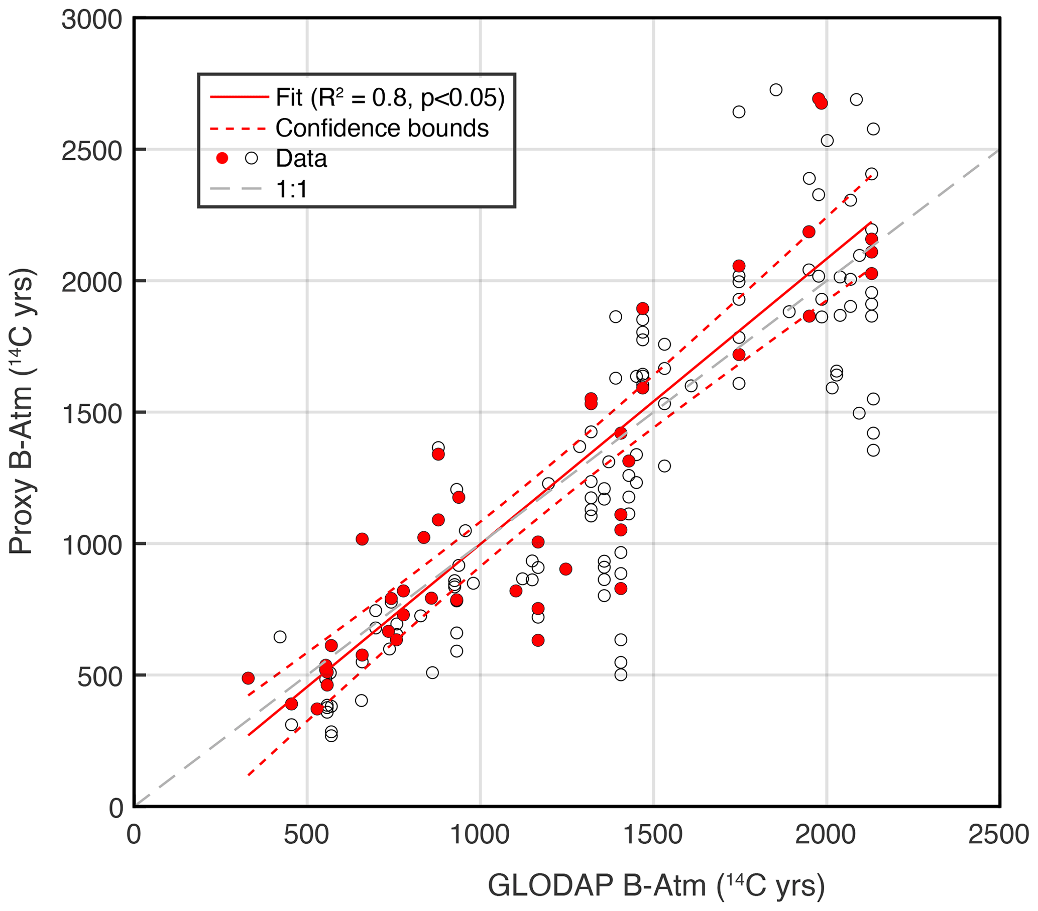
Figure 1Comparison of modern seawater (corrected for the effects of atomic bomb testing) B-Atm radiocarbon age offsets (Key et al., 2004) versus proxy-based B-Atm reconstructions using material deposited during the past ∼ 6000 years (open black circles) and the past ∼ 1500 years (filled red circles). Dashed grey line indicates the 1:1 trend. The linear fit to the data is indicated by the red line (dashed red lines show 95 % confidence limits), with the following equation: , R2= 0.81, p= .
In order to assess the implications of applying the data flags described above, three alternative interpolations were performed: (1) the baseline interpolation, where all flagged data were excluded (Table 1, “Baseline”); (2) as for the baseline but with low sedimentation rate sites (< 2 cm kyr−1) retained (Table 1, “Low sedimentation”); and (3) as for the baseline but retaining only high sedimentation rates > 10 cm kyr−1 (mainly affecting sites in the 2500–4000 m water depth range). In keeping with a similar assessment made by Rafter et al. (2022), we find that the inclusion of very low sedimentation rate sites (< 2 cm kyr−1) has no major effect on our findings, particularly for the global averages (Table 1). The same is true when only retaining sites with very high sedimentation rates > 10 cm kyr−1 (Figs. S2 and S3 in the Supplement), though global averages are biased to slightly lower values (Stott, 2023), particularly at the LGM (Table 1, “High sedimentation”). This apparent lack of sensitivity arises here due to the averaging of a relatively large number of data points (thereby reducing the influence of statistical outliers); however, it should be borne in mind that the inclusion or exclusion of individual data points from sparsely sampled regions (e.g. for the Indian Ocean) can influence the detail of inferred spatial patterns.
Table 1Time-slice global average B-Atm values and their offset from the modern global average B-Atm value, based on 3D interpolations, for three different data flagging approaches, as described in the text: baseline (all flagged data are excluded); low sedimentation (as for baseline but with low sedimentation rate sites included, < 2 cm kyr−1); high sedimentation (as for baseline but retaining only high sedimentation rate sites, > 10 cm kyr−1). Hypothetical corrections for maximum “attenuation biases” and inferred atmospheric CO2 impacts are shown compared with observed mean atmospheric CO2 levels. For each data flag scenario, the total number of deglacial data points and average recorded water depth is shown as a rough indication of the impact of the data flags: as more stringent flags are applied, the data are biased to fewer points at shallower depths.
2.2 Time slices
We isolate data associated with six key time slices based on their calendar ages and associated uncertainties: the LGM (19–21.8 ka BP), Heinrich Stadial 1 (15–17.5 ka BP), the Bølling-Allerød (12.8–14.8 ka BP), the Younger Dryas (YD, 11.8–12.7 ka BP), the early Holocene (EHOL, 9–11 ka BP), and the late Holocene (HOL, < 6 ka BP). Note that the boundaries of these time intervals are informed by, but do not correspond precisely to, their respective ice-core chronozone definitions (Rasmussen et al., 2014). This is due to the generally lower resolution of the marine records and the need to be pragmatic in avoiding, as much as possible, misattributing data to an adjacent chronozone. Where calendar age uncertainties result in an ambiguous assignation of a single time slice, no time slice is assigned.
2.3 Radiocarbon “ventilation” metrics
The term “ventilation” is defined here as comprising the processes that influence physical and chemical property exchanges between the ocean interior and the atmosphere (Skinner and Bard, 2022). Accordingly, the term “(radiocarbon) ventilation age” is not used to refer to “ideal ages” or “transit times” (England, 1995; Marchal and Zhao, 2021b), but rather to the degree of isotopic (14C C) disequilibrium between the ocean and atmosphere, as determined by gas-exchange efficiency and water transport rates (Koeve et al., 2015). In this context “gas-exchange efficiency” is a catch-all term that refers primarily to the gas transfer piston velocity and includes the influence of the mixed layer equilibration time, which in turn depends on, for example, the mixed layer depth.
“Radiocarbon ventilation” must in turn be differentiated from measures of relative isotopic enrichment, such as B-Atm age offsets (Soulet et al., 2016). While `ventilation' refers to a set of processes (principally gas-exchange efficiency and water transport), observation-based metrics such as B-Atm reflect measurements of radiocarbon isotopic disequilibrium, typically between the ocean interior and the atmosphere or mixed layer (Skinner and Bard, 2022). This terminology mirrors a standard geological principle of separating descriptive names (e.g. diamicton) from the inference of process (e.g. glacial till).
In summary, B-Atm should not be used to directly imply transit times or ideal ages, which are not equivalent to “radiocarbon ventilation ages”. Furthermore, metrics such as B-Atm offsets are influenced by a wider variety of processes than just ventilation (i.e. more than just gas exchange and transport), including, for example, atmospheric radiocarbon production changes (Heaton et al., 2021). Therefore, B-Atm offsets should only be used to refer to ventilation (i.e. gas exchange and transport) with caution, as we explore in this study.
2.4 Interpolation
We use the interpolation method described in Skinner et al. (2017), updated to weight input data according to their reported uncertainties. The method interpolates the observed ocean–atmosphere radiocarbon age offset anomalies onto the grid of an ocean model with 24 vertical levels and horizontal resolution. The anomalies are defined relative to the modern GLODAP radiocarbon ages (Key et al., 2004). The interpolating function is constructed using a weighted superposition of radial basis functions centred at the sediment-core locations. These basis functions are built here using an exponential basic function, , with shape parameter, ε. The distance r is defined as the time for tracer impulses to spread out from the core locations to the rest of the grid, based on the modern transport and density stratification. The basis-function weights, the shape parameter, and two hyper-parameters that scale the relative size of the precisions in the prior and likelihood functions are inferred using a three-level Bayesian procedure. (Further details are given in Skinner et al., 2017.) The interpolation process is repeated independently for each time slice so that the data from one time slice do not influence the interpolation for the other time slices.
This interpolation method is somewhat conservative because it is based on the distribution of relative tracer transport and diffusion timescales in the modern ocean. This choice is premised on the need to obtain an interpolated solution in three dimensions that is physically sensible and informed by large-scale oceanographic requirements, including vertical stratification, basin margins/topographic boundaries, and dominant transport pathways (e.g. the Antarctic Circumpolar Current, Deep Western Boundary currents, etc.). It is important to note that the interpolation method does not impose the modern transport on the resulting interpolated fields, nor does it assume strict adherence to the modern density field. Rather, it represents a physically guided and data-constrained anomaly relative to the modern state. The inferred anomalies relax to zero in the absence of data constraints, though some locations in the ocean can have far reaching influence. This method represents a counterpoint to the approach recently taken by Rafter et al. (2022), for example, where spatial interpolations were illustrated for data projected onto 2D sections. In their study, averages were also produced for time series grouped and weighted according to their position within the modern density- and B-Atm distributions (i.e. locations closest to the modern mean for a given basin and density class were weighted to dominate the mean in the past). With this approach, the spatial distribution of density classes is assumed invariant over time, despite the inference of circulation changes. This mirrors to some extent our use of a modern transport field as a guide to the volumetric representativity of individual sample locations. Interpolating a sparsely sampled 3D field is a difficult problem, and a diversity of approaches is surely useful; however, it should be noted that Rafter et al. (2022) did not consider the upper ∼ 1000 m of the ocean and did not produce or discuss global averages.
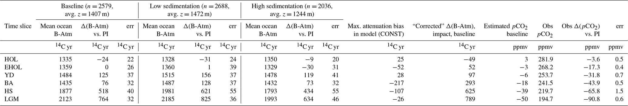
In order to assess the accuracy of the interpolation method of Skinner et al. (2017), and its ability to represent different circulation states, we apply it to a range of modelled radiocarbon fields. For this we use new outputs from the Bern3D model (see below) and pre-existing outputs from the LOVECLIM model (Menviel et al., 2017, 2018). We extract data from the modelled fields at the same locations as the available proxy data (e.g. for the LGM) and attempt to reproduce the modelled global field using the interpolation method. As shown in Fig. 2, the interpolation method is generally successful in reproducing the simulated radiocarbon fields for altered circulation states. The interpolation does best for circulation states characterized by altered wind, diffusivity, and gas exchange, yielding average errors for 1000 randomly selected individual grid cell estimates of RMSE ∼ 276 years (INT_ALL60; this study), RMSE ∼ 244 years (INT_ALL80; this study), RMSE ∼ 398 years (V3LNAw; Menviel et al., 2017), and RMSE ∼ 511 years (V3LNAwSOwSHWw; Menviel et al., 2017) (see Figs. 2 and 3). The interpolation performs slightly less well for extremely different circulation states, e.g. yielding RMSE ∼ 457 years for the HS1 simulation of Menviel et al. (2018) and RMSE ∼ 577 years for the collapsed Atlantic Meridional Overturning Circulation (AMOC) simulation of Menviel et al. (2017), both of which yielded reversed radiocarbon gradients in the Atlantic as compared with today (Fig. 3). Encouragingly, the interpolation method reproduces the modelled fields more accurately than model simulations of the LGM are typically able to match observations (Muglia et al., 2018; Menviel et al., 2017).
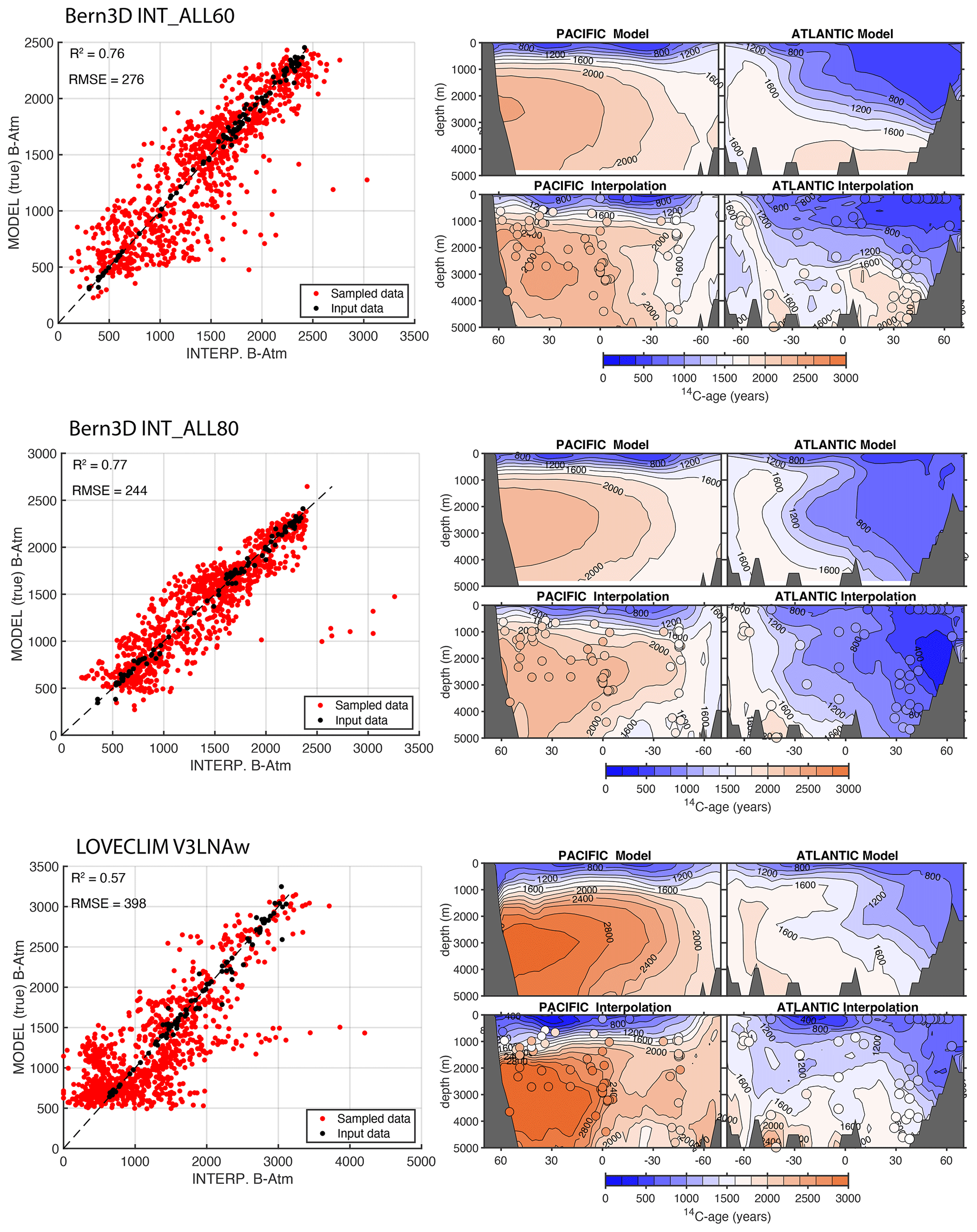
Figure 2Testing the interpolation method using numerical model outputs. Interpolations for the Bern3D and LOVECLIM models, from top to bottom: INT_ALL60 (this study), INT_ALL80 (this study), and V3LNAw (Menviel et al., 2017). Cross plots at left show “true” versus interpolated B-Atm offsets (black circles for input data, red circles for 1000 randomly sampled locations in the ocean interior), with R2 and RMSE shown. Contoured panels show zonally averaged B-Atm offsets (i.e. 14C-age relative to the atmosphere), for the Pacific (left) and Atlantic (right), for both the model output (upper panels) and the interpolated reconstructions (lower panels), with input data used for the interpolations indicated by the filled circles.
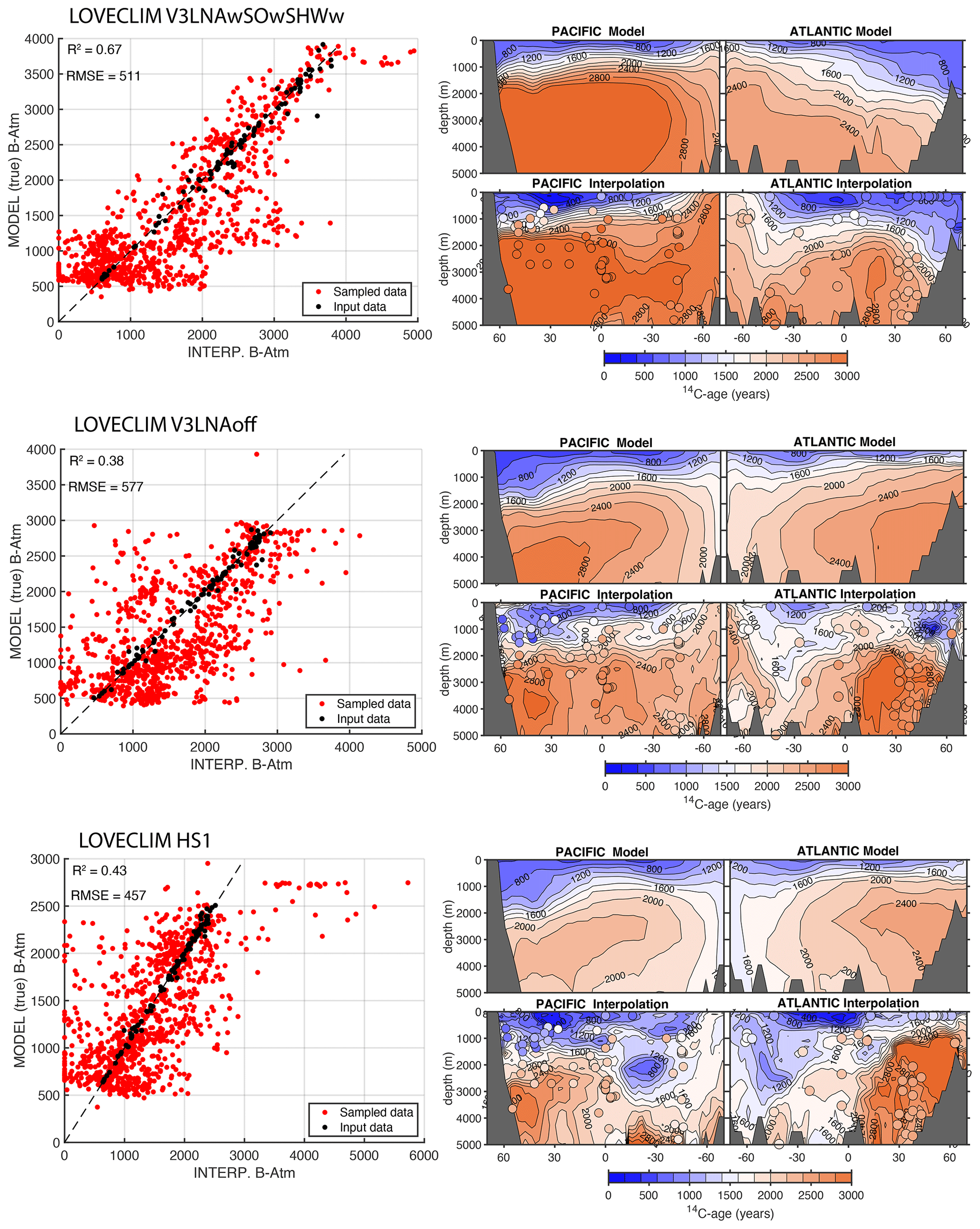
Figure 3Testing the interpolation method using numerical model outputs, as for Fig. 2. Interpolations for simulations using the LOVECLIM model, from top to bottom: V3LNAwSOwSHWw (Menviel et al., 2017), V3LNAoff (Menviel et al., 2017), and HS1 (Menviel et al., 2018). Cross plots at left show “true” versus interpolated B-Atm offsets (black circles for input data, red circles for 1000 randomly sampled locations in the ocean interior), with R2 and RMSE shown. Contoured panels show zonally averaged B-Atm offsets (i.e. 14C-age relative to the atmosphere), for the Pacific (left) and Atlantic (right), for both the model output (upper panels) and the interpolated reconstructions (lower panels), with input data used for the interpolations indicated by the filled circles.
In the present study, the interpolation is primarily intended for calculating global average B-Atm offsets using a relatively sparse dataset (N= 124–476). It is therefore notable that the interpolation reproduces modelled global averages even more accurately than the spatial distributions, with RMSE ∼ 53 years (Fig. 4, circles). In contrast, simple arithmetic means of B-Atm values drawn from a sub-set of locations in the modelled fields consistently underestimate the true global mean by ∼ 274 years on average (Fig. 4, triangles). This comparison underlines the importance of applying a spatially resolved volumetric weighting to the observations for the derivation of accurate global averages. While our interpolation approach leaves room for improvement, it complements alternative data-constrained modelling approaches that have been applied to, for example, the LGM and the YD (Pöppelmeier et al., 2023), and it represents a first step towards addressing the problem of deriving 3D global fields, and appropriately weighted global averages, from sparsely sampled proxy data, without (as yet) the use of forward or inverse models.
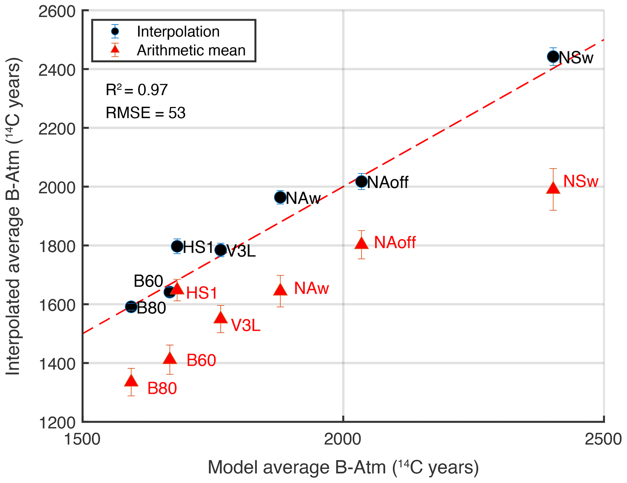
Figure 4Comparison of global average B-Atm offsets based on interpolated fields (circles, with estimated interpolation error), and geometric averages of the input data used for the interpolations (triangles, with standard error), versus the true values for the model simulations shown in Figs. 2 and 3 plus an additional simulation (NAw) from (Menviel et al., 2017). The R2 correlation coefficient, RMSE, and 1:1 line (dashed red line) are indicated.
2.5 Modelling
The intermediate complexity Bern3D v2.0 Earth system model (Ritz et al., 2011; Roth et al., 2014) has been used to explore a series of idealized scenarios that aim to probe the parallel sensitivities of atmospheric CO2 and marine radiocarbon, subject to changes in global vertical diffusivity, Southern Ocean winds, and/or Southern Ocean gas-exchange efficiency. The implementation of radiocarbon in the Bern3D model is described elsewhere (Müller et al., 2006; Müller et al., 2008; Dinauer et al., 2020), and the simulations presented here extend those performed by Jeltsch-Thömmes et al. (2019) and Dinauer et al. (2020), as well as those performed using an earlier version of the Bern3D model by Tschumi et al. (2011). The applied version of the Bern3D model comprises a single-layer energy-moisture balance atmosphere with a thermodynamic sea-ice component (Ritz et al., 2011), coupled to a 3D geostrophic-frictional balance ocean model (Edwards et al., 1998; Müller et al., 2006), and a four-box representation of the land biosphere that simulates the dilution of an atmospheric isotopic perturbation by the land biosphere but here does not address changes in land carbon stocks (Siegenthaler and Oeschger, 1987). Furthermore, marine sediments were not implemented in the model set-up used here, as we sought to isolate the impacts of ventilation processes (i.e. ocean gas exchange and transport).
A first set of sensitivity tests (PI-), performed under “pre-industrial” conditions, and run out for 10 000 years with a fully interactive climate-carbon cycle system (minus sediments), consisted of step changes in (1) global vertical diffusivity in the ocean (Kv), (2) Southern Ocean wind stress (SW), (3) Southern Ocean gas-exchange efficiency or piston velocity (SG), or (4) a combination of Kv, SW, and SG (ALL). In each case the relevant parameter was reduced by 20 %, 40 %, 60 %, or 80 % relative to its baseline value, and impacts were evaluated after 2000 years. (Impacts after 500 and 5000 years are illustrated in Fig. S1.)
In an additional set of simulations, we employed a range of glacial/deglacial scenarios, similar to those of Jeltsch-Thömmes et al. (2019), where each is again defined by idealized adjustments to vertical diffusivity, wind stress, Southern Ocean gas exchange, or a combination of these, as described for the above PI- sensitivity tests. For these simulations, the model was “spun up” into equilibrium over 35 000 model years under pre-industrial (1700 CE) boundary conditions. The model was then ramped linearly over 5000 years from the resulting PI equilibrium state into “glacial” boundary conditions (i.e. representative of 50 ka BP) for ice sheet albedo, greenhouse gas radiative forcing, and insolation, as well as prescribed values for diffusivity, wind stress, and Southern Ocean gas-exchange efficiency as described above. After this, ice-sheet albedo, greenhouse gas radiative forcing, and insolation were varied based on observations since 50 ka BP, with diffusivity, Southern Ocean wind stress, and Southern Ocean gas-exchange efficiency remaining constant for 32 000 years and then relaxing linearly back to PI control values from 18 to 14.6 ka BP, after which PI control values were maintained.
In one set of “glacial/deglacial” model simulations (INT-), atmospheric radiocarbon was prescribed from 50 ka BP based on the Intcal20 reference curve (Reimer et al., 2020). Radiocarbon concentrations in the model were therefore required to be consistent with the observed atmospheric radiocarbon concentration, via changes in the global radiocarbon inventory (which are equivalent to ad hoc changes in radiocarbon production). In a second set of simulations (FIX-) atmospheric radiocarbon activity was held constant at 140 ‰, while in a third set of simulations (CONST-) atmospheric radiocarbon production rates were held constant at the PI value. In each case a control simulation was performed with evolving boundary conditions as described above. A series of additional simulations were then performed with altered global vertical diffusivity (Kv), Southern Ocean wind stress (SW), Southern Ocean gas-exchange efficiency (SG), or a combination of these (see Table S1 in the Supplement). The goal of these transient simulations is not to reproduce the last deglaciation but to assess the sensitivity of both marine radiocarbon and atmospheric CO2 to a variety of changes in ocean ventilation (in terms of both the type of forcing and its magnitude), specifically where concurrent radiocarbon production rate changes are either minimized (CONST-/FIX-) or maximized (INT-).
Figure 5 illustrates zonally averaged radiocarbon age offsets (B-Atm) for the LGM, HS1, BA, and YD, in the Atlantic and Pacific basins, based on global interpolations of the compiled data (using the “baseline” data flags). Differences between each successive time-slice interpolation are shown in Fig. 6. Zonal averages and time-slice offsets for the Indian Ocean are shown in Fig. 7. Zonal averages for the EHOL and HOL, which differ only slightly from the modern field (Key et al., 2004), are shown in Fig. 8 and compared with the interpolated fields for the BA and LGM. As noted elsewhere (Skinner and Bard, 2022; Rafter et al., 2022), the current paucity of data from the Indian Ocean makes interpolations for this basin somewhat tentative and more strongly dependent on individual data points (Fig. 7). This highlights the Indian basin as an important target for future work reconstructing past B-Atm changes. Across all the time-slice interpolations, correlations between observed and interpolated values for the same locations yield R2 values in the range 0.59–0.86. Because the interpolation is not performed on a 2D zonal plane, local B-Atm estimates may deviate from the zonal average where zonal gradients exist. Furthermore, the interpolations necessarily provide an average “snapshot” for an entire time slice and therefore will mask variability within the time slice. These aspects appear to be particularly relevant for HS1 in the Atlantic, as discussed below.
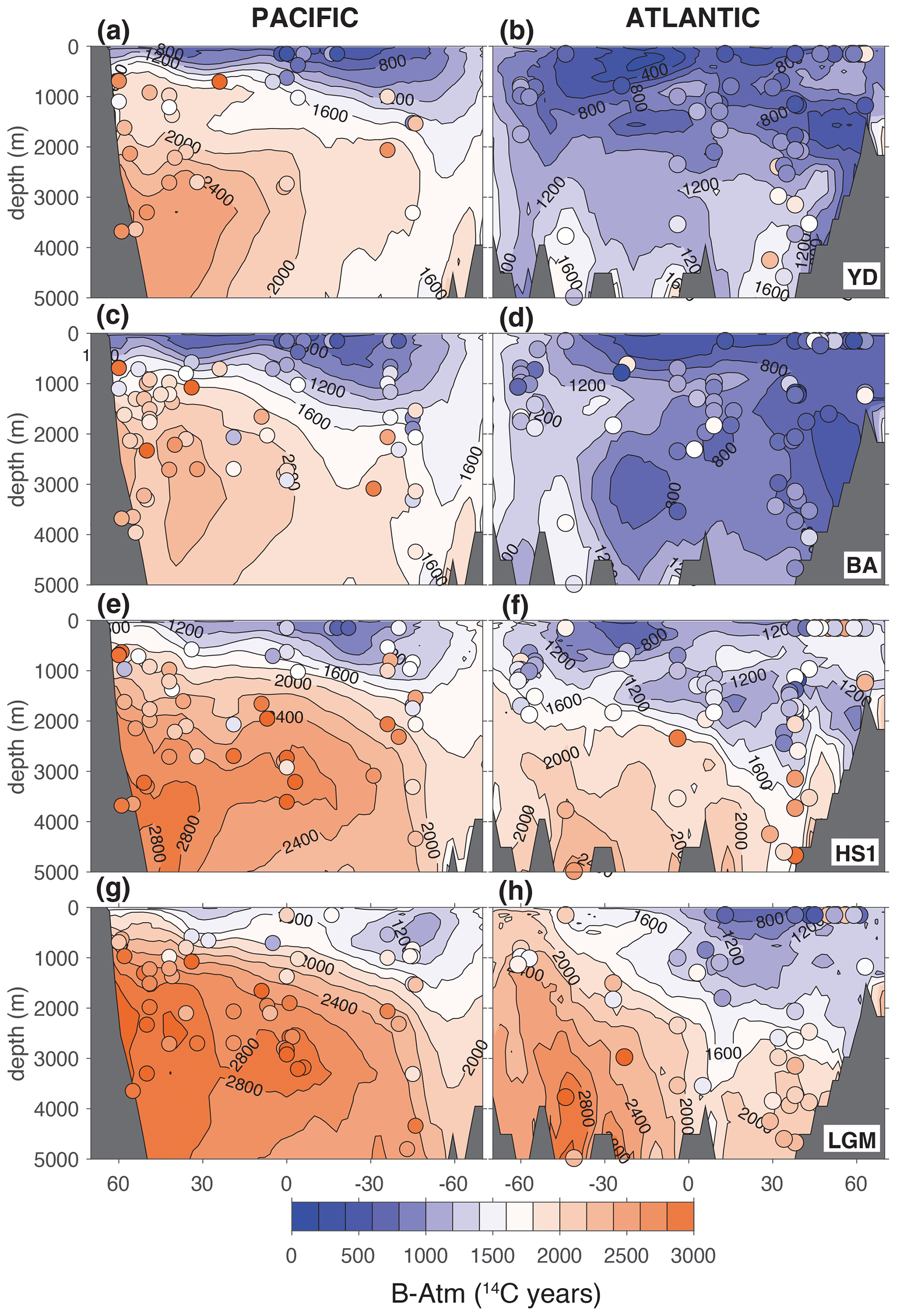
Figure 5Zonally averaged interpolated B-Atm radiocarbon age offsets for the LGM, HS1, BA, and YD (Pacific zonal averages at left, Atlantic at right). Filled circles and shading indicate input data and values.
The global interpolations illustrated in Fig. 5 capture the main features of deglacial B-Atm evolution that have previously been identified in individual time series and in compiled time series that were grouped by basin and region, or water depth (Skinner and Bard, 2022). Broadly similar patterns have also been identified in averaged time series and 2D zonal projection contour plots of compiled data (Rafter et al., 2022). The main features include the following:
-
increased B-Atm offsets throughout the global ocean at the LGM as compared with the modern state (Fig. 8a, b, g, h), in particular > 2000 m water depth as demonstrated previously (Skinner et al., 2017) but with a slightly larger anomaly ∼ 760 14C yr;
-
a stepwise “rejuvenation” of the ocean interior across the last deglaciation;
-
evidence for positive B-Atm anomalies in the deep North Atlantic, from the LGM to HS1 and, again, from the BA to the YD, occurring in parallel with changes of broadly opposite sign in the Southern Ocean and the intermediate depth North Pacific (boxed areas in Fig. 6c, d, g, h);
-
a marked “rebound” to lower B-Atm offsets throughout the ocean, from HS1 to the BA (Fig. 6e, f); and
-
a further rebound to lower B-Atm offsets in the deep North Atlantic, from the YD to the EHOL, again with evidence for changes of opposite sign in the Southern Ocean and intermediate depth North Pacific (boxed areas in Fig. 6a, b).
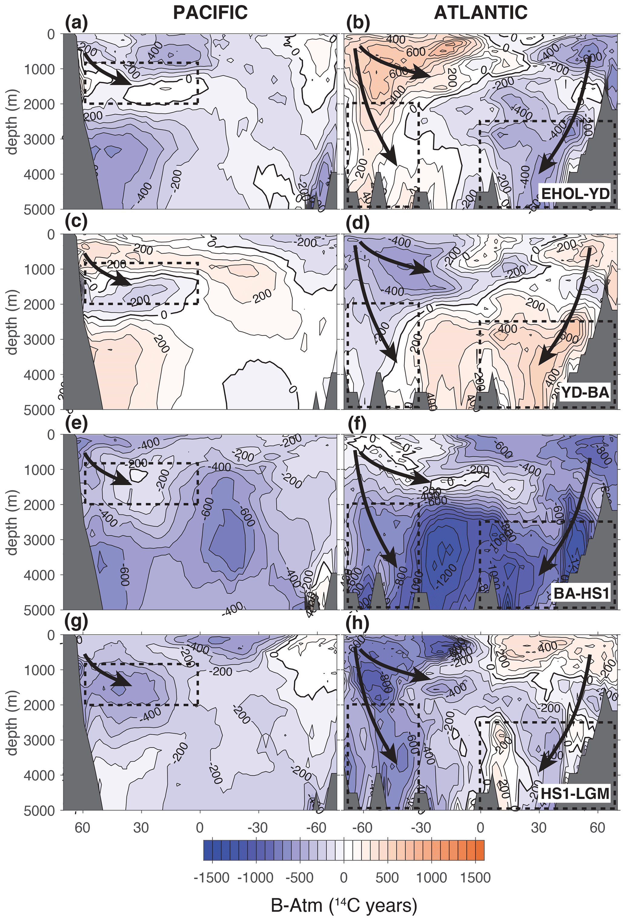
Figure 6Offsets between spatial B-Atm interpolations for successive time-slice reconstructions. Boxed areas highlight regions of the deep North Atlantic (> 0∘ N, > 2.5 km), deep Southern Ocean (> 30∘ S, > 2 km), and intermediate North Pacific (> 0∘ N, 0.9–2 km) and deep North Pacific (> 0∘ N, > 2 km), for which regional time-series splines are illustrated in Fig. 9. Broadly antiphased anomalies are indicated between the North Atlantic and Southern Ocean (especially the Atlantic sector), and between the North Atlantic and intermediate North Pacific.
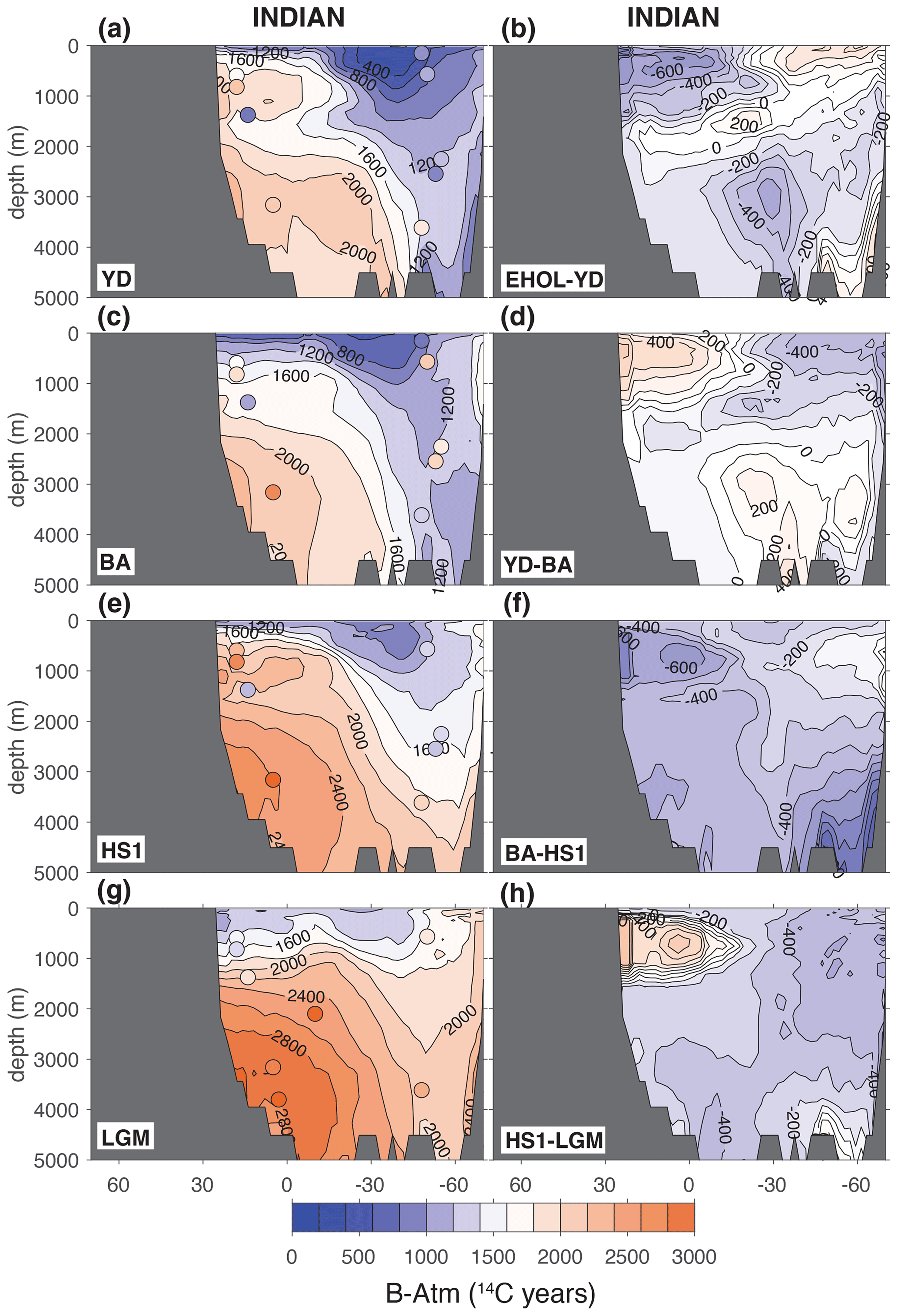
Figure 7Zonally averaged interpolated B-Atm radiocarbon age offsets in the Indian Ocean for the LGM, HS1, BA, and YD. Sparse data coverage is notable. Left: interpolated time-slice reconstructions (as for Fig. 5). Right: offsets between spatial B-Atm interpolations for successive time-slice reconstructions (as for Fig. 6).
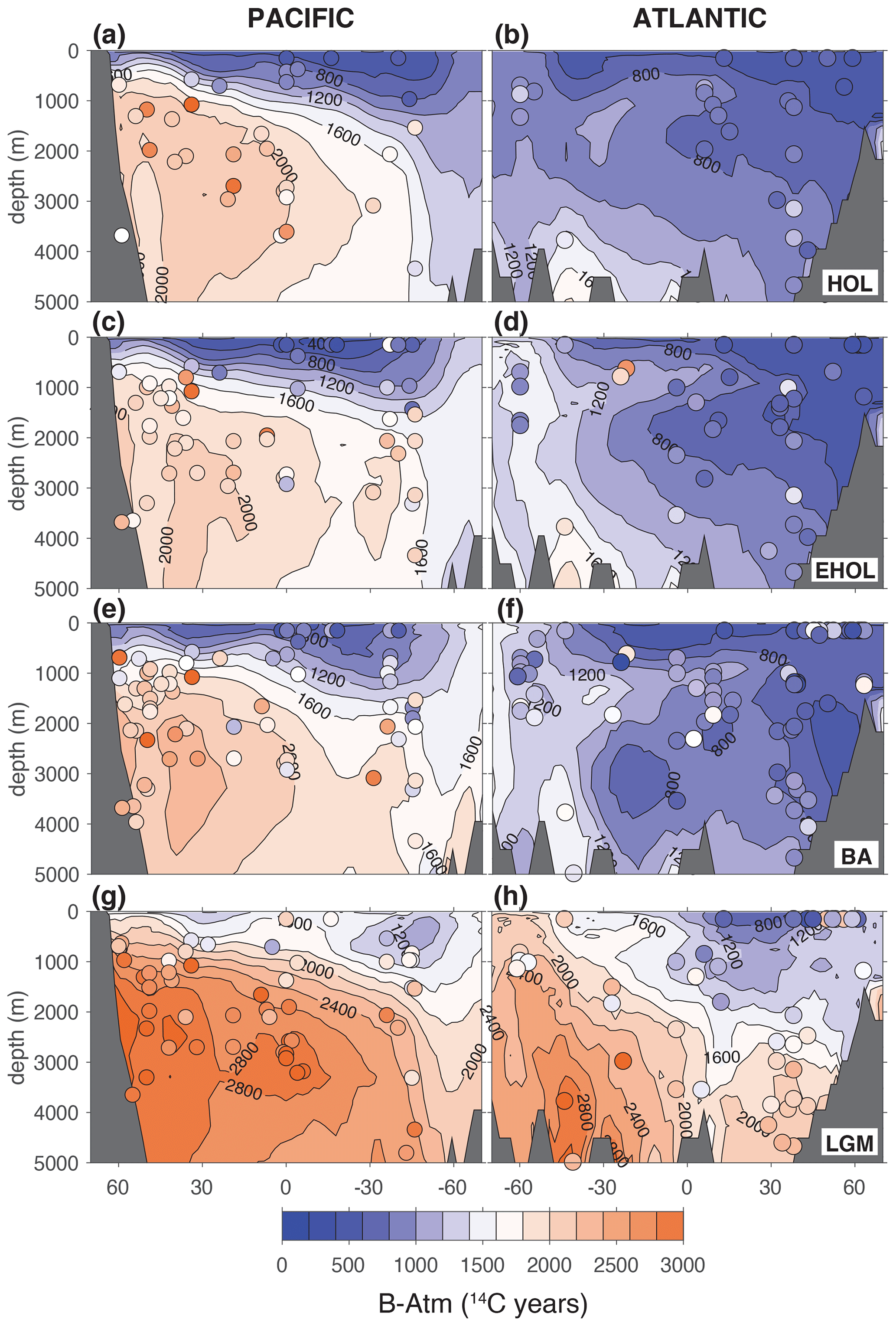
Figure 8Zonally averaged interpolated B-Atm offsets for the LGM, BA, EHOL, and HOL (Pacific zonal averages at left, Atlantic at right). Filled circles and shading indicate input data and values.
Perhaps the most striking aspect of the successive time-slice reconstructions is the marked drop in B-Atm offsets that coincides with the transition from HS1 to the BA (Fig. 6e, f), which involved positively correlated changes in B-Atm in the deep Southern Ocean and deep North Atlantic (Skinner et al., 2013), and which has been linked to an “overshoot” in B-Atm offsets at some locations (Barker et al., 2010; Hines et al., 2015). Notably, as shown in Fig. 8, the step change at the BA resulted in a global B-Atm distribution very similar to that of the late Holocene, despite representing the approximate temporal midpoint of deglaciation.
The features identified above can also be discerned in regional time-series averages (Skinner and Bard, 2022; Rafter et al., 2022). We show this here using cubic splines for North Atlantic, Southern Ocean, and North Pacific data grouped according to the boxed areas highlighted in Fig. 6. The resulting regional average splines are illustrated in Fig. 9b–d compared with global average B-Atm values derived for each successive time slice (Fig. 9d, filled circles; Table 1). During HS1 and the YD, the regional splines exhibit broadly antiphased trends in B-Atm between the deep North Atlantic and the deep Southern Ocean and intermediate North Pacific (Fig. 9, shaded vertical bars). The collected time series thus support the antiphase patterns apparent in the zonal averages shown in Fig. 6 (boxed areas). The averaged time series only tentatively support the suggestion of a “flipped” vertical radiocarbon gradient between the intermediate- and deep North Pacific at the LGM (Rafter et al., 2022), and more emphatically demonstrate this for the deglacial period that includes the YD, BA, and HS1. Indeed, during the BA, the North Pacific, North Atlantic, and Southern Ocean all exhibit B-Atm offsets at least as low as modern, resulting in global average B-Atm that also approaches the modern value and slightly “overshoots” relative to the subsequent YD (see Fig. 9d). Consistent with the fact that the Pacific accounts for ∼ 50 % of the global ocean volume and the Southern Ocean ventilates ∼ 58 % of the ocean interior (Primeau, 2005), Fig. 9 also shows that global average B-Atm estimates generally track the deep North Pacific and the deep Southern Ocean. Different patterns of variability are expressed in the North Atlantic and the intermediate North Pacific, where more rapid and regionally important fluctuations are apparent (Freeman et al., 2015).
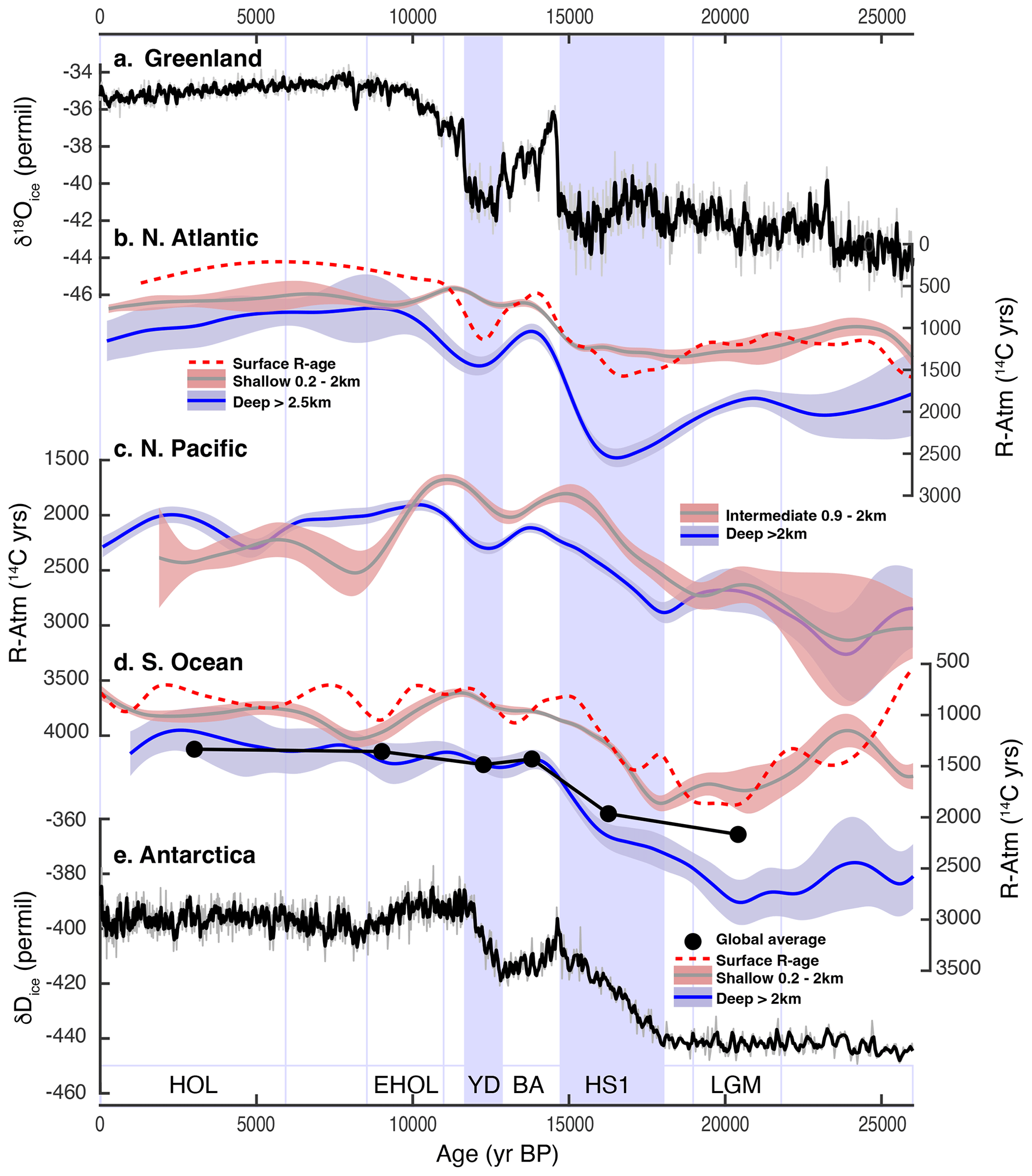
Figure 9“Ventilation seesaws” across the last deglaciation based on cubic spline fits to compiled ocean–atmosphere radiocarbon age offsets (Skinner and Bard, 2022). Cubic splines with a stiffness factor of 10−9 are fit to all existing data, using updated age models and taking into account B-Atm uncertainties, and applying the same “baseline” data flags as for the time-slice interpolations. (a) Greenland temperature proxy (Svensson et al., 2008). (b) northeast Atlantic shallow sub-surface reservoir ages (dashed red line; Skinner et al., 2019); B-Atm from the North Atlantic 0.2–2 km (grey line, shaded red area); B-Atm from the deep North Atlantic > 2.5 km (blue line, shaded blue area). (c) B-Atm from the intermediate North Pacific 0.9–2 km (grey line, shaded red area); B-Atm from the deep North Pacific > 2km (blue line, shaded blue area). (d) Mean ocean B-Atm estimates (black line and circles; see Table 1 “baseline” data flags) and compiled shallow sub-surface reservoir ages from the Southern Ocean (dashed red line; Skinner et al., 2019); B-Atm from the Southern Ocean < 2 km (grey line and shaded red area); B-Atm from the deep Southern Ocean > 2 km (blue line and shaded blue area). (e) Antarctic temperature proxy (EPICA Community Members, 2004; Lemieux-Dudon et al., 2010). Vertical lines and shaded bars indicate the timing of the LGM, HS1, BA, YD EHOL, and HOL time slices.
In principle, evolving large-scale patterns of ocean–atmosphere radiocarbon age offsets (B-Atm) will primarily reflect the combined influences of (1) radiocarbon production, (2) ocean transports, (3) air–sea gas-exchange efficiency (especially in the regions of deep-water export), and (4) the changing contributions of different source regions to locations in the ocean interior. While the influence of atmospheric radiocarbon production changes on evolving B-Atm offsets is often ignored, it may in principle influence deep ocean B-Atm offsets through relatively rapid (i.e. sub-millennial) changes in atmospheric radiocarbon activity that are only conveyed to the deep ocean on the millennial timescale of ocean turnover (Adkins and Boyle, 1997). This can produce a convergence or divergence of marine and atmospheric radiocarbon ages, due to atmospheric radiocarbon changing quickly and the deep ocean remaining relatively invariant (Franke et al., 2008; Heaton et al., 2021).
Below, we discuss how all these processes have influenced marine radiocarbon cycling across the last deglaciation. Accordingly, we address (1) evidence for the operation of a “ventilation seesaw” that we emphasize was linked to both gas-exchange and transport anomalies emanating from the main regions of deep- and intermediate water formation (i.e. the North Atlantic, Southern Ocean, and North Pacific); and (2) the potential for atmospheric radiocarbon dynamics (independent of ocean ventilation) to bias B-Atm offsets by ∼ hundreds of 14C yr, in particular during the apparent BA “overshoot”. We further seek to quantify the likely carbon cycle impacts associated with the observed global average B-Atm changes, and to reconcile these impacts with the evolution of the global radiocarbon budget since the last glacial period.
4.1 Ventilation “seesaws”: gas-exchange and transport effects
A survey of the modern ocean's transport pathways indicates that ∼ 86 % of the ocean interior is sourced by water that last made contact with the atmosphere in three key regions: the Southern Ocean (contributing ∼ 58 %), the high latitude North Atlantic (contributing ∼ 21 %), and the North Pacific (contributing ∼ 7 %) (Primeau, 2005). These three regions account for ∼ 31 % of the ocean's surface and “ventilate” ∼ 86 % of the ocean's interior (Primeau, 2005). Although the long equilibration time for dissolved Δ14C(DIC) means that a water parcel's point of last contact with the atmosphere will not necessarily be equivalent to its point of “radiocarbon equilibration” (high latitude sources are typically characterized by distinct levels of disequilibrium (Bard, 1988; Matsumoto, 2007), changes in the three main regions of deep-water export will exert a strong influence on temporal variations in the ocean interior's radiocarbon distribution.
This expectation is clearly borne out in the global interpolations shown in Figs. 5 and 6, and in the regional stacks illustrated in Fig. 9. Deglacial changes in marine radiocarbon distribution were apparently dominated by anomalies extending from the North Atlantic (affecting the deep Atlantic in particular), coordinated with anomalies of broadly opposite sign originating in the Southern Ocean and North Pacific (Figs. 6 and 9). The time-slice interpolations and regional averages therefore cohere with numerous previous proposals for “ventilation seesaws” operating between the North Atlantic and the Southern Ocean (Broecker, 1998; Skinner et al., 2013, 2014; Menviel et al., 2018), and between the North Atlantic and North Pacific (Menviel et al., 2014; Freeman et al., 2015; Max et al., 2014; Okazaki et al., 2010; Walczak et al., 2020).
As suggested previously (Skinner et al., 2019; Skinner and Bard, 2022), Fig. 9 also shows that B-Atm offsets in the deep (> 2 km) North Atlantic (Fig. 9b, blue line and shaded area) exhibit a similar pattern of variability to that of the upper ocean (0.2–2 km) and surface “reservoir ages” in the region (Fig. 9b grey lines with shaded area, and dashed red lines). The same is apparent in the Southern Ocean (Fig. 9d). These relationships, and their further link to polar climate variability (Fig. 9a, e), suggest a mechanistic link between the observed deglacial B-Atm variability and the “thermal bipolar seesaw” (Stocker and Johnsen, 2003; EPICA Community Members, 2006). This association most likely operated via coordinated changes in North Atlantic and Southern Ocean convection and advection (Broecker, 1998; Menviel et al., 2015; Skinner et al., 2014, 2020) associated with regional changes in sea ice (Skinner et al., 2019; Rae et al., 2018), winds (Sikes et al., 2016b; Menviel et al., 2018), and/or buoyancy forcing (Ferrari et al., 2014; Hines et al., 2019; Watson et al., 2015). The further coupling between the Southern Ocean and North Pacific has been proposed to relate to freshwater balance in the Pacific basin (Menviel et al., 2014), possibly influenced by changing moisture transports across the Isthmus of Panama (Leduc et al., 2007), and/or Cordilleran ice mass balance (Walczak et al., 2020).
While the “ventilation seesaws” noted above may reflect changes in ocean circulation to some extent, it is important to note that they also reflect changes in gas-exchange efficiency. This is demonstrated by the fact that
the amplitude of B-Atm variability in the shallow Atlantic 0.2–2 km water depth (e.g. Freeman et al., 2015; Chen et al., 2015) differs very little from that of surface “reservoir ages” in the northeast Atlantic (Fig. 9b, grey line and dashed red line). This implies a muted contribution from flow speed changes in the upper Atlantic < 2 km (Bradtmiller et al., 2014) and a dominant influence on radiocarbon signatures from gas-exchange (i.e. “pre-formed ages”) instead. Again, the same is true for the Southern Ocean, where B-Atm offsets from the shallow ocean (0.2–2 km) generally overlap with surface reservoir age reconstructions (Fig. 9d, grey line and dashed red line). Accordingly, B-Atm values at the LGM in mid-depths may indeed have been consistent with the modern transport (Marchal and Zhao, 2021a).
In contrast, however, “pre-formed ages” cannot account for the amplitude of B-Atm changes observed in the deep Atlantic (Fig. 9b, blue line) and the deep Southern Ocean (Fig. 9d, blue line), indicating a more significant contribution from water sourcing and/or transport changes > 2 km, and perhaps between 2 and 3 km water depth in particular (Skinner et al., 2021; Lund et al., 2015; Rafter et al., 2022). The patchy response seen in the zonal average anomaly for the North Atlantic between HS1 and the LGM (Fig. 6h) contrasts with the clearer signal seen in individual and collected time series (Fig. 9b). In part, this likely reflects a spatially heterogeneous hydrographic response, both in the depth domain (Skinner et al., 2021; Lund et al., 2015) and in the eastern versus western North Atlantic (Gherardi et al., 2005; Ng et al., 2018). This interpretation is supported by the less ambiguous positive B-Atm anomaly seen in the deep North Atlantic regional time-series spline during HS1 (Fig. 9b, blue line and shaded area; see also Rafter et al., 2022).
The patchy spatial interpolation outcome for HS1 may also reflect a more complex pattern of ventilation during HS1 than is captured by a “collapsed AMOC” scenario that lasted until the onset of the BA, as indicated by a recent multi-proxy and modelling study (Pöppelmeier et al., 2023). Furthermore, in addition to tentative evidence for a “mid-HS1 B-Atm minimum” (Skinner and Bard, 2022), there is evidence for a drop in B-Atm offsets at intermediate depths (< 2.5 km) in the western Atlantic late in HS1 (Robinson et al., 2005; Thiagarajan et al., 2014), and evidence for declining B-Atm offsets in the Nordic Seas ∼ 400 years prior to the onset of the BA (Muschitiello et al., 2019). Any such changes during HS1 will have been averaged out in our time-slice interpolation for 15–17.8 ka BP. These observations underline the need for further detailed reconstruction of the spatial expression and temporal evolution of ocean–atmosphere radiocarbon offsets across the North Atlantic during HS1, particularly with a view to disentangling transport and gas-exchange impacts.
Overall, the message that emerges from the collected data is that deglacial marine B-Atm changes throughout the global ocean were significantly influenced by both air–sea gas-exchange effects and mass transport effects (Koeve et al., 2015), with the latter primarily affecting parts of the deep ocean > 2 km, but with evidence for a complex response during HS1. The inferred spatial expression and coordination of both gas-exchange and transport effects in the Atlantic may have been related to changes in the spatial extent of different water masses in the deep ocean. This would be consistent with previous work where B-Atm offsets have been found to place stronger constraints on water mass “geometry” than, for example, AMOC strength per se (Muglia and Schmittner, 2021; Pöppelmeier et al., 2023). The influence of further non-ventilation effects at each time-slice is taken up in the following section.
4.2 “Attenuation biases” in B-Atm offsets at the BA
As noted above, global average B-Atm changes can occur independently of ventilation effects, due to rapid atmospheric radiocarbon variability to which the deep ocean is too slow to respond. We refer to such effects as “attenuation biases”, as they reflect the phase and attenuation response of a slowly adjusting reservoir (the global ocean interior), subject to continuous exchange with a more rapidly changing reservoir (the atmosphere) (Maier-Reimer and Hasselmann, 1987). The primary external (i.e. non-marine) driver for rapid atmospheric radiocarbon variability is likely to be changes in radiocarbon production (Köhler et al., 2022), though transient terrestrial carbon sources (e.g. from permafrost) might also be hypothesized (Köhler et al., 2014; Wu et al., 2022).
For attenuation biases in mean ocean B-Atm offsets to occur, atmospheric radiocarbon activity would have to change rapidly, that is, on a timescale that is shorter than the mean mixing time of the ocean (i.e. < 1000 years). Accordingly, gradual long-term trends in radiocarbon production are unlikely to produce significant attenuation biases, as is confirmed by model simulations where atmospheric radiocarbon production is based on relatively smooth trends in mean relative (geomagnetic) palaeointensity (RPI) (Dinauer et al., 2020). However, given the scatter amongst existing reconstructions of past radiocarbon production (e.g. Laj et al., 2004; Adolphi et al., 2018; Nowaczyk et al., 2013; Channell et al., 2018), particularly on (sub-) millennial timescales, it remains unclear to what extent rapid (centennial or millennial) radiocarbon production variability and/or other non-marine carbon sources might have biased B-Atm offsets via their impact on the atmosphere. Therefore, to explore the maximum possible contribution of externally driven atmospheric radiocarbon variability to mean ocean B-Atm changes, we compare transient simulations using the Bern3D model where radiocarbon production rates or atmospheric radiocarbon are held constant (i.e. FIX- and CONST-, respectively) with simulations where nearly all variability in atmospheric radiocarbon is assumed to have occurred independently of ocean ventilation change (i.e. INT-, where atmospheric radiocarbon is prescribed according to Intcal20). The difference between the INT- simulations and their CONST/FIX- counterparts yields the maximum amplitude of B-Atm changes that could be produced independently of ocean ventilation change, for each idealized scenario. Indeed, as discussed below, these estimates are likely over-estimates as they are premised on the assumption that all atmospheric radiocarbon variability occurred independently of ocean–atmosphere radiocarbon exchange, which is unlikely.
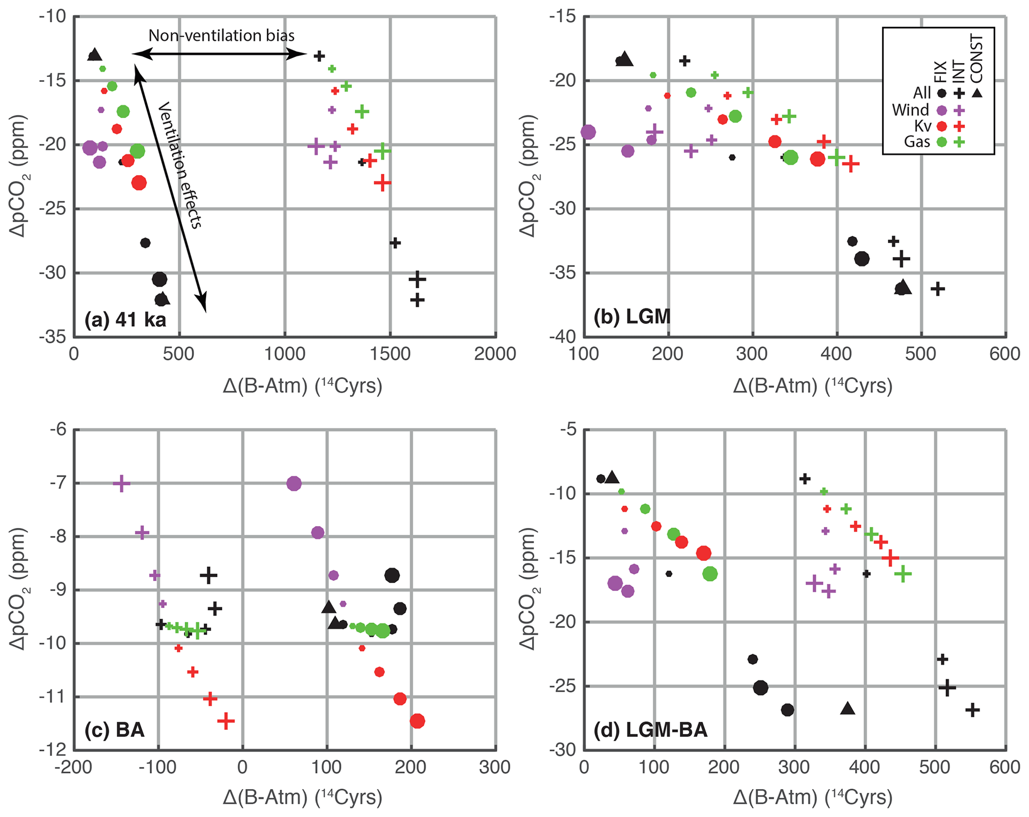
Figure 10Model outputs from idealized “deglacial” scenarios illustrating hypothetical attenuation biases that are unrelated to ocean “ventilation” effects (indicated by horizontal offsets between similar symbol colours; horizontal arrow in panel (a). Panel (a)shows 41 ka BP (coinciding with the Laschamps geomagnetic excursion), (b) the LGM, (c) the BA, and (d) the offset between the LGM and the BA. Data are expressed as 1000-years average anomalies relative to the pre-industrial period 4–5 ka BP, when atmospheric radiocarbon was relatively stable and therefore plausibly approached a pseudo-equilibrium state. In all panels, crosses indicate model experiments carried out with prescribed atmospheric radiocarbon as given by Intcal20 (Reimer et al., 2020) (INT), circles are for atmospheric radiocarbon fixed at 140 ‰ (FIX), and triangles are for constant pre-industrial radiocarbon production rates (CONST). Symbol colours distinguish experiments carried out with altered Southern Ocean winds (purple), vertical diffusivity (red), Southern Ocean gas-exchange efficiency (green), or all combined (black). Four symbol sizes indicate the extent of parameter reduction: 0 % (control, smallest symbols), 20 %, 40 %, 60 %, and 80 % (largest symbols). For CONST, only two sets of experiments were run: for control conditions and for all tuning variables reduced by 60 %. Note that the impact on B-Atm due to reduced Southern Ocean winds (purple circles) is attenuated in well-equilibrated states (e.g. 41 ka and LGM), because of, for example, slow adjustments in the distribution of North Atlantic sourced deep water (see text).
As illustrated in Fig. 10 (and summarized in Table S1), our idealized scenarios demonstrate three key points regarding the emergence of “attenuation biases” in B-Atm offsets:
-
These biases depend on the occurrence of rapid atmospheric variability that is not forced by ocean ventilation change, but they can in principle result in persistent long-term biases via an accumulation of centennial or millennial perturbations (e.g. as for a “random walk” process).
-
Such biases are time varying and may be positive relative to a given reference time (e.g. at the Laschamps event; Fig. 10a), negative (e.g. notably, at the BA onset; Fig. 10c), or nil (e.g. at the LGM; Fig. 10b), thus enhancing, diminishing, or not affecting the B-Atm changes that are expressed between time periods (Fig. 10d).
-
The relative contribution of such biases will be diminished and potentially eliminated to the extent that they coincide with large abrupt ocean ventilation changes (not included in our idealized model simulations), though it is apparent that their magnitude depends mainly on the amplitude of atmospheric radiocarbon production changes, as they yield a relatively invariant offset between the INT- and CONST/FIX- simulations for any given time slice; Fig. 10a–d).
It is important to stress that the true magnitude of such attenuation biases cannot be determined without prior detailed knowledge of the history and magnitude of both ocean ventilation changes and non-marine carbon and/or radiocarbon inputs to the atmosphere. Nevertheless, two observations are worth underlining: the first is that maximum estimates of the attenuation biases that could hypothetically affect deglacial B-Atm offsets would only result in relatively minor biases in the incremental B-Atm changes between time slices (ranging from −227 to +25 14C yr). Even if maximal attenuation biases are hypothesized, the observed deglacial mean ocean B-Atm trends must include a significant ventilation contribution. Indeed, such changes are directly attested to by proxy evidence for ocean transport and sea-ice change (McManus et al., 2004; Schüpbach et al., 2018), as well as the spatially heterogeneous patterns in marine B-Atm offsets that we present here (e.g. Figs. 6 and 9).
A second key observation is that correcting for such biases would tend to diminish the apparent “ventilation surge” that might be inferred from the change in B-Atm between HS and the BA (and more so between the LGM and the BA). Thus, if the rapid atmospheric radiocarbon decline across HS1 and at the onset of the BA were entirely driven by radiocarbon production changes and/or non-marine carbon inputs to the atmosphere, then the change in global average B-Atm between the LGM and the BA would be biased by at most ∼ 227 14C yr. In this case, radiocarbon ventilation ages during the BA would be ∼ 227 14C yr older than inferred from observed B-Atm offsets, resulting in a smaller radiocarbon ventilation change between the LGM and the BA. Non-ventilation biases affecting global average B-Atm differences between the LGM and the BA could therefore imply a smaller contribution from gas-exchange and transport rate changes to the apparent radiocarbon “ventilation surge” suggested for the BA in Fig. 6e and f. In this case, the “rejuvenation” of the marine radiocarbon pool may not in fact have been completed midway through deglaciation as initially apparent (Rafter et al., 2022). This inference would be more consistent with stable carbon isotope (13C 12C) evidence (Sikes et al., 2016b), which suggests an ongoing contribution to ocean–atmosphere carbon exchange well beyond the BA. Indeed, a significant portion of the convergence between marine and atmospheric radiocarbon observed at the BA may have been driven by “old” carbon release to the atmosphere, e.g. from melting permafrost (Köhler et al., 2014; Wu et al., 2022).
Although they remain difficult to accurately quantify, “attenuation biases” unrelated to ventilation are important to acknowledge, as these may exert a subtle yet potentially significant influence on our interpretation of transient changes in B-Atm offsets and their quantification, as illustrated above for the BA. These effects will need to be explored in greater detail in the future, a task that will inevitably require the use of numerical models and also require accurate knowledge of past radiocarbon production changes (Köhler et al., 2022; Dinauer et al., 2020). The accuracy of our existing radiocarbon production records is discussed further in Sect. 4.4.
4.3 Ventilation-related atmospheric CO2 change
In theory, a broadly linear relationship between atmospheric CO2 change and global average marine radiocarbon age anomalies is to be expected when these are driven by gas-exchange and/or transport rates (Skinner and Bard, 2022; Skinner et al., 2017). This is because (1) longer residence times in the ocean interior result in greater respired carbon accumulation along with greater radiocarbon decay, and (2) restricted gas exchange in regions of “upwelling” and/or deep mixing impede the conversion of respired and/or disequilibrium carbon to equilibrium carbon (Eggleston and Galbraith, 2018) while also impeding the invasion of radiocarbon into the ocean.
Our model sensitivity tests, involving shifts in vertical diffusivity, Southern Ocean winds, and/or gas exchange, cohere with a number of existing simulations using box models and Earth system models of intermediate complexity (e.g. Tschumi et al., 2011; Kwon et al., 2011; Skinner and Bard, 2022), confirming a broad relationship between B-Atm anomalies and associated atmospheric CO2 change (Fig. 11a, Table 2), despite large differences in model experiment set-up. These experiments include the effects of pCO2 changes on air–sea 14C exchange (Galbraith et al., 2015; Bard, 1988). Our sensitivity tests indicate consistent sensitivities for individual suites of experiments, e.g. for varying Southern Ocean winds, vertical diffusivity, or Southern Ocean gas-exchange rates. However, depending on the processes responsible for altering deep ocean ventilation, modelled sensitivities span a range of approximately ±50 % for a given magnitude of B-Atm change. Furthermore, the sensitivities may vary with perturbation timescale, with different impacts on millennial timescales than on glacial-interglacial or longer timescales (Jeltsch-Thömmes and Joos, 2020). For example, a reduction in Southern Ocean winds draws down atmospheric CO2 and increases global average B-Atm on a timescale of ∼ 2000 years via impacts on gas-exchange rates and upper ocean turnover (Fig. 11a). However, after ∼ 5000 years (see Fig. S1) the mean ocean B-Atm response is diminished, primarily due to the spin up of North Atlantic deep water, which replaces southern sourced water in the deep Atlantic. A muted B-Atm response can therefore be seen for stronger Southern Ocean wind forcing in the 50 ka simulations illustrated in Fig. 10a (purple symbols). Despite their potential role in transient millennial scale pulses, Southern Ocean winds are therefore unlikely to account for long-term glacial-interglacial B-Atm changes, at least in the absence of further forcing to suppress North Atlantic ventilation (Menviel et al., 2018).
Table 2B-Atm and atmospheric CO2 results for sensitivity experiments carried out using the Bern3D model with varying Southern Ocean (SO) wind, gas exchange, or global vertical diffusivity (illustrated in Fig. 10). Results are evaluated 2000 years after forcing is applied (see text).
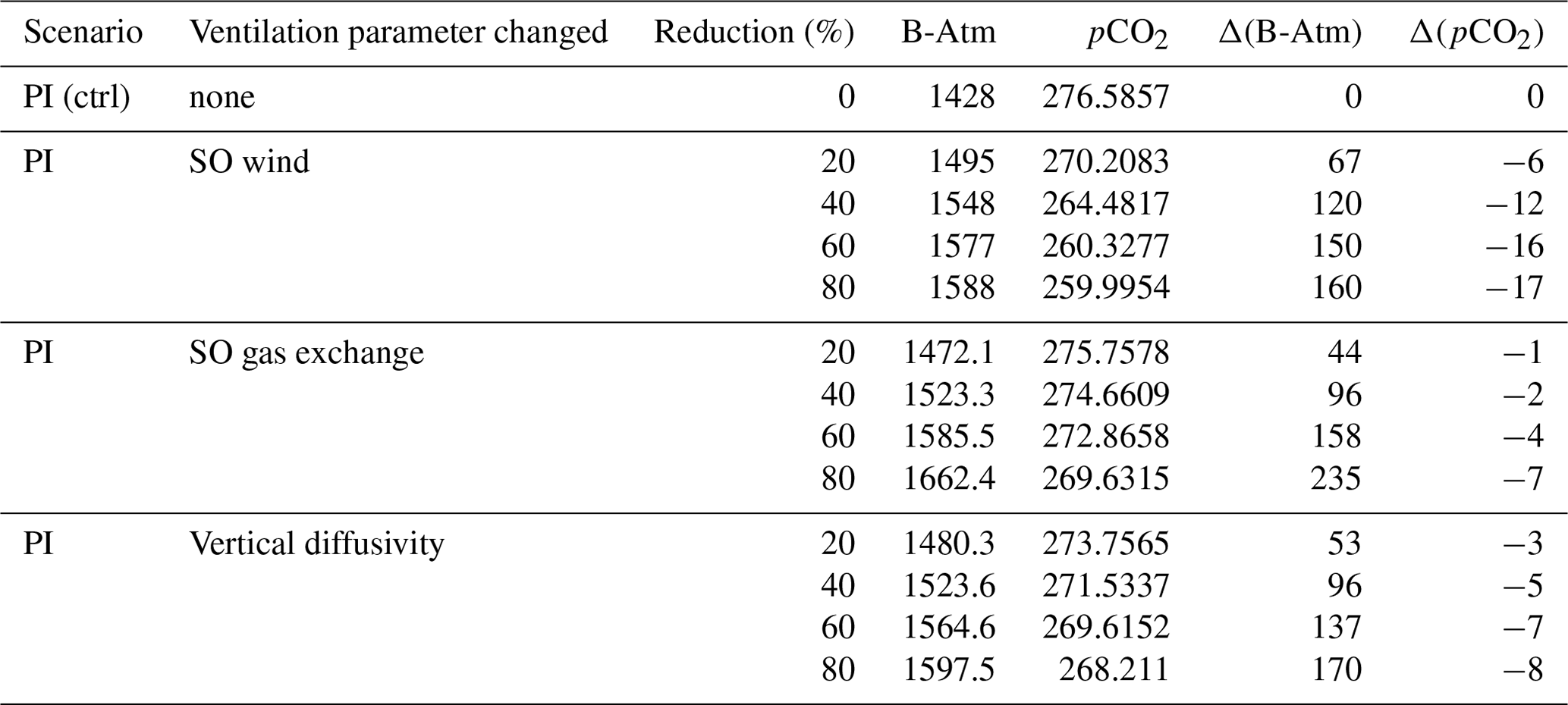
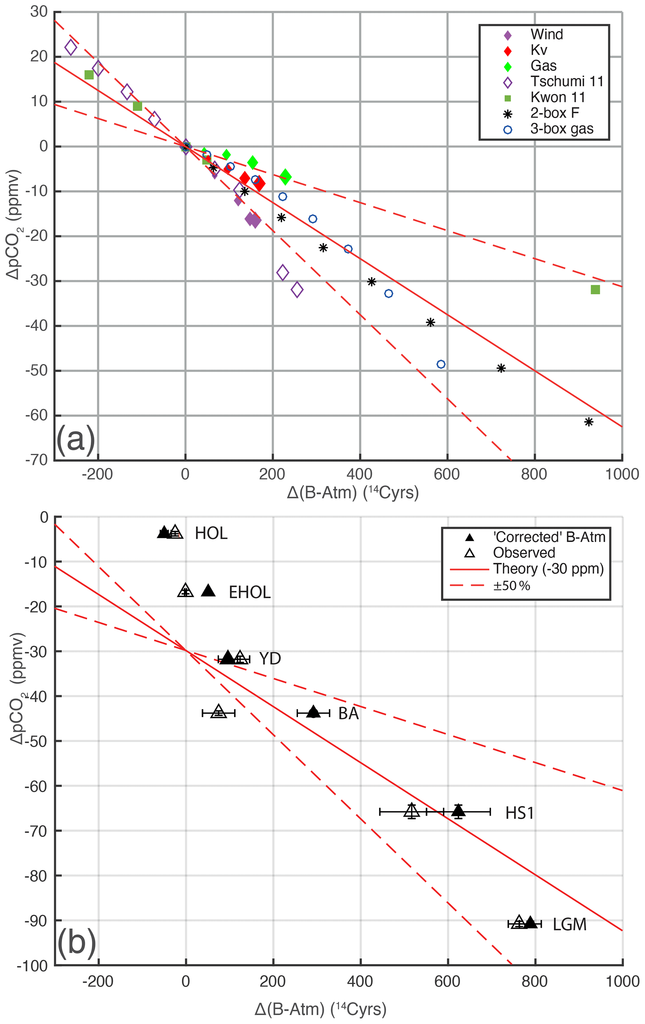
Figure 11Panel (a)shows theoretical and modelled sensitivity of atmospheric CO2 anomalies and mean ocean radiocarbon ventilation age (B-Atm) anomalies to air–sea gas-exchange and transport changes. Filled diamonds indicate model sensitivity tests from this study, based on step changes under PI conditions and 2000 years of equilibration time (purple: Southern Ocean wind, red: vertical diffusivity, green: Southern Ocean gas-exchange efficiency). Open diamonds are Southern Ocean wind experiments (Tschumi et al., 2011). Filled squares are wind and/or diffusivity experiments using an idealized radiocarbon-like tracer (Kwon et al., 2011). Asterisks and open circles represent two- and three-box model experiments, with varying overturning rates (F) and “high latitude” gas-exchange rates (gas), respectively. A median theoretical sensitivity is indicated by the solid and dashed red lines, derived for the two-box model results (Skinner and Bard, 2022), equivalent to ppm CO2 change per 100 14C yr of global radiocarbon ventilation age change. Panel (b)shows observed values of coincident global average B-Atm and atmospheric pCO2, expressed as time-slice anomalies versus pre-industrial values. Open triangles show paired observations of mean ocean B-Atm (this study) and atmospheric CO2 (Monnin et al., 2001; Marcott et al., 2014). Filled triangles show observed B-Atm age offsets corrected for hypothetical “non-ventilation” biases (see text). Solid and dashed red lines in (b) show the same theoretical sensitivities as for (a), offset by −30 ppm to aid comparison with observed trends.
The broadly linear scaling apparent in the suite of PI model sensitivity tests is consistent with basic theory (Skinner et al., 2017; Skinner and Bard, 2022), based on a two-box ocean connected to an atmosphere to form a closed system (Fig. 11a, solid line). This simple inventory theory predicts a higher sensitivity for higher global export productivity and/or a higher “Revelle buffer factor” (i.e. higher background atmospheric pCO2), all else being equal. Clearly, the marine carbon cycle response to the variety of ventilation processes that can affect radiocarbon cannot be reduced to a single linear scaling. However, the degree of consistency in the parallel sensitivities of atmospheric CO2 and marine B-Atm offsets implies that the wide range of modelled sensitivities may be approximated by a theoretical prediction using an arbitrary ±50 % range in export productivity as a tuning parameter in the two-box ocean model (Fig. 11a, dashed lines). This theoretical scaling, arbitrarily tuned to the range of more complex model outputs, would suggest ppm CO2 change per 100 14C yr of global mean B-Atm change. Such a sensitivity would tentatively imply a drawdown of atmospheric CO2 by ∼ 50±27 ppm associated with an increase in global average B-Atm by ∼ 789±32 14C yr, as reconstructed for our “baseline” data flag scenario at the LGM and assuming a maximum “attenuation bias correction” (Table 1). Estimates based on uncorrected B-Atm offsets and/or on alternative data flagging scenarios (Table 1) differ by up to ∼ 8 ppm. These estimates should be interpreted as indicating a non-negligible contribution to deglacial CO2 rise, perhaps equivalent to over a third of the total glacial-interglacial atmospheric CO2 change.
Interestingly, observed global average B-Atm estimates also loosely correlate with observed atmospheric CO2 changes across the last deglaciation (Fig. 11b, open triangles). The correlation with observed pCO2 anomalies, particularly for the BA, is improved when global average B-Atm is “corrected” for maximal possible attenuation biases as discussed above (Fig. 11b, filled triangles). The similarity of the observed correlation and the modelled CO2 sensitivity (Fig. 11b, dashed and solid red lines) again merely suggests that a significant portion of the incremental changes in atmospheric CO2, stepping through the deglaciation from the LGM to the early Holocene, could in principle be accounted for by ocean ventilation changes that influenced global average B-Atm offsets. Although the steeper dashed line in Fig. 11b would imply a maximal ∼ 80 ppm contribution to deglacial atmospheric CO2 rise due to ocean ventilation alone, we believe this is unlikely. Rather, the observed correlation between atmospheric CO2 and global average B-Atm offsets more likely implies a mixture of direct and indirect causal connections that may have been coordinated by the thermal bipolar seesaw. Direct impacts of ocean ventilation on atmospheric CO2 (e.g. Fig. 11a) would therefore have coincided with contributions from linked processes, such as ocean temperature change, export productivity anomalies, and others (Marchal et al., 1998; Menviel et al., 2008; Jochum et al., 2022; Gottschalk et al., 2019; Menviel et al., 2012), or indeed long-term Southern Ocean wind changes that have had little effect on mean ocean B-Atm.
In any event, if mean ocean B-Atm changes scale in a consistent manner with marine CO2 sequestration changes (as suggested by simple inventory theory and the relationships in Fig. 11a), then the ocean ventilation contribution to deglacial atmospheric CO2 rise would have been primarily associated with HS1, the BA, and the YD. The magnitude of ocean ventilation impacts on CO2 after ∼ 15 ka BP appear to hinge crucially on attenuation biases that may have affected B-Atm offsets during the BA. Nevertheless, the increase in atmospheric CO2 observed across the Holocene coincided with rather muted changes in global average B-Atm and low potential for significant attenuation biases. This suggests a minor role for ocean ventilation in CO2 rise from the onset of the Holocene, which would be consistent with the inference that CO2 rise from ∼ 6 ka BP was primarily linked to changes in ocean temperature, the terrestrial biosphere, coral reef formation and carbonate preservation (i.e. ocean alkalinity), and/or the solid earth (i.e. volcanism) (Joos et al., 2004; Broecker and Clark, 2007). This observation might also resonate with the speculative proposal of a “natural tendency” for atmospheric CO2 decline across an interglacial due to ocean ventilation processes (Barker et al., 2019).
4.4 Towards a closure of the global carbon and radiocarbon cycles since the LGM
The reconciliation of past radiocarbon production changes with records of atmospheric pCO2 and Δ14C (hereafter Δ14Catm) across the last deglaciation represents a long-standing puzzle that remains unresolved (Bard, 1998). This puzzle has a direct bearing on our understanding of past atmospheric pCO2 change, as well as our understanding of geomagnetic and solar variability (Heaton et al., 2021). The record of atmospheric radiocarbon variability indicates a significant decrease across the last deglaciation, equivalent to a change in Δ14Catm of just over ∼ 400 ‰ (Reimer et al., 2020) (Fig. 12b, blue line). If there were no change in the steady state global radiocarbon inventory, the 90 ppm increase in atmospheric pCO2 that occurred since the last glacial period would alone account for only ∼ 25 ‰ of this change (Bard, 1998; Siegenthaler et al., 1980). This implies a dominant role for changes in the global radiocarbon budget (i.e. radiocarbon production) and/or the distribution of radiocarbon between atmosphere and other carbon reservoirs (i.e. the carbon cycle).
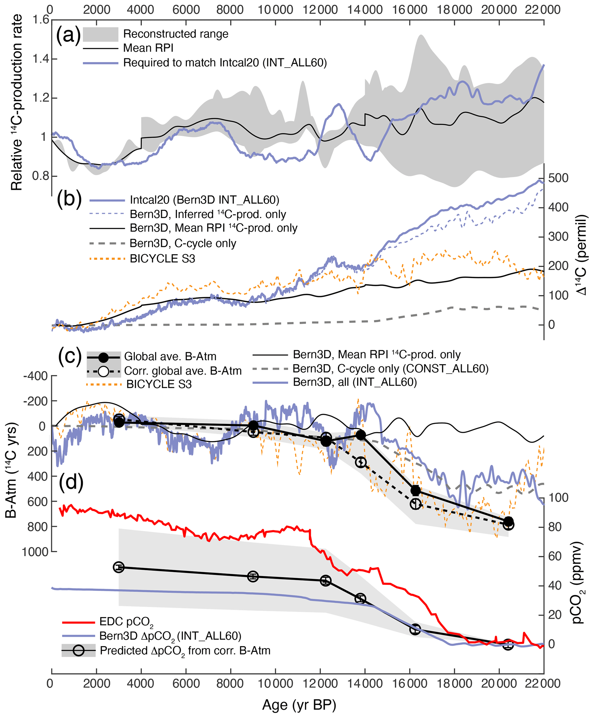
Figure 12Observed and modelled atmospheric and marine radiocarbon, compared with radiocarbon production rates, and atmospheric CO2. Panel (a)shows relative radiocarbon production rates. Shaded area: full range of reconstructed values (Laj et al., 2000, 2004; Adolphi et al., 2018; Channell et al., 2018; Nowaczyk et al., 2013); solid black line: mean RPI (Laj et al., 2000, 2004; Channell et al., 2018; Nowaczyk et al., 2013); thick blue line: as inferred from an idealized model scenario to match Intcal20, INT_ALL60 (1 kyr moving average; this study). Panel (b)shows atmospheric Δ14C anomalies normalized to modern values: prescribed in the INT_ALL60 model scenario (i.e. Intcal20, Reimer et al., 2020; solid dark blue line; this study); driven only by inferred production rates that match Intcal20 (INT_ALL60-CONST_ALL60; dashed blue line; this study); driven only by mean RPI production rates (solid black line; Dinauer et al., 2020); driven only by carbon cycle and ventilation changes in the CONST-ALL60 model scenario (dashed grey line; this study); simulated with the BICYCLE box model (Köhler et al., 2006) using 10Be-based (Muscheler et al., 2005) radiocarbon production estimates and a full carbon cycle scenario (dashed orange line). Panel (c) shows B-Atm radiocarbon age offset anomalies relative to modern values: Bern3D and BICYCLE model outputs as for (b); and inferred from time-slice interpolations (filled black circles and line; this study), including a maximal correction for “attenuation biases” (open black circles and dashed line), with the full range of reconstructed values (shaded area) due to uncertainties, corrections, and alternative data flagging scenarios (see Table 1). Panel (d)shows atmospheric CO2 normalized to LGM values: from EDC (red line; Monnin et al., 2001); inferred from observed mean “corrected” ocean B-Atm using a sensitivity of ∼ ppm per 100 14C yr (open black circles and line with shaded range; this study); and simulated in the Bern3D model for the INT_ALL60 scenario that is also illustrated in (a)–(c).
Model simulations of deglacial radiocarbon production and atmospheric radiocarbon and pCO2 consistently indicate that past Δ14Catm cannot be accounted for by existing reconstructions of changing radiocarbon production alone (e.g. Hain et al., 2014; Köhler et al., 2006; Dinauer et al., 2020; Köhler et al., 2022). Earth system model simulations applying mean relative palaeomagnetic intensity- (RPI) based radiocarbon production rate changes (Dinauer et al., 2020), yield only a small increase (∼ 150 ‰) in Δ14Catm at the LGM relative to the late Holocene (Fig. 12b, black line). Similar Δ14Catm changes are obtained using alternative radiocarbon production histories (Hain et al., 2014; Köhler et al., 2006; Dinauer et al., 2020; Köhler et al., 2022). The widely recognized implication of these results is that additional carbon cycle changes (i.e. altered rates of carbon exchange with other reservoirs) and/or different radiocarbon production changes are required in order to account for the observed Δ14Catm amplitude.
Turning to carbon cycle changes first, given the tight coupling of the marine and atmospheric carbon pools, altered exchange rates between the ocean and atmosphere are likely to have played a leading role in deglacial Δ14Catm variability (Muscheler et al., 2004). Arguably for the first time, our global average B-Atm estimates confirm such a role. Indeed, our mean ocean B-Atm estimates indicate a lower average exchange rate of radiocarbon (and likely CO2) between the ocean and atmosphere during the last glacial period, and an increase in this exchange rate across the deglaciation (Fig. 12c, black line and circles). All else being equal, an increase in ocean–atmosphere radiocarbon exchange would result in a drop in Δ14Catm during deglaciation, in parallel with a decrease in marine B-Atm offsets, as observed in Fig. 12b and c. Such changes would have also contributed to deglacial atmospheric CO2 rise (e.g. Muglia et al., 2018; Khatiwala et al., 2019; Brovkin et al., 2012; Ganopolski and Brovkin, 2017). As discussed above, a tentative quantification of this contribution to atmospheric CO2 rise can be derived from the observed mean ocean B-Atm (Table 1) and modelled sensitivities (Fig. 11a), as illustrated in Fig. 12d (open circles and shaded region). This tentative contribution compares well with simulated CO2 effects in the Bern3D model (INT_ALL60), bearing in mind that the simulated ageing of the global ocean is only ∼ 50 % of that observed (Fig. 12c, blue line and dashed grey line) and that ∼ 50 % of the simulated CO2 signal derives from ocean ventilation impacts alone.
While the observed mean ocean B-Atm estimates suggest a significant impact on the carbon cycle, the observed changes are still too small to account for the observed ∼ 400 ‰ drop in Δ14Catm across the deglaciation. This is demonstrated by model simulations that produce a mean ocean ageing of ∼ 500 14C yr (∼ 63 % of the observed value; Table 1) and yield a Δ14Catm increase of only ∼ 56 ‰, or ∼ 14 % of observed (Fig. 12b, dashed grey line). Similar results have been obtained using the BICYCLE box model (Köhler et al., 2006), which produced a Δ14Catm increase of only ∼ 200 ‰ at the LGM (∼ 50 % of observed), despite yielding mean ocean B-Atm offsets that match our observed values (Fig. 12b, c, dashed orange line). A mismatch was also obtained for the LGM using the CLIMBER intermediate complexity model (Ganopolski and Brovkin, 2017), where a 20 % higher radiocarbon production rate, combined with reduced ocean ventilation causing a global mean B-Atm increase of ∼ 800 years (again in line with our LGM estimate), coincided with a Δ14Catm increase of only ∼ 280 ‰ (∼ 70 % of observed).
Therefore, existing radiocarbon production records cannot account for past atmospheric radiocarbon variability, either alone or in conjunction with ocean ventilation changes that are consistent with global mean B-Atm estimates (Fig. 12b, c). While there remain uncertainties in atmospheric radiocarbon reconstructions, these are likely on the order of ∼ 1 % (Reimer et al., 2020), and it seems highly unlikely that Δ14Catm variability over the last glacial cycle has been significantly overestimated. Similarly, it seems implausible (though clearly not impossible) that existing marine radiocarbon data significantly underestimate the magnitude of mean ocean B-Atm change since the last glacial period. The problem of closing the global radiocarbon budget since the last glacial period becomes even more difficult if volcanic/metamorphic CO2 inputs are invoked as a significant contributor to the global carbon pool during the last glacial period (Stott et al., 2019, 2009) or if no change in ocean ventilation is inferred (Stott et al., 2021).
Given the wide range of existing radiocarbon production estimates (e.g. as compiled by Dinauer et al., 2020; Fig. 12a, shaded area), it seems reasonable to postulate that existing production reconstructions might, on average, underestimate the amplitude of radiocarbon production rate change between the last glacial and the late Holocene, as suggested by a recent box-model study (Köhler et al., 2022). A “polar bias” in radiocarbon production records derived from ice-core 10Be fluxes has indeed been recently quantified separately for the geomagnetic and heliomagnetic modulations of cosmogenic production (Adolphi et al., 2023). Nevertheless, it has also been noted that correcting for the identified long-term geomagnetic bias in 10Be would not eliminate the mismatch between observed and modelled Δ14Catm at the LGM (Adolphi et al., 2023). Our idealized simulations with prescribed Δ14Catm allow us to infer the radiocarbon production changes that would be needed to reconcile imposed ventilation and carbon cycle changes with observed atmospheric Δ14Catm (Fig. 12b, blue line. The rapid deglacial fluctuations in production that are inferred in this way (e.g. across HS1, the BA, and YD) almost certainly reflect biases due to transient carbon cycle and ocean ventilation changes that have not been implemented in our idealized simulations (see Sect. 2.5). However, the longer-term trend in inferred production rates indicates levels at the LGM that are close to the high end of the existing range of estimates (Fig. 12a, shaded area). A similar result has recently been obtained using the BICYCLE box model (Köhler et al., 2022). The higher radiocarbon production rates that are inferred at the LGM would have had a significant impact, possibly accounting for the majority of the deglacial atmospheric radiocarbon signal (Fig. 12b, dashed blue line). The implication of these results is that a parallel closure of the radiocarbon and carbon cycles since the last glacial period might yet be obtained by exploiting the plausible range of reconstructed radiocarbon production rates (Köhler et al., 2022). Our global average B-Atm estimates provide a useful new constraint for achieving this goal.
We present spatial interpolations of compiled radiocarbon data for a suite of time slices spanning the last deglaciation. The primary purpose of these interpolations is to derive global average B-Atm estimates. A clear trend in global average B-Atm offsets is apparent since the LGM (when B-Atm was ∼ 760 14C yr higher than today on average), demonstrating unambiguous changes in the partitioning of radiocarbon between the ocean and atmosphere across the last deglaciation.
The spatial interpolations cohere with previous studies in indicating a stepwise and spatially heterogeneous rejuvenation of the ocean interior across the last deglaciation, and in suggesting the operation of a “ventilation seesaw” between the North Atlantic and both the North Pacific and Southern Ocean, especially during HS1 the YD.
A comparison of surface-, shallow-, and deep-water B-Atm trends indicates that transport changes in the upper ocean across the last deglaciation were likely modest (Marchal and Zhao, 2021a) and that B-Atm changes in the upper ocean (< 2 km) were more strongly influenced by gas-exchange efficiency changes at high latitudes. In contrast, a more significant contribution from transport and/or water mass geometry is apparent in the deeper ocean (> 2 km).
The time-slice reconstructions emphasize a widespread drop in B-Atm at the onset of the BA, resulting in a global average B-Atm within ∼ 100 14C yr of modern global average. However, model sensitivity tests indicate that a portion of this B-Atm drop could have resulted from atmospheric radiocarbon dynamics that were independent of ocean ventilation (radiocarbon production, terrestrial carbon release, etc.). The exact magnitude of this effect cannot yet be quantified, but a maximum bias of ∼ −190 14C yr relative to the LGM is estimated. Such a bias would imply that mean ocean B-Atm at the BA underestimates the true “ventilation age” of the ocean.
Model sensitivity tests further suggest a direct relationship between global average B-Atm anomalies and atmospheric CO2 change, with a tentative average sensitivity of ∼ −6.3 ppm CO2 per 100 14C yr. On this basis, our global average B-Atm estimates would imply a non-negligible contribution to atmospheric CO2 change across the last deglaciation (perhaps as much as > 30 % of the total observed). Global average B-Atm estimates also suggest that any ventilation contribution to atmospheric CO2 change was concentrated during HS1, the BA, and the YD, and was largely exhausted by the onset of the Holocene.
While our results serve to underline, and tentatively to quantify, the ocean's role in deglacial carbon cycle change, they also demonstrate that a complete closure and reconciliation of the radiocarbon and carbon cycles since the last glacial remains to be achieved. Our results point to the possibility that, on average, existing reconstructions may tend to underestimate radiocarbon production rates during the last glacial period. Further work to improve the accuracy of past radiocarbon production rate estimates therefore emerges as a priority.
Data lodged with PANGAEA include the compiled radiocarbon data and regional splines (https://doi.org/10.1594/PANGAEA.960693, Skinner et al., 2023a), netCDF files of zonally averaged time-slice interpolations (https://doi.pangaea.de/10.1594/PANGAEA.962525, Skinner et al., 2023b), and global average B-Atm estimates derived for each time slice from the global interpolations (https://doi.pangaea.de/10.1594/PANGAEA.962526, Skinner et al., 2023c).
Animation of zonal average time-slices spanning the last deglaciation, derived from global interpolations of compiled radiocarbon data (https://doi.org/10.5446/63113, Skinner, 2023).
The supplement related to this article is available online at: https://doi.org/10.5194/cp-19-2177-2023-supplement.
LS designed the study, compiled and processed the radiocarbon data, and performed the interpolations with the assistance of FP. FP developed the interpolation code, and LS and FP analysed the interpolation outputs. Numerical model runs using Bern3D were performed by AJT and analysed by AJT, FJ, and LS. LS wrote the manuscript with input from all co-authors.
The contact author has declared that none of the authors has any competing interests.
Publisher’s note: Copernicus Publications remains neutral with regard to jurisdictional claims made in the text, published maps, institutional affiliations, or any other geographical representation in this paper. While Copernicus Publications makes every effort to include appropriate place names, the final responsibility lies with the authors.
This work benefited from discussions during the INQUA IPODS working group meeting held in Cambridge, UK, in 2018. Luke Skinner acknowledges support from the Royal Society, the Cambridge Isaac Newton Trust, and the NERC OCEAN-14 and ROGUE-14 projects. Aurich Jeltsch-Thömmes and Fortunat Joos acknowledge funding from the Swiss National Science Foundation. The authors are particularly grateful to Laurie Menviel for assistance with accessing the LOVECLIM results used to test the interpolation method, as well as Patrick Rafter, Ning Zhao, Dan Amrhein, and Olivier Marchal for helpful discussions. This study was initiated in 2019 and initially submitted for review in 2021, and we are grateful for the constructive comments of one anonymous reviewer at that stage and the comments of Juan Muglia and an anonymous reviewer at a later stage, all of which helped to improve the manuscript.
This research has been supported by the Natural Environment Research Council (grant no. NE/L006421/1), the Schweizerischer Nationalfonds zur Förderung der Wissenschaftlichen Forschung (grant no. SNF 200020_200511) and NERC (grant no. NE/V011464/1).
This paper was edited by Qiuzhen Yin and reviewed by Juan Muglia and one anonymous referee.
Adkins, J. F. and Boyle, E. A.: Changing atmospheric Δ14C and the record of deep water paleoventilation ages, Paleoceanography, 12, 337–344, 1997.
Adolphi, F., Herbst, K., Nilsson, A., and Panovska, S.: On the Polar Bias in Ice Core 10Be Data, J. Geophys. Res.-Atmos., 128, e2022JD038203, https://doi.org/10.1029/2022JD038203, 2023.
Adolphi, F., Bronk Ramsey, C., Erhardt, T., Edwards, R. L., Cheng, H., Turney, C. S. M., Cooper, A., Svensson, A., Rasmussen, S. O., Fischer, H., and Muscheler, R.: Connecting the Greenland ice-core and U Th timescales via cosmogenic radionuclides: testing the synchroneity of Dansgaard–Oeschger events, Clim. Past, 14, 1755–1781, https://doi.org/10.5194/cp-14-1755-2018, 2018.
Ahagon, N., Ohkushi, K., Uchida, M., and Mishima, T.: Mid-depth circulation in the northwest Pacific during the last deglaciation: Evidence from foraminferal radiocarbon ages, Geophys. Res. Lett., 30, 2.1–2.4, 2003.
Ausín, B., Sarnthein, M., and Haghipour, N.: Glacial-to-deglacial reservoir and ventilation ages on the southwest Iberian continental margin, Quaternary Sci. Rev., 255, 106818, https://doi.org/10.1016/j.quascirev.2021.106818, 2021.
Austin, W. E. N., Telford, R. J., Ninnemann, U. S., Brown, L., Wilson, L. J., Small, D. P., and Bryant, C. L.: North Atlantic reservoir ages linked to high Younger Dryas atmospheric radiocarbon concentrations, Global Planet. Change, 79, 226–233, https://doi.org/10.1016/j.gloplacha.2011.06.011, 2011.
Bard, E.: Correction of accelerator mass spectrometry 14C ages measured in planktonic foraminifera: Paleoceanographic implications, Paleoceanography, 3, 635–645, 1988.
Bard, E.: Geochemical and geophysical implications of the radiocarbon calibration, Geochim. Cosmochim. Ac., 62, 2025–2038, 1998.
Bard, E. and Heaton, T. J.: On the tuning of plateaus in atmospheric and oceanic 14C records to derive calendar chronologies of deep-sea cores and records of 14C marine reservoir age changes, Clim. Past, 17, 1701–1725, https://doi.org/10.5194/cp-17-1701-2021, 2021.
Bard, E., Arnold, M., Duprat, J., Moyes, J., and Duplessy, J.-C.: Reconstruction of the last deglaciation: deconvolved records of δ18O profiles, micropalaeontological variations and accelerator mass spectrometric 14C dating, Clim. Dynam., 1, 101–112, 1987.
Barker, S., Knorr, G., Vautravers, M., Diz, P., and Skinner, L. C.: Extreme deepening of the Atlantic overturning circulation during deglaciation, Nat. Geosci., 3, 567–571, https://doi.org/10.1038/NGEO921, 2010.
Barker, S., Knorr, G., Conn, S., Lordsmith, S., Newman, D., and Thornalley, D.: Early Interglacial Legacy of Deglacial Climate Instability, Paleoceanogr. Paleocl., 34, 1455–1475, https://doi.org/10.1029/2019pa003661, 2019.
Bova, S. C., Herbert, T. D., and Altabet, M. A.: Ventilation of Northern and Southern Sources of Aged Carbon in the Eastern Equatorial Pacific During the Younger Dryas Rise in Atmospheric CO2, Paleoceanogr. Paleocl., 33, 1151–1168, https://doi.org/10.1029/2018pa003386, 2018.
Bradtmiller, L. I., McManus, J. F., and Robinson, L. F.: 231Pa 230Th evidence for a weakened but persistent Atlantic meridional overturning circulation during Heinrich Stadial 1, Nat. Commun., 5, 5817, https://doi.org/10.1038/ncomms6817, 2014.
Broecker, W. and Barker, S.: A 190 permil drop in atmosphere's Δ14C during the “Mystery Interval” (17.5 to 14.5 kyr), Earth Planet. Sc. Lett., 256, 90–99, 2007.
Broecker, W. and Clark, E.: Is the magnitude of the carbonate ion decrease in the abyssal ocean over the last 8 kyr consistent with the 20 ppm rise in atmospheric CO2 content, Paleoceanography, 22, 1–10, 2007.
Broecker, W. S.: Palaeocean circulation during the last deglaciation: a bipolar seesaw?, Paleoceanography, 13, 119–121, 1998.
Brovkin, V., Ganopolski, A., Archer, D., and Munhoven, G.: Glacial CO2 cycle as a succession of key physical and biogeochemical processes, Clim. Past, 8, 251–264, https://doi.org/10.5194/cp-8-251-2012, 2012.
Burke, A. and Robinson, L. F.: The Southern Ocean's role in carbon exchange during the last deglaciation, Science, 335, 557–561, 2012.
Channell, J. E. T., Hodell, D. A., Crowhurst, S. J., Skinner, L. C., and Muscheler, R.: Relative paleointensity (RPI) in the latest Pleistocene (10–45 ka) and implications for deglacial atmospheric radiocarbon, Quaternary Sci. Rev., 191, 57–72, https://doi.org/10.1016/j.quascirev.2018.05.007, 2018.
Chen, T., Robinson, L. F., Burke, A., Southon, J., Spooner, P., Morris, P. J., and Ng, H. C.: Synchronous centennial abrupt events in the ocean and atmosphere during the last deglaciation, Science, 349, 1537–1541, https://doi.org/10.1126/science.aac6159, 2015.
Cook, M. and Keigwin, L. D.: Radiocarbon profiles of the NW Pacific from the LGM and deglaciation: Evaluating ventilation metrics and the effect of uncertain surface reservoir ages, Paleoceanography, 30, 174–195, https://doi.org/10.1002/2014PA002649, 2015.
Dinauer, A., Adolphi, F., and Joos, F.: Mysteriously high Δ14C of the glacial atmosphere: influence of 14C production and carbon cycle changes, Clim. Past, 16, 1159–1185, https://doi.org/10.5194/cp-16-1159-2020, 2020.
Dolman, A. M., Groeneveld, J., Mollenhauer, G., Ho, S. L., and Laepple, T.: Estimating bioturbation from replicated small-sample radiocarbon ages, Paleoceanogr. Paleocl., 36, e2020PA004142, https://doi.org/10.1029/2020PA004142, 2021.
Edwards, N. R., Willmott, A. J., and Killworth, P. D.: On the Role of Topography and Wind Stress on the Stability of the Thermohaline Circulation, J. Phys. Oceanogr., 28, 756–778, https://doi.org/10.1175/1520-0485(1998)028<0756:otrota>2.0.co;2, 1998.
Eggleston, S. and Galbraith, E. D.: The devil's in the disequilibrium: multi-component analysis of dissolved carbon and oxygen changes under a broad range of forcings in a general circulation model, Biogeosciences, 15, 3761–3777, https://doi.org/10.5194/bg-15-3761-2018, 2018.
England, M. H.: The Age of Water and Ventilation Timescales in a Global Ocean Model, J. Phys. Oceanogr., 25, 2756-2777, https://doi.org/10.1175/1520-0485(1995)025<2756:TAOWAV>2.0.CO;2, 1995.
EPICA community members: Eight glacial cycles from an Antarctic ice core, Nature, 429, 623–628, 2004.
EPICA community members: One-to-one coupling of glacial variability in Greenland and Antarctica, Nature, 444, 195–198, 2006.
Ferrari, R., Jansen, M. F., Adkins, J. F., Burke, A., Stewart, A. L., and Thompson, A. F.: Antarctic sea ice control on ocean circulation in present and glacial climates, P. Natl. Acad. Sci. USA, 111, 8753–8758, https://doi.org/10.1073/pnas.1323922111, 2014.
Franke, J., Paul, A., and Schulz, M.: Modeling variations of marine reservoir ages during the last 45 000 years, Clim. Past, 4, 125–136, https://doi.org/10.5194/cp-4-125-2008, 2008.
Freeman, E., Skinner, L. C., Tisserand, A., Dokken, T., Timmermann, A., Menviel, L., and Friedrich, T.: An Atlantic-Pacific ventilation seesaw across the last deglaciation, Earth Planet. Sc. Lett., 424, 237–244, https://doi.org/10.1016/j.epsl.2015.05.032, 2015.
Galbraith, E., Kwon, E. Y., Bianchi, D., Hain, M. P., and Sarmiento, J. L.: The impact of atmospheric pCO2 on carbon isotope ratios of the atmosphere and ocean, Global Biogeochem. Cy., 29, 307–324, https://doi.org/10.1002/2014GB004929, 2015.
Galbraith, E. D. and Skinner, L. C.: The Biological Pump During the Last Glacial Maximum, Annu. Rev. Mar. Sci., 12, 559–586, https://doi.org/10.1146/annurev-marine-010419-010906, 2020.
Ganopolski, A. and Brovkin, V.: Simulation of climate, ice sheets and CO2 evolution during the last four glacial cycles with an Earth system model of intermediate complexity, Clim. Past, 13, 1695–1716, https://doi.org/10.5194/cp-13-1695-2017, 2017.
Gherardi, J.-M., Labeyrie, L., McManus, J. F., Francois, R., Skinner, L. C., and Cortijo, E.: Evidence from the North Eastern Atlantic Basin for Variability of the Meridional Overturning Circulation through the last Deglaciation, Earth Planet. Sc. Lett., 240, 710–723, 2005.
Gottschalk, J., Battaglia, G., Fischer, H., Frölicher, T. L., Jaccard, S. L., Jeltsch-Thömmes, A., Joos, F., Köhler, P., Meissner, K. J., Menviel, L., Nehrbass-Ahles, C., Schmitt, J., Schmittner, A., Skinner, L. C., and Stocker, T. F.: Mechanisms of millennial-scale atmospheric CO2 change in numerical model simulations, Quaternary Sci. Rev., 220, 30–74, https://doi.org/10.1016/j.quascirev.2019.05.013, 2019.
Gottschalk, J., Michel, E., Thöle, L. M., Studer, A. S., Hasenfratz, A. P., Schmid, N., Butzin, M., Mazaud, A., Martínez-García, A., Szidat, S., and Jaccard, S. L.: Glacial heterogeneity in Southern Ocean carbon storage abated by fast South Indian deglacial carbon release, Nat. Commun., 11, 6192, https://doi.org/10.1038/s41467-020-20034-1, 2020.
Hain, M. P., Sigman, D. M., and Haug, G. H.: Distinct roles of the Southern Ocean and North Atlantic in the deglacial atmospheric radiocarbon decline, Earth Planet. Sc. Lett., 394, 198–208, https://doi.org/10.1016/j.epsl.2014.03.020, 2014.
Heaton, T. J., Bard, E., Bronk Ramsey, C., Butzin, M., Köhler, P., Muscheler, R., Reimer, P. J., and Wacker, L.: Radiocarbon: A key tracer for studying Earth's dynamo, climate system, carbon cycle, and Sun, Science, 374, eabd7096, https://doi.org/10.1126/science.abd7096, 2021.
Heaton, T. J., Köhler, P., Butzin, M., Bard, E., Reimer, R. W., Austin, W. E. N., Bronk Ramsey, C., Grootes, P. M., Hughen, K. A., Kromer, B., Reimer, P. J., Adkins, J., Burke, A., Cook, M. S., Olsen, J., and Skinner, L. C.: Marine20 – The Marine Radiocarbon Age Calibration Curve (0–55,000 cal BP), Radiocarbon, 62, 779–820, https://doi.org/10.1017/RDC.2020.68, 2020.
Hines, S. K. V., Southon, J. R., and Adkins, J. F.: A high-resolution record of Southern Ocean intermediate water radiocarbon over the past 30,000 years, Earth Planet. Sc. Lett., 432, 46–58, https://doi.org/10.1016/j.epsl.2015.09.038, 2015.
Hines, S. K. V., Thompson, A. F., and Adkins, J. F.: The Role of the Southern Ocean in Abrupt Transitions and Hysteresis in Glacial Ocean Circulation, Paleoceanogr. Paleocl., 34, 490–510, https://doi.org/10.1029/2018pa003415, 2019.
Jeltsch-Thömmes, A. and Joos, F.: Modeling the evolution of pulse-like perturbations in atmospheric carbon and carbon isotopes: the role of weathering–sedimentation imbalances, Clim. Past, 16, 423–451, https://doi.org/10.5194/cp-16-423-2020, 2020.
Jeltsch-Thömmes, A., Battaglia, G., Cartapanis, O., Jaccard, S. L., and Joos, F.: Low terrestrial carbon storage at the Last Glacial Maximum: constraints from multi-proxy data, Clim. Past, 15, 849–879, https://doi.org/10.5194/cp-15-849-2019, 2019.
Jochum, M., Chase, Z., Nuterman, R., Pedro, J., Rasmussen, S., Vettoretti, G., and Zheng, P.: Carbon Fluxes during Dansgaard–Oeschger Events as Simulated by an Earth System Model, J. Climate, 35, 5745–5758, https://doi.org/10.1175/jcli-d-21-0713.1, 2022.
Joos, F., Gerber, S., Prentice, I. C., Otto-Bliesner, B. L., and Valdes, P. J.: Transient simulations of Holocene atmospheric carbon dioxide and terrestrial carbon since the Last Glacial Maximum, Global Biogeochem. Cy., 18, GB2002, https://doi.org/10.1029/2003gb002156, 2004.
Key, R. M., Kozyr, A., Sabine, C., Lee, K., Wanninkhof, R., Bullister, J. L., Feely, R. A., Millero, F. J., Mordy, C., and Peng, T.-H.: A global ocean carbon climatology: Results from the Global Data Analysis Project (GLODAP), Global Biogeochem. Cy., 18, 1–23, 2004.
Khatiwala, S., Muglia, J., and Schmittner, A.: Air-sea disequilibrium enhances ocean carbon storage during glacial periods, Science Advances, 5, 1–10, 2019.
Koeve, W., Wagner, H., Kähler, P., and Oschlies, A.: 14C-age tracers in global ocean circulation models, Geosci. Model Dev., 8, 2079–2094, https://doi.org/10.5194/gmd-8-2079-2015, 2015.
Köhler, P., Muscheler, R., and Fischer, H.: A model-based interpre- tation of low-frequency changes in the carbon cycle during the last 120,000 years and its implications for the reconstruction of atmospheric Δ14C, Geochem. Geophy. Geosy., 7, 1–22, 2006.
Köhler, P., Knorr, G., and Bard, E.: Permafrost thawing as a possible source of abrupt carbon release at the onset of the Bølling/Allerød, Nat. Commun., 5, 5520, https://doi.org/10.1038/ncomms6520, 2014.
Köhler, P., Adolphi, F., Butzin, M., and Muscheler, R.: Toward Reconciling Radiocarbon Production Rates With Carbon Cycle Changes of the Last 55,000 Years, Paleoceanogr. Paleocl., 37, e2021PA004314, https://doi.org/10.1029/2021PA004314, 2022.
Kwon, E. Y., Sarmiento, J. L., Toggweiler, J. R., and DeVries, T.: The control of atmospheric pCO2 by ocean ventilation change: The effect of the oceanic storage of biogenic carbon, Global Biogeochem. Cy., 25, GB3026, https://doi.org/10.1029/2011GB004059, 2011.
Laj, C., Kissel, C., Mazaud, A., Channell, J. E. T., and Beer, J.: North Atlantic palaeointensity stack since 75 ka (NAPIS–75) and the duration of the Laschamp event, Philos. T. R. Soc. A, 358, 1009–1025, https://doi.org/10.1098/rsta.2000.0571, 2000.
Laj, C., Kissel, C., and Beer, J.: High resolution global paleointensity stack since 75 kyr (GLOPIS-75) calibrated to absolute values, in: Timescales of the Paleomagnetic Field, Geophysical Monograph Series, American Geophysical Union, 145, 255–265, 2004.
Leduc, G., Vidal, L., Tachikawa, K., Rostek, F., Sonzogni, C., Beaufort, L., and Bard, E.: Moisture transport across Central America as a positive feedback on abrupt climatic changes, Nature, 445, 908, https://doi.org/10.1038/nature05578, 2007.
Lemieux-Dudon, B., Blayo, E., Petit, J. R., Waelbroeck, C., Svensson, A., Ritz, C., Barnola, J.-M., Narcisi, B. M., and Parrenin, F.: Consistent dating for Antactic and Greenland ice cores, Quaternary Sci. Rev., 29, 8–20, 2010.
Lindsay, C. M., Lehman, S. J., Marchitto, T. M., and Ortiz, J. D.: The surface expression of radiocarbon anomalies near Baja California during deglaciation, Earth Planet. Sc. Lett., 422, 67–74, https://doi.org/10.1016/j.epsl.2015.04.012, 2015.
Lindsay, C. M., Lehman, S. J., Marchitto, T. M., Carriquiry, J. D., and Ortiz, J. D.: New constraints on deglacial marine radiocarbon anomalies from a depth transect near Baja California, Paleoceanography, 31, 1103–1116, https://doi.org/10.1002/2015pa002878, 2016.
Lougheed, B. C., Ascough, P., Dolman, A. M., Löwemark, L., and Metcalfe, B.: Re-evaluating 14C dating accuracy in deep-sea sediment archives, Geochronology, 2, 17–31, https://doi.org/10.5194/gchron-2-17-2020, 2020.
Lund, D. C., Tessin, A. C., Hoffman, J. L., and Schmittner, A.: Southwest Atlantic water mass evolution during the last deglaciation, Paleoceanography, 30, 477-494, https://doi.org/10.1002/2014PA002657, 2015.
Maier-Reimer, E. and Hasselmann, K.: Transport and storage of CO2 in the ocean – an inorganic ocean-circulation carbon cycle model, Clim. Dynam., 2, 63–90, https://doi.org/10.1007/BF01054491, 1987.
Marchal, O. and Zhao, N.: On the Estimation of Deep Atlantic Ventilation from Fossil Radiocarbon Records. Part II: (In)consistency with Modern Estimates, J. Phys. Oceanogr., 51, 2681–2704, https://doi.org/10.1175/JPO-D-20-0314.1, 2021a.
Marchal, O. and Zhao, N.: On the estimation of deep Atlantic ventilation from fossil radiocarbon records. Part I: Modern reference estimates, J. Phys. Oceanogr., 51, 1843–1873, https://doi.org/10.1175/JPO-D-20-0153.1, 2021b.
Marchal, O., Stocker, T. F., and Joos, F.: Impact of oceanic reorganisations on the ocean carbon cycle and atmospheric carbon dioxide content, Paleoceanography, 13, 225–244, 1998.
Marchitto, T. M., Lehman, S. J., Otiz, J. D., Flückiger, J., and van Geen, A.: Marine radiocarbon evidence for the mechanism of deglacial atmospheric CO2 rise, Science, 316, 1456–1459, 2007.
Marcott, S. A., Bauska, T. K., Buizert, C., Steig, E. J., Rosen, J. L., Cuffey, K. M., Fudge, T. J., Severinghaus, J. P., Ahn, J., Kalk, M. L., McConnell, J. R., Sowers, T., Taylor, K. C., White, J. W. C., and Brook, E. J.: Centennial-scale changes in the global carbon cycle during the last deglaciation, Nature, 514, 616–619, https://doi.org/10.1038/nature13799, 2014.
Matsumoto, K.: Radiocarbon-based circulation age of the world oceans, J. Geophys. Res., 112, C09004, https://doi.org/10.1029/2007JC004095, 2007.
Max, L., Lembke-Jene, L., Riethdorf, J.-R., Tiedemann, R., Nürnberg, D., Kühn, H., and Mackensen, A.: Pulses of enhanced North Pacific Intermediate Water ventilation from the Okhotsk Sea and Bering Sea during the last deglaciation, Clim. Past, 10, 591–605, https://doi.org/10.5194/cp-10-591-2014, 2014.
McClelland, H. L. O., Halevy, I., Wolf-Gladrow, D. A., Evans, D., and Bradley, A. S.: Statistical Uncertainty in Paleoclimate Proxy Reconstructions, Geophys. Res. Lett., 48, e2021GL092773, https://doi.org/10.1029/2021GL092773, 2021.
McManus, J. F., Francois, R., Gherardi, J.-M., Keigwin, L. D., and Brown-Leger, S.: Collapse and rapid resumption of the Atlantic meridional circulation linked to deglacial climate changes, Nature, 428, 834–837, 2004.
Menviel, L., Timmermann, A., Mouchet, A., and Timm, O.: Meridional reorganizations of marine and terrestrial productivity during Heinrich events, Paleoceanography, 23, PA1203, https://doi.org/10.1029/2007PA001445, 2008.
Menviel, L., Joos, F., and Ritz, S. P.: Simulating atmospheric CO2, 13C and the marine carbon cycle during the Last Glacial–Interglacial cycle: possible role for a deepening of the mean remineralization depth and an increase in the oceanic nutrient inventory, Quaternary Sci. Rev., 56, 46–68, https://doi.org/10.1016/j.quascirev.2012.09.012, 2012.
Menviel, L., England, M. H., Meissner, K. J., Mouchet, A., and Yu, J.: Atlantic-Pacific seesaw and its role in outgassing CO2 during Heinrich events, Paleoceanography, 29, 58–70, https://doi.org/10.1002/2013pa002542, 2014.
Menviel, L., Spence, P., and England, M. H.: Contribution of enhanced Antarctic Bottom Water formation to Antarctic warm events and millennial-scale atmospheric CO2 increase, Earth Planet. Sc. Lett., 413, 37–50, https://doi.org/10.1016/j.epsl.2014.12.050, 2015.
Menviel, L., Yu, J., Joos, F., Mouchet, A., Meissner, K. J., and England, M. H.: Poorly ventilated deep ocean at the Last Glacial Maximum inferred from carbon isotopes: A data-model comparison study, Paleoceanography, 32, 2–17, https://doi.org/10.1002/2016pa003024, 2017.
Menviel, L., Spence, P., Yu, J., Chamberlain, M. A., Matear, R. J., Meissner, K. J., and England, M. H.: Southern Hemisphere westerlies as a driver of the early deglacial atmospheric CO2 rise, Nat. Commun., 9, 2503, https://doi.org/10.1038/s41467-018-04876-4, 2018.
Missiaen, L., Wacker, L., Lougheed, B. C., Skinner, L., Hajdas, I., Nouet, J., Pichat, S., and Waelbroeck, C.: Radiocarbon Dating of Small-sized Foraminifer Samples: Insights into Marine sediment Mixing, Radiocarbon, 62, 313–333, https://doi.org/10.1017/RDC.2020.13, 2020.
Monnin, E., Indermuhle, A., Dallenbach, A., Fluckiger, J., Stauffer, B., Stocker, T. F., Raynaud, D., and Barnola, J. M.: Atmospheric CO2 Concentrations over the Last Glacial Termination, Science, 291, 112–114, 2001.
Muglia, J. and Schmittner, A.: Carbon isotope constraints on glacial Atlantic meridional overturning: Strength vs depth, Quaternary Sci. Rev., 257, 106844, https://doi.org/10.1016/j.quascirev.2021.106844, 2021.
Muglia, J., Skinner, L. C., and Schmittner, A.: Weak overturning circulation and high Southern Ocean nutrient utilization maximized glacial ocean carbon, Earth Planet. Sc. Lett., 496, 47–56, https://doi.org/10.1016/j.epsl.2018.05.038, 2018.
Müller, S. A., Joos, F., Edwards, N. R., and Stocker, T. F.: Water mass distribution and ventilation time scales in a cost-efficient, three-dimensional ocena model, J. Climate, 19, 5479–5499, 2006.
Müller, S. A., Joos, F., Plattner, G. K., Edwards, N. R., and Stocker, T. F.: Modeled natural and excess radiocarbon: Sensitivities to the gas exchange formulation and ocean transport strength, Global Biogeochem. Cy., 22, Gb3011, https://doi.org/10.1029/2007gb003065, 2008.
Muscheler, R., Beer, J., Wagner, G., Laj, C., Kissel, C., Raisbeck, G. M., Yiou, F., and Kubik, P. W.: Changes in the carbon cycle during the last deglaciation as indicated by the comparison of 10Be and 14C records, Earth Planet. Sc. Lett., 219, 325–340, 2004.
Muscheler, R., Beer, J., Kubik, P. W., and Synal, H.-A.: Geomagnetic field intensity during the last 60,000 years based on 10Be and 36Cl from the Summit ice cores and 14C, Quaternary Sci. Rev., 24, 1846–1860, 2005.
Muschitiello, F., D'Andrea, W. J., Schmittner, A., Heaton, T. J., Balascio, N. L., deRoberts, N., Caffee, M. W., Woodruff, T. E., Welten, K. C., Skinner, L. C., Simon, M. H., and Dokken, T. M.: Deep-water circulation changes lead North Atlantic climate during deglaciation, Nat. Commun., 10, 1272, https://doi.org/10.1038/s41467-019-09237-3, 2019.
Ng, H. C., Robinson, L. F., McManus, J. F., Mohamed, K. J., Jacobel, A. W., Ivanovic, R. F., Gregoire, L. J., and Chen, T.: Coherent deglacial changes in western Atlantic Ocean circulation, Nat. Commun., 9, 2947, https://doi.org/10.1038/s41467-018-05312-3, 2018.
Nowaczyk, N. R., Frank, U., Kind, J., and Arz, H. W.: A high-resolution paleointensity stack of the past 14 to 68 ka from Black Sea sediments, Earth Planet. Sc. Lett., 384, 1–16, https://doi.org/10.1016/j.epsl.2013.09.028, 2013.
Okazaki, Y., Timmermann, A., Menviel, L., Harada, N., Abe-Ouchi, A., Chikamoto, M. O., Mouchet, A., and Asahi, H.: Deepwater Formation in the North Pacific During the Last Glacial Termination, Science, 329, 200–204, https://doi.org/10.1126/science.1190612, 2010.
Parnell, A. C., Haslett, J., Allen, J. R. M., Buck, C. E., and Huntley, B.: A flexible approach to assessing synchroneity of past events using Bayesian reconstructions of sedimentation history, Quaternary Sci. Rev., 27, 1872–1855, 2008.
Peck, V. L., Hall, I. R., Zahn, R., Elderfield, H., Grousset, F., Hemming, S. R., and Scourse, J. D.: High resolution evidence for linkages between NW European ice sheet instability and Atlantic Meridional Overturning Circulation, Earth Planet. Sc. Lett., 243, 476–488, https://doi.org/10.1016/j.epsl.2005.12.023, 2006.
Pöppelmeier, F., Jeltsch-Thömmes, A., Lippold, J., Joos, F., and Stocker, T. F.: Multi-proxy constraints on Atlantic circulation dynamics since the last ice age, Nat. Geosci., 16, 349–356, https://doi.org/10.1038/s41561-023-01140-3, 2023.
Primeau, F.: Characterizing transport between the surface mixed layer and the ocean interior with a forward adjoint global ocean transport model, J. Phys. Oceanogr., 35, 545–564, 2005.
Rae, J. W. B., Burke, A., Robinson, L. F., Adkins, J. F., Chen, T., Cole, C., Greenop, R., Li, T., Littley, E. F. M., Nita, D. C., Stewart, J. A., and Taylor, B. J.: CO2 storage and release in the deep Southern Ocean on millennial to centennial timescales, Nature, 562, 569–573, https://doi.org/10.1038/s41586-018-0614-0, 2018.
Rafter, P. A., Herguera, J.-C., and Southon, J. R.: Extreme lowering of deglacial seawater radiocarbon recorded by both epifaunal and infaunal benthic foraminifera in a wood-dated sediment core, Clim. Past, 14, 1977–1989, https://doi.org/10.5194/cp-14-1977-2018, 2018.
Rafter, P. A., Carriquiry, J. D., Herguera, J.-C., Hain, M. P., Solomon, E. A., and Southon, J. R.: Anomalous > 2000-Year-Old Surface Ocean Radiocarbon Age as Evidence for Deglacial Geologic Carbon Release, Geophys. Res. Lett., 46, 13950–13960, https://doi.org/10.1029/2019gl085102, 2019.
Rafter, P. A., Gray, W. R., Hines, S. K. V., Burke, A., Costa, K. M., Gottschalk, J., Hain, M. P., Rae, J. W. B., Southon, J. R., Walczak, M. H., Yu, J., Adkins, J. F., and DeVries, T.: Global reorganization of deep-sea circulation and carbon storage after the last ice age, Science Advances, 8, eabq5434, https://doi.org/10.1126/sciadv.abq5434, 2022.
Rasmussen, S. O., Bigler, M., Blockley, S. P., Blunier, T., Buchardt, S. L., Clausen, H. B., Cvijanovic, I., Dahl-Jensen, D., Johnsen, S. J., Fischer, H., Gkinis, V., Guillevic, M., Hoek, W. Z., Lowe, J. J., Pedro, J. B., Popp, T., Seierstad, I. K., Steffensen, J. P., Svensson, A. M., Vallelonga, P., Vinther, B. M., Walker, M. J. C., Wheatley, J. J., and Winstrup, M.: A stratigraphic framework for abrupt climatic changes during the Last Glacial period based on three synchronized Greenland ice-core records: refining and extending the INTIMATE event stratigraphy, Quaternary Sci. Rev., 106, 14–28, https://doi.org/10.1016/j.quascirev.2014.09.007, 2014.
Reimer, P. J., Austin, W. E. N., Bard, E., Bayliss, A., Blackwell, P. G., Bronk Ramsey, C., Butzin, M., Cheng, H., Edwards, R. L., Friedrich, M., Grootes, P. M., Guilderson, T. P., Hajdas, I., Heaton, T. J., Hogg, A. G., Hughen, K. A., Kromer, B., Manning, S. W., Muscheler, R., Palmer, J. G., Pearson, C., van der Plicht, J., Reimer, R. W., Richards, D. A., Scott, E. M., Southon, J. R., Turney, C. S. M., Wacker, L., Adolphi, F., Büntgen, U., Capano, M., Fahrni, S. M., Fogtmann-Schulz, A., Friedrich, R., Köhler, P., Kudsk, S., Miyake, F., Olsen, J., Reinig, F., Sakamoto, M., Sookdeo, A., and Talamo, S.: The INTCAL20 Northern Hemisphere radiocarbon age calibration curve (0–55 cal kBP), Radiocarbon, 62, 725–757, https://doi.org/10.1017/RDC.2020.41, 2020.
Ritz, S. P., Stocker, T. F., and Joos, F.: A Coupled Dynamical Ocean–Energy Balance Atmosphere Model for Paleoclimate Studies, J. Climate, 24, 349–375, https://doi.org/10.1175/2010jcli3351.1, 2011.
Robinson, L. F., Adkins, J. F., Keigwin, L. D., Southon, J., Fernandez, D. P., Wang, S.-L., and Scheirer, D. S.: Radiocarbon variability in the western North Atlantic during the last deglaciation, Science, 310, 1469–1473, 2005.
Ronge, T. A., Tiedemann, R., Lamy, F., Köhler, P., Alloway, B.V., De Pol-Holz, R., Pahnke, K., Southon, J., and Wacker, L.: Radiocarbon constraints on the extent and evolution of the South Pacific glacial carbon pool, Nat. Commun., 7, 11487, https://doi.org/10.1038/ncomms11487, 2016.
Ronge, T. A., Sarnthein, M., Roberts, J., Lamy, F., and Tiedemann, R.: East Pacific Rise Core PS75/059-2: Glacial-to-Deglacial Stratigraphy Revisited, Paleoceanogr. Paleocl., 34, 432–435, https://doi.org/10.1029/2019PA003569, 2019.
Ronge, T. A., Prange, M., Mollenhauer, G., Ellinghausen, M., Kuhn, G., and Tiedemann, R.: Radiocarbon Evidence for the Contribution of the Southern Indian Ocean to the Evolution of Atmospheric CO2 Over the Last 32,000 Years, Paleoceanogr. Paleocl., 35, e2019PA003733, https://doi.org/10.1029/2019PA003733, 2020.
Rose, K. A., Sikes, E. L., Guilderson, T. P., Shane, P., Hill, T. M., Zahn, R., and Spero, H. J.: Upper-ocean-to-atmosphere radiocarbon offsets imply fast deglacial carbon dioxide release, Nature, 466, 1093–1097, 2010.
Roth, R., Ritz, S. P., and Joos, F.: Burial-nutrient feedbacks amplify the sensitivity of atmospheric carbon dioxide to changes in organic matter remineralisation, Earth Syst. Dynam., 5, 321–343, https://doi.org/10.5194/esd-5-321-2014, 2014.
Sarnthein, M., Schneider, B., and Grootes, P. M.: Peak glacial 14C ventilation ages suggest major draw-down of carbon into the abyssal ocean, Clim. Past, 9, 2595–2614, https://doi.org/10.5194/cp-9-2595-2013, 2013.
Sarnthein, M., Grootes, P. M., Kennett, J. P., and Nadeau, M.-J.: 14-C Reservoir ages show deglacial changes in ocean currents and carbon cycle, in: Ocean Circulation: Mechanisms and Impacts, edited by: Schmittner, A., Chiang, C. H., and Hemming, S. R., Geophysical Monographs, AGU, Washington DC, 173, 175–196, 2007.
Sarnthein, M., Balmer, S., Grootes, P., and Mudelsee, M.: Planktic and Benthic 14C Reservoir Ages for Three Ocean Basins, Calibrated by a Suite of 14C Plateaus in the Glacial-to-Deglacial Suigetsu Atmospheric 14C Record, Radiocarbon, 57, 129–151, https://doi.org/10.2458/azu_rc.57.17916, 2015.
Sarnthein, M., Küssner, K., Grootes, P. M., Ausin, B., Eglinton, T., Muglia, J., Muscheler, R., and Schlolaut, G.: Plateaus and jumps in the atmospheric radiocarbon record – potential origin and value as global age markers for glacial-to-deglacial paleoceanography, a synthesis, Clim. Past, 16, 2547–2571, https://doi.org/10.5194/cp-16-2547-2020, 2020.
Schüpbach, S., Fischer, H., Bigler, M., Erhardt, T., Gfeller, G., Leuenberger, D., Mini, O., Mulvaney, R., Abram, N. J., Fleet, L., Frey, M. M., Thomas, E., Svensson, A., Dahl-Jensen, D., Kettner, E., Kjaer, H., Seierstad, I., Steffensen, J. P., Rasmussen, S. O., Vallelonga, P., Winstrup, M., Wegner, A., Twarloh, B., Wolff, K., Schmidt, K., Goto-Azuma, K., Kuramoto, T., Hirabayashi, M., Uetake, J., Zheng, J., Bourgeois, J., Fisher, D., Zhiheng, D., Xiao, C., Legrand, M., Spolaor, A., Gabrieli, J., Barbante, C., Kang, J. H., Hur, S. D., Hong, S. B., Hwang, H. J., Hong, S., Hansson, M., Iizuka, Y., Oyabu, I., Muscheler, R., Adolphi, F., Maselli, O., McConnell, J., and Wolff, E. W.: Greenland records of aerosol source and atmospheric lifetime changes from the Eemian to the Holocene, Nat. Commun., 9, 1476, https://doi.org/10.1038/s41467-018-03924-3, 2018.
Siegenthaler, U.: Carbon-14 in the oceans, in: Handbook of Environmental Isotope Geochemistry, edited by: Fritz, P., and Fontes, J. C., Elsevier, Amsterdam, ISBN 0-444-42764-3, 1989.
Siegenthaler, U. and Oeschger, H.: Biospheric CO2 emissions during the past 200 years reconstructed by deconvolution of ice core data, Tellus B, 39, 140–154, https://doi.org/10.3402/tellusb.v39i1-2.15331, 1987.
Siegenthaler, U., Heimann, M., and Oeschger, H.: 14C variations caused by changes in the global carbon cycle, Radiocarbon, 22, 177–191, 1980.
Sikes, E. L., Cook, M. S., and Guilderson, T. P.: Reduced deep ocean ventilation in the Southern Pacific Ocean during the last glaciation persisted into the deglaciation, Earth Planet. Sc. Lett., 438, 130–138, https://doi.org/10.1016/j.epsl.2015.12.039, 2016a.
Sikes, E. L., Elmore, A. C., Allen, K. A., Cook, M. S., and Guilderson, T. P.: Glacial water mass structure and rapid δ18O and δ13C changes during the last glacial termination in the Southwest Pacific, Earth Planet. Sc. Lett., 456, 87–97, https://doi.org/10.1016/j.epsl.2016.09.043, 2016b.
Skinner, L.: Deglacial marine radiocarbon time-slice animation, TIB AV-Portal [video], https://doi.org/10.5446/63113, 2023.
Skinner, L. C. and Bard, E.: Radiocarbon as a Dating Tool and Tracer in Paleoceanography, Rev. Geophys., 60, e2020RG000720, https://doi.org/10.1029/2020RG000720, 2022.
Skinner, L., Muschitiello, F., and Scrivner, A. E.: Marine Reservoir Age Variability Over the Last Deglaciation: Implications for Marine Carbon Cycling and Prospects for Regional Radiocarbon Calibrations, Paleoceanogr. Paleocl., 34, 1807–1815, https://doi.org/10.1029/2019pa003667, 2019.
Skinner, L., Menviel, L., Broadfield, L., Gottschalk, J., and Greaves, M.: Southern Ocean convection amplified past Antarctic warming and atmospheric CO2 rise during Heinrich Stadial 4, Commun. Earth Environ., 1, 23, https://doi.org/10.1038/s43247-020-00024-3, 2020.
Skinner, L., Freeman, E., Hodell, D., Waelbroeck, C., Vasquez Riveiros, N., and Scrivner, A.: Atlantic Ocean ventilation changes across the last deglaciation and their carbon cycle implications, Paleoceanogr. Paleocl., 36, e2020PA004074, https://doi.org/10.1029/2020PA004074, 2021.
Skinner, L. C., Fallon, S., Waelbroeck, C., Michel, E., and Barker, S.: Ventilation of the deep Southern Ocean and deglacial CO2 rise, Science, 328, 1147–1151, 2010.
Skinner, L. C., Scrivner, A., Vance, D., Barker, S., Fallon, S., and Waelbroeck, C.: North Atlantic versus Southern Ocean contributions to a deglacial surge in deep ocean ventilation, Geology, 41, 667–670, https://doi.org/10.1130/G34133.1 2013.
Skinner, L. C., Waelbroeck, C., Scrivner, A., and Fallon, S.: Radiocarbon evidence for alternating northern and southern sources of ventilation of the deep Atlantic carbon pool during the last deglaciation, P. Natl. Acad. Sci. USA, 111, 5480–5484, https://doi.org/10.1073/pnas.1400668111, 2014.
Skinner, L. C., Primeau, F., Freeman, E., de la Fuente, M., Goodwin, P., Gottschalk, J., Huang, E., McCave, I. N., Noble, T., and Scrivner, A. E.: Radiocarbon constraints on the “glacial” ocean circulation and its impact on atmospheric CO2, Nat. Commun., 8, 16010, https://doi.org/10.1038/ncomms16010, 2017.
Skinner, L. C., Primeau, F., Jeltsch-Thömmes, A., Joos, F., Köhler, P., and Bard, E.: Global marine radiocarbon data compilation for the last deglaciation, PANGAEA [data set], https://doi.org/10.1594/PANGAEA.960693, 2023a.
Skinner, L. C., Primeau, F., Jeltsch-Thömmes, A., Joos, F., Köhler, P., and Bard, E.: Global marine radiocarbon data compilation for the last deglaciation, zonal averages for each major ocean basin and each deglacial time-slice, PANGAEA [data set], https://doi.org/10.1594/PANGAEA.962525, 2023b.
Skinner, L. C., Primeau, F., Jeltsch-Thömmes, A., Joos, F., Köhler, P., and Bard, E.: Global marine radiocarbon data compilation for the last deglaciation, global average estimates derived from spatial interpolations, PANGAEA [data set], https://doi.org/10.1594/PANGAEA.962526, 2023c.
Soulet, G.: Methods and codes for reservoire-atmosphere 14C age offset calculations, Quat. Geochronol., 29, 97–103, https://doi.org/10.1016/j.quageo.2015.05.023., 2015.
Soulet, G., Skinner, L., Beaupre, S. R., and Galy, V.: A Note on Reporting of Reservoir 14C Disequilibria and Age Offsets, Radiocarbon, 57, 205–211, https://doi.org/10.1017/RDC.2015.22, 2016.
Stocker, T. F. and Johnsen, S. J.: A minimum thermodynamic model for the bipolar seesaw, Paleoceanography, 18, PA1087, https://doi.org/10.1029/2003PA000920, 2003.
Stocker, T. F. and Wright, D. G.: Rapid changes in ocean circulation and atmospheric radiocarbon, Paleoceanography, 11, 773–795, 1996.
Stott, L., Southon, J., Timmermann, A., and Koutavas, A.: Radiocarbon age anomaly at intermediate water depth in the Pacific Ocean during the last deglaciation, Paleoceanography, 24, PA2223, https://doi.org/10.1029/2008PA001690, 2009.
Stott, L., Davy, B., Shao, J., Coffin, R., Pecher, I., Neil, H., Rose, P., and Bialas, J.: CO2 Release From Pockmarks on the Chatham Rise-Bounty Trough at the Glacial Termination, Paleoceanogr. Paleocl., 34, 1726–1743, https://doi.org/10.1029/2019pa003674, 2019.
Stott, L. D.: ASSESSING THE STRATIGRAPHIC INTEGRITY OF PLANKTIC AND BENTHIC 14C RECORDS IN THE WESTERN PACIFIC FOR Δ14C RECONSTRUCTIONS AT THE LAST GLACIAL TERMINATION, Radiocarbon, 62, 1389–1402, https://doi.org/10.1017/RDC.2020.82, 2020.
Stott, L. D., Shao, J., Yu, J., and Harazin, K. M.: Evaluating the Glacial-Deglacial Carbon Respiration and Ventilation Change Hypothesis as a Mechanism for Changing Atmospheric CO2, Geophys. Res. Lett., 48, e2020GL091296, https://doi.org/10.1029/2020GL091296, 2021.
Stott, L. D.: How old is too old? Implications of averaging 14C-Based estimates of ventilation age to assess the Pacific Ocean's role in sequestering CO2 in the past, Quaternary Sci. Rev., 310, 108122, https://doi.org/10.1016/j.quascirev.2023.108122, 2023.
Svensson, A., Andersen, K. K., Bigler, M., Clausen, H. B., Dahl-Jensen, D., Davies, S. M., Johnsen, S. J., Muscheler, R., Parrenin, F., Rasmussen, S. O., Röthlisberger, R., Seierstad, I., Steffensen, J. P., and Vinther, B. M.: A 60 000 year Greenland stratigraphic ice core chronology, Clim. Past, 4, 47–57, https://doi.org/10.5194/cp-4-47-2008, 2008.
Thiagarajan, N., Subhas, A. V., Southon, J. R., Eiler, J. M., and Adkins, J. F.: Abrupt pre-Bolling-Allerod warming and circulation changes in the deep ocean, Nature, 511, 75–78, https://doi.org/10.1038/nature13472, 2014.
Tschumi, T., Joos, F., Gehlen, M., and Heinze, C.: Deep ocean ventilation, carbon isotopes, marine sedimentation and the deglacial CO2 rise, Clim. Past, 7, 771–800, https://doi.org/10.5194/cp-7-771-2011, 2011.
Walczak, M. H., Mix, A. C., Cowan, E. A., Fallon, S., Fifield, L. K., Alder, J. R., Du, J., Haley, B., Hobern, T., Padman, J., Praetorius, S. K., Schmittner, A., Stoner, J. S., and Zellers, S. D.: Phasing of millennial-scale climate variability in the Pacific and Atlantic Oceans, Science, 370, 716–720, https://doi.org/10.1126/science.aba7096, 2020.
Watson, A. J., Vallis, G. K., and Nikurashin, M.: Southern Ocean buoyancy forcing of ocean ventilation and glacial atmospheric CO2, Nat. Geosci., 8, 861–864, https://doi.org/10.1038/ngeo2538, 2015.
Wu, J., Mollenhauer, G., Stein, R., Köhler, P., Hefter, J., Fahl, K., Grotheer, H., Wei, B., and Nam, S.-I.: Deglacial release of petrogenic and permafrost carbon from the Canadian Arctic impacting the carbon cycle, Nat. Commun., 13, 7172, https://doi.org/10.1038/s41467-022-34725-4, 2022.
Wycech, J., Kelly, D. C., and Marcott, S.: Effects of seafloor diagenesis on planktic foraminiferal radiocarbon ages, Geology, 44, 551–554, https://doi.org/10.1130/g37864.1, 2016.
Zhao, N., Marchal, O., Keigwin, L., Amrhein, D., and Gebbie, G.: A Synthesis of Deglacial Deep-Sea Radiocarbon Records and Their (In)Consistency With Modern Ocean Ventilation, Paleoceanography and Paleoclimatology, 33, 128–151, https://doi.org/10.1002/2017pa003174, 2018.