Missing sea level rise in southeastern Greenland during and since the Little Ice Age

The Greenland Ice Sheet has been losing mass at an accelerating rate over the past 2 decades. Understanding ice mass and glacier changes during the preceding several hundred years prior to geodetic measurements is more difficult because evidence of past ice extent in many places was later overridden. Salt marshes provide the only continuous records of relative sea level (RSL) from close to the Greenland Ice Sheet that span the period of time during and since the Little Ice Age (LIA) and can be used to reconstruct ice mass gain and loss over recent centuries. Salt marsh sediments collected at the mouth of Dronning Marie Dal, close to the Greenland Ice Sheet margin in southeastern Greenland, record RSL changes over the past ca. 300 years through changing sediment and diatom stratigraphy. These RSL changes record a combination of processes that are dominated by local and regional changes in Greenland Ice Sheet mass balance during this critical period that spans the maximum of the LIA and 20th-century warming. In the early part of the record (1725–1762 CE) the rate of RSL rise is higher than reconstructed from the closest isolation basin at Timmiarmiut, but between 1762 and 1880 CE the RSL rate is within the error range of the rate of RSL change recorded in the isolation basin. RSL begins to slowly fall around 1880 CE, with a total amount of RSL fall of 0.09±0.1 m in the last 140 years. Modelled RSL, which takes into account contributions from post-LIA Greenland Ice Sheet glacio-isostatic adjustment (GIA), ongoing deglacial GIA, the global non-ice sheet glacial melt fingerprint, contributions from thermosteric effects, the Antarctic mass loss sea level fingerprint and terrestrial water storage, overpredicts the amount of RSL fall since the end of the LIA by at least 0.5 m. The GIA signal caused by post-LIA Greenland Ice Sheet mass loss is by far the largest contributor to this modelled RSL, and error in its calculation has a large impact on RSL predictions at Dronning Marie Dal. We cannot reconcile the modelled RSL and the salt marsh observations, even when moving the termination of the LIA to 1700 CE and reducing the post-LIA Greenland mass loss signal by 30 %, and a “budget residual” of $+\sim \mathrm{3}$ mm yr⁻¹ since the end of the LIA remains unexplained. This new RSL record backs up other studies that suggest that there are significant regional differences in the timing and magnitude of the response of the Greenland Ice Sheet to the climate shift from the LIA into the 20th century.

1 Introduction

Studies using a range of different geodetic methods all agree that the Greenland Ice Sheet (GrIS) has been losing mass at an accelerating rate over the past 2 decades (Bevis et al., 2012, 2019; Chen et al., 2021; Khan et al., 2015; Moon et al., 2012; Pritchard et al., 2009; The IMBIE Team, 2020; van den Broeke et al., 2009). There is, however, less known about when and at what rate ice mass loss occurred in Greenland during the last millennium until the start of the satellite and GPS eras, when Greenland underwent periods of climate warming and cooling (Briner et al., 2020; Khan et al., 2020; Kjær et al., 2022). Using Little Ice Age (LIA) trimlines and stereo-photogrammetric imagery recorded between 1978 and 1987, Kjeldsen et al. (2015) estimated an average Greenland-wide total ice mass loss of ca. 75 Gt yr⁻¹ during the 20th century. However, understanding how the rate of mass loss varied during the 20th century is more complex because it requires us to put a date on the end of the LIA and to find a way of reconstructing mass loss fluctuations without the help of continuous geodetic data. Understanding ice mass and glacier changes during the preceding several hundred years is even more difficult because evidence of past ice sheet extent in many places has been overridden by later advances (Briner et al., 2011; Kjær et al., 2022).

Salt marshes in near-field settings record the timing and magnitude of fluctuations in ice mass during the last few centuries through changes in relative sea level (RSL) (e.g. Long et al., 2012). RSL reflects the interplay of different cryosphere and oceanic processes, but the dominant process close to an ice sheet is the viscoelastic signature of local and regional mass changes through time (Farrell and Clark, 1976). Salt marshes form in the upper part of the intertidal zone and can continuously accumulate organic sediment (Allen, 2000). Salt marshes in Greenland are generally small features with a very short growing season and low sedimentation rates and may be affected by interactions with winter shore-fast ice (Lepping and Daniëls, 2007). However, they can survive in these conditions and provide the only continuous records of RSL from close to the GrIS that span the period during and since the LIA and can be used to reconstruct ice mass gain and loss over recent centuries (Long et al., 2010, 2012; Woodroffe and Long, 2009).

This study reports for the first time a continuous RSL record over the past ∼300 years from a salt marsh within 5 km of the ice sheet margin in southeastern Greenland. The sediments and plant remains in the marsh record RSL fluctuations over the last few hundred years and therefore provide a unique record of changes in regional RSL during and since the LIA in Greenland. We predict local RSL changes by creating a sea level budget which includes predictions from a glacio-isostatic adjustment (GIA) model with ca. 430 Gt ice mass loss in southeastern Greenland between the end of the LIA and 2010 (as defined by Kjeldsen et al., 2015), and estimates of other contributions since the end of the LIA including mass loss from Greenland peripheral glaciers, non-Greenland ice, the thermosteric contribution, and the effect of terrestrial water storage in the 20th and 21st centuries. Comparing the modelled sea level budget and the salt marsh data provides an opportunity to consider potential errors in both methods, suggest how we might bring model and data estimates closer together, and develop a better understanding of the nature of historical RSL in southeastern Greenland and implications for coastline response to the future enhanced GrIS and peripheral glacier melt.

2 Study site and methods

2.1 Field site and glacial history of the region

The salt marsh record is from 63.470^∘ N, −41.925^∘ W, which is at the head of Dronning Marie Dal in southeastern Greenland (Figs. 1a, b and 2). The salt marsh is fed by freshwater and sediment from Dronning Marie Dal, a formerly glaciated valley that drains part of the nearby Skinfaxe outlet glacier. Dronning Marie Dal is at the head of the 50 km long marine fjord Søndre Skjoldungesund, which, together with Nørre Skjoldungesund, encompasses the glaciated island of Skjoldungen (Fig. 1c). The northern fjord has a bedrock sill mid-fjord at ca. 215 m b.s.l. (below sea level), while the southern fjord has a narrow central section with a sill located at 77 m below sea level (Kjeldsen et al., 2017). The narrow stretch connecting the two fjords at their inland extent is generally shallow, sheltering the salt marsh at Dronning Marie Dal. The region is dominated by long, steep-sided marine fjords, with the GrIS ending at the coast in marine-terminating outlet glaciers.

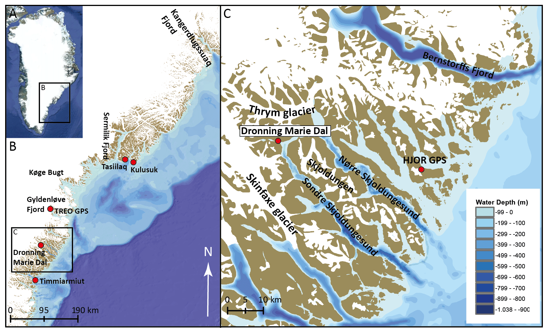
Figure 1 (a) Map of Greenland (©Google Earth). (b) The southeastern Greenland region, showing the location of the field site (Dronning Marie Dal) alongside other studied fjords. (c) Dronning Marie Dal salt marsh at the head of Sondre Skjoldungesund between the Skinfaxe and Thrum glacier margins.

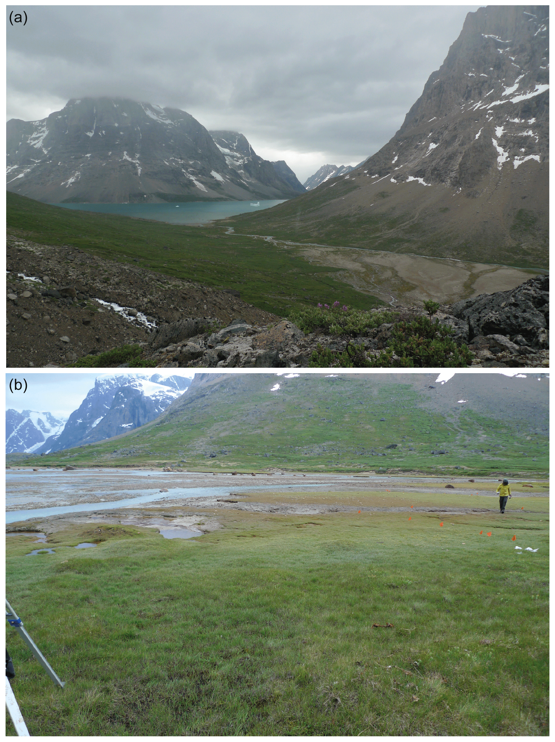
Figure 2 (a) Photograph looking east down the Dronning Marie Dal towards the head of Sondre Skoldungesund and the salt marsh where the valley meets the fjord. (b) Photograph of the Dronning Marie Dal salt marsh showing the low-angled relief of the marsh and zonation of salt marsh vegetation (high marsh in the foreground).

Relatively little is known about the deglacial history of southeastern Greenland compared to southwestern Greenland. Most work has been undertaken in the large fjords (e.g. Kangerdlugssuaq, Sermilik, Køge Bugt, Gyldenløve, Bernstorffs Fjord, Fig. 1) to the north of the field area using ¹⁰Be measurements to reconstruct fjord deglaciation. During the Last Glacial Maximum (LGM) the ice sheet reached the shelf edge (50–80 km from the outer coast) in this region, and in the offshore Kangerdlugssuaq Trough to the north of the study area the ice sheet started to retreat by ca. 17 ka BP (Funder et al., 2011). Onshore deglaciation at the outer coast occurred earlier to the north (Kangerdlugssuaq – 11.8±1 ka BP) compared to the south (Bernstorffs Fjord – 10.4±450 ka BP), driven by incursion of warm Atlantic water into the fjords from the Irminger Current, moderated by local coastal bathymetry and atmospheric warming during the early Holocene (Dyke et al., 2014, 2018; Hughes et al., 2012). The ¹⁰Be dates on boulders from outer and inner Skjoldungesund suggest deglaciation occurred here in the early Holocene (inner fjord by 10.4±0.4 ka BP) (Levy et al., 2020). Following retreat from the shelf edge, the deglaciation model HUY3 simulates retreat onshore by 10 ka BP, which largely agrees with the field evidence from Skjoldungesund, with the ice sheet slightly inland of its LIA maximum position at 4 ka BP (Lecavalier et al., 2014). The deglacial marine limit is low in this region (ca. 20–40 m), suggesting less deglacial mass loss compared to elsewhere in Greenland (Funder and Hansen, 1996). Observations of strandlines up to 75 m above sea level in this region, as reported by Vogt (1933), are cut into bedrock and are highly unlikely to be of marine origin.

The HUY3 geophysical model predicts slight crustal subsidence at the coast today caused primarily by a local Late Holocene neoglacial readvance (resulting in RSL rise of 1–1.5 mm yr⁻¹ over the last 1000 years) (Lecavalier et al., 2014). However, a recent GPS-derived GIA model (GNET-GIA) offers an alternative solution with GIA uplift calculated at +2.8 and +3.1 mm yr⁻¹ at nearby HJOR and TREO GPS sites (Fig. 1), which would result in pre-20th-century RSL fall at Dronning Marie Dal (Khan et al., 2016). By comparing GPS data and absolute gravity observations over a 20-year period, van Dam et al. (2017) also suggest ongoing GIA uplift of $+\mathrm{4.5}\pm \mathrm{1.4}$ mm yr⁻¹ at Kulusuk (300 km to the north). These GIA estimates, based on modern observations, are corrected for elastic deformation in response to modern mass balance changes to predict ongoing deglacial GIA. The most recent examination of Greenland GIA model outputs and GPS data by Adhikari et al. (2021) suggests that residual uplift caused by mass loss since the Medieval Warm Period, and in particular since the LIA, accompanied by a reduced mantle viscosity on sub-centennial timescales, can explain the observed discrepancy between uplift rates from HUY3 and elastic-corrected GPS uplift rates around Greenland.

LIA moraines are situated ahead of the current frontal margins of the GrIS and local glaciers in this region and demonstrate clearly that glacial retreat has occurred during the 20th century (Bjork et al., 2012). The instrumental temperature record from Tasiilaq indicates 2 ^∘C per decade of warming between 1919 and 1932 CE (the early 20th-century warming – ECW), followed by cooling during the 1950s to 1970s and a steady temperature rise of 1.3 ^∘C per decade since 1993 (Bjork et al., 2012; Chylek et al., 2006; Wood and Overland, 2010). Despite these decadal temperature fluctuations and the overall pattern of post-LIA retreat of southeastern Greenland glaciers, the nearest glaciers to the field site (Skinfaxe and Thrym, Fig. 1c) have been relatively stable at their present positions since at least the 1930s (Bjork et al., 2012). It is important to note, however, that Skinfaxe sits on a ledge in its fjord system, and thus it would require significant thinning to dislodge it from its current position, and Thrym Glacier appears to be resting on a shallow bedrock rise (Bjork et al., 2012; Morlighem et al., 2017). The total ice mass loss from the two drainage basins closest to the field site (“Central East” and “South-East” in Kjeldsen et al., 2015) is 249 Gt between the end of the LIA and 1983, 134 Gt between 1983 and 2003, and 45 Gt between 2003 and 2010 based on the volume of loss from LIA trimlines and more recent air photos. There is a significant increase (∼70 %) in the amount of regional mass loss during the post-1983 period compared to earlier in the 20th century. We hypothesise that regional ice mass loss since the end of the LIA should produce a viscoelastic GIA response that is recorded as variable 20th century RSL change by local salt marsh sediments, such as those at Dronning Marie Dal (Fig. 2).

2.2 Reconstructing RSL using salt marsh sediments

We collected salt marsh sediments by digging a small pit using a spade from the present-day high salt marsh at the mouth of Dronning Marie Dal (Figs. 1c and 2). The analysed sediment section is 13 cm thick, with organic silt containing saltwater-tolerant diatoms situated over compacted sand-rich silt where no diatoms are present (Fig. 3). We sampled the fossil sediment section at 0.25 cm intervals in the top 1 cm and at 0.5 cm intervals further downcore to provide high-resolution RSL estimates, bearing in mind the slow rate of sedimentation in most Greenlandic salt marshes (Long et al., 2012; Woodroffe and Long, 2009). To reconstruct local RSL we investigated diatom assemblages across the present-day salt marsh in the same location to understand changes in assemblages with elevation across the upper part of the intertidal zone (Fig. 3a). We then compared these assemblages to those found through the sediment core using a visual assessment technique that places weight on certain taxa that change abundance at clearly defined elevations (Long et al., 2010, 2012; Woodroffe and Long, 2009). The main species used to reconstruct RSL are the high marsh or freshwater species Pinnularia intermedia and the high to low marsh species Navicula cincta and Navicula salinarum. Using elevation zones inhabited by key species alone to reconstruct RSL introduces artificial jumps into a RSL record when moving from a sample reconstructed from within one zone to the next sample that may be reconstructed in a different zone. To create an RSL reconstruction with no artificial jumps within it we use a smoothing function that allows the PMSE (palaeo-marsh surface elevation) to change within each zone, noting the progressive way that the key diatom taxa change up the core. For instance the progressive rise in Pinnularia intermedia in the top 4 cm suggests smoothly falling RSL during this period. We therefore modify the PMSE results for the zoned reconstruction to allow for the progressive change seen in the diatoms (Table S2). This is backed up by the loss-on-ignition (LOI) data, which suggest a progressive rise in organic content in the top 4 cm indicative of rising PMSE. We prefer this method over a transfer function approach (e.g. Barlow et al., 2013) because it relies on certain indicator species that occur at narrowly defined levels but also utilises other evidence such as vertical diatom succession and the stratigraphy to interpret changes in RSL. In addition, we do not tune the RSL reconstructions to present-day RSL, rather the most recent index point reflects its diatom-based reconstruction, and therefore present-day RSL lies within the vertical error term of this reconstruction. This is done to prevent a spurious jump in recent RSL caused by a vertical offset between the mid-point in the earlier diatom-based reconstructions and the present-day marsh surface elevation, which would happen if this was used to tune the core top sample reconstruction.

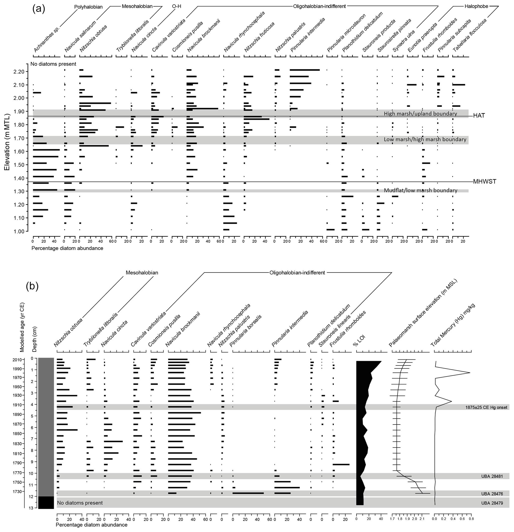
Figure 3 (a) Modern diatom data from the marsh at Dronning Marie Dal. Data are expressed as % total diatom valves (% TDV). Only data > 10 % TDV are shown. (b) Fossil diatom counts, palaeo-marsh surface elevation reconstruction and total mercury measurements from the Dronning Marie Dal salt marsh core. Diatoms are expressed as a % TDV, and only taxa with >10 % TDV are shown. Stratigraphy is shown in the left-hand box where grey indicates salt marsh sediment and black freshwater peat. Total mercury (mg kg⁻¹) was measured on salt marsh sediment using quadrapole inductively coupled plasma mass spectrometry (ICP-MS).

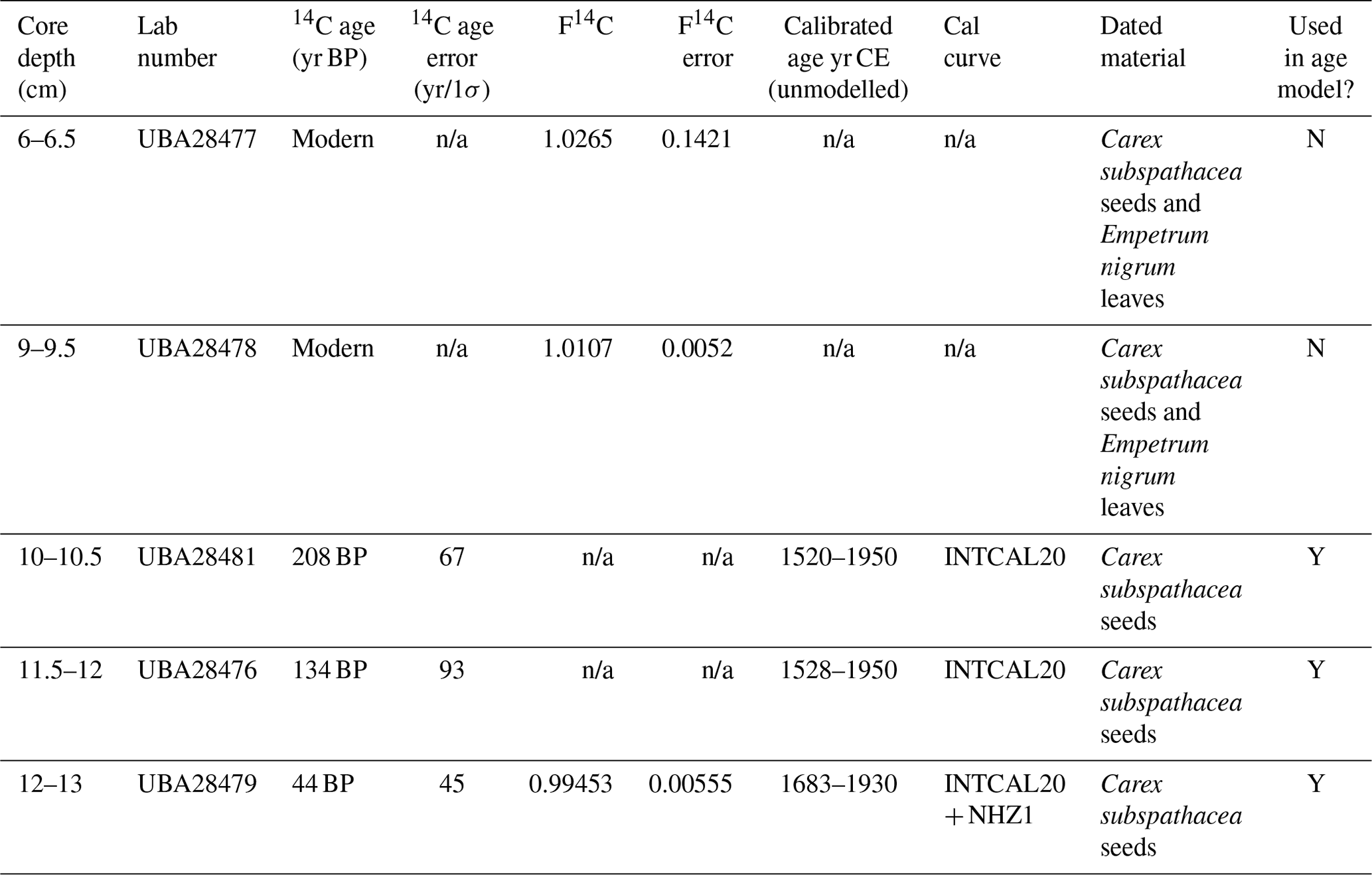
Table 1 Radiocarbon-dated samples from the Dronning Marie Dal salt marsh core. Samples at 6–6.5 and 9–9.5 cm are not included in the chronology because they were on extremely small samples (<0.3 mg when graphitised) and mix seeds and leaves from different sources. Note that n/a stands for not applicable.

We initially calculated the elevations of modern and fossil salt marsh samples to mean sea level (m.s.l.) using a high-precision differential global positioning system (DGPS). However, due to technical issues with post-processing, we instead rely on tidal data from Timmiarmiut (100 km to the south) and tidal predictions from Tasiilaq (300 km to the northeast) collected during our fieldwork, along with knowledge about salt marsh vegetation zonation in Greenland and their general relationship to tidal levels, to relate fossil and modern salt marsh elevations to mean sea level (m.s.l.). The tidal data from Timmiarmiut show that despite the timing of daily tidal fluctuations differing from predictions for Tasiilaq, the amplitude of tidal fluctuations is remarkably similar (within 0.1 m). The tidal range (lowest to highest astronomical tide) at the outer coast is approximately 3.7 m. We therefore have some confidence that tidal predictions for Tasiilaq are applicable (with a time correction) along the outer coast anywhere between Tasiilaq and Timmiarmiut despite the distances involved being large. This leaves the issue of tidal range amplification or dampening in fjord head settings to consider, as the Dronning Marie Dal site is ca. 50 km up the fjord from the open ocean (Fig. 1c). This is considered elsewhere in Greenland by Richter et al. (2011), who show that this effect is variable due to fjord bathymetry and cross section geometry and ranges from −9 to +14 cm up the fjord compared to the fjord mouths on the western coast in fjords of similar length to Søndre Skoldungesund. Modern salt marsh vegetation at Dronning Marie Dal grows between 0.1 m above the highest astronomical tide (HAT) and 0.08 m below the mean high water of spring tide (MHWST) levels, which is very similar to salt marsh vegetation ranges we have observed elsewhere in southeastern and southwestern Greenland (unpublished data and Woodroffe and Long, 2009, 2010). We are therefore confident that any effect of the fjord head setting on tidal range is small. We have not included an uncertainty estimate in our overall RSL reconstruction to reflect this because the uncertainty in the proxy elevations is already of a similar magnitude (±0.10–0.15 m; see Table A2).

2.3 Chronology

To provide a chronology to constrain the timing of reconstructed RSL changes, we use a range of complementary methods to maximise the precision of the resultant age–depth model. Very low concentrations of ²¹⁰Pb in the sediments required us to use other methods to provide recent sedimentation rates. We investigated the presence of total mercury (Hg) (mg kg⁻¹, which includes both mineral and atmospheric deposition) within the sediments using acid dissolution and quadrapole ICP-MS as an indicator of anthropogenic emissions. Other studies in western and northern Greenland note that between 1850 and 1900 CE there is more than a 2-fold increase in abundance of total Hg in lake sediments compared to Late Holocene levels (Bindler et al., 2001; Lindeberg et al., 2006; Shotyk et al., 2003; Zheng, 2015), whereas Perez-Rodriguez et al. (2018) see a rapid increase in Hg abundance from 1880 onwards in southern Greenland. We therefore assume that the onset of detectable Hg above background level in the Dronning Marie Dal salt marsh sediments at 4–4.5 cm indicates an age of 1850–1900 CE and use 1875±25 CE in the age–depth modelling described below. For the earlier part of the sediment record we submitted seeds and leaves from salt marsh and nearby freshwater plants picked from multiple horizons within the sediment for accelerator mass spectrometry (AMS) ¹⁴C dating at the ¹⁴Chrono centre at Queen's University, Belfast (Table 1). We generated an age–depth model for the whole sequence using the P_Sequence approach with variable k in Oxcal v. 4.3 using the IntCal20 calibration curve (Bronk Ramsey, 2009; Ramsey and Lee, 2013; Reimer et al., 2020). The resultant age–depth model uses the Hg chronohorizon (1850–1900 CE) and three ¹⁴C dates from lower in the sequence to estimate the age of every 0.25 cm of sediment in the sediment section with associated uncertainty (Tables A1 and A2). The chronological uncertainty reported throughout this study is the 95 % probability distribution (Bronk Ramsey, 2009).

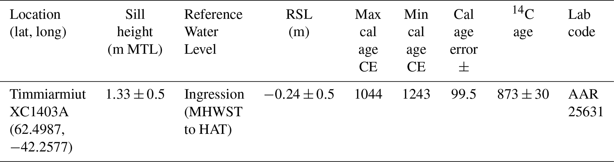
Table 2 Isolation basin sea level index point from Timmiarmiut used to calculate the rate of RSL due to ongoing GIA in this study.

We exclude the ¹⁴C ages at 6–6.5 cm (UBA28477) and 9–9.5 cm (UBA28478) from the age–depth model because they were on extremely small samples (<0.3 mg carbon) and are from samples that mix seeds and leaves from high salt marshes with freshwater plants that would not have been growing close together at the time (based on the palaeoenvironment recorded by the fossil diatom assemblage and the distribution of diatoms and vegetation types on the present-day salt marsh) (Table 1). The dated macrofossils from lower in the sequence are more likely to be autochthonous, as the diatoms record a high-marsh-to-freshwater environment this is close to HAT at the time of deposition.

2.4 Modelling RSL

2.4.1 Deglacial RSL change

There is a high degree of uncertainty in the rate of GIA in southeastern Greenland, owing largely to the lack of Holocene RSL data points to constrain deglacial history. Marine ingression into an isolation basin at Timmiarmiut (100 km SW of Dronning Marie Dal) at ca. 1140 CE (Table 2, also see Figs. A1, A2 and Table A1) gives an empirical estimate of regional GIA and suggests that the linear rate of background RSL change over the past millennium is in the range of +0.2 to +0.8 mm yr⁻¹ (Table 2). We therefore use a mid-point value of +0.5 mm yr⁻¹ as the rate of RSL change due to ongoing deglacial GIA in this study, rather than model predictions outlined in Sect. 2.1 which are not validated using RSL data from this region.

2.4.2 Post-LIA Greenland contribution

The post-LIA contribution to RSL at Dronning Marie Dal is computed using the sea level algorithm of Kendall et al. (2005) computerised by Mitrovica and Milne (2003). This code computes the geoidal and crustal response to ice and ocean loads on a spherically symmetric Earth discretised into 25 km thick elastic layers as defined by Dziewonski and Anderson (1981) and three viscous layers comprising a lithosphere, upper mantle and lower mantle. Lithospheric thicknesses (L) in the range 71–120 km are considered, with upper-mantle (ν_UM) and lower-mantle (ν_LM) viscosities of 0.1–1×10²¹ and 1–50×10²¹ Pa s explored to quantify the effect on predicted RSL change of different assumptions about Earth's viscosity structure. The post-LIA ice history for the GrIS is derived from Kjeldsen et al. (2015), who used a collection of aerial imagery from 1978–1987 CE to compare to historical trimlines assumed to be indicative of a maximum LIA position of the ice sheet; they also use 1900 CE as a Greenland-wide year of retreat from the maximum position and acknowledge considerable local and regional differences. The method for the extrapolation of point-scale changes in ice thickness over this time period to the rest of the Greenland Ice Sheet is detailed in the methods section of Kjeldsen et al. (2015).

2.4.3 Contribution from Greenland glaciers

Changes in ice thickness in peripheral Greenland glaciers is determined in exactly the same way as the post-LIA Greenland contribution. The peripheral Greenland glacier mass balance history is extracted from Marzeion et al. (2015) and considered separately from the global glacier dataset (Sect. 2.4.4) due to their proximity to the field site; the RSL response is computed as described in Sect. 2.4.2.

2.4.4 Contribution from global glaciers

We calculate the sea level contribution from global glaciers by first computing the global fingerprint for a +1 mm yr⁻¹ barystatic contribution from glacier complexes defined in Marzeion et al. (2012, 2015) since 1902. For the purposes of this calculation, we distribute the mass change across the glacierised regions equally since the use of a 512 harmonic truncation masks sub 100 km scale variability in ice thickness change across regions outside of Greenland. Ice thickness change will vary internally in each glacierised area, but the great distance between southeastern Greenland and many of the sources of melt means that the solution is insensitive to spatially inhomogeneous changes in ice thickness within the source regions. Ice thickness changes for each of the global glacier complexes are discretised into decadal loading intervals, and the global sea level response is computed using the density configuration in the Preliminary Reference Earth Model (PREM) (Dziewonski and Anderson, 1981). We use a lithospheric thickness of 96 km to represent a global average applied to all glacial sites and omit the viscous component from this calculation. Dronning Marie Dal is proximal to glacier sources in Iceland and Baffin Bay and thus should display some level of sensitivity to ice loss distribution over these glacierised areas. However, it is in the “near field” with respect to both of these sites, and therefore the use of a more realistic ice loss distribution in these areas (e.g. peripheral thinning) will reduce the relative sea level rise recorded in southeastern Greenland. The influence of low-latitude glaciers is excluded from the sea level fingerprint calculations, as the areas of mass loss are below the spatial resolution of the fingerprinting code. This simplified method produces similar results to that of Frederikse et al. (2020).

2.4.5 Contribution from the Antarctic Ice Sheet

Loss of ice mass from either the East Antarctic Ice Sheet or West Antarctic Ice Sheet will produce a relatively uniform sea level change fingerprint over the Northern Hemisphere (Bamber and Riva, 2010; Mitrovica et al., 2001). Recent Antarctic Ice Sheet change (1992–present) is relatively well documented and quantified (Meredith et al., 2019) compared to the period represented by the RSL data in this study. However, a recent study by Frederikse et al. (2020) that applied a Monte Carlo approach to balance the budget of global sea level rise since 1900 used estimates of 20th-century Antarctic Ice Sheet mass balance obtained from Adhikari et al. (2018) where the focus of mass loss throughout the 20th century is thought to be in the West Antarctic Ice Sheet, amounting to a global sea level change of 0.05±0.04 mm yr⁻¹. We use the resulting ensemble from the Frederikse et al. (2020) analysis to compute Antarctic Ice Sheet contribution at Dronning Marie Dal.

2.4.6 Contribution from steric changes

To compute the contribution from salinity and temperature changes in the nearby ocean, the Thermodynamic Equation of Sea Water (McDougall and Barker, 2011) (algorithm available here: https://www.teos-10.org/, last access: 1 October 2022) was applied to compute the steric height of the ocean. This uses a suite of proximal monthly temperature–depth and salinity–depth profiles extracted from the CMIP6 database for the “historical” experiments covering the period 1850–2014. The “historical” experiment was chosen to produce time series of depth-dependent potential temperature and salinity because the experiment forms part of the principal set of CMIP6 simulations, and the forcing datasets provided to the Atmosphere–Ocean General Circulation Models (AOGCMs) are consistent with a set of atmospheric and ocean observations (Eyring et al., 2016). We use only one configuration of the variant ID, which relates to initialisation time and procedure, specific model physics, and forcing (r1i1p1f1) across all AOGCMs considered (NASA-GISS-E2, CESM2, AWI, CanESM5 and FGOALS). The model output from the CMIP6 database has a spatial resolution in the range of 50–200 km, so we use profiles located within 300 km of Dronning Marie Dal to calculate an average trend in steric height for the nearby ocean. The steric heights are computed to reference depth levels of 500, 1000, 2000 and 3000 m. Computing steric heights to different reference levels allow us to determine which depth(s) in the ocean are contributing to steric height variability. Ivchenko et al. (2008) determined that for the North Atlantic for the period 1996–2006, applying a reference level of 1000–1500 m was sufficient to capture steric height variability, although this study provides trends in steric height across the maximum depth level available found in each model in the region proximal to Dronning Marie Dal.

2.4.7 Terrestrial water storage

To estimate the contribution of changes in terrestrial water storage we utilise the ensemble of time series of Frederikse et al. (2020) covering the time period 1900–2018 CE. This dataset was compiled by including the effects of natural variability in water reservoirs attributed to hemispheric-scale atmospheric and ocean circulation changes (Humphrey and Gudmundsson, 2019), changes in storage from dam building (Chao et al., 2008), and groundwater depletion activities (Döll et al., 2014; Wada et al., 2016).

In the next section the results from the field work, RSL reconstruction and sea level modelling are then compared to better understand changes in mass balance and RSL over recent centuries in southeastern Greenland.

3 Results

3.1 Modern diatom assemblages

Diatoms are zoned by elevation across the upper part of the intertidal zone at Dronning Marie Dal, with individual species providing useful information for reconstructing RSL. Above 2.2 m mean tide level (MTL) (>0.34 m above HAT) no diatoms were found in surface sediments, probably because the environment is too arid. There is a distinctive assemblage containing Pinnularia intermedia (>10 % at HAT, increasing to ∼55 % in the highest samples) that ends at ∼2.2 m MTL. We use this as a proxy sea level indicator to reconstruct palaeo-marsh surface elevation changes when we find Pinnularia intermedia to be either <10 %, between 10 % and 20 %, or above 20 % in fossil counts (Fig. 3a and b and Table A2). These zones are supplemented at lower elevations by a relatively narrow assemblage zone in the high to low marsh where Pinnularia intermedia values are negligible, Navicula cinta is >5 % and Navicula salinarum is not present (Fig. 3a and Table A2). We find these diatom assemblage zones in every marsh we have studied in southeastern and southwestern Greenland and use them to reconstruct RSL rather than using a transfer function approach as their precision is as good as or better (Pinnularia intermedia is present in >15 marshes between 59 and 69^∘ N in southwestern and southeastern Greenland with a vertical range of 0.2–0.4 m; unpublished data; Long et al., 2010, 2012; Woodroffe and Long, 2009, 2010). This approach also allows us to consider changes in other parameters (e.g. changes in these species abundance between samples and sediment Loss on Ignition) when producing palaeo-marsh surface elevation estimates.

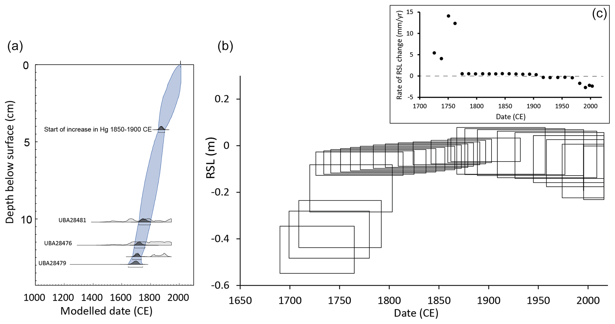
Figure 4 (a) Age–depth model using three ¹⁴C ages and the Hg chronohorizon. (b) Dronning Marie Dal RSL curve. (c) Rates of RSL change through time inferred from the RSL and age data.

3.2 Core stratigraphy and biostratigraphy

The core stratigraphy consists of a compacted basal freshwater organic silt-clay, grading upwards into organic high salt marsh sediments, and then into a slightly silt-rich organic low salt marsh towards the surface, with an increase in LOI values towards the surface (Fig. 3b). Diatoms are well preserved in the core and show a trend of falling palaeo-marsh surface elevation upwards from the base of the sequence as Pinnularia intermedia declines and Navicula cincta increases in abundance (alongside the absence of low marsh species Navicula salinarum, which provides additional information about palaeo-marsh surface elevations in this part of the core). In the top 3 cm Pinnularia intermedia increases in abundance with the recording showing RSL beginning to fall and palaeo-marsh surface elevation increasing (Fig. 3b).

3.3 RSL reconstructions

The salt marsh sediments and diatoms indicate long-term RSL rise. The rate of RSL rise at the start of the record ($+\sim \mathrm{7}$ mm yr⁻¹ between 1725 and 1762 CE; Fig. 4b and c) is significantly higher than the rate reconstructed from the closest isolation basin at Timmiarmiut ($+\mathrm{0.5}\pm \mathrm{0.3}$ mm yr⁻¹; Table 2). This may be due to LIA ice growth, including the nearby Skinfaxe glacier delivering sediment-laden meltwater to Dronning Marie Dal, causing local ice loading and rapid infilling of accommodation space and salt marsh development. The rate of RSL rise declines rapidly over the period 1762–1880 CE to +0.4 mm yr⁻¹ and is within the error range of the isolation basin rate during most of this period ($+\mathrm{0.5}\pm \mathrm{0.3}$ mm yr⁻¹). This trend of rapid and then slowly rising RSL between 1725 and 1880 CE is likely due to changes in the local LIA ice load over this time period combined with ongoing millennial-scale GIA. The HUY3 model predicts +1.44 mm yr⁻¹ of RSL rise over the past 1000 years in this region (Lecavalier et al., 2014), which is larger than (but the same sign as) the salt marsh and isolation basin RSL data during this period. Other recent estimates of centennial-scale GIA (Khan et al., 2016; van Dam et al., 2017) suggest that RSL should have been falling over the past few hundred years at Dronning Marie Dal. The isolation basin and salt marsh data instead suggest that RSL was rising or close to stable from ca. 1100 CE until ca. 1880 CE.

From 1880 CE RSL began to fall, which is indicated clearly in the diatom record by the decline in Navicula cincta up the core and the reintroduction and increasing abundance of Pinnularia intermedia, a high marsh diatom species, after 1900 CE (Fig. 3b). There is $\sim \mathrm{0.09}\pm \mathrm{0.1}$ m of RSL fall since 1880 CE, which if calculated as a constant rate of change is $-\mathrm{0.72}\pm \mathrm{1.7}$ mm yr⁻¹ RSL fall (Fig. 4b and c, Tables 3 and A2). Because of the lack of direct dating control in upper part of the core and the slow rate of sedimentation it is not possible to infer decadal changes in RSL rate during the 20th century.

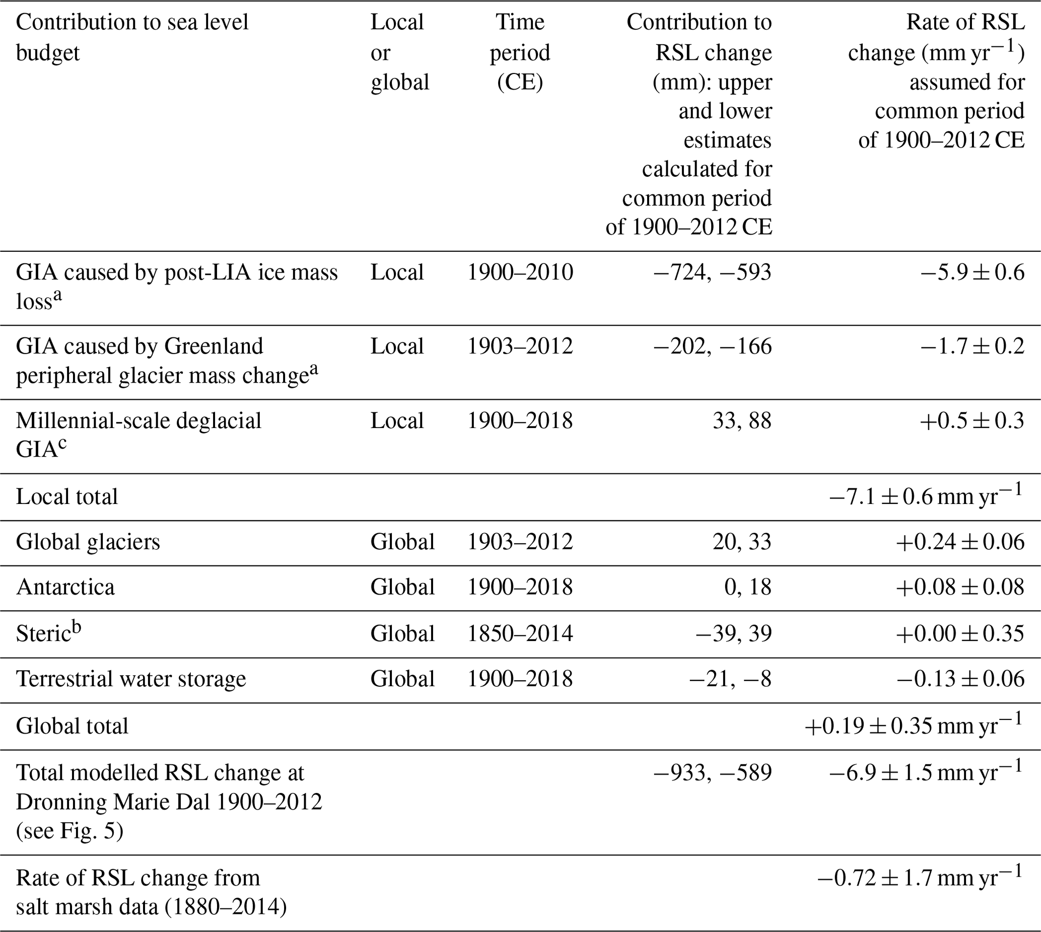
Table 3 Calculated amounts and rates of RSL change from the various contributors to the RSL budget at Dronning Marie Dal. Rates of RSL change are supplied with ±2σ uncertainty unless specified: a uncertainty reflects assumed ±10 % error on rates that are larger than ±2σ. ^b Steric sea level contribution calculated from the average of significant trends for the 0–2000 m depth interval from three models in Table 4. ^c GIA from nearby isolation basin ingression with uncertainty calculated from upper- and lower-elevation reconstruction uncertainties.

3.4 Modelled RSL changes

Published calculations of post-LIA Greenland mass loss and other RSL contributors start at 1900 CE (e.g. Kjeldsen et al., 2015; Marzeion et al., 2015), so we focus on this part of the salt marsh RSL record to compare the reconstructed RSL with a modelled sea level budget. The different contributions to the sea level budget are summarised in Table 3 and Fig. 5. For an average Earth model configuration of L=96 km, ${\mathit{\nu }}_{\mathrm{UM}}=\mathrm{0.5}\times {\mathrm{10}}^{\mathrm{21}}$ Pa s and ${\mathit{\nu }}_{\mathrm{LM}}=\mathrm{10}\times {\mathrm{10}}^{\mathrm{21}}$ Pa s, post-LIA ice mass loss (from the GrIS only) resulted in sea level change of −5.9 mm yr⁻¹ at Dronning Marie Dal between 1900 and 2010 CE. Between 1983 and 2010 CE the modelled RSL rate was −10.1 mm yr⁻¹. Any chosen Earth configuration within the parameter range explored does not significantly affect the predicted sea level change; for 1900–2010 CE, the range of RSL fall was between −6.7 and −5.8 mm yr⁻¹, and for 1983–2010 CE it was between −11.7 and −9.9 mm yr⁻¹. Using a fixed lithospheric thickness of 96 km, the modelled total sea level fall arising from post-LIA mass loss across a suite of Earth models with upper-mantle viscosities ranging from 5×10¹⁹ to 1×10²² Pa s and lower-mantle viscosities in the range of 1×10²¹–5x×10²² Pa s was 0.65 to 0.86 m, a difference of 0.21 m, which is within the uncertainty range of the RSL reconstruction (Fig. 4b). The upper-mantle viscosity is the largest contribution to this uncertainty, accounting for both upper and lower bounds of this range. The effect of reducing the lithospheric thickness from 120 to 46 km reduces the amount of modelled relative sea level fall by only a few centimetres. The contribution of peripheral Greenland glaciers to RSL was on average $-\mathrm{1.7}\pm \mathrm{0.2}$ mm yr⁻¹ between 1903 CE and present day; with decadal-scale contributions of −3 to −5 mm yr⁻¹ between 1923 and 1943 CE. Global glacier mass loss contributes $+\mathrm{0.24}\pm \mathrm{0.06}$ mm yr⁻¹ RSL rise between 1903 and 2009 CE. Antarctica has contributed more significantly to sea level change in recent years; for the period 1992 to 2016 CE, the Antarctic Peninsula and the West Antarctic Ice Sheet are thought to have resulted in $+\mathrm{0.06}\pm \mathrm{0.73}$ mm yr⁻¹ of barystatic sea level change (Meredith et al., 2019). However, for the period 1850–2014 CE Frederikse et al. (2020) compute $+\mathrm{0.08}\pm \mathrm{0.02}$ mm yr⁻¹, rising to +0.2 mm yr⁻¹ ± 0.05 mm yr⁻¹ between 1970 and 2018 CE.

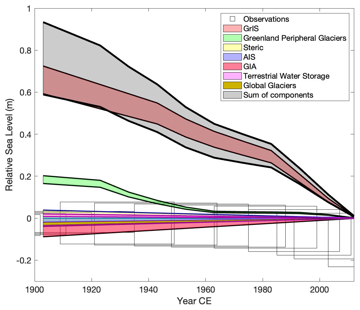
Figure 5 Observed and modelled relative sea level change from 1900 to 2010 CE as a function of recent and Late Holocene Greenland ice thickness changes (GIA caused by the GrIS, Greenland peripheral glaciers and millennial-scale GIA; the “local” signal) and from sources outside of Greenland (steric signal, the Antarctic Ice Sheet (AIS), terrestrial water storage and global glaciers). The sum of the modelled components is shown as the shaded grey area, and the GrIS and peripheral glacier contributions are shown with an estimated ±10 % uncertainty. The black crosses are the salt-marsh-based RSL reconstruction.

Table 4 Mean trends in steric height anomalies for three reference levels (500, 1000 and 2000 m) calculated from profiles within 300 km of Dronning Marie Dal using five models participating in the CMIP6 analysis. In all cases, the experiment variant ID was r1i1p1f1. Numbers in brackets denote number of profiles displaying significant trends in steric height from which the mean and 2σ trends were calculated. The AWI model produced no significant trends for either time period, while GISS-E2 did not produce significant trends for 1850–2014 CE.

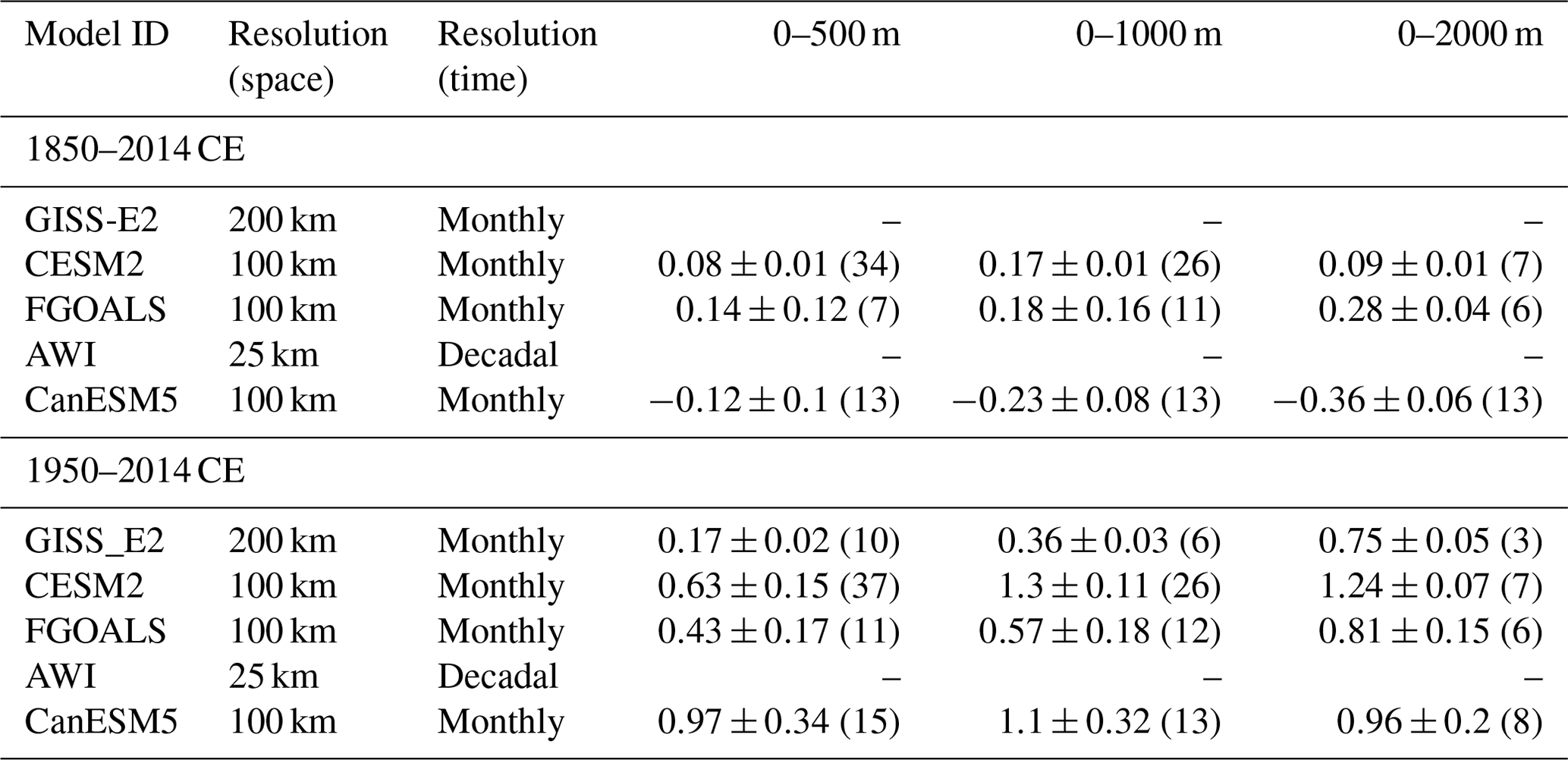
The range of values for the modelled steric contribution are in Table 4. They represent an upper estimate of the magnitude and range of the steric component as only profiles showing significant RSL trends are used when calculating the mean. From 1850 to 2014 CE, trends in steric height are in the range −0.23 to +0.18 mm yr⁻¹ for a reference depth level of 1000 m and −0.36 to +0.28 mm yr⁻¹ over a depth range of 2000 m. An observation-based analysis of trends in steric height by Frederikse et al. (2020) shows the steric contribution from the upper 2000 m of the ocean close to Dronning Marie Dal between 1957 and 2018 CE is +0.13 mm yr⁻¹ (we include steric trends derived for the period 1950–2014 in Table 4 for comparison). All models considered in Table 4 have larger values than the estimates of Frederikse et al. (2020). Finally, the impact of terrestrial water storage amounts to a sea level fall of $-\mathrm{0.13}\pm \mathrm{0.06}$ mm yr⁻¹ at Dronning Marie Dal over the 20th century.

The different contributions to RSL are summed and plotted alongside the salt marsh RSL data in Fig. 5. The sum of components predicts RSL fall of between 0.58 and 0.93 m since 1900 CE. This prediction is dominated by the contribution of GIA caused by post-LIA Greenland and peripheral glacier mass loss, which is only counteracted a little by the other components which mostly predict small amounts of RSL rise. The salt marsh data only reconstruct $\sim \mathrm{0.08}\pm \mathrm{0.1}$ m of RSL fall since 1880 CE, producing a large mismatch between the sea level budget and the salt marsh RSL data.

4 Discussion

The dominant contributors to post-LIA RSL change at Dronning Marie Dal are the adjustment of the solid Earth and changes in geoid height in response to both post-LIA and millennial-scale Greenland Ice Sheet changes. These contributors (ongoing GIA from the last deglaciation, post-LIA Greenland mass balance and mass loss from peripheral Greenland glaciers) amount to a modelled sea level fall of −7.1 mm yr⁻¹ between 1900 and 2010 CE. By contrast, the RSL contributors unrelated to cryospheric change in Greenland only amount to modelled sea level rise of +0.19 mm yr⁻¹, giving a total RSL fall of −6.9 mm yr⁻¹ between the end of the LIA and present (Table 3). This clearly does not fit with the observations from the salt marsh data (Figs. 4b and 5), which suggests that the rate of RSL fall between 1900 and 2013 CE is $-\mathrm{0.72}\pm \mathrm{1.7}$ mm yr⁻¹.

4.1 Timing of the end of the LIA and Greenland Ice Sheet and peripheral glacier contribution

To try to bring the post-LIA sea level budget closer to the salt marsh observations, we explore two possible sources of uncertainty in the dominant post-LIA Greenland signal: (1) timing of the start of post-LIA mass loss in Greenland and (2) greater uncertainty in modelled sea level associated with post-LIA GrIS and peripheral glacier mass loss.

To explore the possibility that the total post-LIA Greenland mass loss occurred over a longer time period, we create five scenarios where the LIA maximum ice termination in Greenland is adjusted to begin at 1700, 1750, 1800, 1850 and 1900 CE, and the rate of mass loss is scaled accordingly, with the end point remaining at 2010 (as in Kjeldsen et al., 2015). We know that the LIA ice sheet response was different around Greenland with multiple advance phases forced by different driving mechanisms, and it is simplistic to suggest that the whole of the ice sheet began to lose mass simultaneously at 1900 CE (Kjær et al., 2022), although it may serve as a Greenland-wide year. By adjusting the LIA termination date (and therefore the start of Greenland and peripheral glacier mass loss) we can investigate the impact of earlier ice retreat on RSL at Dronning Marie Dal. In this sensitivity analysis we recognise that moving the LIA termination date in our modelling means that we are assuming the LIA simultaneously ended earlier around the whole of Greenland, which is no more nuanced than assuming LIA termination at 1900 CE. We also note that the glaciers closest to Dronning Marie Dal appear to have been at their LIA maximum position in the early 20th century, which does not agree with an earlier LIA end in this location (Bjork et al., 2012), and a recent alkenone-based sea surface temperature reconstruction from Nørre Skjoldungesund suggests considerable warming here occurred later, between ca. 1915 and 1945 CE (Wangner et al., 2020). The analysis does, however, allow a first-order investigation into the sensitivity of modelled post-LIA sea level to the length of time over which the post-LIA mass loss occurred.

The second parameter that we vary as part of this sensitivity study is the total amount of post-LIA RSL change from the GrIS and peripheral glaciers, by assuming an error of up to −30 % on these calculations. Kjeldsen et al. (2015) report uncertainties in their mass loss estimates for the southeastern sector of the ice sheet between 7 % and 15 %, and so this sensitivity analysis allows us to test the effect on RSL at Dronning Marie Dal of a smaller amount of mass loss since the end of the LIA in this region.

Varying both LIA termination date and total post-LIA mass loss from the GrIS and peripheral glaciers affects how much sea level change from other components is required to close the post-LIA budget (Fig. 6). The “budget residual” in Fig. 6 refers to the misfit in millimetres per year between the RSL change reconstructed by the salt marsh data and RSL change predicted by the sea level budget calculations. In essence this is the amount of sea level change that we still need to “find” to close the budget even after we modify the timing and total amount of mass loss from the dominant contributors to RSL change in GrIS and peripheral glacier retreat since the end of the LIA.

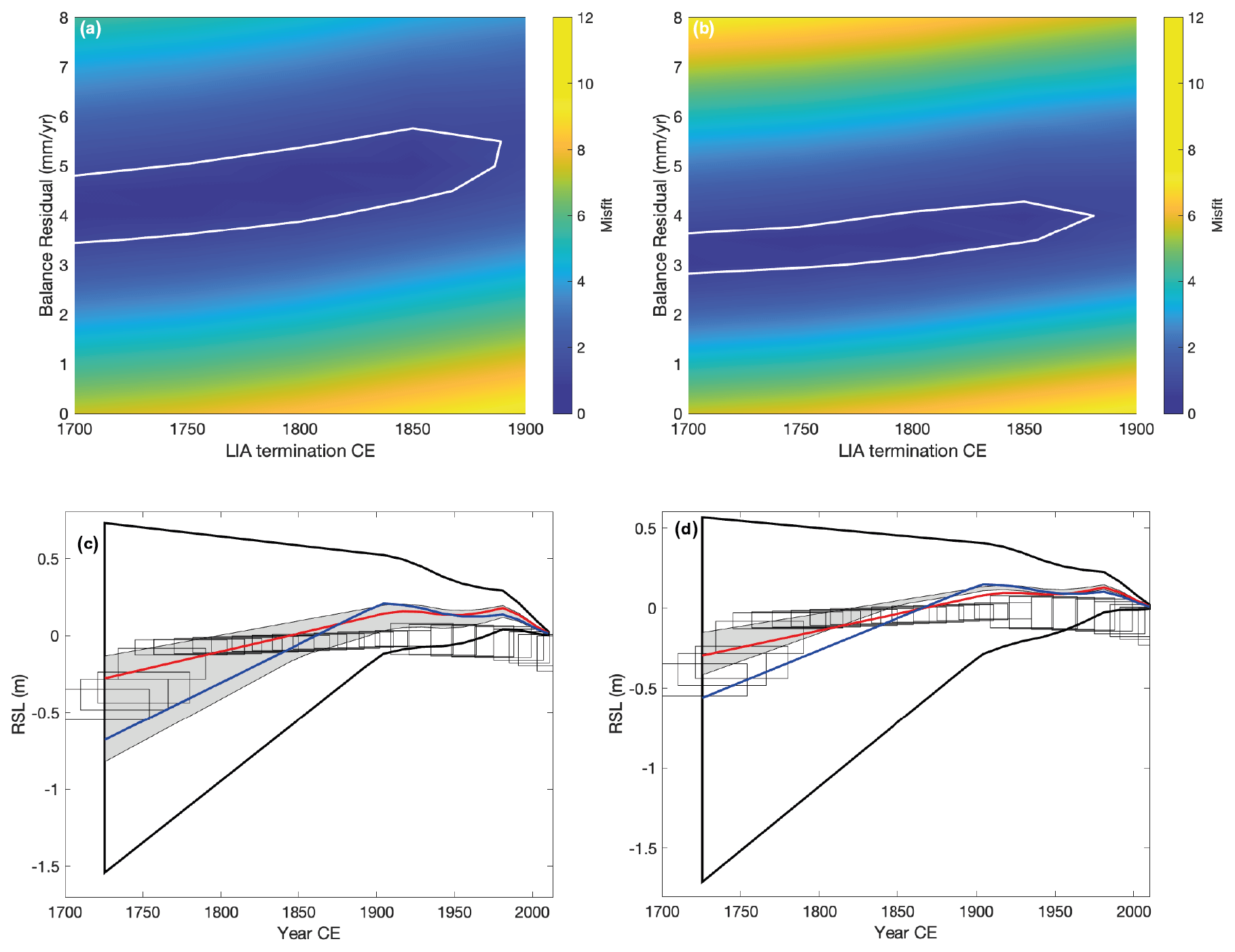
Figure 6 (a, b) Misfit plots showing model data fit where combinations of budget residuals and LIA termination dates are considered with (a) no assumed error in the RSL contribution from the GrIS and (b) a 30 % reduction in magnitude of sea level change associated with local changes in the GrIS. Areas within the white lines have a statistically equivalent fit to the RSL data. (c) Modelled RSL from all combinations of LIA termination date and budget residual, assuming no error in the RSL contribution from the GrIS. Area within the black line denotes all possible combinations of RSL trends from LIA terminations from 1750 to 1900 CE and budget residual rates between 0 and 6 mm yr⁻¹. The shaded grey area corresponds to RSL trends from within white lines in (a), demonstrating a statistically equivalent fit to the data. For illustrative purposes, the red line denotes a modelled RSL scenario with a LIA termination date of 1900 CE (assumed LIA termination date in Kjeldsen et al., 2015) and a budget residual rate of +4 mm yr⁻¹, while the blue line shows a modelled RSL scenario with a budget residual rate of +5 mm yr⁻¹ and LIA termination date of 1900 CE. Panel (d) is the same as panel (c) except the shaded grey area corresponds to RSL trends from (b), demonstrating a statistically equivalent fit to the data. For illustrative purposes, the red line denotes a modelled RSL scenario with a budget residual rate of +3 mm yr⁻¹ and LIA termination date of 1700 CE, while the blue line shows a modelled RSL scenario with a budget residual rate of +4 mm yr⁻¹ and LIA termination date of 1700 CE.

The time period over which post-LIA mass loss occurs is important for understanding the degree of volume mismatch between the RSL observations and modelled contributions from the maximum extent to present. Figure 6a indicates that moving the LIA termination date from 1900 to 1700 CE reduces the budget residual required to fit the RSL data from $\sim +\mathrm{5}$ to $\sim +\mathrm{4}$ mm yr⁻¹. This residual is reduced further (to $\sim +\mathrm{3}$ mm yr⁻¹) when considered alongside a 30 % reduction in the amount of RSL fall originating from the GrIS and peripheral glaciers compared to values computed using RSL from ice histories generated by Kjeldsen et al. (2015) (GrIS) and Marzeion et al. (2015) (peripheral glaciers) (Fig. 6b). Figure 6c and d further illustrate these results. Figure 6c, where there is no reduction in the amount of post-LIA mass loss, shows a poor fit to the RSL data when the LIA termination is moved to between 1700 and 1800 CE, and there remains a +3.5 to 5 mm yr⁻¹ budget residual that must be accounted for from other parts of the sea level budget. In Fig. 6d, a better fit to the RSL data is possible with a 30 % reduction in Greenland and peripheral glacier mass loss and LIA termination at 1800 CE. The remaining budget residual is +3 mm yr⁻¹, which again must be accounted for from other parts of the sea level budget.

The smallest calculated budget residual ($\sim +\mathrm{3}$ mm yr⁻¹) has to be found from processes causing sea level rise in southeastern Greenland, such as millennial-scale Greenland GIA, Antarctic Ice Sheet melt, the steric effect and global glacier melt. The modelled sea level budget suggests that these processes are only small contributors to total sea level change, with the sum of sources from outside Greenland only +0.19 mm yr⁻¹ since 1900 CE. The steric effect has the largest uncertainty, which we consider in Sect. 4.8 alongside other potential sources of error in our calculations. It is difficult, however, to see how the contributors to RSL rise in southeastern Greenland could be significantly larger before 1900 CE given the cooler regional temperatures of the LIA.

4.2 Reliability of salt marsh RSL data

Salt marshes and their microfossil communities are widely used in temperate locations and previously in western and southern Greenland to reconstruct recent RSL changes with high precision (e.g. Kemp et al., 2009, 2017; Long et al., 2010, 2012; Woodroffe and Long, 2009). At Dronning Marie Dal, the first half of the RSL record (1725–1880 CE) is harder to interpret because early and rapid RSL rise may indicate either a local LIA loading signal or a non-RSL factor (e.g. sediment supply changes) as the marsh became established. What we can say with certainty is that RSL began to fall at or soon after 1880 CE, suggesting additional contributors to RSL or changes in the dominance of existing contributors caused this change in the sign and rate of RSL. We are also confident in our assessment of the total amount of RSL fall between 1880 CE and present, which is less than predicted by any permutation of the sea level budget modelling (Fig. 5). We acknowledge, however, that these reconstructions come from a single sediment core. Although the stratigraphy appeared consistent across the marsh during fieldwork, it would be ideal to replicate these results within another core from the same marsh and also from other marshes close to the ice sheet margin in this region in the future.

There is no indication of hiatuses within the marsh sediment, and based on surveys of modern marshes here and elsewhere in Greenland the elevation range of the key diatom species Pinnularia intermedia used in the palaeo-marsh surface elevation calculations is robust. A RSL fall of ∼0.6–0.9 m since 1900 CE as predicted by the sea level budget modelling would have lifted what was a high marsh environment at the start of the period (indicated by the taxa at ∼5 cm depth, Fig. 3b) out of the intertidal and into the adjacent freshwater zone where diatoms are not preserved due to extreme aridity. The continuous preservation of intertidal diatoms through the sediment sequence to the surface where modern salt marsh plants were growing during sampling (Fig. 2) rules out this possibility. Even the smaller amount of RSL fall (∼0.2 m) since 1900 CE predicted by an earlier LIA termination date (1800 CE) and 30 % smaller GrIS contribution (Fig. 6) is unlikely because the diatoms suggest a mid-to-high marsh environment at 1900 CE and the core top elevation is within the high marsh zone, a vertical distance based on analysis of modern diatoms at Dronning Marie Dal of ∼0.1 m, which is half of the predicted RSL fall (∼0.2 m). Greenland salt marshes accrete very slowly and only record sustained RSL changes over decades, and therefore short-timescale variability in contributors (e.g. due to decadal temperature fluctuations in the 20th century) is not distinguishable in the salt marsh data. However, the total amount of RSL fall and the timing of the change from RSL rise and stability to RSL fall is robustly reconstructed, and we are confident that this provides an important test of Greenland RSL modelling.

4.3 Limitations of RSL modelling

Regional sea level budgets deviate significantly from the global budget, are challenging to compute, and have been deemed part of the “Regional Sea-Level Change and Coastal Impacts” Grand Challenge by the World Climate Research Programme (WCRP, 2015). Of the different items in the sea level budget for Dronning Marie Dal, the large uncertainty in the steric contribution could potentially be the source of additional sea level rise, which would help decrease the budget residual identified in Fig. 6. The data in Table 4 do not fully capture the range of uncertainty in the steric component of sea level. These uncertainties arise from poor to non-existent capture of the dynamics of coastal regions, namely the propagation of the change in steric height of the open ocean to the fjord location and the lack of observations required to constrain model output in the early 20th century.

The field site is located at the head of the 50 km long marine fjord Søndre Skoldungesund, and therefore the steric contribution may be different to that calculated from the open-ocean estimates within 300 km of Dronning Marie Dal averaged in this study. A multibeam study of the fjord by Kjeldsen et al. (2017) shows the fjord is between 1.1 and 3.1 km wide and up to 800 m deep in the outer part, with a shallow (77 m deep) sill mid-fjord and shallow depths inside the sill. The fjord water is cold to the base along its length, with no apparent intrusion of warmer Atlantic water from the shelf edge. The mixed predictions of steric height changes from the different models suggest that this region is poorly constrained within global steric datasets (Table 4). Given the lack of intrusion of warm Atlantic water into the fjord today it is unlikely that there has been a more positive contribution of steric height from 20th-century warming. However, with significant mass loss from the Greenland Ice Sheet since the LIA and an influx of cold yet low-salinity meltwater into the fjord it is possible that the local halosteric component is underestimated.

A second issue with the steric height calculation is the potential for the CMIP6 models to misrepresent changes in the dynamic height of the ocean caused by shifts in the location of ocean currents, such as the East Greenland Current (EGC), over time. A recent study of North Atlantic dynamic sea level and its response to GrIS meltwater and temperature increase indicates general Atlantic meridional overturning circulation decline and an increase in sea surface height with increased GrIS melting, but the response of the cold EGC is complex, and in southeastern Greenland the effect of warming and increased meltwater on sea surface height is minimal (Saenko et al., 2017). Given that Kjeldsen et al. (2017) suggest the EGC does not currently penetrate into the Søndre Skoldungesund fjord, the impact of any dynamical changes in the EGC since the LIA are likely to be minor.

A third possible source of uncertainty in the sea level budget is the application of the sea level code used to calculate GIA, specifically the spectral resolution with which the algorithm predicts the sea level response to loading increments. The mass balance history from Kjeldsen et al. (2015) is presented on a 1×1 km spatial grid, but the sea level code utilises a spectral harmonic truncation of 256. The effects on predicted RSL of the reduction in resolution have been demonstrated previously with near-field relative sea level being more affected by harmonic truncation than far-field sites (Spada and Melini, 2019). A move towards a higher degree of spherical harmonic truncation (>1024) would be necessary to faithfully reproduce sea level fingerprint histories associated with small outlet glaciers and should be considered in the future (Adhikari et al., 2016).

Despite the limitations outlined above, this study presents a first test of a post-LIA sea level budget in the near-field location of southeastern Greenland. There is a clear and unexplained difference between the RSL history recorded by salt marsh sediments (a small RSL fall since the end of the LIA) and the RSL budget, which suggests significant RSL fall during this period. The sensitivity tests show that the budget can fit the salt marsh RSL data if the amount of mass loss from the GrIS and peripheral glaciers is less and it took place over a longer period (Fig. 6d), but despite this a +3 mm yr⁻¹ unexplained budget residual remains. RSL reconstructions from salt marshes in southwestern Greenland (Long et al., 2010, 2012; Woodroffe and Long, 2009, 2010) also suggest that the dominant signal in southern Greenland is RSL rise into the 20th century, which correlates with the long-term (pre ∼ 1880 CE) trend of RSL rise at Dronning Marie Dal.

5 Conclusions

Salt marsh sediments collected at the mouth of Dronning Marie Dal, close to the GrIS margin in southeastern Greenland, record RSL changes over the past ca. 300 years in changing sediment and diatom stratigraphy. These RSL changes record a combination of processes that are dominated by local and regional changes in GrIS mass balance during this critical period that spans the maximum of the LIA and 20th-century warming.

In the early part of the record (1725–1762 CE) the rate of RSL rise is higher than reconstructed from the closest isolation basin at Timmiarmiut, but between 1762–1880 CE the rate decreases to within the error range of the isolation basin RSL rate. This trend is likely due to changes in the local LIA ice load over this time period combined with ongoing millennial-scale GIA or other local processes as the salt marsh is established. Other recent estimates of centennial-scale GIA (Khan et al., 2016; van Dam et al., 2017) suggest that RSL should have been falling over the past few hundred years at Dronning Marie Dal. The isolation basin and salt marsh data instead suggest that RSL was rising or close to stable from ca. 1100 CE until ca. 1880 CE. RSL begins to slowly fall around 1880 CE, with a total amount of RSL fall of 0.09±0.1 m since 1880 CE.

Modelled RSL, which takes into account contributions from post-LIA GrIS GIA, ongoing deglacial GIA, the global non-ice sheet glacial fingerprint, the contribution from thermosteric effects, an estimate of the Antarctic fingerprint and the contribution from terrestrial water storage, overpredicts the amount of RSL fall since the end of the LIA by at least 0.5 m. The GIA signal caused by post-LIA GrIS mass loss is by far the largest contributor, and error in its calculation has the largest potential to impact RSL predictions at Dronning Marie Dal. We cannot reconcile the modelled contributions and the salt marsh observations, even when moving the termination of the LIA to 1700 CE and reducing the post-LIA Greenland mass loss signal by 30 %. A budget residual of $\sim +\mathrm{3}$ mm yr⁻¹ since the end of the LIA remains unexplained. Explaining the difference between salt marsh RSL data and the modelled RSL budget since the end of the LIA and determining the timing of the LIA termination should be key future research objectives and can be addressed through reducing uncertainty in each component to the sea level budget, collecting more empirical data on the recent history of the GrIS, and by replicating the salt marsh RSL record presented here elsewhere in this and other regions of Greenland.

Appendix A

Table A1 Details of dating and RSL calculation for the ingression of basin XC1403A at Timmiarmiut, southeastern Greenland.

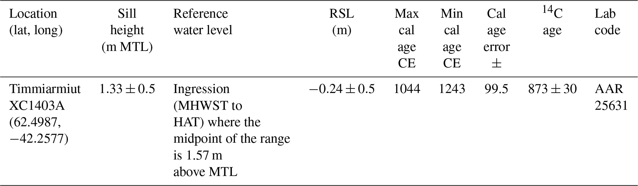
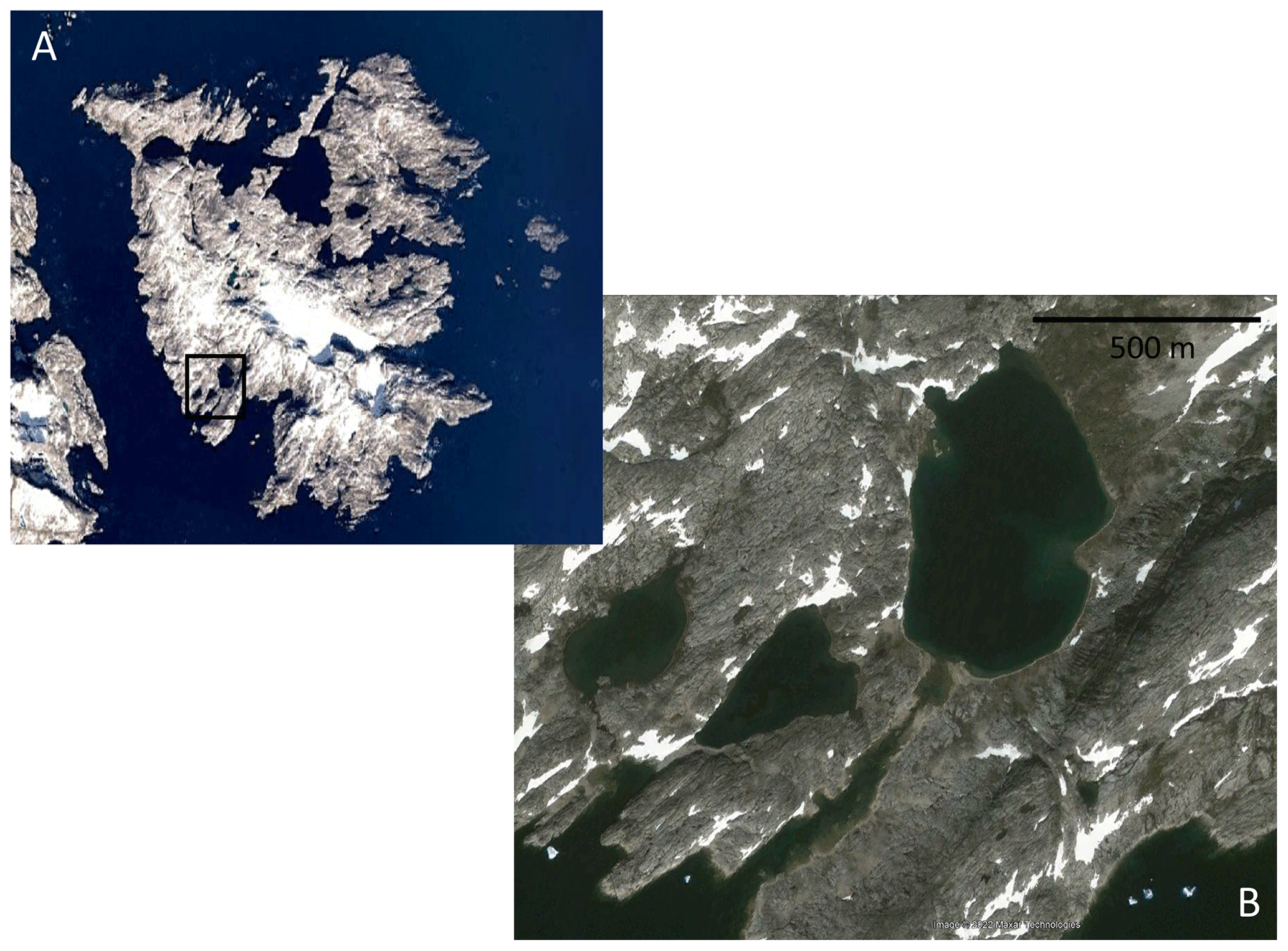
Figure A1 (a) Location of isolation basin (62.4987^∘ N, −42.2577^∘ W) on the island of Timmiarmiut (62.51^∘ N, −42.22^∘ W) in southeastern Greenland (source: “Timmiarmiut.” 62.515669, −42.206218. Google Earth © Landsat/Copernicus imagery, https://earth.google.com/web/, last access: 23 November 2022). (b) The basin is ∼450 m from west to east and ∼675 m from north to south at its largest point. The basin sill is 1.33±0.5 m a.m.s.l. (Source: “Lake XC1403.” 62.497715, −42.257307. Google Earth © Maxar Technologies image taken on 11 August 2009, https://earth.google.com/web/, last access: 23 November 2022).

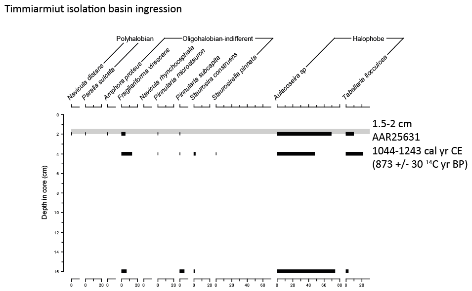
Figure A2 Fossil diatom counts from the top 16 cm of a core taken from isolation basin XC1403A showing the first occurrence of polyhalobian diatoms at 2–2.5 cm depth and assumed ingression of the basin at this point. The ¹⁴C sample is taken from 1.5–2 cm depth and represents tidal level between MHWST and HAT. The basin is surrounded by salt marsh vegetation at present day, indicating its elevation within the modern intertidal zone.

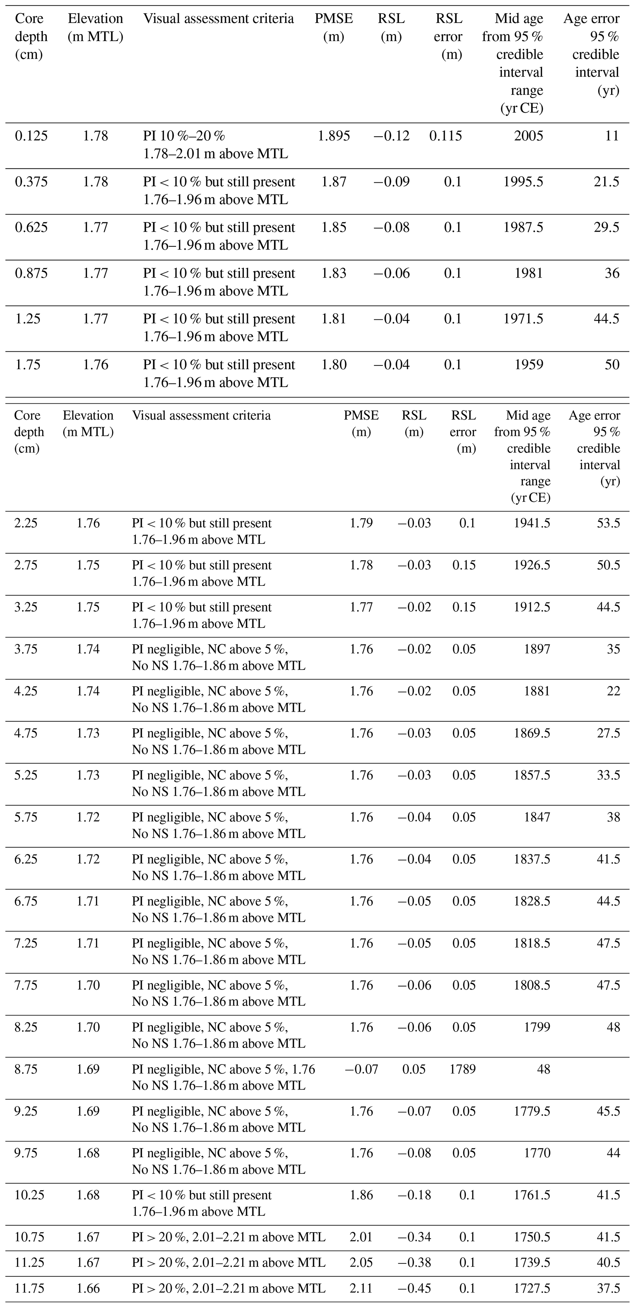
Table A2 Details of RSL calculations from salt marsh core at Dronning Marie Dal. Visual assessment criteria are as follows: PI is Pinnularia intermedia, NC is Navicula cincta, NS is Navicula salinarum. PMSE is palaeomarsh surface elevation. Tidal levels are calculated in relation to tidal levels at Tasiilaq (see Sect. 2.2 for information on tidal measurements).