Did the Bronze Age deforestation of Europe affect its climate? A regional climate model study using pollen-based land cover reconstructions

This paper studies the impact of land use and land cover change (LULCC) on the climate around 2500 years ago (2.5 ka), a period of rapid transitions across the European landscape. One global climate model was used to force two regional climate models (RCMs). The RCMs used two land cover descriptions. The first was from a dynamical vegetation model representing potential land cover, and the second was from a land cover description reconstructed from pollen data by statistical interpolation. The two different land covers enable us to study the impact of land cover on climate conditions. Since the difference in landscape openness between potential and reconstructed land cover is mostly due to LULCC, this can be taken as a measure of early anthropogenic effects on climate. Since the sensitivity to LULCC is dependent on the choice of climate model, we also use two RCMs.

The results show that the simulated 2.5 ka climate was warmer than the simulated pre-industrial (PI, 1850 CE) climate. The largest differences are seen in northern Europe, where the 2.5 ka climate is 2–4 ^∘C warmer than the PI period. In summer, the difference between the simulated 2.5 ka and PI climates is smaller (0–3 ^∘C), with the smallest differences in southern Europe. Differences in seasonal precipitation are mostly within ±10 %. In parts of northern Europe, the 2.5 ka climate is up to 30 % wetter in winter than that of the PI climate. In summer there is a tendency for the 2.5 ka climate to be drier than the PI climate in the Mediterranean region.

The results also suggest that LULCC at 2.5 ka impacted the climate in parts of Europe. Simulations including reconstructed LULCC (i.e. those using pollen-derived land cover descriptions) give up to 1 ^∘C higher temperature in parts of northern Europe in winter and up to 1.5 ^∘C warmer in southern Europe in summer than simulations with potential land cover. Although the results are model dependent, the relatively strong response implies that anthropogenic land cover changes that had occurred during the Neolithic and Bronze Age could have affected the European climate by 2.5 ka.

1 Introduction

Increases in the concentration of greenhouse gases in the atmosphere have an impact on the global climate through altering Earth's radiative balance (e.g. Manabe and Wetherhald, 1967). Ruddiman (2003) suggested that humans may have started to affect Earth's climate long before industrialization and the modern era through human-induced emissions of greenhouse gases, particularly carbon dioxide (CO₂) and methane (CH₄), since the beginning of agriculture (Neolithic cultures). The “Ruddiman anthropogenic hypothesis” challenged the two “natural hypotheses” (i.e. internal processes of the climate system) proposed by Broecker et al. (1999) and Ridgwell et al. (2003) in an attempt to explain the 20 ppm CO₂ increase during the last 7000 years of the current interglacial (the Holocene) that maintained a warm climate, in contrast to the climate history of earlier interglacial periods. The anthropogenic hypothesis has been tested in a large number of studies over the last 20 years, using scenarios of Holocene land use and land cover change (LULCC) (e.g. Kaplan et al., 2011), different population growth data (e.g. Boyle et al., 2011), and/or ¹⁴C-dated archaeological data (e.g. Ruddiman et al., 2016). Few tests have used pollen-based reconstructions of plant cover, although Ruddiman et al. (2016) used a pollen-based reconstruction of vegetation “pseudobiomes” (anthropogenic biomes) sensu Fyfe et al. (2015) to provide evidence of sub-continental-scale transformation of the vegetation of Europe. Most of the tests have looked primarily on the impact of anthropogenic emissions of CO₂ and CH₄ and none of them have yet been able to reject the anthropogenic hypothesis unequivocally (e.g. see discussions in Stocker et al., 2011; Ruddiman et al., 2011), and Ruddiman et al. (2016) have added a number of convincing arguments supporting it.

Both anthropogenic and potential land cover changes can also influence biogeophysical effects by altering the land surface albedo and roughness (e.g. Field et al., 2007). These effects can have large impacts on regional climate (e.g. Jia et al., 2019), which will affect people directly on a regional to local scale. Such impacts were explicitly shown for Europe in a number of studies with high-resolution regional climate models (RCMs) under present-day conditions (e.g. Belušić et al., 2019; Strandberg and Kjellström, 2019; Davin et al., 2020). There is also evidence of anthropogenic impact on climate via land use changes during the Roman period (Dermody et al., 2012; Gilgen et al., 2019). For the mid-Holocene (6000 calibrated years before the present, henceforth abbreviated 6 ka), two studies have investigated the effect of LULCC on the climate of Europe. The first used two different LULCC scenarios (Strandberg et al., 2014) and the second used pollen-based reconstructions of past quantitative land cover for the first time (Strandberg et al., 2022). Results from these RCM studies indicate that in southern Europe, where an increase in open land cover (herb and low shrub vegetation) at 6 ka can be in large part assigned to human activities, LULCC could have contributed to a change in the average summer temperature of around 0.5 ^∘C. The authors also show that the results are partly model dependent. The response in summer temperature is ultimately decided by the albedo and how the heat fluxes are partitioned between sensible and latent heat. The temperature differences are determined by the model's radiation schemes and land surface physical processes, e.g. the amount of soil moisture available for evapotranspiration.

Although anthropogenic land use by Neolithic cultures impacted the land cover in parts of Europe from ca. 7 ka (e.g. Marquer et al., 2014, 2017) and may have altered the regional climate in various ways (Strandberg et al., 2014, 2022), major episodes of deforestation caused by human impact did not occur before 3000 years later. The recent pollen-based reconstruction of land cover in Europe (spatial resolution of 1^∘; Githumbi et al., 2022) suggests that the earliest of the two major deforestation episodes before the start of the Modern period (1500 CE (0.45 ka) – present) took place between ca. 4 and 2.5 ka, i.e. the period during which the Bronze Age culture expanded from southeastern (Turkey, Greece) to central and western Europe (Mediterranean area included) and northern Europe (Champion et al., 1994; Coles and Harding, 1979). The second deforestation episode (before the Modern time deforestation) occurred ca. 0.9–0.5 ka, during the Middle Ages (ca. 500 (1.45 ka)–1500 CE in most of Europe, started 1050 CE (0.9 ka) in northern Europe) (Fig. 1a). The difference in open land cover between 4 and 2.5 ka of ca. 10 % (in either mean or median cover; Fig. 1a) is assumed to represent deforestation of Europe by Bronze Age cultures. This change in the land cover of Europe was also explained by deforestation for agriculture in the study of Marquer et al. (2017). If we consider a mean natural open land cover of ca. 20 % for the whole of Europe and an increase in open land cover of a maximum ca. 5% from 7 to 4 ka (Fig. 1a), the Bronze Age deforestation corresponds to an increase in open land cover by 200 % since 4 ka. At a broad regional scale, the mean increase between 4 and 2.5 ka is also ca. 10 % in each of Europe's three major biomes (boreal, temperate, and Mediterranean Europe; Fig. 1b–d). At the finer spatial scale (the individual 1^∘ grid cells), the increase ranges from low (or no) change to a sometimes much greater conversion of forest to farmland (Githumbi et al., 2022).

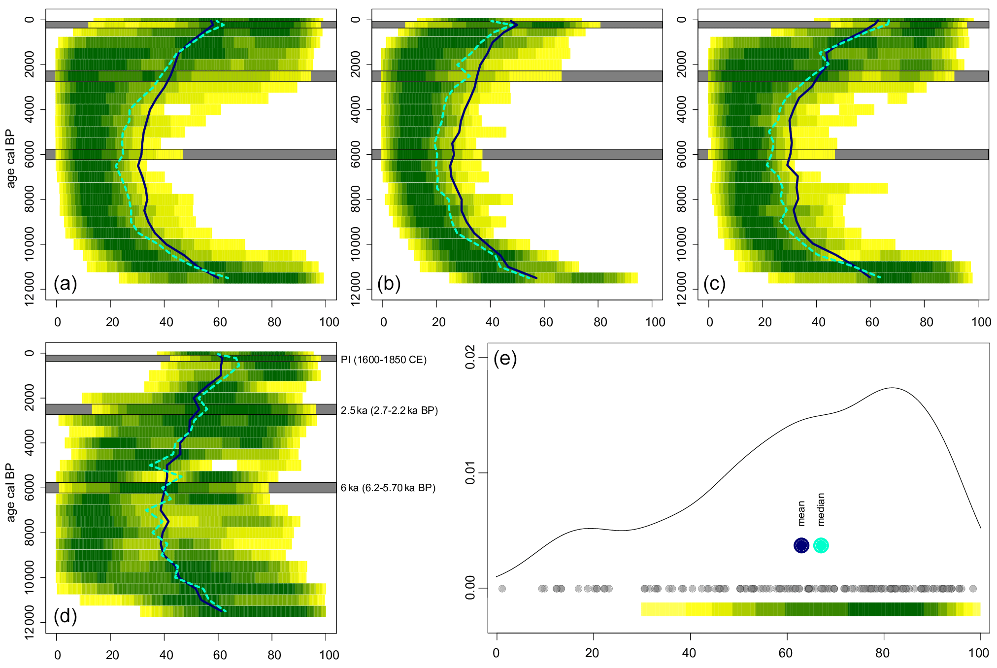
Figure 1 Density plots of REVEALS-based open land (% cover) for (a) all European grid cells, (b) the boreal zone, (c) temperate Europe, and (d) Mediterranean Europe. Full black lines represent the mean value of open land cover, and dashed green lines represent the median value. Panel (e) is illustrative of how the density plots are derived for one time window, showing data values for all grid cells (opaque grey circles), the derived density function as a curve and expressed on the colour gradient, and the mean and median values. Key time intervals (6, 2.5 ka, and the PI period) are highlighted on panels (a–d) by the grey bars.

The period around 6 ka is used by palaeoecologists and climate modellers as a representative time slice of the Holocene thermal maximum and the start of agriculture in large parts of the world. It is used broadly in model–data comparison to evaluate climate models against palaeoclimate proxy data (e.g. Braconnot et al., 2012) and to understand and explain the “Holocene temperature conundrum” (e.g. Bader et al., 2020). However, a better understanding of the possible impact of land use on the Holocene climate since the start of agriculture requires that times of major change in land use are studied. The time around 3 ka (the Bronze Age) was also pinpointed as the time when “the planet [was] largely transformed by hunter-gatherers, farmers, and pastoralists”, as suggested by an archaeological global assessment of land use from 10 ka to 1850 CE (ArchaeoGLOBE Project, 2019). Nevertheless, this time period has not been studied specifically by the wider palaeoclimate modelling community so far. In this paper, we are testing the following hypothesis: the regional climate of Europe around 2.5 ka was significantly influenced by land use via biogeophysical effects due to changes in the properties of the land surface. From a more general perspective, it is also important to understand the biogeophysical effects of LULCC, given that LULCC is affecting most of the Earth's land surface today (Parmesan et al., 2022). Although landscape management is expected to play a large role in the mitigation of climate warming in the future (Nabuurs et al., 2022), the local impact of such mitigation measures on the regional climate and the net effect of both biogeochemical and biogeophysical effects, in the past as well as today, are still not fully understood or known (e.g. Gaillard et al., 2015). The relative importance of LULCC as a climate forcing factor may be large, particularly in low-emission scenarios (van Vuuren et al., 2011).

2 Models and data

2.1 Model chain

This study builds upon a chain of model simulations (see detailed model descriptions below). First, 2.5 ka and latest pre-industrial (1850 CE, hereafter PI) climate conditions are simulated by the ocean–atmosphere coupled global model EC-Earth using prescribed potential PI land cover (Fig. 2 and Table 1). In this context, “potential” refers to land cover without human intervention. The climate conditions for 2.5 ka are then used to force the dynamic vegetation model (DVM) LPJ-GUESS over the European domain to simulate the potential land cover consistent with the climate, labelled L (2.5 k-L in Table 1). The climate conditions from EC-Earth and the land cover from LPJ-GUESS are used to force the RCMs RCA4 and HCLIM. The RCMs simulate the same periods as the global climate model (GCM) but at higher horizontal resolution and with their physical parameterizations. For each RCM, the model output includes a high-resolution climate simulation for 2.5 ka and the PI period (2.5 k-L and PI in Table 1).

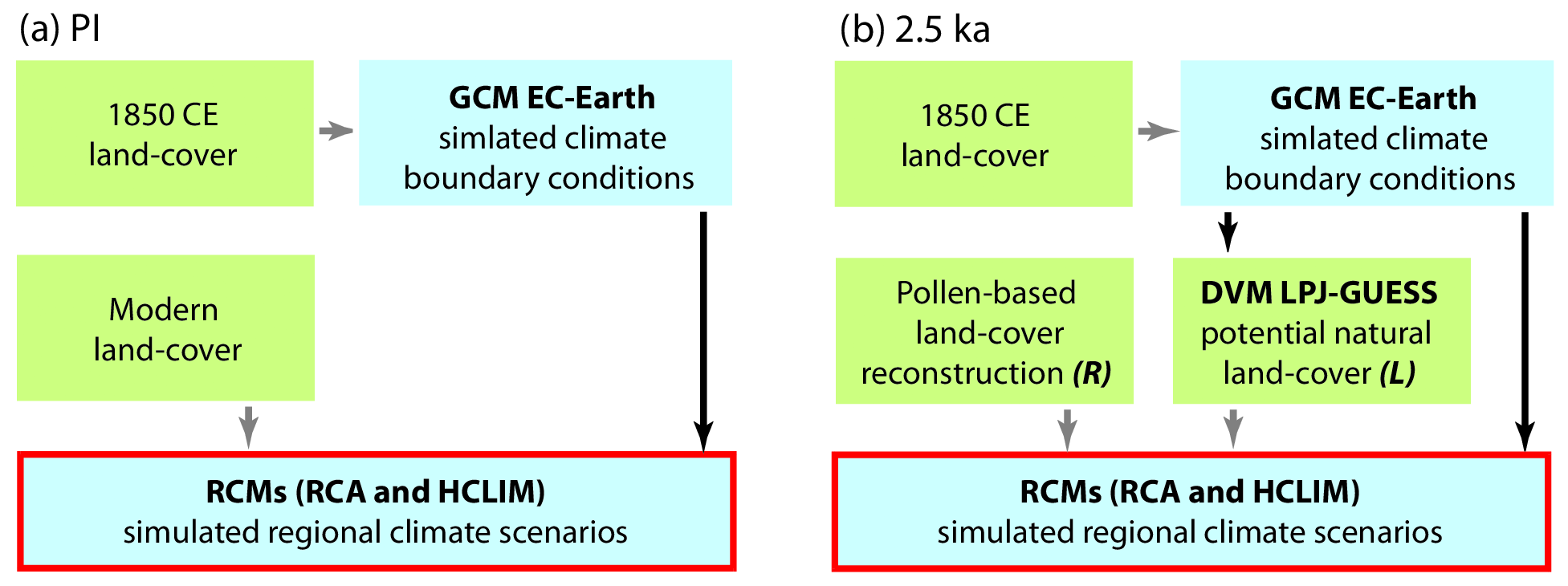
Figure 2 Description of the model chain for (a) the PI period and (b) 2.5 ka. EC-Earth is run for both periods with prescribed potential land cover for the PI period (i.e. 1850 CE). All RCM simulations read boundary conditions from EC-Earth. For the PI period, the RCMs use modern land use. For 2.5 ka, the EC-Earth climate is used in LPJ-GUESS to provide the potential land cover (L) subsequently used in the RCMs. A Bayesian spatial statistical model is used to reconstruct 2.5 ka land cover (R) that is also used in the RCMs (see text for details on the pollen-based reconstruction).

Land cover (i.e. plant cover) at 2.5 ka was reconstructed at a 1^∘ spatial scale using > 1000 pollen records and the REVEALS (Regional Estimates of Vegetation Abundance from Large Sites) model (Sugita, 2007; Githumbi et al., 2022). Because pollen records are not available in all grid cells, a spatial statistics method was used to interpolate the pollen-based land cover over the entire grid covering Europe using the approach described in, e.g. Pirzamanbein et al. (2018). The method uses additional co-variates, i.e. simulated potential land cover from LPJ-GUESS (driven by the climate from the EC-Earth simulation, Fig. 1) and the KK10 LULCC scenario for 2.5 ka (Kaplan et al., 2009). This spatially continuous land cover reconstruction is labelled R (2.5 k-R in Table 1) and represents the climate- and human-induced land cover.

A similar approach was used in Strandberg et al. (2022). Here, we use a more straightforward approach where the LPJ-GUESS simulations use the climate from EC-Earth only instead of also doing an iteration where the RCMs force LPJ-GUESS. Although some studies indicate that more than one iteration between a climate model and the vegetation model are needed to reach equilibrium (e.g. Velasquez et al., 2021), and simulated land cover is sensitive to the representation of climate used and vice versa (Strandberg et al., 2022), we chose to use only one iteration. This is because the difference between reconstructed (based on pollen data) and simulated (based on a vegetation model) land cover is larger than the differences between alternative vegetation model simulations of land cover (Strandberg et al., 2022). Thus, differences in potential vegetation (L) between RCM run iterations would probably not have a large impact on the response to “actual” land cover (R). That response is to a large degree determined by the scale of land cover changes and the climate model used (Davin et al., 2020; Strandberg et al., 2022). Contrasting the simulated potential land cover with the pollen-based reconstruction allows us to explore the effect of LULCC on regional climate. The only difference between the regional climate simulations is the representation of land cover. This would not be possible to achieve with coupled DVM–RCM simulations. Therefore, we catch some of the uncertainty by using the two different land cover representations L and R (Fig. 2). Such sensitivity tests give us the possibility to study the effect of land cover on climate, and how two different RCMs respond to land cover change. The approach also allows us to produce and evaluate a multi-model estimate of 2.5 ka climate.

Table 1 Combination of models and land cover (LC) used in each simulation. EC-Earth is used as the driving GCM in all simulations. The DVM is driven by climate conditions from EC-Earth and simulates potential LC labelled “L”.

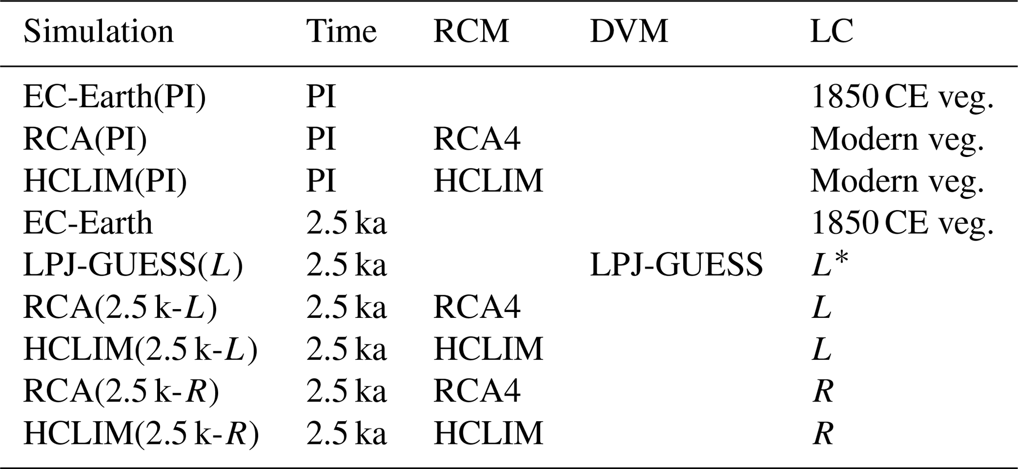
^* The LC is simulated and not a forcing. PI indicates the pre-industrial period (1850 CE). R indicates an interpolated pollen-based REVEALS land cover reconstruction (see Sects. 2.1 to 2.5 for further explanations).

2.2 EC-Earth3.3

The lateral boundary conditions for the RCMs are taken from simulations with the CMIP6 version of the fully coupled general circulation model EC-Earth (Döscher et al., 2022) at T159 horizontal spectral resolution (approximately 1.125^∘ × 1.125^∘) in the atmosphere (this particular configuration is named EC-Earth3-LR in CMIP6, where LR stands for low resolution). The performance of EC-Earth3 when simulating past climate change is evaluated in Zhang et al. (2021). More details on the set-up used here are given in Strandberg et al. (2022).

We perform PI and 2.5 ka simulations following the PMIP4 protocol (Otto-Bliesner et al., 2017). The model setup is described in Zhang et al. (2021). For the 2.5 ka simulation, the climate forcing factors that differ from the PI period are orbital parameters and concentrations of carbon dioxide (CO₂) and methane (CH₄). The orbital forcing for the PI period and 2.5 ka is calculated following Berger (1978). The CO₂ concentrations are 284.2 ppmv (PI) and 276.2 ppmv (2.5 ka), and those for CH₄ are 808.2 ppbv (PI) and 590.6 ppbv (2.5 ka). All other climate forcing factors (e.g. aerosols) and boundary conditions (i.e. land–sea mask, orography) are the same in the PI period and 2.5 ka. The land cover used in the PI and 2.5 ka simulations is prescribed using simulated potential land cover for 1850 CE from LPJ-GUESS implemented offline. The quasi-equilibrium representing the 2.5 ka climate conditions is reached after 200 years of simulation. Note that this LPJ-GUESS simulation is not part of the model runs performed specifically for this study (for more details, see Zhang et al., 2021). Because the choice of vegetation plays a role in the resulting simulated PI and 2.5 ka climates, it will in turn have an impact on the comparison between the PI and 2.5 ka climates. However, the expected climate response of using actual rather than potential PI vegetation in the EC-Earth simulations is much smaller than the difference in climate between the PI period and 2.5 ka. Strandberg et al. (2014) show a response to anthropogenic land cover (instead of potential land cover) at 0.2 ka of maximum +0.5 ^∘C. Therefore, we assumed that the choice of PI vegetation (either potential or actual) in the EC-Earth simulations should not affect the simulated 2.5 ka vegetation or climate to such a degree that it would significantly influence the difference in climate between 2.5 ka and the PI period. Moreover, given that the major focus of our paper is on the difference in the 2.5 ka simulated regional climate when either potential vegetation or actual pollen-based vegetation is used in the RCMs runs, we considered the use of the same potential land cover in the EC-Earth climate runs for both the PI period and 2.5 ka would have little impact on the boundary conditions used for the RCMs runs at 2.5 ka BP.

2.3 RCA4 and HCLIM

Two regional climate models (RCM) are used to downscale the simulations from EC-Earth, thereby adding geographical details and improving the simulation of climatic processes as the horizontal grid spacing is denser in the applied RCMs (∼ 50 km) than in EC-Earth (∼ 100 km). In this study, the Rossby Centre Atmosphere model (RCA4, Strandberg et al., 2015; Kjellström et al., 2016) and the HCLIM38-ALADIN (HCLIM, Belušić et al., 2020) are run on a horizontal grid spacing of 0.44^∘ (corresponding to approximately 50 km) across Europe (the CORDEX EUR-44 domain, Jacob et al., 2014). They have different model physics and cannot be expected to respond to LULCC in the same way. Both RCMs have been extensively used for simulations of past and future climates. RCA4 and HCLIM were used in the same set-up to simulate 6 ka climate (Strandberg et al., 2022). Details on model parameterizations and how the RCMs read data from EC-Earth can be found in that study.

The PI period and 2.5 ka are represented by 30-year periods in the RCMs. Differences in temperatures and heat fluxes between the L and R simulations are tested using a student's t test with a Bonferoni (1936) correction for multiple tests. Accounting for multiple tests is important to reduce the risk of incorrect conclusions when testing for effects across all grid cells (Wilks, 2016). The resulting procedure has a 5 % family wise error rate (FWER), i.e. the probability of one or more false positives among all grid cells is 5 % instead of the 5 % false positive rate for each grid cell obtained when no correction is applied. An alternative would be to use a procedure that corrects for the fraction of false positives, i.e. the false discovery rate (FDR) (e.g. Benjamini and Hochberg, 1995). However, FWER tests are more conservative compared to the FDR alternatives. Only significant differences are shown in Figs. 7, 8, and 10.

2.4 LPJ-GUESS

The dynamic vegetation model (DVM) LPJ-GUESS (Lund–Potsdam–Jena General Ecosystem Simulator) used in this study is an individual-based ecosystem model optimized for regional studies (Smith et al., 2001, 2014; Sitch et al., 2003). LPJ-GUESS has previously been used with RCA3 (Kjellström et al., 2010; Strandberg et al., 2011, 2014) and RCA4 and HCLIM (Strandberg et al., 2022) for different past climates. LPJ-GUESS shows good performance when simulating potential land cover in Europe (Lindgren et al., 2021).

LPJ-GUESS simulates the potential land cover for Europe at 2.5 ka using climate forcing (temperature, precipitation, and radiation) from EC-Earth, and the same CO₂ level as applied in EC-Earth. The land cover input to the RCM is generated by summing the plant functional types into three land cover types: summer-green trees (ST), evergreen trees (ET), and open land (OL) (Table A1). The fraction of the non-vegetated area (or bare land, BL) was estimated by subtracting the summed land cover from 1.

2.5 Pollen-based REVEALS estimates of plant cover and their spatial interpolation

REVEALS (Regional Estimates of Vegetation Abundance from Large Sites) is a model that estimates regional plant cover using pollen records (Sugita, 2007). To achieve reconstructions of past land cover that can be used in climate modelling, pollen-based REVEALS estimates of plant cover are produced at a 1^∘ grid scale using all suitable pollen records available in each grid cell (Gaillard et al., 2010, 2018). The first REVEALS reconstruction of this kind was performed for Europe (Trondman et al., 2015) and was used to evaluate the LULCC scenarios KK10 and HYDE (Kaplan et al., 2017) and discuss the effect of LULCC on simulated regional climate in Strandberg et al. (2014). For this study and the earlier one on the climate at 6 ka (Strandberg et al., 2022), we increased the coverage of the REVEALS reconstruction southwards to the Mediterranean area and eastwards to western Russia and the Middle East (Githumbi et al., 2022). Because the REVEALS estimates of plant cover are not obtained for all grid cells, it is necessary to perform an interpolation to produce a complete pollen-based land cover at a 1^∘ resolution across Europe. This interpolation applies a spatial statistical model described in Pirzamanbein et al. (2018).

The spatial interpolation uses large-scale features consisting of elevation and the LPJ-GUESS land cover fractions adjusted by LULCC at 2.5 ka as derived from the KK10 scenarios (Kaplan and Krumhardt, 2011). The correlation between these large-scale features and the REVEALS estimates of plant cover is computed and used for interpolation. It is important to note that by estimating correlations only the patterns in the features are used for interpolation. The effect on the interpolation of using large-scale features (i.e. LPJ-GUESS land cover) derived from different climate models was small in a sensitivity study (Pirzamanbein et al., 2020), which suggests that a single iteration between the climate model and the vegetation model is sufficient for the spatial interpolation described here. Small-scale spatial patterns in the REVEALS estimates that are not captured by the large-scale features are interpolated by a Gaussian Markov random field (Lindgren et al., 2011). The model uses Dirichlet distributions for compositional data (Aitchison, 1986) to ensure that the interpolated land cover fractions are between 0 and 1 and that the total land cover in each grid cell sums to 1.

The REVEALS reconstructions and the spatial interpolation provide land cover for vegetated areas, with total land cover summing to 1. To account for bare land (BL), the statistical interpolation is adjusted using the fraction of bare ground in the simulated potential land cover obtained from LPJ-GUESS.

To compare the potential and reconstructed land cover used in the simulations, we computed differences between each land cover class for each pixel and joint measures of distance between the complete land cover compositions for each pixel. Let p_k and q_k be the proportions of land cover in the four different classes, indexed by k, for the potential and reconstructed land cover in single pixels. The distances between the two compositions were computed using standard Euclidian distances as follows:

$$\begin{array}{}\text{(1)}& D=\sqrt{{\sum }_k{\left(p_k-q_k\right)}^{\mathrm{2}}},\end{array}$$

and using the compositional distance suggested in Aitchison (1992) and Aitchison et al. (2000) as follows:

$$\begin{array}{}\text{(2)}& \mathrm{ACD}=\sqrt{{\sum }_k{\left(\log \left({\displaystyle \frac{p_k}{\sqrt[K]{{\prod }_l{p}_l}}}\right)-log\left({\displaystyle \frac{q_k}{\sqrt[K]{{\prod }_l{q}_l}}}\right)\right)}^{\mathrm{2}}},\end{array}$$

where K in the root is the total number of classes (K=4 here).

Compared to the Euclidian distance, the Aitchison compositional distance (ACD) puts greater emphasis on relative differences between compositions. As an example, if the land cover fractions change from 40 % evergreen, 20 % summer-green, 20 % open land, 20 % bare land to 49 %, 17 %, 17 %, and 17 %, respectively, the relative abundance of the last three classes stays the same (they are each one-third of the remaining land cover), and the ACD will correctly account for this. As a consequence of this focus on relative differences, an increase from 1 % to 2 % will be seen as very similar (but not identical) to an increase from 10 % to 20 % (both represent a doubling of that composition). Thus, the ACD shows larger differences for areas where one or more compositions are very rare.

3 Results

3.1 Potential and reconstructed land cover at 2.5 ka

Below, potential land cover (L) is the climate-induced land cover at 2.5 ka simulated by LPJ-GUESS using the EC-Earth-derived climate. Reconstructed land (R) is the interpolated pollen-based REVEALS-estimated plant cover, i.e. both climate- and human-induced land cover (Fig. 2 and Table 1).

Potential land cover (L) is dominated by evergreen trees (ET) in northern and eastern Europe (Fig. 3). Summer-green trees (ST) prevail in western Europe, and mixed evergreen and summer green woodland (ET + ST, orange colours) occupy the hemiboreal zone (between the boreal and temperate biomes), starting in southern Norway and becoming more dominant eastwards over southern Sweden, the Baltic countries, and Russia, and an area in the lowlands north of the Alps that meets the hemiboreal zone in Poland. Most mountainous areas of southern and central Europe (Alps, Carpathians, Caucasus) have higher ET proportions than the surrounding plains. At high elevations and latitudes, the Scandinavian mountains are characterized by a higher proportion of open land cover (OL) and bare land (BL) than at lower elevations and latitudes at the expense of trees. Besides those areas, OL proportions are negligible in most of northern and central Europe. OL, often with high BL proportion, has its largest proportions on the western fringe of Europe and in the southeastern part of the continent.

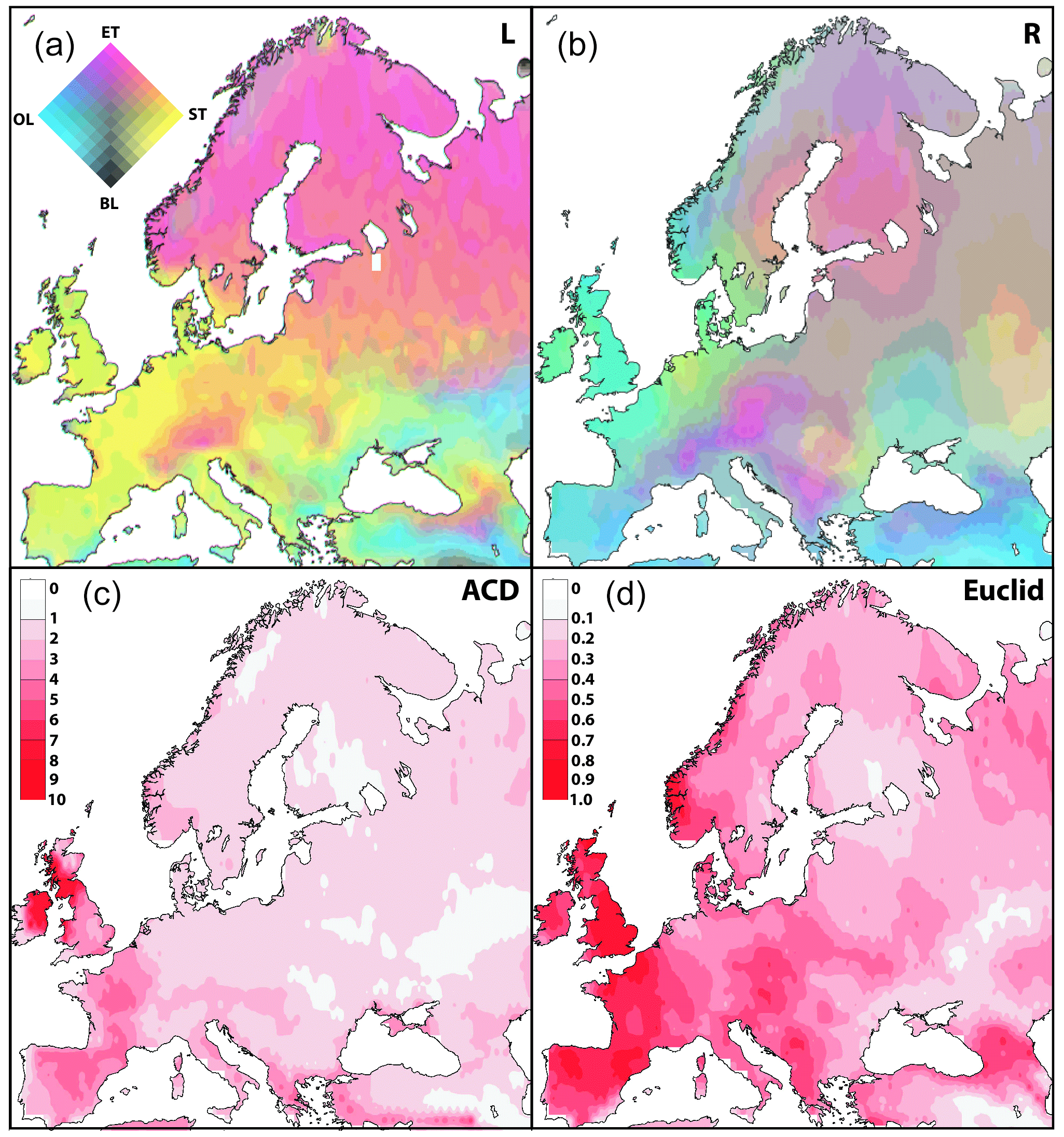
Figure 3 (a–b) Composite maps of (L) LPJ-GUESS-simulated potential land cover using climate input from EC-Earth and (R) interpolated pollen-based REVEALS-estimated land cover in Europe at 2.5 ka. The legend is as follows: ET stands for evergreen trees, ST stands for summer-green trees, OL stands for open land, and BL stands for bare land. (c–d) Two measures of the difference between the composite maps L and R: Aitchison's compositional distance (c) and Euclidian distance (d). The darker the red, the greater the difference in land cover composition between the maps. See Sects. 2 and 3 for details.

The reconstructed land cover (R) shows similar spatial patterns of tree cover to those in the potential land cover, with ET dominant in northern Europe and the mountainous areas of northern and central Europe, and ST having its largest proportions at low latitudes in central and western Europe. However, the proportions of mixed ET and ST woodland and ET and ST mixed with OL in the reconstructed land cover (R) are much larger than in the potential land cover (L).

Both standard Euclidian distances (ED) and Aitchison compositional distances (ACD) (Fig. 3) show that the largest differences between R and L land cover are found in the westernmost parts of Europe in westernmost Norway, Ireland, Britain, western France, and northern Spain. ACDs are larger than EDs for areas where one or several land cover types have small percentage cover (Sect. 2.5), which is the case in Ireland and northernmost Britain. In contrast, EDs are larger than ACDs where none of the land cover types have very low percentage cover (most of northern, central, and eastern Europe). Difference maps (R−L) for the three land cover types (ET, ST, and OL), with BL being the same in both R and L (Fig. A1), provide information on which land cover type(s) most influence the differences between R and L. ET cover is smaller in R than in L land cover (−10 % to −40 %) in most of boreal and northernmost Europe, in particular along the Norwegian coast (up to −40 % to −80 %), while it is larger in R than in L (+10 % to +40 %) in the southern part of temperate and Mediterranean Europe and even more so in western Spain, southwestern France, the French riviera, Italy, and an area in eastern Europe from the Czech Republic down to Greece and western Turkey (+20 % to +40 %). ST cover is smaller in R than in L land cover in temperate and Mediterranean Europe, especially in Spain, France, and the British Isles (−60 % to −80 %), while it is larger in R than in L mainly along the coasts of boreal and northernmost Europe (+10 % to +20 %). OL cover is larger in R than in L in most of Europe (mainly +10 % to +40 %; ≥ 40 % in western Europe) except in an area from Hungry down to northern Greece, Bulgaria, Romania, and central Turkey where R−L is around zero or −10 % to −40 %. The largest R−L differences in OL are found in northwestern Spain, northwestern France, the British Islands, and the northwestern coast of Norway (+40 % to +60 (80) %) and in northeastern Greece, central Romania, southern Russia (Volgograd area), and western Kazakhstan (−20 % to −40 %).

3.2 Simulated climate

Figures 4 and 5 show the differences between the simulated 2.5 ka and PI temperature (at 2 m above surface) and precipitation, respectively, in winter and summer. Here we describe the results for the 2.5 k-R runs because they use land cover data inferred from empirical proxies of past land cover; i.e. pollen-based REVEALS estimates of plant cover, which is so far the best possible reconstruction of actual land cover in the past (e.g. Trondman et al., 2015; Kaplan et al., 2017; Roberts et al., 2018; Githumbi et al., 2022). We describe the impact of different land cover data on climate in Sect. 3.3. Henceforth, the difference in temperature or precipitation between 2.5 ka (with land cover R in both RCMs) and the PI period are abbreviated T 2.5 k − PI and P  2.5 k − PI, respectively. Note that the EC-Earth simulations do not use the land cover data R for 2.5 ka but instead use prescribed potential land cover for 1850 CE (see Sect. 2 for more details). As expected, the general similarities between the GCM and the RCMs simulated climates are larger over the ocean, where the model resolution is less important, and smaller over land, where the land surface is treated differently in the GCM and the RCMs.

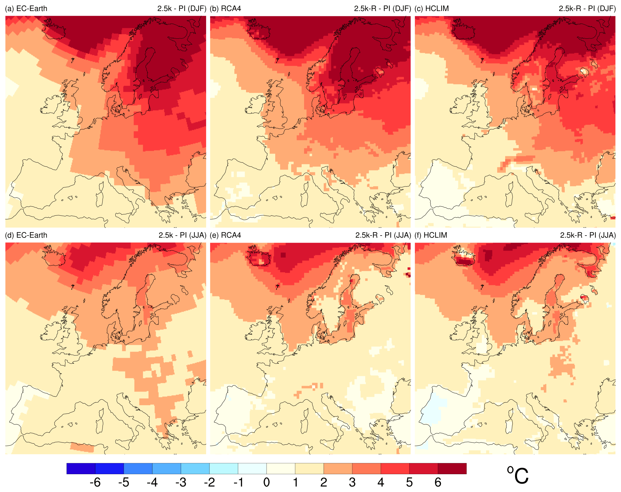
Figure 4 Temperature difference (^∘C) between 2.5 ka and the PI period (T 2.5 k-R− PI) for winter (DJF, a–c) and summer (JJA, d–f) as simulated by EC-Earth (a, d), RCA4 (b, e), and HCLIM (c, f).

In winter, all simulations indicate that 2.5 ka was warmer than the PI period and show a similar pattern, with the smallest temperature differences between 2.5 ka and the PI period (T 2.5 k − PI) on the Iberian Peninsula (0–1 ^∘C) and the largest differences in northeastern Europe (4− > 6 ^∘C) (Fig. 4). The RCMs exhibit similar patterns to EC-Earth, but these are smaller T 2.5 k − PI with ca. 0.5 ^∘C on the Iberian Peninsula. Moreover, HCLIM shows smaller T 2.5 k − PI than EC-Earth and RCA4 in most of central Europe. In summer, the smallest T 2.5 k − PI are also found on the Iberian Peninsula and in western Europe, while the largest T 2.5 k − PI occur in the northern parts of the domain, especially in areas close to the sea–ice margin in the far north (Fig. 4). The difference in T 2.5 k − PI between RCA4 and HCLIM is larger in summer, although patterns are similar. While T 2.5 k − PI is 1–2 ^∘C in the HCLIM simulations, it is close to zero in central and eastern Europe in the RCA4 ones. Both RCMs simulate a T 2.5 k − PI of 0.5 to 1.5 ^∘C in the eastern and northern parts of the domain, which is less than in EC-Earth.

Overall, and in both winter and summer individually, the difference in precipitation between the two time periods (P 2.5 k − PI) is small (within ±10 %), except for areas close to the northern rim of the domain in winter, where 2.5 k-R is wetter than the PI period with P 2.5 k − PI ≥ 50 % in all models (Fig. 5). Most regions in central Europe and the Mediterranean are characterized by low positive or negative P 2.5 k − PI (up to ±10 %). All three models show similar precipitation patterns, which suggests that precipitation is mainly governed by the large-scale circulation as simulated by the driving GCM. However, there are notable differences in P 2.5 k − PI between the RCMs and EC-Earth, which suggests that changes in the precipitation amount also result from local processes including small-scale convection.

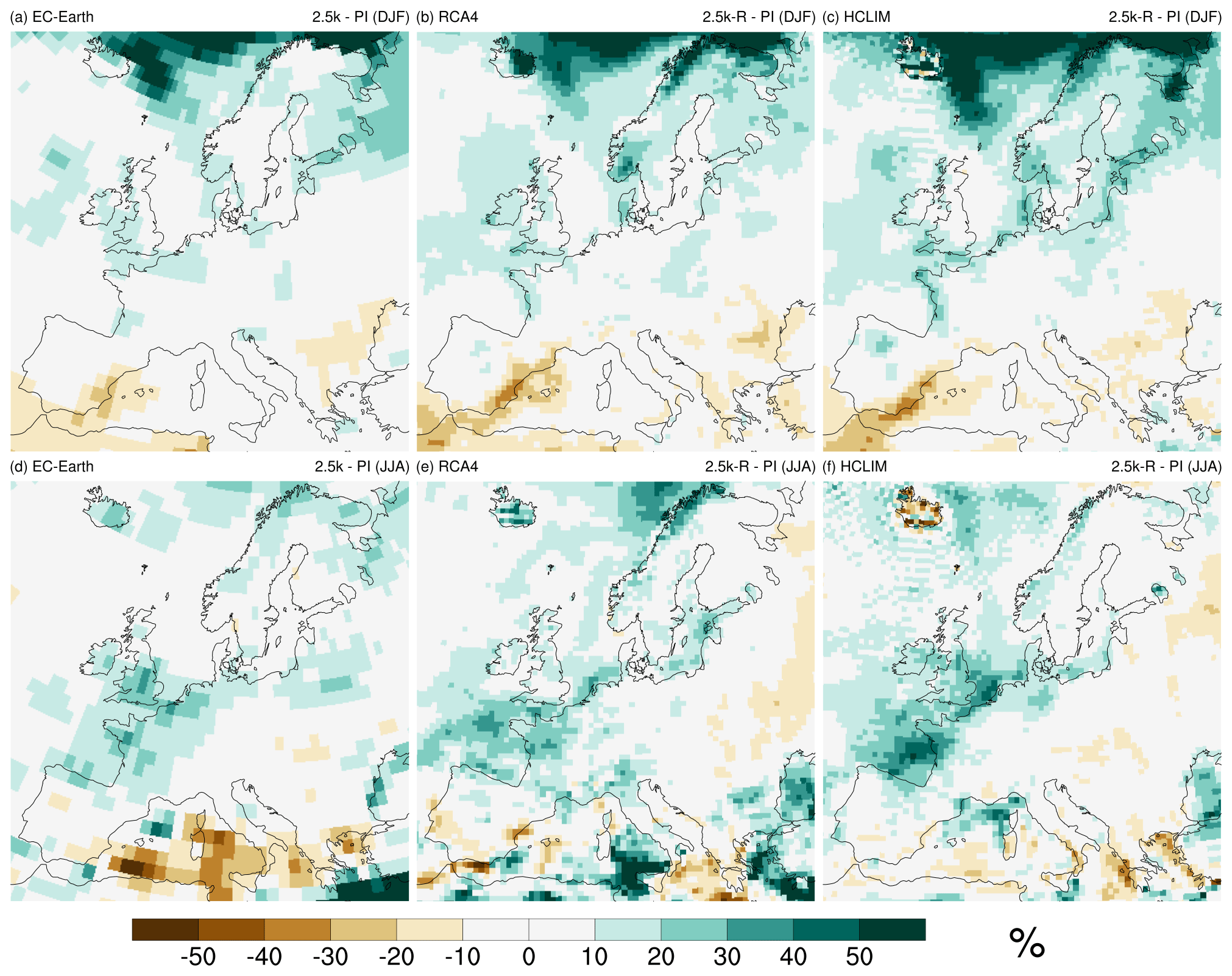
Figure 5 Precipitation difference (%) between 2.5 ka and the PI period with the reconstructed land cover R (P 2.5 k-R− PI) for winter (DJF, a–c) and summer (JJA, d–f) for EC-Earth (a, d), RCA4 (b, e), and HCLIM (c, f).

Figure 6 shows sea level pressure (SLP) at the PI period and the difference between 2.5 ka and the PI period (SLP 2.5 k − PI). In winter, the RCMs show similar patterns to EC-Earth, but these generally show a slightly lower pressure over the continent. Comparing the two time periods, it is clear that SLP is lower at 2.5 ka than at the PI period over Scandinavia, the British Isles, and the North Atlantic, which implies enhanced cyclone activity. Lower SLP values at 2.5 ka than the PI period occur farther south and are more common over Scandinavia in EC-Earth than in the RCM simulations. Such differences between the RCMs and the driving GCM partly explain differences in P 2.5 k − PI between the models and between time periods. For instance, the negative SLP difference in Scandinavia and the North Atlantic may be related to that region's larger positive precipitation difference (Fig. 5).

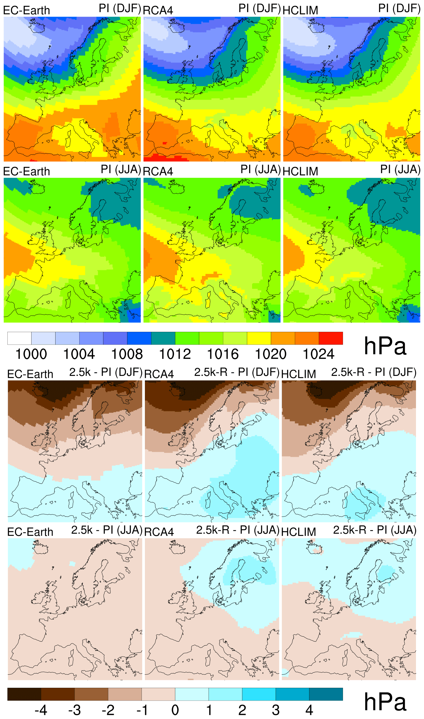
Figure 6 PI sea level pressure (hPa) in winter (DJF, first row) and summer (JJA, second row). Difference in sea level pressure (hPa) between 2.5 k-R and the PI period in winter (DJF, third row) and summer (JJA, fourth row). EC-Earth (left), RCA4 (middle) and HCLIM (right).

In summer, the simulated mean SLP patterns in the PI period are similar between EC-Earth and the RCMs. It is also clear that differences between the two periods (SLP 2.5 k − PI) are generally small, which may contribute to the small differences in precipitation (P 2.5 k − PI) between the periods (Fig. 5). The RCMs show higher SLP at 2.5 k over Scandinavia, as opposed to EC-Earth. Potentially, the lower SLP in EC-Earth may be representative of the positive P 2.5 k − PI in the area east of the Baltic Sea where the RCMs show small, or even negative P 2.5 k − PI.

3.3 Climate response to differences in land cover: the effect of human-induced land cover

Here, the RCM 2.5 k-R runs described in Sect. 3.2 are used as the reference and compared with the 2.5 k-L runs; i.e. Fig. 7 shows the difference in climate at 2.5 ka resulting from changing land cover from the potential (climate-induced) land cover (L) to the pollen-based reconstructed land cover (both climate- and human-induced change) (R) (Fig. 2). The difference is expressed as (2.5 k-R) – (2.5 k-L), which is henceforth abbreviated as R−L (Table 1). Here we present the surface temperature instead of the diagnostic 2 m temperature, the latter being defined in different ways depending on the model (Breil et al., 2020), while surface temperature has a standard definition (Fig. 7).

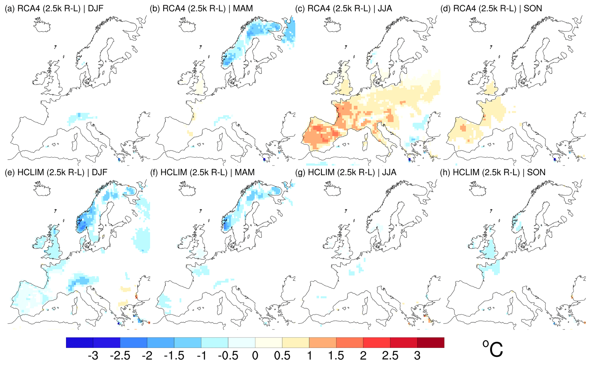
Figure 7 Difference (2.5 k R−L) in surface temperature (^∘C) in RCA4 (a–d) and HCLIM (e–h) for winter (DJF; a, e), spring (MAM; b, f), summer (JJA; c, g), and autumn (SON; d, h). Only grid cells that show a significant difference on a 0.05 level are coloured.

In most of the area, temperature differences are not significant except for some areas, most notably for HCLIM. In winter the R−L temperature differences are negative (−1 to −0.5 ^∘C) over the Alps in both RCMs (Fig. 7a, e). HCLIM simulates larger R−L temperature differences than RCA4 in large parts of Scandinavia and western Europe, suggesting a stronger sensitivity of HCLIM than RCA4 to the difference in land cover data. Also in spring, differences are small. A common feature for both RCMs is that R−L temperature differences are negative (−3 to −1 ^∘C) in large areas of Scandinavia that include a mountain range (Fig. 7b, f).

In summer, RCA4 responds strongly to the inferred land cover differences. The R−L temperature difference is 0.5–2 ^∘C in southwestern Europe (Fig. 7c, g). HCLIM, on the other hand, shows very small R−L temperature differences. The only significant differences are seen over limited regions in western Europe and over scattered points in the Iberian Peninsula and along coastal areas in the southeast.

4 Discussion

4.1 Differences in land cover descriptions

Simulated potential (L) and pollen-based reconstructed (R) land cover exhibit compositional differences (Fig. 3, description in Results). Major differences between LPJ-GUESS-simulated Holocene vegetation and pollen-based REVEALS reconstructions of land cover were discussed in a study using 19 pollen records along N–S and W–E transects through Europe (Marquer et al., 2017) based on pollen-based REVEALS reconstructions of open land cover. Other earlier studies have compared the results of DVM simulations in Europe with pollen accumulation rates and pollen percentages (e.g. Miller et al., 2008) or pollen-based REVEALS estimates of land cover (e.g. Pirzamanbein et al., 2014).

It must be kept in mind that the prescribed simulated climate entirely determines the DVM simulated potential land cover in this study; i.e. the simulations do not account for the effects of LULCC. The reconstructed land cover is a pollen-based reconstruction of the climate- and human-induced land cover, i.e. a product of complex interactions between several natural and anthropogenic factors. Disentangling climate-induced changes from human-induced changes in pollen-based vegetation is a challenge. Marquer et al. (2017) used a novel approach including the use of variation partitioning to quantify the percentage of variation in vegetation composition explained by climate and land use variables. The results suggest that climate is the major driver of vegetation when the Holocene is considered as a whole or at a sub-continental scale, but land use appears to be important regionally. Land use becomes a major control of vegetation from ca. 4.5 ka, although climate is still the principal driver; however, its influence decreases gradually. Land use is the cause of the more or less continuous increase in OL and decrease in ST from ca. 7 ka (southern Europe) and 6 ka (temperate and most of boreal Europe) until 1850 CE (e.g. Marquer et al., 2014, 2017; Githumbi et al., 2022). However, changes in pollen-based OL do not necessarily represent LULCC but may be due to climate-induced land cover changes such as the spread or decrease in open wetland areas as a consequence of water-level changes (e.g. Pinke et al., 2017). Pollen from the plant families Poaceae (grasses) and Cyperaceae (sedge family) are either difficult or impossible to identify to genera or species, which hampers categorization into dry, fresh and wet meadows; i.e. all types of open land, whether natural or human-induced, include large amounts of Poaceae and/or Cyperaceae. Consequently, pollen-based OL cover may overestimate human-induced land cover change. In contrast, cropland (or agricultural land, AL in, e.g. Trondman et al., 2015), also included in OL, is always underestimated in pollen-based AL cover as it represents cereals only. This is because pollen productivity estimates are not available so far for other crops, and/or the pollen grains of many crops are not distinguishable from the pollen of wild species belonging to the same plant genera or families. Further details on the interpretation of OL cover in terms of human-induced vegetation openness can be found in Trondman et al. (2015). Despite these issues, it is assumed that most of the increase in pollen-based OL cover since the start of the Neolithic period is human-induced change and that OL cover before the introduction of agriculture was in general < 20 % (ca. 10 %–20 %; Fig. 1).

Differences between R and L land cover (in addition to those due to LULCC) could be caused at least partly by differences between the actual climate (responsible for the climate-induced part of pollen-based vegetation) and the model-simulated climate. Causes of differences between R and L other than discrepancies in climate and LULCC include processes involved in tree migration (e.g. the Holocene migration lag in Picea and Fagus; see Giesecke and Bennett, 2004; Giesecke et al., 2007, 2017) and soil development (e.g. Miller et al., 2008). Despite continuous progress in effectively modelling such processes in DVMs and ecosystem models, it is not yet implemented as a routine (D. Lehsten et al., 2014; V. Lehsten et al., 2019). Lower ET values in R land cover than in L land cover in most of northern Europe at 2.5 k BP are partly due to overly large abundances of Picea in the LPJ-GUESS simulation. The latter is known from earlier comparisons between LPJ-GUESS-simulated vegetation and records of pollen accumulation rates (Miller et al., 2008) or pollen-based REVEALS reconstructions of plant cover (Marquer et al., 2017) over the Holocene. However, the latest comparison between LPJ-GUESS and REVEALS total tree cover in boreal Europe shows that LPJ-GUESS mean total tree cover (MTTC) is in good agreement with REVEALS MTTC in boreal Europe at 2 ka BP when standard deviation is considered (Dallmeyer et al., 2023). At a subcontinental spatial scale and for the PI period, MTTC is larger in LPJ-GUESS simulations than in REVEALS estimates in the British Isles only, and it is lower in LPJ-GUESS than REVEALS in northernmost Europe and the alpine region. In continental and boreal Europe, the difference in MTTC is insignificant when the standard deviations are considered. The largest disagreement between LPJ-GUESS and REVEALS estimates in large parts of northern Europe is found instead in the relationship between evergreen and deciduous tree cover where LPJ-GUESS simulates larger cover of evergreen trees than their REVEALS-estimated cover (Fig. A1; Marquer et al., 2017).

4.2 Response in the RCMs to land cover changes

The temperature response to different land cover data in winter and spring results from the snow albedo feedback and the insulating impact of the snow cover. Open land generally has a higher albedo than forests. Open land is also more readily covered by snow, which makes the differences in albedo between open land and forest larger during the snow season. Thus, the temperature response is expected to be the strongest in regions of high altitude or high latitude where there is snow in winter and where the fraction of open land is relatively large.

At high latitudes, the amount of incoming solar radiation is small in winter, making the snow albedo response weak. The only model consistent R−L temperatures in winter are seen over the Alps. In the Scandinavian mountains, the snow season is long, stretching through spring. Here, the temperature response is stronger in spring when the amount of incoming radiation is larger, even though the difference in albedo between 2.5 k-R and 2.5 k-L is smaller in spring than in winter (Fig. 7a, b, e, f; see also Fig. 9). The response in temperature to land cover differences is coherent with the differences in albedo in winter (Fig. 8a, b). The differences in albedo closely follow the differences in land cover, since land cover to a large extent determines albedo. This agrees with earlier studies of idealized land cover changes in RCMs showing that albedo explains a large part of the temperature signal in winter in Scandinavia (Strandberg and Kjellström, 2019; Davin et al., 2020). Note that differences in albedo can be small but still significant because the variability is small. Some of the differences in the range of ±0.1 in Fig. 8a and b are < 0.05 and should not be considered different from zero (i.e. no difference).

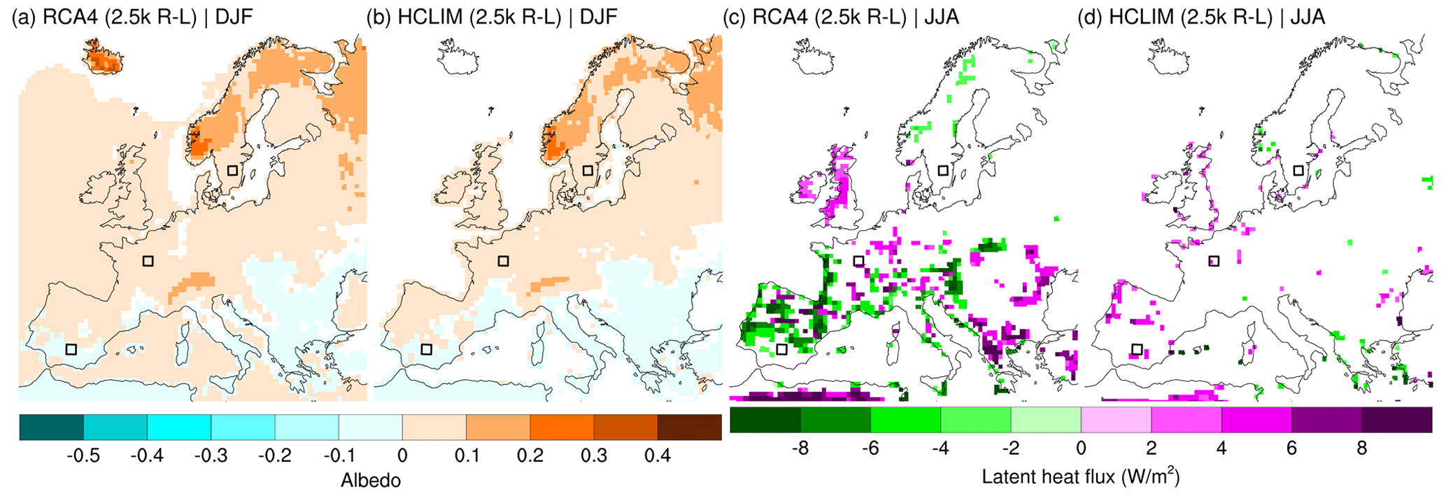
Figure 8 Difference between 2.5 k-R and 2.5 k-L in albedo in winter (DJF) for (a) RCA4 and (b) HCLIM and in latent heat flux in summer (JJA) for (c) RCA4 and (d) HCLIM. Black squares show the areas representing Scandinavia (SCA), western central Europe (WCE), and the Iberian Peninsula (IBP). Only grid cells that show a significant difference (p<0.05) are coloured.

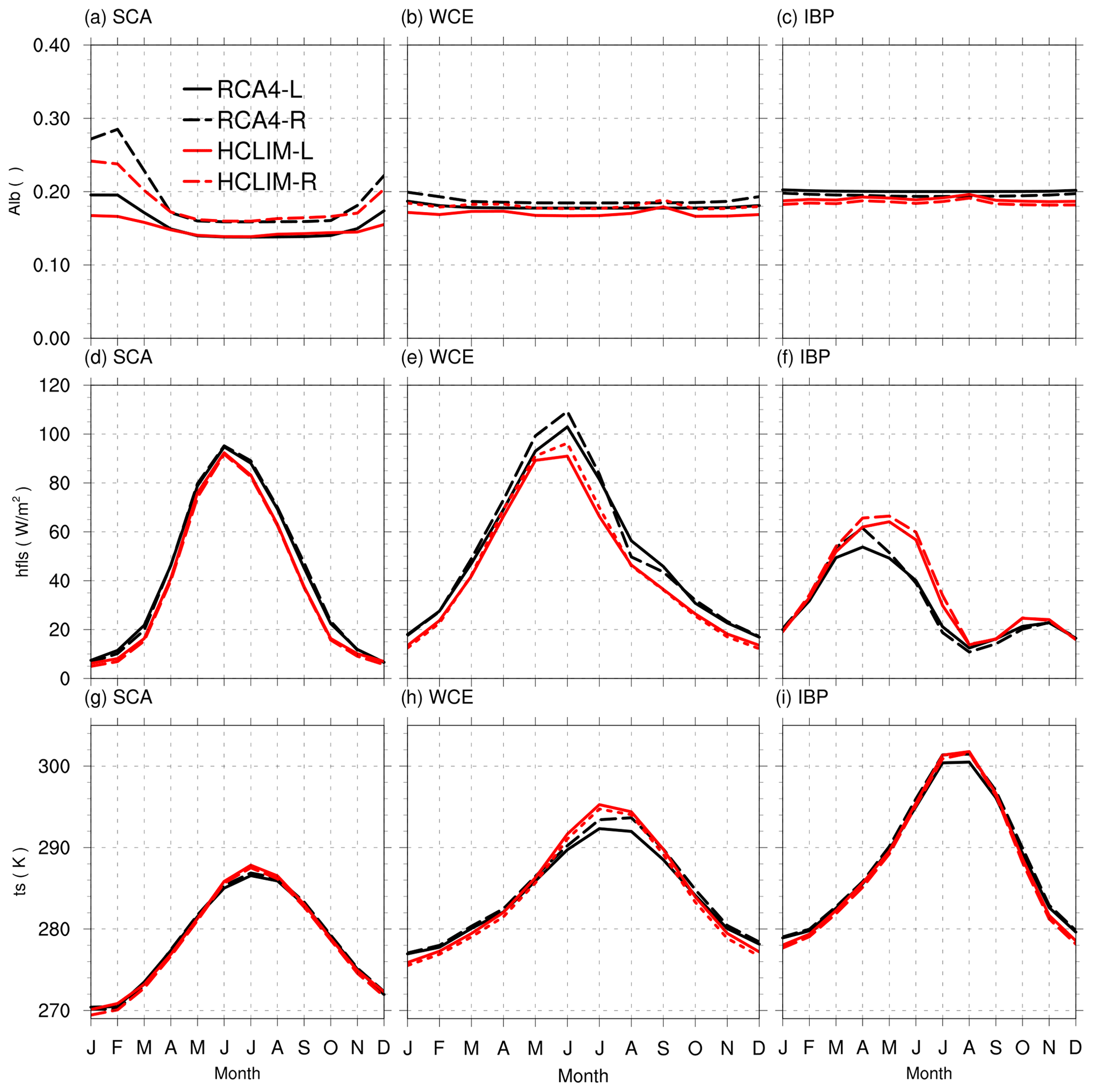
Figure 9 Annual cycles of surface albedo (alb; a–c), latent heat flux (hfls (W m⁻²); d–f) and surface temperature (t_s (K); g–i) for Scandinavia (SCA; a, d, g), western central Europe (WCE; b, e, h), and the Iberian Peninsula (IBP; c, f, i). Data from RCA4 are represented by black lines, and data from HCLIM are represented by red lines. Simulations using potential land cover from LPJ-GUESS are labelled with “L” and shown as full lines, and those using pollen-based REVEALS reconstructed land cover are labelled with “R” and shown as dashed lines.

The areas with the largest R−L temperature differences in summer (Fig. 7c, d, g, h) correspond to the areas with the largest significant differences in latent heat flux as simulated by RCA4 (Fig. 8c). Trees have deeper roots and more leaves than grass, which implies more evapotranspiration (EVT). A more open landscape, such as 2.5 k-R, is expected to be warmer in summer due to decreased EVT. In contrast, HCLIM shows few significant temperature differences as a result of very small differences in latent heat flux (Fig. 8d). Davin et al. (2020) demonstrated that RCMs could disagree in their temperature response to idealized changes in land cover in summer. There is not a direct relationship between differences in land cover and simulated changes in EVT. EVT is determined in the models by the magnitude of land cover differences, as well as the absolute amount and type of vegetation. Furthermore, local conditions, such as available soil moisture, determine how much water is available for EVT. How these factors are translated into temperature responses depends on the individual models' physics and parameterizations.

The roughness length (Z₀) is also changed by LULCC; therefore, differences in Z₀ could potentially explain some of the climatic responses. As Z₀ differences are constant over the year, the same scale of vegetation changes would give the same Z₀ difference across the domain. Consequently, roughness changes cannot explain why the response to LULCC is different depending on the season or the region. We consider albedo and latent heat flux the most likely explanations because they best correlate with temperature differences.

To better understand the relationships between surface albedo, latent heat flux, and temperature, we present the annual cycles in absolute values for three different small regions (3 × 3 grid points) representing Scandinavia (SCA), western central Europe (WCE), and the Iberian Peninsula (IBP) (regions shown in Fig. 8). Overall, all four simulations (RCA4 and HCLIM with R or L land cover) agree in terms of shape and amplitude of the annual cycles (Fig. 9). The largest discrepancies between RCA4 and HCLIM are found in the annual cycles of EVT in WCE and IBP. In WCE, RCA4 simulates a larger amplitude and slightly higher values of EVT in the second half of the year. In IBP, it is HCLIM that simulates a larger amplitude and a longer period of high EVT. Trees have a longer period of EVT than herbs but not necessarily a higher annual maximum of EVT (Kelliher et al., 1993; Strandberg and Kjellström, 2019). Resulting differences are seen for WCE and IBP in RCA4 and to some extent HCLIM simulations. A possible explanation for the higher latent heat fluxes in the 2.5 k-R runs is that grasslands do not retain water as efficiently as woodlands, which would mean that the latent heat flux increases faster and reaches higher levels to then drop faster. Such a pattern is seen in both RCA4 and HCLIM simulations, but it is clear that RCA4 tends to dry out more rapidly than HCLIM (Fig. 9f).

4.3 RCM-simulated climate compared to proxies

To evaluate the climate model simulations, we compare simulated temperatures to proxy data from the Temperature 12k database (Kaufman et al., 2020a). We let all proxy data represent the overall patterns of 2.5 ka temperature and compare those with the overall patterns from the models. Figure 10 shows winter and summer temperatures at 2.5 ka as given by proxy data and the climate models with R land cover in this study.

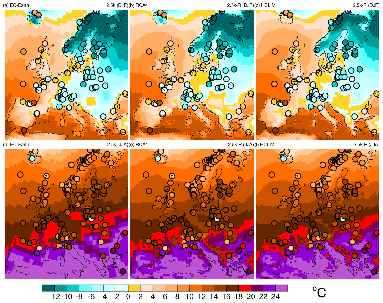
Figure 10 Temperature (^∘C) at 2.5 ka in winter (DJF, a–c) and summer (JJA, d–f) as simulated by EC-Earth (a, d), RCA4 (b, e), and HCLIM (c, f). Proxy data are shown as circles.

In winter, there is a general agreement among the models that temperatures range, along a northeast to southwest gradient, from −10 ^∘C and below in northeastern Europe to around 5 ^∘C in the Iberian Peninsula. There is also agreement that eastern Europe is colder than western Europe at the same latitudes and that the Scandes, the Alps, and the Carpathians are colder than the surrounding areas. Compared to proxies, the models are colder in Iceland (except perhaps HCLIM) and warmer along the coasts of western Europe and in parts of central and eastern Europe. In summer, there is a general agreement that temperatures range from around 10 ^∘C in the north to approximately 24 ^∘C in the south. Compared to proxies, the models are warmer in Iceland and central eastern Europe, especially in EC-Earth.

Even though there is general agreement between models and proxies, there are also differences. Some proxies show considerable differences to the model data, and even if proxies and data have the same colour in Fig. 10, the difference may be up to 2 ^∘C. In addition, the proxy temperature data are not internally consistent, which makes it difficult to evaluate their utility in data–model comparisons. The proxy data come from lake sediment, marine sediment, peat, glacier ice, and other natural archives, and temperatures are inferred with different methods and have varying uncertainties (Kaufman et al., 2020a). There is also a problem with the spatial scale of the reconstructed versus simulated climate. Proxy data may represent local climate conditions that do not necessarily match the spatial scale of the model simulated climate. Making an in-depth model–proxy comparison would require an assessment of each data point (what they represent, uncertainty ranges, etc.) that is outside the scope of this paper. Future studies could improve the model–proxy comparison, for example by compensating for differences in altitude between model and proxy data (e.g. Strandberg et al., 2011). For this study, it is sufficient to conclude that the models give a picture of 2.5 ka temperatures that largely agrees with that from proxy data.

To decide whether the inclusion of reconstructed land cover improves the comparison with proxy data, we compare each proxy data point with the value from the corresponding grid cell in all four RCM simulations. Figure 11 shows how the proxy data correlate to the simulated temperature in HCLIM in winter and summer. The general agreement between models and proxies seen in Fig. 10 is also seen here as fairly strong correlations in both winter and summer. The differences between HCLIM-L and HCLIM-R are small, both the root-mean-square error (RMSE) and the correlation coefficient are more or less the same for both simulations (Table 2). RCA4 and EC-Earth also give similar values.

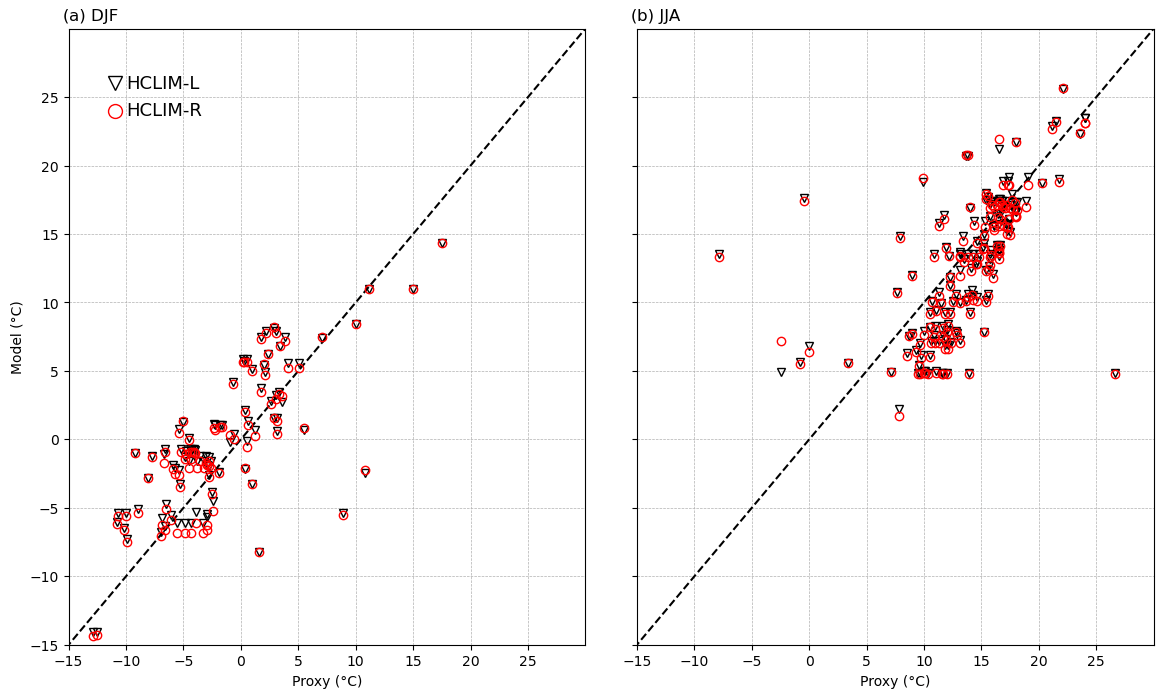
Figure 11 Simulated (y axes) and proxy (x axes) temperatures at 2.5 ka in winter (a) and summer (b). Temperatures from HCLIM-L are represented by black triangles, and those from HCLIM-R are represented by red circles. The locations of the data points are seen in Fig. 12.

Table 2 Correlation (Corr.) and root-mean-square error (RMSE, ^∘C) between simulated 2.5 ka temperatures and proxy temperatures.

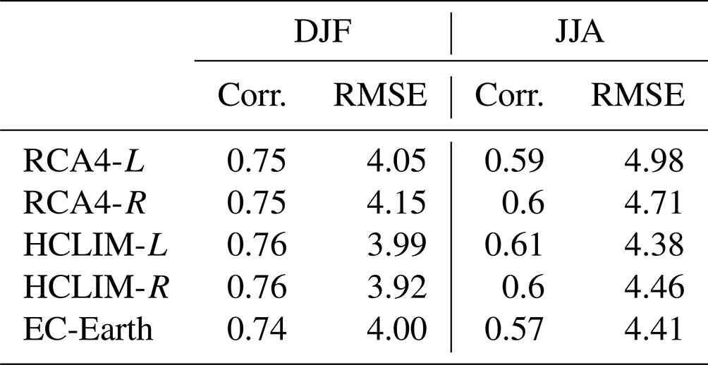
It is a challenge to assess the effect of adding human-induced land cover on simulated climates in comparison to having climate-induced land cover only, since the uncertainties in climate proxy data are large and the land-cover-induced differences in climate are small compared to the absolute temperatures and temperature differences due to other forcing (e.g. Strandberg et al., 2011). Moreover, the model–data comparison (Fig. 11; Table 2) is hampered by the irregular spatial distribution of climate proxy data. They do not represent the entire European domain and are often missing in the regions where the largest differences between L and R simulations are suggested by our results. Several sites are located along the coast or in the ocean. Even if we consider only the points in regions where we suspect large differences, such as Scandinavia in winter and western Europe in summer, the conclusion is the same. The climate proxy dataset at hand do not have the necessary spatial distribution to assess whether the inclusion of human-induced land cover improves the simulated climate or whether the RCMs improve simulated regional climate compared to the GCM EC-Earth (Table 2).

4.4 Robustness of the results

The natural variability in Europe is large (e.g. Deser et al., 2020), which influences the comparison between 2.5 ka and PI climates. Three adjacent 30-year periods in EC-Earth, considered here to represent the studied 2.5 ka climate, differ by up to 1 ^∘C. A wider description of the 2.5 ka climate, including natural variability, would require ensemble simulations including more time slices. The difference in climate between 2.5 ka and the PI period is a result of orbital forcing and greenhouse gas concentrations (Singh et al., 2023). Since our model experiment does not include sensitivity runs changing one forcing at a time, we do not know which forcing plays the largest role.

The large-scale climate conditions as represented by the driving GCM are important for the RCM-simulated regional climate (e.g. Rummukainen, 2010). The dependence of GCM-simulated changes in large-scale circulation on precipitation in the RCMs is a well-known feature seen in projections of future climate change (e.g. Kjellström et al., 2018; Christensen and Kjellström, 2020). In addition, different GCMs and/or different simulations with the same GCM reflecting natural variability tend to yield large regional differences (e.g. Deser et al., 2020). For instance, natural variability alone may explain a large part of differences between models and why one model study differs from another or from reconstructions using proxy data.

Even with identical forcing, the response to regional differences in land cover can differ significantly between model simulations. The response in several RCMs (of which RCA4 was one) to idealized land cover changes was studied for present climate conditions (Breil et al., 2020; Davin et al., 2020). They showed large agreement across models in the temperature response to albedo in winter. In summer the analysed RCMs showed different signals in the response to heat flux and temperature. Russo et al. (2022) suggest that this could be explained by how the land surface scheme works in the individual model and how sensitive they are to, e.g. perturbations in soil moisture. The small response in latent heat flux and temperature in HCLIM in summer relative to that in RCA4 shows that sensitivity to land cover changes differs across models, regions, and seasons; however, it is not necessarily a sign of conflict or disagreement between models. Larger land cover changes may trigger a similar response in both RCA4 and HCLIM, although testing this would require a series of simulations with incrementally larger land cover changes, and these tests have not been performed.

Consequently, using other models would have given different results. We acknowledge that we only represent a small part of the total uncertainty and that a larger variety of climate models and/or initial conditions representing natural variability would enable a better assessment of these differences. Our way of handling model uncertainty is to use two models with different model physics. As we get a similar response to that obtained in studies of idealized climate–land cover interactions using idealized land cover forcing studies under present climate conditions (Strandberg and Kjellström, 2019; Breil et al., 2020; Davin et al., 2020) and comparable studies of past climate (Russo et al., 2022), we ascribe most of the uncertainty associated with the response to differences in land cover in our study to differences in the two models' physics. To improve the estimate of uncertainty in our results will require larger multi-model ensembles. Such ensembles are not available for 2.5 ka to date.

5 Conclusions

This study describes the climate and land cover 2500 years ago (at 2.5 ka) as simulated by one GCM, two RCMs, and one DVM and using one reconstruction of 2.5 ka land cover based on pollen data, statistical interpolation methods, and climate model results. The results provide some insights into how simulated climate is influenced by LULCC and how sensitive RCMs are to differences in land cover.

The results presented here suggest that LULCC at 2.5 ka impacted the climate in parts of Europe. Simulations including LULCC give up to 1 ^∘C higher seasonal mean temperature in parts of northern Europe in winter and up to 1.5 ^∘C warmer temperatures in southern Europe in summer than simulations with potential land cover. This relatively strong response suggests that anthropogenic land cover changes may have affected European climate during the Bronze Age. This also implies that LULCC is important in future scenarios, especially in low-emissions scenarios where the greenhouse gas forcing is relatively small.

The models simulate a 2.5 ka climate that was warmer than the PI climate, as a result of different orbital forcing and feedbacks. The largest differences are seen in northern Europe, where the 2.5 ka climate is 2–4 ^∘C warmer than the PI period. In summer, the difference between the simulated 2.5 ka and PI climates is smaller (0–3 ^∘C), with the smallest differences in southern Europe. Differences in precipitation are mostly within ±10 %. In parts of northern Europe, the climate at 2.5 ka is up to 30 % wetter in winter than that of the PI period. In summer, there is a tendency for the 2.5 ka climate to be drier than the PI period in the Mediterranean region.

Two different forest types dominate the simulated potential land cover at 2.5 ka: evergreen coniferous forests in northern and eastern Europe and deciduous broadleaved forests in western Europe. The portion of open land cover is negligible in all forested areas and dominates only in the steppe region of southeastern Europe. Reconstructed land cover, however, shows mixed forests in most of Europe. Furthermore, there is a high portion of open land in forested regions, and, in addition to the steppe region, open land cover dominates in most of western and southern Europe. Altogether the reconstructed land cover is considerably more open than the simulated potential land cover in most of Europe.

The choice of land cover has a significant impact on the simulated temperature. Winter and spring temperatures are closely related to albedo, which is largely the same in both RCMs and is strongly affected by land cover. In summer, the RCMs used in this study respond somewhat differently to land cover differences, showing that the choice of land cover and climate model is important for the resulting simulated climate. Summer temperatures are strongly related to differences in heat fluxes between the atmosphere and the ground. Since the response in heat fluxes to differences in land cover depends on model physics, it is more likely that models respond differently in summer than in winter. For summer, RCA4 responds more strongly to the imposed differences in land cover than HCLIM. This explains some differences between the climate conditions simulated by RCA4 and HCLIM. It is difficult to assess which model has the most realistic response. Model performance is dependent on many other factors including, but not limited to, large-scale circulation, parameterizations, and resolution. The best way to understand this model uncertainty is to use multi-model ensembles to capture the range of possible climates.

The importance of model and land cover choice calls for caution when designing palaeoclimate experiments. Here we show that it is essential to have a good, well-motivated description of land cover to simulate the same climate with different models in a model ensemble.

Appendix A

Table A1 Groups of land cover types used in this study.

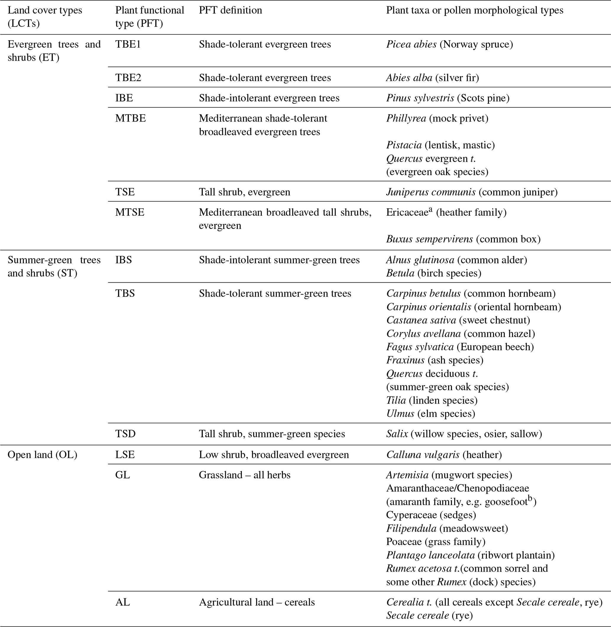
^a Ericaceae (MTSE): the pollen productivity used for Ericaceae pollen in the REVEALS reconstruction represents the mean pollen productivity of several species of which Arbutus unedo, Erica arborea, E. cinerea, and E. multiflora are dominant. The genus Calluna vulgaris (heather, LSE) also belongs to the Ericaceae family, but its pollen productivity has been estimated separately (Githumbi et al., 2021). Cerealia t.: all cereals except Secale cereale (rye) that are easily separated on the basis of pollen morphology and for which pollen productivity was estimated separately.
^b The most recent plant taxonomy has merged the family Chenopodiaceae into the family Amaranthaceae, i.e. “new” Amaranthaceae represents “former” Amaranthaceae + Chenopodiaceae. Pollen analysts have mostly used the name Chenopodiaceae for this pollen morphological type, but it includes all species from the two former families, therefore the name Amaranthaceae/Chenopodiaceae.

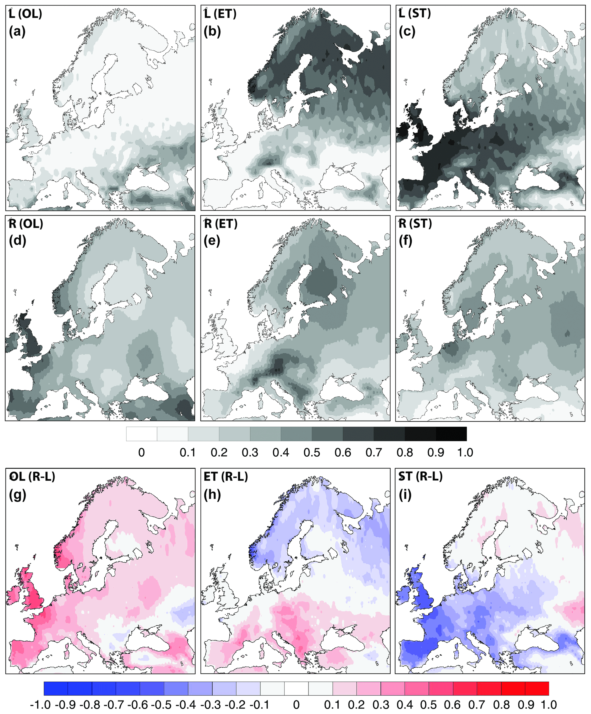
Figure A1 (a–f) Cover (in fraction of grid cell) of open land (OL), evergreen trees (ET), and summer-green trees (ST) at 2.5 ka in Europe as (a–c) simulated by LPJ-GUESS using climate input from EC-Earth (L) and (d–f) estimated using pollen data and the REVEALS model (R). (g–i) Difference between L and R cover (R−L). See Sects. 2 and 3 for details.