the Creative Commons Attribution 4.0 License.
the Creative Commons Attribution 4.0 License.
 | 20 Jun 2023
Viticulture extension in response to global climate change drivers – lessons from the past and future projections
Nicolas Bernigaud
Alberte Bondeau
Laurent Bouby
Wolfgang Cramer
The potential areal extent of agricultural crops is sensitive to climate change and its underlying drivers. To distinguish between the drivers of past variations in the Mediterranean viticulture extension since Early Antiquity and improve projections for the future, we propose an original attribution method based on an emulation of offline coupled climate and ecosystem models. The emulator connects the potential productivity of grapevines to global direct and indirect climate drivers, notably orbital parameters, solar and volcanic activities, demography, and greenhouse gas concentrations. This approach is particularly useful to place the evolution of future agrosystems in the context of their past variations. We found that variations in potential area for viticulture during the last 3 millennia in the Mediterranean Basin were mainly due to volcanic activity, while the effects of solar activity and orbital changes were negligible. In the future, as expected, the dominating factor is the increase in greenhouse gases, causing significantly drier conditions and thus major difficulties for viticulture in Spain and North Africa. These constraints will concern significant areas of the southern Mediterranean Basin when global warming exceeds +2 ∘C above preindustrial conditions. Our experiments showed that even intense volcanic activity comparable to that of the Samalas – sometimes considered to be the starting point of the Little Ice Age in the mid-13th century – would not decrease aridity and so not slow down this decline in viticulture extension in the southern margin of the Mediterranean area. This result does not confirm the idea of geoengineering that solar radiation modification (SRM) is an efficient option to limit future global warming.
- Article
(13412 KB) - Full-text XML
- BibTeX
- EndNote


Our scientific question is related to the attribution of viticulture, which has had an economic role in the Mediterranean Basin since antiquity, extension changes to any natural or anthropogenic drivers. The cultivation and domestication of the grapevine began between the 7th and 4th millennia before the common era (BCE) between the eastern Mediterranean and Caspian areas and spread to Egypt, the Middle East, and the entire Mediterranean (Terral et al., 2010; Bouby et al., 2021). Introduced in the Gaul region (i.e., roughly France and surrounding regions) by Greek colonists ca. 600 BCE, around the time they settled Marseilles, viticulture was initially limited to Mediterranean Gaul (Bouby et al., 2014). Vineyards expanded into the northern part of Gaul in the 1st century CE, where wine production developed quite considerably in the following centuries up to the Paris region, the Rhine and Moselle valleys (Brun, 2010), and even in southern England (Brown et al., 2001). One hypothesis behind this expansion is the climate warming during the Roman Climatic Optimum (RCO) (Mccormick et al., 2012). These climate variations are driven by global forcing variables such as solar or volcanic activity (Wanner et al., 2008; Brayshaw et al., 2010; Fuks et al., 2017). After the RCO, the temperature decreased significantly and Gaul entered the so-called Late Antique Little Ice Age, or LALIA (536–660 CE) (Büntgen et al., 2016). This change may have been triggered by several large volcanic eruptions at 536, 540, and 547 CE (Sigl et al., 2015). This assumption remains difficult to prove because of the limited historical and archeological sources. In any case, the 500 to 900 CE period remained relatively cold with oscillating precipitation changes in the region (Reale and Dirmeyer, 2000). In Europe, the following Medieval Climate Anomaly (MCA, approx. 900–1200 CE) (Luterbacher et al., 2016) was likely of intensity comparable to the RCO. The Little Ice Age (LIA, approx. 1250–1850 CE) was a period of alpine glacier advance (Holzhauser et al., 2005), again marked by several large volcanic eruptions, in particular that of the Samalas (Indonesia) in 1257 (Lavigne et al., 2013).
On timescales of centuries and millennia, quality and yield of agricultural crops are strongly affected by climate fluctuations. The nature of the change depends on external forcings and internal feedbacks of the climate system, which produce different spatial and seasonal patterns of the main variables in the atmospheric environment. The main objective of this paper is to develop an innovative solution to statistically model the impact of changing climate forcing on vegetation over several millennia using the grapevine (a major crop of the Mediterranean and European region) as an example. We mimic this impact model on the basis of a large ensemble of existing model simulations using statistical relationships much faster to compute (Kennedy and O'Hagan, 2000). Based on a large range of climate states from high-resolution simulations with coupled Earth system models for the last glacial period to future global warming scenarios, this approach, called a “emulator”, provides robust results and can be applied to a large range of ecosystem processes under different conditions.
The global drivers of the studied changes are anthropogenic, including greenhouse gas (GHG) emissions, land use and cover changes, population density, and economic production, and natural, including the Earth's orbit as well as volcanic and solar activity. They are the boundary conditions of Earth system models (ESM) (Kay et al., 2014). The ecosystem processes are assessed using impact models (IMs) coupled to these ESMs (Franklin et al., 2016; Warszawski et al., 2014; Frieler et al., 2017). In most cases, coupling is offline because (i) the spatial scales of ecosystem processes are much finer than are those of ESMs, thus making a scale transfer necessary (Su et al., 2016); (ii) a climate simulation of a given ESM is interpreted as one realization out of a set of possibilities determined by the boundary conditions and the characteristics of the ESM, thus making it necessary to work on ensembles of models to be representative of the climate system (Kay et al., 2014); and (iii) each ESM has intrinsic biases that must be corrected before it can be used to drive the ecosystem model (Williamson et al., 2015).
Even if human innovation and colonization were also responsible for the expansion of viticulture, the climate must be suitable for grape cultivation and thus remains a control variable. As soon as the climate changes to worse conditions for wine growth, it becomes a driver of a decline in viticulture. Such fluctuations are particularly noticeable near the northern range limit of wine growth during the end of the Roman and Medieval periods with a regression of the grape cultivation.
Although we focus our viticultural analysis on the Gaul region (France and surrounding countries), we need to enlarge the area to the entire Mediterranean and European surrounding region to robustly capture the relationships between global drivers and viticulture extension. For the same reason, we use a large diversity of time slices of the past (Last Glacial Maximum, mid-Holocene, last millennium) and of the future up to 2100 according to several scenarios. The widely diverse situations used for calibration made it possible to produce a robust emulator that was effective for extrapolating a wide range of past and future climate states. This method is appropriate to establish a bridge between past variations of a given agrosystem and its future evolution. Once calibrated, the emulator is of great help to efficiently support decisions in the domain of impacts of climatic change.
As ESMs are an imperfect representation of reality, our approach has the same limitations even if the model parameters are carefully chosen (Crucifix, 2012). Crucifix (2012) developed the idea that a Bayesian framework is adequate to stimulate the modeling of the distance between the ESM and reality. So ESMs produce a certain vision of the world that needs to converge to the reality represented by the paleodata. This procedure is called data assimilation, which provides a way to reduce the uncertainties.
The concept of our method and the data used are presented in Fig. 1. Global forcings are the inputs of low-resolution ESMs. Step 1 involves adapting output fields to a common high-resolution grid using statistical downscaling. This step is also useful to correct the systematic biases of the ESM simulations. Step 2 involves applying the vegetation model BIOME4 to the high-resolution fields to calculate ecosystem variables. Steps 1 and 2 are repeated for each ESM simulation available. These simulations based on different forcings and different models provide a large and diversified calibration dataset. They are a guarantee that the emulator is in some way more robust than the ESM simulations taken separately. Calibration of the emulator (step 3) is done by spatial regression of the ecosystem variables on the forcing variables. Step 4 involves the application of the emulator to the forcings of new time slices or future scenarios. During this step, the annual temperature and precipitation results for the past time slice were compared to paleodata to identify the amplitude of the volcanic and solar activity effects (data assimilation). Step 5 is the independent validation of the emulator using tree-ring data.
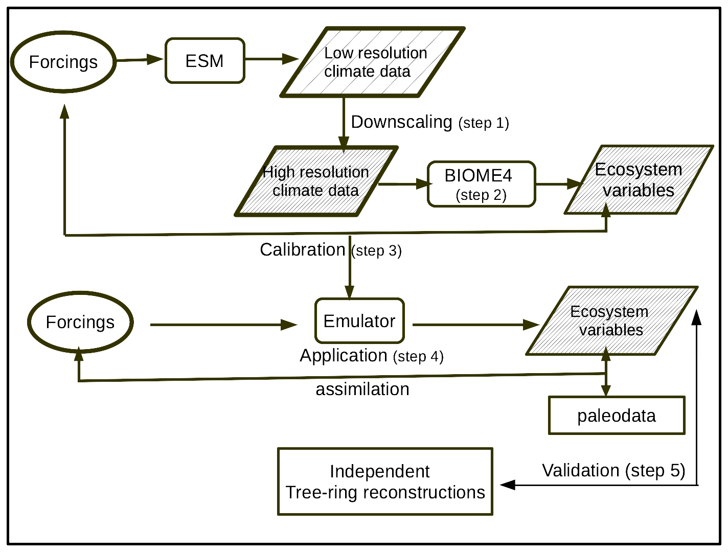
Figure 1Diagram of the different steps in the emulator approach; the ecosystem variables, related to bioclimate and net primary productivity, are defined in Table 1. Low-density hashes in the trapezes indicate low resolution of the corresponding data, and high-density hashes correspond to higher resolution.
Table 1The biome types simulated by BIOME4 and output variables used for the paper; note that there is no correspondence between the two columns.
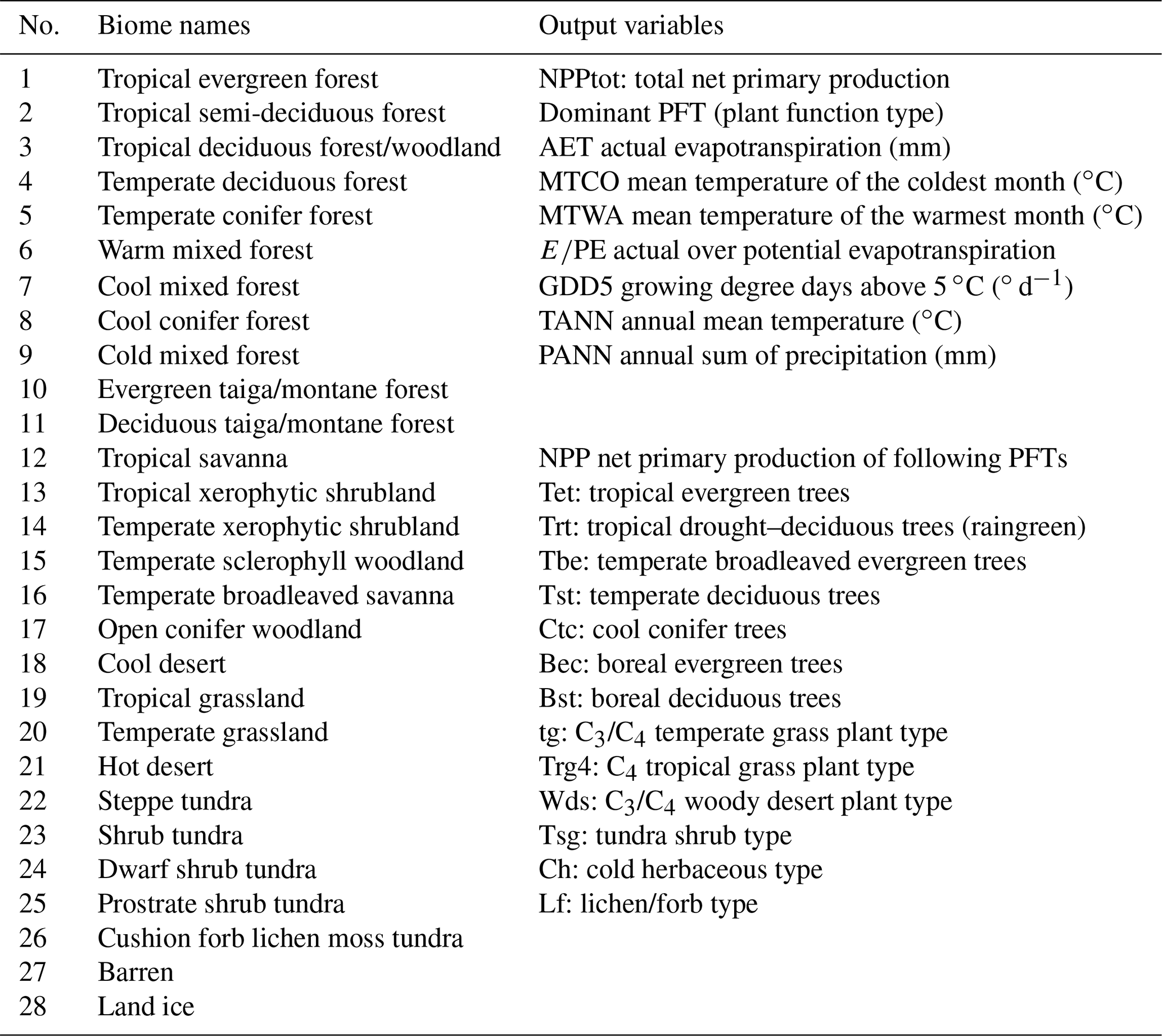
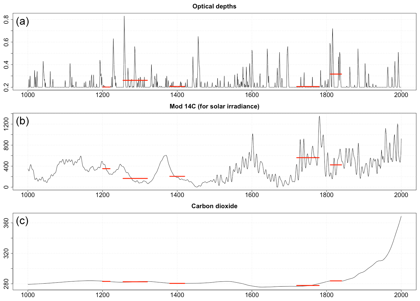
Figure 2Natural (volcanic activity and solar activity) and anthropogenic forcing (CO2) for the last millennium: (a) the effective aerosol radius, which is directly related to the aerosol optical depth, is calculated by Crowley and Unterman (2013); (b) the proxy indicating the total solar irradiance (TSI), i.e., the solar modulation function in MeV based on 14C (Muscheler et al., 2007); and the (c) atmospheric CO2 concentration (in ppm). The red horizontal lines represent the mean values of the five selected periods.
2.1 The forcing variables
Climate forcings or drivers are perturbations imposed on the Earth's energy balance. They are mainly the following.
- i.
Orbital parameters: eccentricity (ecc) and obliquity of the ecliptic (obl) as well as solar longitude at the perihelion (ω), or more precisely the climate precession pr = ecc × sin (ω). Nevertheless, to avoid redundancy, we use as forcing variables the three basic parameters (ecc, obl, ω). They drive the orbit of the Earth and influence its climate by modulating the solar energy intercepted by the planet and its seasonal distribution at timescales above thousands of years (Berger and Loutre, 1991). They had a major impact on the Earth's climate from the last glacial period to the Holocene. At the century timescale, the orbital parameters do not operate significantly, so the values of the last millennium can be linearly interpolated between the values at 1000 yr BP and the present values, and the values of the 21st century can be set to the present values.
- ii.
Greenhouse gas (GHG) concentration: carbon dioxide (CO2), methane (CH4), and nitrous oxide (N2O). The effect of these GHGs has been significant from the glacial to interglacial periods and has a major effect for the current century (see, for example, Fig. 2 for CO2).
- iii.
The world population values taken from the Hyde 3.1 database for the past periods from Klein Goldewijk et al. (2011) and for the future periods from van Vuuren et al. (2011). The population varied from less than 106 at the Last Glacial Maximum (LGM) to 7×10⁹ in 2010 and is projected to be between 9×10⁹ and 12.3×10⁹ in 2100 according to the scenario.
- iv.
Volcano activity (V) represented by the effective aerosol radius deduced from the aerosol optical depth from ice core sulfate records from both polar regions for the last millennium (Crowley and Unterman, 2013) (Fig. 2). Its value is 0.2 when there is no eruption. The maximum value (0.8) was found in 1258, the year after the Samalas eruption (Lavigne et al., 2013). The 21 ka, 6 ka, and future values were set to the preindustrial values.
- v.
Solar activity (S) is inferred from 14C and 10Be records, the proxy for the total solar irradiance (TSI) (Muscheler et al., 2007) for the last millennium, and varies from 0 to 1200 MeV (Fig. 2). The 21 ka, 6 ka, and future values were set to the preindustrial values.
2.2 The past time climate data (used for calibration)
The past time periods retained for calibration are (1) the Last Glacial Maximum (21 ka) characterized by very low greenhouse gases (GHGs), low ecc, and obl and a pr close to zero determined by a low ecc; (2) the mid-Holocene (6 ka) characterized by GHG close to that of the preindustrial period, low ecc and pr, and a large obl increasing the seasonality of the climate; (3) five periods of the last millennium (Fig. 2) representing various combinations of S and V forcings, including V− S+ (1200–1220), V+ −S (1255–1320), V− S+ (1380–1420), V− (1720–1780), and V+ S+ (1810–1840); and (4) the preindustrial (PI) reference period with intermediate GHG concentrations, low ecc, medium obl, medium pr, and large V and S.
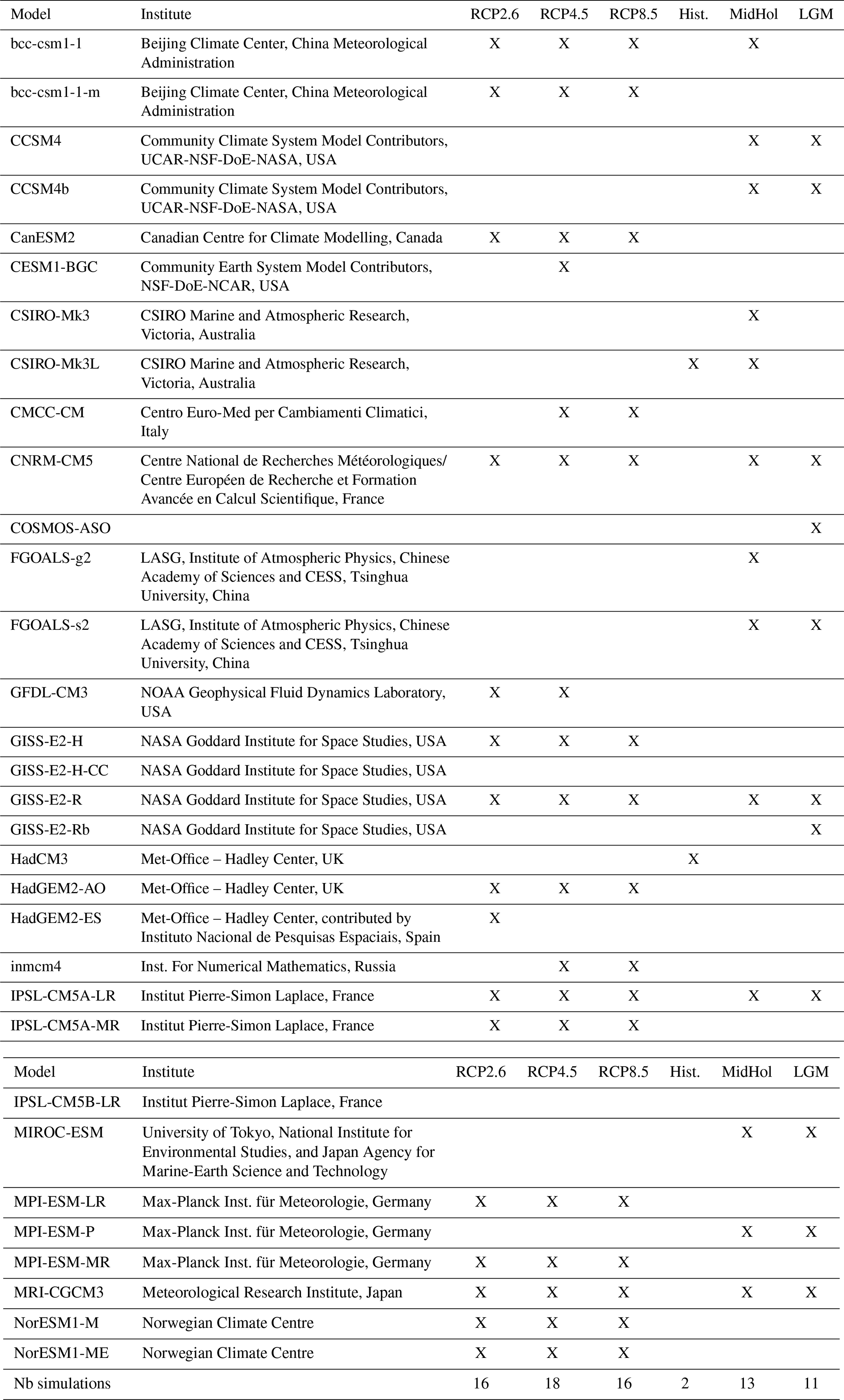
The simulations were archived by the Paleoclimate Modelling Intercomparison Project (PMIP), which produced snapshot simulations of the mid-Holocene (6 ka BP) and Last Glacial Maximum (21 ka BP) time slices to study the effects of insolation, greenhouse gases, and massive ice sheets on the climate (https://pmip3.lsce.ipsl.fr/overview/, last access: 15 June 2023) (Braconnot et al., 2012). The models used for intercomparisons were coupled atmosphere–ocean–vegetation models with various levels of complexity and resolution (Table 2).
Table 2CMIP5 and PMIP3 simulations used in the paper. The first column is the code of model, and the second indicates the institute which built the model; the other columns provide the availability of the scenarios (RCP) or time slices. Hist.: historical period (last millennium), MidHol: mid-Holocene (6 kyr BP), LGM: Last Glacial Maximum (21 kyr BP).
2.3 The future climate data (used for calibration)
The future periods are determined by increasingly high GHG concentrations (depending on the scenario, see below), and the other forcing variables were set to the PI value. The simulations were archived by the Coupled Model Intercomparison Project (CMIP). We used simulations of CMIP5 (Taylor et al., 2012). These include both (i) century-scale integrations, which usually start from a preindustrial control, and climate predictions until the end of the 21st century, as well as (ii) near-term integrations for the next 10 to 30 years, which are initialized using observed ocean and sea-ice conditions. The CMIP5 climate change projections are driven by emission scenarios divided into four classes referred to as Representative Concentration Pathways (RCPs) (Moss et al., 2010). The high-emissions scenario, named RCP8.5 or “business as usual”, refers to a high radiative forcing of emissions at the end of the 21st century (8.5 W m−2). The low-emission scenario, which roughly represents that of the Paris Agreement, reaches its maximum value near the middle of the century before decreasing to a level of 2.6 W m−2 at the end of the century. We only used the intermediate scenario RCP4.5, which refers to a radiative forcing maintained at values of 4.5 W m−2 at the end of the 21st century. We used 10 time slices interpolated at a 10-year steps (2010, 2020, …, 2100). The forcing variables for the future scenarios were obtained from the website http://tntcat.iiasa.ac.at/RcpDb/ (last access: 15 June 2023).
2.4 The application data
We used our emulator to analyze the response of key ecosystem variables to global forcing. We focused on past periods that were marked by important climate and societal changes (Table 3). The present time slice was defined by the mean values for the 1961–1990 period. For the future, instead of using time slices, we defined the scenarios according to the global temperature signal simulated in the different models using the relationship between global warming and CO2 concentration (Guiot and Cramer, 2016).
- i.
The +1.5 ∘C global warming recommended by the Paris Agreement is reached with a CO2 concentration of 440 ppm; Fig. 3 shows that the average model simulation reaches this value under scenario RCP2.6 in approximately 2040.
- ii.
The +2 ∘C global warming is reached with a CO2 concentration of 480 ppm and is reached under scenario RCP4.5 in approximately 2050 (Fig. 3).
- iii.
The +3 ∘C global warming is reached with a CO2 concentration of 600 ppm and is reached under scenario RCP8.5 in approximately 2060 (Fig. 3).
- iv.
The +5 ∘C global warming is reached with a CO2 concentration of 900 ppm and is reached under scenario RCP8.5 in about 2090 (Fig. 3).
We obtained the corresponding CH4 and N2O concentrations and population sizes from the boundary condition database of CMIP5. The other future forcings are set to the present values.
Table 3Typical past periods used to calibrate our emulator. The paleoclimatic and societal information is found in the literature given in the references from the late Holocene to the present.
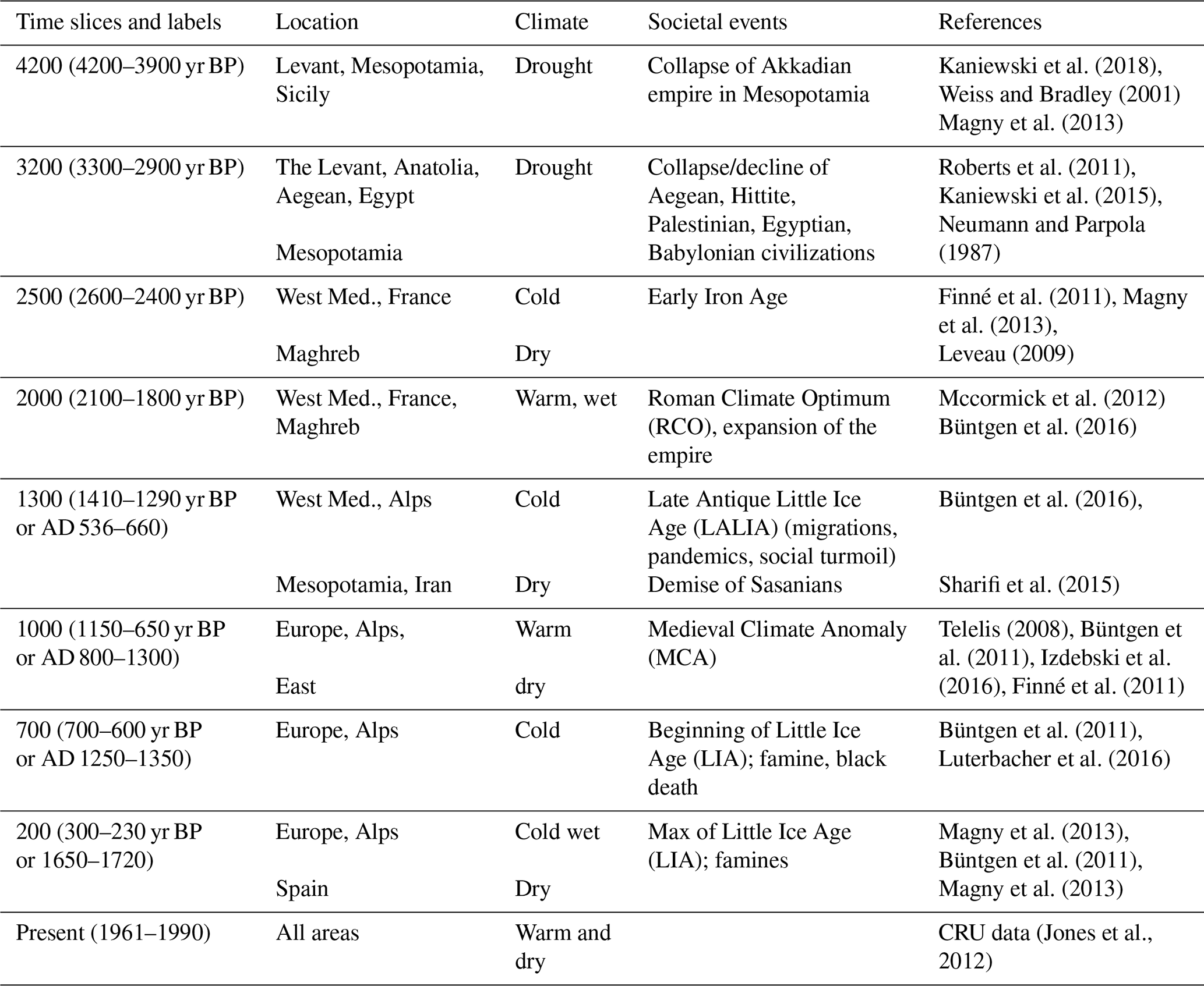
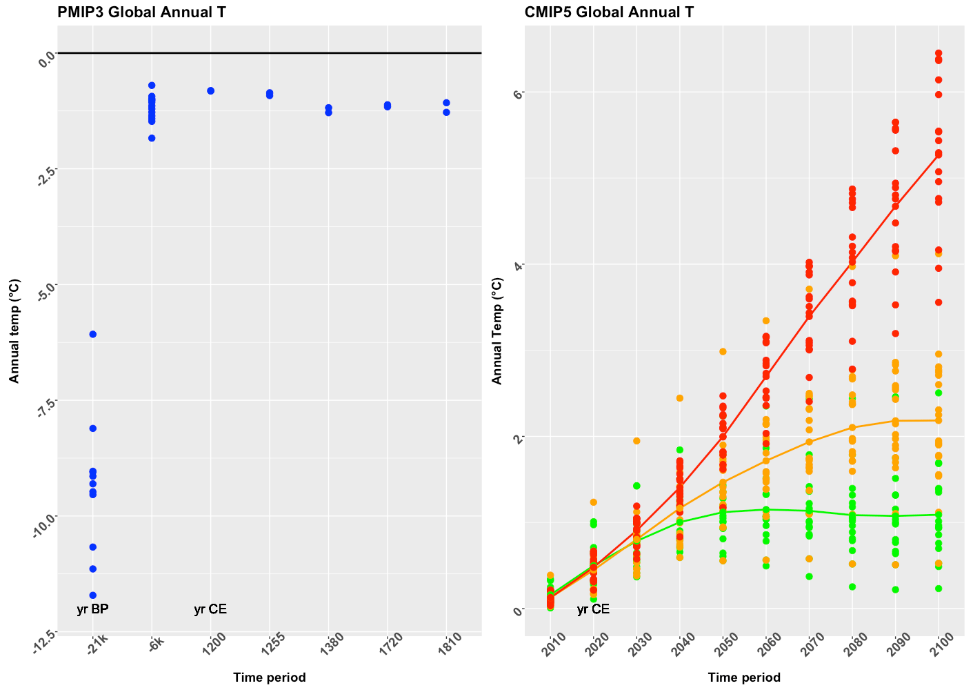
Figure 3Global annual temperature anomalies (T) simulated by the various models of PMIP3 and CMIP5, according to the reference period average (1961–1990). The left graphic represents the past simulations, and the right graphic represents the present and future projections for three scenarios (RCP2.6 in green, RCP4.5 in orange, RCP8.5 in red). Each dot represents one model simulation. The vertical scales are shifted for better readability. The reference is given by the New et al. (2002) dataset calculated on the 1961–1990 period. The anomalies versus the preindustrial period are obtained by adding approximately 0.5 ∘C to the 1961–1990 anomalies.
Following Giorgi and Lionello (2008), the study area was divided into nine grid boxes (Fig. 4). We added a 10th box corresponding to the Gallia Narbonensis Roman province (south of France), the key area for the introduction of viticulture in Gaul.
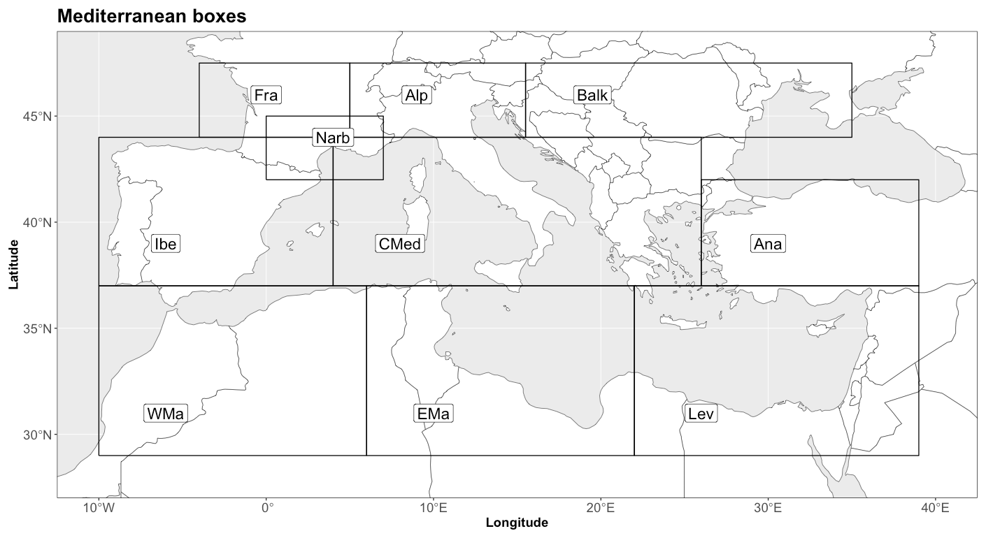
Figure 4Map of the 10 boxes defined in the Mediterranean region.
We also considered two other scenarios based on boundary conditions of +5 ∘C except for volcanic and solar activity. The idea is to assess whether volcanic and solar conditions typical of the Little Ice Age can moderate the effect of the strong increase in GHG concentrations. The first additional scenario (labeled +5 CV+) was assigned very substantial volcanic activity (0.8), the highest value in the last millennium, and low solar activity (i.e., 100). In contrast, the second additional scenario (labeled +5 CV−) was assigned low volcanic activity (0.1) and high solar activity (700), corresponding to those of the MCA. The forcing values are listed in Table 2.
2.5 Downscaling (step 1)
ESM resolution is too coarse (>100 km depending on the model) to assess the impact and risk of climate changes on ecosystems or human systems. Different approaches can be used to derive higher-resolution information. We use a statistical downscaling (SD) based on statistical relationships that link large-scale atmospheric variables with local and regional climate variables and that are applied to coarser-resolution model simulations (Su et al., 2016; Grouillet et al., 2016; Levavasseur et al., 2011), thereby providing higher-resolution estimates of climate variables. SD methods are among the less computationally expensive downscaling techniques.
The SD that we use assumes the hypothesis that the fields of climate anomalies do not depend on the grid resolution. So, they can be interpolated at a finer resolution than the initial resolution. We use a common 0.5∘ high-resolution (HR) grid for each climate simulation. It is provided by the high-resolution dataset of surface climate over global land areas (New et al., 2002) (which has a 10 min resolution and was aggregated at a 30 min resolution). This climatology is based on the 1961–1990 period. Each low-resolution (LR) anomaly field provided by the ESM is downscaled to the HR grid by the bilinear interpolator of platform R (function interp. surface of package fields). This HR anomaly field is added to the 1961–1990 climatological HR field of New et al. (2002). As the simulations are corrected by the differences between control simulations and observations, the main systematic biases of the model are removed. For the PMIP3 simulations (LGM, MidHol, and historical), the control is the preindustrial simulation (PI), so we use the 1900–1931 climatology very close to the PI (1861–1890) used by the recent IPCC reports (Allen et al., 2018). Figure 3 presents the global mean temperature for each period and scenario considered.
2.6 Vegetation modeling (BIOME4, step 2)
The ecosystem model is coupled offline to downscaled climate outputs and provides indications of land vegetation structure and productivity. Here, we used a process-based equilibrium vegetation model, BIOME4 (Kaplan et al., 2002), which has been successfully applied to similar questions before (Guiot and Cramer, 2016). While a wide range of climate simulations are necessary to ensure robust calibration, the use of a single ecosystem model is required to ensure that the same ecosystem variables are calculated for all simulations.
BIOME4 simulates some of the most important processes related to vegetation at the scale of the ecosystem, specifically photosynthesis, respiration, and evapotranspiration. It predicts structure and productivity of broad-scale land ecosystems from monthly temperature and rainfall values as well as annual CO2 concentration. It uses a photosynthesis scheme that simulates acclimation of plants to changed atmospheric CO2 by optimization of nitrogen allocation to foliage and by accounting for the effects of CO2 on net assimilation, stomatal conductance, leaf area index (LAI), and ecosystem water balance. BIOME4 is based on a sufficiently simple description of ecophysiological processes to allow broad-scale application. It represents substantial advantages over niche models because it has not been tuned to reproduce present-day potential vegetation, but rather to correctly simulate the main processes underlying the potential vegetation distribution, which are assumed to have been similar throughout the Holocene. BIOME4 does not account for human land use.
The inputs of the model are monthly average values of temperature, precipitation and sunshine percentage, atmospheric CO2 concentration, and soil texture. The temperature and precipitation variables are directly obtained from the simulations downscaled at the 0.5∘ grid. The sunshine percentages are obtained by linear regression on temperature and precipitation (Guiot et al., 2000). The absolute minimum temperature is derived from the mean temperature of the coldest month according to the quadratic equation of Prentice et al. (1992). The soil data are provided by the FAO (Zobler, 1986). The CO2 atmospheric concentration values are those used by CMIP5 and PMIP3 as boundary conditions for their simulations.
The outputs include net primary production (NPP) of each of the potentially occurring 13 plant functional types (PFTs), the total NPP, and the corresponding “biome type” from a set of 28 broad categories (Table 1). The model also provides several bioclimatic variables (Table 1).
2.7 The calibration of the emulator (step 3)
The numerous model outputs available in the CMIP and PMIP databases (Table 2) are used to calibrate robust statistical approximations of coupled ESMs and BIOME4, called the emulator (Kennedy and O'Hagan, 2000). Various emulators are used in climate science (Tran et al., 2016; Zhu et al., 2015; Rougier and Goldstein, 2014; Castruccio et al., 2014), including in paleoclimatology (Strassmann and Joos, 2018; Joos et al., 1996; Bounceur et al., 2015). Our approach is the first ESM-independent emulator because it is calibrated using a large set of model simulations under very different scenarios. The calibration is based on a geographically weighted regression (Brunsdon et al., 1998), whereby the ecosystem variables are expressed as functions of the global forcing variables.
For any choice of input q vector x (forcings), the climate simulator is , …, ym(x,s)), where m is the number of (bio)climatic variables whose response is to be analyzed and s is the location where the climate variables must be estimated. There are deterministic and possibly nonlinear functions. This model is a statistical representation of the ESM + BIOME4 model, with the very interesting properties to run very fast and provide an uncertainty description for the whole plausible input space (i.e., conform to physics, internally consistent and reasonable; Amara, 1991):
where s indicates the grid point out of a total of n points, yj(x,s) is the anomaly of the climatic variable j (out of m) at location s, i.e., the climate variable at time t minus the climate variable at time 0 (present), X is a matrix with v specified columns of the input global forcings (they do not depend on the location s), and e(s) is a stationary Gaussian variable . This can be considered a least-square problem wherein the coefficients βj(s) are estimated to minimize the sum of the squared errors. These coefficients can be written as
with W(s) as a matrix of weights specific to location s such that observations nearer to s are given greater weight than observations further away, and T is the transpose symbol. The estimation of βj(s) in location s is provided by weighting all the observations according to their distance from s, dis. The method is called geographically weighted regression (GWR) (Brunsdon et al., 1998). We use a bi-square weighting function so that W(s) is the diagonal matrix with elements
Here, h is called the bandwidth. We use the function gwr.basic of the package gw.model on R (Lu et al., 2014). We have chosen h=8 (in longitude and latitude degree units).
The emulator is trained on an ensemble of simulations performed on data sufficiently browsing the plausible input space. The more the input space is filled, the more robust the emulator will be. The fact that we have extended the range of forcing parameters to past, present, and future scenarios is an excellent way to fill this input space. Even if they are not a fully exhaustive sampling, it is reasonable to assume that they represent a model population (Chandler, 2013). The emulator is used to estimate the conditional probability distribution of the ecosystem variables (Table 1) in each location or biome based on the forcing variables (Table 4).
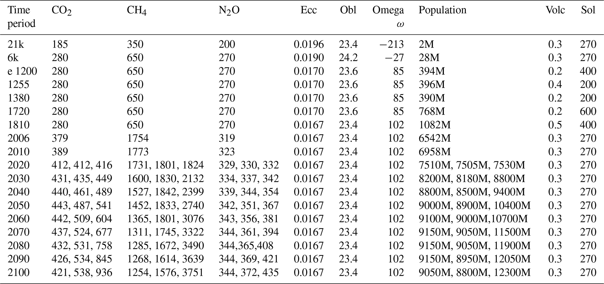
Table 4The nine global forcing variables and their values for the different periods considered. The global forcing variables are the predictors of the emulator; we give their values for the time slices used in the calibration: GHG atmospheric concentration (carbon dioxide, methane, nitrogen protoxide) in parts per million (ppm), Earth orbit parameters (eccentricity Ecc, obliquity Obl, omega ω), population in millions of people (M), volcanic activity (Volc), and solar activity (Sol, in MeV). Every column is one out of the v forcings of Eq. (1) (columns of X). For columns CO2, CH4, N2O, and population, we use observations until 2010 (see Sect. 2.1) and the values used by the three scenarios (RCP2.6, RCP4.5, RCP8.5) for projections (2020 to 2100).
The total number of simulations available for 18 time slices and three scenarios (for the 2020 to 2100 time slices) from 2 to 18 models is 582. As each one simulates climate for 65 559 grid points of the globe (after downscaling), the total number of available observations is . Because of their strong spatial correlation, it is not necessary to use all the grid points. To have a balance between the different biomes represented on the Earth, for each time slice and each model, we randomly draw a subset of grid points in each biome proportional to its representativity (the proportion of grid points with that biome). So, the calibration is done on about 3×10⁵ observations (the number is slightly lower than expected because some biomes are absent in some simulations).
As the global forcing variables have the same value for all the grid points for a given time slice and scenario, this may produce problems for the computation of the emulator; we have then added to them a small noise value (a Gaussian value with mean 0 and standard deviation equal to the initial standard deviation divided by 100).
Because of collinearity between the predictors (the global forcing variables), their dimensionality is reduced using principal components (PCs) of the normalized variables. The nine variables are reduced into five PCs together explaining 89 % of their total variance. The first PC is mainly related to the greenhouse gases and the global population, which is strongly correlated with them. PC3 shows the opposition between solar and volcanic activity. The other ones are difficult to interpret.
The 13 PFTs are aggregated into eight PFTs, representing the main types of vegetation across the world (Table 5). This enables reducing the dimension of the ecosystem variable vector. The number of variables to be estimated by the emulator is finally reduced to 17 (predictands in Table 6).
Table 5Aggregation of the plant functional types (PFTs). The 13 original PFTs are defined in Table 1.
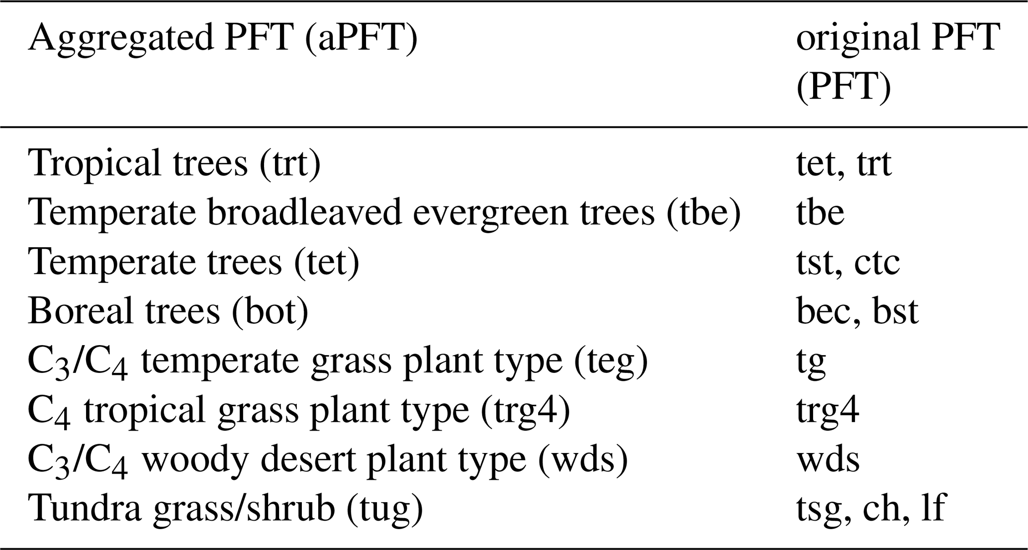
Table 6The t values of the linear regression between the PFT and bioclimatic variables as well as the five PCs of the forcing variables with the R2 (in %) of the linear model and the GWR model. For the latter, the coefficients cannot be displayed in a table and are represented as maps in Fig. 5.
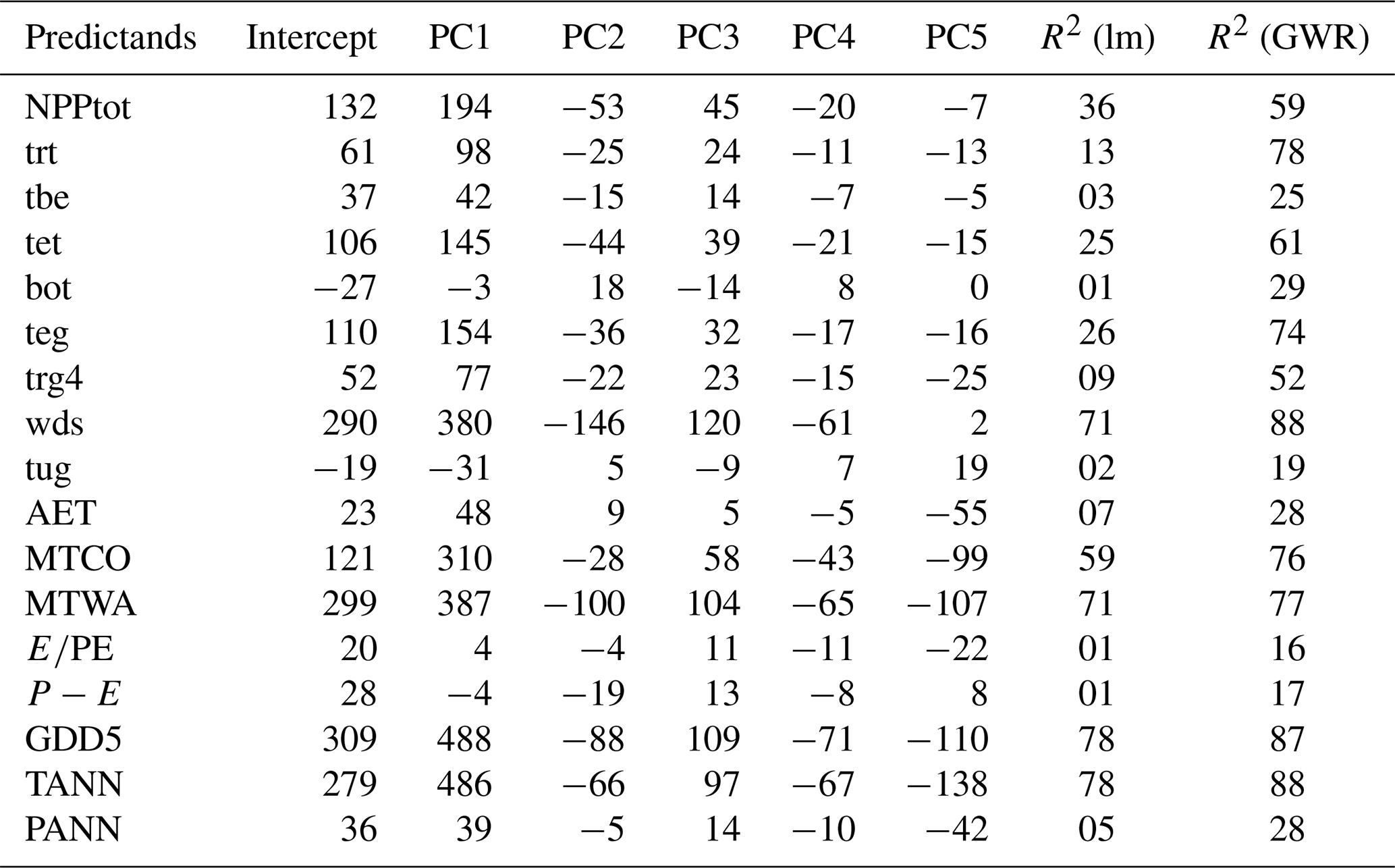
For comparison, we first apply a simple linear model to the data. Table 6 shows that most of the bioclimatic variables are not well-fitted. Indeed, only 9 of 17 have a proportion of reconstructed variance higher than 10 % (column R2 (lm)), which clearly shows that a single linear model is not adapted to our objective. The GWR model is much better as half of the bioclimatic variables have R2 higher than 0.50, but at the cost of a much larger effective number of parameters (ENPs) (ENP ∼ 1311 vs. 6 for the global linear model). As we have a very high number of observations (), the GWRs remain very significant. This is illustrated in Fig. 5 by the maps of the spatial distribution of the regression coefficients (they are standardized by their standard error, which comes to the t value). The degree of smoothing is defined by the bandwidth h (here set to 8). With a lower h, the patterns should be much patchier and the ENPs should become much larger, thereby diminishing the prediction capability of the model.
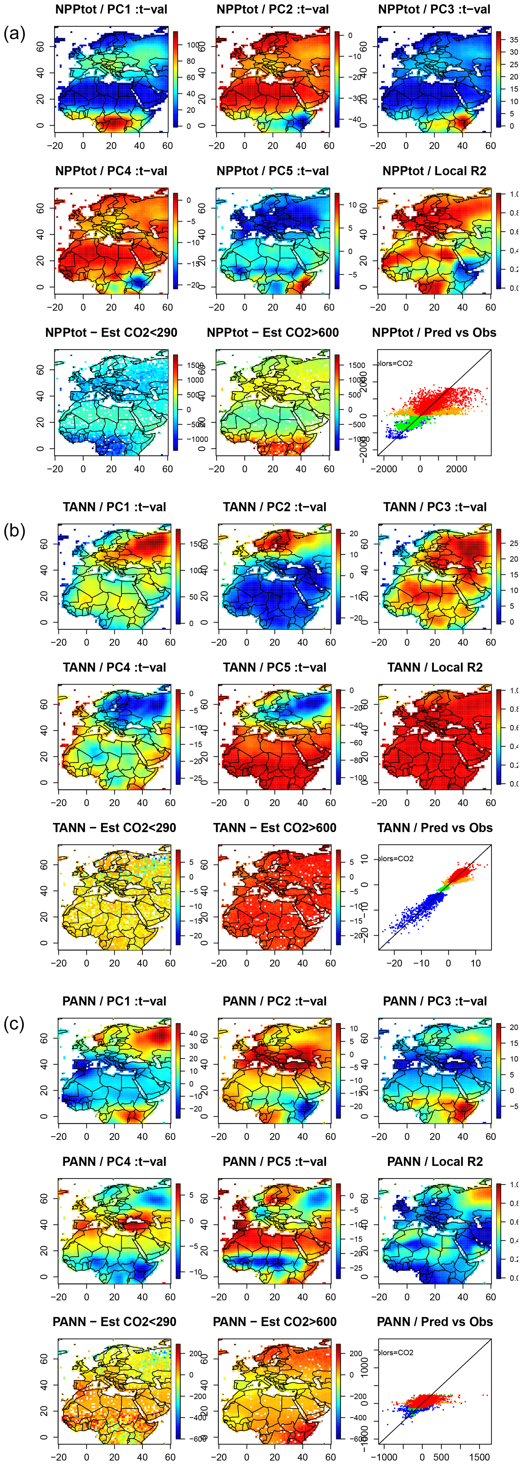
Figure 5Local (longitude × latitude) response of a few (bio)climatic variables to the PCs of forcing variables. The colors represent the t values (t-val) of the response (regression coefficient standard error). Maps 1 to 5 represent the first five PCs. Map 6 represents the R2 of the GWRs. Maps 7 and 8 represent the estimates for low-CO2 time slices (<290 ppm, i.e., LGM and mid-Holocene) and high-CO2 time slices (>600 ppm, second half of 21st century with scenario RCP8.5), respectively. The last graphic represents the estimates as a function of the observations: blue dots are for observations with CO2 < 250 ppm, green dots for CO2 belonging to [250, 400] ppm, orange dots for [400, 600] ppm, and red dots for CO2 > 600 ppm. The first series of maps is for the net primary production of the ecosystem (NPPtot); the second is for annual temperature (Tann), and the last one is for annual precipitation (Pann).
The interpretation is not straightforward because the predictors are not the forcing parameters but their PCs. Nevertheless, a partial interpretation is possible by using the correlation of the PCs with the forcings. For example, PC1 is correlated with the greenhouse gases (GHGs) and the population size, and Fig. 5 (Tann/PC1) shows that the maximum impact of the GHGs on temperature is in Russia. Figure 5 (Pann/PC1) shows that the GHGs have a negative effect on the precipitation around the Mediterranean and northern Africa and a positive effect on Russia. The decrease in precipitation according to the increase in GHGs is a well-known feature in the Mediterranean (Giorgi and Lionello, 2008). Figure 5 also shows that the annual temperature (Tann/Pred vs. Obs) is well-emulated with a strong correlation with CO2. It is also true, but to a lesser extent, for NPPtot. The annual precipitation estimates have a much lower variance than the observations.
2.8 Paleodata assimilation (step 4)
The climatic data estimated by the emulator have biases and uncertainties likely larger than those of the ESMs which have generated the calibration data. The first source of errors of the emulator is the same as the source of errors of the ESMs, which are imperfect representations of the real world. The second source of errors comes from the oversimplification, which consists of replacing a complex model by a statistical model, in considering that a few global forcings are able to generate the complex observed climate field. It is partly compensated for by the fact that the emulator is based on a large diversity of model simulations, in contrast to a single ESM. The third source of errors is the variance of the error terms ej(s) of Eq. (1): the statistical model does not perfectly fit the data. This prompted us to converge the emulator estimates to the real world represented by the paleoclimate data. This is known as paleodata assimilation (Goosse et al., 2012). This led to adjusting a few parameters known to have a large uncertainty to optimize temperature and precipitation using information given by proxies (Table 7).
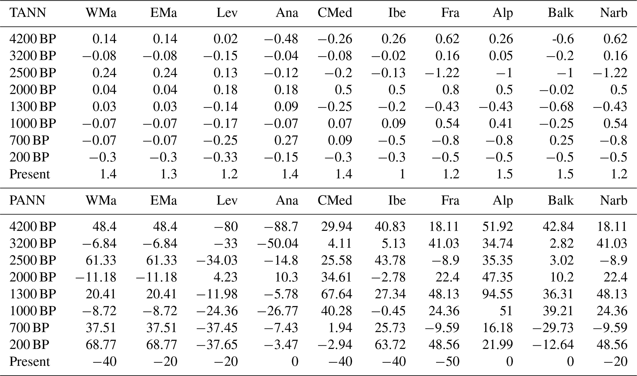
Table 7Proxy-based reconstruction of annual temperature (TANN, ∘C) and annual precipitation (PANN, mm). The values are expressed as anomalies from the preindustrial period for the 10 spatial boxes and the nine time slices, obtained from pollen (Guiot and Kaniewski, 2015) and corrected or made precise as indicated in Table 3.
These uncertain parameters are (i) local impact of volcanic activity, (ii) local impact of solar activity, (iii) a possible global bias for the temperature simulation (δT) and (iv) for the precipitation simulation (δP), and (v) the standard error of temperature (σT) and (vi) of precipitation (σP). Parameters (iii) and (iv) are related to a possible global ESM bias and are then independent of the geographical position. Parameters (v) and (vi) express the mean quadratic difference between observations and simulations and then contain the ESM mean error and the emulator mean error (after removing the effects of biases δT or δP).
The reconstructed annual temperature and precipitation values are expressed as anomalies relative to the present day for each time slice and each box given in Table 7. It shows that the first two time slices (4200 and 3200 yr BP) were characterized by dry conditions in the eastern Mediterranean Basin (boxes Lev, Ana). All the other time slices are characterized by temperature changes.
The statistical simplification of the emulator makes it possible to run it thousands of times in a relatively short computational time as required by the assimilation methods (Widmann et al., 2010). We use a Bayesian approach called the Markov chain Monte Carlo (MCMC) method, which makes it possible to converge towards the best parameters in the sense of probability distribution (Hargreaves and Annan, 2002).
Starting from the prior probability distributions of the six parameters, available climate reconstructions and model outputs provide estimates of their posterior probability distributions. For each time period, these six parameters were optimized to provide the best posterior probability distribution of mean temperature and precipitation at the centers of the 10 Mediterranean boxes. The prior probability distributions are given by uniform distributions delimited by the ±d (Table 8) for the volcanic and solar activity. The prior distribution of the other parameters was assumed to be uniform within wide ranges so that they were considered noninformative for the purpose of this study.
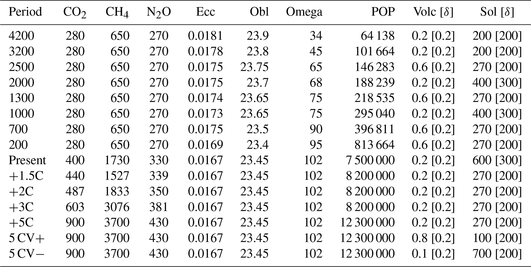
Table 8Forcing variables used for the 15 time slices and scenarios. The forcing greenhouse gas atmospheric concentrations (CO2, CH4, N2O), orbital parameters (ecc: eccentricity, Obl: obliquity, ω), population size (POP) in number of people, volcanic activity with uncertainty (d), and solar activity with uncertainty (d).
From Tables 3 and 7, we consider the 4200 and 3200 yr BP time slices to provide robust paleoclimatic information for precipitation and the other periods to provide robust information for temperature. Both the precipitation and temperature signals were robust for the present time slice. Even if we ultimately calculate both temperature and precipitation, only the robust variable(s) is (are) used to constrain the emulator.
2.9 The viticulture index (VI)
We subsequently applied our emulator to the question of how viticulture has evolved in the Mediterranean region and in response to which climatic stimuli and global forcing. Numerous bioclimate indices have been published to delimit viticultural zones in the world (Tonietto and Carbonneau, 2004; Santos et al., 2012; Howell, 2001). Among them, the following are cited: (1) the sum of degree days above 10 ∘C during the growing season or the heliothermal index of Huglin (HI), (2) the number of days with a minimum temperature below −17 ∘C, which is very important for the grapes growing in continental climates, (3) the minimum temperature of September (cool night index) important for the ripening, (4) the sum of the growing season of the monthly temperature multiplied by monthly precipitation (Hyl), and (5) the drought stress index (DI) related to the potential water balance of the soil during the growing season. Malheiro et al. (2010) proposed a composite index (CompI) calculated based on the ratio of years simultaneously satisfying four criteria (HI > 1400 degree days), DI > −100 mm, Hyl < 5100 ∘C mm−1, and Tmin > −17 ∘C).
Some of the climate variables needed for these indices were not available from the BIOME4 outputs. However, other variables, such as those associated with the net primary production of plant types, are very interesting because they include the CO2 effect on photosynthesis and water use efficiency. Considering only rain-fed viticulture, we propose the following index, VI:
where each of these factors denoted Ix follows the function
For x=NPPtrop, the net primary production of tropical plants, the interval [xmin, xmax] is [0, 10 kg C m−2]. For x=NPP, the total ecosystem net primary production, it is [500, 1000 kg C m−2]. For x=Pann, the total annual precipitation, it is [400, 800 mm]. For x=MTWA, the mean temperature of the warmest month, it is [18, 23 ∘C]. For x=MTCO, the mean temperature of the coldest month, it is [3, 12 ∘C]. The lower limit of 3 ∘C corresponds to a minimum mean monthly temperature with no chance of having an absolute daily minimum below −17 ∘C. For x=α, the actual to potential evapotranspiration ratio, it is [30 %, 60 %].
All factors except those related to NPPtrop assume that vine growth is limited only by the lower values and not by the higher values. Because there is no possible viticulture in the tropics (where temperature is not cold enough for an appropriate dormancy), is limited by its upper value.
This approach is a static approach as it is based on an equilibrium vegetation model only based on the mean state of the climate. The variability of the climate and therefore the extreme values of some variables are not considered. We are aware of these limitations, and it is the reason why our interpretations will only concern the potential extension of viticulture. Other weaknesses of the approach are the impossibility to consider the diversity of cultivars, the adaptation of grapes to frost, and the risk of biotic damage to the grapevines. This is a niche model approach of the same nature as those used in the literature cited at the beginning of this section. This oversimplified approach nevertheless has the advantage of providing a framework for the past and future trends and of being easily applicable to the past for which the data are rather limited.
3.1 Paleodata assimilation
From the posterior distributions (Table 9), it appears that the simulated volcanic activity impacts were the strongest during the cold periods (2500, 1300, 700, and 200 yr BP) and rather weak during the dry periods (4200 and 3200 yr BP) and warm periods (2000 and 1000 yr BP). The confidence intervals are significant as they do not overlap. For the present, volcanic and solar activities have no significant impact, which is easily explained by the dominant GHG effect (not used for constraining the assimilation). The impact of solar activity is not clear, as there is no significant difference between cold and warm periods or between the dry and wet periods. The temperature bias (δT independent of the spatial variability) is estimated to be between 0.6 and 1.6 ∘C for the periods between 2500 and 200 yr BP and is not significantly different from zero for the dry periods and for the present. The δP estimates were not significant for any time period. Figure 6 presents the overall correlations between the emulator outputs and the proxy-based reconstructions. A good emulation should be indicated by good coherency of both blue and black lines and a low variance of the dots around the black line. So, the temperature was particularly well-simulated by the emulator with a squared correlation (R2) of 0.76, but with an overestimation of the low temperatures. As expected, precipitation is less well-simulated with a significant R2 of 0.22 with an underestimation of the large (negative or positive) anomalies.
Table 9Posterior distribution of the parameters. The estimates are given by the best fit, and the CI is the 90 % confidence interval calculated on the 10 % best fits. Volc index has no units; the solar index is in megaelectron volts (MeV), T is in degrees Celsius (∘C), and P is in millimeters per year (mm yr−1).
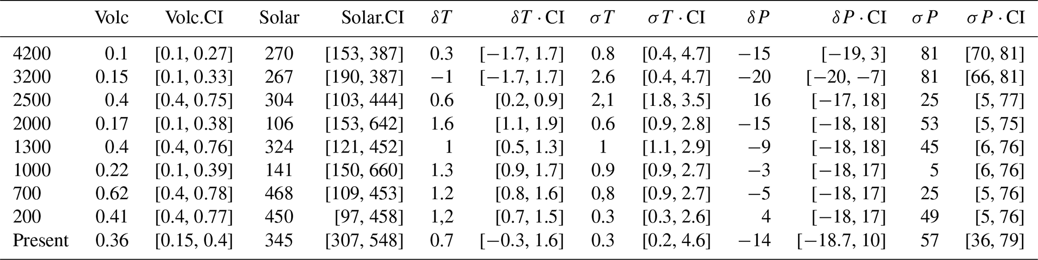
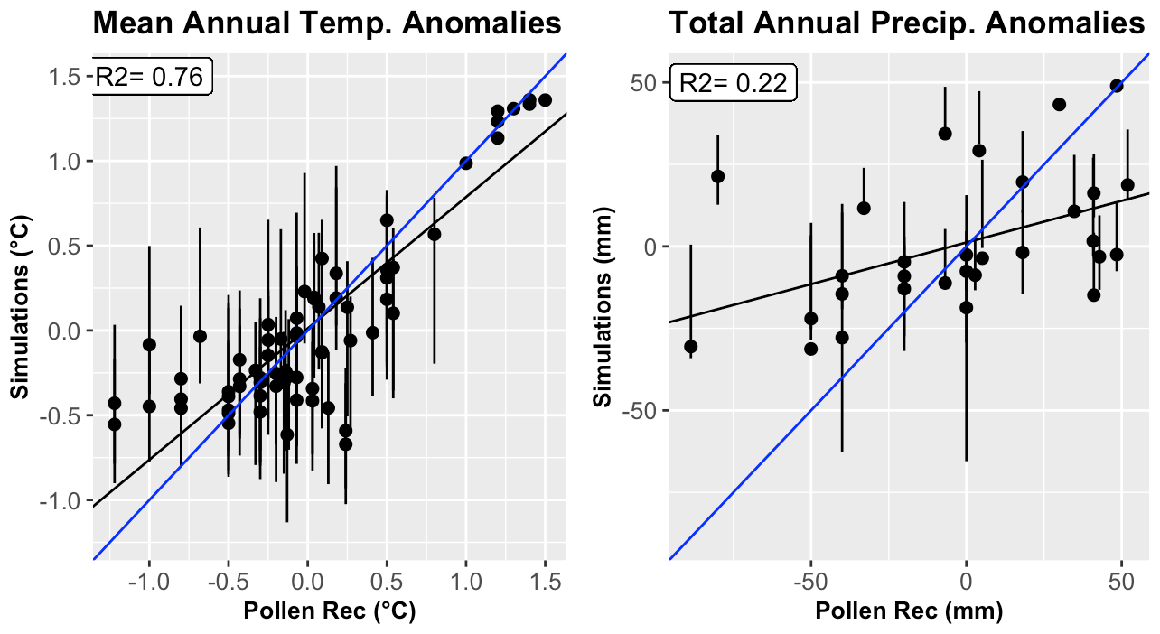
Figure 6Temperature and precipitation anomalies for the 10 Mediterranean boxes estimated by data assimilation versus data reconstructed from proxies. Temperature dots represent the mean annual temperature in the 10 boxes for the 11 periods from 2500 yr BP until the present, and precipitation dots represent the total annual precipitation in the two oldest periods (4200 and 3200 yr BP) and in the present. The vertical bars are the 90 % confidence intervals (CIs). The blue line is the perfect estimate line (R=1), and the black line is the regression line between the simulations and proxy reconstructions.
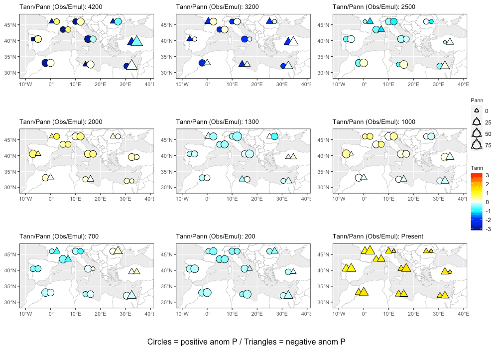
Figure 7Spatial distribution of the temperature and precipitation anomalies for the past and present time slices. The pairs of symbols are simulations (left symbols) and observations or pollen reconstructions (right symbols). The colors are used for the temperature anomalies. Triangles are used for negative precipitation anomalies and circles for the positive precipitation anomalies. The size of the triangles and circles is proportional to the absolute value of the precipitation anomalies.
3.2 Application of the emulator to past and future scenarios
This assimilation process was applied to simulate the annual temperature and precipitation for the 10 boxes and the 13 time slices and scenarios. The spatial patterns of the reconstructions and simulations are consistent, except for the temperatures at 4200 and 3200 yr BP. (Fig. 7). Therefore, global forcing variables can drive not only the mean climate evolution but also the spatial patterns reconstructed by the proxy data in the Mediterranean. Volcanic activity seems to be the main driver for the cold periods of the Iron Age (2500 yr BP), the LALIA (1300 yr BP), the LIA (700, 200 yr BP), and the warm periods of the RCO (2000 yr BP) and MCA (1000 yr BP). The main driver of the present warming and drying (present time in Fig. 7) is GHG forcing. For the 4200 and 3200 yr BP periods, the volcanic and solar activity drivers do not seem to be plausible explanations for the droughts, at least according to our emulator, and likely the ESMs; this also explains the absence of agreement.
Future projections (Fig. 8) show general warming for the four scenarios (+1.5C, +2C, +3C, +5C) that is particularly strong for +3C and +5C scenarios. The local warming is less strong in the areas influenced by the Atlantic Ocean (France and the Iberian Peninsula). For precipitation, the signal is weak for +1.5C and +2C with drier and wetter zones and clearer for +3C and +5C (all the symbols are triangles, i.e., negative). Combined with the warming, it is undeniable that water stress will increase considerably with +3C and +5C scenarios.
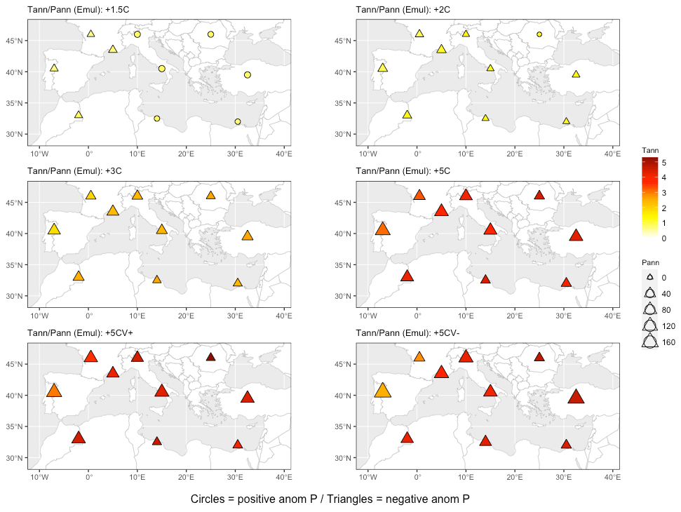
Figure 8Spatial distribution of the temperature and precipitation anomalies simulated for future time slices (scenarios). The colors are used for the temperature anomalies. Triangles are used for negative precipitation anomalies and circles for positive precipitation anomalies. The size of the triangles and circles is proportional to the absolute value of the precipitation anomalies.
To answer the question of whether volcanic activity can mitigate the impact of high GHG emissions, Fig. 8 shows that the temperature distributions of +5 CV+ and 5 CV− are quite similar, meaning that the cooling effect of volcanoes is relatively low in a large GHG emission scenario. The precipitation distributions of +5 CV+ and 5 CV− are similar in the western Mediterranean, and +5 CV+ produced slightly higher precipitation anomalies than +5 CV− in the eastern Mediterranean.
3.3 Independent validation
Additional independent validation was completed through comparisons with a tree-ring-based reconstruction of the Palmer Drought Severity Index (PDSI) (Cook et al., 2015) for the last 2 millennia, for which tree-ring data are available. The PDSI reflects the spring–summer soil moisture conditions. We compared this variable with the reconstruction of the (ratio of actual to potential evapotranspiration in %) variable provided by BIOME4. is a moisture index which is equal to zero when the soil is fully dry and 100 when it is fully wet. The range of the PDSI is usually between −6 and 6 units. Negative values correspond to conditions drier than normal. Considering that both indices are not fully similar, a visual comparison shows pretty good agreement (Fig. 9). So for 2000 BP, Iberia and central Europe were wet in both maps, and no PDSI data were available for the southern and eastern Mediterranean. For 1300 BP, all of Europe was dry in both maps except eastern Spain, which was as wet as at 2000 BP. For 1000 BP, the area surrounding the sea was wet except Greece in both maps, and for 700 BP all areas were wetter than 1000 BP in both maps.
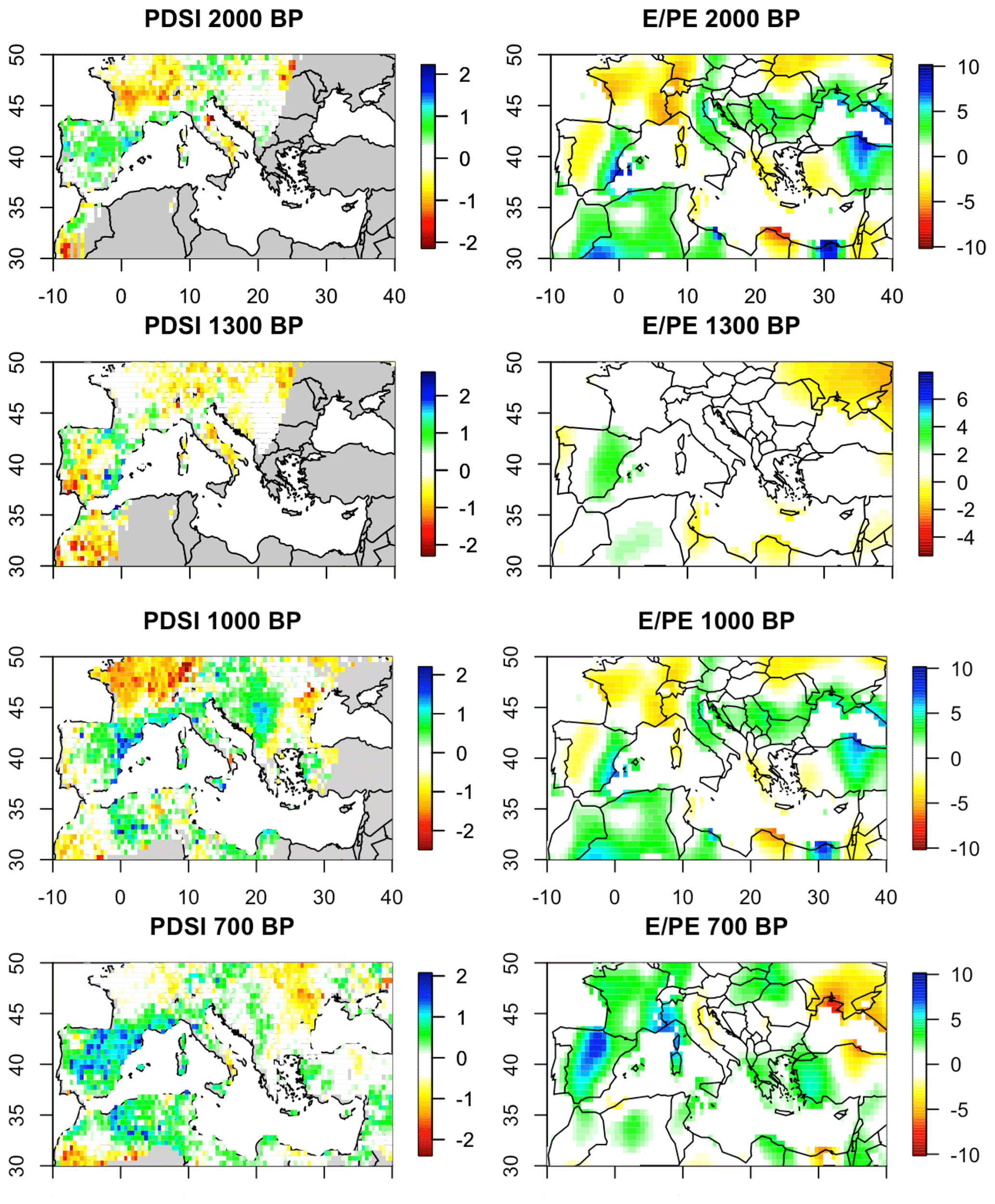
Figure 9Comparison of reconstructed in this paper with independently reconstructed Palmer Drought Severity Index (PDSI). The PDSI anomalies are based on the 1928–1978 reference period and are reconstructed from tree rings (Cook et al., 2015). is the ratio of actual to potential evapotranspiration obtained from the emulator (in %).
3.4 Evolution of viticulture from the Bronze Age to the end of the 21st century
Applied to the mean climate of 1980–2009, the viticulture index (VI) approximately reproduces the area in Europe where viticulture is present (Fraga et al., 2013) (Fig.10). As shown in Fig. 10a, the simulations give approximately the same limits, with some noticeable exceptions in Germany as well as the Alpine and Balkan regions, which are likely too continental to pass the MTCO criterion. This is the main limitation of our analysis. The presence of viticulture greatly depends on local factors such as valleys, slopes, and soil, which are not accounted for in our analysis. More generally, these discrepancies show that our index is not calibrated for continental regions with winters colder than 3 ∘C (on average). This threshold of 3 ∘C is likely overestimated by about 5 ∘C. So, we consider this index to adequately represent the macroclimate of potential vine distribution in western Europe and the Mediterranean region.
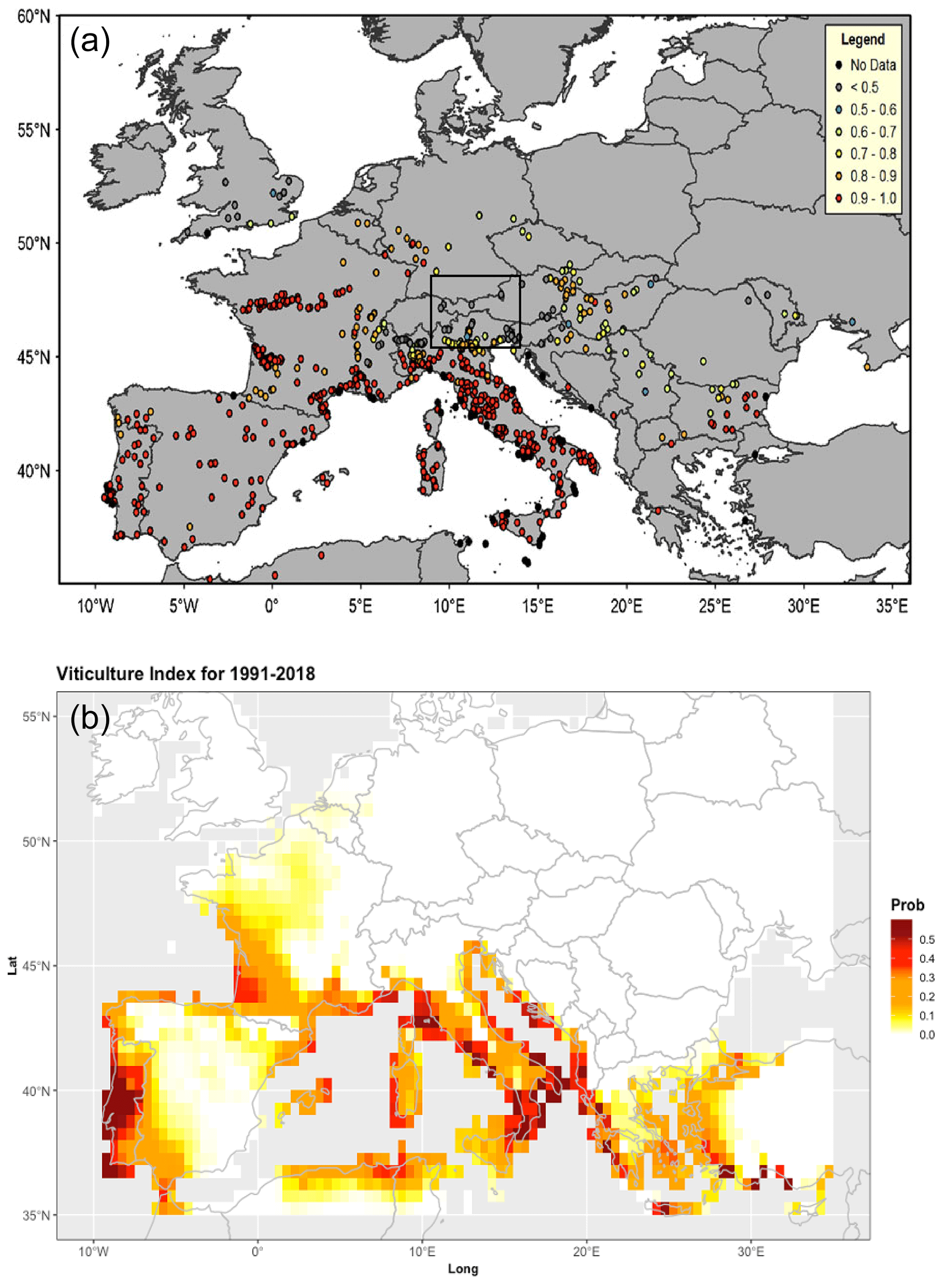
Figure 10Distribution of the wine sites: (a) European wine regions (circles) with the corresponding CompI value for the period of 1980–2009: from Fig. 1e of Fraga et al. (2013). (b) Simulation using the viticulture index calculated using 1961–1990 climate data.
The variables needed for viticulture in Eq. (4) are provided by the emulator for all time slices studied in the past time slices and for future scenarios. The procedure is sketched in Fig. 11. We modified the global forcings according to the values of Table 3 for the past and Table 2 for the future, and we thereby simulated, by applying the emulator, viticulture extension maps (Fig. 12). Figure 12 shows that during the dry time slices of 4200 and 3200 yr BP, the suitable areas were located between 34 and 46∘ N latitudes. During the cold periods (2500, 1300, 700, and 200 yr BP), they occupied approximately the same area between 34 and 47∘ N. During the warmer periods (2000 and 1000 yr BP), the southern limit did not change much, but the northern limit reached 49∘ N, implying that most of Gaul was suitable for viticulture, as already shown by Bernigaud et al. (2021). The present map is warmer than the preindustrial period (200 yr BP slice), which suggests that viticulture is now at its maximum potential extension in 4000 years, up to 51∘ N. Because of the drier conditions, the southern limit has shifted from 34 to 35∘ N. Note that these variations only depend on climate changes, without any consideration of other factors such as types of soils, which are very important for wine quality.
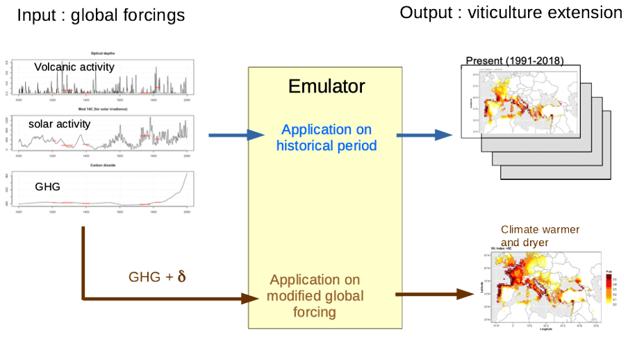
Figure 11Diagram of the application of the emulator to reconstruct and predict the viticulture extension.
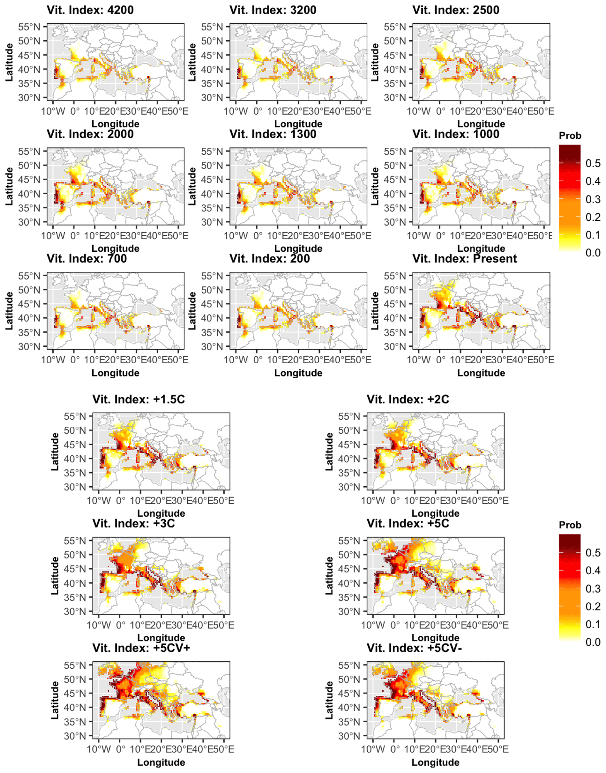
Figure 12Distribution of the viticulture index (Vit. Index) for several time slices of the past (in yr BP) and future scenarios (expressed as anomalies of global temperature vs. preindustrial reference). The index is labeled VI and is explained in Eq. (4). White areas indicate where it is impossible to cultivate vine.
In the future projections, the northern extension of potential viticulture should shift from 51∘ N (+1.5C scenario) to 53∘ N (+3C scenario) and even above 55∘ N (for the +5C scenario). This would allow viticulture to be possible up to central England, but it would regress in the south due to stronger water stress. In the Iberian Peninsula, only the Atlantic coast should be suitable for cultivating wine grapes unless there is significant irrigation. These projected unfavorable conditions were in agreement with Fraga et al. (2013) based on other viticulture indices. The 5 CV+ and 5 CV− scenarios appear quite like the 5C scenario, indicating that the effect of high or low volcanic activities should have a weak effect on the potential distribution of viticulture in comparison to a strong GHG forcing.
The results are summarized in Fig. 13. In the past, only the warm regions of the southern band (29–37∘ N) had a suitable wine-growing area equivalent to the present. The central geographical band (37–44∘ N) and the northern one (44–48∘ N) underwent sudden changes in the viticulture area, first from the cool Iron Age (2500 yr BP) to the RCO (2000 yr BP) and later from the end of the LIA (200 yr BP) to the present. The cold periods are all characterized by a decline in viticulture at latitudes above 37∘ N. For the future projections, northward displacements are likely to be drastic from +3 ∘C global warming. Viticulture potential will likely disappear from North Africa and is set to decrease drastically in the Iberian Peninsula. In contrast, potential productive areas will likely expand at latitudes above 50∘ N, in the Balkans, and in the Alps, which is a significant change considering that our approach underestimates the grapevine potential of continental climates.
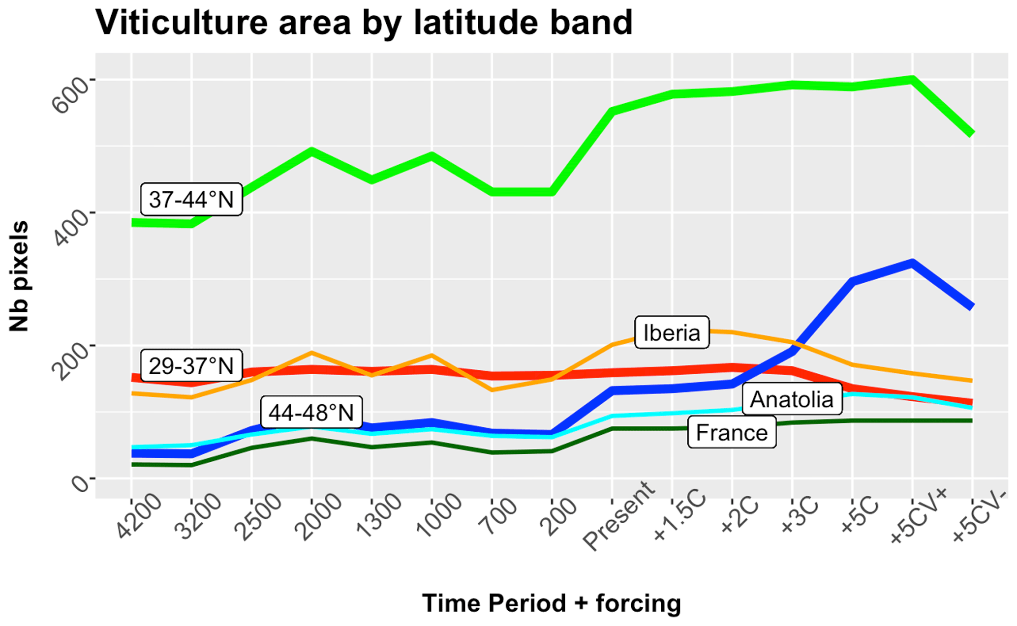
Figure 13Synthesis of the evolution of viticulture in the Mediterranean area. The curves represent three bands of latitude: the southern band with latitude < 37∘ N in red, the center band with latitudes between 37 and 44∘ N in green, and the northern band with latitudes between 44 and 48∘ N in blue). The thin lines show the results for the boxes corresponding to the Iberian Peninsula, Anatolia, and France (definition in Fig. 4). The scenarios and time slices are defined in Table 8. The x axis gives the center of the time slices considered or the future scenario.
For the two additional scenarios of high emissions combined with extreme volcanic and solar activities, the question is whether an entirely hypothetical set of strong volcanic events could slow down the decline in viticulture in the south. The answer is slightly positive for Spain, Italy, Greece, and Turkey (green curve increases for +5 CV+ and decreases for +5 CV−), but it is negative in North Africa and the Levant (red curve) because the water stress should remain too substantial. The effect is also positive in the northern band and Turkey (the blue and cyan curves increase for +5 CV+ and decrease for +5 CV−). In all the cases, the effect was clearly too small to compensate for the GHG effect.
The discussion considers six points, which concern methodological innovations as well as contributions to climate science and viticulture science.
-
We used an emulator approach which recently became popular in the ESM community. In some ways, it has also been used with paleoclimatic data (Crucifix, 2012; Joos et al., 1996),= and to emulate a climate–vegetation system (Foley et al., 2016). But this study is the first to use an ensemble of climate models, along with several forcing variables provided by past, present, and future states, to project vegetation conditions from global climate drivers. This has involved solving several technical issues.
-
We showed that the major climatic variations of the last millennia in the Mediterranean Basin can be attributed to volcanic activity, whereas the effects of solar activity were negligible. The effects of volcanic and solar activities have been largely debated, as the reconstruction of temperatures in the last millennium from tree rings has often shown less significant cooling than the model simulations (Mann et al., 2012). A more recent tree-based reconstruction (Stoffel et al., 2015) showed substantial summer cooling after the Samalas eruption in 1257 and that of Tambora in 1816, but less intense than simulated. Luterbacher et al. (2016) showed that solar activity had a relatively weak influence on the European summer temperatures. Thus, our results are in line with the state of the art in the scientific literature.
-
The effect of this volcanic forcing has a clear spatial pattern across the Mediterranean Basin. From 2500 yr BP to the present, temperature variations were more significant in the north and in the west than in the southeast (Fig. 7). Fischer et al. (2007) found that northern and western Europe were the coldest and driest areas after an eruption. They also found that southern Europe, North Africa, and the Levant have experienced milder and wetter weather than at present. Part of this pattern might be due to regional feedbacks of vegetation on the climate. Some climate model simulations have shown (Reale and Dirmeyer, 2000) that wetter vegetation during the RCO may have induced a northward shift of the Intertropical Convergence Zone during the summer over the African continent with an increase in moisture in North Africa and Iberia, as well as a decrease in the central Mediterranean (Reale and Shukla, 2000). In the future, the southeast should be relatively less dry and warmer than the northwest, especially in summer, which is consistent with our results (Fig. 8) (Giorgi and Lionello, 2008).
-
Our simulations of climate change effect on viticulture are mostly concerned with larger-scale regional production systems since they would require nearly full-time engagement of wine growers with high certainty of production every year, sufficient for speculative trade. For smaller domains and local consumption, it may have also been possible to produce wine under degraded or unstable weather conditions. For example, in England, viticulture continued to be practiced on land owned by the church, even as risks increased due to a wetter climate, with cooler summers and milder winters (Clout, 2013). In most wine regions in western Europe, particularly in France, the grape harvest dates were advanced after the LIA and particularly after the 1940s (Le Roy Ladurie et al., 2006). For example, from 1945 to the beginning of the 21st century, in Chateauneuf du Pape (southern Rhone Valley, France) the harvest date advanced on average from 1 October to 11 September (Ganichot, 2002). This change is related to summer warming, but factors related to wine quality, agricultural practices, and alcohol content regulation may induce a bias in the interpretation (de Cortázar-Atauri et al., 2010). In the Languedoc region, the potential alcohol content increased by two degrees from 1984 to 2013 (van Leeuwen and Darriet, 2016). Even if the alcohol content does not exactly reflect the grape yields, earlier harvest dates with a higher sugar content have clearly been related to improved conditions of grape cultivation since the LIA, which is also related to increased productivity. Another climate-sensitive symbol of Mediterranean agriculture is olive trees. Moriondo et al. (2013) found three characteristic periods in olive growing, namely the RCO (300 BCE to 400 CE) and the MCA (900 CE to 1200 CE), during which olive-growing areas expanded northward, and the LIA (1400 CE to 1900 CE) during which a contraction was reported. This is consistent with the variations in viticulture, at least in western Europe and the Mediterranean area as our VI is not properly calibrated for strongly continental climates.
-
Major difficulties are forecast for 21st century viticulture in Spain and North Africa. These are particularly important for global warming levels of +3 ∘C and more. Caffarra and Eccel (2011) showed that the projected warming should make some mountain sites at approximately 1000 m climatically suitable for viticulture before the end of this century. The MCA limit will certainly be passed. However, other factors could become limiting, such as excessively mild winters that enable pest attacks and infections, lack of expertise in vine growing and wine making, and products that are more expensive than the current Mediterranean wines (Clout, 2013). Other limitations are extreme events (late frost, flooding). More frequent and more intense heatwaves will no longer be favorable to viticulture at the present southern Mediterranean limit of its niche. These factors are not considered in our approach. A recent study considering grape varieties showed (Sgubin et al., 2022) that, for global temperature anomalies below 2 ∘C, the mean relative area loss was estimated to be 3.9 % ∘C−1, while for higher values of global warming this loss trend is estimated to be a much larger rate of 17.1 % ∘C−1. This confirms the existence of a safe limit below 2 ∘C of global warming for the European wine-making sector, above which adaptation might become far more challenging.
-
It is not very likely that intense volcanic activity could slow down this decline because (despite the many other negative consequences of such events) the beneficial climatic effects of this activity would be highest in regions with increased wine-growing potential under global warming (Turkey, northern Europe, the Alps, and the Balkans) and negligible in North Africa. IPCC has assessed the literature concerning the question of whether volcanic eruptions could be analogous for geoengineering proposals for climate mitigation (Myhre et al., 2013). Independent of their possible negative side effects, solar radiation modification (SRM), consisting of injecting sulfur aerosols in the stratosphere like a volcano does, is likely not an efficient technique to cool the atmosphere. Indeed, our results show that very strong volcanic activity, even accompanied by low solar activity, should not have any significant effects on viticulture extension in comparison to the radiative forcing from anthropogenic GHG emissions.
We demonstrated the efficiency of a statistical emulator based on multiple ESMs and calibrated over a large range of forcing and climate states to link the production of a regionally important crop (grapes) to global climate forcing variables. There are two main methodological innovations: (i) past climate simulations are used together with future ones to calibrate a robust emulator, and (ii) this emulator is independent of any single model because it captures what is common among all the available model simulations. But it remains an emulator which captures no more than the information contained in the ESMs.
Using it on past time slices, we showed that volcanic activity is a good predictor of the past temperature variations in the Mediterranean Basin and consequently of the viticulture productivity. During the warm phases of historical times (the Roman Climate Optimum and the Medieval Climate Anomaly) characterized by low volcanic activity, the viticulture area has shifted northward from 47 to 49∘ N. This historical limit has already been passed at the present time as it has already shifted to 51∘ N, and with global warming of +3 ∘C, it should pass the 53∘ N limit. Even if, in the warm periods of the past, North African and Iberian farmers never had real difficulties in cultivating grapes, they will meet large difficulties with global warming of +3 ∘C or more, except on the Atlantic margin. Moreover, our sensitivity experiments show that even intense volcanic activity is not sufficient to stop this decline.
All data, codes, and materials used in the analyses are available at https://github.com/douane7/C5P3_B4_emul.git (douane7, 2023).
JG designed the study, did the formal analyses, performed the visualisations, and wrote the draft of the paper. AB, NB, and LB participated in the conceptualisation of the study and reviewed and edited the paper. WC reviewed and edited the paper.
The contact author has declared that none of the authors has any competing interests.
Publisher's note: Copernicus Publications remains neutral with regard to jurisdictional claims in published maps and institutional affiliations.
Charles La Via edited the English in an earlier version of the paper.
This work has been funded by the Excellence Initiative of Aix-Marseille University A*MIDEX, a French “Investissements d'Avenir” program (project RDMED), and the Labex OT-Med project (project ANR-11-LABEX-0061).
This paper was edited by Martin Claussen and reviewed by two anonymous referees.
Allen, M. R., Dube, O. P., Solecki, W., Aragón-Durand, F., Cramer, W., Humphreys, S., Kainuma, M., Kala, J., Mahowald, N., Mulugetta, Y., Perez, R., Wairiu, M., and Zickfeld, K.: Framing and Context, in: Global Warming of 1.5 ∘C, in: An IPCC Special Report on the impacts of global warming of 1.5 ∘C above pre-industrial levels and related global greenhouse gas emission pathways, in the context of strengthening the global response to the threat of climate change, edited by: Masson-Delmotte, V., Zhai, P., Pörtner, H.-O., Roberts, D., Skea, J., Shukla, P. R., Pirani, A., Moufouma-Okia, W., Péan, C., Pidcock, R., Connors, S., Matthews, J. B. R., Chen, Y., Zhou, X., Gomis, M. I., Lonnoy, E., Maycock, T., Tignor, M., and Water, T., Cambridge University Press, Cambridge, UK and New York, NY, USA, 49–92, https://doi.org/10.1017/9781009157940.003, 2018.
Amara, R.: Views on futures research methodology, Futures, 23, 645–649, https://doi.org/10.1016/0016-3287(91)90085-G, 1991.
Berger, A. and Loutre, M. F.: Insolation values for the climate of the last 10,000,000 years, Quaternary Sci. Rev., 10, 297–317, 1991.
Bernigaud, N., Bondeau, A., and Guiot, J.: Understanding the development of viticulture in Roman Gaul during and after the Roman climate optimum: The contribution of spatial analysis and agro-ecosystem modeling, J. Archaeol. Sci. Rep., 38, 1–9, https://doi.org/10.1016/j.jasrep.2021.103099, 2021.
Bouby, L., Marinval, P., and Terral, J.-F.: From secondary to speculative ProductIon? the Protohistory history of viticulture in Southern France, in: Plants and People: choices and diversity through time, edited by: Chevalier, A., Marinova, E., and Chocarro, L. P., Oxbow Book, London, Philadelphia, 175–181, https://doi.org/10.2307/1309151, 2014.
Bouby, L., Wales, N., Jalabadze, M., Rusishvili, N., Bonhomme, V., Ramos-Madrigal, J., Evin, A., Ivorra, S., Lacombe, T., Pagnoux, C., Boaretto, E., Gilbert, M. T. P., Bacilieri, R., Lordkipanidze, D., and Maghradze, D.: Tracking the history of grape cultivation in Georgia combining geometric morphometrics and ancient DNA, Veg. Hist. Archaeobot., 30, 63–76, https://doi.org/10.1007/s00334-020-00803-0, 2021.
Bounceur, N., Crucifix, M., and Wilkinson, R. D.: Global sensitivity analysis of the climate-vegetation system to astronomical forcing: An emulator-based approach, Earth Syst. Dynam., 6, 205–224, https://doi.org/10.5194/esd-6-205-2015, 2015.
Braconnot, P., Harrison, S. P., Kageyama, M., Bartlein, P. J., Masson-Delmotte, V., Abe-Ouchi, A., Otto-Bliesner, B., and Zhao, Y.: Evaluation of climate models using palaeoclimatic data, Nat. Clim. Change, 2, 417–424, https://doi.org/10.1038/nclimate1456, 2012.
Brayshaw, D. J., Hoskins, B., and Black, E.: Some physical drivers of changes in the winter storm tracks over the North Atlantic and Mediterranean during the Holocene, Philos. T. Roy. Soc. A, 368, 5185–5223, https://doi.org/10.1098/rsta.2010.0180, 2010.
Brown, A. G., Meadows, I., Turner, S. D., and Mattingley, D.: Roman vineyards in Britain: stratigraphic and palynological data from Wollaston in the Nene Valley, England, Antiquity, 75, 745–757, 2001.
Brun, J.-P.: 15. Viticulture et oléiculture en Gaule, in: Comment les Gaules devinrent romaines, edited by: Ouzoulias, P., La Découverte, Paris, 231–253, 2010.
Brunsdon, C., Fotheringham, S., and Charlton, M.: Geographically weighted regression – Modelling spatial non-stationarity, J. Roy. Stat. Soc. Ser. D, 47, 431–443, https://doi.org/10.1111/1467-9884.00145, 1998.
Büntgen, U., Tegel, W., Nicolussi, K., McCormick, M., Frank, D., Trouet, V., Kaplan, J. O., Herzig, F., Heussner, K.-U., Wanner, H., Luterbacher, J., and Esper, J.: 2500 years of European climate variability and human susceptibility, Science, 331, 578–582, https://doi.org/10.1126/science.1197175, 2011.
Büntgen, U., Myglan, V. S., Ljungqvist, F. C., Mccormick, M., Di Cosmo, N., Sigl, M., Jungclaus, J., Wagner, S., Krusic, P. J., Esper, J., Kaplan, J. O., De Vaan, M. A. C., Luterbacher, J., Wacker, L., and Tegel, W.: Cooling and societal change during the Late Antique Little Ice Age from 536 to around 660 AD, Nat. Geosci., 9, 231–236, https://doi.org/10.1038/NGEO2652, 2016.
Caffarra, A. and Eccel, E.: Projecting the impacts of climate change on the phenology of grapevine in a mountain area, Aust. J. Grape Wine Res., 17, 52–61, https://doi.org/10.1111/j.1755-0238.2010.00118.x, 2011.
Castruccio, S., McInerney, D. J., Stein, M. L., Crouch, F. L., Jacob, R. L., and Moyer, E. J.: Statistical emulation of climate model projections based on precomputed GCM runs, J. Climate, 27, 1829–1844, https://doi.org/10.1175/JCLI-D-13-00099.1, 2014.
Chandler, R. E.: Exploiting strength, discounting weakness: Combining information from multiple climate simulators, Philos. T. Roy. Soc. A, 371, 20120388, https://doi.org/10.1098/rsta.2012.0388, 2013.
Clout, H.: An Overview of the Fluctuating Fortunes of Viticulture in England and Wales, EchoGeo, 23, https://doi.org/10.4000/echogeo.13333, 2013.
Cook, E. R., Seager, R., Kushnir, Y., Briffa, K. R., Büntgen, U., Frank, D., Krusic, P. J., Tegel, W., Schrier, G. Vander, Andreu-Hayles, L., Baillie, M., Baittinger, C., Bleicher, N., Bonde, N., Brown, D., Carrer, M., Cooper, R., Eùfar, K., DIttmar, C., Esper, J., Griggs, C., Gunnarson, B., Günther, B., Gutierrez, E., Haneca, K., Helama, S., Herzig, F., Heussner, K. U., Hofmann, J., Janda, P., Kontic, R., Köse, N., Kyncl, T., Levaniè, T., Linderholm, H., Manning, S., Melvin, T. M., Miles, D., Neuwirth, B., Nicolussi, K., Nola, P., Panayotov, M., Popa, I., Rothe, A., Seftigen, K., Seim, A., Svarva, H., Svoboda, M., Thun, T., Timonen, M., Touchan, R., Trotsiuk, V., Trouet, V., Walder, F., Wany, T., Wilson, R., and Zang, C.: Old World megadroughts and pluvials during the Common Era, Sci. Adv., 1, 37, https://doi.org/10.1126/sciadv.1500561, 2015.
Crowley, T. J. and Unterman, M. B.: Technical details concerning development of a 1200 yr proxy index for global volcanism, Earth Syst. Sci. Data, 5, 187–197, https://doi.org/10.5194/essd-5-187-2013, 2013.
Crucifix, M.: Traditional and novel approaches to palaeoclimate modelling, Quaternary Sci. Rev., 57, 1–16, https://doi.org/10.1016/j.quascirev.2012.09.010, 2012.
de Cortázar-Atauri, I. G., Daux, V., Garnier, E., Yiou, P., Viovy, N., Seguin, B., Boursiquot, J. M., Parker, A. K., va Leeuwen, C., and Chuine, I.: Climate reconstructions from grape harvest dates: Methodology and uncertainties, Holocene, 20, 599–608, https://doi.org/10.1177/0959683609356585, 2010.
douane7: C5P3_B4_emul, GitHub [code and data set], https://github.com/douane7/C5P3_B4_emul (last access: 16 June 2023), 2023.
Finné, M., Holmgren, K., Sundqvist, H. S., Weiberg, E., and Lindblom, M.: Climate in the eastern Mediterranean, and adjacent regions, during the past 6000 years – A review, J. Archaeol. Sci., 38, 3153–3173, https://doi.org/10.1016/j.jas.2011.05.007, 2011.
Fischer, E. a., Luterbacher, J., Zorita, E., Tett, S. F. B., Casty, C., and Wanner, H.: European climate response to tropical volcanic eruptions over the last half millennium, Geophys. Res. Lett., 34, 1–6, https://doi.org/10.1029/2006GL027992, 2007.
Foley, A. M., Holden, P. B., Edwards, N. R., Mercure, J.-F., Salas, P., Pollitt, H., and Chewpreecha, U.: Climate model emulation in an integrated assessment framework: a case study for mitigation policies in the electricity sector, Earth Syst. Dynam., 7, 119–132, https://doi.org/10.5194/esd-7-119-2016, 2016.
Fraga, H., Malheiro, A. C., Moutinho-Pereira, J., and Santos, J. A.: Future scenarios for viticultural zoning in Europe: Ensemble projections and uncertainties, Int. J. Biometeorol., 57, 909–925, https://doi.org/10.1007/s00484-012-0617-8, 2013.
Franklin, J., Serra-Diaz, J. M., Syphard, A. D., and Regan, H. M.: Global change and terrestrial plant community dynamics, P. Natl. Acad. Sci. USA, 113, 3725–3734, https://doi.org/10.1073/pnas.1519911113, 2016.
Frieler, K., Lange, S., Piontek, F., Reyer, C. P. O., Schewe, J., Warszawski, L., Zhao, F., Chini, L., Denvil, S., Emanuel, K., Geiger, T., Halladay, K., Hurtt, G., Mengel, M., Murakami, D., Ostberg, S., Popp, A., and Riva, R.: Assessing the impacts of 1.5 ∘C global warming – simulation protocol of the Inter-Sectoral Impact Model Intercomparison Project (ISIMIP2b), Geosci. Model Dev., 10, 4321–4345, https://doi.org/10.5194/gmd-10-4321-2017, 2017.
Fuks, D., Ackermann, O., Ayalon, A., Bar-Matthews, M., Bar-Oz, G., Levi, Y., Maeir, A. M., Weiss, E., Zilberman, T., and Safrai, Z.: Dust clouds, climate change and coins: consiliences of palaeoclimate and economy in the Late Antique southern Levant, Levant, 49, 205–223, https://doi.org/10.1080/00758914.2017.1379181, 2017.
Ganichot, B.: Évolution de la date des vendanges dans les Côtes du Rhône méridionales, in: Actes des 6e Rencontres rhodaniennes, Institut Rhodanien, Orange, France, 38–41, 2002.
Giorgi, F. and Lionello, P.: Climate change projections for the Mediterranean region, Global Planet. Change, 63, 90–104, https://doi.org/10.1016/j.gloplacha.2007.09.005, 2008.
Goosse, H., Guiot, J., Mann, M. E. M. E., Dubinkina, S., and Sallaz-Damaz, Y.: The medieval climate anomaly in Europe: Comparison of the summer and annual mean signals in two reconstructions and in simulations with data assimilation, Global Planet. Change, 84–85, 35–47, https://doi.org/10.1016/j.gloplacha.2011.07.002, 2012.
Grouillet, B., Ruelland, D., Ayar, P. V., and Vrac, M.: Sensitivity analysis of runoff modeling to statistical downscaling models in the western Mediterranean, Hydrol. Earth Syst. Sci., 20, 1031–1047, https://doi.org/10.5194/hess-20-1031-2016, 2016.
Guiot, J. and Cramer, W.: Climate change: The 2015 Paris Agreement thresholds and Mediterranean basin ecosystems, Science, 354, 4528–4532, https://doi.org/10.1126/science.aah5015, 2016.
Guiot, J. and Kaniewski, D.: The Mediterranean Basin and Southern Europe in a warmer world: What can we learn from the past?, Front. Earth Sci., 3, 28, https://doi.org/10.3389/feart.2015.00028, 2015.
Guiot, J., Torre, F., Jolly, D., Peyron, O., Boreux, J. J. J., Cheddadi, R., Borreux, J. J., and Cheddadi, R.: Inverse vegetation modeling by Monte Carlo sampling to reconstruct paleoclimate under changed precipitation seasonality and CO2 conditions: application to glacial climate in Mediterranean region, Ecol. Model., 127, 119–140, https://doi.org/10.1016/S0304-3800(99)00219-7, 2000.
Hargreaves, J. and Annan, J.: Assimilation of paleo-data in simple Earth system model, Clim. Dynam., 19, 371–381, https://doi.org/10.1007/s00382-002-0241-0, 2002.
Holzhauser, H., Magny, M., and Zumbuhl, H. J.: Glacier and lake-level variations in west-central Europe over the last 3500 years, Holocene, 15, 789–801, https://doi.org/10.1191/0959683605hl853ra, 2005.
Howell, S. G.: Sustainable Grape Productivity and the Growth-Yield Relationship, Am. J. Enol. Vitic., 52, 165–174, 2001.
Izdebski, A., Holmgren, K., Weiberg, E., Stocker, S. R., Buntgen, U., Florenzano, A., Gogou, A., Leroy, S. A. G., Luterbacher, J., Martrat, B., Masi, A., Mercuri, A. M., Montagna, P., Sadori, L., Schneider, A., Sicre, M. A., Triantaphyllou, M., and Xoplaki, E.: Realising consilience: How better communication between archaeologists, historians and natural scientists can transform the study of past climate change in the Mediterranean, Quaternary Sci. Rev., 136, 5–22, https://doi.org/10.1016/j.quascirev.2015.10.038, 2016.
Jones, P. D., Lister, D. H., Osborn, T. J., Harpham, C., Salmon, M., and Morice, C. P.: Hemispheric and large-scale land-surface air temperature variations: An extensive revision and an update to 2010, J. Geophys. Res.-Atmos., 117, D05127, https://doi.org/10.1029/2011JD017139, 2012.
Joos, F., Bruno, M., Fink, R., Siegenthaler, U., Stocker, T., LeQuere, C., and Sarmiento, J. L.: An efficient and accurate representation of complex oceanic and biospheric models of anthropogenic carbon uptake, Tellus B, 48, 397–417, 1996.
Kaniewski, D., Guiot, J., and Van Campo, E.: Drought and societal collapse 3200 years ago in the Eastern Mediterranean: A review, Wiley Interdisciplin. Rev. Clim. Change, 6, 369–382, https://doi.org/10.1002/wcc.345, 2015.
Kaniewski, D., Marriner, N., Cheddadi, R., Guiot, J., and Van Campo, E.: The 4.2 ka BP event in the Levant, Clim. Past, 14, 1529–1542, https://doi.org/10.5194/cp-14-1529-2018, 2018.
Kaplan, J. O., Prentice, I. C., and Buchmann, N.: The stable carbon isotope composition of the terrestrial biosphere: Modeling at scales from the leaf to the globe, Global Biogeochem. Cy., 16, 8-1–8-11, https://doi.org/10.1029/2001gb001403, 2002.
Kay, J. E., Deser, C., Phillips, A., Mai, A., Hannay, C., Strand, G., Arblaster, J. M., Bates, S. C., Danabasoglu, G., Edwards, J., Holland, M., Kushner, P., Lamarque, J. F., Lawrence, D., Lindsay, K., Middleton, A., Munoz, E., Neale, R., Oleson, K., Polvani, L., and Vertenstein, M.: The Community Earth System Model (CESM) Large Ensemble Project: A Community Resource for Studying Climate Change in the Presence of Internal Climate Variability, B. Am. Meteorol. Soc., 96, 1333–1349, https://doi.org/10.1175/BAMS-D-13-00255.1, 2014.
Kennedy, M. C. and O'Hagan, A.: Predicting the output from a complex computer code when fast approximations are available, Biometrika, 87, 1–13, https://doi.org/10.1093/biomet/87.1.1, 2000.
Klein Goldewijk, K., Beusen, A., Van Drecht, G., and De Vos, M.: The HYDE 3.1 spatially explicit database of human-induced global land-use change over the past 12,000 years, Global Ecol. Biogeogr., 20, 73–86, https://doi.org/10.1111/j.1466-8238.2010.00587.x, 2011.
Lavigne, F., Degeai, J.-P., Komorowski, J.-C., Guillet, S., Robert, V., Lahitte, P., Oppenheimer, C., Stoffel, M., Vidal, C. M., Surono, Pratomo, I., Wassmer, P., Hajdas, I., Hadmoko, D. S., and de Belizal, E.: Source of the great A.D. 1257 mystery eruption unveiled, Samalas volcano, Rinjani Volcanic Complex, Indonesia, P. Natl. Acad. Sci. USA, 110, 16742–16747, https://doi.org/10.1073/pnas.1307520110, 2013.
Le Roy Ladurie, E., Daux, V., and Luterbacher, J.: Vignes et vendanges des XIV–XXIe siècles, 25e année, Hist. économie société, 421–436, https://doi.org/10.3917/hes.063.0421, 2006.
Levavasseur, G., Vrac, M., Roche, D. M., Paillard, D., Martin, A., and Vandenberghe, J.: Present and LGM permafrost from climate simulations: Contribution of statistical downscaling, Clim. Past, 7, 1225–1246, https://doi.org/10.5194/cp-7-1225-2011, 2011.
Leveau, P.: Les conditions environnementales dans le nord de l'Afrique à l'époque romaine. Contribution historiographique à l'histoire du climat et des relations homme/milieu, in: Sociétés et climats dans l'Empire romain. Pour une perspective historique et systémique de la gestion des ressources en eau dans l'Empire romain, edited by: Hermon, E., Editoriale Scientifica, Naples, 309–348, 2009.
Lu, B., Charlton, M., Harris, P., and Fotheringham, A. S.: Geographically weighted regression with a non-Euclidean distance metric: A case study using hedonic house price data, Int. J. Geogr. Inf. Sci., 28, 660–681, https://doi.org/10.1080/13658816.2013.865739, 2014.
Luterbacher, J., Werner, J. P. P., Smerdon, J. E. E., Fernández-Donado, L., González-Rouco, F. J. J., Barriopedro, D., Ljungqvist, F. C. C., Büntgen, U., Zorita, E., Wagner, S., Esper, J., McCarroll, D., Toreti, A., Frank, D., Jungclaus, J. H. H., Barriendos, M., Bertolin, C., Bothe, O., Brázdil, R., Camuffo, D., Dobrovolný, P., Gagen, M., García-Bustamante, E., Ge, Q., Gómez-Navarro, J. J. J., Guiot, J., Hao, Z., Hegerl, G. C. C., Holmgren, K., Klimenko, V. V. V, Martín-Chivelet, J., Pfister, C., Roberts, N., Schindler, A., Schurer, A., Solomina, O., Von Gunten, L., Wahl, E., Wanner, H., Wetter, O., Xoplaki, E., Yuan, N., Zanchettin, D., Zhang, H., and Zerefos, C.: European summer temperatures since Roman times, Environ. Res. Lett., 11, 024001, https://doi.org/10.1088/1748-9326/11/2/024001, 2016.
Magny, M., Combourieu-Nebout, N., De Beaulieu, J. L., Bout-Roumazeilles, V., Colombaroli, D., Desprat, S., Francke, A., Joannin, S., Ortu, E., Peyron, O., Revel, M., Sadori, L., Siani, G., Sicre, M. A., Samartin, S., Simonneau, A., Tinner, W., Vanniere, B., Wagner, B., Zanchetta, G., Anselmetti, F., Brugiapaglia, E., Chapron, E., Debret, M., Desmet, M., Didier, J., Essallami, L., Galop, D., Gilli, A., Haas, J. N., Kallel, N., Millet, L., Stock, A., Turon, J. L., and Wirth, S.: North-south palaeohydrological contrasts in the central mediterranean during the holocene: Tentative synthesis and working hypotheses, Clim. Past, 9, 2043–2071, https://doi.org/10.5194/cp-9-2043-2013, 2013.
Malheiro, A. C., Santos, J. A., Fraga, H., and Pinto, J. G.: Climate change scenarios applied to viticultural zoning in Europe, Clim. Res., 43, 163–177, https://doi.org/10.3354/cr00918, 2010.
Mann, M. E., Fuentes, J. D., and Rutherford, S.: Underestimation of volcanic cooling in tree-ring-based reconstructions of hemispheric temperatures, Nat. Geosci., 5, 202–205, https://doi.org/10.1038/ngeo1394, 2012.
Mccormick, M., Büntgen, U., Cane, M. A., Cook, E. R., Harper, K., Huybers, P., Litt, T., Manning, S. W., Mayewski, P. A., More, A. F. M., Nicolussi, K., and Tegel, W.: Climate Change During & After the Roman Empire, J. Interdiscip. Hist., xliii, 169–220, https://doi.org/10.1162/JINH_a_00379, 2012.
Moriondo, M., Trombi, G., Ferrise, R., Brandani, G., Dibari, C., Ammann, C. M., Lippi, M. M., and Bindi, M.: Olive trees as bio-indicators of climate evolution in the Mediterranean Basin, Global Ecol. Biogeogr., 22, 818–833, https://doi.org/10.1111/geb.12061, 2013.
Moss, R. H., Edmonds, J. a, Hibbard, K. a, Manning, M. R., Rose, S. K., van Vuuren, D. P., Carter, T. R., Emori, S., Kainuma, M., Kram, T., Meehl, G. a, Mitchell, J. F. B., Nakicenovic, N., Riahi, K., Smith, S. J., Stouffer, R. J., Thomson, A. M., Weyant, J. P., and Wilbanks, T. J.: The next generation of scenarios for climate change research and assessment, Nature, 463, 747–756, https://doi.org/10.1038/nature08823, 2010.
Muscheler, R., Joos, F., Beer, J., Müller, S. A., Vonmoos, M., and Snowball, I.: Solar activity during the last 1000 yr inferred from radionuclide records, Quaternary Sci. Rev., 26, 82–97, https://doi.org/10.1016/j.quascirev.2006.07.012, 2007.
Myhre, G., Shindell, D., Bréon, F.-M., Collins, W., Fuglestvedt, J., Huang, J., Koch, D., Lamarque, J.-F., Lee, D., Mendoza, B., Nakajima, T., Robock, A., Stephens, G., Takemura, T., and Zhang, H.: Anthropogenic and Natural Radiative Forcing, in: Climate Change 2013: The Physical Science Basis, Contribution of Working Group I to the Fifth Assessment Report of the Intergovernmental Panel on Climate Change, edited by: Stocker, T. F., Qin, D., Plattner, G.-K., Tignor, M., Allen, S. K., Boschung, J., Nauels, A., Xia, Y., Bex, V., and Midgley, P. M., Cambridge University Press, Cambridge, UK and New York, NY, USA, 659–740, https://doi.org/10.1017/CBO9781107415324.018, 2013.
Neumann, J. and Parpola, S.: Climatic Change and the Eleventh-Tenth-Century Eclipse of Assyria and Babylonia, J. Near East. Stud., 46, 161–182, 1987.
New, M., Lister, D., Hulme, M., and Makin, I.: A high-resolution data set of surface climate over global land areas, Clim. Res., 21, 1–25, https://doi.org/10.3354/cr021001, 2002.
Prentice, I. C., Cramer, W., Harrison, S. P., Leemans, R., Monserud, R. A., and Solomon, A. M.: A global biome model based on plant physiology and dominance, soil properties and climate, J. Biogeogr., 19, 117–134, 1992.
Reale, O. and Dirmeyer, P.: Modeling the effects of vegetation on Mediterranean climate during the Roman Classical Period. Part I: Climate history and model sensitivity, Global Planet. Change, 25, 163–184, https://doi.org/10.1016/S0921-8181(00)00002-3, 2000.
Reale, O. and Shukla, J.: Modeling the effects of vegetation on Mediterranean climate during the Roman Classical Period: Part II. Model simulation, Global Planet. Change, 25, 185–214, https://doi.org/10.1016/S0921-8181(00)00003-5, 2000.
Roberts, N., Brayshaw, D., Kuzucuoğlu, C., Perez, R., and Sadori, L.: The mid-Holocene climatic transition in the Mediterranean: causes and consequences, Holocene, 21, 3–13, https://doi.org/10.1177/0959683610388058, 2011.
Rougier, J. and Goldstein, M.: Climate Simulators and Climate Projections, Annu. Rev. Stat. Appl., 1, 103–123, https://doi.org/10.1146/annurev-statistics-022513-115652, 2014.
Santos, J. A., Malheiro, A. C., Pinto, J. G., and Jones, G. V.: Macroclimate and viticultural zoning in Europe: Observed trends and atmospheric forcing, Clim. Res., 51, 89–103, https://doi.org/10.3354/cr01056, 2012.
Sgubin, G., Swingedouw, D., Mignot, J., Alan, G., Benjamin, G., Harilaos, B., Thomas, L., Pieri, P., García, I., Ollat, A. N., and Van Leeuwen, C.: Linear loss of suitable wine regions over Europe in response to increasing global warming, Global Change Biol., 29, 808–826, https://doi.org/10.1111/gcb.16493, 2022.
Sharifi, A., Pourmand, A., Canuel, E. A., Ferer-Tyler, E., Peterson, L. C., Aichner, B., Feakins, S. J., Daryaee, T., Djamali, M., Beni, A. N., Lahijani, H. A. K., and Swart, P. K.: Abrupt climate variability since the last deglaciation based on a high-resolution, multi-proxy peat record from NW Iran: The hand that rocked the Cradle of Civilization?, Quaternary Sci. Rev., 123, 215–230, https://doi.org/10.1016/j.quascirev.2015.07.006, 2015.
Sigl, M., Winstrup, M., McConnell, J. R., Welten, K. C., Plunkett, G., Ludlow, F., Büntgen, U., Caffee, M., Chellman, N., Dahl-Jensen, D., Fischer, H., Kipfstuhl, S., Kostick, C., Maselli, O. J., Mekhaldi, F., Mulvaney, R., Muscheler, R., Pasteris, D. R., Pilcher, J. R., Salzer, M., Schüpbach, S., Steffensen, J. P., Vinther, B. M., and Woodruff, T. E.: Timing and climate forcing of volcanic eruptions for the past 2,500 years, Nature, 523, 543–549, https://doi.org/10.1038/nature14565, 2015.
Stoffel, M., Khodri, M., Corona, C., Guillet, S., Poulain, V., Bekki, S., Guiot, J., Luckman, B. H., Oppenheimer, C., Lebas, N., Beniston, M., and Masson-Delmotte, V.: Estimates of volcanic-induced cooling in the Northern Hemisphere over the past 1,500 years, Nat. Geosci., 8, 784–788, https://doi.org/10.1038/ngeo2526, 2015.
Strassmann, K. M. and Joos, F.: The Bern Simple Climate Model (BernSCM) v1.0: An extensible and fully documented open-source re-implementation of the Bern reduced-form model for global carbon cycle-climate simulations, Geosci. Model Dev., 11, 1887–1908, https://doi.org/10.5194/gmd-11-1887-2018, 2018.
Su, B., Huang, J., Gemmer, M., Jian, D., Tao, H., Jiang, T., and Zhao, C.: Statistical downscaling of CMIP5 multi-model ensemble for projected changes of climate in the Indus River Basin, Atmos. Res., 178, 138–149, https://doi.org/10.1016/j.atmosres.2016.03.023, 2016.
Taylor, K. E., Stouffer, R. J., and Meehl, G. A.: An overview of CMIP5 and the experiment design, B. Am. Meteorol. Soc., 93, 485–498, https://doi.org/10.1175/BAMS-D-11-00094.1, 2012.
Telelis, I.: Climatic Fluactions in the Eastern Mediterranean and the Middle East AD 300–1500 from Byzantine Documentary and Proxy Physical Paleoclimatic Evidence – A Comparison, Jahrb. Österreich. Byzantin., 58, 167–208, https://doi.org/10.1553/joeb58s167, 2008.
Terral, J.-F., Tabard, E., Bouby, L., Ivorra, S., Pastor, T., Figueiral, I., Picq, S., Chevance, J.-B., Jung, C., Fabre, L., Tardy, C., Compan, M., Bacilieri, R., Lacombe, T., and This, P.: Evolution and history of grapevine (Vitis vinifera) under domestication: new morphometric perspectives to understand seed domestication syndrome and reveal origins of ancient European cultivars, Ann. Bot., 105, 443–455, https://doi.org/10.1093/aob/mcp298, 2010.
Tonietto, J. and Carbonneau, A.: A multicriteria climatic classification system for grape-growing regions worldwide, Agr. Forest Meteorol., 124, 81–97, https://doi.org/10.1016/j.agrformet.2003.06.001, 2004.
Tran, G. T., Oliver, K. I. C., Sóbester, A., Toal, D. J. J., Holden, P. B., Marsh, R., Challenor, P., and Edwards, N. R.: Building a traceable climate model hierarchy with multi-level emulators, Adv. Stat. Climatol. Meteorol. Oceanogr., 2, 17–37, https://doi.org/10.5194/ascmo-2-17-2016, 2016.
van Leeuwen, C. and Darriet, P.: The Impact of Climate Change on Viticulture and Wine Quality, J. Wine Econ., 11, 150–167, https://doi.org/10.1017/jwe.2015.21, 2016.
van Vuuren, D. P., Isaac, M., Kundzewicz, Z. W., Arnell, N., Barker, T., Criqui, P., Berkhout, F., Hilderink, H., Hinkel, J., Hof, A., Kitous, A., Kram, T., Mechler, R., and Scrieciu, S.: The use of scenarios as the basis for combined assessment of climate change mitigation and adaptation, Global Environ. Change, 21, 575–591, https://doi.org/10.1016/j.gloenvcha.2010.11.003, 2011.
Wanner, H., Beer, J., Bütikofer, J., Crowley, T. J., Cubasch, U., Flückiger, J., Goosse, H., Grosjean, M., Joos, F., Kaplan, J. O., Küttel, M., Müller, S. A., Prentice, I. C., Solomina, O., Stocker, T. F., Tarasov, P., Wagner, M., and Widmann, M.: Mid- to Late Holocene climate change: an overview, Quaternary Sci. Rev., 27, 1791–1828, https://doi.org/10.1016/j.quascirev.2008.06.013, 2008.
Warszawski, L., Frieler, K., Huber, V., Piontek, F., Serdeczny, O., and Schewe, J.: The Inter-Sectoral Impact Model Intercomparison Project (ISI-MIP): project framework, P. Natl. Acad. Sci. USA, 111, 3228–3232, https://doi.org/10.1073/pnas.1312330110, 2014.
Weiss, H. and Bradley, R. S.: What Drives Societal Collapse?, Science, 291, 609–611, 2001.
Widmann, M., Goosse, H., van der Schrier, G., Schnur, R., and Barkmeijer, J.: Using data assimilation to study extratropical Northern Hemisphere climate over the last millennium, Clim. Past, 6, 627–644, https://doi.org/10.5194/cp-6-627-2010, 2010.
Williamson, D., Blaker, A. T., Hampton, C., and Salter, J.: Identifying and removing structural biases in climate models with history matching, Clim. Dynam., 45, 1299–1324, https://doi.org/10.1007/s00382-014-2378-z, 2015.
Zhu, Q., Peng, C., Chen, H., Fang, X., Liu, J., Jiang, H., Yang, Y., and Yang, G.: Estimating global natural wetland methane emissions using process modelling: Spatio-temporal patterns and contributions to atmospheric methane fluctuations, Global Ecol. Biogeogr., 24, 959–972, https://doi.org/10.1111/geb.12307, 2015.
Zobler, L.: A world soil file grobal climate modeling, NASA Tech. Memo 32, NASA, 1986.