the Creative Commons Attribution 4.0 License.
the Creative Commons Attribution 4.0 License.
 | 01 Jun 2023
Buoyancy forcing: a key driver of northern North Atlantic sea surface temperature variability across multiple timescales
Bjørg Risebrobakken
Mari F. Jensen
Helene R. Langehaug
Tor Eldevik
Anne Britt Sandø
Camille Li
Andreas Born
Erin Louise McClymont
Ulrich Salzmann
Stijn De Schepper
Analyses of observational data (from year 1870 AD) show that sea surface temperature (SST) anomalies along the pathway of Atlantic Water transport in the North Atlantic, the Norwegian Sea and the Iceland Sea are spatially coherent at multidecadal timescales. Spatially coherent SST anomalies are also observed over hundreds of thousands of years during parts of the Pliocene (5.23–5.03, 4.63–4.43, and 4.33–4.03 Ma). However, when investigating CMIP6 (Coupled Model Intercomparison Project 6) SSP126 (Shared Socioeconomic Pathway) future scenario runs (next century) and other Pliocene time intervals, the following three additional SST relations emerge: (1) the Norwegian Sea SST anomaly is dissimilar to the North Atlantic and the Iceland Sea SST anomalies (Pliocene; 4.93–4.73 and 3.93–3.63 Ma), (2) the Iceland Sea SST anomaly is dissimilar to the North Atlantic and the Norwegian Sea SST anomalies (Pliocene; 3.43–3.23 Ma), and (3) the North Atlantic SST anomaly is dissimilar to the SST anomalies of the Norwegian and Iceland seas (future trend). Hence, spatially non-coherent SST anomalies may occur in equilibrium climates (Pliocene), as well as in response to transient forcing (CMIP6 SSP126 low-emission future scenario). Since buoyancy is a key forcing for the inflow of Atlantic Water to the Norwegian Sea, we investigate the impacts of buoyancy forcing on spatial relations between SST anomalies seen in the North Atlantic and the Norwegian and Iceland seas. This is done by performing a range of idealized experiments using the Massachusetts Institute of Technology general circulation model (MITgcm). Through these idealized experiments we can reproduce three out of four of the documented SST anomaly relations: being spatially coherent under weak to intermediate freshwater forcing over the Nordic Seas, the Iceland Sea being dissimilar to the North Atlantic and the Norwegian Sea under weak atmospheric warming over the Nordic Seas, and the North Atlantic being dissimilar to the Norwegian and Iceland seas under strong atmospheric warming over the Nordic Seas. We suggest that the unexplained SST anomaly relation, when the Norwegian Sea is dissimilar to the North Atlantic and the Iceland Sea, may reflect a response to a weakened Norwegian Atlantic Current compensated for by a strong Irminger Current or an expanded East Greenland Current.
- Article
(7158 KB) - Full-text XML
-
Supplement
(2888 KB) - BibTeX
- EndNote


The North Atlantic Current transports warm and saline Atlantic Water northward through the subpolar North Atlantic and into the Norwegian Sea, where the Norwegian Atlantic Current continues the transport toward the Arctic (Fig. 1). A smaller fraction of Atlantic Water also enters the Nordic Seas west of Iceland through the North Iceland Irminger Current. While branches of the Norwegian Atlantic Current are deflected into the Arctic Ocean and the Barents Sea through the Fram Strait and the Barents Sea Opening (Blindheim and Østerhus, 2005; Smedsrud et al., 2022), a large fraction of the Atlantic Water recirculates in the Fram Strait and joins the southward-flowing deeper branch of the East Greenland Current (Bourke et al., 1988). Cold and fresh water branches off from the East Greenland Current toward the Iceland Sea. While part of this water re-joins the East Greenland Current, some will continue eastward in the East Icelandic Current and into the Norwegian Sea (Macrander et al., 2014). Along its way through the Nordic Seas (i.e. the Norwegian, Greenland, and Iceland seas) and the Arctic Ocean, the warm and saline Atlantic Water is gradually transformed as it loses heat and gains freshwater (Mauritzen, 1996).
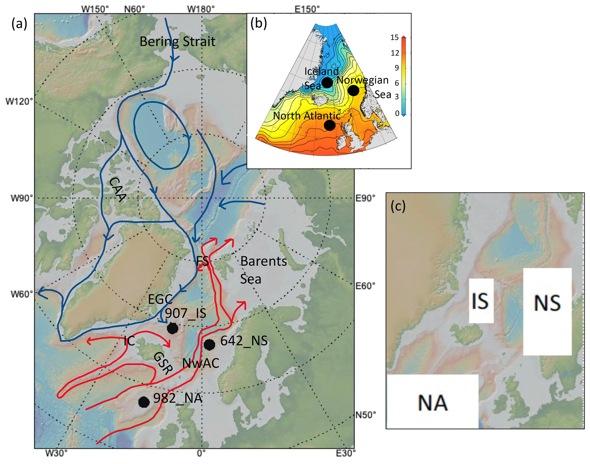
Figure 1(a) Map of the subpolar North Atlantic, Nordic Seas, and Arctic Ocean with a schematic illustration of the main surface currents (currents carrying Atlantic Water are shown in red, while currents carrying Polar Water are shown in blue). NwAC: Norwegian Atlantic Current. IC: Irminger Current. EGC: East Greenland Current. FS: Fram Strait. CAA: Canadian Arctic Archipelago. GSR: Greenland Scotland Ridge. The location of ODP Site 982 from the North Atlantic is 982_NA. The location of ODP Site 642 from the Norwegian Sea is 642_NS. The location of ODP Site 907 from the Iceland Sea 907_IS. (b) The objectively analysed mean regional ocean climatology for 1995 to 2004, represented by annual temperature (∘C) at the surface (10 m) using a quarter-degree grid (Seidov et al., 2013, 2018). The contour interval is 1 ∘C, ranging from 13 to −1 ∘C. (c) The domains over which the CMIP6 data are analysed (NA: North Atlantic; NS: Norwegian Sea; IS: Iceland Sea). The same domains are used throughout the paper for conceptual representation of the CMIP6 and Pliocene results (Figs. 6, 7, 8, and 10). The figure base is made with GeoMapApp (https://www.geomapapp.org, last access: 20 May 2021); CC BY Ryan et al., 2009.
Wind and buoyancy are the two key factors that impact the inflow of Atlantic Water to the Norwegian Sea. Wind forcing is important for the inflow of Atlantic Water across the Greenland Scotland Ridge at seasonal and interannual timescales (Bringedal et al., 2018). However, buoyancy forcing, changing seawater density due to heat (heating or cooling), and/or freshwater (evaporation, precipitation, or runoff) fluxes and the associated production of dense overflow water that must be compensated for are key at longer timescales (Furevik et al., 2007; Smedsrud et al., 2022; Talley et al., 2011). We will investigate SST (sea surface temperature) anomaly relations in the region of the North Atlantic and the Norwegian and Iceland seas at multidecadal and longer timescales – i.e. timescales when buoyancy is considered most important. Therefore, our focus is on how northern North Atlantic SST anomalies are impacted by changes in buoyancy.
Heat is continuously transported northward from the North Atlantic toward the Arctic. Due to the continuous northward transport, it is expected that a warm North Atlantic will entail warm SSTs in both in the Norwegian and Iceland seas. Alternatively, if it is cold in the North Atlantic, the Norwegian and Iceland seas are also expected to be cold. It takes 3–4 years for sea surface temperature (SST) and hence heat anomalies to travel from the North Atlantic through the Norwegian Sea (Holliday et al., 2008). Therefore, spatially incoherent SST anomalies between the seas may exist at interannual to decadal timescales. This feature has been documented in observations and Earth System Models (Årthun and Eldevik, 2016; Årthun et al., 2017). Beyond decadal timescales, however, this propagation-driven lag should in theory no longer be of importance, and the default expectation is of a spatially coherent SST relationship between the North Atlantic, the Norwegian Sea and the Iceland Sea, in line with observations (Årthun and Eldevik, 2016; Årthun et al., 2017).
Contrasting the expectation of spatially coherent SST anomalies, spatial non-coherency between SST anomalies of the North Atlantic and Norwegian Sea emerges at multidecadal timescales in the strongly forced Coupled Model Intercomparison Project (CMIP)5 RCP (representative concentration pathway) 8.5 scenario runs for future climate change (Alexander et al., 2018; Nummelin et al., 2017). These CMIP5 studies (Alexander et al., 2018; Nummelin et al., 2017; Keil et al., 2020) suggest that the expectation of spatially coherent SST anomalies between the North Atlantic and the Norwegian and Iceland seas is not valid under strongly forced high-emission scenarios and for the associated transient changes expected to take place within the next century.
We question whether the spatially non-coherent SST response seen in the CMIP5 studies is restricted to the high-emission scenario or if spatially non-coherent SST responses may also occur under less-extreme atmospheric CO2 concentrations. If it turns out that spatially non-coherent SST anomalies are also seen under less-extreme atmospheric CO2 concentrations, the validity of our expectation of spatial coherence may be limited to the observational period. To investigate whether spatially non-coherent SST responses may also occur under less-extreme atmospheric CO2 concentrations, we will use CMIP6 Shared Socioeconomic Pathway (SSP) 126 experiments and Pliocene alkenone SST reconstruction from the North Atlantic and the Norwegian and Iceland seas. During the Pliocene (5.3 to 2.6 Ma), atmospheric CO2 concentrations were close to 400 ppm on average (de la Vega et al., 2020; Bartoli et al., 2011), comparable to the present (ca. 410 ppm) and the future low-emission scenarios such as SSP126 (445 ppm by the end of the century) (Meinshausen et al., 2020; IPCC, 2021). However, it is important to keep in mind that the Pliocene climate was not forced by an abrupt CO2 increase as the future scenarios are. Rather, relatively high CO2 values existed for millions of years through the Pliocene. The SST anomaly relations in the North Atlantic and the Norwegian and Iceland seas during the Pliocene may therefore be seen as various equilibrium responses to an atmospheric CO2 content comparable to today's in contrast to the transient responses given by the CMIP model scenarios. Analysing both the SSP126 experiments and the Pliocene reconstructions therefore allows us to explore potential differences in equilibrium versus transient SST responses to a ca. 400 ppm CO2 forcing.
Furthermore, we address why spatially non-coherent SST relations may emerge and exist across different climate states, timescales, and atmospheric-CO2-forcing scenarios. As mentioned above, at multidecadal and longer timescales, the inflow of Atlantic Water to the Norwegian Sea over the Greenland Scotland Ridge is tightly connected to the density difference between the two basins (Furevik et al., 2007; Smedsrud et al., 2022; Talley et al., 2011), while wind forcing may dominate at shorter timescales (Bringedal et al., 2018). We hypothesize that, for the timescales of interest here, changing the buoyancy may be enough to push the system from spatially coherent to spatially non-coherent SST anomalies. To test this hypothesis, we perform a range of idealized sensitivity experiments using the Massachusetts Institute of Technology general circulation model (MITgcm) to investigate the impacts of changes in buoyancy forcing on the SSTs in the North Atlantic, Norwegian Sea, and Iceland Sea. These idealized experiments provide potential physical explanations for the different spatial SST relations seen in the investigated region.
By analysing variability across a wide range of timescales, we provide new perspectives on which spatio-temporal structure of SST patterns may exist under different background climate states and CO2-forcing regimes.
To confirm the basis for our expectation of spatial coherency in SST anomalies, we use data from the Met Office Hadley Centre (version 1.1) (Sect. 2.1). The future responses to SSP126 are investigated in three CMIP6 models (Sect. 2.2), while the Pliocene equilibrium response to a ca. 400 ppm CO2 forcing is documented from three ODP sites representing the North Atlantic and the Norwegian and Iceland seas (Sect. 2.3). The MITgcm experiments that test the impacts of changes in buoyancy forcing are introduced in Sect. 2.4.
2.1 Observation-based data: HadlSST
The expectation of spatially coherent SST anomalies between the North Atlantic and the Norwegian and Iceland seas is rooted in the observational period and investigations of SST anomalies at specific stations along the pathway of the North Atlantic Current (Årthun and Eldevik, 2016; Årthun et al., 2017). A comparable analysis of the observational record is done here to confirm if the expectation of spatial coherence holds when looking at averages over larger domains encompassing the North Atlantic, Norwegian and Iceland seas. The data are averaged over three box domains, as shown in Fig. 1, to represent the three sites in the Pliocene reconstructions (Sect. 2.3). The same domains are used in the CMIP6 model analysis (Sect. 2.2). We consider it to be that SST averaged over the domains better represents the variability than a single grid point. The domains are chosen as follows: to represent the site in the NE North Atlantic, we use a domain covering the northeastern part of the Subpolar North Atlantic (49–57∘ N, 35–14∘ W); to represent the site along the NwAC (North Atlantic Current), we use a box over the eastern Norwegian Sea (62.5–73∘ N, 0–16∘ E); and finally, to represent the site in the Iceland Sea, we use a box covering the major part of the Iceland Sea (66–72∘ N, 18–10∘ W). The analysed dataset is from the Met Office Hadley Centre (version 1.1) and provides monthly global SST on a 1∘ latitude–longitude grid over the period from 1870 to 2012. A detailed description of the dataset is given in (Rayner et al., 2003). In this study we use the annual mean SST to document the existing SST anomalies and the spatial relation of these between the North Atlantic and the Norwegian and Iceland seas. To investigate multidecadal timescales over the HadlSST dataset, we apply a 5-year running mean. SST anomalies are calculated relative to the mean of the respective records (1870–2012).
2.2 Transient simulations: CMIP6exp SSP126
The current generation of global climate models is available through CMIP6. CMIP6 provides a range of climate change experiments to the end of this century and beyond. To address whether or not the spatially non-coherent SST response may also occur in the future under less-extreme atmospheric-CO2-forcing scenarios than for RCP8.5, we use monthly gridded SST data from the SSP126 experiment covering the time period from 2021 to 2100 with an approximate radiative forcing of 2.6 W m−2 and a relatively low level of global warming (it is called the 2 ∘C scenario) by 2100. CO2 concentrations reach 445 ppm by 2100 (Meinshausen et al., 2020), which is at the high end of the Pliocene CO2 range (Bartoli et al., 2011; de la Vega et al., 2020). Similarly to how we treat the HadlSST data, we assess the annual mean SST from each of the model simulations. A 5-year running mean has been used to smooth the interannual variability. Because of the 5-year-running-mean filter, the time series are shown for the period 2023 to 2098. SST anomalies are calculated relative to the mean of the respective records (2021–2100).
The CMIP6 archive offers model output from many models. In this study, we have chosen to analyse three different models that have different equilibrium climate sensitivity (ECS; Meehl et al., 2020; Seland et al., 2020), leading to different amounts of warming by 2100: CNRM-ESM2-1, which has the highest sensitivity of the three models (ECS = 4.8); NorESM2-MM, which has the lowest sensitivity (ECS = 2.5); and MPI-ESM1-2-LR, which is in between in terms of sensitivity (ECS = 3). In the analysis herein, we use one member from each model (i.e. one simulation from each of the three selected models). Some additional model simulations have been included to check the responses to a more aggressive warming scenario (SSP585 experiment; NorESM2-MM), a different resolution in the atmosphere (1∘ versus 2∘; NorESM2-MM vs. NorESM2-LM), and more members (10 members compared to one single member; MPI-ESM1-2-LR). The model data are averaged over the same domains as analysed for the observational data, namely the NE North Atlantic (49–57∘ N, 35–14∘ W), the Norwegian Sea (62.5–73∘ N, 0–16∘ E), and the Iceland Sea (66–72∘ N, 18–10∘ W). SST anomalies relative to the mean of the 5-year-running-mean-filtered time series are calculated for CNRM-ESM-2-1, one of the 10 MPI-ESM1-2-LR members, and for NorESM2-MM (SSP126) and NorESM2-MM (SSP585). We focus on the SST anomalies for the three domains and the relation between these at the end of the century (2068–2098).
2.3 Pliocene SST reconstructions
To see if spatially non-coherent SST anomalies also occur between the North Atlantic and the Norwegian and Iceland seas under a past warm-climate period in equilibrium with atmospheric CO2 concentrations comparable to the SSP126 experiments, we use a compilation of previously published Pliocene alkenone SST data from three sites from the northern NE North Atlantic (ODP Site 982; 57.5167∘ N, 15.8667∘ W; 1134.2 m water depth) (Herbert et al., 2016; Lawrence et al., 2009), the Norwegian Sea (ODP Site 642; 67.255∘ N, 2.928333∘ E; 1280.9 m water depth) (Bachem et al., 2016, 2017), and the Iceland Sea (ODP Site 907; 69.24815∘ N, 12.69∘ W; 1801.5 m water depth) (Herbert et al., 2016) (Fig. 1). Each dataset covers the time interval between 5.23 and 3.13 Ma.
The index records the relative abundance of specific lipids (alkenones) synthesized by selected unicellular haptophyte algae living at or near the sea surface (e.g. Marlowe et al., 1984). Through the study of cultures, water samples, and surface sediments, it has been shown that the index changes with temperature (Prahl and Wakeham, 1987; Müller et al., 1998; Conte et al., 2006; Tierney and Tingley, 2018). All records are presented here as previously published (Herbert et al., 2016; Lawrence et al., 2009; Bachem et al., 2016, 2017), using established age models and the Müller et al. (1998) –SST calibration. The near-global and linear relationship between surface sediment values and mean annual SSTs (Müller et al., 1998) aligns closely to a culture study (Prahl and Wakeham, 1987) and has been used to calibrate and reconstruct mean annual SSTs. The standard error of estimation using this calibration is ±1.5 ∘C (Müller et al., 1998). As a biological temperature proxy, it is important to consider both the environmental and biological influences over this –SST relationship. Marked local or regional differences in the timing of alkenone production and flux to the seafloor may impart a seasonal bias to the sedimentary record (e.g. Rosell-Mele and Prahl, 2013). In a recent expansion and Bayesian analysis of the global surface sediment calibration, a stronger correlation to August–October SSTs was identified in the North Atlantic (Tierney and Tingley, 2018), i.e. in the region of our study, which may be supported by the overlap between reconstructed SSTs and autumn multi-model means for ODP Site 982 and ODP Site 642 during the KM5c interglacial at 3.205 Ma (McClymont et al., 2020). In the Nordic Seas, low salinity or high sea ice have been linked to elevated production of the C37:4 alkenone (e.g. Bendle and Rosell-Melé, 2004; Wang et al., 2021). However, this alkenone is not included in the index and was not recorded at values of concern at ODP Site 642 (Bachem et al., 2017).
The sampling resolution of the original records varies; for Site 907 (Iceland Sea), the mean original temporal resolution was ca. 2600 years; however, from 3.33 to 3.16 Ma, the spacing between measurements ranges from 4000 to 70 000 years; for Site 642 (Norwegian Sea), the mean resolution was ca. 2500 years between 3.13 and 3.49 Ma and ca. 7200 years between 3.49 and 5.23 Ma; and for Site 982, it was ca. 2100 years between 3.13 and 4.03 Ma and ca. 40 800 years between 4.03 and 5.23 Ma. To enable direct comparison between sites, independent of differences in temporal resolution and absolute ages for the raw data points, each dataset has been resampled every 100 kyr between 5.23 and 3.13 Ma using a linear integration function in AnalySeries (Paillard et al., 1996). SST anomalies are calculated relative to the mean of the respective resampled records (5.23–3.13 Ma). The 100 kyr resampling interval is chosen to put focus on the long-term trends of each record and the background climate state upon which the shorter-term orbital variability is superimposed (Fig. 2). The shorter-term orbital variability is not well-enough resolved by all records throughout the investigated time interval to allow for a higher-resolution resampling. Hence, given the timescales considered here, the SST anomaly relations are unlikely to be orbitally forced. Furthermore, focusing on the mean state of longer intervals (the shortest time interval is 200 000 years) rather than point-to-point comparison also minimizes the impact of uncertainties from age models. Pliocene chronologies are mostly constrained by tuning to LR04 (Lisiecki and Raymo, 2005) and/or using tie points from magnetic reversals. The tuning error is generally considered to be no more than a few thousand years but may exceed 10 kyr prior to 4.3 Ma due to less-certain obliquity variance (Lisiecki and Raymo, 2005). At the timescales considered here, such errors are acceptable.
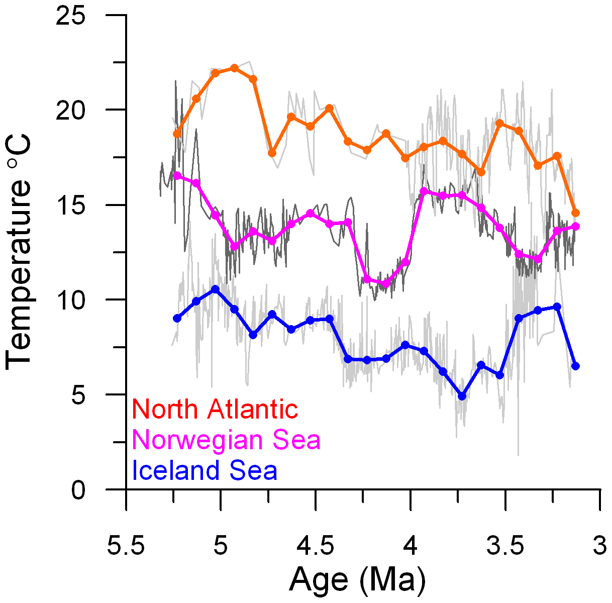
Figure 2Original SST reconstructions from the North Atlantic and the Norwegian and Iceland seas (grey tones) (Bachem et al., 2016, 2017; Herbert et al., 2016; Lawrence et al., 2009) with 100 kyr resampled datasets superimposed (North Atlantic (red), Norwegian (magenta), and Iceland seas (blue)).
2.4 Model set-up and reference experiments
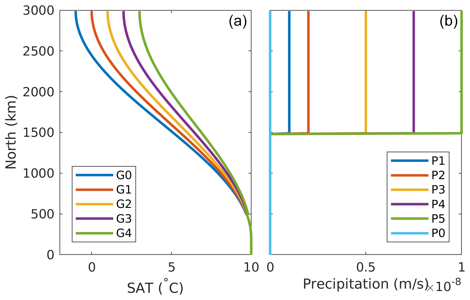
We use an idealized-topography configuration of the MITgcm (Marshall et al., 1997) to investigate the SST relationships in the study area under a range of buoyancy forcings (Fig. 1). The set-up (Fig. 3) is a Nordic-Seas-like basin separated from a truncated North-Atlantic-like source water region by a 1000 m deep ridge. Both basins are flat-bottomed, with 2000 m depth, and are surrounded by sloping sides. The model domain is closed. The boundary conditions and prescribed forcings are the following: there is a restoring boundary condition in the south maintaining the reservoir of Atlantic source water. The temperature is restored to a temperature of TA= 6 ∘C and a salinity of 35 psu, with a restoring strength of 40 W m−2 and a timescale of 1 month. In addition, SSTs are restored toward atmospheric temperatures (SATs) through the surface heat flux which is parameterized as , where G= 40 W m−2 C−1. There is no interactive atmosphere. There is a constant, uniform freshwater input in the form of precipitation north of the ridge. Mechanical forcing is provided by a constant-in-time prescribed wind field (W) with westerlies over the North Atlantic and easterlies over the Nordic Seas field. The latitude of zero wind stress curl is in the middle of the Atlantic region, with cyclonic wind stress to the north and anti-cyclonic wind stress to the south.
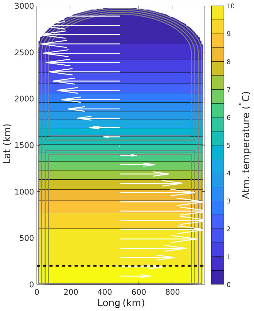
Figure 3The model set-up. Grey contours outline the bathymetry (every 300 m), colours show the SAT (profile G1 in Fig. 4), and white arrows represent the wind forcing. Fig. 4 provides an overview of the different buoyancy (SAT and freshwater) forcings used for the experiments. South of the dashed black line, salinity is restored to 35 psu, and oceanic temperature is restored to 6 ∘C.
The horizontal resolution is 10 km, and there are 30 vertical layers; the upper 20 layers are 50 m thick, and the deepest layers are 100 m thick. Water density is calculated using the formula from Jackett and McDougall (1995), with a constant Coriolis parameter, s−1, and vertical diffusivity and viscosity of m2 s−1. Convection is parameterized with implicit vertical diffusion; the diffusivity increases to 1000 m2 s−1 for statically unstable conditions. Horizontal viscosity is parameterized using the Smagorinsky closure (Smagorinsky, 1963); typical values are 30 m2 s−1 for the boundary current region. Temperature and salinity are advected using a third-order flux-limiting scheme.
Since one of the key drivers for inflow of Atlantic Water to the Norwegian Sea is buoyancy forcing and the production of dense overflow water that must be compensated for (Furevik et al., 2007), we change the SAT (G) and the freshwater (in the form of precipitation) (P) north of the ridge to study the impact of buoyancy forcing on the relationships between SSTs in the North Atlantic, Norwegian Sea, and Iceland Sea. The SAT and freshwater are changed as shown in Fig. 4 and Table 1. Note that the SAT over the restoring region is the same for all experiments. The idealized model is run for 30 years to near steady state, and we present results from the last 5 years of the runs, which are compared to the results from the relevant reference experiment. We are therefore not studying transient changes but differences between equilibrium states.
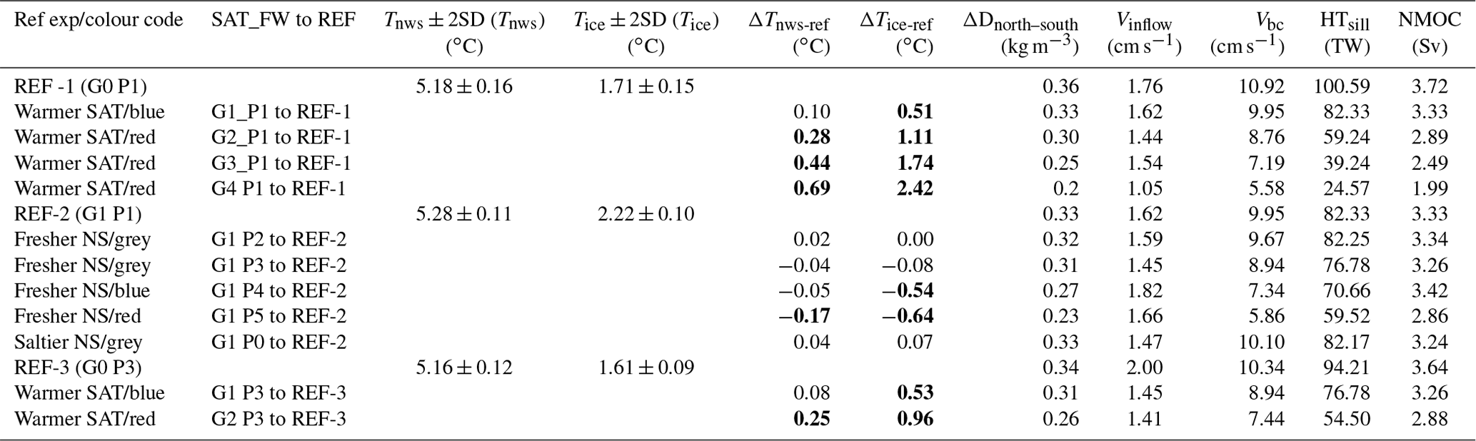
Table 1Selected output from the MITgcm idealized model experiments, where buoyancy is changed by changing either SAT (G) or freshwater in the form of precipitation (P). SAT is atmospheric temperature forcing (Fig. 4), FW is freshwater forcing (Fig. 4), Tnws and Tice are the sea surface temperature of the boundary current or the Norwegian Sea and the interior or the Iceland Sea (Fig. 5) for the three reference experiments. ΔTnws-ref and ΔTice-ref ref are the temperature difference between the experiment and the corresponding reference experiment for the boundary current or the Norwegian Sea and the interior or the Iceland Sea, respectively. The numbers are marked in bold if the temperature difference exceeds the 2 × SD of the reference experiment. ΔDnorth–south is the density difference between north (averaged over 2000–2500 km) and south (averaged over 500–1000 km) of the ridge within each experiment over the full depth. Vinflow is the mean inflow velocity across the sill (cm s−1) (at 1500 km), Vbc is the mean velocity in the boundary current (cm s−1) (average for the Norwegian Sea, as defined by the pink box in Fig. 5), HTsill is the net heat transport across the sill (TW) (at 1500 km), and NMOC (Sv) is the maximum overturning streamfunction at the sill (at 1500 km). Ref exp is the corresponding reference experiment which the experiment is compared against. The three different SST anomaly relations identified are colour coded (grey – spatial coherence; red – Norwegian Sea and Iceland Sea SST anomaly different from that of the North Atlantic; blue – a temperature change larger than 2 × SD in relation to the reference experiment in the Iceland Sea and less than 2 × SD in relation the reference experiment change in the Norwegian Sea and North Atlantic, considered to be a representation of an Iceland Sea SST anomaly different from the North Atlantic and the Norwegian Sea).
Buoyancy changes are forced north of the ridge due to the nature of the model set-up. The restoring boundary conditions in the south are also a forcing, representing both the (infinite) source of Atlantic Water and the experiment's energy source (heat and buoyancy input). As the surface forcing is applied north of the ridge, water mass transformation takes place, and a consistent ocean circulation is set up, including the setting of the hydrography of the different regions. The southern boundary energy input and northern surface heat loss balance when the model has reached (quasi)-equilibrium. The northern and southern regions are accordingly equally important for the experiments.
We want to investigate the responses to changes in buoyancy caused by either an SAT or a freshwater change. In addition, we want to see if the initial state of the ocean impacts the response to a SAT change, specifically testing if the response differs if we start out from the fresher Nordic Seas. Therefore, we define three reference experiments, namely REF-1 (G0 and P1), REF-2 (G1 and P1), and REF-3 (G0 and P3) (Table 1). REF-1 is set up to investigate the oceanographic responses to a gradually decreasing SAT gradient between the North Atlantic and the Nordic Seas under constant freshwater forcing by increasing the SATs over the Nordic Seas. For the REF-2 experiments, the buoyancy is changed by gradually increasing the freshwater over the Nordic Seas, while SAT is kept constant. The REF-3 experiments are similar to the REF-1 experiments in the sense that SAT over the Nordic Seas is increased; however, the initial state of the Nordic Seas is fresher for REF-3 than for REF-1. Hence the REF-3 experiments are set up to see how the initial state of the ocean may impact the responses to increased SAT over the Nordic Seas.
The combination of the prescribed wind stress and the steep yet sloping coastal boundary supports a cyclonic boundary-intensified circulation around the Nordic Seas. The reference experiments have an ocean circulation which represents the main characteristics of the North Atlantic (south of the ridge), with an anticyclonic gyre in the subpolar latitudes and a cyclonic gyre further south. The buoyancy forcing from the prescribed surface temperature and salinity results in a gradual meridional temperature decrease and a similar salinity decrease, mimicking northern heat loss and freshwater input (Fig. 5). The thermal forcing dominates, and there is net northern buoyancy loss. There is warm and saline inflow to the Nordic-Seas-like basin and a colder and fresher outflow. The densest and coldest water is found in the relatively motionless and weakly stratified interior of the Nordic Seas. The overall temperature contrast between the dense-water interior and the Atlantic source water region reflects the temperature range of the prescribed surface air temperature. Waters are continuously exchanged between the buoyant boundary current and the interior by lateral eddy mixing. Heat is thus not only lost from the boundary current by air–sea interaction but also by lateral heat loss to the interior, where it is also given up to the atmosphere.
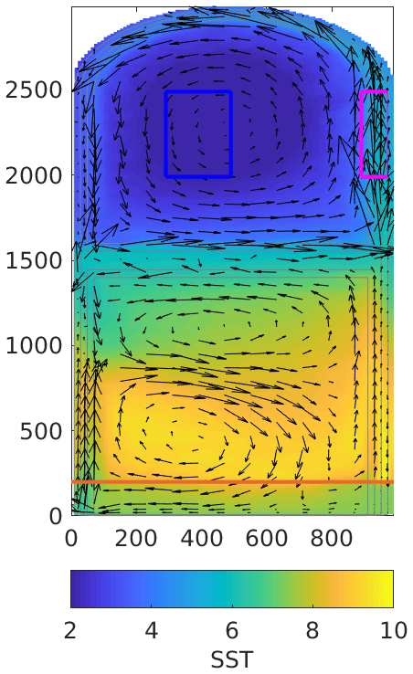
Figure 5Example of SSTs (colours) and upper 500 m ocean circulation (black arrows) for the MITgcm experiments. The indicated boxes show the areas used to calculate the SSTs of the Norwegian Sea (pink) and the Iceland Sea (blue) used in Table 1. The domains are set for the results to be comparable to the reconstructions, observations, and CMIP6 results. However, since the MITgcm is idealized, the domains can not be identical to the domains defined in Sect. 2.1. The North Atlantic restoring region equals the area south of the red line.
For the MITgcm, the Norwegian Sea domain is defined as a box in the eastern boundary current region, while the Iceland Sea domain is represented by the interior ocean north of the ridge (Fig. 5). The definition of these domains, as the domains used for the observations and CMIP6 results (Sect. 2.1; Fig. 1), is directed by the location of the Pliocene sites, representing the Norwegian boundary current and the interior Iceland Sea.
The definition of the North Atlantic domain is somewhat different; it is, for simplicity, defined as the North Atlantic restoring region (Fig. 5), restored to 6 ∘C for all experiments (Fig. 4a). With this restoring, the state of the North Atlantic source water that eventually becomes the inflow to the Nordic Seas is essentially known. Also, the model North Atlantic is much less directly impacted by the prescribed changes in buoyancy forcings than the Nordic Seas (Fig. 4) and is also less impacted in consequence, as evident in Fig. 9. Directly related, it is the relative temperature (density) difference of the model ocean that constrains the flow and thus the results. The nonlinearity of the equation of state will only be in effect for large excursions in the absolute values of the restoring temperature and salinity between the different experiments.
In short, the MITgcm experiments assess the state of the Nordic Seas, including that of the Norwegian and Iceland seas, relative to that of the North Atlantic. The summary of experiments in Table 1 reflects this relative perspective.
We identify spatially coherent and non-coherent SST anomaly relationships between the North Atlantic and the Norwegian and Iceland seas by comparing the temperature of the sensitivity experiment with the relevant reference experiment. Change in a region is classified as an SST anomaly when the temperature change between two experiments exceeds 2σ(SSTreference_experiment), with σ calculated after temporally averaging the model SSTs. The North Atlantic is restored to constant temperatures as mentioned above. Even if it deviates (slightly) within what is allowed for by the restoring (see Sect. 2.4), it remains essentially constant and non-anomalous. Thus, as also alluded to above, change in the SST anomaly relationship between the three regions exists if there is a temperature change in either the Norwegian Sea or the Iceland Sea, or in both, larger than 2σ.
First, the relations between SST anomalies in the North Atlantic and the Norwegian and Iceland seas, as seen in HadlSST (multidecadal timescales), the low-emission-future-scenario runs (CMIP6 SSP126; multidecadal timescale), and Pliocene SST reconstructions (over several 100 kyr), are presented. Thereafter, we present the results of the idealized experiments that tested the impact of changes in buoyancy forcing on the SST anomalies. The Pliocene reconstructions are site specific but are considered to provide a reasonable representation of their respective regions, while the observation and model data are regional averages. Somewhat larger amplitudes of the recorded SST anomalies may therefore be expected to be seen in the reconstructions.
3.1 SST anomaly relations in observation-based data: HadlSST
On multidecadal timescales the annual SST anomaly, as seen in the HadlSST dataset, varies between −0.8 and +0.8 ∘C (Fig. 6). As described in the introduction, the spatially non-coherent SST anomaly signal seen on shorter timescales should in theory no longer be of importance on multidecadal timescales, and we see a spatially coherent SST anomaly relationship between the North Atlantic, the Norwegian Sea, and the Iceland Sea (Fig. 6). The spatially coherent SST anomaly relationship between the North Atlantic, the Norwegian Sea, and the Iceland Sea is robust, showing positive and significant correlations between the detrended time series (both the Norwegian Sea and the Iceland Sea are correlated with the North Atlantic). The relationship also holds for different filtering of the time series, i.e. running means with a 5-year window, 10-year window, and 15-year window (not shown). On multidecadal timescales, these regions follow, to a large extent, the Atlantic multidecadal variability (AMV), with a warm phase in 1930–1970 and a cold phase in 1970–1990 (Knight et al., 2005).
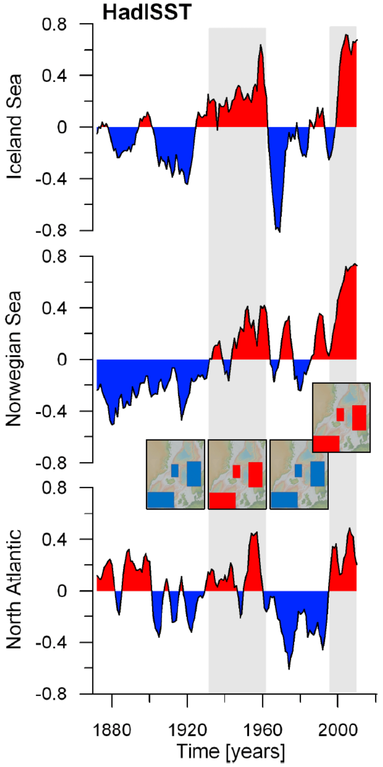
Figure 6Annual SST anomalies for the North Atlantic and the Norwegian and Iceland seas based on HadlSST data. SSTs have been averaged over the three box regions before calculating the anomalies: 49–57∘ N and 14–35∘ W (North Atlantic), 62.5–73∘ N and 0–16∘ E (Norwegian Sea), and 66–72∘ N and 10–18∘ W (Iceland Sea). A running mean with a 5-year window has been applied to the time series, and the anomalies are shown relative to the mean of the 5-year-running-mean-filtered time series (1870–2012). The map inserts provide a conceptual representation of the results, with blue (red) boxes representing cold (warm) SST anomalies for the North Atlantic and the Norwegian and Iceland seas. The grey bars highlight the periods with positive spatially coherent SST anomalies. The base for the map inserts is made with GeoMapApp (https://www.geomapapp.org/); CC BY Ryan et al., 2009.
3.2 Future SST anomaly relations – CMIP6exp: SSP126
The three models, CNMR-ESM2-1, MPI-ESM1-2-LR, and NorESM2-MM, show different results, both with respect to their SST climatology and the SST anomalies in each region of interest for the end of the 21st century (the last 3 decades, 2068–2098) (Fig. 7). The mean SST of the 5-year-running-mean-filtered time series (2023–2098) of the NE North Atlantic is fairly similar in the three models, but that of the Norwegian Sea differs to some extent, with MPI-ESM1-2-LR being warmest (9.5 ∘C), NorESM2-MM being coldest (6.8 ∘C), and CNRM-ESM2-1 being in between (7.8 ∘C). The mean SST in the Iceland Sea differs to a large extent among the three models, again with MPI-ESM1-2-LR being warmest (5.6 ∘C) and NorESM2-MM being coldest (0 ∘C).
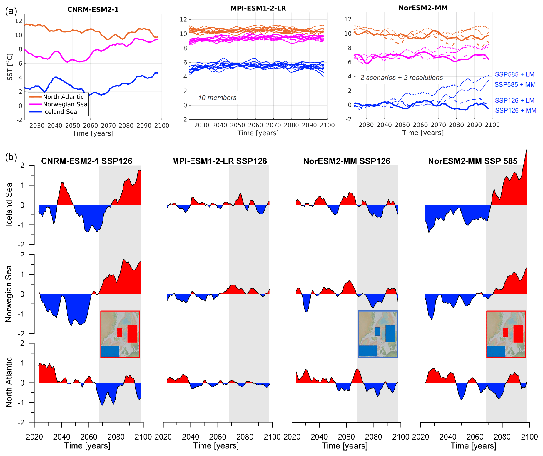
Figure 7(a) Annual mean SST based on CMIP6 future scenario SSP126, representing the North Atlantic (red) and the Norwegian (magenta) and Iceland seas (blue). SSTs have been averaged over the same box regions as described in Fig. 3. CNRM-ESM2-1 displays 1 member, MPI-ESM2-2-LR displays 10 members, and NorESM2-MM displays two different scenarios (SSP126 – thick curves; SSP585 – thin curves) and two different atmospheric resolutions (medium – solid curves; low – dashed curves). A running mean with a 5-year window has been applied to the time series. (b) SST anomalies relative to the mean of the 5-year-running-mean-filtered time series (2023 to 2098) from CNRM-ESM-2-1 (SSP126), one of the 10 MPI-ESM1-2-LR members, and from NorESM2-MM (SSP126) and NorESM2-MM (SSP585). We focus on the SST anomalies for the three domains and the relation between these at the end of the century (last 3 decades, 2068–2098, marked by the grey bars). The map inserts provide a conceptual representation of the results, with blue (red) boxes representing cold (warm) SST anomalies for the North Atlantic and the Norwegian and Iceland seas. The individual members of MPI-ESM1-2-LR SSP126 cannot be distinguished from each other. Therefore, we have not added a map insert for the member presented. The base for the map inserts is made with GeoMapApp (https://www.geomapapp.org/); CC BY Ryan et al., 2009.
CNRM-ESM2-1 shows larger SST anomalies for the Norwegian Sea and the Iceland Sea than the two other models (Fig. 7b). This is consistent with CNRM-ESM2-1 being the most sensitive, or more rapidly responding, model (as described in Sect. 2.2). Based on CNRM-ESM2-1, we find a dominantly cold SST anomaly in the North Atlantic and a warm SST anomaly in the Norwegian and the Iceland seas toward the end of the 21st century (2068–2098). Thus, for the SSP126 scenario, CNRM-ESM2-1 suggests that the North Atlantic SST anomaly will differ from the SST anomalies of the Norwegian and Iceland seas at the end of the 21st century.
Compared to the CNRM-ESM2-1 results, both MPI-ESM1-2-LR and NorESM2-MM show much smaller SST anomalies at the end of the 21st century relative to the model annual mean SST over the next century (Fig. 7b). Considering 10 different members from MPI-ESM1-2-LR, we find that the results from the individual members do not differ to a large extent (Fig. 7a); none of the members show anything but minor annual mean SST variability for any of the domains. The difference between the members is less than the amplitude of the changes in CNRM-ESM2-1. On the other hand, considering a more aggressive scenario (SSP585) for NorESM2-MM, we find a clear warm anomaly in the Norwegian and Iceland seas (Fig. 7b). A cold, but small, SST anomaly is seen for the North Atlantic. Hence, the sensitivity of the model impacts the result. Furthermore, we find that lowering the horizontal resolution in the atmosphere entails higher SSTs in the Iceland Sea at the end of the century relative to the results from the model version with a higher horizontal resolution in the atmosphere. A lower horizontal resolution in the atmosphere does not, however, have a clear effect on the SSTs of the Norwegian Sea or the North Atlantic (Fig. 7a).
The spatially incoherent SST anomaly relationship found in CNRM-ESM2-1 SSP126 and NorESM2-MM SSP585 in the last 3 decades (2068–2098) (Fig. 7) is sensitive to the chosen period and is not robust over the whole projected period (2023–2098). Correlations are overall nonsignificant between the time series from the three regions. Positive correlations are indicated for NorESM2-MM SSP585 (both the Norwegian Sea and the Iceland Sea are correlated with the North Atlantic), but only if the time series are detrended. In the latter case, the spatially incoherent SST anomaly relationship in the last 3 decades is not found in NorESM2-MM SSP585.
3.3 SST anomaly relations in Pliocene SST reconstructions
The relation between SST anomalies of the North Atlantic, Norwegian Sea, and Iceland Sea is not constant through the Pliocene. The following two different spatially non-coherent SST anomaly relations are documented: (1) the Norwegian Sea SST anomaly differs from the SST anomalies of the North Atlantic and the Iceland Sea, either with a warm Norwegian Sea anomaly corresponding with a cold anomaly in the North Atlantic and Iceland Sea (first yellow period in Fig. 8; 3.63–3.93 Ma) or the opposite, with a cold anomaly in the Norwegian Sea corresponding to a warm anomaly in the North Atlantic and Iceland Sea (second yellow period in Fig. 9; 4.73–4.93 Ma); (2) a cold anomaly in the North Atlantic and the Norwegian Sea corresponds to a warm anomaly in the Iceland Sea (blue period in Fig. 9; 3.23–3.43 Ma). All these Pliocene SST anomaly relationships are different from what we see in the CMIP6 future runs (warm Norwegian Sea and Iceland Sea, cold North Atlantic). In addition to the spatially non-coherent SST anomaly relations, there are three time periods during the Pliocene that show a spatially coherent SST anomaly relationship, comparable to what we find for the observation-based data (grey time periods in Fig. 8; 4.03–4.33, 4.43–4.63, and 5.03–5.23 Ma).
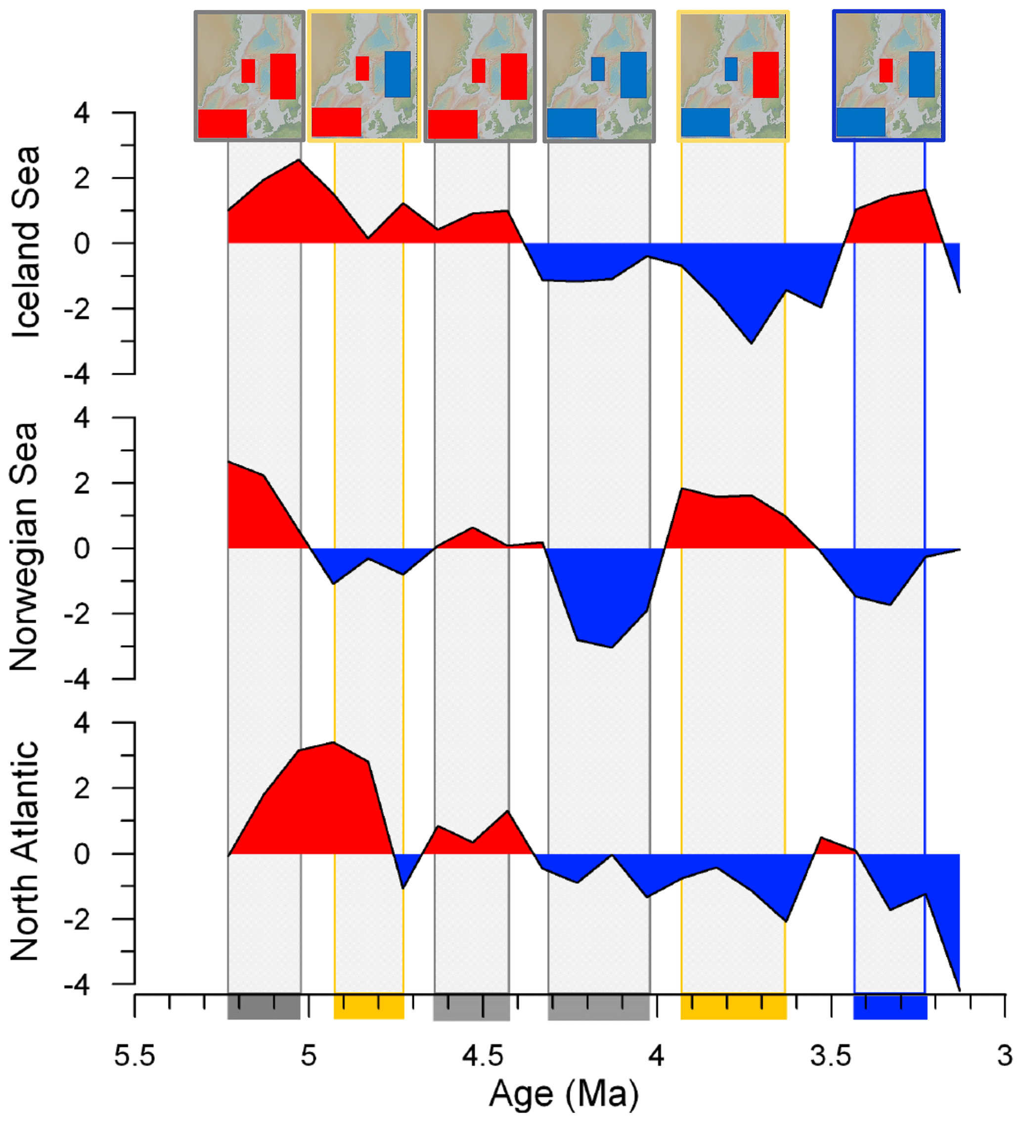
Figure 8Pliocene SST anomalies (∘C, relative to the mean of the 100 kyr resampled records). The different SST anomaly relations identified are colour coded (grey boxes – spatial coherence; blue box – Iceland Sea SST anomaly differing from the North Atlantic and Norwegian Sea SST anomalies; yellow boxes – Norwegian Sea SST anomaly differing from the North Atlantic and Iceland Sea SST anomalies). Conceptual illustrations of the respective SST anomaly relations for each interval are shown for all identified scenarios, with blue (red) boxes representing cold (warm) SST anomalies for the North Atlantic and the Norwegian and Iceland seas (from left to right: positive spatial coherence; cold Norwegian Sea, warm North Atlantic and Iceland Sea; positive spatial coherence; negative spatial coherence; warm Norwegian Sea, cold North Atlantic and Iceland Sea; warm Iceland Sea, cold North Atlantic and Norwegian Sea). The base for the map inserts is made with GeoMapApp (https://www.geomapapp.org/); CC BY Ryan et al., 2009.
3.4 Buoyancy-forced SST anomaly relationships – results from the MITgcm idealized experiments
By changing the buoyancy forcing as shown in Figs. 4 and 5, we can produce the following three different spatial SST anomaly relationships in the idealized model: spatially coherent SST anomalies in all three regions (grey experiments, Table 1 and Fig. 9b), Norwegian Sea and Iceland Sea SST anomalies that are different from the North Atlantic (red experiments, Table 1 and Fig. 9), and an Iceland Sea SST anomaly that differ from the North Atlantic and Norwegian Sea SST anomalies (blue experiments, Table 1 and Fig. 9). Hence, these idealized experiments can capture two of the three SST anomaly relations found during the Pliocene (grey and blue time periods in Fig. 8) and the SST anomaly relationship found in the CMIP6 future runs (Fig. 7). Table 1 summarizes the experiments.
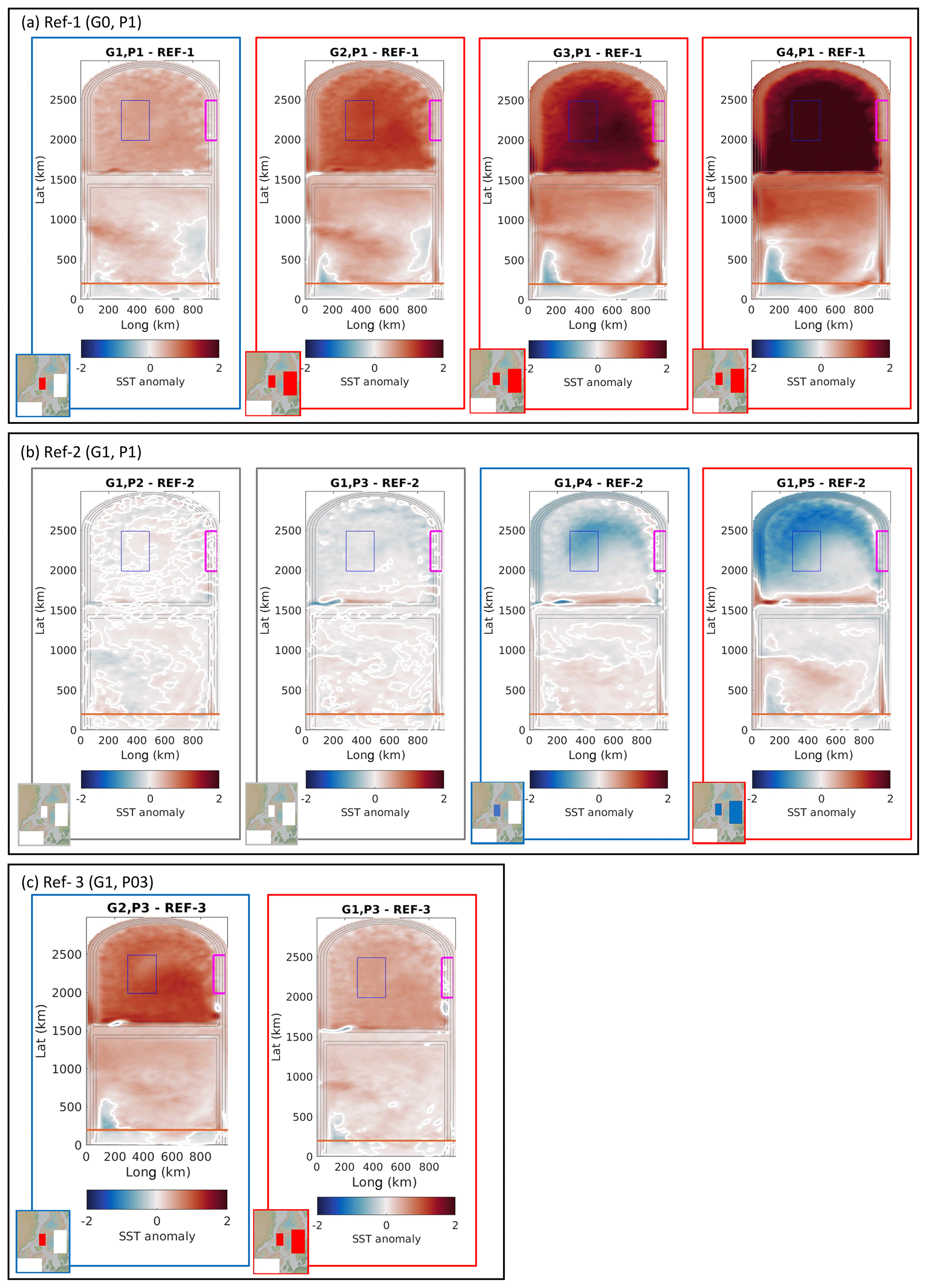
Figure 9SST anomalies seen in MITgcm idealized experiments. White marks the zero-contour line. (a) SST anomalies relative to REF-1, where freshwater is kept constant at P1 while SAT is gradually increased (G1–G4). (b) SST anomalies relative to REF-2, where SAT is kept constant at G1 while freshwater is gradually increased (P2–P5). (c) SST anomalies relative to REF-3, where freshwater is kept constant at P3 while SAT is increased (G1 and G2). Surrounding blue boxes represent an Iceland Sea SST anomaly that is spatially incoherent with the North Atlantic and Norwegian Sea anomalies. The SST anomaly seen in the Iceland Sea exceeds 2 × SD in relation to the relevant reference experiment. Surrounding red boxes represent a North Atlantic SST anomaly that is spatially incoherent with the anomalies of the Norwegian and Iceland seas. The SST anomalies seen in the Norwegian and Iceland seas exceed 2 × SD in relation to the relevant reference experiment. Surrounding grey boxes represent spatially coherent SST anomalies between the three regions (none of the SST anomalies exceed 2 × SD in relation to the relevant reference experiment). A conceptualized representation of the resulting SST anomaly relations is shown by the map inserts, where blue (red) boxes represent cold (warm) SST anomalies for the North Atlantic, Norwegian Sea, and Iceland Sea. White boxes are used if the SST anomalies in the Norwegian and/or Iceland seas are less than 2 × SD in relation to the relevant reference experiment and for the North Atlantic (where the restoring will dampen the potential temperature change so that the temperature change is close to constant (see Sect. 2.4 for further details)). The base for the map inserts is made with GeoMapApp (https://www.geomapapp.org/); CC BY Ryan et al., 2009.
The first set of four experiments has the same freshwater forcing (P1) but a decreasing SAT gradient (i.e. increasing SAT over the Nordic Seas (G1–G4)) relative to REF-1. As SAT increases over the Nordic Seas, the SST pattern shifts from the Iceland Sea SST anomaly being different from the North Atlantic and the Norwegian Sea (G1) to the North Atlantic SST anomaly being different from the Norwegian and Iceland seas (G2–G4) (Fig. 9a).
In the next set of experiments, SAT is kept constant (G1) while the freshwater over the Nordic Seas is increased (P2–P5) relative to REF-2. With increasing freshwater over the Nordic Seas, the SST pattern shifts from one of spatial coherence (P2 and P3) to the Iceland Sea SST anomaly being different from the North Atlantic and the Norwegian Sea (P4) to the North Atlantic SST anomaly being different from the Norwegian and Iceland seas (P5) (Fig. 9b).
In the last set of experiments, the decreasing SAT gradient experiments (G1–G2) are repeated with fresher Nordic Seas (P3) relative to REF-3. As for REF-1, the SST pattern shifts from the Iceland Sea SST anomaly being different from the North Atlantic and the Norwegian Sea (G1) to the North Atlantic SST anomaly being different from the Norwegian and Iceland seas (G2) when we increase the SAT over the Nordic Seas (Fig. 9c).
In addition to identifying the SST anomalies in the MITgcm experiments, information about the density difference over the ridge, the mean inflow velocity across the sill, the mean velocity in the boundary current, the net heat transport over the sill, and the maximum overturning streamfunction at the sill is extracted for each experiment (Table 1). This information will be used in the discussion, exemplifying oceanographic responses to specific buoyancy changes as seen in the MITgcm experiments.
Reducing the SAT gradient, i.e. warming the atmosphere over the Nordic Seas, reduces the heat loss from the ocean and warms the SSTs in the Nordic Seas. Compared to the reference experiment, the following are smaller: the north–south density difference, the mean inflow velocity across the ridge, the boundary current velocity in the Nordic Seas, the net heat transport across the sill, the maximum overturning circulation across the sill, and the lateral eddy heat transport in the Nordic Seas (Table 1). The weaker ocean circulation transports less heat to the Nordic Seas. In addition, as the Norwegian Sea boundary current is slower in warmer experiments, the water of the boundary current experiences more cooling as it travels the Nordic Seas, allowing for a larger heat loss in the Norwegian Sea region.
For the experiments with a small SAT change (G1 relative to REF-1 and G1 relative to REF-3; blue experiments in Table 1 and Fig. 9a, c), the increased heat loss from the Norwegian Sea boundary current and the decreased poleward heat transport are partly able to compensate for the increased atmospheric warming in the Norwegian Sea, and thus there is no temperature change larger than 2 × SD in relation to the relevant reference experiment in the Norwegian Sea. However, this is not the case for the Iceland Sea, where the SSTs increase. We consider this result to be representative for a situation when the SST anomaly of the Iceland Sea differs from the North Atlantic and Norwegian Sea SST anomalies – hence, when there is an SST field that breaks the expectation of spatially coherent SST anomalies. The amplitude of the MITgcm Iceland Sea SST anomaly is, in this case (G1 relative to REF-1 and G1 relative to REF-3), approximately one-third of the Iceland Sea SST anomaly reconstructed for the Pliocene (3.43 to 3.23 Ma) when the SST anomaly of the Iceland Sea differs from the North Atlantic and Norwegian Sea SST anomalies.
For larger SAT warming over the northern basin (G2–G4 relative to REF-1 and G2 relative to REF3; red experiments; Table 1 and Fig. 9a, c), both the Iceland and Norwegian seas experience a temperature increase larger than 2 × SD in relation to the relevant reference experiment. There is more warming in the Iceland Sea than in the Norwegian Sea, and the difference increases with larger SAT warming (i.e. weaker SAT gradients). Thus, the absolute temperature for the Iceland Sea is more like the Norwegian Sea for a warmer atmosphere over the Nordic Seas. The larger SST change in the Iceland Sea can be explained by a combination of reduced heat transport to the Nordic Seas and a slower Nordic Seas boundary current, which allows for larger heat loss in the Norwegian Sea region and more cooling of the water as it travels the Nordic Seas. The increased heat loss and decreased poleward heat transport counteract the general atmospheric warming over the Norwegian Sea more than over the Iceland Sea. The amplitude of the SST anomalies in the Iceland and Norwegian seas, as seen in CNRM-ESM2-1 SSP126 and NorESM-MM SSP528 at the end of the century, is within the range of the respective MITgcm SST anomalies.
Increasing the north–south salinity gradient across the sill (REF-2 experiments) gives similar results; no SST change larger than 2 × SD in relation to REF-2 is found in the two regions for small changes in freshwater forcing (P2–P3 relative to REF2), an SST change is found only in the Iceland Sea for medium changes in freshwater forcing (P4 to REF-2), and SST changes are found in both the Iceland and Norwegian seas for the largest changes in freshwater forcing (P5 to REF-2, equal to a freshwater increase from 1 to m s−1 (Fig. 4)) (Table 1 and Fig. 9b). Fresher Nordic Seas weaken the north–south density gradient, which weakens the poleward heat transport and the boundary current velocity. The slower boundary current allows for more heat loss to the atmosphere in the Norwegian Sea, and the region cools. In these experiments, there is no prescribed warming of the atmosphere, so temperature change is only set by the changes in ocean circulation. The slower boundary current also reduces the eddy heat fluxes from the boundary to the interior, and hence, the Iceland Sea region also cools. As for the experiments where we increase the atmospheric temperature over the Nordic Seas, the Iceland Sea SST anomaly in the respective Pliocene case is larger than the MITgcm SST anomaly response to a medium freshwater change (P4 to REF-2). The MITgcm response to the largest freshwater forcing (P5 to REF-2) is at the lower end of the SST anomalies seen for the CMIP6 models at the end of the century.
Within the investigated parameter space, we have not found a situation where the increased heat loss and decreased poleward heat transport more than compensate for the increased atmospheric warming so that the Norwegian Sea temperature change is opposite to that of the other two regions (i.e. the situation seen for the yellow time periods in Fig. 8).
We have limited our study to the impact of buoyancy forcing on SST relationships. Using a similar model configuration, Spall (2011, 2012) report on the impact of changing sill depth on the temperature of the interior region (the inflowing temperature; i.e. Norwegian Sea temperature is assumed to equal that of the source region). A deeper sill increases the temperature of both the boundary current and the interior of the Nordic Seas. The difference in temperature between these two regions decreases for larger sill depths. The changes are associated with a strengthening of the meridional overturning circulation across the sill and, to a lesser extent, an increase in heat transport across the sill.
In this study, we have identified the following four different SST anomaly relations (Fig. 10): (1) the SST anomalies of the North Atlantic and the Norwegian and Iceland seas are spatially coherent (at multidecadal timescales in the observation-based records and over hundreds of thousands of years for three Pliocene intervals (4.03–4.33, 4.43–4.63, and 5.03–5.23 Ma; Figs. 6 and 8), (2) the Iceland Sea SST anomaly is different from the North Atlantic and Norwegian Sea SST anomalies (over 200 000 years in the Pliocene – 3.23–3.43 Ma; Fig. 8), (3) the North Atlantic SST anomaly is different from the SST anomalies of the Norwegian and Iceland seas (at multidecadal timescales at the end of the 21st century, Fig. 7), and (4) the Norwegian Sea SST anomaly is different from the North Atlantic and Iceland Sea SST anomalies (again over hundreds of thousands of years during the Pliocene – 3.63–3.93 and 4.73–4.93 Ma; Fig. 8). From our idealized MITgcm experiments for the North-Atlantic–Nordic-Seas region, three of the four different SST anomaly relations (1, 2, and 3) could be reproduced by changing the buoyancy forcing (atmospheric temperature and freshwater; Table 1 and Figs. 9, 10). Our results thus suggest a key role for buoyancy forcing in setting the SST anomaly variability in the northern North Atlantic.
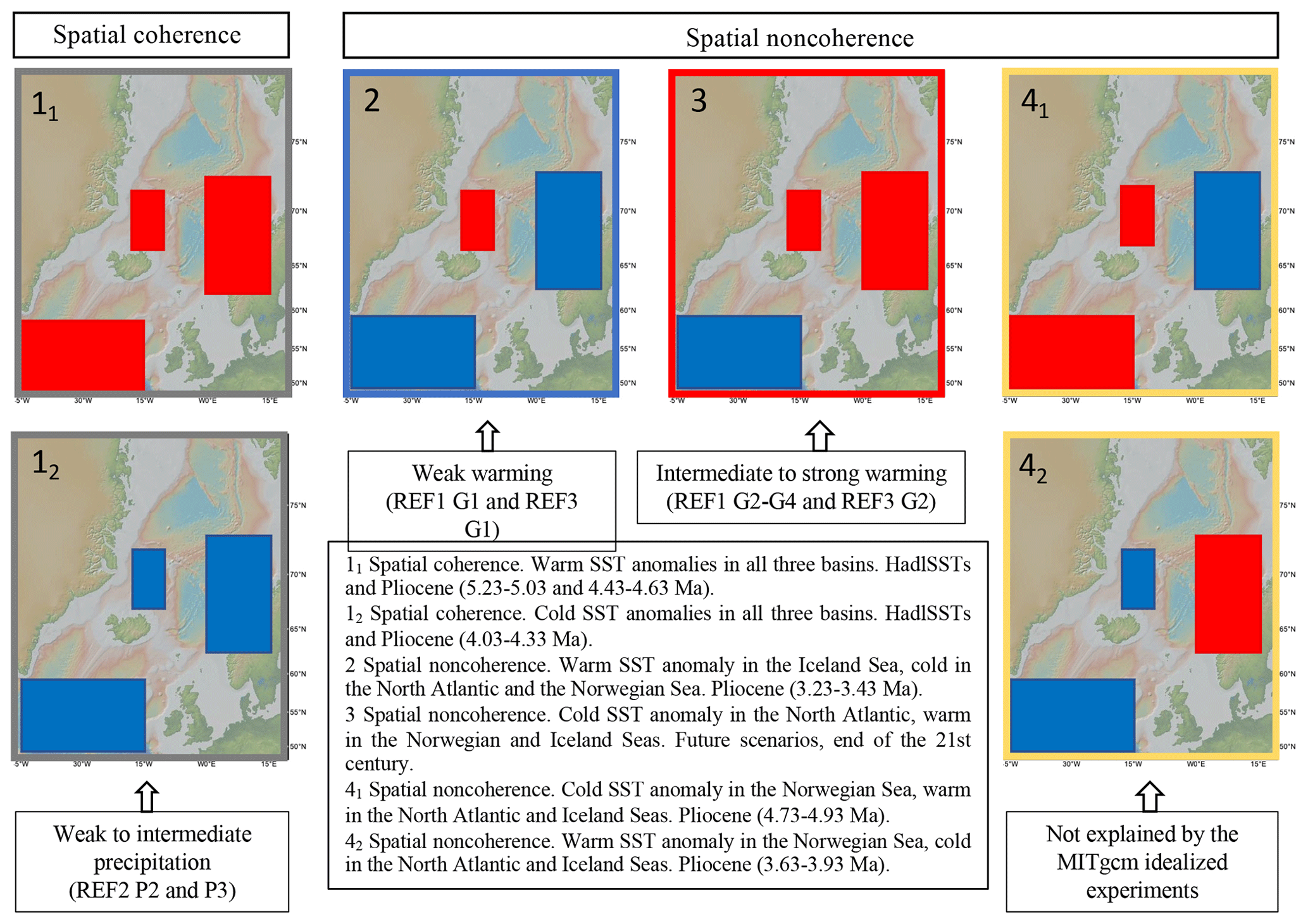
Figure 10Conceptual illustration of the identified SST anomaly relations, showing for which period the explicit SST anomaly relations are seen and which MITgcm idealized experiments resulted in the same type of SST relationships. Blue (red) boxes representing cold (warm) SST anomalies. The background maps are made with GeoMapApp (https://www.geomapapp.org/); CC BY Ryan et al., 2009.
From the MITgcm experiments we see the SST anomaly responses to different degrees and causes of buoyancy forcing. In addition, we extract information on the physical characteristics associated with the individual experiments and SST anomaly relations (Sect. 3.4). For the discussion, we have searched for information on factors that may have impacted the Nordic Seas buoyancy during the individual Pliocene time periods and the future. For example, information on regional freshwater change is used as an indicator of buoyancy change. In addition, we have searched for information that informs on characteristics somewhat comparable to the physical characteristics extracted from the MITgcm experiments. These parameters include global SSTs, overturning circulation and ventilation of the Nordic Seas, the Atlantic Ocean Equator–pole SST gradient, and freshwater (Table 2). The content of Table 2 will, together with Table 1, form the basis for the discussion. For each SST anomaly relation identified in the Pliocene reconstructions or the CMIP6 results, we will use the information from Tables 1 and 2 to see if the SST anomaly change can be linked to a change in buoyancy and, if so, whether the associated characteristics are comparable to the MITgcm output for a similar SST anomaly relation.
Table 2An overview of reviewed information with respect to the Atlantic Ocean Equator–pole SST gradient, ocean circulation changes (Atlantic meridional overturning circulation (AMOC), relative proportion of North Atlantic Deep Water (NADW), and ventilation of the Nordic Seas), global SSTs, freshwater, and temperature over Norway for the Pliocene and the future. Pliocene information is extracted from available published reconstructions after resampling every 100 kyr and, in most cases, is presented as anomalies relative to the Pliocene resampled mean – hence, in the exact same manner as for the SST datasets analysed for the North Atlantic and the Norwegian and Iceland seas (Sect. 2.1) – to secure methodological consistency on how information is extracted (further information and figures showing the relevant resampled datasets as anomaly plots are available in the Supplement). All information related to the future is based on a literature review. The different SST anomaly relations identified are given a colour code that reflects the colour code used throughout the paper (grey – spatial coherence; blue – Iceland Sea SST anomaly that is different from the North Atlantic and the Norwegian Sea; yellow – the Norwegian Sea SST anomaly that is different from the North Atlantic and the Iceland Sea; red – the North Atlantic SST anomaly that is different from the Norwegian and Iceland seas).
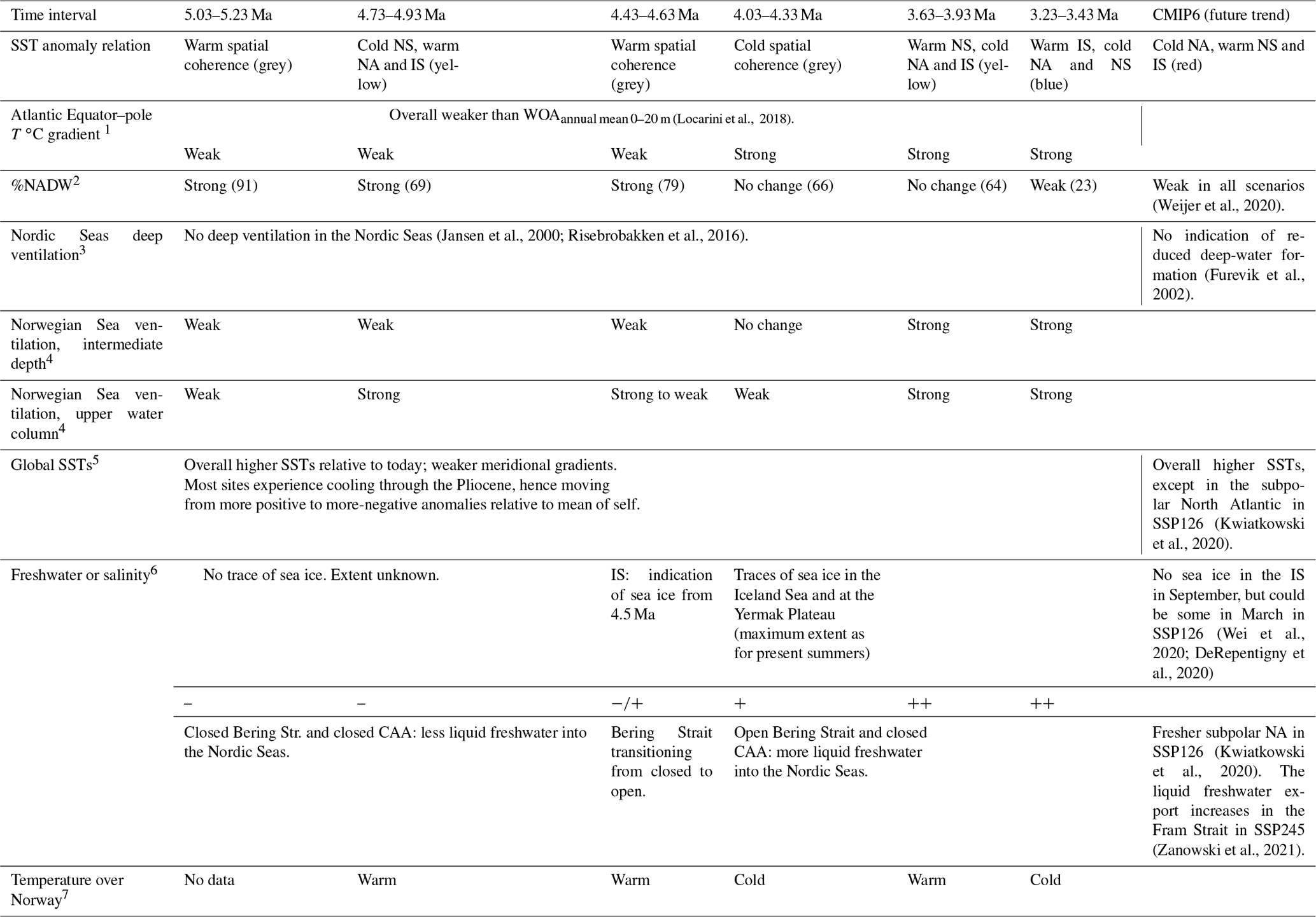
See Fig. S1 in the Supplement. Strength refers to the relative relation between Pliocene states. 2 For Pliocene, the %NADW is calculated following Bell et al. (2015). The indicated strengths are presented relative to Pliocene mean (ca. 62 %NADW). See Fig. S2 and Table S1 in the Supplement for Pliocene background information and dataset references. 3 Not from CMIP6. 4 Ventilation indicated relative to Pliocene mean. For further details, see Fig. S2 in the Supplement. 5 See Figs. S3 and S4 in the Supplement for Pliocene background data. 6 Information about Pliocene sea ice occurrence and extent is extracted from (Clotten et al., 2018; Clotten et al., 2019; Knies et al., 2014). Relative sea ice relation between intervals is indicated by . The references to more or less liquid freshwater refer to a relative relation between Pliocene states. 7 Based on data from Panitz et al. (2018). See Fig. S6 in the Supplement for further information.
We note that minor geographical differences exist between the Pliocene and the present and future. The Greenland Scotland Ridge was deeper by a few hundred metres (Poore et al., 2006), the Canadian Arctic Archipelago was closed (Matthiessen et al., 2009), and the Barents Sea was most likely subaerial (Butt et al., 2002). These differences were, however, constant through the investigated time interval and would therefore not impact the interpretation of our results. In contrast, the Bering Strait opened during the investigated time interval and is suggested to have altered the Arctic freshwater balance and consequently the Nordic Seas oceanography (Table 2) (De Schepper et al., 2015; Otto-Bliesner et al., 2016). The consequences of the opening of the Bering Strait are therefore considered, as the change in freshwater balance will impact the Nordic Seas buoyancy.
The spatial-coherence situation is addressed in Sect. 4.1. The Iceland Sea SST anomaly being different from the North Atlantic and Norwegian Sea SST anomalies is addressed in Sect. 4.2, and the situation when the North Atlantic SST anomaly differs from the SST anomalies of the Iceland and Norwegian seas is addressed in Sect. 4.3. The situation where the Norwegian Sea SST anomaly differs from both the North Atlantic and the Iceland Sea is not seen in any of the idealized experiments. This case will be discussed in Sect. 4.4.
4.1 Spatially coherent SST anomalies
Spatially coherent SST anomalies in the North Atlantic and the Norwegian and Iceland seas are seen at multidecadal timescales in the HadlSST dataset (Fig. 6) and over three Pliocene time intervals covering hundreds of thousands of years, specifically 5.23–5.03, 4.65–4.43, and 4.33–4.03 Ma (Fig. 8). In the observation-based record, the spatial coherence is linked to the continuous northward propagation of heat anomalies from the subpolar region and toward the Arctic, taking about 5–10 years to propagate north, with a frequency of about 14 years (Årthun et al., 2017). Spatially coherent SST anomalies are also seen for more than half of the Pliocene time interval considered in this study, and therefore we also consider spatial coherence to be the norm for Pliocene climate, reflecting the connection of the three regions by ocean circulation (Fig. 1).
From the idealized experiments, spatial coherence is seen under weak freshwater perturbations over the Nordic Seas under constant SATs (Table 1 and Fig. 9b). The responses, however, are small, and none of the selected output parameters from the idealized experiments show responses larger than 2 × SD relative to REF-2 (Table 1). During the cold, spatially coherent interval of the Pliocene, neither the overturning circulation nor the intermediate depth ventilation of the Norwegian Sea deviated from its mean Pliocene conditions (Table 2), consistent with the weak responses seen in the MITgcm experiments for the comparable SST anomaly relation. During the warm, spatially coherent intervals of the Pliocene, the overturning circulation, as derived from the % North Atlantic Deep Water (%NADW) (Table 2), was, however, somewhat stronger than the Pliocene mean, while the intermediate depth ventilation of the Norwegian Sea was weaker than the Pliocene mean (Table 2). In line with a weaker overturning circulation during the cold relative to the warm spatially coherent intervals, a stronger North Atlantic meridional SST gradient and somewhat enhanced freshwater, or buoyancy, forcing characterized the cold relative to the warm spatially coherent SST anomalies of the Pliocene (Table 2). The characteristics associated with the warm, spatially coherent SST intervals are thus less comparable to the MITgcm results than the characteristics associated with the cold, spatially coherent SST interval.
The main difference between the Pliocene periods with warm rather than cold spatially coherent SST anomalies was a somewhat stronger freshwater influence during the cold interval, inferred from the occurrence of the sea ice marker IP25 in the Iceland Sea (Clotten et al., 2019), and that the Bering Strait was fully opened (De Schepper et al., 2015) (Table 2). While there exists evidence for sea ice in the Arctic and the Iceland Sea, it is important to note that the Arctic sea ice extent was considerably smaller than today throughout the Pliocene (Clotten et al., 2019; Knies et al., 2014). Since the Canadian Arctic Archipelago (Fig. 1) was closed throughout the Pliocene (Matthiessen et al., 2009) and since the mean Bering Strait throughflow is directed northward into the Arctic Ocean (Woodgate and Aagaard, 2005), the Fram Strait was the only Arctic Ocean exit during the Pliocene. Opening the Bering Strait allowed for inflow of Pacific water with a lower salinity to the Arctic Ocean and, consequently, enhanced the transport of freshwater from the Arctic Ocean to the Nordic Seas (Hu et al., 2015). Hence, both the increased freshwater influence through the occurrence of sea ice in the Iceland Sea and the open Bering Strait enhanced the Nordic Seas buoyancy. Sensitivity experiments performed with CCSM4 have shown that a closed Canadian Arctic Archipelago entails colder SSTs in the North Atlantic and the Norwegian and Iceland seas relative to the PlioMIP1 experiments, where both the Bering Strait and the Canadian Arctic Archipelago were open (Otto-Bliesner et al., 2016). In the idealized experiments, a weak cold, spatially coherent SST response (less than 2 × SD relative to REF-2) is found with a weak to intermediate freshwater-driven change (P3) in buoyancy. We therefore suggest that the increase in freshwater reaching the Nordic Seas from the Arctic Ocean may have caused the cold, spatially coherent SST anomaly case. We acknowledge that the source and distribution of freshwater is not directly comparable between the Pliocene and the idealized experiments; the freshwater perturbation in the MITgcm experiments is distributed equally over the Nordic Seas basin, while most of the sea ice and liquid freshwater transported from the Arctic Ocean to the Nordic Seas at any time during the Pliocene likely followed the boundary current along the east Greenland margin. The idealized model set-up includes neither the Arctic gateways nor the Arctic sea ice cover. Hence, we stress again that knowledge about changes in the Bering Strait is used to infer changes in the freshwater balance and hence buoyancy in the Nordic Seas, and similarly, the occurrence of more or less sea ice in the Iceland Sea is used to infer the likelihood that a buoyancy change took place. The data from Clotten et al. (2019) show, however, that some of this freshwater also reached the interior Iceland Sea. Less freshwater was available in the region during the Pliocene intervals with warm, spatially coherent SST anomalies, also in line with the idealized experiments where a weak warm, spatially coherent SST response (less than 2 × SD relative to REF-2) is seen for a weak salinity increase (Table 1 and Fig. 9b).
The timescales considered for the observations and the Pliocene reconstructions are very different (multidecadal versus hundreds of thousands of years); however, we consider both to reflect equilibrium, or quasi-equilibrium, responses. The timescales involved in either case are longer than the propagation-driven lag that sets up the spatially non-coherent SST anomaly relation at interannual timescales. Compared to the future scenarios which undergo transient changes due to strong CO2 forcing, we regard the era of instrumental observations to be in quasi-equilibrium. The Pliocene reconstructions represent the predominant situation over hundreds of thousands of years. Higher-frequency variability did take place superimposed on the long-term Pliocene SST variability that we focus on, e.g. exemplified by orbital-scale variability visible in the original raw datasets (Fig. 2). Multidecadal variability is, however, not resolved for any of the relevant Pliocene sites, and the existing age constraints are not good enough to investigate SST anomaly relations at such timescales or even at orbital scales. While not a focus for this study, we note that the amplitude of the Pliocene SST anomalies, from about 1 ∘C to close to 3 ∘C, are larger than the observation-based anomalies that are mostly less than 0.5 ∘C (Fig. 6 and 8).
4.2 An Iceland Sea SST anomaly different from the North Atlantic and the Norwegian Sea
A warm anomaly in the Iceland Sea corresponding with no change in the North Atlantic and the Norwegian Sea is documented for the Pliocene, between 3.43 and 3.23 Ma (Fig. 8). The idealized experiments show that buoyancy changes due to a weak atmospheric warming under constant freshwater forcing (G1 to REF-1 and G2 to REF-3) cause a warm Iceland Sea SST anomaly that differs from the North Atlantic and the Norwegian Seas, where, strictly speaking, no change is seen (Table 1 and Fig. 9a, c). Pliocene air temperatures for the Nordic Seas domain are largely unknown. No information exists from Iceland (Verhoeven et al., 2013). Over Norway, a colder air temperature is indicated between 3.43 and 3.23 Ma, mirroring the colder Norwegian Sea SSTs (Table 2) (Panitz et al., 2018). The data from Panitz et al. (2018) thus suggest a cooling over the Norwegian Sea in contrast to how the idealized experiments result in a warm anomaly in the Iceland Sea corresponding with no change in the North Atlantic and the Norwegian Sea as a response to a weak warming over the full Nordic Seas. Available data therefore cannot confirm that buoyancy change due to warmer atmospheric temperatures over the Nordic Seas may have caused the Iceland Sea SST anomaly to differ from the North Atlantic and the Norwegian Sea.
The idealized experiments that reproduce this warm Iceland Sea and cold North Atlantic and Norwegian Sea SST anomaly relation are associated with a reduction in all the following selected output parameters relative to the respective reference experiment: the density gradient between the northern and southern basin, the velocity of the inflow over the sill, the velocity of the Norwegian Sea boundary current, the heat transport over the sill, and the maximum overturning streamfunction at the sill. Existing Pliocene data indicate a weakened overturning circulation (smaller %NADW contribution) relative to the Pliocene mean between 3.43 and 3.23 Ma (Table 2) despite the Norwegian Sea being well ventilated down to intermediate depths (Risebrobakken et al., 2016) (Table 2). In line with a weakened overturning circulation, a strong Equator-to-pole North Atlantic meridional SST gradient existed due to the relatively cold North Atlantic and Norwegian Sea (Table 2; Fig. S1 in the Supplement). While the Arctic Sea ice cover was still smaller than today (Knies et al., 2014), the constant presence, rather than appearance, of IP25 in the Iceland Sea (Clotten et al., 2018) suggests more available freshwater in the form of spring sea ice relative to the intervals with spatially coherent SST anomalies (Table 2). There was, however, still much less sea ice than today. While not directly comparable, the overall reduction of the overturning at the sill in the idealized experiment seems consistent with a reduced %NADW for this period in the Pliocene (Table 2). The presence of seasonal sea ice, or sea ice transported to the Iceland Sea, suggests a slight freshening and thereby strengthened stratification in the Iceland Sea. Such a change in stratification may lead to reduced dense-water formation and may thereby weaken the NADW formation. The existence of sea ice in the Iceland Sea during the warm Pliocene suggests somewhat enhanced seasonal contrasts. Tests of different model sensitivities and freshwater-forcing scenarios using the Earth system model LOVECLIM have shown that AMOC could be more sensitive to freshwater forcing under warm interglacial climate states with large seasonal contrasts than under warm climate states with a weaker seasonal contrast (Blaschek et al., 2015). However, Blaschek et al. (2015) saw such an AMOC response only when freshwater reached the Labrador Sea convection site and not for future scenarios where less freshwater or sea ice is likely to impact the Labrador Sea. For parts of this Pliocene interval, 3.43–3.23 Ma, some seasonal sea ice existed in the Labrador Sea (Clotten, 2017). Hence, the results of Blaschek et al. (2015) show the same direction in terms of AMOC change as seen in the idealized experiments and from Pliocene data for the warm Iceland Sea and cold North Atlantic and Norwegian Sea SST anomaly relation driven by a buoyancy change due to weak atmosphere warming. A weakened ocean circulation may, again, bring less heat and salt into the Norwegian Sea and, by continuation, the Iceland Sea, further strengthening the stratification.
In the idealized experiments, a non-coherent Iceland Sea SST anomaly scenario is also obtained through strongly increased freshwater-driven buoyancy forcing under constant atmospheric temperatures (P4 to REF-2). However, the resulting response is then a cold SST anomaly in the Iceland Sea and warm anomalies in the North Atlantic and the Norwegian Sea, the opposite situation of what is seen in the Pliocene reconstructions (Figs. 6, 7, and 8).
Hence, from the idealized experiments, we manage to set up a representation of the warm Iceland Sea and cold North Atlantic and Norwegian Sea anomaly scenario. However, the link between the reconstructed background climate and oceanography and the comparable output parameters from the idealized experiments is not straightforward, or relevant data do not exist, emphasizing the need for more data for further evaluation.
4.3 A North Atlantic SST anomaly different from the Norwegian and Iceland seas
A positive SST change (warming) in the Norwegian and Iceland seas corresponding with a small (close to zero) negative SST change (cooling) in the North Atlantic is seen at the end of the century (2068–2098) in CMIP6 future projections, depending on the scenario used (Fig. 7). NorESM2-MM is the least sensitive of the models, and for that model there are still spatially coherent SST anomalies at the end of the century for the SSP126 experiment, showing that the sensitivity of the model plays a role. The SST anomaly relation with the Iceland Sea and Norwegian Sea being different from the North Atlantic found in CMIP6 projections is part of a transient response to an imposed CO2 forcing. Strictly speaking, this case is therefore not representative for an equilibrium or quasi-equilibrium situation, as discussed for all the other SST anomaly relations.
A similar SST anomaly relation, with the North Atlantic being different from the Norwegian and Iceland seas, emerges in the idealized experiments for an intermediate to strong atmospheric warming over the Nordic Seas under constant freshwater (Table 1 and Fig. 9; G2–G4 to REF-1 and G2 to REF-3). Changing the buoyancy by increasing the air temperature over the Nordic Seas reflects what may happen when the atmospheric CO2 concentrations increase in the CMIP6 scenarios; Arctic amplification will entail a larger temperature change over the Nordic Seas than over the North Atlantic.
All these idealized experiments where buoyancy is changed by increasing the air temperature over the Nordic Seas are associated with a reduction in the heat transport over the sill, the maximum overturning streamfunction at the sill, the velocity of the Norwegian Sea boundary current, and the density gradient between the northern and southern basin relative to the respective reference experiments. The AMOC is also weakened compared to the historical level for all CMIP6 scenarios (Weijer et al., 2020) (Table 2). While global SSTs are overall higher for the SSP126 scenario (Table 2), the subpolar North Atlantic cools and freshens (Kwiatkowski et al., 2020). For SSP245, increased export of liquid freshwater is seen in the Fram Strait (Zanowski et al., 2021).
The same SST anomaly relations as found in the CMIP6 future scenario runs were previously identified for CMIP5 future projections (Alexander et al., 2018; Nummelin et al., 2017) and in the Grand Ensemble of the MPI-ESM1.1 climate model (Keil et al., 2020). Keil et al. (2020) show that the heat import to the North Atlantic, associated with a weakening of the low-latitude AMOC, decreases consistently, in parallel with an increased heat transport over the sill set up by a corresponding change in the high-latitude overturning and the subpolar gyre circulation, which is in line with Alexander et al. (2018) and Nummelin et al. (2017). As described above, our idealized experiments show that the SST anomaly relation, with the North Atlantic being different from the other two regions, is associated with a reduced heat transport over the sill, which appears to be opposite to the results from simulated future projections. We stress again that the result from the idealized experiments refers to equilibrium conditions, whereas the CMIP5 and 6 future projections show transient changes to enhanced CO2 forcing and thus have not reached an equilibrium. This is exemplified by the results from Keil et al. (2020), where the ocean heat transport over the sill first increases and then slightly decreases. Therefore, we find it hard to conclude what is causing this SST anomaly relation.
Independent of the exact cause, the indirect effects of both a strong increase in atmospheric CO2 concentrations (CMIP5 and 6 future projections) and increased atmospheric temperatures over the Nordic Seas (idealized experiments) may break the expectation of spatially coherent SST anomalies and set up a non-coherent SST anomaly relation between the North Atlantic (cold) and the Norwegian and Iceland seas (warm).
This SST anomaly relation is not seen during the investigated Pliocene time interval. However, we find it interesting that, despite the large differences in timescales involved (multidecadal versus hundreds of thousands of years), the strongest SST anomaly seen in the future (up to 2 ∘C between 2068 and 2098 for the Norwegian and Iceland seas in CNRM-ESM2-1; Fig. 7) is comparable to the amplitude of the Pliocene SST anomalies (Fig. 8), both of which are larger than the amplitude of the anomalies seen in the instrumental observations (less than 0.8 ∘C; Fig. 6). The amplitude of the future changes depends on both the chosen model and the scenario; these large anomalies are seen for SSP126 in CNRM-ESM2-1 and for SSP585 in NorESM. The CO2 forcing of SSP126 (445 ppm by 2100) is comparable to the high end of the Pliocene CO2 range (427 ppm) (Meinshausen et al., 2020; de la Vega et al., 2020), suggesting that the amplitude of the SST anomalies of the North Atlantic and the Nordic Seas is set by the atmospheric CO2 level and that the response time may be as short as within a century.
4.4 A Norwegian Sea SST anomaly different from the North Atlantic and the Iceland Sea
At two times during the Pliocene, 3.63–3.93 and 4.73–4.93 Ma, the Norwegian Sea SST anomaly differed from both the Iceland Sea and the North Atlantic (Fig. 8). Between 4.73 and 4.93 Ma, a cold SST anomaly was seen in the Norwegian Sea, contemporaneous with a warm anomaly in the Iceland Sea and the North Atlantic. The later period, 3.63 to 3.93 Ma, represents the opposite situation, with a warm Norwegian Sea anomaly corresponding to a cold SST anomaly in the Iceland Sea and the North Atlantic (Fig. 8). None of our idealized experiments resulted in an SST anomaly relation where the Norwegian Sea was different from the other two regions.
During both these Pliocene periods, the %NADW was close to the Pliocene mean strength (Table 2; Fig. S2 in the Supplement). For both cases, the intermediate-depth Norwegian Sea ventilation was stronger than in the periods with spatially coherent SST anomalies and even stronger when the Norwegian Sea was warm relative to the Pliocene mean (Table 2). The main difference between the cold (4.73 to 4.93 Ma) and warm (3.63 to 3.93 Ma) Norwegian Sea anomaly situations was that more freshwater entered the Nordic Seas from the Arctic Ocean in the warm scenario, following the opening of the Bering Strait, and that traces of sea ice were present in the Iceland Sea (Table 2). In addition, the Norwegian Sea intermediate- and upper-water-column ventilation was stronger during the warm-anomaly situation.
Since none of our idealized experiments show this SST anomaly relation, we look further into this case from a conceptual point of view. Two main oceanographic features hold the potential to change the expected spatial coherence at equilibrium between the three locations, namely a change in ocean circulation and advective pathways that weaken the advective interlinkage or a change in water column stratification in one of the regions, e.g. related to an anomalous influx of surface freshwater. A change in the advective pathway could for example be the case if the Iceland Sea is more under the influence of the Irminger Current bringing Atlantic Water to the Iceland Sea directly through the Denmark Strait rather than the water eventually reaching the Iceland Sea via the Norwegian Atlantic Current. A change in the water column stratification, e.g. in the Iceland Sea, may take place if the surface water in the Iceland Sea is more under the influence of the East Greenland Current and thus the polar domain.
Following this conceptual framework, a cold SST anomaly in the Norwegian Sea corresponding to a warm North Atlantic and Iceland Sea SST anomaly may result from a weakened Norwegian Atlantic Current compensated for by a strong Irminger Current. The dominant advective influence of the Nordic Seas is the eastern inflow via the Norwegian Atlantic Current. However, even if anomalies tend to persist throughout the Nordic Seas advective loop, the water that, at the end of this loop, travels south via the Greenland and Iceland seas will qualitatively be cold, as is the case with the water flowing out of the Nordic Seas through the Denmark Strait (e.g. Eldevik et al., 2009; Eldevik and Nilsen, 2013). The Irminger Current, on the other hand, is a warm inflow that directly influences the Iceland Sea, where it largely overturns locally to overflow through the Denmark Strait where it entered (e.g. Våge et al., 2011). A stronger Irminger Current inflow can thus be expected to leave an anomalous warm signature in the Iceland Sea – simply more warm water brought directly into the mix – independent of the anomalous state of the Norwegian Sea and the Norwegian Atlantic Current. Based on existing information, we cannot verify whether or not this was the case between 4.73 and 4.93 Ma.
In contrast, the existence of a warm anomaly in the Norwegian Sea corresponding with cold anomalies in the subpolar North Atlantic and in the Iceland Sea could, in theory, result from a strengthened or expanded East Greenland Current, increasing the fraction of cold polar water reaching the Iceland Sea (Rudels et al., 2005) and the North Atlantic (Dickson et al., 1988). Admittedly, the effect would need to be quite substantial to affect the North Atlantic proper (this is nevertheless what is implied by the common attribution of the hydrographic impact of the great salinity anomaly; Dickson et al., 1988). In general, the state of the subpolar North Atlantic tends to relate more to the larger-scale forcing or subtropical–subpolar-gyre features (e.g. Hátún et al., 2005; Reverdin, 2010), which, in this case, would be aligned to leave the region anomalously cold. The existence of sea ice in the Iceland Sea (Clotten et al., 2019), combined with the effect of enhanced freshwater supply from the Arctic as a response to the fully opened Bering Strait (De Schepper et al., 2015) (Table 2), may lend support to the occurrence of a strengthened or expanded East Greenland Current at the time of a warm Norwegian Sea SST anomaly and cold North Atlantic and Iceland Sea SST anomalies. This interval was quite similar to the cold spatial-coherence situation (Sect. 4.1; Table 2), except that the cold spatial-coherence case was associated with a higher %NADW and weaker ventilation of the upper Norwegian Sea water column. We suggest that changes in the Arctic freshwater balance, and consequently a strengthened East Greenland Current and/or stratification of the Iceland Sea, may be a likely scenario for the cold Iceland Sea and North Atlantic and warm Norwegian Sea anomaly case.
In the MITgcm set-up used, buoyancy is changed by a freshwater change that is evenly spread over the Nordic Seas, and the ocean currents in the interior basin are not very well represented (e.g. the Irminger Current). Combined, this may explain why we do not detect this SST anomaly relation through the idealized experiments. Alternatively, an even-stronger buoyancy change might be needed to set up a similar response for the idealized experiments.
Through our analysis of observation-based data (year 1870 to 2012 AD), CMIP6 projections of the next century, and Pliocene SST reconstructions covering the time interval between 5.23 and 3.13 Ma, we have identified the following four SST anomaly relations between the SSTs of the North Atlantic and the Norwegian and Iceland seas (Fig. 10): (1) spatially coherent SST anomalies (observations and Pliocene – warm and cold spatially coherent anomalies), (2) the Iceland Sea SST anomaly being different from the North Atlantic and the Norwegian Sea (Pliocene – warm Iceland Sea and cold North Atlantic and Norwegian Sea), (3) the North Atlantic SST anomaly being different from the Norwegian and Iceland seas (future scenarios – cold North Atlantic and warm Norwegian and Iceland seas), and (4) the Norwegian Sea SST anomaly being different from the North Atlantic and the Iceland Sea (warm and cold Norwegian Sea corresponding with a cold and warm North Atlantic and Iceland Sea, respectively).
We show that a spatially non-coherent SST anomaly relation can exist in the low-emission (SSP126) and intermediate-emission (SSP585) future scenarios and is not limited to the high-emission scenarios as previously reported. Whether the spatially non-coherent SST anomaly relation is seen in the low-emission scenario or not is, however, dependent on the model's equilibrium climate sensitivity; for the least-sensitive model, NorESM2-MM, the spatially non-coherent SST anomaly relation is not seen in the SSP126 scenario but is seen in the SSP585 scenario. For the SSP126 scenario, the spatially non-coherent SST anomaly is most pronounced in the most sensitive model (CNRM-ESM2-1).
Furthermore, we show that occurrence of spatially non-coherent SST anomaly patterns is not limited to the transient nature of the future scenario runs. Different spatially non-coherent SST anomaly relations occurred during the Pliocene, when the background climate was considered to have been in equilibrium with a CO2 forcing comparable to the present atmospheric concentrations and the SSP126 scenario. While the documented SST anomaly relations take place over a range of different timescales, the SST anomaly relations based on observation and reconstructions, as well as the idealized experiments, represent equilibrium, or quasi-equilibrium, situations. The future change is in that sense the odd case, reflecting a transient response to a given CO2 forcing.
The idealized MITgcm experiments, set up to investigate the impact of buoyancy forcing, reproduce three out of four of the documented SST anomaly relations, emphasizing the key role of buoyancy for setting the northern North Atlantic SST anomalies (Table 1, Figs. 9 and 10). Spatially coherent SST anomalies are seen as a response to weak to intermediate freshwater-induced changes in buoyancy forcing under constant atmospheric temperatures. As the buoyancy forcing, either induced by an SAT or freshwater change, increases, the Iceland Sea SST anomaly becomes different from the North Atlantic and the Norwegian Sea. Under even-stronger buoyancy forcing, the SST anomalies of both the Norwegian and Iceland seas are different from the North Atlantic. Hence, the situation with a warm SST anomaly in the Iceland Sea and cold anomalies in the North Atlantic and Norwegian Sea is the result of a weak atmospheric warming over the Nordic Seas. A stronger atmospheric warming over the Nordic Seas sets up the cold North Atlantic and warm Norwegian and Iceland seas scenario.
Based on the idealized experiments and a literature review of existing Pliocene data, we find that spatially coherent SST anomalies are the norm relative to the mean background climate state under weak buoyancy forcing. The idealized experiments suggest that the situation where the Iceland Sea SST anomaly differs from the Norwegian Sea and the North Atlantic likely reflects a response to a weak increase in atmospheric temperatures under constant freshwater forcing. However, the existing data and data coverage are not good enough to verify this statement. The situation where the North Atlantic SST anomaly differs from the Norwegian and Iceland seas occurs in association with warmer air temperatures caused by increased atmospheric CO2 concentrations.
The case when the Norwegian Sea SST anomaly is different from the North Atlantic and the Iceland Sea, observed for two Pliocene intervals, cannot be explained by the idealized experiments. Here, we suggest that a weakened NwAC compensated for by a strong Irminger Current could, in theory, set up a cold Norwegian Sea anomaly at the same time as the North Atlantic and Iceland Sea experience a warm SST anomaly. The opposite situation, with a warm Norwegian Sea and cold North Atlantic and Iceland Sea SST anomalies, may be linked to an expanded East Greenland Current, increasing the fraction of cold polar water reaching the Iceland Sea. Both more data and further sensitivity studies are needed to settle the discussion on this specific SST anomaly relation.
The amplitude of the SST variability is, overall, larger during the Pliocene than in the observational record. The largest amplitude seen at the end of the 21st century in the Norwegian and Iceland seas is more comparable to the amplitude of the Pliocene SST variability. Why this is the case is out of the scope of this paper and will need to be explored further in future studies. However, since both the Pliocene reconstructions and the future changes occur under atmospheric CO2 concentrations around 400 ppm or higher, these results suggest that the amplitudes of SST anomalies in the Nordic Seas depend on the radiative forcing. Furthermore, the results suggest that, within the timeframe of the future scenarios, SST anomalies can reach amplitudes comparable to the SST anomaly amplitudes seen for Pliocene periods lasting hundreds of thousands of years and in equilibrium with the CO2 forcing, emphasizing how rapidly the Earth system can react to increasing atmospheric CO2 concentrations.
Building on this study, it would be interesting to do similar analyses of the SST anomalies over the investigated region for the last millennia to see if the pattern documented for the observational record holds for a longer historical period with a preindustrial CO2 level. Furthermore, it would be of interest to do a series of sensitivity studies testing the effects of changing the winds over the region, since wind is the other main factor affecting the inflow to the Norwegian Sea. However, the fact that we can explain most of the observed spatial SST patterns emphasizes that buoyancy plays a key role for northern North Atlantic SST variability across the multiple timescales investigated.
All reconstructions are previously published. Information on availability is given in the Supplement.
The observation-based SST dataset from the Met Office Hadley Centre can be accessed from the following link: https://www.metoffice.gov.uk/hadobs/hadisst/ (Met Office Hadley Centre, 2013). We used the HadlSST version 1.1. A detailed description of this dataset is given in Rayner et al. (2003).
Data from the current generation of global climate model simulations are available through the most recent Coupled Model Intercomparison Project Phase 6 (CMIP6) and can be accessed from Earth System Grid Federation (https://esgf-node.llnl.gov/search/cmip6/, WCRP, 2020). We used monthly SST datasets from the CMIP6 ScenarioMIP experiments (O'Neill et al., 2016). All datasets were downloaded through the Analysis Platforms provided by the IS-ENES3 project (https://is.enes.org/sdm-analysis-platforms-service/, is-enes, 2023). The majority of the datasets were download in May–June 2020, and the last years (2095–2100) for MPI-ESM1-2-LR were downloaded in August 2022.
The MITgcm source code (Marshall et al., 1997) is open-source and freely available at https://mitgcm.org (MITgcm, 2023).
The supplement related to this article is available online at: https://doi.org/10.5194/cp-19-1101-2023-supplement.
BR initiated the work, did the Pliocene data analysis, and led the work and the writing. MFJ was responsible for the MITgcm experiments and analyses as well as the writing of the relevant “Data and method” and Results sections. HRL was responsible for the HadlSST and CMIP6 analyses as well as the writing of the relevant “Data and method” and Results sections. TE developed the conceptual explanations and contributed to the MITgcm “Data and method” section. ELM wrote the methodological specifications for the use of alkenones as an SST proxy. All the co-authors were involved in discussions setting the direction of the paper as well as other discussions along the way and have provided input and feedback on the text.
At least one of the (co-)authors is a member of the editorial board of Climate of the Past. The peer-review process was guided by an independent editor, and the authors also have no other competing interests to declare.
Publisher's note: Copernicus Publications remains neutral with regard to jurisdictional claims in published maps and institutional affiliations.
We acknowledge the World Climate Research Programme, which, through its Working Group on Coupled Modelling, coordinated and promoted CMIP6. We thank the climate modelling groups for producing and making available their model output, the Earth System Grid Federation (ESGF) for archiving the data and providing access, and the multiple funding agencies who support CMIP6 and ESGF. We sincerely thank Peipijn Bakker and one anonymous reviewer for their comments that significantly improved the paper.
This research has been supported by the Utdannings- og forskningsdepartementet (through basic funding to the Centre for Climate Dynamics at the Bjerknes Centre for Climate Research). The work builds on results from RCN project nos. 221712 and 229819. The model simulations were performed with resources provided by UNINETT Sigma2 – the National Infrastructure for High-Performance Computing and Data Storage in Norway, project no. NN9709K. The CMIP6 analysis is part of the IS-ENES3 project that has received funding from the European Union's Horizon 2020 research and innovation programme under grant agreement no. 824084.
This paper was edited by David Thornalley and reviewed by Pepijn Bakker and one anonymous referee.
Alexander, M. A., Scott, J. D., Friedland, K. D., Mills, K. E., Nye, J. A., Pershing, A. J., and Thomas, A. C.: Projected sea surface temperatures over the 21st century: Changes in the mean, variability and extremes for large marine ecosystem regions of Northern Oceans, Elem. Sci. Anth., 6, 9, https://doi.org/10.1525/elementa.191 2018.
Årthun, M. and Eldevik, T.: On Anomalous Ocean Heat Transport toward the Arctic and Associated Climate Predictability, J. Climate, 29, 689–704, 2016.
Årthun, M., Eldevik, T., Viste, E., Drange, H., Furevik, T., Johnson, H. L., and Keenlyside, N.: Skilful prediction of northern climate provided by the ocean, Nat. Commun., 8, 15875, https://doi.org/10.1038/ncomms15875, 2017.
Bachem, P., Risebrobakken, B., and McClymont, E. L.: Sea surface temperature variability in the Norwegian Sea during the late Pliocene linked to subpolar gyre and radiative forcing, Earth Planet. Sc. Lett., 446, 113–122, 2016.
Bachem, P. E., Risebrobakken, B., De Schepper, S., and McClymont, E. L.: Highly variable Pliocene sea surface conditions in the Norwegian Sea, Clim. Past, 13, 1153–1168, https://doi.org/10.5194/cp-13-1153-2017, 2017.
Bartoli, G., Hönisch, B., and Zeebe, R. E.: Atmospheric CO2 decline during the Pliocene intensification of Northern Hemisphere glaciations, Paleoceanography, 26, PA4213, https://doi.org/10.1029/2010PA002055, 2011.
Bell, D. B., Jung, S. J. A., Kroon, D., Hodell, D. A., Lourens, L. J., and Raymo, M. E.: Atlantic Deep-water Response to the Early Pliocene Shoaling of the Central American Seaway, Sci. Rep., 5, 12252, https://doi.org/10.1038/srep12252, 2015.
Bendle, J. and Rosell-Melé, A.: Distribution of and in the surface waters and sediments of the Nordic Seas: Implications for paleoceanography, Geochem. Geophy. Geosy., 5, Q11013, https://doi.org/10.1029/2004GC000741, 2004.
Blaschek, M., Bakker, P., and Renssen, H.: The influence of Greenland ice sheet melting on the Atlantic meridional overturning circulation during past and future warm periods: a model study, Clim. Dynam., 44, 2137–2157, https://doi.org/10.1007/s00382-014-2279-1, 2015.
Blindheim, J. and Østerhus, S.: The Nordic Seas, Main Oceanographic Features, in: The Nordic Seas: An integrated Perspective, edited by: Drange, H., Dokken, T., Furevik, T., Gerdes, R., and Berger, W., Geophysical Monograph Series, American Geophysical Union, Washington, DC, 11–38, https://doi.org/10.1029/158GM03, 2005.
Bourke, R. H., Weigel, A. M., and Paquette, R. G.: The Westward Turning Branch of the West Spitsbergen Current, J. Geophys. Res., 93, 14065–14077, 1988.
Bringedal, C., Eldevik, T., Skagseth, Ø., Spall, M., and Østerhus, S.: Structure and forcing of observed exchanges across the Greenland-Scotland Ridge, J. Climate, 31, 9881–9901, https://doi.org/10.1175/JCLI-D-17-0889.1, 2018.
Butt, F. A., Drange, H., Elverhøi, A., Otterå, O. H., and Solheim, A.: Modelling Late Cenozoic isostatic elevation changes in the Barents Sea and their implications for oceanic and climatic regimes: preliminary results, Quaternary Sci. Rev., 21, 1643–1660, 2002.
Clotten, C.: Pliocene Sea Ice Evolution in the Iceland and Labrador Sea – A Biomarker Approach, PhD, Department of Earth Science, Faculty of Mathematics and Natural Sciences, University of Bergen, Bergen, 145 pp., ISBN 978-82-308-3888-4, 2017.
Clotten, C., Stein, R., Fahl, K., and De Schepper, S.: Seasonal sea ice cover during the warm Pliocene: Evidence from the Iceland Srea (ODP Site 907), Earth Planet. Sc. Lett., 481, 61–72, https://doi.org/10.1016/j.epsl.2017.10.011, 2018.
Clotten, C., Stein, R., Fahl, K., Schreck, M., Risebrobakken, B., and De Schepper, S.: On the causes of Sea Ice in the warm Early Pliocene, Sci. Rep., 9, 989, https://doi.org/10.1038/s41598-018-37047-y, 2019.
Conte, M. H., Sicre, M.-A., Rühlemann, C., Weber, J. C., Schulte, S., Schulz-Bull, D. E., and Blanz, T.: Global temperature calibration of the alkenone unsaturation index () in surface waters and comparison with surface sediments, Geochem. Gephy. Geosy., 7, Q02005, https://doi.org/10.1029/2005GC001054, 2006.
de la Vega, E., Chalk, T. B., Wilson, P. A., Bysani, R. P., and Foster, G. L.: Atmospheric CO2 during the Mid-Piacenzian Warm Period and the M2 glaciation, Sci. Rep., 10, 11002, https://doi.org/10.1038/s41598-020-67154-8, 2020.
DeRepentigny, P., Jahn, A., Holland, M. M., and Smith, A.: Arctic sea ice in two configurations of the CESM2 during the 20th and 21st centuries, J. Geophys. Res.-Ocean, 125, e2020JC016133, https://doi.org/10.1029/2020JC016133, 2020.
De Schepper, S., Schreck, M., Beck, K. M., Matthiessen, J., Fahl, K., and Mangerud, G.: Early Pliocene onset of modern Nordic Seas circulation related to ocean gateway changes, Nat. Commun., 6, 8659, https://doi.org/10.1038/ncomms9659, 2015.
Dickson, R. R., Meincke, J., Malmberg, S. A., and Lee, J. A.: The “Great Salinity Anomaly” in the northern North Atlantic 1968–1982, Progress in Oceanography, 20, 103–151, 1988.
Eldevik, T. and Nilsen, J. E. Ø.: The Arctic/Atlantic thermohaline circulation, J. Climate, 26, 8698–8705, https://doi.org/10.1175/JCLI-D-13-00305.1, 2013.
Eldevik, T., Nilsen, J. E. Ø., Iovino, D., Olsson, K. A., Sandø, A. B., and Drange, H.: Observed sources and variability of the Nordic Seas overflow, Nat. Geosci., 2, 406–410, 2009.
Furevik, T., Drange, H., and Sorteberg, A.: Anticipated changes in the Nordic Seas marine climate: Scenarios for 2020, 2050, and 2080, Fisken og Havet, 4, http://hdl.handle.net/11250/113241 (last access: 24 May 2023), 2002.
Furevik, T., Mauritzen, C., and Ingvaldsen, R.: The flow of Atlantic Water to the Nordic Seas and Arctic Ocean, in: Arctic-Alpine Ecosystems and People in a Changing Environment, edited by: Ørbæk, J. B., Kallenborn, R., Tombre, I., Nøst Hegseth, E., Falk-Petersen, S., and Hoel, A. H., Springer, 123–146, https://doi.org/10.1007/978-3-540-48514-8_8, 2007.
Hátún, H., Sandø, A. B., Drange, H., Hansen, B., and Valdimarsson, H.: Influence of the Atlantic Subpolar Gyre on the Thermohaline Circulation, Science, 309, 1841–1844, 2005.
Herbert, T. D., Lawrence, K. T., Tzanova, A., Peterson, L. C., Caballero-Gill, R., and Kelly, C. S.: Late Miocene global cooling and the rise of modern ecosystems, Nat. Geosci., 9, 843–849, 2016.
Holliday, N. P., Hughes, S. L., Bacon, S., Beszczynska-Möller, A., Hansen, A. W., Lavin, H., Loeng, H., Mork, K. A., Østerhus, S., Sherwin, T., and Walczowski, W.: Reversal of the 1960s to1990s freshening trend in the northeast North Atlantic and Nordic Seas, Geophys. Res. Lett., 35, L03614, https://doi.org/10.1029/2007GL032675, 2008.
Hu, A., Meehl, G. A., Han, W., Otto-Bliesner, B., Abe-Ouchi, A., and Rosenbloom, N.: Effects of the Bering Strait closure on AMOC and global climate under different background climates, Prog. Oceanogr., 132, 174–196, https://doi.org/10.1016/j.pocean.2014.02.004, 2015.
IPCC: Climate Change 2021: The Physical Science Basis, in: Contribution of Working Group I to the Sixth Assessment Report of the Intergovernmental Panel on Climate Change, edited by: Masson-Delmotte, V., Zhai, P., Pirani, A., Connors, S. L., Péan, C., Berger, S., Caud, N., Chen, Y., Goldfarb, L., Gomis, M. I., Huang, M., Leitzell, K., Lonnoy, E., Matthews, J. B. R., Maycock, T. K., Waterfield, T., Yelekçi, O., Yu, R., and Zhou, B., Cambridge University Press, Cambridge, UK and New York, NY, USA, 2391 pp., https://doi.org/10.1017/9781009157896, 2021.
is-enes: Analysis Platforms for CMIP6 and CORDEX, https://is.enes.org/sdm-analysis-platforms-service/ (last access: 26 May 2023), 2023.
Jackett, D. R. and McDougall, T. J.: Minimal adjustment of hydrographic profiles to achieve static stability, J. Atmos. Ocean. Tech., 12, 381–389, 1995.
Jansen, E., Fronval, T., Rack, F., and Channell, J. E. T.: Pliocene-Pleistocene ice rafting history and cyclicity in the Nordic Seas during the last 3.5 Myr, Paleoceanography, 15, 709–721, 2000.
Keil, P., Mauritsen, T., Jungclaus, J., Hedemann, C., Olonschenck, D., and Ghosh, R.: Multiple drivers of the North Atlantic warming hole, Nat. Clim. Change, 10, 667–671, 2020.
Knies, J., Cabedo-Sanz, P., Belt, S. T., Baranwal, S., Fietz, S., and Rosell-Melé, A.: The emergence of modern sea ice cover in the Arctic Ocean, Nat. Commun., 5, 5608, https://doi.org/10.1038/ncomms6608, 2014.
Knight, J. R., Allan, R. J., Folland, C. K., Vellinga, M., and Mann, M. E.: A signature of persistent natural thermohaline circulation cycles in observed climate, Geophys. Res. Lett., 32, L20708, https://doi.org/10.1029/2005GL024233, 2005.
Kwiatkowski, L., Torres, O., Bopp, L., Aumont, O., Chamberlain, M., Christian, J. R., Dunne, J. P., Gehlen, M., Ilyina, T., John, J. G., Lenton, A., Li, H., Lovenduski, N. S., Orr, J. C., Palmieri, J., Santana-Falcón, Y., Schwinger, J., Séférian, R., Stock, C. A., Tagliabue, A., Takano, Y., Tjiputra, J., Toyama, K., Tsujino, H., Watanabe, M., Yamamoto, A., Yool, A., and Ziehn, T.: Twenty-first century ocean warming, acidification, deoxygenation, and upper-ocean nutrient and primary production decline from CMIP6 model projections, Biogeosciences, 17, 3439–3470, https://doi.org/10.5194/bg-17-3439-2020, 2020.
Lawrence, K. T., Herbert, T. D., Brown, C. W., Raymo, M., and Haywood, A. M.: High-amplitude variations in North Atlantic sea surface temperature during the early Pliocene warm period, Paleoceanography, 24, PA2218, https://doi.org/10.1029/2008PA001669, 2009.
Lisiecki, L. E. and Raymo, M. E.: A Pliocene-Pleistocene stack of 57 globally distributed benthic δ18O records, Paleoceanography, 20, PA1003, https://doi.org/10.1029/2004PA001071, 2005.
Locarini, R. A., Mishonov, A. V., Baranova, O. K., Boyer, T. P., Zweng, M. M., Garcia, H. E., Reagan, J. R., Seidov, D., Weathers, K., Paver, C. R., and Smolyar, I.: World Ocean Atlas 2018, Volume 1, Temperature, 52, http://www.nodc.noaa.gov/OC5/indprod.html (last access: 20 May 2021), 2018.
Macrander, A., Valdimarsson, H., and Jónsson, S.: Improved transport estimate of the East Icelandic Current 2002–2012, J. Geophys. Res.-Oceans, 119, 3407–3424, https://doi.org/10.1002/2013JC009517, 2014.
Marlowe, I. T., Brassell, S. C., Eglinton, G., and Green, J. C.: Long chain unsaturated ketons and esters in living algae and marien sediments, Ketones, 6, 135–141, 1984.
Marshall, J., Hill, C., Perelman, L., and Adcroft, A.: Hydro-static, quasi-hydrostatic, and non-hydrostatic ocean modeling, J. Geophys. Res., 102, 5733–5752, 1997.
Matthiessen, J., Knies, J., Vogt, C., and Stein, R.: Pliocene paleoceanography of the Arctic Ocean and subarctic seas, Philos. T. R. Soc. A, 367, 21–48, 2009.
Mauritzen, C.: Production of dense overflow waters feeding the North Atlantic across the Greenland-Scotland Ridge. Part 1: Evidence for a revised circulation scheme, Deep-Sea Res. Pt. I, 43, 769–837, 1996.
McClymont, E. L., Ford, H. L., Ho, S. L., Tindall, J. C., Haywood, A. M., Alonso-Garcia, M., Bailey, I., Berke, M. A., Littler, K., Patterson, M. O., Petrick, B., Peterse, F., Ravelo, A. C., Risebrobakken, B., De Schepper, S., Swann, G. E. A., Thirumalai, K., Tierney, J. E., van der Weijst, C., White, S., Abe-Ouchi, A., Baatsen, M. L. J., Brady, E. C., Chan, W.-L., Chandan, D., Feng, R., Guo, C., von der Heydt, A. S., Hunter, S., Li, X., Lohmann, G., Nisancioglu, K. H., Otto-Bliesner, B. L., Peltier, W. R., Stepanek, C., and Zhang, Z.: Lessons from a high-CO2 world: an ocean view from ∼3 million years ago, Clim. Past, 16, 1599–1615, https://doi.org/10.5194/cp-16-1599-2020, 2020.
Meehl, G. A., Senior, C. A., Eyring, V., Flato, G., Lamarque, J.-F., Stouffer, R. J., Taylor, K. E., and Schlund, M.: Context for interpreting equilibrium climate sensitivity and transient climate response from the CMIP6 Earth system models, Science Advances, 6, eaba1981, https://doi.org/10.1126/sciadv.aba1981, 2020.
Meinshausen, M., Nicholls, Z. R. J., Lewis, J., Gidden, M. J., Vogel, E., Freund, M., Beyerle, U., Gessner, C., Nauels, A., Bauer, N., Canadell, J. G., Daniel, J. S., John, A., Krummel, P. B., Luderer, G., Meinshausen, N., Montzka, S. A., Rayner, P. J., Reimann, S., Smith, S. J., van den Berg, M., Velders, G. J. M., Vollmer, M. K., and Wang, R. H. J.: The shared socio-economic pathway (SSP) greenhouse gas concentrations and their extensions to 2500, Geosci. Model Dev., 13, 3571–3605, https://doi.org/10.5194/gmd-13-3571-2020, 2020.
Met Office Hadley Centre: Hadley Centre Sea Ice and Sea Surface Temperature data set (HadISST), Met Office Hadley Centre [data set], https://www.metoffice.gov.uk/hadobs/hadisst/ (last access: May 2013), 2013.
MITgcm: Massachusetts Institute of Technology General Circulation Model, https://mitgcm.org (last access: August 2022), 2023.
Müller, P. J., Kirst, G., Ruhland, G., Vvon Storch, I., and Rosell-Melé, A.: Calibration of the alkenone paleotemperature index based on core tops from the eastern South Atlantic and the global ocean (60∘ N–60∘ S), Geochem. Cosmochem. Ac., 62, 1757–1772, 1998.
Nummelin, A., Li, C., and Hezel, P. J.: Connecting ocean heat transport changes from the midlatitudes to the Arctic Ocean, Geophys. Res. Lett., 44, 1899–1908, https://doi.org/10.1002/2016GL071333, 2017.
O'Neill, B. C., Tebaldi, C., van Vuuren, D. P., Eyring, V., Friedlingstein, P., Hurtt, G., Knutti, R., Kriegler, E., Lamarque, J.-F., Lowe, J., Meehl, G. A., Moss, R., Riahi, K., and Sanderson, B. M.: The Scenario Model Intercomparison Project (ScenarioMIP) for CMIP6, Geosci. Model Dev., 9, 3461–3482, https://doi.org/10.5194/gmd-9-3461-2016, 2016.
Otto-Bliesner, B., Jahn, A., Feng, R., Brady, E. C., Hu, A., and Löfverström, M.: Amplified North Atlantic warming in the late Pliocene by changes in Arctic gateways, Geophys. Res. Lett., 44, 957–964, https://doi.org/10.1002/2016GL071805, 2016.
Paillard, D., Labeyrie, L., and Yiou, P.: Macintosh program performs time-series analysis, EOS T. AGU, 79, 379–379, 1996.
Panitz, S., Salzmann, U., Risebrobakken, B., De Schepper, S., Pound, J. M., Haywood, A., Dolan, A. M., and Lunt, D.: Orbital, tectonic and oceanographic control of Pliocene climate and atmospheric circulation in Arctic Norway, Global Planet. Change, 161, 183–193, 2018.
Poore, H. R., Samworth, R., White, N. J., Jones, S. M., and McCave, I. N.: Neogene overflow of Northern Component Water at the Greenland-Scotland Ridge, Geochem. Geophy. Geosy., 7, Q06010, https://doi.org/10.1029/2005GC001085, 2006.
Prahl, F. G. and Wakeham, S. G.: Calibration of unsaturation patterns in long-chain ketone compositions for paleotemperature assessment, Nature, 330, 367–369, 1987.
Rayner, N. A., Parker, D. E., Horton, E. B., Folland, C. K., Alexander, L. V., Rowell, D. P., Kent, E. C., and Kaplan, A.: Global analyses of sea surface temperature, sea ice, and night marine air temperature since the late nineteenth century, J. Geophys. Res.-Atmos., 108, 4407, https://doi.org/10.1029/2002JD002670, 2003.
Reverdin, G.: North Atlantic subpolar gyre surface variability (1895–2009), J. Climate, 23, 4571–4584, 2010.
Risebrobakken, B., Andersson, C., De Schepper, S., and McClymont, E. L.: Low-frequency Pliocene climate variability in the eastern Nordic Seas, Paleoceanography, 31, 1154–1175, https://doi.org/10.1002/2015PA002918, 2016.
Rosell-Melé, A. and Prahl, F. G.: Seasonality of temperature estimates as inferred from sediment trap data, Quaternary Sci. Rev., 72, 126–136, 2013.
Rudels, B., Björck, G., Nilsson, J., Winsor, P., Lake, I., and Nohr, C.: The interaction between waters from the Arctic Ocean and the Nordic Seas north of Fram Strait and along the East Greenland Current: Results from the Arctic Ocean-02 Oden expedition, J. Mar. Syst., 55, 1–30, 2005.
Ryan, W. B. F., Carbotte, S. M., Coplan, J., O'Hara, S., Melkonian, A., Arko, R., Weissel, R. A., Ferrini, V., Goodwillie, A., Nitsche, F., Bonczkowski, J., and Zemsky, R.: Global Multi-Resolution Topography (GMRT) synthesis data set, Geochem. Gephys. Geosyst., 10, QQ03014, https://doi.org/10.1029/2008GC002332, 2009.
Seidov, D., Baranova, O. K., Biddle, M., Boyer, T. P., Johnson, D. R., Mishonov, A. V., Paver, C., and Zweng, M.: Greenland-Iceland-Norwegian Seas Regional Climatology (NCEI Accession 0112824), NOAA National Centers for Environmental Information [data set], https://doi.org/10.7289/V5GT5K30, 2013.
Seidov, D., Baranova, O. K., Boyer, T. P., Cross, S. L., Mishonov, A. V., Parsons, A. R., Reagan, J. R., and Weathers, K. W.: Greenland-Iceland-Norwegian Seas Regional Climatology version 2, Regional Climatology Team, NOAA/NCEI, https://www.ncei.noaa.gov/products/greenland-iceland-and-norwegian-seas-regional-climatology (last access: 20 May 2021), 2018.
Seland, Ø., Bentsen, M., Olivié, D., Toniazzo, T., Gjermundsen, A., Graff, L. S., Debernard, J. B., Gupta, A. K., He, Y.-C., Kirkevåg, A., Schwinger, J., Tjiputra, J., Aas, K. S., Bethke, I., Fan, Y., Griesfeller, J., Grini, A., Guo, C., Ilicak, M., Karset, I. H. H., Landgren, O., Liakka, J., Moseid, K. O., Nummelin, A., Spensberger, C., Tang, H., Zhang, Z., Heinze, C., Iversen, T., and Schulz, M.: Overview of the Norwegian Earth System Model (NorESM2) and key climate response of CMIP6 DECK, historical, and scenario simulations, Geosci. Model Dev., 13, 6165–6200, https://doi.org/10.5194/gmd-13-6165-2020, 2020.
Smagorinsky, J.: General circulation experiments with the primitive equations: I. The basic experiment, Mon. Weather Rev., 91, 99–164, 1963.
Smedsrud, L. H., Muilwijk, M., Brakstad, A., Madonna, E., Lauvset, S. K., Spensberger, C., Born, A., Eldevik, T., Drange, H., Jeansson, E., Li, C., Olsen, A., Skagseth, O., Slater, D. A., Straneo, F., Våge, K., and Årthun, M.: Nordic Seas Heat Loss, Atlantic Inflow, and Arctic Sea Ice Cover Over the Last Century, Rev. Geophys., 60, e2020RG000725, https://doi.org/10.1029/2020RG000725, 2022.
Spall, M. A.: On the role of eddies and surface forcing in the heat transport and overturning circulation in marginal seas, J. Climate, 24, 4844–4858, https://doi.org/10.1175/2011JCLI4130.1, 2011.
Spall, M. A.: Influences of precipitation on water mass trans-formation and deep convection, J. Phys. Oceanogr., 42, 1684–1700, https://doi.org/10.1175/JPO-D-11-0230.1, 2012.
Talley, L. D., Pickard, G. L., Emery, W. J., and Swift, J. H.: Mass, Salt, and Heat Budgets and Wind Forcing, in: Descriptive Physical Oceanography (Sixth Edition), chap. 5, edited by: Talley, L. D., Pickard, G. L., Emery, W. J., and Swift, J. H., Academic Press, 111–145, https://doi.org/10.1016/C2009-1010-24322-24324, 2011.
Tierney, J. E. and Tingley, M. P.: BAYSLINE: A new calibration for the alkenone paleothermometer, Paleoceanography and Paleoclimatology, 33, 281–301, https://210.1002/2017PA003201, 2018.
Våge, K., Pickart, R. S., Spall, M. A., Valdimarsson, H., Jónsson, S., Torres, D. J., Østerhus, S., and Eldevik, T.: Significant role of the North Icelandic Jet in the formation of Denmark Strait overflow water, Nat. Geosci., 4, 723–727, https://doi.org/10.1038/NGEO1234, 2011.
Verhoeven, K., Louwye, S., and Eiríksson, J.: Plio-Pleistocene landscape and vegetation reconstruction of the coastal area of the Tjörnes Peninsula, Northern Iceland, Boreas, 42, 108–122, 2013.
Wang, K. J., Huang, Y., Majaneva, M., Belt, S. T., Liao, S., Novak, J., Kartzinel, T. R., Herbert, T. D., and Cabedo-Sanz, P. Group 2i Isochrysidales produce characteristic alkenones reflecting sea ice distribution, Nat. Commun., 12, 15, https://doi.org/10.1038/s41467-020-20187-z, 2021.
WCRP: CMIP6, https://esgf-node.llnl.gov/search/cmip6/ (last access: 9 September 2020), 2020.
Wei, T., Yan, Q., Qi, W., Ding, M., and Wang, C.: Projections of Arctic sea ice conditions and shipping routes in the twenty-first century using CMIP6 forcing scenarios, Environ. Res. Lett., 15, 104079, https://doi.org/10.1088/1748-9326/abb2c8, 2020.
Weijer, W., Cheng, W., Garuba, O. A., Hu, A., and Nadiga, B. T.: CMIP6 models predict significant 21st century decline of the Atlantic meridional overturning circulation, Geophys. Res. Lett., 47, e2019GL086075, https://doi.org/10.1029/2019GL086075, 2020.
Woodgate, R. A. and Aagaard, K.: Revising the Bering Strait freshwater flux into the Arctic Ocean, Geophys. Res. Lett., 32, L02602, https://doi.org/10.1029/2004GL021747, 2005.
Zanowski, H., Jahn, A., and Holand, M. M.: Arctic Ocean Freshwater in CMIP6 Ensembles: Declining Sea ice, Increasing Ocean Storage and Export, J. Geophys. Res.-Oceans, 126, e2020JC016930, https://doi.org/10.1029/2020JC016930, 2021.