Atmospheric methane since the last glacial maximum was driven by wetland sources

Atmospheric methane (CH₄) has changed considerably in the time between the last glacial maximum (LGM) and the preindustrial (PI) periods. We investigate these changes in transient experiments with an Earth system model capable of simulating the global methane cycle interactively, focusing on the rapid changes during the deglaciation, especially pronounced in the Bølling–Allerød (BA) and Younger Dryas (YD) periods. We consider all relevant natural sources and sinks of methane and examine the drivers of changes in methane emissions as well as in the atmospheric lifetime of methane. We find that the evolution of atmospheric methane is largely driven by emissions from tropical wetlands, while variations in the methane atmospheric lifetime are small but not negligible. Our model reproduces most changes in atmospheric methane very well, with the exception of the mid-Holocene decrease in methane, although the timing of ice-sheet meltwater fluxes needs to be adjusted slightly in order to exactly reproduce the variations in the BA and YD.

1 Introduction

Between the last glacial maximum (LGM) and the present, the atmospheric concentration of methane (CH₄) changed dramatically. At the LGM, atmospheric CH₄ was at ∼380 ppb (Köhler et al., 2017), whereas it was at 695 ppb at 10 ka; thus, it nearly doubled in concentration during the aforementioned 11 000 years (Fig. 2). Furthermore, the atmospheric concentration changed very rapidly at three points in time: during the transition from the Oldest Dryas into the Bølling–Allerød (BA), during the transition from the BA into the Younger Dryas (YD), and during the transition from the YD to the Preboreal (PB) or Early Holocene. During each of these transitions, atmospheric CH₄ changed by about 150 ppb over a few centuries. Finally, atmospheric methane has more than doubled again between the preindustrial state (1850 CE) and the present (2022 CE). In a previous publication, we investigated the methane emissions during a number of time slices from 20 ka to the present (Kleinen et al., 2020). Time slice investigations, however, are very limited in their explanatory power. They rest on the assumption that the system under investigation is in some kind of an equilibrium state, and they give no information at all on how the system might translate between these states. Therefore, in order to gain insight into highly dynamic changes, transient experiments considering the full dynamics of the system are required. Here, we present the very first transient deglaciation experiments with a state-of-the-art Earth system model (ESM) including a complete methane cycle.

Attempts at modelling methane between the LGM and preindustrial (PI) periods go back several decades and mostly fall into one of two categories. Many of these studies were performed with strongly simplified models, typically box models, that only consider very broad spatial aggregations and an extremely reduced process description, for example Chappellaz et al. (1993), Thompson et al. (1993) and Fischer et al. (2008). The alternative to very simplified models was studies using models with more detailed process descriptions of at least part of the methane cycle, ranging from the wetland emissions of methane to a more or less complete description of the methane cycle, for example Valdes et al. (2005), Weber et al. (2010), Singarayer et al. (2011), Zürcher et al. (2013), Hopcroft et al. (2017) and Kleinen et al. (2020). However, these studies were limited to a few time slices, assuming an equilibrium in climate for these time slices and not covering the trajectories connecting these points in time. Here, we aim to go beyond this state of the art, performing transient experiments with a full ESM specifically adapted to cover the glacial period and the transitions between glacial and interglacial.

The requirements to comprehensively investigate the changes in methane from the LGM to the PI period are demanding. Ice-sheet extent changes by several million square kilometres, sea level changes by about 130 m (Lambeck et al., 2014) and atmospheric CO₂ increases by roughly 50 % (from 180 to 280 ppm) (Petit et al., 1999). These processes, while affecting methane only indirectly, need to be represented in the ESM in order to reproduce the climatic changes driving the changes in the methane cycle. For the methane cycle itself, the global methane budget (Saunois et al., 2016, 2020) considers emissions of fossil fuels as well as agriculture and waste as anthropogenic emissions. These do not need to be considered here, as our experiments mainly consider the time before anthropogenic emissions become relevant. However, emissions from wetlands and wildfires as well as emissions from several other sources lumped into “other natural emissions”, namely termites and wild animals, need to be considered along with the sinks of methane in the atmosphere and soils.

We investigated methane emissions for time slices spaced every 5000 years, starting at the LGM and ending at the present, in Kleinen et al. (2020). We also showed the evolution of atmospheric CH₄ for the next millennium under a number of scenarios in Kleinen et al. (2021). In the present publication, we bring these two together and investigate the transient evolution of the methane cycle from the LGM to the PI period, mainly focusing on the period with the largest changes in climate and methane from 18 to 10 ka which includes the fast and massive changes during the Bølling–Allerød and Younger Dryas.

2 Modelling the methane cycle in the Max Planck Institute for Meteorology Earth System Model (MPI-ESM 1.2)

2.1 MPI-ESM 1.2 in transient deglaciation experiments

We use MPI-ESM, the Max Planck Institute for Meteorology Earth System Model (Mauritsen et al., 2019; Mikolajewicz et al., 2018), consisting of the ECHAM6 atmospheric general circulation model, the MPI-OM ocean general circulation model, and the JSBACH land surface model in coarse resolution (T31GR30 ≈ $\mathrm{3.75}{}^{\circ }\times \mathrm{3.75}{}^{\circ }$), to investigate the evolution of atmospheric methane during the deglaciation. The basis for our modelling set-up is model version 1.2, which is the same model version used in the Coupled Model Intercomparison Project Phase 6 (CMIP6; Eyring et al., 2016).

MPI-ESM, similar to many other ESMs, considers the land–sea and glacier masks as well as the river routing as fixed. To determine the transient evolution of climate, these are updated automatically in our model version, as described in Meccia and Mikolajewicz (2018) and Riddick et al. (2018). Briefly, the model evaluates the changes in ice sheet and sea level after every decade. From these, combined with the RTopo-2 topography (Schaffer et al., 2016), it determines a new land–sea mask, bathymetry and orography as well as a new river routing set-up to be used for the next decade in the model experiment.

2.2 Modelling the methane cycle

Based on the recent Global Carbon Project CH₄ budget (Saunois et al., 2016, 2020), we consider methane emissions from wetlands, termites, wildfires and herbivores as relevant during the deglaciation, and we also include emissions from geological sources. We assume the latter to be independent of climate and, therefore, prescribe them, whereas we aim to model all of the former interactively. We neglect anthropogenic methane emissions in the experiments described here, as they are highly uncertain but likely very small for the time period considered here. In terms of methane sinks, the atmospheric sink of methane is most important, and soils are a secondary sink. We include both of them in our model.

2.2.1 Methane emissions from wetlands, termites, wildfires and geological sources

The basic methane emission model for emissions from wetlands, termites and wildfires is described in Kleinen et al. (2020); thus, we cover it only briefly here. We use a TOPMODEL (Beven and Kirkby, 1979) approach to determine inundated areas; we then determine the wetland methane emissions in these areas based on the model by Riley et al. (2011). Methane emissions from fires are determined using the SPITFIRE fire model (Lasslop et al., 2014), employing emission factors by Kaiser et al. (2012). Termite methane emissions are estimated using the approach from Kirschke et al. (2013) and Saunois et al. (2016).

In the TOPMODEL approach (Beven and Kirkby, 1979), we combine the soil water content determined in the MPI-ESM land surface model JSBACH with sub-grid-scale topographic information, the compound topographic index (CTI), in order to determine the variation in the water table in each model grid cell. For our experiments, we use the CTI index product by Marthews et al. (2015) for the present-day land areas and combine it with CTI index values that we derived from the ETOPO1 dataset (Amante and Eakins, 2009) for those areas that are below sea level at present, using the TOPMODEL R library (Buytaert, 2011). We then use the variation in water table to determine the inundation fraction: the fraction of each grid cell where the water table is at or above the surface. In Kleinen et al. (2020), we evaluated the model for present-day climatic conditions against remote-sensing data of inundation (Prigent et al., 2012). Total extent and seasonality are similar for the Northern Hemisphere (NH) extratropics, while the model slightly overestimates the extent for tropical inundation. Thus, we assess the agreement between the model and data as being reasonable, considering the limitations of both the model and the remote-sensing data.

In JSBACH, the YASSO model (Goll et al., 2015) is used to determine the decomposition of soil carbon. In the inundated areas, we assume anaerobic decomposition, with decomposition rate constants reduced to 35 % of the YASSO values used for aerobic decomposition, as proposed by Wania et al. (2010). The anaerobic decomposition of carbon produces both CO₂ and CH₄, with a temperature-dependent partitioning into the two decomposition products as described by Riley et al. (2011). The transport of O₂, CO₂ and CH₄ is determined in a methane emission model based on Riley et al. (2011), which explicitly simulates the methane transport via the diffusion, ebullition and plant aerenchyma pathways. The oxidation of CH₄, if sufficient oxygen is present, is considered as well, following Michaelis–Menten kinetics. Furthermore, the transport model also determines the soil sink of methane, as CH₄ diffuses into the soil in areas where little methane is produced (i.e. in dry areas) and is subsequently oxidised.

Lake methane emissions are not modelled explicitly; rather, we assume that their emissions are implicitly contained in the wetland flux. We make this simplification for pragmatic reasons, as we have not found an appropriate model for lake areas under changing climatic conditions in the literature. We assume, however, that the error introduced by this simplification is relatively minor on the scales that the model was designed for (an approximate >350 km spatial resolution and a decadal to centennial temporal scale). We base this assumption on two factors. First, we used surface water extent data to calibrate the wetland model, and these data also contain inland waterbodies. Second, we assume that the changes in methane fluxes from inland waters on these scales will be driven by the same factors that drive the changes in wetland emissions, i.e. soil carbon content, temperature and precipitation. However, on shorter temporal (monthly to annual) and spatial (10s of kilometres) scales, the errors introduced through this simplification may be significant.

Methane emissions from wildfires and biomass burning (with the sum subsequently called “fire” emissions) are determined from the SPITFIRE fire model (Lasslop et al., 2014) using emission factors from Kaiser et al. (2012). The SPITFIRE fire model determines the spread of fires using the fire ignition probability, which is a function of lightning frequency and population density (assuming negligible human impact on fires before 12 ka due to a small population size and using Klein Goldewijk et al., 2017, afterwards); flammability (higher under dryer and warmer conditions); and the amount of biomass available for burning. The methane emissions are then determined from the burned biomass using emission factors. Termite methane emissions are estimated using the approach by Kirschke et al. (2013) and Saunois et al. (2016), which determines termite mass from gross primary productivity in tropical areas and assumes a constant emission factor to determine the final methane emissions. Finally, methane emissions from geological sources are prescribed using a spatial distribution from Etiope (2015), although they are scaled down to give total geological methane emissions of 5 Tg CH₄ yr⁻¹, as Petrenko et al. (2017) and Hmiel et al. (2020) showed (from ice-core data) that geological emissions larger than this value are not possible for either the Younger Dryas or the PI period.

In Kleinen et al. (2020), we evaluated the modelled methane emissions for the present-day (PD) climate. As flux measurements on appropriate scales are not available, we compared aggregate fluxes against global assessments (Saunois et al., 2016). We found that the model simulates wetland methane emissions of 222 Tg CH₄ yr⁻¹ (decadal mean over 2000–2009), reduced to 190 Tg CH₄ yr⁻¹ in this study as detailed below; fire emissions of 17.6 Tg CH₄ yr⁻¹; termite emissions of 11.7 Tg CH₄ yr⁻¹; and a soil uptake of 17.5 Tg CH₄ yr⁻¹. These values fall well within the ranges reported by Saunois et al. (2016), who reported 153–227 Tg CH₄ yr⁻¹ for natural wetlands, 15–20 Tg CH₄ yr⁻¹ for biomass burning, 1–5 Tg CH₄ yr⁻¹ for wildfires, 3–15 Tg CH₄ yr⁻¹ for termites and 9–47 Tg CH₄ yr⁻¹ for the soil uptake. Spatial patterns of PD emissions are also similar to those shown by Saunois et al. (2016). Furthermore, wetland methane emission estimates from atmospheric inversions (Bousquet et al., 2011) show that the majority (62 %–77 %) of the PD emissions comes from regions between 30^∘ S and 30^∘ N, while a much smaller part (20 %–33 %) is emitted north of 30^∘ N. Of the modelled total wetland CH₄ emissions for PD conditions, 70 % of the emissions are from low-latitude regions, while 29 % of the emissions are from regions north of 30^∘ N. Therefore, the latitudinal distribution of modelled PD wetland methane emissions is well within the range obtained from atmospheric inversions.

In order to accommodate the additional methane flux from the consideration of herbivorous mammals in the present publication, we recalibrated the wetland emission model in comparison with Kleinen et al. (2020), reducing wetland emissions to 190 Tg CH₄ yr⁻¹ for the 2000–2009 CE decadal mean, thereby keeping total emissions for the present day roughly constant, despite the additional consideration of herbivore emissions.

2.2.2 Methane emissions from herbivores

At present, emissions from herbivores, especially cows, make up a significant part of the methane emissions (Saunois et al., 2020). This fact is, however, the result of human action, as it has to be assumed that the number of ruminants was significantly smaller before humans began herding cows. Previous approaches to estimate the methane emissions from herbivores (Crutzen et al., 1986; Chappellaz et al., 1993; Hristov, 2012; Smith et al., 2016) generally start from the level of individual animals, relating methane emissions to species and body mass. They then rely on estimates of population numbers for specific species to determine total emissions from herbivores. In order to apply such an approach in the context of an Earth system model and past climate states, one would need to somehow relate population densities of certain species via vegetation productivity to climate; however, we found this impossible due to a lack of data, especially for ecosystems untouched by humans, as these no longer exist. Furthermore, a recent review of methane production by mammalian herbivores (Clauss et al., 2020) found that CH₄ yields (CH₄ production per unit dry matter, DM, intake) do not vary significantly with body mass nor between ruminants and non-ruminants, thereby negating two of the foundations of the previous approaches to estimating herbivore methane emissions. Instead, they found that absolute CH₄ emissions scaled linearly with DM intake, which allows for a simplified treatment of herbivore methane emissions in our model.

As part of the carbon cycle representation, the JSBACH model determines a carbon flux from herbivory, F_herbivory (Schneck et al., 2013; Reick et al., 2021). Here, $F_{\mathrm{herbivory}}=r_{\mathrm{herbivory}}\times C_{\mathrm{G}}$, where r_herbivory is a constant dependent on the plant functional type and C_G is the carbon content in the “green” carbon pool, i.e. the carbon pool representing the living parts of plants (leaves, fine roots and vascular tissues). We further assume that a fraction of the herbivory flux is consumed by mammals, f_mammal; f_mammal=0.016 in forest and f_mammal=0.32 in grasslands. These latter values were chosen ad hoc but seem plausible. Finally, we use a CH₄ yield γ of γ=14.9 g(CH₄) kg(DM)⁻¹, obtained as a mean over the values for all species listed in Clauss et al. (2020). Thus, the final CH₄ flux from herbivory, $H_{{\mathrm{CH}}_{\mathrm{4}}}$, is as follows:

$$\begin{array}{}\text{(1)}& H_{{\mathrm{CH}}_{\mathrm{4}}}=f_{\mathrm{mammal}}\times \mathit{\gamma }\times F_{\mathrm{herbivory}}.\end{array}$$

2.3 Atmospheric methane sink

As described in Kleinen et al. (2021), the spatiotemporal evolution of the methane abundance in the ECHAM6 atmospheric model is simulated using a methane tracer which undergoes transport and chemical removal, while emissions are calculated using the JSBACH land surface model. The atmospheric sink of methane is calculated using a zonally averaged reactivity field obtained from the comprehensive ECHAM/MESSy Atmospheric Chemistry (EMAC) model (Joeckel et al., 2010). This reactivity field contains, in aggregated form, all atmospheric sink terms considered in the EMAC model (i.e. reaction with OH, tropospheric Cl, stratospheric reactions, etc.).

Following Gromov et al. (2018) and Kleinen et al. (2021), the subsequent updated parameterisation is used to account for variations in the atmospheric oxidative capacity and, therefore, tropospheric CH₄ reactivity $r_{{\mathrm{CH}}_{\mathrm{4}}}$:

$$\begin{array}{}\text{(2)}& r_{{\mathrm{CH}}_{\mathrm{4}}}=\mathit{\alpha }\times {\left(\mathrm{LN}+k_{\mathrm{N}}\mathrm{RN}\right)}^p\times {\left(M+k_{\mathrm{C}}\mathrm{RC}+k_{\mathrm{A}}A\right)}^q\left[{\mathrm{yr}}^{-\mathrm{1}}\right],\end{array}$$

where LN is the global emission of lightning nitrogen oxides (NO_x), simulated interactively according to Price and Rind (1992, 1993); M is the CH₄ atmospheric burden; RN and RC are the terrestrial (surface) emissions of reactive nitrogen (NO_x) and carbon compounds given in Tg N yr⁻¹ and Tg C yr⁻¹ for the emission fluxes, respectively; and A is the mean tropospheric reactive aerosol surface area (about 100 Mm² in both present-day and past climates). Fit parameters (α=7.45 Tg N^−p Tg C^−q yr⁻¹, p=0.36, $q=-\mathrm{0.60}$, k_N=0.59, k_C=4.25 and k_A=4.21 Tg C Mm⁻²) are obtained from an ensemble of EMAC simulations covering a broad range of RN, RC, LN and M values under LGM (21 ka), Middle Holocene (6 ka), PI and PD conditions. The fitted $r_{{\mathrm{CH}}_{\mathrm{4}}}$ value is accurate to 7 % at 95 % confidence intervals (CIs). In the MPI-ESM experiments, the natural emission components of RN and RC are obtained from the Model of Emissions of Gases and Aerosols from Nature (MEGAN) model (Guenther et al., 2012) for the biogenic sources and from the SPITFIRE model (Lasslop et al., 2014), with emission factors from Kaiser et al. (2012), for fire emissions. We use the terrestrial NO_x emissions for the RN term, and we use the biogenic CO and isoprene (C₅H₈) fluxes, scaled by a factor of 1.4 to account for secondary biogenic co-emitted compounds, as proxies for the total RC emitted. These scaling factors were derived from the simulated PD total RC emissions. In experiments covering the historical and future periods, anthropogenic emissions of RC and RN would be considered as well (see Kleinen et al., 2021), but they are neglected for the experiments described below.

2.4 Model forcing and experiments

We forced the model with prescribed orbital parameters from Berger (1978) and greenhouses gases from Köhler et al. (2017). Orbital parameters and greenhouse gas concentrations are supplied to the model as decadal means and are updated every 10 model years. Atmospheric aerosols were prescribed to constant 1850 CE conditions (Kinne et al., 2013), and we considered no anthropogenic land use. Ice-sheet extent was prescribed from the GLAC-1D ice-sheet reconstruction (Tarasov et al., 2012; Briggs et al., 2014; Ivanovic et al., 2016). Ice-sheet extent, bathymetry and topography (Meccia and Mikolajewicz, 2018), and river routing (Riddick et al., 2018) were continuously updated every 10 model years.

We initialised the model from a spin-up experiment at constant 26 ka boundary conditions, running for several millennia. From this model state, we performed a transient model experiment until PI times, with continuously updated ice-sheet extent, bathymetry, topography and river routing, similar to the experiments described by Kapsch et al. (2022). In this experiment, called “base” in the following, the prescribed ice-sheet forcing from the GLAC-1D reconstruction leads to a collapse of the Atlantic Meridional Overturning Circulation (AMOC) early in the Bølling–Allerød (Kapsch et al., 2022), due to excess meltwater entering the North Atlantic, and the Younger Dryas does not occur in this experiment. Thus, we performed a second experiment, called “MWM” (meltwater manipulation), in which we manipulate the meltwater fluxes from the Laurentide ice sheet: starting in 15.2 ka, we prevent meltwater from the Laurentide ice sheet from reaching the ocean, instead storing it. We then release this accumulated meltwater over a period of 1200 years, starting in 12.8 ka, adding it to the Mackenzie River watershed, thereby mimicking the storage of glacial meltwater in proglacial lakes, like Lake Agassiz, and its subsequent release (Murton et al., 2010).

3 Results

3.1 Transient climate and land carbon changes

At the last glacial maximum, around 20 ka, the global mean temperature is 282 K in our model, which is 4.7 K lower than during the PI period (Fig. 1a). As the ice sheets melt and CO₂ increases, the temperature begins to rise significantly after 18 ka, with the rate of temperature increase declining after 9 ka. Dallmeyer et al. (2022) evaluated model temperatures in the experiment against reconstructions and found a reasonably close match, as illustrated by the comparison against the reconstructions by Shakun et al. (2012) and Osman et al. (2021) in Fig. 1a. While Shakun et al. (2012) reconstructed a smaller temperature change between the LGM and the Holocene than we see in our experiments, Osman et al. (2021) reconstructed a larger temperature change, with our experiment situated between the two. The AMOC (Fig. 1b) is relatively stable at about 20 Sv between the LGM and 14.8 ka. Here, the base and MWM experiments diverge: in the base experiment, meltwater pulse (MWP) 1a, a sea level rise event recorded in Barbados corals (Fairbanks, 1989), leads to a strong freshening of the North Atlantic and a near-complete AMOC shutdown (remaining overturning of 1 Sv) at 14.38 ka, which in turn leads to a drop in global mean temperature by nearly 1 K. Nevertheless, temperature and the AMOC recover quickly. The AMOC continues to be highly variable until 9 ka, with a further near collapse from MWP 1b at 11.4 ka. Global mean temperature, however, is affected significantly less by the AMOC reduction at MWP 1b than at MWP 1a. After 9 ka, the AMOC is relatively stable, although at a slightly smaller overturning of 18.7 Sv (during the PI period). Similar to global mean temperature, the total land carbon stock (Fig. 1c) remains nearly constant at 970 Pg C, which is 718 Pg C less than during the PI period, from the LGM to 18 ka. Subsequently, total land C increases until 10.95 ka. Afterwards, only minor changes in total land carbon stock occur until the PI state, with a total land C stock of 1688 Pg C. The AMOC collapse at 14.38 ka caused by MWP 1a leads to a short decrease in the C stock of about 6.8 %, but the total duration of this excursion is about 800 years and carbon continues to rise after it.

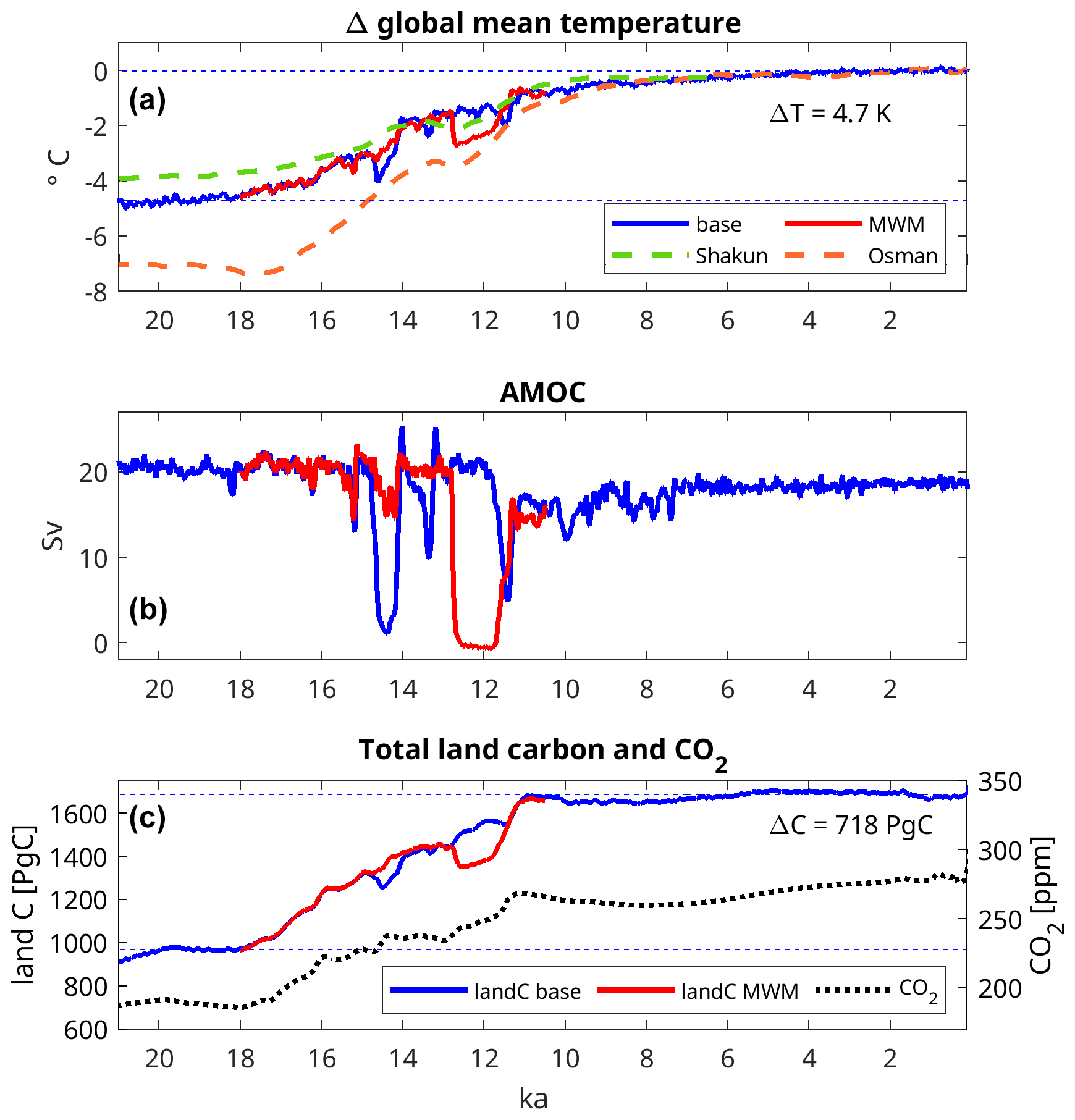
Figure 1 Overview of climatic and land carbon changes from the LGM to the PI period: (a) global mean temperature change, (b) North Atlantic meridional overturning circulation, and (c) total land carbon storage and atmospheric CO₂. The base experiment is shown in blue, and the MWM experiment is shown in red. Panel (a) also contains the temperature change reconstructed by Shakun et al. (2012) and Osman et al. (2021), while the reconstructed atmospheric CO₂ in panel (c) is from Köhler et al. (2017).

In the MWM experiment, the initial collapse of the AMOC at 14.38 ka is prevented by the manipulation of the meltwater fluxes, and temperature and carbon continue to rise during this period. As we release the accumulated Laurentide ice-sheet meltwater at 12.8 ka, the AMOC collapses, with the consequence of a 1.25 K drop in global mean temperature and a 100 Pg C or 6.9 % decrease in the terrestrial C stock. After we end the meltwater manipulation in 11.6 ka, temperature, the AMOC and land carbon stocks recover quickly.

3.2 Transient changes in methane

In comparison to a stack of ice-core-derived CH₄ concentrations in Antarctica (Köhler et al., 2017), the atmospheric concentration of methane in our experiments is quite reasonable overall (Fig. 2a), although there are significant discrepancies during some periods. In the ice core, methane is nearly constant at ∼370 ppb from the LGM to 18 ka, at which point it starts increasing slowly. At 14.6 ka (the transition into the Bølling–Allerød warm period), CH₄ increases abruptly by ∼150 ppb, decreasing again at 12.8 ka (the transition into the Younger Dryas). At the end of the YD, at about 11.5 ka, CH₄ again increases abruptly and stays roughly constant at ∼690 ppb for the next 2000 years. Finally, ice-core CH₄ slowly decreases by ∼120 ppb during the Early Holocene between 9 and 4.5 ka, recovering after the Middle Holocene to ∼690 ppb during the PI period.

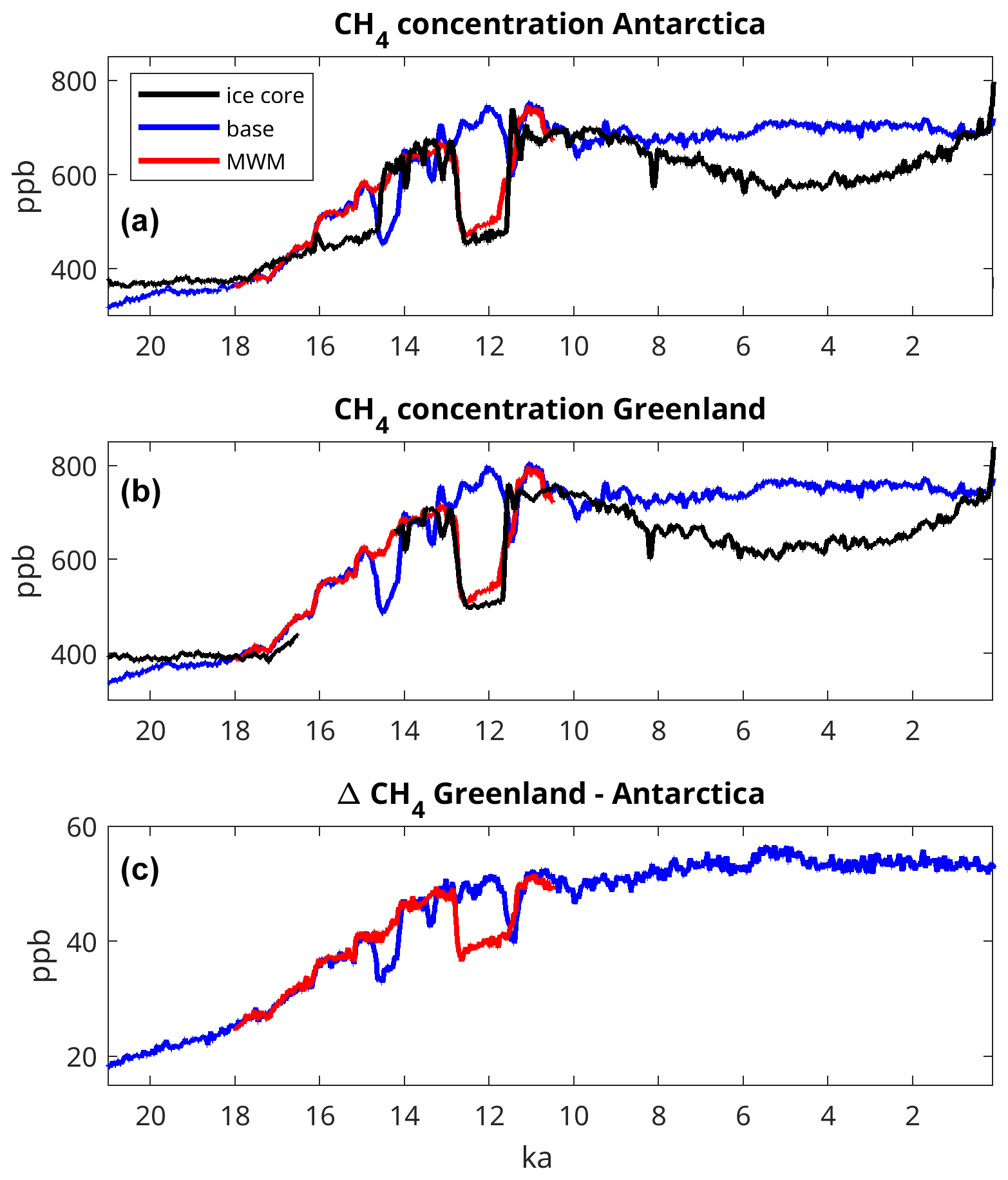
Figure 2 Atmospheric concentration of CH₄ over (a) Antarctica and (b) Greenland in the MPI-ESM base and MWM experiments as well as in ice-core data. Antarctic ice-core data are from Köhler et al. (2017), and Greenland ice-core data are from Chappellaz et al. (2013) and Beck et al. (2018). (c) Interpolar gradient of atmospheric CH₄, expressed as the difference in the CH₄ concentration between Greenland and Antarctica.

Modelled atmospheric CH₄ over Antarctica is only slightly lower than reconstructed at 20 ka (370 ppb in the ice core and 350 ppb in the model; Table 1), although the discrepancy is larger at 21 ka. Similar to reconstructions, the atmospheric CH₄ starts rising significantly at 18 ka, but the increase at the beginning of the Bølling–Allerød and the drop in methane during the transition into the Younger Dryas are dissimilar, at least in the base experiment: in terms of atmospheric CH₄, the Bølling–Allerød seems to start earlier, at 16 ka instead of 14.6 ka. At 14.38 ka, near the beginning of the BA in reconstructions, the base experiment displays a significant drop in atmospheric methane, caused by the AMOC shutdown after MWP 1a. For the transition into the Younger Dryas at 12.8 ka, on the other hand, the base experiment continues at high levels of atmospheric methane and does not show the decrease in methane displayed by the ice-core data, as the model shows no climatic transition at this time.

Table 1 Simulated and reconstructed CH₄ concentrations (ppb) at the ice-core sites for selected time periods.

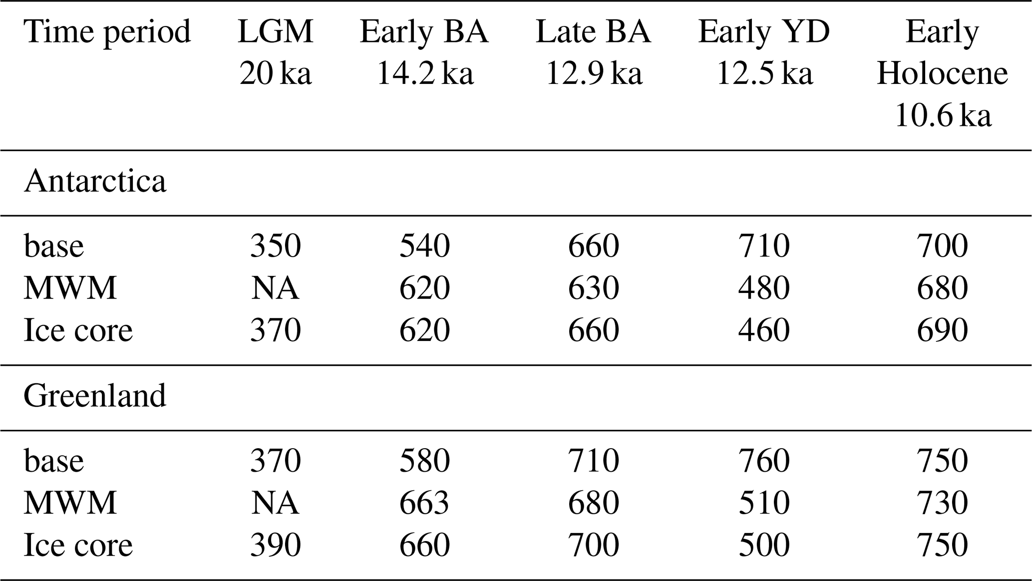
NA stands for not available.

The MWM experiment differs from the base experiment at the beginning of the Bølling–Allerød, as the atmospheric concentration of methane does not change at the beginning of the BA. Instead, it is very similar to the ice-core data. Furthermore, the atmospheric concentration of methane very rapidly decreases by 25 % at the beginning of the Younger Dryas at 12.8 ka, similar to ice-core data (−29 %). At the end of the Younger Dryas, recovery of atmospheric methane occurs slightly earlier than in the ice-core data, although not as quickly. Therefore, the Younger Dryas in our MWM experiment is quite similar to the ice-core data. For atmospheric methane during the Holocene, however, there is a significant divergence between model results and ice-core data: while ice-core CH₄ slowly decreases towards the mid-Holocene and increases again during the Late Holocene, the model results show constant atmospheric CH₄ throughout the Holocene.

A comparison to Greenland ice cores is much more intricate, as recent investigations show excess CH₄ in some Greenland ice-core records (Lee et al., 2020). This issue has not yet been resolved fully; thus, we do not show a full ice-core CH₄ time series from Greenland. Instead, we focus on data derived from the NEEM (North Greenland Eemian Ice Drilling) ice core (Chappellaz et al., 2013), which were obtained using a continuous-flow measurement technique and are, thus, presumably less susceptible to the generation of excess CH₄, as well as data from the Holocene (Beck et al., 2018), when the dust concentration was much lower. For those times when data are available (earlier than 17.5 ka and 14 ka to the PI period), the comparison for Greenland (Fig. 2b) is of a similar quality to the comparison for Antarctica. Thus, Greenland CH₄ is very similar for 20–18 ka, and the evolution of methane during the Bølling–Allerød to Younger Dryas transition is also very similar in model and ice-core data if one considers the MWM experiment (Table 1). Therefore, our model captures the gradient in methane between Greenland and Antarctica adequately for key periods of the deglaciation. The interpolar gradient, shown here as the difference in the atmospheric CH₄ concentration between Greenland and Antarctica (Fig. 2c) is positive throughout the experiment, with values at the LGM near 20 ppb and PI values of about 55 ppb. Again, the rate of increase is highest between 18 and 10.5 ka, with relatively stable values throughout the Holocene. Finally, the tropical methane concentration (Fig. A1a) remains in between the values for Antarctica and Greenland throughout the experiment, which is in contrast to previous studies that have shown the highest LGM methane concentrations in the tropics (Valdes et al., 2005).

The terrestrial methane fluxes (Fig. 3) largely determine the atmospheric methane concentration. The net CH₄ flux (Fig. 3a) increases from 90 Tg CH₄ yr⁻¹ at 20 ka to 165 Tg CH₄ yr⁻¹ during the PI period, with emissions staying very similar between 20 and 18 ka, increasing more strongly between 18 and 11 ka, and staying nearly constant between 10 ka and the PI period. In the base experiment, emissions decrease strongly as a response to the AMOC collapse after MWP 1a, with emissions recovering quickly as the AMOC resumes, which is a pattern that continued after MWP 1b. In the MWM experiment, however, we see a 32 Tg CH₄ yr⁻¹ reduction in net emissions in response to the AMOC collapse induced by the meltwater manipulation, followed by a quick recovery as the manipulation ceases. Wetland fluxes (Fig. 3b) are the most important component of the net CH₄ flux; thus, their temporal change is rather similar to the net flux, although at a slightly smaller overall magnitude, with wetland emissions of 79 Tg CH₄ yr⁻¹ at 20 ka and 142 Tg CH₄ yr⁻¹ during the PI period, while the emission reduction from the AMOC collapse in the MWM experiment is 32 Tg CH₄ yr⁻¹. Here, the AMOC collapse leads to a significant decrease in NH temperatures around the Atlantic Ocean, in turn leading to decreased evaporation and, thus, decreased precipitation, thereby decreasing wetland areas and methane production in the NH tropics. The non-wetland methane fluxes (Fig. 3c) are of significantly smaller magnitude than the wetland fluxes, with emissions at 20 ka of 7.4 Tg CH₄ yr⁻¹ for herbivores, 2.8 Tg CH₄ yr⁻¹ for termites, 3.2 Tg CH₄ yr⁻¹ for fire emissions and −2.2 Tg CH₄ yr⁻¹ for the methane uptake in upland soils. Towards the PI state, these fluxes increase to 14.5, 6.3, 10.9 and −6.3 Tg CH₄ yr⁻¹ for herbivores, termites, fires and uptake, respectively. Here, the differences between the base and MWM experiments are small; thus, we omit the MWM experiment from Fig. 3c. The dynamics of the uptake flux appear to be different from the other fluxes at first glance, with pronounced differences for the Bølling–Allerød and Younger Dryas at the same times as they appear in proxy records. This is due to the fact that the most important driver of terrestrial methane uptake is the atmospheric concentration of methane (Kleinen et al., 2020), which we prescribed from ice-core data for the uptake flux.

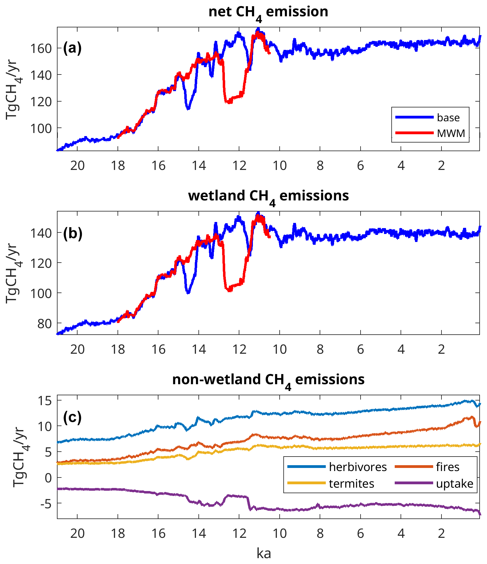
Figure 3 Terrestrial methane in the MPI-ESM base and MWM experiments: (a) net flux, (b) wetland emission flux, and (c) non-wetland methane emissions from herbivores, fires, termites and terrestrial methane uptake.

We model the atmospheric sink of methane as a function of terrestrial emissions of reactive carbon (RC) as well as the NO_x emissions from the soil/vegetation and lightning (Eq. 2). The temporal changes in RC emissions during the deglaciation (Fig. 4a) are very similar to the changes in CH₄ emissions: at 20 ka, RC emissions are 270 Tg C yr⁻¹, and they start increasing noticeably at 18 ka, reaching a maximum of 500 Tg C yr⁻¹ at 11 ka. They are nearly constant, with a very small increasing trend during the Holocene, with values increasing from 477 Tg C yr⁻¹ at 8 ka to 490 Tg C yr⁻¹ during the PI period. The base experiment also contains interruptions of the increasing trend after MWP 1a and 1b that do not occur in the MWM experiment. The MWM experiment instead displays a significant decrease in RC emissions during the Younger Dryas. Surface NO_x emissions (Fig. 4b) increase much more gradually compared with RC emissions, although at a higher relative rate, with total fluxes of 2.2 and 5.8 Tg N yr⁻¹ at 20 ka and during the PI period, respectively. They are also much less affected by AMOC fluctuations (thus not having as strong a response to MWP 1a and MWP 1b in the base experiment) or the meltwater-induced AMOC collapse in the MWM experiment. As a result, the two experiments do not differ significantly in terms of terrestrial NO_x emissions. This is different for the lightning NO_x emissions (LNO_x), which have a minimum of 1.6 Tg N yr⁻¹ at the LGM and increase to 2.4 Tg N yr⁻¹ at 9 ka, decreasing thereafter to 2.2 Tg N yr⁻¹ during the PI period. Decreases after MWP 1a and MWP 1b are clearly visible in the base experiment; in the MWM experiment, LNO_x decreases from 2.2 Tg N yr⁻¹ during the BA to 1.9 Tg N yr⁻¹ during the YD.

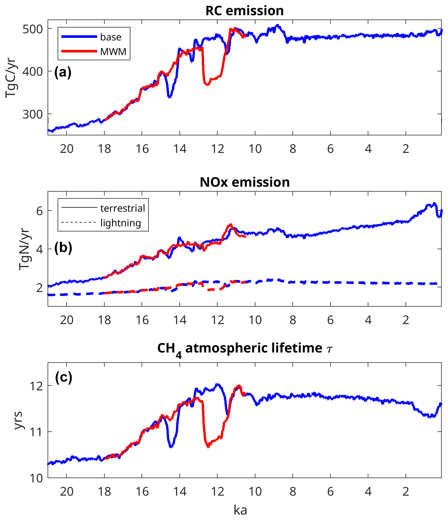
Figure 4 Atmospheric sink of CH₄: emissions of (a) reactive carbon (RC), (b) NO_x from soils and lightning, and (c) the resulting atmospheric lifetime (τ) of CH₄. τ increases with increasing RC and decreases with increasing NO_x.

In both experiments, the simulated atmospheric lifetime of CH₄ (Fig. 4c) varies considerably, from 10.4 years at 20 ka to a maximum of 12 years at 12–11 ka, slowly decreasing throughout most of the Holocene, from 11.8 years at 8 ka to 11.6 years at 2 ka, with a departure to 11.3 years at 1 ka, before reaching 11.6 years during the PI period. Prior to about 8 ka, the variations are dominated by pronounced changes in the RC emissions and CH₄ burden. Note that larger RC emissions and a larger CH₄ burden increase the methane lifetime, whereas larger NO_x emissions have the opposite effect. The general tendency towards higher NO_x emissions dampens the RC-driven increase in the methane lifetime. Consequently, the reduction in RC emissions driven by the meltwater events results in a stronger decrease in the methane lifetime, as the total NO_x emissions are much less affected by these events. LNO_x is reduced, but soil NO_x is unaffected and even slightly increasing. Across the latitudes, the mean atmospheric lifetime of CH₄ is longest in the Southern Hemisphere (SH) extratropics, where values range from 19.5 to 22.5 years (Fig. A1b), whereas lifetimes in the NH extratropics are slightly lower, about 1 year shorter than in the SH. The mean atmospheric lifetimes in the tropics, however, are substantially shorter (Fig. A1c), ranging from 7.2 to 8.3 years.

3.3 The Bølling–Allerød and Younger Dryas

The model experiments that we performed do not display the methane concentration signature expected for the onset of the Bølling–Allerød: an abrupt increase in atmospheric methane between 14.6 and 14.5 ka. Instead, we see an abrupt increase in atmospheric methane at 16.2 ka, 1600 years earlier than expected from palaeoclimate reconstructions. The AMOC signature that would be associated with Heinrich event 1 (H1), a near collapse as recorded in Bermuda rise sediments (McManus et al., 2004; Stanford et al., 2011), is also missing in the model experiments. Due to the absence of the H1, the Bølling–Allerød occurs earlier in our model and is initially of smaller magnitude.

Comparing net CH₄ emissions between the late BA at 13.2 ka in the MWM experiment and 20 ka (Fig. 5), increases in emissions are apparent south of the NH ice sheets as well as in Siberia. The most prominent increase in emissions, however, occurs in the NH tropics, with increases in Africa and Asia being especially prominent. Specifically, northern Africa is substantially wetter and greener than either at the LGM or at present, with the substantial CH₄ emissions from the Sahel region being very striking. The increase in precipitation here leads to an expansion of wetlands and vegetation, and while the wetland expansion increases the methane emitting area, the expansion of vegetation enhances soil carbon content, thereby increasing the substrate available for methane generation.

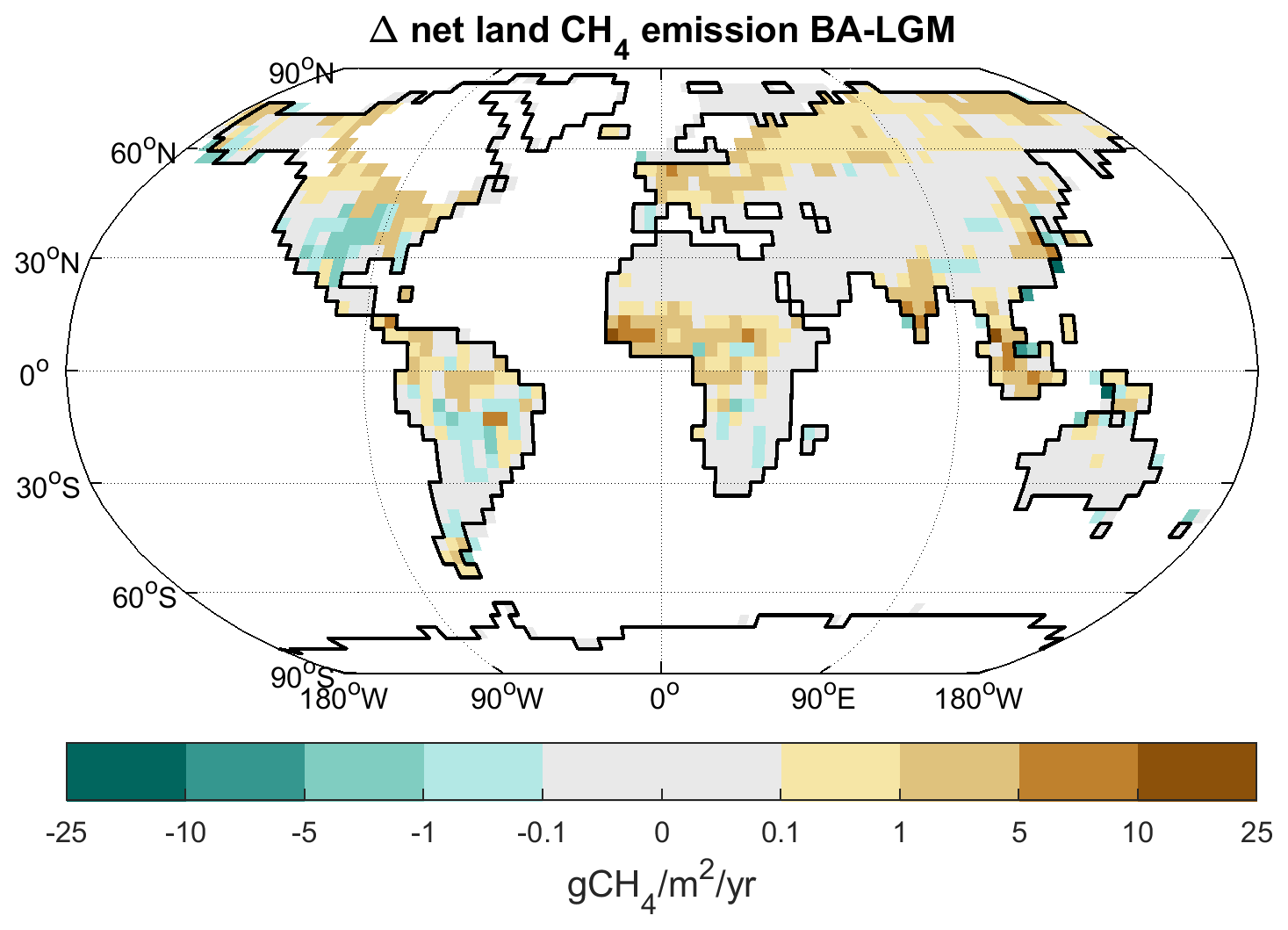
Figure 5 Change in net land CH₄ emissions between the LGM (20 ka) and BA (13.2 ka) in the MWM experiment. Shaded areas indicate LGM land points, and the continental outline is from 13.2 ka.

As the AMOC collapses due to the induced meltwater release at 12.8 ka, the region around the North Atlantic Ocean becomes substantially colder, with temperature decreases exceeding 5 K in large parts of the northern and eastern Atlantic Ocean basin north of the Equator. Precipitation in the NH tropics also decreases significantly, with decreases of more than 1000 mm yr⁻¹ in the tropical Atlantic and precipitation decreases of more than 400 mm yr⁻¹ in the Sahel region as well as over India and Indonesia.

As a result, methane emissions decrease substantially between the BA at 13.2 ka and the YD at 12.5 ka (Fig. 6). Most significant are methane emission reductions throughout the tropics, largely due to reduced precipitation leading to less methane production, but also in Europe, where conditions are substantially colder and dryer during the YD than during the BA.

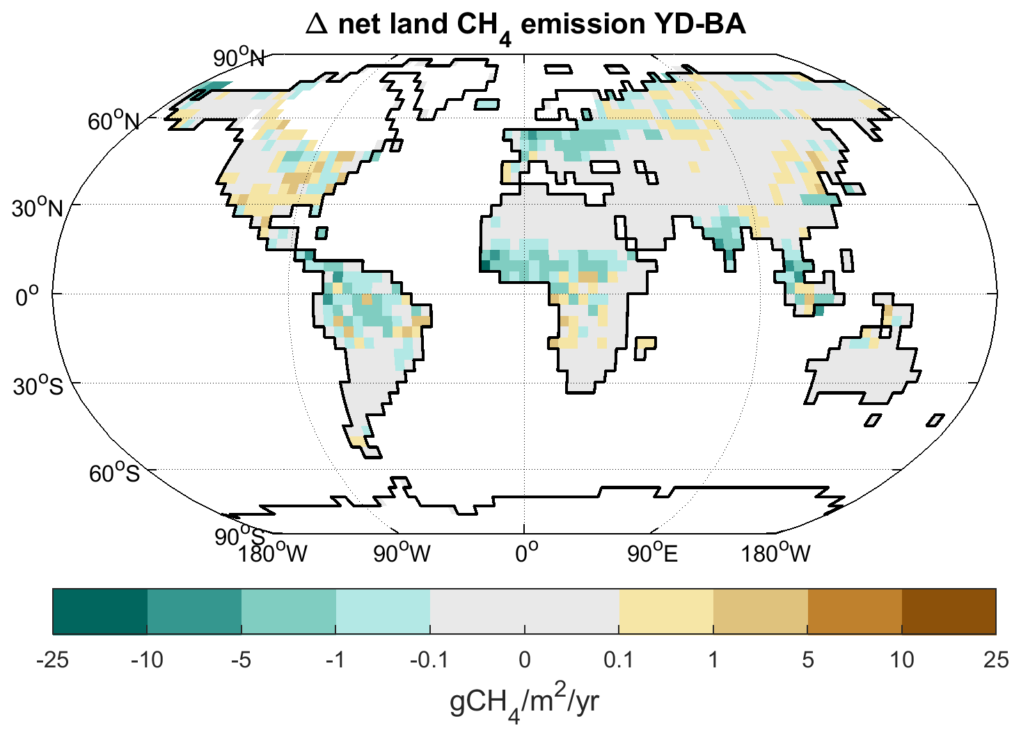
Figure 6 Change in net land CH₄ emissions between the BA (13.2 ka) and YD (12.5 ka) in the MWM experiment. Shaded areas indicate BA land points, and the continental outline is from 12.5 ka.

3.4 The role of exposed shelf areas

Due to the lower sea level in glacial climate, significant areas of the present-day continental shelf were exposed. In our model, 14.2×10⁶ km² of non-glaciated continental shelf that lies below sea level at present was exposed at 20 ka. Slightly more than half this area (7.8×10⁶ km²) was located in tropical latitudes, predominantly in South-East Asia and Australia. In the NH extratropics, some 5×10⁶ km² was exposed, largely in the Laptev Sea and Bering Strait. These areas changed relatively little until 15 ka, but they started decreasing rapidly afterwards. By 7.8 ka, most of these areas were flooded, and the rising sea level covered the remainder at 4.3 ka. Our model shows the exposed shelf areas to be a significant source of methane due to significant vegetation growth and wetland formation. With emissions of 31 Tg CH₄ yr⁻¹, the global shelf areas emitted a significant fraction of the net methane flux at 20 ka (Fig. 7a). Due to global warming, the shelf emissions increased further to 40 Tg CH₄ yr⁻¹ at 15 ka, but they subsequently declined as sea level rise started to submerge these areas. The bulk of this flux – 20 Tg CH₄ yr⁻¹ at 20 ka – is emitted from the extensive shelf areas in South-East Asia (Sunda Shelf) and north-western Australia (Sahul Shelf), combined in Fig. 7b as South-East Asia. Here, emissions increased slightly between 20 and 14 ka, subsequently dropping to near zero by 10 ka. While the AMOC collapse in the MWM experiment does affect the region, decreasing emissions slightly, the effect is less pronounced here than in other regions. In non-tropical regions, the largest exposed shelf area in the Laptev Sea and Bering Strait had emissions of some 3.2 Tg CH₄ yr⁻¹ at 20 ka, which rose to 6.9 Tg CH₄ yr⁻¹ at 14 ka, falling subsequently to zero at 8 ka when the remaining shelf area was flooded.

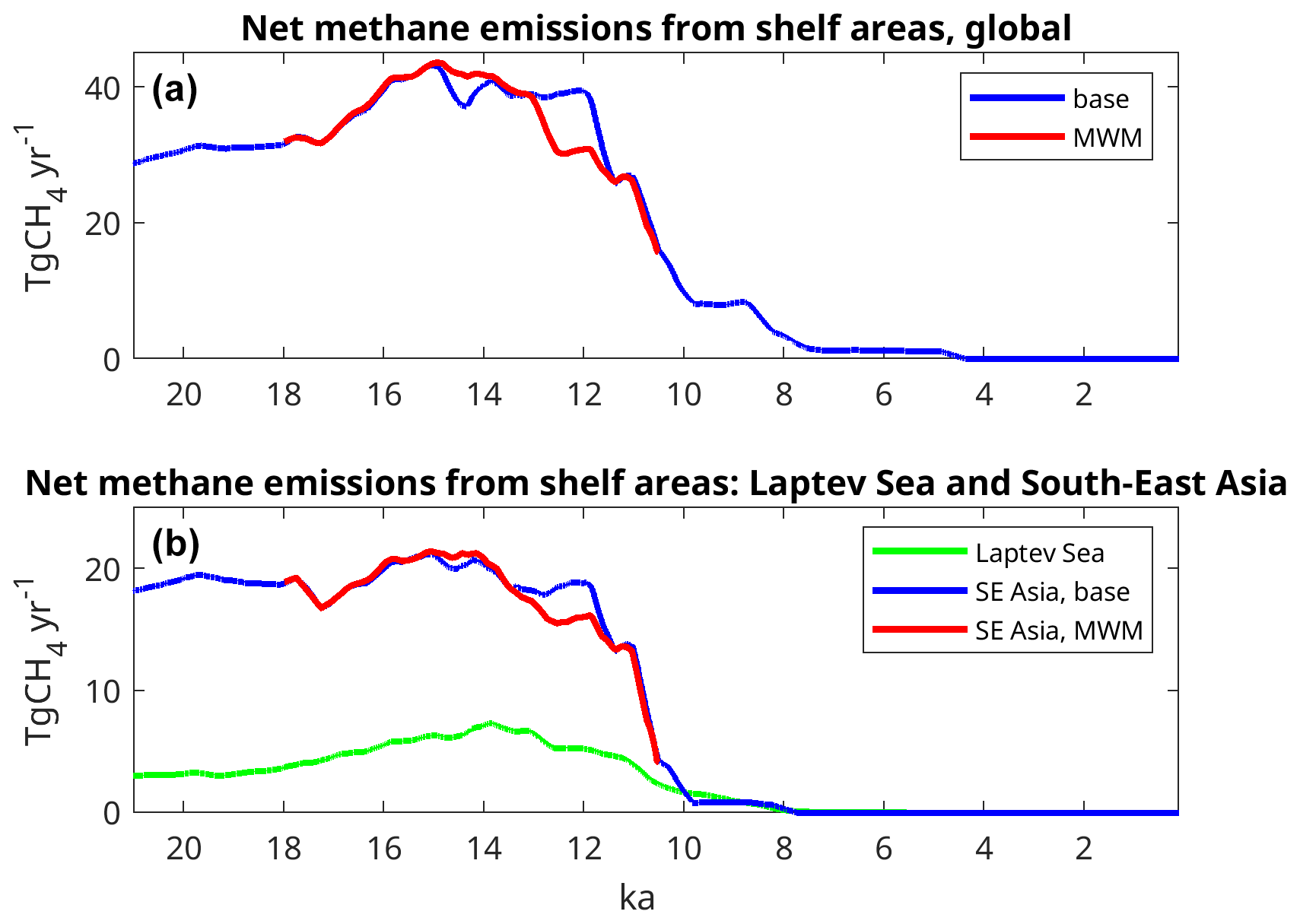
Figure 7 Net methane emissions from shelf areas flooded in a PI climate: (a) global emissions and (b) emissions from the Laptev Sea and South-East Asia.

There were further regions with some shelf methane emissions, but the aforementioned areas cover the most important source regions at 15 ka (Fig. 8). However, the highest net emissions originate from a grid point in the East China Sea, just east of present-day Shanghai. The bathymetric data used to determine wetland area on the shelves indicate a very flat area at this location, which results in a grid-cell mean inundation of nearly 25 % at 15 ka. Whether this high value accurately reflects conditions at the time when the shelf was exposed or whether it is due to subsequent changes in bathymetry caused by the Yangtze River sediment load is an open question that we are not qualified to answer.

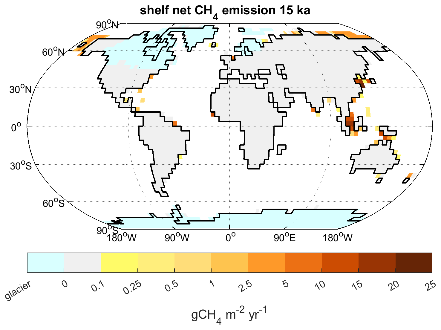
Figure 8 Net shelf CH₄ emissions at 15 ka – the emission maximum. Shaded areas indicate land points at 15 ka, and the continental outline is from the PI state.

3.5 Regional distribution of methane fluxes over time

During the Early Holocene (at 9 ka), the total methane emissions were very similar to the PI state. However, the spatial distribution differed significantly (Fig. 9). Due to the recent deglaciation of North America, with some parts of the Laurentide ice sheet still remaining, CH₄ emissions from North America were strongly reduced, whereas emissions from northern Siberia were enhanced in comparison with the PI period, due to enhanced vegetation growth (and thus soil carbon) from increased solar radiation during the boreal summer season. Furthermore, emissions from South America were reduced. The most striking difference to the PI state, however, was the change in NH tropical Africa. At present, northern Africa is not an important source of methane. Large parts of the continent are rather dry and, thus, do not produce significant amounts of methane. During the Early Holocene, however, the North African monsoon was considerably stronger, leading to significantly enhanced precipitation across the Sahel region, reaching into the southern Sahara (Fig. 10) (Dallmeyer et al., 2020, 2021). As a result, vegetation and wetlands in the Sahel expanded and methane emissions were substantially stronger than during the PI period.

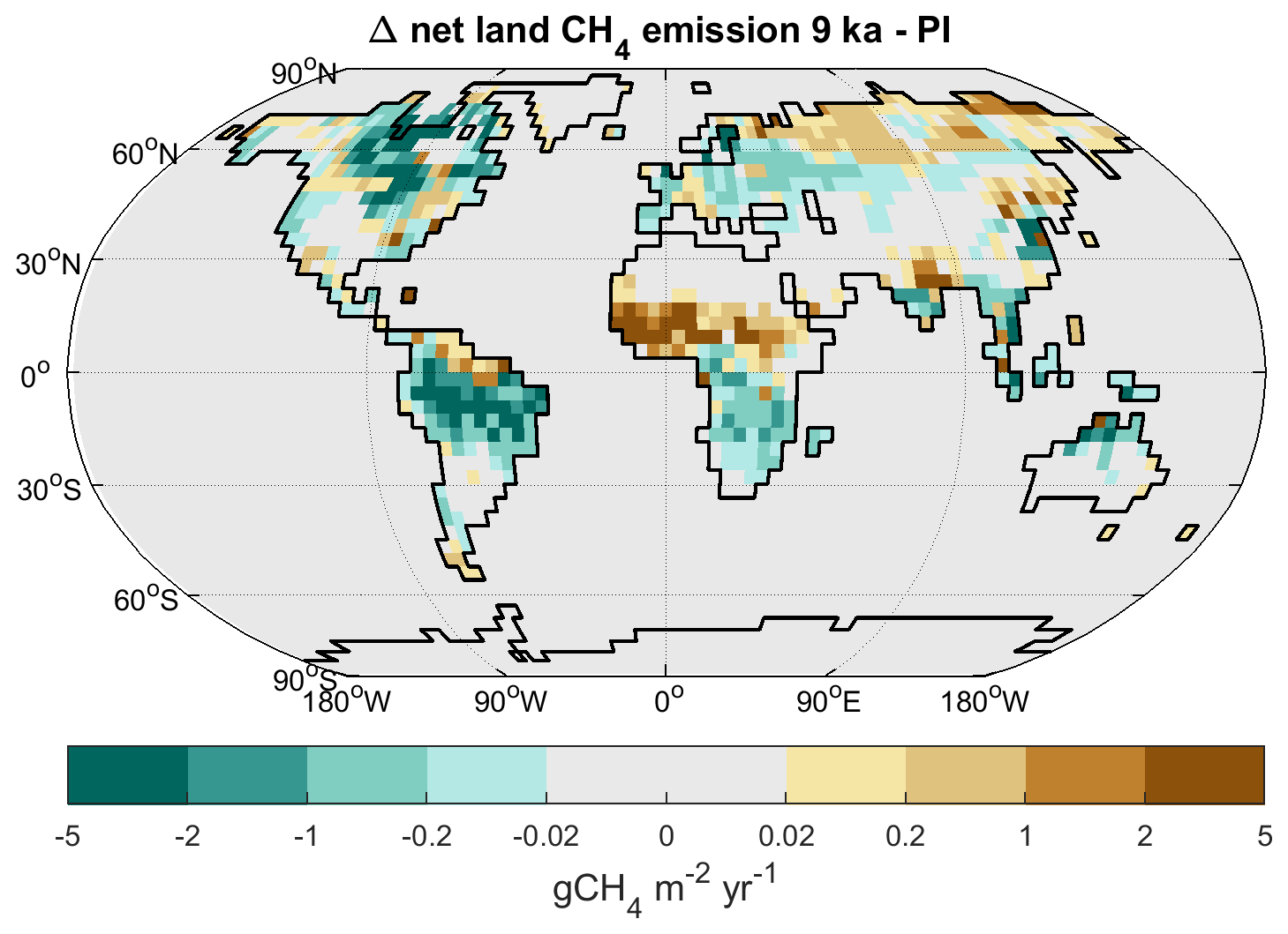
Figure 9 Net CH₄ emission change from 9 ka to the PI period. The continental outline is from 9 ka.

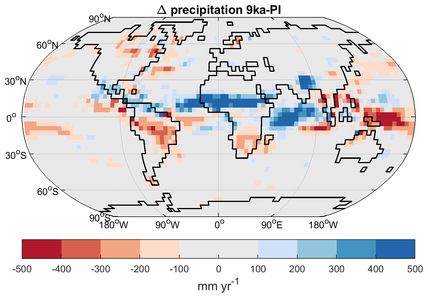
Figure 10 Precipitation change from 9 ka to the PI period. The continental outline is from 9 ka.

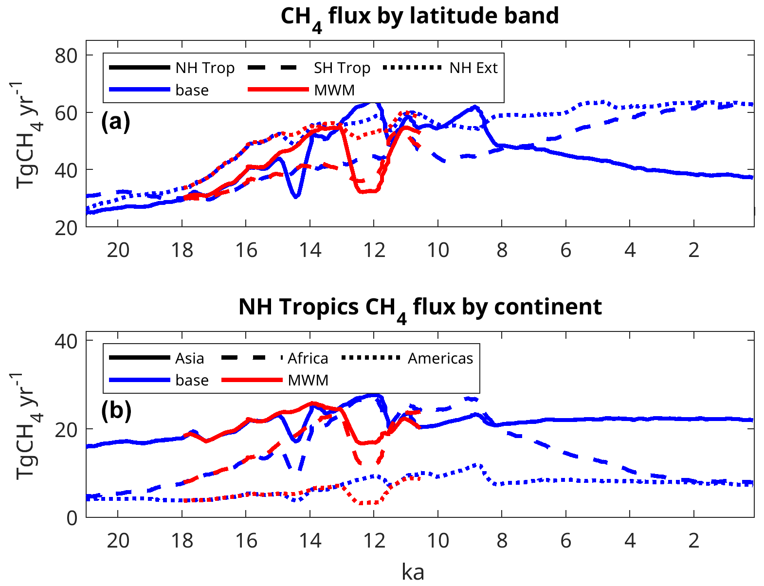
Figure 11 Net CH₄ flux over time by (a) latitude band and (b) continent for the NH tropics (0–30^∘ N).

Looking at the time series of the regional distribution of methane fluxes since the LGM in our experiments, the SH tropics had the largest net emissions at the LGM, with the NH tropics and extratropics each having slightly lower emissions. As emissions increased during the deglaciation, their share from the NH tropics and extratropics increased faster than that from the SH tropics (Fig. 11a). Emissions in the NH extratropics increased markedly between 18 and 11 ka, rising from 33 to 60 Tg CH₄ yr⁻¹ 7000 years later, with little change afterwards. Emissions in the NH tropics, on the other hand, were strongly affected by the AMOC perturbation events, after MWP 1a in the base experiment and at 12.8 ka in the MWM experiment. Here, emissions also started to increase from 30 Tg CH₄ yr⁻¹ at 18 ka, and they continued to rise until they reached 62 Tg CH₄ yr⁻¹ at 9 ka. In the base experiment, this increase was interrupted after MWP 1a; here, CH₄ emissions dropped from 46 to 27 Tg CH₄ yr⁻¹ during the period from 15 to 14.4 ka. In the MWM experiment, on the other hand, emissions in the NH tropics strongly reacted to the imposed Younger Dryas event, with emissions dropping from 55 to 31 Tg CH₄ yr⁻¹ between 12.8 and 12.5 ka. Investigating the changes in the NH tropics by continent (Fig. 11b), it is clear that the bulk of the long-term changes in methane fluxes from this region are from NH tropical Africa, with African CH₄ emissions increasing from 5 Tg CH₄ yr⁻¹ at 20 ka to some 26 Tg CH₄ yr⁻¹ between 13 and 8.5 ka and then subsequently decreasing gradually to 8 Tg CH₄ yr⁻¹ after 2 ka. In comparison to these fluxes from NH Africa, fluxes from NH tropical Asia and America change very little, except for the rapid changes in fluxes from NH tropical Asia connected to AMOC changes after MWP 1a in the base experiment and during the Younger Dryas in the MWM experiment.

Finally, focusing on the Holocene changes after 8 ka, we see a decreasing trend in emissions from the NH tropics (Fig. 11a), whereas emissions from the SH tropics increase. The latter increase is due to a generally increasing trend in precipitation over South America (Fig. 10), leading to increasing emissions from the Amazon region, while the former is due to a decreasing trend in precipitation over NH tropical regions, mainly in Africa, but also over northern India. These precipitation trends are ultimately caused by orbital changes, with the change in precession leading to a decrease in radiation reaching NH tropical areas and an increase in radiation reaching SH tropical areas, causing changes in land–sea temperature contrasts and, thus, changes in monsoon circulation and related precipitation (Dallmeyer et al., 2021). Therefore, we see a very similar trend to Singarayer et al. (2011), who reported decreasing emissions from the NH tropics and increasing emissions from the SH over the last 8 ka. Singarayer et al. (2011) were thus able to explain the Holocene trend in reconstructed CH₄, a decrease from the Early to Middle Holocene followed by an increase from the Middle to Late Holocene. In our model, however, these trends more or less cancel each other out, leading to very small changes in overall methane emissions, despite the substantial changes in regional fluxes.

4 Discussion

The evolution of climate in our transient deglaciation experiment generally seems to be similar to climate reconstructions, with the reconstruction by Shakun et al. (2012) showing smaller changes in global mean temperature and the reconstruction by Osman et al. (2021) showing larger changes. However, regional details may not necessarily agree with reconstructions. Examples here are the freshwater flux from MWP 1a leading to a collapse of the AMOC in the base experiment or the missing H1 Heinrich event leading to an earlier warming related to the BA onset in the base and MWM experiments. One could argue that a model configuration with prescribed ice sheets and meltwater fluxes, as used here, is not capable of simulating a full Heinrich event, as a true Heinrich event is a coupled mode of ice-sheet and ocean dynamics (Ziemen et al., 2019) that requires an interactive ice-sheet model to be captured completely. Nonetheless, our model experiment contains two events that show most of the climatic characteristics of a Heinrich event: the AMOC collapse after MWP 1a in the base experiment and the induced transition into the Younger Dryas in the MWM experiment. The latter event also shows the methane response one would expect from a Heinrich event (Fig. 6): a general decrease in circum-Atlantic methane emissions, possibly extending to further tropical methane emission areas. However, this picture is strongly dependent on the background state: as emissions from Europe are smaller under full glacial conditions than under BA conditions, a Heinrich event under full glacial conditions would lead to a much smaller decrease in emissions than during the Younger Dryas.

Balancing the methane budget over the course of the deglaciation has proven to be very challenging. Flux estimates for some of the methane source fluxes vary widely in the literature and may be quite different from those that we obtain. Bock et al. (2017), for example, estimate (from CH₄ stable isotopes) that the combined flux from biomass burning and geological sources is some 90 Tg CH₄ yr⁻¹ in interglacials and some 70 Tg CH₄ yr⁻¹ in glacials. Along similar lines, Saunois et al. (2020), based on Etiope and Schwietzke (2019), estimate some 45 Tg CH₄ yr⁻¹ for PD geological emissions. Taking the top-down estimate of total natural methane fluxes for the present day from Saunois et al. (2020) of 232 Tg CH₄ yr⁻¹, the Bock et al. (2017) estimate, taken at face value, would imply that about 39 % of the PD natural CH₄ emissions would be from wildfires and geological sources, indicating that a substantial reduction in all other natural sources of methane would be required in order to balance the global CH₄ budget. Our model shows some 165 and 90 Tg CH₄ yr⁻¹ for total net emissions during the PI period and at the LGM, respectively, and the Bock et al. (2017) estimate would thus imply that 54 % of PI emissions and about 78 % of the LGM net methane emissions are from biomass burning and geological sources. Furthermore, the estimates from Saunois et al. (2020) would imply that roughly half of the total LGM methane emissions are of geological origin, as we are not aware of any mechanisms that would lead to lower geological fluxes at the LGM in comparison with the present. The only way to reconcile these flux estimates with reconstructed atmospheric CH₄ concentrations would be to assume that either the atmospheric lifetime of CH₄ was substantially lower at the LGM than at present, which goes against the present understanding of methane chemistry (Murray et al., 2014), or to assume that the other natural sources of methane, especially wetlands which are generally acknowledged to be the largest natural source of CH₄ (Saunois et al., 2020), would be drastically reduced in comparison with our experiments and other estimates. Therefore, we assume that these flux estimates are an overestimate.

Our present publication generally confirms the results from time-slice experiments that we obtained earlier (Kleinen et al., 2020); however, this work importantly integrates a methane sink component into the modelling system and enables the investigation of highly transient changes in methane, such as during the BA–YD transition. Thus, we corroborate that the large-scale change in atmospheric methane from the LGM to the Holocene is mainly due to changes in wetland emissions, with the tropical areas being the main emitting region and the NH extratropics playing a secondary role. This change in wetland emissions can be attributed to increases in soil carbon storage, increases in atmospheric CO₂ and further climate changes, with warming playing the most prominent role (Kleinen et al., 2020). While there are a number of uncertain parameters in the wetland methane emission model, changes in these tend to have very similar effects in both the LGM and PI climate states, proportionally adjusting the emission strengths so that their LGM-to-PI ratio remains little affected. The latter is instead determined by the changes in soil C, atmospheric CO₂ and climate. Therefore, factors like CO₂ fertilisation (the increase in vegetation productivity with increasing atmospheric CO₂) would need to be adjusted in order to affect the LGM-to-PI ratio of CH₄ emissions. As the difference in terrestrial carbon storage between the LGM and the PI period is on the high side (Jeltsch-Thömmes et al., 2019, for example, estimate 450–1250 Pg C for the LGM to PI period change in terrestrial C, including substantial C stores like peatlands that we do not consider in our model), a decrease in CO₂ sensitivity might improve overall results.

We calibrated the contributions of the different methane sources to the total flux to be conformal to the present-day source distribution (Saunois et al., 2016, 2020), and the relative contributions of the single sources to the total emissions change very little over the course of the deglaciation. In terms of total emissions, Valdes et al. (2005) assume LGM emissions of 152.4 Tg CH₄ yr⁻¹ and PI emissions of 198.9 Tg CH₄ yr⁻¹, while Hopcroft et al. (2017) obtain 129.7 Tg CH₄ yr⁻¹ at the LGM and 197.2 Tg CH₄ yr⁻¹ during the PI period. Both of these estimates are higher than our results (net emissions of 90 Tg CH₄ yr⁻¹ at 20 ka and 165 Tg CH₄ yr⁻¹ during the PI period), requiring a shorter atmospheric lifetime of CH₄ than we obtain.

Both Valdes et al. (2005) and Hopcroft et al. (2017) assume oceanic CH₄ emissions, with LGM emissions of the order of 11 Tg CH₄ yr⁻¹ and PI emissions of the order of 14 Tg CH₄ yr⁻¹. We only consider oceanic emissions from geological sources (Etiope, 2015; Saunois et al., 2016, 2020), neglecting biogenic oceanic sources that are assumed to be small. For the geological emissions, the total amount is highly debated at present, with direct measurements showing substantially higher estimates (Etiope, 2015; Mazzini et al., 2021) than ice-core-based reconstructions of emissions during the YD (Petrenko et al., 2017) or PI period (Hmiel et al., 2020). We chose geological emissions of 5 Tg CH₄ yr⁻¹, which is at the upper limit but still compatible with ice-core measurements. Assuming geological emissions of 45 Tg CH₄ yr⁻¹, more in line with Saunois et al. (2020), would make it extremely difficult to match the LGM methane budget, as the geological sources would then make up roughly half of the total emissions, implying an even larger reduction in all other methane fluxes for the LGM in comparison with the PI period than already required.

The modelled wetland emission fluxes are dependent on the inundated area extent as well as on soil carbon content within those inundated areas. Our model overestimates inundation in tropical areas (Kleinen et al., 2020) in comparison with some remote-sensing estimates (Prigent et al., 2012). The latter estimates, however, are based on a combination of optical and radar sensor data and are likely susceptible to the underestimation of inundation in areas with a dense forest canopy, such as tropical rainforests (Melton et al., 2013). Unfortunately, due to a lack of other reference data, reconciling the model and remote-sensing estimates is not possible yet. If we assume that the overestimate of tropical wetland areas is significant, it would decrease tropical emissions, adding more weight to the extratropical areas. However, the modelled wetland methane emission fluxes for the PI and PD climate states (Kleinen et al., 2020, 2021) fall well within the range of wetland fluxes shown in the latest Global Carbon Project Global Methane Budget (Saunois et al., 2020), and the latitudinal distribution of wetland methane emissions is similar to assessments in atmospheric inversion studies (Bousquet et al., 2011), where tropical areas are the source of 62 %–77 % of global wetland emissions. Thus, we conclude that our model generally captures the wetland emissions correctly.

Methane emissions from wildfires range from 3.2 Tg CH₄ yr⁻¹ at the LGM to 10.9 Tg CH₄ yr⁻¹ during the PI period in our experiments; thus, they are substantially lower than the Bock et al. (2017) estimate for combined emissions from wildfires and geological sources. However, some evidence for past wildfires during recent millennia also points towards higher fire occurrence than shown by our model (Marlon et al., 2008; Nicewonger et al., 2020). The SPITFIRE fire model that we use (Lasslop et al., 2014) requires two factors for a fire to occur: a sufficient amount of fuel and an ignition source. The former is a function of climate (biomass, precipitation and temperature), whereas the latter is modulated by either lightning intensity or human activities parameterised using the population density. With less carbon on land (Fig. 1c) at the LGM as well as a much less dense human population, igniting presumably considerably fewer fires, missing wildfire sources would be attributed to underestimated lightning-induced emissions in a glacial climate. However, the lightning model that we use for atmospheric chemistry (Price and Rind, 1992, 1993) indicates that the decrease in lightning in colder climates is due to reduced convective activity (see lightning NO_x in Fig. 4b for comparison), thereby rendering higher fire emissions in a glacial climate less likely. Palaeorecords covering the last 1 (Marlon et al., 2008) to 2 millennia (Nicewonger et al., 2020) indicate a higher fire activity than shown by our model, possibly at levels similar to the present day. However, longer-term studies based on charcoal records from the LGM to the PI period (Power et al., 2008) show an overall increase in fire occurrence over all continents as the deglaciation progresses, which is qualitatively very similar to fire occurrence in MPI-ESM in our study.

With respect to methane emissions from herbivorous mammals, this source category is presently dominated by domesticated animals, mainly cows, and both the densities and the species distributions of wild herbivorous mammals in an Earth system untouched by humans, as we assume it to be for the LGM state, is completely unknown. Thus, we tied the emissions of herbivorous mammals to the net primary production, as a proxy for food availability. Previous estimates (Crutzen et al., 1986; Chappellaz et al., 1993) were derived using a different methodology that involved estimating key species populations and extrapolating emissions from these. Hence, Chappellaz et al. (1993) estimate herbivore emissions of 15 Tg CH₄ yr⁻¹ for the preindustrial Holocene and of 20 Tg CH₄ yr⁻¹ for the LGM, arguing that grasslands expanded by 50 % at the LGM, thereby enlarging the available habitat. In our model experiments, however, we find that grasslands do not expand at the LGM in comparison to the PI period. Instead, grasslands are slightly larger in the PI state compared with the LGM. It may be that the discrepancy in areal estimates is due to Chappellaz et al. (1993) assuming grassland in eastern Siberia at the LGM, but our model instead finds that polar deserts expand in the aforementioned region due to extremely dry conditions. Other estimates of herbivore emissions generally refer back to the estimate of Crutzen et al. (1986), which also forms the basis for the Chappellaz et al. (1993) estimate, and thus do not need to be discussed here further. Smith et al. (2016), however, also estimated Late Pleistocene and preindustrial methane production form herbivorous mammals. They report herbivore emissions of 150 Tg CH₄ yr⁻¹ for the Late Pleistocene, which is slightly less than double our estimate of net total emissions at the LGM. Thus, their estimate would require a dramatically shorter lifetime for atmospheric CH₄ than for the PI state, which is considered incompatible with the current understanding of the methane cycle (Murray et al., 2014; Hopcroft et al., 2017).

The soil uptake of methane is calculated from the diffusion of methane into dry soils, where it is subsequently oxidised. The magnitude of this flux is determined by the rate of diffusion into the soil as well as by the oxidation rate of methane in the soil. Here, we do not consider the potential enhancement of high-latitude methane uptake by high-affinity methanotrophs, as suggested by Oh et al. (2020). In our model, the rate of methane uptake is primarily limited by the rate of diffusion of CH₄ and O₂ into the soil, and the oxidation rate is of secondary importance. An increase in the latter at high latitudes would, thus, have a small impact on total uptake. Depending on its formulation and parameterisation, the mechanism by Oh et al. (2020) might have a greater impact in other models. We also prescribed atmospheric methane concentrations from ice-core data (Köhler et al., 2017) when determining the uptake flux. Obviously there is a small discrepancy in comparison with the flux that we would have obtained if we had used the modelled methane concentration. However, the impact of this discrepancy on the atmospheric methane concentration is small, as modelled and ice-core CH₄ values are very similar to each other for most of the experiment. One exception to this is the mid-Holocene period, when the modelled CH₄ is substantially higher than the reconstruction. Thus, the methane uptake during this period would be higher than that shown here, although not high enough to significantly reduce the CH₄ concentration.

The atmospheric sink of methane in our model is simulated using the total reactivity fields obtained from the EMAC model (Joeckel et al., 2010) modulated according to climate changes as shown in Eq. (2): atmospheric CH₄ removal increases (equivalently decreasing the associated lifetime) with increasing NO_x emission from soils and lightning and reductions in RC emissions. While methane sinks obtained in the EMAC model allow for their recombination into total sink fields (e.g. for isotope-enabled studies), we have used the aggregated sink formulation in the current MPI-ESM experiments which does not allow for the determination of changes in the contributions from the different components over the course of the deglaciation. The reason for this more pragmatic implementation, in addition to optimisation of model simulation resources, is that we attribute most of the variation in the CH₄ sink to changes in tropospheric OH abundance, driven in turn by changes in the emissions of NO_x and RC. Changes to the atmospheric Cl-initiated sink of methane may be important for estimating changes in methane isotope ratios since the PI period (Levine et al., 2011); however, under PI conditions in EMAC, it accounts for less than 0.1 % of the total methane sink, making it substantially less important for the evolution of PI CH₄.

Finally, the mid-Holocene decrease in atmospheric methane is the one aspect of the development of atmospheric methane in the time from the LGM to the PI period that we were unable to reproduce in a satisfactory way. Singarayer et al. (2011) were able to attribute these changes to the orbital forcing. They found that, due to precession-induced insolation changes, wetland emissions from the SH tropics increase after 5 ka, whereas emissions from the NH tropics decrease, with the NH decrease being smaller than the SH increase after 5 ka. We see a very similar behaviour in our model: wetland emissions from the NH tropics, especially from Africa, decrease after 8 ka, whereas emissions from the SH tropics, predominantly the Amazon region, increase (Fig. 11). However, the net result in our case is that the NH decrease is exactly compensated for by the SH increase, leading to no change in total emissions. Thus, our model produces constant emissions from 8 ka to the PI period, leading to a constant atmospheric concentration with neither a decrease before 5 ka nor an increase after 5 ka being apparent. We suspect that this behaviour may be due either to NH extratropical emissions or to the monsoon changes in northern Africa. The total NH extratropical emissions are rather stable over the course of the Holocene (Fig. 11), despite large regional changes (Fig. 9), as changes in one region are compensated for by changes in other regions. On the other hand, the expansion of the African monsoon system in our model is relatively limited in comparison to reconstructions. The latter show an expansion of the monsoon into the Sahara, whereas we only get an increase in the Sahel. The larger extent in the reconstructions would imply a different temporal behaviour with a narrower emission peak. With this change in African emissions, the emission decrease from the NH tropics would be less than the emission increase from the SH tropics, thus leading to the methane trajectory observed in ice cores.

5 Conclusions

Our model experiments demonstrate – for the first time – how the complete methane cycle changes over the course of the deglaciation. We found that the atmospheric lifetime of CH₄ has increased slightly, from 10.4 years at 18 ka to a maximum of 12 years at 12 ka, implying that the observed doubling of the atmospheric CH₄ concentration during this interval has to be explained primarily by changes in CH₄ emissions. The model is capable of simulating such changes in CH₄ sources, with wetland emissions increasing from 80 to 150 Tg CH₄ yr⁻¹ primarily driven by increases in vegetation productivity. We reproduce all major features of the deglacial ice-core methane record, with the exception of the observed mid-Holocene minimum in methane, as a decrease in simulated NH methane sources is perfectly balanced by an increase in SH sources, leading to almost no change in the CH₄ concentration. For much of the deglaciation, our atmospheric transport model reproduces both the Antarctic and Greenland methane records, thus also capturing the interhemispheric gradient.

We are also able to simulate significant emissions of CH₄ from shelf areas that were flooded in the course of the deglaciation. Simulated changes in the total terrestrial carbon storage with respect to an approximate 720 Pg C increase from the LGM to the PI period are at the upper end of modelling estimates.

Some of the abrupt deglacial methane changes, however, cannot be reproduced spontaneously and rather require dedicated model set-ups: as shown in our base experiment (and by Kapsch et al., 2022), an application of meltwater forcing from ice-sheet reconstructions will not lead to climate changes as reconstructed from proxy data. The meltwater input from MWP 1a leads to a collapse of the North Atlantic AMOC circulation and a strong cooling event in circum-Atlantic areas at the time when the Bølling–Allerød warming would rather be expected. With appropriate control of the ice-sheet meltwater, however, we were able to reproduce the entire deglaciation sequence in the MWM experiment. Thus, storing the meltwater from the Laurentide ice sheet and releasing the accumulated meltwater at 12.8 ka leads to a sequence of Bølling–Allerød warming, Younger Dryas cooling and Preboreal warming that is, in terms of atmospheric methane, very close to ice-core records from Antarctica and Greenland.

Appendix A: Additional figures

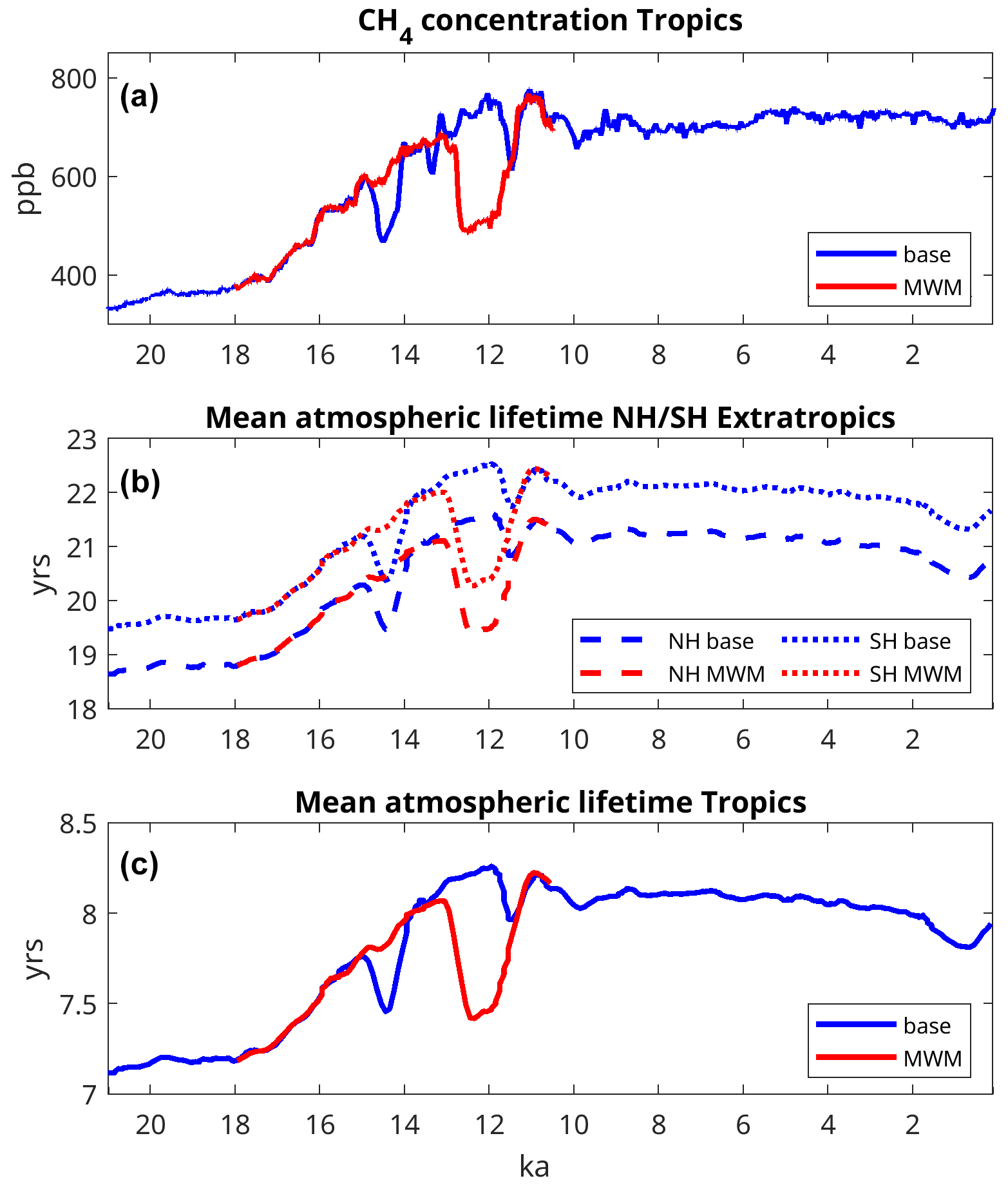
Figure A1 Panel (a) presents the tropical methane concentration. Panels (b) and (c) show the mean atmospheric lifetime of methane at extratropical latitudes and in the tropics, respectively.