Sea ice changes in the southwest Pacific sector of the Southern Ocean during the last 140 000 years

Sea ice expansion in the Southern Ocean is believed to have contributed to glacial–interglacial atmospheric CO₂ variability by inhibiting air–sea gas exchange and influencing the ocean's meridional overturning circulation. However, limited data on past sea ice coverage over the last 140 ka (a complete glacial cycle) have hindered our ability to link sea ice expansion to oceanic processes that affect atmospheric CO₂ concentration. Assessments of past sea ice coverage using diatom assemblages have primarily focused on the Last Glacial Maximum (∼21 ka) to Holocene, with few quantitative reconstructions extending to the onset of glacial Termination II (∼135 ka). Here we provide new estimates of winter sea ice concentrations (WSIC) and summer sea surface temperatures (SSST) for a full glacial–interglacial cycle from the southwestern Pacific sector of the Southern Ocean using the modern analog technique (MAT) on fossil diatom assemblages from deep-sea core TAN1302-96. We examine how the timing of changes in sea ice coverage relates to ocean circulation changes and previously proposed mechanisms of early glacial CO₂ drawdown. We then place SSST estimates within the context of regional SSST records to better understand how these surface temperature changes may be influencing oceanic CO₂ uptake. We find that winter sea ice was absent over the core site during the early glacial period until MIS 4 (∼65 ka), suggesting that sea ice may not have been a major contributor to early glacial CO₂ drawdown. Sea ice expansion throughout the glacial–interglacial cycle, however, appears to coincide with observed regional reductions in Antarctic Intermediate Water production and subduction, suggesting that sea ice may have influenced intermediate ocean circulation changes. We observe an early glacial (MIS 5d) weakening of meridional SST gradients between 42 and 59^∘ S throughout the region, which may have contributed to early reductions in atmospheric CO₂ concentrations through its impact on air–sea gas exchange.

1 Introduction

Antarctic sea ice has been suggested to have played a key role in glacial–interglacial atmospheric CO₂ variability (e.g., Stephens and Keeling, 2000; Ferrari et al., 2014; Kohfeld and Chase, 2017; Stein et al., 2020). Sea ice has been dynamically linked to several processes that promote deep ocean carbon sequestration, namely by (1) reducing deep ocean outgassing by ice-induced “capping” and surface water stratification (Stephens and Keeling, 2000; Rutgers van der Loeff et al., 2014) and (2) influencing ocean circulation through water mass formation and deep-sea stratification, leading to reduced diapycnal mixing and reduced CO₂ exchange between the surface and deep ocean (Toggweiler, 1999; Bouttes et al., 2010; Ferrari et al., 2014). Numerical modelling studies have shown that sea-ice-induced capping, stratification, and reduced vertical mixing may be able to account for a significant portion of the total CO₂ variability on glacial–interglacial timescales (between 40–80 ppm) (Stephens and Keeling, 2000; Galbraith and de Lavergne, 2018; Marzocchi and Jansen, 2019; Stein et al., 2020). However, debate continues surrounding the timing and magnitude of sea ice impacts on glacial-scale carbon sequestration (e.g., Morales Maquede and Rahmstorf, 2002; Archer et al., 2003; Sun and Matsumoto, 2010; Kohfeld and Chase, 2017).

Past Antarctic sea ice coverage has been estimated primarily through diatom-based reconstructions, with most work focusing on the Last Glacial Maximum (LGM), specifically the EPILOG time slice as outlined in Mix et al. (2001), corresponding to 23 to 19 thousand years before present (ka, calibrated backwards from 1950). During the LGM, these reconstructions suggest that winter sea ice expanded by 7–10^∘ latitude (depending on the sector of the Southern Ocean), which corresponds to substantial expansion of total winter sea ice coverage compared to modern observations (Gersonde et al., 2005; Benz et al., 2016; Lhardy et al., 2021). Currently, only a handful of studies provide quantitative sea ice coverage estimates back to the penultimate glaciation, Marine Isotope Stage (MIS) 6 (∼194 to 135 ka) (Gersonde and Zielinksi, 2000; Crosta et al., 2004; Schneider-Mor et al., 2012; Esper and Gersonde 2014a; Ghadi et al., 2020). These studies primarily cover the Atlantic sector, with only one published sea ice record from each of the Indian (SK200-33 from Ghadi et al., 2020), eastern Pacific (PS58/271-1 from Esper and Gersonde, 2014a), and southwestern Pacific sectors (SO136-111 from Crosta et al., 2004). These glacial–interglacial sea ice records show heterogeneity between sectors in both timing and coverage. While the Antarctic Zone (AZ) in the Atlantic sector experienced early sea ice advance corresponding to MIS 5d cooling (i.e., 115 to 105 ka) (Gersonde and Zielinksi, 2000; Bianchi and Gersonde, 2002; Esper and Gersonde, 2014a), the Indian and Pacific sector cores in the AZ show only minor sea ice advances during this time (Crosta et al., 2004; Ghadi et al., 2020). The lack of spatial and temporal resolution has resulted in significant uncertainty in our ability to evaluate the timing and magnitude of sea ice change during a full glacial cycle across the Southern Ocean, and to link sea ice to glacial–interglacial CO₂ variability.

This paper provides new winter sea ice concentration (WSIC) and summer sea surface temperature (SSST) estimates for the southwestern Pacific sector of the Southern Ocean over the last 140 ka. WSIC, which is a grid-scale observation of the mean state fraction of ocean area that is covered by sea ice over the sample period, and SSST estimates are produced by applying the modern analog technique (MAT) to fossil diatom assemblages from sediment core TAN1302-96 (59.09^∘ S, 157.05^∘ E, water depth 3099 m). We place this record within the context of sea ice and SSST changes from the region using previously published records from SO136-111 (56.66^∘ S, 160.23^∘ E, water depth 3912 m), which has recalculated WSIC and SSST estimates presented in this study, and nearby marine core E27-23 (59.61^∘ S, 155.23^∘ E, water depth 3182 m) (Ferry et al., 2015). Using these records, we compare the timing of sea ice expansion to early glacial–interglacial CO₂ variability to test the hypothesis that the initial CO₂ drawdown (∼115 to 100 ka) resulted from reduced air–sea gas exchange in response to sea ice capping and surface water stratification (Kohfeld and Chase, 2017). We then consider alternative oceanic drivers of early atmospheric CO₂ variability and place our SSST estimates within the context of other studies to examine how regional cooling and a weakening in meridional SST gradients might affect air–sea disequilibrium and early CO₂ drawdown (Khatiwala et al., 2019). Finally, we compare our WSIC estimates with regional reconstructions of Antarctic Intermediate Water (AAIW) production and subduction variability using previously published carbon isotope analyses on benthic foraminifera from intermediate to deep-water depths in the southwest Pacific sector of the Southern Ocean, to test the hypothesis that sea ice expansion is dynamically linked to AAIW production and variability (Ronge et al., 2015).

2 Methods

2.1 Study site and age determination

We reconstruct diatom-based WSIC and SSST using marine sediment core TAN1302-96 (59.09^∘ S, 157.05^∘ E, water depth 3099 m) (Fig. 1). The 364 cm core was collected in March 2013 using a gravity corer during the return of the RV Tangaroa from the Mertz Polynya in eastern Antarctica (Williams, 2013). The core is situated in the western Pacific sector of the Southern Ocean, on the southwestern side of the Macquarie Ridge, approximately 3–4^∘ south of the average position of the Polar Front (PF) at 157^∘ E (Sokolov and Rintoul, 2009).

Figure 1 Map of the southwestern Pacific sector of the Southern Ocean including the study site, TAN1302-96 (blue circle), and additional published cores providing sea ice extent data, SO136-111 and E27-23 (green circles); SST reconstructions (red circles); and δ¹³C of benthic foraminifera (yellow circles). Note that some cores may not appear present in the figure because of their proximity to other cores. Data for all cores are provided in Table 2. Dashed lines show the average location of the subtropical and polar fronts (Smith et al., 2013; Bostock et al., 2015), and red and blue lines show mean positions of modern summer sea ice (SSI) and winter sea ice (WSI) extents, respectively (Reynolds et al., 2002, 2007).

The age model for TAN1302-96 (Figs. 2 and 3) was based on a combination of radiocarbon dating of mixed foraminiferal assemblages and stable oxygen isotope stratigraphy on Neogloboquadrina pachyderma (180–250 µm). Seven accelerator mass spectrometry (AMS) ¹⁴C samples were collected (Table A1 in Appendix A) and consisted of mixed assemblages of planktonic foraminifera (N. pachyderma and Globigerina bulloides, >250 µm). Three of the seven radiocarbon samples (NZA 57105, 57109, and 61429) were previously published in Prebble et al. (2017), and four additional samples (OZX 517-520) were added to improve the dating reliability (Table A1 in Appendix A). OZX 519 and OZX 520 produced dates that were not distinguishable from the background (>57.5 ka) and were subsequently excluded from the age model. The TAN1302-96 oxygen isotopes were run at the National Institute of Water and Atmospheric Research (NIWA) using the Kiel IV individual acid-on-sample device and analysed using Finnigan MAT 252 mass spectrometer. The precision is ±0.07 % for δ¹⁸O and ±0.05 % for δ¹³C.

Figure 2 Age model of TAN1302-96. Red circles indicate the depth of AMS ¹⁴C samples, and yellow circles indicate tie points between the TAN1302-96 oxygen isotope stratigraphy and the LR04 benthic stack (Lisiecki and Raymo, 2005). Two radiocarbon dates, OZX 519 and 520 (at 130 and 170 cm, respectively), were not included in the age model as they produced dates that were NDFB (not distinguishable from the background).

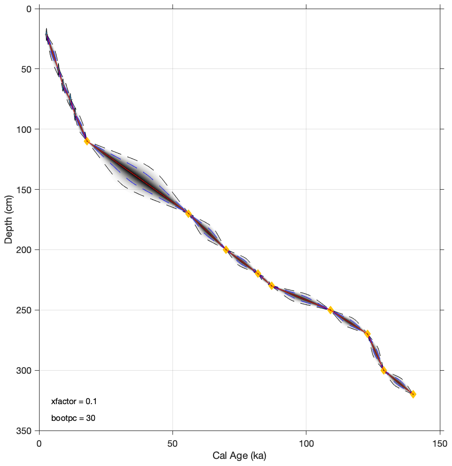
Figure 3 Age model of TAN1302-96. Tie points are depicted as yellow dots, and grey shading represents associated uncertainty between tie points. The age model used a marine reservoir calibration of 1000±100 years.

The age model was constructed using the “Undatable” MATLAB software (Lougheed and Obrochta, 2018) by bootstrapping at 10 % and using an xfactor of 0.1 (Lougheed and Obrochta, 2019), which scales Gaussian distributions of sediment accumulation uncertainty (Table A2 in Appendix A). Below 100 cm, nine tie points were selected at positions of maximum change in δ¹⁸O and were correlated to the LR04 benthic stack (Lisiecki and Raymo, 2005) (Fig. 2; Table A2 in Appendix A). Uncertainty associated with stratigraphic correlation to the LR04 stack has been estimated to be ±4 ka (Lisiecki and Raymo, 2005). We used a conservative marine reservoir age (MRA) for radiocarbon calibration of 1000±100 years, in line with regional estimates in Paterne et al. (2019) and modelled estimates by Butzin et al. (2017, 2020). The age model shows that TAN1302-96 extends to at least 140 ka, capturing a full glacial–interglacial cycle. Linear sedimentation rates in TAN1302-96 were observed to be higher during interglacial periods, averaging ∼3.5 cm ka⁻¹, compared to glacial periods, averaging ∼2.5 cm ka⁻¹. It is worth noting that there can be significant MRA variability over time due to changes in ocean ventilation, sea ice coverage, and wind strength, specifically in the polar high latitudes (Heaton et al., 2020), and as a result, caution should be taken when interpreting the precision of radiocarbon dates. For more information on age model construction and selection, refer to the Supplement.

2.2 Diatom analysis

TAN1302-96 was sampled every 3–4 cm throughout the core except between 130–180 cm, where samples were collected every 10 cm due to limited availability of sample materials (Table A3 in Appendix A). Diatom slide preparation followed two procedures. The first approach approximated the methods outlined in Renberg (1990), while the second followed the protocol outlined in Warnock and Scherer (2015). To ensure there were no biases between preparation techniques, results from each technique were first visually compared followed by a comparison of sample means (see Fig. B1 in Appendix B). No biases in the data were observed between methods.

The first procedure was conducted at Victoria University of Wellington and Simon Fraser University on samples every 10 cm throughout the core. Sediment samples contained high concentrations of diatoms with little carbonaceous or terrigenous materials, so no dissolving aids were used. Instead, approximately 50 mg of sediment was weighed, placed into a 50 mL centrifuge tube, and topped up with 40 mL of deionized water. Samples were then manually shaken to disaggregate sediment, followed by a 10 s mechanical stir using a vortex machine. Samples were then left to settle for 25 s. A total of 0.25 mL of the solution was then pipetted onto a microscope slide from a consistent depth, where it was left to dry overnight. Once the sample had dried, coverslips were permanently mounted to the slide using Permount, a high refractive index mountant. Slides were redone if they contained too many diatoms and identification was not possible, or if they contained too few diatoms (generally <40 specimens per transect). Sediment sample weight was adjusted to achieve the desired dilution.

The second procedure was conducted at Colgate University on samples every 3–4 cm throughout the core. Oven-dried samples were placed into a 20 mL vial with 1–2 mL of 10 % H₂O₂ and left to react for up to several days, followed by a brief (2–3 s) ultrasonic bath to disaggregate samples. The diatom solution was then added into a settling chamber, where microscope coverslips were placed on stages to collect settling diatoms. The chamber was gradually emptied through an attached spigot, and samples were evaporated overnight. Cover slips were permanently mounted onto the slides with Norland Optical Adhesive 61, a mounting medium with a high refractive index.

Diatom identification was conducted at Simon Fraser University using a Leica Leitz DMBRE light microscope using standard microscopy techniques. Following transverses, a minimum of 300 individual diatoms were identified at 1000× magnification from each sample throughout the core. Individuals were counted towards the total only if they represented at least one-half of the specimen so that fragmented diatoms were not counted twice. Identification was conducted to the highest taxonomic level possible, either to the species or species-group level. Taxonomic identification was conducted using numerous identification materials, including (but not limited to) Fenner et al. (1976), Fryxell and Hasle (1976, 1980), Johansen and Fryxell (1985), Hasle and Syversten (1997), Cefarelli et al. (2010), and Wilks and Armand (2017). The relative abundances were calculated by dividing the number of identified specimens of a particular species by the total number of identified diatoms from the sample. Based on previously established taxonomic groups (Crosta et al., 2004), diatoms were grouped into one of three categories based on temperature preference and sea ice tolerance. The following main taxonomic groups were used (Table 1):

1. Sea ice group. This represents diatoms that thrive in or near the sea ice margin in SSTs generally ranging from −1 to 1 ^∘C.

2. Permanently Open Ocean Zone (POOZ). This represents diatoms that thrive in open ocean conditions, with SSTs generally ranging from ∼2 to 10 ^∘C.

3. Sub-Antarctic Zone (SAZ). This represents diatoms that thrive in warmer sub-Antarctic waters, with SSTs generally ranging from 11 to 14 ^∘C.

Table 1 Species comprising each of the diatom taxonomic groups (updated from Crosta et al., 2004).

2.3 Modern analog technique

Past WSIC and SSST (January to March) were estimated for TAN1302-96 and recalculated for SO136-111 by applying the modern analog technique (MAT) to the fossil diatom assemblages, as outlined in Crosta et al. (1998, 2020). Summer (January to March) SST was estimated because it is considered to be a better explanatory variable than spring or annual SST (Esper et al., 2010; Esper and Gersonde, 2014b). The MAT reference database used for this analysis is comprised of 249 modern core top samples (analogs) located primarily in the Atlantic and Indian sectors from ∼40^∘ S to the Antarctic coast. The age of the core tops included in the reference database have been assessed through radiocarbon and/or isotope stratigraphy when possible. Core tops were visually evaluated for selective diatom dissolution, so it is believed that sub-modern assemblages contain well-preserved and unbiased specimens. Modern SSST and WSIC were interpolated from the reference core locations using a $\mathrm{1}{}^{\circ }\times \mathrm{1}{}^{\circ }$ grid from the World Ocean Atlas (Locarnini et al., 2013) through the Ocean Data View (Schlitzer, 2005). The MAT was applied using the “bioindic” package (Guiot and de Vernal, 2011) through the R platform. Fossil diatom assemblages were compared to the modern analogs using 33 species or species groups to identify the five most similar modern analogs using both the LOG and CHORD distance. The dissimilarity threshold, above which the fossil assemblages are considered to be too dissimilar to the modern dataset, is fixed at the first quartile of random distances (Crosta et al., 2020). The reconstructed SSST and WSIC are the distance-weighted mean of the climate values associated with the selected modern analog (Guiot et al., 1993; Ghadi et al., 2020). Both MAT approaches produce an R² value of 0.96 and a root mean square error of prediction (RMSEP) of ∼1 ^∘C for SSST and an R² of 0.93 and a RMSEP of 10 % for WSIC (Ghadi et al., 2020). As outlined in Ferry et al. (2015), we consider <15 % WSIC to represent an absence of winter sea ice, 15 %–40 % WSIC as present but unconsolidated, and >40 % to represent consolidated winter sea ice.

2.4 Additional core data

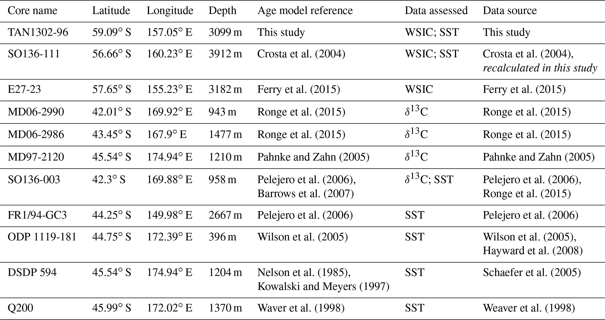
We use additional published marine cores from the southwestern Pacific throughout this analysis (Table 2), for WSIC comparisons (E27-23), %AAIW calculations (MD06-2990/SO136-003, MD06-2986, and MD97-2120), and regional SST gradient comparisons (SO136-003, FR1/94-GC3, ODP 1119-181, DSDP 594, and Q200).

Table 2 Additional data on published marine cores used throughout this analysis.

3 Results

3.1 TAN1302-96 diatom assemblage results

In this core, 51 different species or species groups were identified, of which 33 were used in the transfer function. These 33 species represent >82 % of the total diatom assemblages (mean of 92 %). Permanently Open Ocean Zone (POOZ) diatoms made up the largest proportion of diatoms identified, representing between 72 %–91 % of the assemblage (Fig. 4), with higher values observed during warmer interstadial periods of MIS 1, 3, and 5. Sea ice diatoms made up the second most abundant group, representing between 0.5 %–7.5 % of the assemblage, with higher values observed during cooler stadial periods (MIS 2, 4, and 6). The Sub-Antarctic Zone group had relatively low abundances, with higher values occurring during warmer interstadial periods (MIS 5 and the Holocene) and briefly during MIS 4 at ∼65 ka.

Figure 4 Diatom assemblages results from TAN1302-96 separated into percentage contribution from each taxonomic group (sea ice group, POOZ, and SAZ; see Table 1) over a full glacial–interglacial cycle. Using the modern analog technique (MAT), winter sea ice concentration (WSIC) and summer sea surface temperature (SSST) were estimated and compared against the δ¹⁸O signature of TAN1302-96.

3.2 TAN1302-96 SSST and WSIC estimates

There were no non-analog conditions observed in TAN1302-96 samples, and all estimates were calculated on five analogs. Estimates of SSST and WSIC from both LOG and CHORD MAT outputs produced similar results (Fig. 4). During Termination II, SSST began to rise from ∼1 ^∘C at 140 ka (MIS 6) to ∼4.5 ^∘C at 132 ka (MIS 5e–6 boundary). This warming corresponded with a decrease in WSIC from 48 % to approximately 0 % over the same time periods (Fig. 4). Reconstructed SSSTs were variable throughout MIS 5e, reaching a maximum value of ∼4.5 ^∘C at 118 ka, after which they declined throughout MIS 5. During this period of SSST decline, winter sea ice was largely absent, punctuated by brief periods during which sea ice was present but unconsolidated (WSIC $=\sim \mathrm{15}$ % and 17 % at 105 and 85 ka, respectively). During MIS 4 (71 to 57 ka), SSST cooled to between roughly 1 and 3 ^∘C, and sea ice expanded to 36 %, such that it was present but unconsolidated for intervals of a few thousand years. SSST increased slightly from 1.5 ^∘C at 61 ka (during MIS 4) to ∼2.5 ^∘C at 50 ka (during MIS 3), followed by a general cooling trend into MIS 2. Sea ice appears to have been largely absent during MIS 3 (57 to 29 ka), although sampling resolution is low, but increased rapidly to 48 % cover during MIS 2 where winter sea ice was consolidated over the core site. During MIS 2, SSST cooled to a minimum of <1 ^∘C at 24.5 ka. After 18 ka, the site rapidly transitioned from cool, ice-covered conditions to warmer, ice-free winter conditions during the early deglaciation. This warming was interrupted by a brief cooling around 13.5 ka, following which SSSTs quickly reached their maximum values of ∼5 ^∘C at 11.5 ka and remained relatively high throughout the rest of the Holocene. Winter sea ice was not present during the Holocene.

3.3 SO136-111 SSST and WSIC recalculation

In core SO136-111, the 33 species included in the transfer function represent values >79 % of the total diatom assemblages (mean of 91 %). There were no non-analog conditions observed in SO136-111 samples, and all estimates were calculated on five analogs. Recalculated estimates of SSST and WSIC from both LOG and CHORD MAT outputs produced similar results for SO136-111 (Fig. 5a, d). During Termination II, SSST rose from ∼2 ^∘C at 137 ka (MIS 6) to a maximum value of 6 ^∘C at 125 ka (MIS5e), corresponding to a rapid decline in WSIC from 37 % to ∼0 % during the same period. SSST remained relatively high (between 4 and 5 ^∘C) from 125 ka until 115 ka where they declined to ∼2 ^∘C. SSST remained variable from 110 ka until ∼40 ka, fluctuating between ∼2 and 4 ^∘C. Winter sea ice was largely absent during MIS 5, with a brief period where sea ice was present but unconsolidated (WSIC =17 % at 84 ka). Beginning at ∼76 ka, WSIC began to increase and continued throughout early MIS 4 to a maximum 36 % at 69 ka. WSIC remained present but unconsolidated throughout most of MIS 3 and 2 with brief periods of absence (WSIC ≤15 %) lasting a few thousand years. SSST and WSIC reached their coolest values and highest concentration at 24.5 ka before SSST increased to ∼5 ^∘C and stabilized throughout the Holocene, while WSIC declined to virtually 0 % throughout the same period.

4 Discussion

4.1 Regional SSST and WSIC estimates

The new WSIC and SSST estimates from TAN1302-96 and recalculated WSIC estimates from SO136-111 show a coherent regional pattern (Fig. 5). TAN1302-96 shows slightly higher concentrations during MIS 2 (maximum WSIC =48 % at 24.5 ka) and 4 (maximum WSIC =37 % at 65 ka) compared with SO136-111 (maximum WSIC =35 % at 24.5 ka and 36 % at 68 ka, respectively), which can be explained by a more poleward position of TAN1302-96 relative to SO136-111. The estimates between cores differ during MIS 3, with seemingly lower WSIC in TAN1302-96 than in SO136-111, which might result from the low sampling resolution in TAN1302-96 during this period. Overall, these cores show a highly similar and coherent history of sea ice over the last 140 ka.

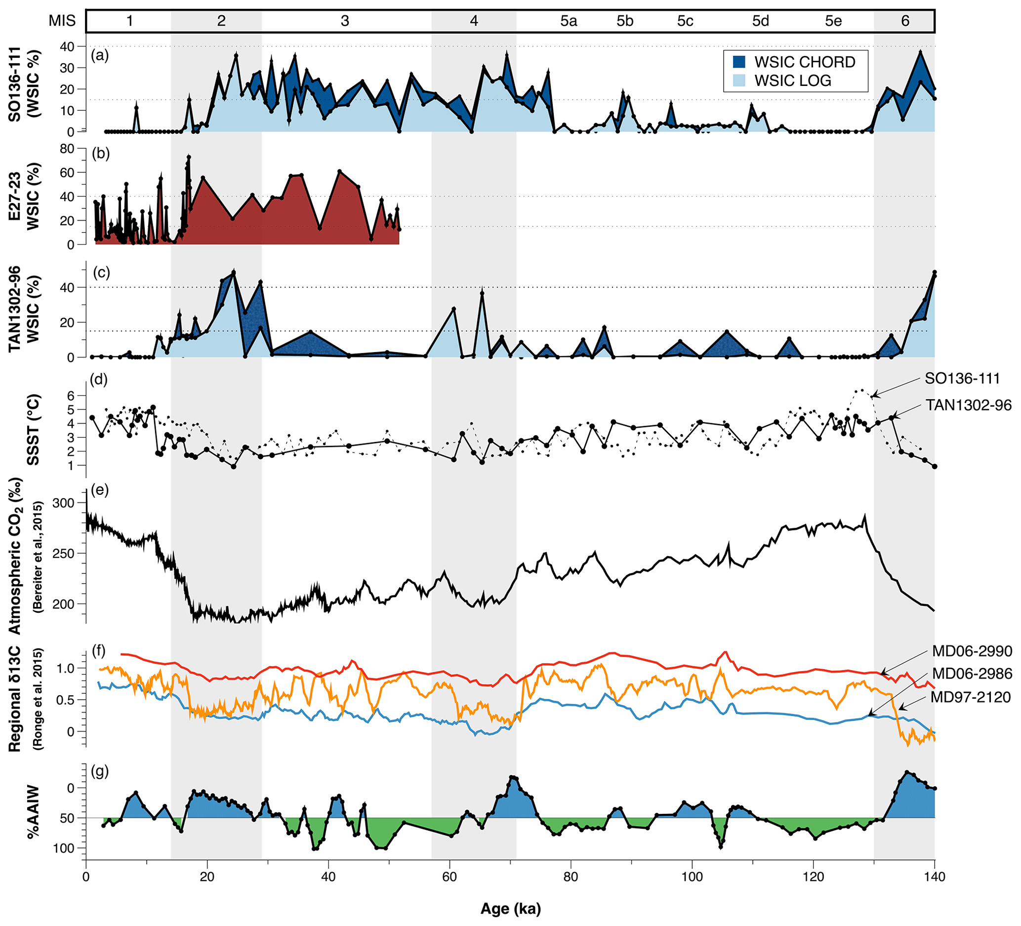
Figure 5 (a) WSIC estimates using MAT from SO136-111 (recalculated in this study; see Appendix D); (b) WSIC estimates using GAM from E27-23 (Ferry et al., 2015); (c) WSIC estimates using MAT from TAN1302-96 (this study); (d) SSST estimates using MAT from TAN1302-96 (solid black line) and recalculated SSST for SO136-111 (black dotted line); (e) Antarctic atmospheric CO₂ concentrations over 140 ka (Bereiter et al., 2015); (f) δ¹³C data from nearby cores MD06-2990/SO136-003, MD97-2120, and MD06-2986 (Ronge et al., 2015); (g) %Antarctic Intermediate Water (%AAIW) as calculated in Ronge et al. (2015), which tracks when core MD97-2120 was bathed primarily by AAIW (green) or Upper Circumpolar Deep Water (UCDW) (blue).

When compared with E27-23 (Fig. 5b), which is located only ∼120 km to the southwest of TAN1302-96 (Fig. 1), the TAN1302-96 core shows lower estimates of WSIC, especially during MIS 3. During early and mid-MIS 2, both cores show similar WSIC estimates, while later in MIS 2 (∼17 ka), E27-23 reports a maximum WSIC of 72 % compared to only 22 % at TAN1302-96. A discrepancy between estimates is also observed during the Holocene, with E27-23 reporting sea ice estimates of up to nearly 50 % during the mid-Holocene (∼6 ka), while TAN1302-96 experienced values well below the RMSEP of 10 %.

Possible explanations for the observed differences in WSIC estimates include (1) differences in statistical applications, (2) lateral sediment redistribution, (3) differences in laboratory protocols, (4) differences in diatom identification/counting methodology, and (5) selective diatom dissolution. Of these explanations, we believe that (1) and (2) are the most likely candidates and are discussed below (for further discussion on 3, 4, and 5, see Appendix C).

The first possible explanation is the use of different statistical applications. Ferry et al. (2015) used a generalized additive model (GAM) to estimate WSIC for both E27-23 and SO136-111, while we have used the MAT for TAN1302-96 and SO136-111. A simple comparison of WSIC estimates between the results in Ferry et al. (2015) and our recalculated WSIC estimates for SO136-111 can provide insights into the magnitude of estimation differences. Generally speaking, the GAM estimation produced higher WSIC estimates than the MAT (e.g., ∼50 % WSIC at 23 ka while the MAT produced ∼37 % for the same time period); however, we believe it is unlikely that statistical approaches alone could explain a larger difference (i.e., 50 %) between E27-23 and TAN1302-96.

The second possible explanation involves lateral sediment redistribution and focusing by the ACC. We estimated sediment focusing for E27-23 using ²³⁰Th data from Bradtmiller et al. (2009) together with dry bulk density estimated using calcium carbonate content (Froelich, 1991). Both sedimentation rates and focusing factors (FF) for the E27-23 are relatively high (maximum ≅35 cm ka⁻¹ and 26, respectively) during the LGM and Holocene, which could influence the reliability of WSIC and SSST estimation (see Fig. C1 in Appendix C). Several peaks in focusing occurring around 16, 12, and 3 ka appear to closely correspond to periods of peak WSIC (∼67 %, ∼54 %, and ∼35 %, respectively), suggesting a possible link. Lateral redistribution could artificially increase or decrease relative abundances of some diatom groups, which could lead to over- or under-estimations of sea ice coverage. Thorium analysis for TAN1302-96 is beyond the scope of this study; however, future work could help address this uncertainty.

Although we are unable to identify the specific cause of the differences, we suggest considering the results from all cores when drawing conclusions of regional sea ice history.

4.2 The role of sea ice on early CO₂ drawdown

Kohfeld and Chase (2017) hypothesized that the initial drawdown of atmospheric CO₂ (∼35 ppm) during the glacial inception of MIS 5d (∼115 to 100 ka) was primarily driven by sea ice capping and a corresponding stratification of surface waters, which reduced the CO₂ outgassing of upwelled carbon-rich waters. This hypothesis is supported by several lines of evidence, including (1) sea salt sodium (ssNA) archived in Antarctic ice cores, suggesting sea ice expansion near the Antarctic continent (Wolff et al., 2010); (2) δ¹⁵N proxy data from the central Pacific sector of the Southern Ocean, suggesting increased stratification south of the modern-day Antarctic Polar Front (Studer et al., 2015); and (3) diatom assemblages in the Permanently Open Ocean Zone (POOZ) of the Atlantic sector, suggesting a slight cooling and northward expansion of sea ice during MIS 5d (Bianchi and Gersonde, 2002). Our data address this hypothesis by providing insights into early sea ice expansion into the polar frontal zone of the western Pacific sector.

Our data show that, in contrast to the Atlantic sector (Bianchi and Gersonde, 2002), there does not appear to be any evidence of sea ice expansion in the southwestern Pacific during MIS 5d at either the TAN1302-96 or SO136-111 core sites (Fig. 5). Unfortunately, the lack of spatially extensive quantitative records extending back to Termination II limits our ability to estimate the timing and magnitude of sea ice changes for regions poleward of 59^∘ S in the southwestern Pacific. We anticipate, however, that an advance in the sea ice edge, consistent with those outlined in Bianchi and Gersonde (2002), likely would have reduced local SST as the sea ice edge advanced closer to the core site. Indeed, the TAN1302-96 SSST record does show a decrease to ∼2 ^∘C (observed at 108 ka), which quickly rebounded to ∼4 ^∘C by ∼102 ka (Fig. 5). However, this SSST drop occurred roughly 7 ka after the initial CO₂ reduction, suggesting that the CO₂ drawdown event and local SSST reduction may not be linked. Thus, while we cannot rule out the possibility of modest sea ice advances or consolidation of pre-existing sea ice (particularly to the south of the core sites), the quantitative WSI and SSST reconstructions suggest that sea ice cover over our core site was limited during glacial inception.

Given that sea ice was not at its maximum extent during the early glacial, it stands to reason that any reductions to air–sea gas exchange in response to the hypothetically expanded sea ice would not have been at its maximum impact either. Previous modelling work has suggested that the maximum impact of sea ice expansion on glacial–interglacial atmospheric CO₂ reductions ranged from 5 to 14 ppm (Kohfeld and Ridgwell, 2009). More recent modelling studies are consistent with this range, suggesting a 10 ppm reduction (Stein et al., 2020), while some studies even suggest a possible increase in atmospheric CO₂ concentrations due to sea ice expansion (Khatiwala et al., 2019). Furthermore, Stein et al. (2020) suggest that the effects of sea ice capping would have taken place after changes in deep ocean stratification had occurred and would have contributed to CO₂ drawdown later during the mid-glacial period. These model results, when combined with our data, suggest that even if modest sea ice advances did take place during the early glacial (i.e., MIS 5d), their impacts on CO₂ variability likely would have been modest, ultimately casting doubt on the hypothesis that early glacial CO₂ reductions of 35 ppm can be linked solely to the capping and stratification effects of sea ice expansion.

4.3 Other potential contributors to early glacial CO₂ variability

The changes observed in WSIC and SSST from TAN1302-96 suggest that sea ice expansion was likely not extensive enough early in the glacial cycle for a sea ice capping effect to be solely responsible for early atmospheric CO₂ drawdown. This leaves open the question of what may have contributed to early drawdown of atmospheric CO₂. In terms of the ocean's role, we highlight three contenders: (1) a potentially non-linear response between sea ice coverage and CO₂ sequestration potential, (2) links between sea ice expansion and early changes in global ocean overturning, and (3) the impact of cooling on air–sea disequilibrium in the Southern Ocean.

The first possible explanation considers that not all sea ice has the same capacity to facilitate or inhibit air–sea gas exchange. We previously suggested that because sea ice was not at its maximum extent during MIS 5d, the contribution of sea ice on CO₂ sequestration would likely not be at its maximum extent either. However, this assumes a linear relationship between sea ice coverage and CO₂ sequestration potential. We know that different sea ice properties, such as thickness and temperature, determine overall porosity, with thicker and colder sea ice being less porous and more effective at reducing air–sea gas exchange compared to thinner and warmer sea ice (Delille et al., 2014). It is therefore possible that if modest sea ice advances took place closer to the Antarctic continent (and were therefore not captured by TAN1302-96), they may have been more effective at reducing CO₂ outgassing either by experiencing some type of reorganization or consolidation, or through a change in properties such as temperature or thickness. It is also possible that sea ice coverage over some regions leads to more effective capping, while in other regions sea ice growth contributes only to marginal reductions in air–sea gas exchange. This, theoretically, could point to a non-linear response between sea ice expansion and CO₂ sequestration potential, and thus modest sea ice growth around the Antarctic continent could have contributed in part to the ∼35 ppm initial CO₂ drawdown event. While this is theoretical and cannot be adequately addressed in this analysis, it is worthy of deeper consideration.

The second possible explanation involves changes in the global overturning circulation. Kohfeld and Chase (2017) previously examined the timing of changes in δ¹³C of benthic foraminifera solely from the Atlantic basin and observed that the largest changes in the Atlantic Meridional Overturning Circulation (AMOC) coincided with the mid-glacial reductions in atmospheric CO₂ changes mentioned above. Subsequent work of O'Neill et al. (2021) examined whole-ocean changes in δ¹³C of benthic foraminifera and noted that the separation between δ¹³C values of abyssal and deep ocean waters – and therefore the isolation of the abyssal ocean – was actually initiated between MIS 5d and MIS 5a (114 to 71 ka). Evidence for early changes in abyssal circulation and reductions in deep-ocean overturning have also been detected in Indian Ocean δ¹³C records (Govin et al., 2009). More recently, Indian Ocean εNd records (Williams et al., 2021) have suggested that the abyssal ocean may have responded to sea ice changes around the Antarctic continent early in the glacial cycle, with colder and more saline AABW forming as sea ice expanded near the continent. If indications of an early-glacial response in the global ocean circulation in the Indo-Pacific are correct, these data may also point to an elevated importance of sea ice near the Antarctic continent in triggering early, deep-ocean overturning changes.

The third possible explanation involves changes in surface ocean temperature gradients in the Southern Ocean, and how they could influence air–sea gas exchange. Several recent studies have pointed to the importance of changes to air–sea disequilibrium as a key contributor to CO₂ uptake in the Southern Ocean (Eggleston and Galbraith, 2018; Marzocchi and Jansen, 2019; Khatiwala et al., 2019). Khatiwala et al. (2019) suggested that modelling studies have traditionally underrepresented (or neglected) the role of air–sea disequilibrium in amplifying the impact of cooling on potential CO₂ sequestration in the middle to high southern latitudes during glacial periods. They argue that when the full effects of air–sea disequilibrium are considered, ocean cooling can result in a 44 ppm decrease due to temperature-based solubility effects alone. They attributed this increased impact of SST to a reduction in sea-surface temperature gradients explicitly in polar mid-latitude regions (roughly between 40 and 60^∘ north and south). If we compare the SST gradients in the southwest Pacific sector over the last glacial–interglacial cycle (Fig. 6), we see an early cooling response between MIS 5e–d corresponding to roughly half of the full glacial cooling, specifically in the cores located south of the modern STF. While they did not quantify them, Bianchi and Gersonde (2002) also described a weakening of meridional SST gradients between the Subantarctic and Antarctic Zones during MIS 5d in the Atlantic sector. Although this analysis is based on sparse data, our SSST reconstructions are consistent with the notion that surface ocean cooling, a weakening of meridional SST gradients, and changes to the overall air–sea disequilibrium could be responsible for at least some portion of the early CO₂ drawdown. Further SST estimates from the region, and from the global ocean, are needed to substantiate this hypothesis.

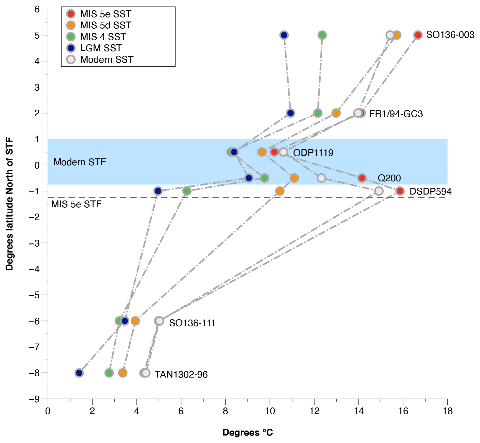
Figure 6 SST estimates from seven cores located in the southwestern Pacific. SST used were five-point averages (depending on sampling resolution) taken at MIS peaks and median dates in accordance with boundaries outlined in Lisiecki and Raymo (2005). Due to the complex circulation and frontal structures in the region, cores were plotted in ± distance from the average position of the modern STF. Cores used include SO136-003 (SSTs calculated from alkenones, Pelejero et al., 2006), FR1/94-GC3 (alkenones, Pelejero et al., 2006), ODP 181-1119 (PF-MAT, Hayward et al., 2008), DSDP594 (PF-MAT, Schaefer et al., 2005), Q200 (PF-MAT, Weaver et al., 1998), SO136-111 (D-MAT, Crosta et al., 2004), and TAN1302-96 (D-MAT; this study). The blue band represents the modern STF zone, while the red dotted line represents the southern shift in the STF during MIS 5e (Cortese et al., 2013).

4.4 Sea ice expansion and ocean circulation

Although the TAN1302-96 WSIC record suggests that sea ice was largely absent at the core site until the mid-glacial (∼65 ka), the observed changes in sea ice could have modulated regional fluctuations in Antarctic Intermediate Water (AAIW) subduction throughout the glacial–interglacial cycle. The annual growth and decay of Antarctic sea ice plays a critical role in regional water mass formation. Brine rejection results in net buoyancy loss in regions of sea ice formation, while subsequent melt results in freshwater inputs and net buoyancy gains near the ice margin (Shin et al., 2003; Pellichero et al., 2018). This increased freshwater input and buoyancy gain near the ice margin can hinder AAIW subduction, with direct and indirect impacts on both the upper and lower branches of the meridional overturning circulation (Pellichero et al., 2018).

Previous research has used δ¹³C in benthic foraminifera to track changes in the depth of the interface between AAIW and Upper Circumpolar Deep Water (UCDW) (Pahnke and Zahn, 2005; Ronge et al., 2015). Low δ¹³C values are linked to high nutrient concentrations found at depths below ∼1500 m in the UCDW, and higher δ¹³C values are associated with the shallower AAIW waters (Fig. 5). Marine sediment core MD97-2120 (45.535^∘ S, 174.9403^∘ E, core depth 1210 m) was retrieved from a water depth near the interface between the AAIW and UCDW water masses (Pahnke and Zahn, 2005). Over the last glacial–interglacial cycle, fluctuations in the benthic δ¹³C values from MD97-2120 suggest that the core site was intermittently bathed in AAIW and UCDW, and that the vertical extent of AAIW fluctuated throughout the last glacial–interglacial cycle. Ronge et al. (2015) used the δ¹³C values from MD97-2120 and other core sites to quantify the contributions of AAIW to the waters overlying MD97-2120 (%AAIW, Appendix D). These results suggest that during warm periods, MD97- 2120 exhibited more positive δ¹³C values, corresponding to higher %AAIW, while cooler periods exhibited more negative values, corresponding to lower %AAIW (Fig. 5). This suggests that during cooler periods, the AAIW-UCDW interface shoaled, reducing the total volume of AAIW and indirectly causing an expansion of UCDW (Ronge et al., 2015).

Our comparison between %AAIW and regional WSIC estimates suggest a strong link between the two (Fig. 5). Specifically, we observe that AAIW shoaled and UCDW expanded (i.e., %AAIW is low) during periods when sea ice expansion occurred. In contrast, during periods of low WSIC, a reduced seasonal sea ice cycle, and warmer summer sea surface temperatures (e.g., MIS 5e), %AAIW is observed to be high. This correlation supports the idea that increased concentrations of regional sea ice resulted in a substantial summer freshwater flux into the AAIW source region. This regional freshening likely promoted a shallower subduction of AAIW and a corresponding volumetric expansion of UCDW, which can be seen by the isotopic offset of the δ¹³C values between the reference cores, and also by the increased carbonate dissolution in MD97-2120 during glacial periods (Fig. 7) (Pahnke et al., 2003; Ronge et al., 2015). These findings directly link sea ice proxy records to observed changes in ocean circulation and water mass geometry.

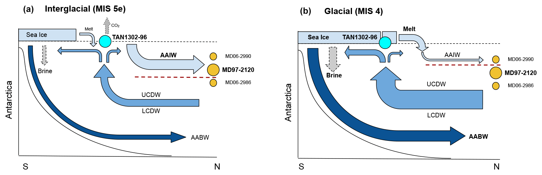
Figure 7 Schematic of changes in southwestern Pacific sector sea ice coverage and water mass geometry between interglacial and glacial stages. Panel (a) depicts interglacial conditions where sea ice coverage is minimal and freshwater input from summer sea ice melt is low. This lack of freshwater input allows AAIW to subduct to deeper depths and bath core MD97-2120, capturing the higher δ¹³C signature of the overlying AAIW waters. The AAIW-UCDW interface (red dashed line) is located beneath MD97-2120. CO₂ outgassing is occurring as a carbon-rich Circumpolar Deep Water upwell near Antarctica. Panel (b) depicts glacial conditions where sea ice expansion has occurred beyond TAN1302-96, increasing brine rejection, and stabilizing the water column. As a result of the increased sea ice growth, subsequent summer melt increases the freshwater flux into the AAIW source region and increases AAIW buoyancy. This buoyancy gain shoals the AAIW-UCDW interface above core MD97-2120, causing the core site to be bathed in low δ¹³C UCDW. The shoaling of AAIW causes an indirect expansion of CDW, increasing the glacial carbon stocks of the deep ocean, while sea ice reduces CO₂ outgassing via the capping mechanism.

In addition to its influence on regional freshwater forcing and AAIW reductions, these sea ice changes may also coincide with larger-scale deep ocean circulation changes. The most dramatic increases in winter sea ice observed in TAN1302-96 and SO136-111, along with changes in %AAIW, are initiated during MIS 4. These shifts also correspond to basin-wide changes in benthic δ¹³C values in the Atlantic Ocean that suggest a shoaling in the AMOC during MIS 4 (Oliver et al., 2010; Kohfeld and Chase, 2017). Changes in deep ocean circulation are also recorded in εNd isotope data in the Indian sector of the Southern Ocean (Wilson et al., 2015), suggesting extensive reductions in the AMOC during this period. Recent modelling literature (Marzocchi and Jansen, 2019; Stein et al., 2020) suggests that sea ice formation directly impacts marine carbon storage by increasing density stratification and reducing diapycnal mixing, especially in simulations where brine rejection is enhanced near the Antarctic continental slope and open ocean vertical mixing (and subsequent CO₂ outgassing) is reduced (Bouttes et al., 2010, 2012; Menviel et al., 2012). These simulations suggest a resulting CO₂ sequestration of 20–40 ppm into the deep ocean.

Taken collectively, the available data show that sea ice expansion, AAIW-UCDW shoaling, changes in the AMOC, and a decrease in atmospheric CO₂ all occur concomitantly during MIS 4 (Fig. 5). It appears likely, therefore, that sea ice expansion during this time influenced intermediate water density gradients through increased freshening and consequent shoaling of AAIW, which may also have increased the efficiency of the carbon pump and increased CO₂ uptake by phytoplankton (Sigman et al., 2021). This appears to have occurred while simultaneously influencing deep-ocean density, and therefore stratification, through brine rejection and enhanced deep water formation, which ultimately lead to decreased ventilation (Abernathey et al., 2016). These changes in ocean stratification, combined with the sea ice “capping” mechanism, appear to agree with both the recent modelling efforts (Stein et al., 2020) and observed proxy data and fit well within the hypothesis that mid-glacial CO₂ variability was primarily the result of a more sluggish overturning circulation (Kohfeld and Chase, 2017).

5 Summary and conclusion

This study presents new WSIC and SSST estimates from marine core TAN1302-96, located in the southwestern Pacific sector of the Southern Ocean. We find that the WSIC remained low during the early glacial cycle (130 to 70 ka), expanded during the middle glacial cycle (∼65 ka), and reached its maximum just prior to the LGM (∼24.5 ka). These results largely agree with nearby core SO136-111 but display some differences in WSIC magnitude with E27-23. This discrepancy may be explained by differences in statistical applications and/or lateral sediment redistribution, although more analysis is required to determine the exact cause(s).

The lack of changes in SSST and the absence of winter sea ice over the core site during the early glacial suggests that the sea ice capping mechanism and corresponding surface stratification in this region is an unlikely cause for early CO₂ drawdown, and that alternative hypotheses should be considered when evaluating the mechanism(s) responsible for the initial drawdown. More specifically, we consider the impact of changes in SSST gradients between ∼40 to 60^∘ S and support the idea that changes in air–sea disequilibrium associated with reduced sea-surface temperature gradients could be a potential mechanism that contributed to early glacial reductions in atmospheric CO₂ concentrations (Khatiwala et al., 2019). Another key consideration is the potentially non-linear response between sea ice expansion and CO₂ sequestration potential (i.e., that not all sea ice is equal in its capacity to sequester carbon). More analyses are required to adequately address this.

We also observe a strong link between regional sea ice concentrations and vertical fluctuations in the AAIW-UCDW interface. Regional sea ice expansion appears to coincide with the shoaling of AAIW, likely due to the freshwater flux from summer sea ice melt increasing buoyancy in the AAIW formation region. Furthermore, major sea ice expansion and AAIW shoaling occurs during the middle of the glacial cycle and is coincident with previously recognized shoaling in AMOC and mid-glacial atmospheric CO₂ reductions, suggesting a mechanistic link between sea ice and ocean circulation.

In conclusion, this paper has focused exclusively on sea ice as a driver of physical changes, but we recognize that these changes in sea ice will be accompanied by multiple processes that interact and compete with each other. Marzocchi and Jansen (2019) note that teasing apart the individual components of CO₂ fluctuations is complicated because of interactions between sea ice capping, air–sea disequilibrium, AABW formation rates, and the biological pump. We recognize that these processes may not act independently and, as such, have contributed new data to help advance our collective understanding of the role of sea ice on influencing atmospheric CO₂ variability on a glacial–interglacial timescale.

Appendix A: Age model and sampling depths

Table A1 Radiocarbon dates taken from TAN1302-96. NDFB = not distinguishable from the background.

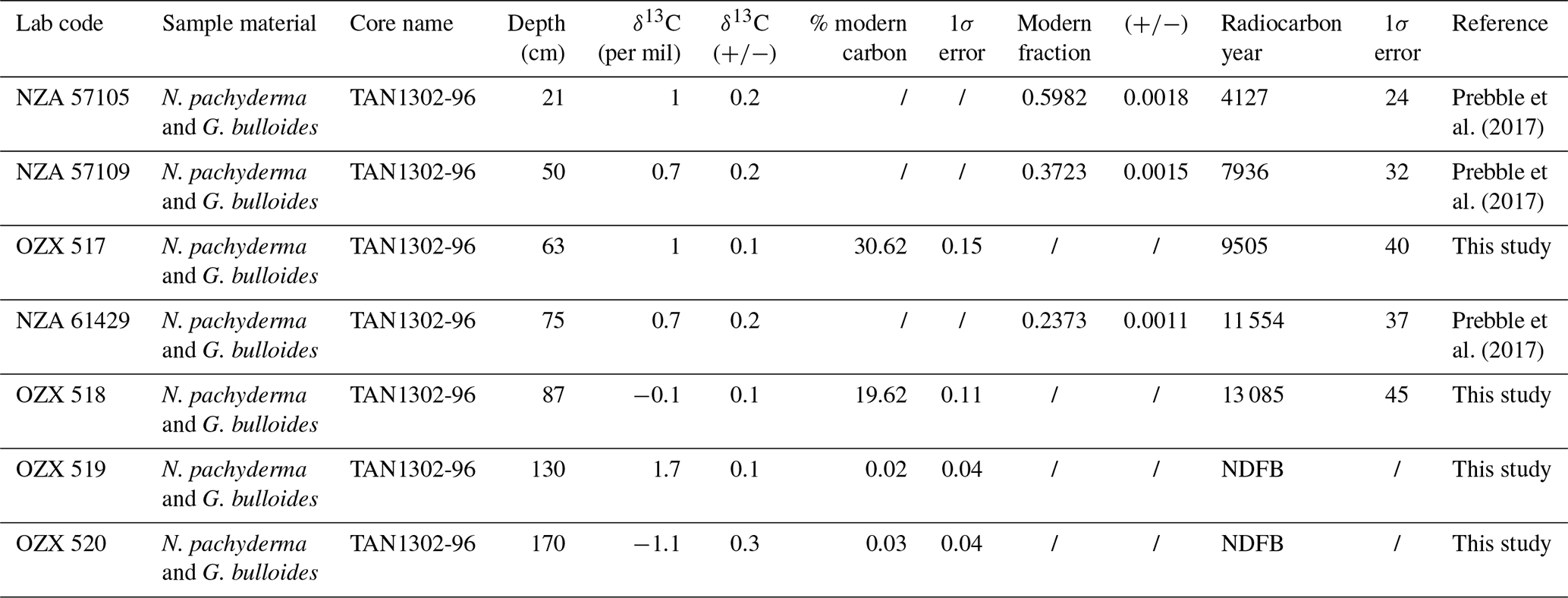
Table A2 Tie points used in construction of the TAN1302-96 age model.

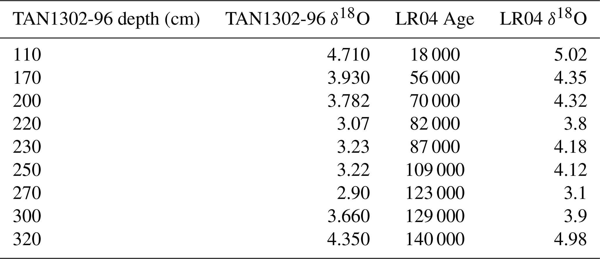
Table A3 Sample depth and corresponding age. Diatom slides using Method 1 used even-numbered sediment samples (e.g., 10, 20, 30), while diatom slides using Method 2 used odd-numbered sediment samples (e.g., 53, 87).

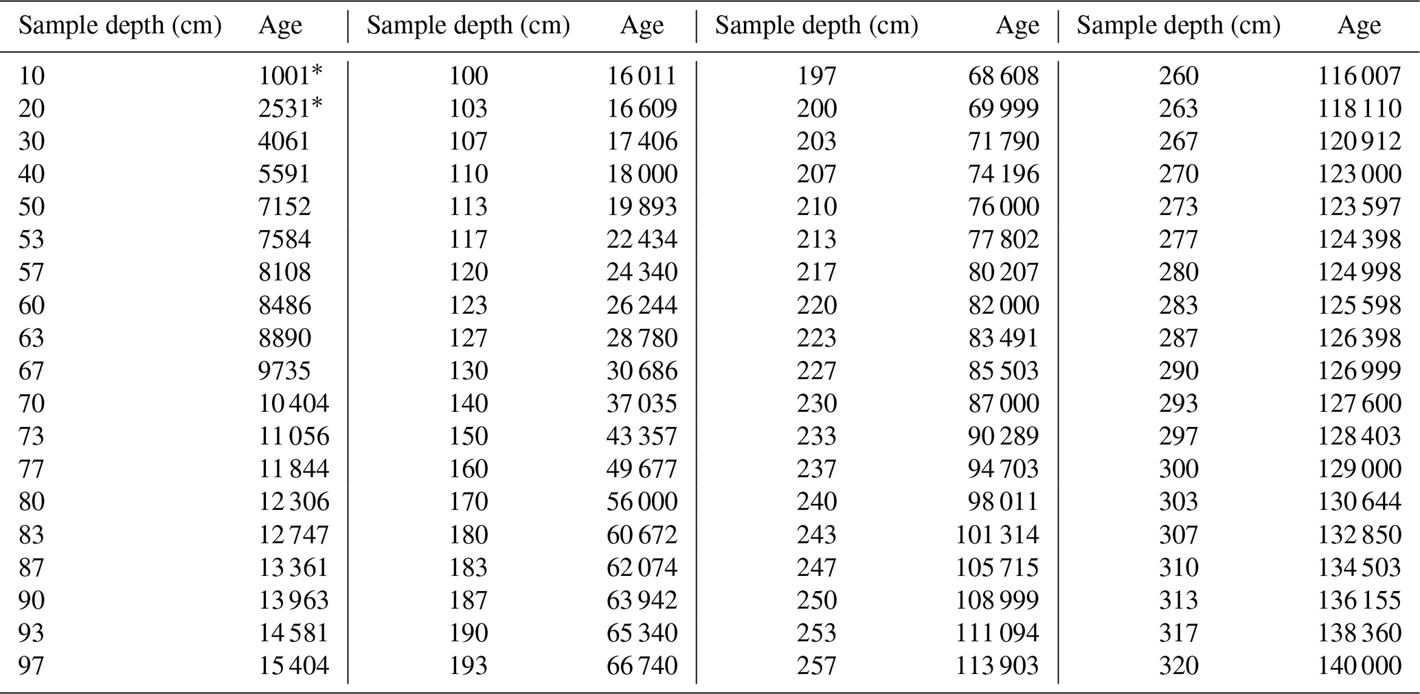
^* Indicates the sample was calculated based on linear sedimentation rates.

Appendix B: Diatom slide preparation comparison

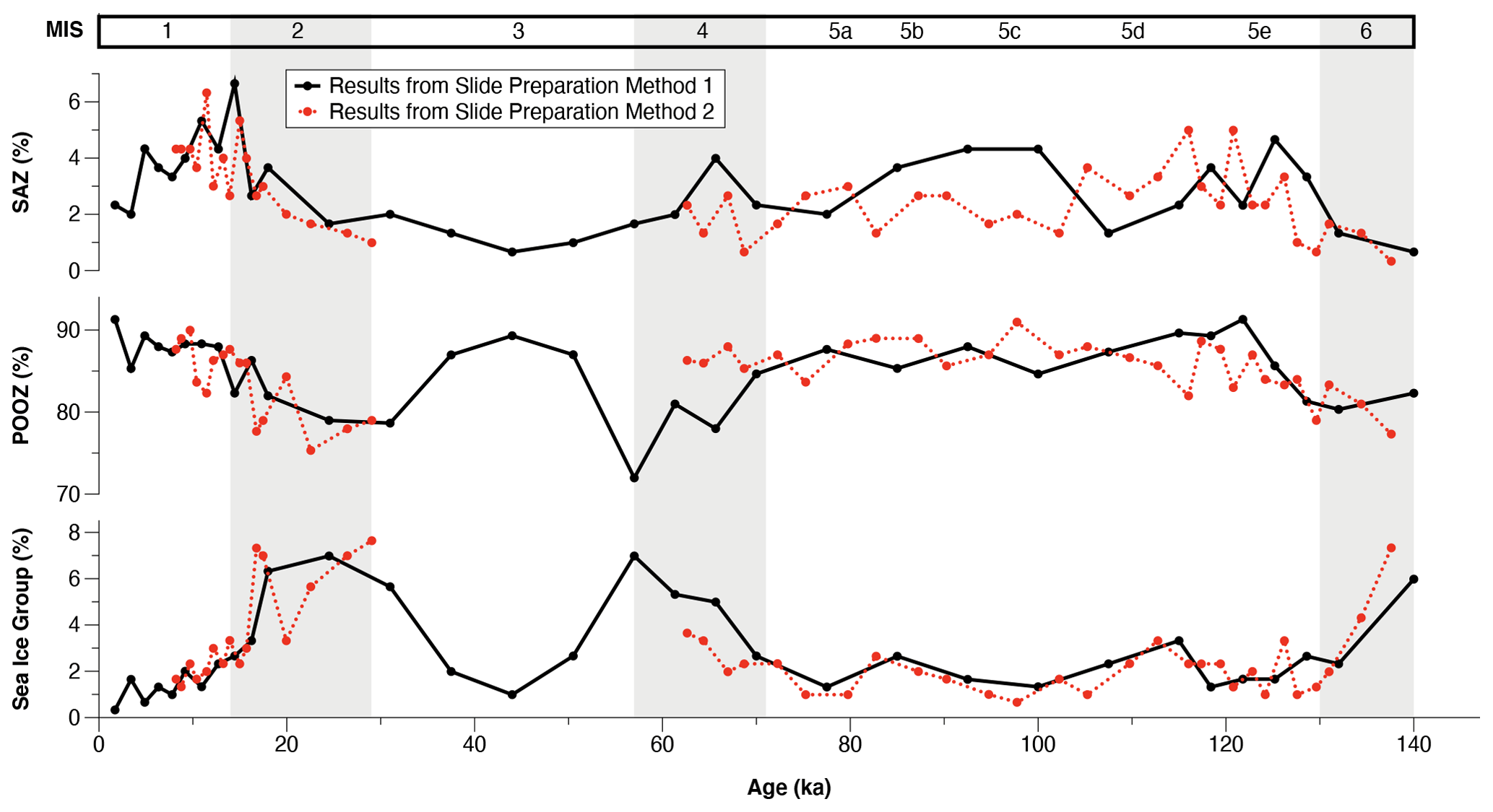
Figure B1 Results from diatom slide preparation methods 1 and 2. No notable differences or biases were observed between the two different methods.

Appendix C: TAN1302-96 and E27-23 comparison

Potential causes for WSIC estimate differences

The third potential cause for the observed differences between TAN1302-96 and E27-23 WSIC estimates is through the cumulative effects of different laboratory protocols. While it is difficult to determine precisely how much different laboratory protocols could influence the results, we cannot exclude this explanation as a possible contributor to differences in WSIC.

The fourth potential cause for differences in WSIC estimates between E27-23 and TAN1302-96 are differences in counting and identification methods. We believe this is an unlikely cause for the differences observed between E27-23 and TAN1302-96 primarily because of the magnitude of counting discrepancies required to cause a difference of 50 % WSIC estimates between the two cores. The close coupling of WSIC estimates between TAN1302-96 and SO136-111 over the entire glacial–interglacial cycle supports that a fundamental issue relating to taxonomic identification and/or methodology is an unlikely explanation for the observed WSIC differences.

Finally, the fifth potential cause of differing WSIC estimates is selective diatom preservation (e.g., Pichon et al., 1992; Ragueneau et al., 2000). The similarities between TAN1302-96 and SO136-111 WSIC estimates, along with independent indicators in cores E27-23 and TAN1302-96, suggest that this is unlikely. For E27-23, Bradtmiller et al. (2009) used the consistent relationship between ${}^{\mathrm{231}}\mathrm{Pa}{/}^{\mathrm{230}}\mathrm{Th}$ ratios and opal fluxes to suggest that dissolution remained relatively constant between the LGM and Holocene periods. In TAN1302-96, we assigned a semi-quantitative diatom preservation value between 1 (extreme dissolution) and 4 (virtually perfect preservation) for each counted specimen. The average preservation of diatoms for the entire core was 3.38±0.13, with no observed bias based on sedimentation rate or MIS. This assessment, although semi-qualitative, suggests that preservation remained relatively constant (and good) throughout TAN1302-96 and is therefore unlikely to cause large differences in WSIC between the two cores.

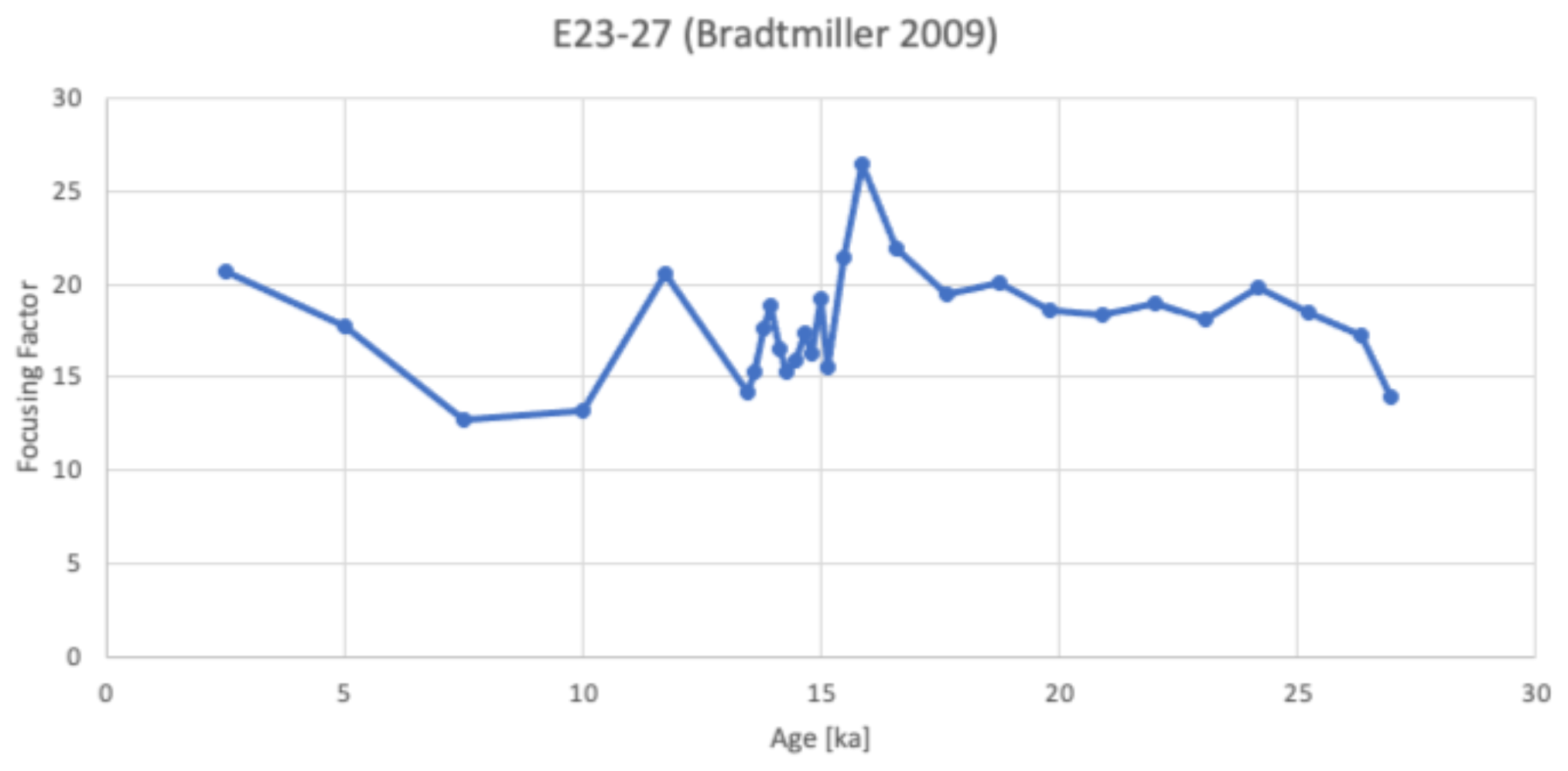
Figure C1 Preliminary focusing factor (FF) values for E27-23. These results suggest notable lateral sediment redistribution over the last 26 ka, requiring further analysis (Bradtmiller et al., 2009).

Appendix D: %AAIW calculation

The calculation of %AAIW in this study is the same as was used in Ronge et al. (2015):

$$\begin{array}{rl}\text{\%AAIW}=& \left({\mathit{\delta }}^{\mathrm{13}}{\mathrm{C}}_{\mathrm{MD}\mathrm{97}-\mathrm{2120}}-{\mathit{\delta }}^{\mathrm{13}}{\mathrm{C}}_{\mathrm{MD}\mathrm{06}-\mathrm{2986}}\right)/\\ & \left({\mathit{\delta }}^{\mathrm{13}}{\mathrm{C}}_{\mathrm{MD}\mathrm{06}-\mathrm{2990}}-{\mathit{\delta }}^{\mathrm{13}}{\mathrm{C}}_{\mathrm{MD}\mathrm{06}-\mathrm{2986}}\right)\times \mathrm{100}.\end{array}$$

All core information for MD97-2120, MD06-2986, and MD06-2990 can be found through the original publication.