the Creative Commons Attribution 4.0 License.
the Creative Commons Attribution 4.0 License.
 | 28 Feb 2022
Evolution of continental temperature seasonality from the Eocene greenhouse to the Oligocene icehouse –a model–data comparison
Agathe Toumoulin
Delphine Tardif
Yannick Donnadieu
Alexis Licht
Jean-Baptiste Ladant
Lutz Kunzmann
Guillaume Dupont-Nivet
At the junction of greenhouse and icehouse climate states, the Eocene–Oligocene Transition (EOT) is a key moment in Cenozoic climate history. While it is associated with severe extinctions and biodiversity turnovers on land, the role of terrestrial climate evolution remains poorly resolved, especially the associated changes in seasonality. Some paleobotanical and geochemical continental records in parts of the Northern Hemisphere suggest the EOT is associated with a marked cooling in winter, leading to the development of more pronounced seasons (i.e., an increase in the mean annual range of temperature, MATR). However, the MATR increase has been barely studied by climate models and large uncertainties remain on its origin, geographical extent and impact. In order to better understand and describe temperature seasonality changes between the middle Eocene and the early Oligocene, we use the Earth system model IPSL-CM5A2 and a set of simulations reconstructing the EOT through three major climate forcings: pCO2 decrease (1120, 840 and 560 ppm), the Antarctic ice-sheet (AIS) formation and the associated sea-level decrease. Our simulations suggest that pCO2 lowering alone is not sufficient to explain the seasonality evolution described by the data through the EOT but rather that the combined effects of pCO2, AIS formation and increased continentality provide the best data–model agreement. pCO2 decrease induces a zonal pattern with alternating increasing and decreasing seasonality bands particularly strong in the northern high latitudes (up to 8 ∘C MATR increase) due to sea-ice and surface albedo feedback. Conversely, the onset of the AIS is responsible for a more constant surface albedo yearly, which leads to a strong decrease in seasonality in the southern midlatitudes to high latitudes ( S). Finally, continental areas that emerged due to the sea-level lowering cause the largest increase in seasonality and explain most of the global heterogeneity in MATR changes (ΔMATR) patterns. The ΔMATR patterns we reconstruct are generally consistent with the variability of the EOT biotic crisis intensity across the Northern Hemisphere and provide insights on their underlying mechanisms.
- Article
(10992 KB) - Full-text XML
-
Supplement
(4549 KB) - BibTeX
- EndNote


1.1 Context and aim of the study
The Eocene–Oligocene Transition (EOT) is marked by an abrupt cooling event (∼2.9 ∘C from marine proxies; Hutchinson et al., 2021), regarded as the hinge between the Eocene greenhouse and the later Cenozoic icehouse. This event is associated with the first major expansion of the Antarctic ice sheet with an estimated sea-level drop of ∼70 m (Hutchinson et al., 2021; Miller et al., 2020). The EOT is described as a relatively brief event (∼790 000 years), with two successive steps (at ca. 33.9 and 33.7) recognized in extensively studied marine environments, especially from deep ocean δ18O values (e.g., Katz et al., 2008; Zachos et al., 2001; see the review of Hutchinson et al., 2021).
Reported vegetation responses to the EOT appear to be heterogeneous across continents with important composition changes in some areas (e.g., the west coast of the United States, Greenland, Asia), notably where faunal turnover is important (e.g., Barbolini et al., 2020; Hutchinson et al., 2021; Pound and Salzmann, 2017; Wolfe, 1994). A number of paleobotanical and geochemical studies consistently suggest that the decrease in continental temperatures was particularly marked during winter months, thus leading to higher seasonal temperature contrasts, which are designated as a potential driving mechanism for biotic turnovers (e.g., Eldrett et al., 2009; Mosbrugger et al., 2005; Page et al., 2020; Utescher et al., 2015; Zanazzi et al., 2015). Evoked forcing mechanisms explaining this enhanced winter cooling are pCO2, Antarctic ice-sheet (AIS) inception and increased continentality, although it remains difficult to quantify and disentangle their respective contribution from field data only. Understanding the drivers of these seasonal changes is thus important, not only for assessing the climate system behavior under major pCO2 variations but also to better describe the paleoenvironmental context associated with major extinction events of the EOT such as the Grande Coupure in Europe and the Mongolian Remodeling in central Asia (Meng and McKenna, 1998; Stehlin, 1909; see Coxall and Pearson, 2007, for a review).
By comparing paleoclimate simulations to a synthesis of indicators of seasonality changes (Table S1 in the Supplement), our study attempts to retrieve the evolution of seasonal temperature contrast from the middle Eocene to the early Oligocene. The EOT is reconstructed step by step from five simulations, describing the evolution of three major forcings of this time: the pCO2 drawdown, the AIS expansion and the resulting sea-level lowering, in order to understand the respective contribution of each component to the resulting seasonality change patterns, along with their possible synergies and retroactions.
1.2 Temperature seasonality and its evolution
Temperature seasonality can be quantified by the mean annual temperature range (MATR), which consists of the temperature difference between the warmest and coldest months of the year. Increasing MATR can occur through increased summer temperatures, lowered winter temperatures or both. MATR is practical because it can be directly calculated from temperature proxies providing an estimation of the lowest and highest temperatures within a year. This is the case for the Climate Leaf Analysis Multivariate Program (CLAMP), which reconstructs temperatures from the modern correlation between climate variables and leaf physiognomy (Wolfe, 1993; Yang et al., 2011), or the Coexistence Approach (CA), which uses modern relatives of fossil species to define a mutual climate range of environmental characteristics (Grimm and Potts, 2016; Mosbrugger and Utescher, 1997; Utescher et al., 2014). MATR can also be deduced from the variability of the temperature signal in geochemical proxies for temperatures, stable oxygen isotopes (δ18O), as the time resolution of the proxy rarely allows for the direct reconstruction of seasonal temperatures (e.g., Ivany et al., 2000; Wade et al., 2012).
The spatial distribution of temperature seasonality changes across the EOT appears to be heterogeneous in proxy data (e.g., Pound and Salzmann, 2017). Most changes are described in the Northern Hemisphere from paleobotanical reconstructions and converge to show seasonalities stronger in the early Oligocene than in the mid- to late Eocene. In North America, western and central Europe, seasonality increase is recorded by the decline in species characteristic of warm paratropical to temperate environments such as palms (e.g., Nypa sp.), plants from the myrtle and eucalyptus family (Myrtaceae, e.g., Rhodomyrtophyllum sp.), conifers (e.g., Doliostrobus sp.) and some plant families with tropical elements (e.g., Annonaceae, Lauraceae, Cornaceae, Icacinaceae, Menispermaceae), and, depending on the bioclimatic zones, the expansion of temperate to boreal vegetation through the increase in deciduous and/or coniferous species (Kunzmann et al., 2016; Kvaček, 2010; Kvaček et al., 2014; Mosbrugger et al., 2005; Utescher et al., 2015; Wolfe, 1992). These vegetation changes are associated with a decrease in the coldest month mean temperature (CMMT) across the EOT and start before the EOT at some localities, during the mid- to late Eocene (Moraweck et al., 2019; Mosbrugger et al., 2005; Tanrattana et al., 2020; Tosal et al., 2019; Utescher et al., 2015; Wolfe, 1994). Isotopic analyses have documented this seasonality increase in different continental localities between the Priabonian (37.8 to 33.9 Ma) and the Rupelian (33.9 to 27.82 Ma; Grimes et al., 2005; Hren et al., 2013; Zanazzi et al., 2015). While some of the changes are not directly quantifiable (e.g., the reduction in gastropod growing season length, United Kingdom; Hren et al., 2013; dental morphological changes for grazing perissodactyls, Europe; Joomun et al., 2010), others can demonstrate strong MATR increase (e.g., amplified by 15.6 ∘C, Canada; Zanazzi et al., 2015). A temperature seasonality increase is also documented for shallow waters of the Gulf of Mexico (increase in the MATR; Ivany et al., 2000; Wade et al., 2012). Some studies have suggested a link between increased temperature seasonality and latitude (e.g., Zanazzi et al., 2007, 2015), but data seem insufficient to validate this relationship, and this trend has not been confirmed by recent palynological compilation (Pound and Salzmann, 2017).
Data from southeast Europe and Anatolia show generally weaker and heterogeneous changes in temperature seasonality, with either no seasonality changes, slight seasonality lowering or slight seasonality strengthening from the mid-Eocene to the Rupelian (Bozukov et al., 2009; Kayseri-Özer, 2013). This variability has been explained by a strong marine influence on this part of Eocene Europe (Kayseri-Özer, 2013). Conversely, north and East Asia temperature seasonality evolution is more comparable to western Europe and North America trends (Quan et al., 2012; Utescher et al., 2015). Vegetation changes reflect an increase in the seasonal temperature range, mainly through the EOT (MATR increase of 2 to 2.5 ∘C; CMMT decrease of ∼2.2 ∘C, Quan et al., 2012; Utescher et al., 2015). The appearance of tubers in lotus (Nelumbo sp.) during the Eocene suggests the establishment of a dormant phase in these plants and thus of a period unfavorable to plant growth (Li et al., 2014). Fossils showing these structures have been described in southern China (Hainan Province) and easternmost Russia (Kamchatka Peninsula) leading to the hypothesis that they could be favored by cooling and increased seasonality on the East Asian continent during the Eocene (Budantsev, 1997; Li et al., 2014).
In the Southern Hemisphere, studies of Paleogene localities are rarer. Despite a record of late Eocene cooling in Australia, New Zealand and Patagonia, independent proxies (stable isotopes on teeth, bones and pedogenic carbonates, paleobotanical reconstructions) do not suggest a marked temperature seasonality during the Eocene (Colwyn and Hren, 2019; Kohn et al., 2015; Lauretano et al., 2021; Nott and Owen, 1992; Pocknall, 1989). In Australia, the presence of more pronounced tree rings suggests a late Paleogene increase in seasonality starting in the mid-Oligocene at the earliest (Bishop and Bamber, 1985; Nott and Owen, 1992). Finally, the environmental and climatic impact of the EOT in continental Africa remains poorly documented (Hutchinson et al., 2021; Saarinen et al., 2020).
1.3 Previous model work
Different modeling studies have illustrated the priming role of pCO2 lowering during the EOT, but most focused on oceans through mean annual temperature changes (Baatsen et al., 2020; Goldner et al., 2014; Hutchinson et al., 2018, 2021; Kennedy et al., 2015; Kennedy-Asser et al., 2019, 2020; Ladant et al., 2014b). The model intercomparison study of Hutchinson et al. (2021) has shown a reasonable agreement between modeling experiments with 1120 and 560 ppm (i.e., 4 and 2 times the preindustrial atmospheric levels, respectively, with 1 PAL = 280 ppm and hereafter written “4X” and “2X”) and proxy-data atmospheric and surface ocean temperature reconstructions from the late Eocene and the early Oligocene, respectively. They show, however, that changes in EOT sea surface temperatures (SSTs) were on average best represented by a pCO2 shift from 910 to 560 ppm (i.e., a drop of 1.6X). In addition, a recent model–data study of Lauretano et al. (2021) explored Australia climate evolution through the EOT, and estimated a pCO2 drop ranging from 260 to 380 ppm (drop of ∼0.9–1.3X). A first attempt to explain temperature seasonality change across the EOT was made by Eldrett et al. (2009). In their palynological and modeling study, Eldrett and coauthors explained high-latitude (Greenland) seasonality strengthening by pCO2 drop and the consequent increase in sea-ice formation over the Arctic Ocean. In their experiment, sea-ice extension induces a strong albedo feedback, which results in a large decrease in atmospheric temperature during winter. Additionally, changes in geography (topography, land–sea distribution) may have significant effects on terrestrial temperatures at a regional scale (e.g., Lunt et al., 2016; Li et al., 2018). EOT modeling experiments yield mixed answers regarding the temperature feedback resulting from both AIS and contemporary paleogeographic changes (opening of Southern Ocean gateways, Antarctic geography or global geography; Goldner et al., 2014; Hutchinson et al., 2021; Kennedy et al., 2015; Ladant et al., 2014a, b). The few studies testing the combined effect of both AIS and paleogeographic changes (Kennedy et al., 2015; Lauretano et al., 2021) suggested a moderate impact of AIS on global climate sensitivity, as previously suggested by other modeling work (Goldner et al., 2013; Kennedy et al., 2015).
2.1 Model and simulation setting
We used the IPSL-CM5A2 general circulation model, which is built upon the CMIP5 Earth system model developed at the Institut Pierre-Simon Laplace (IPSL), i.e., IPSL-CM5A-LR (Dufresne et al., 2013; Sepulchre et al., 2020). The IPSL-CM5A-LR Earth system model is composed of the LMDZ atmospheric model (Hourdin et al., 2013), the ORCHIDEE land surface and vegetation model (Krinner et al., 2005), and the NEMO v3.6 ocean model which includes modules for ocean dynamics (OPA8.2; Madec, 2016), biochemistry (PISCES; Aumont et al., 2015) and sea ice (LIM2; Fichefet and Morales-Maqueda, 1997). The atmospheric grid has a horizontal resolution of 3.75∘ longitude per 1.875∘ latitude (96×95 grid points) and is divided into 39 vertical levels. For a more detailed description of the model and its different components, the reader is referred to Sepulchre et al. (2020).
Five simulations were carried out to reconstruct the evolution of temperature seasonality from the middle Eocene to the early Oligocene (Table 1). The applied 40 Ma paleogeography framework is the map developed by Poblete et al. (2021) and already used in Tardif et al. (2020) and Toumoulin et al. (2020). It features common late Eocene geography characteristics such as an open Panama Seaway, an open Tethys with a submerged Arabian Peninsula, a strongly maritime Europe, a Turgai land bridge connecting northern Europe with Asia and narrow Southern Ocean gateways (Fig. 1). The orbital parameters were set to preindustrial values and the solar constant was reduced accordingly to its Eocene value (1360.19 W m−2; Gough, 1981). Vegetation was implemented as a boundary condition, using a zonal band of PFTs using modern vegetation distribution patterns.
Table 1Experimental design. Abbreviations: AIS – Antarctic ice-sheet volume (Ladant et al., 2014b); %Land – total land surface (millions of square kilometers – 106 km2); MAT – mean annual global 2 m air temperature (∘C); SST – sea surface temperature (∘C). Simulations with an asterisk constitute realistic middle Eocene (Lutetian/Bartonian) and early Oligocene (Rupelian) scenarios; others are either sensitivity experiments (2X, 2X-ICE) or use the high value of the pCO2 range estimated for the time interval (4X).


Figure 1Paleotopographic 40 Ma map: (a) standard version as used for simulations 4X, 3X, 2X and 2X-ICE; (b) version adjusted with a homogeneous 70 m sea-level lowering used for the simulation 2X-ICE-SL (Poblete et al., 2021).
Simulations were compared in pairs to highlight differences between the middle/late Eocene and the early Oligocene. The simulation set is composed of both realistic and idealized experiments (Table 1). Simulations 4X, 3X and 2X represent most of the pCO2 range described from the mid-Eocene (Lutetian) to the early Oligocene (Rupelian; Foster et al., 2017). These pCO2 values enable the description of the pCO2 reduction effect on climate through this time interval and have been used in most previous modeling experiments on the EOT (Hutchinson et al., 2021). Simulations 4X and 3X cover the range of potential climate values prior to the EOT (Lutetian to Priabonian). The idealized simulation 2X allows the identification of a 1 to 2 PAL pCO2 lowering alone. In a complementary way, simulations 2X-ICE and 2X-ICE-SL describe the early Oligocene climate, following the Antarctic ice-sheet formation. Both simulations are parameterized in the same way apart from the sea level, which is 70 m lower in 2X-ICE-SL. The use of 2X-ICE provides a theoretical description of the effect of an ice-covered Antarctica on climate, while 2X-ICE-SL constitutes a more realistic representation of the early Oligocene climate. In these experiments, the Antarctic ice cap was set to 32.5× 10⁶ km3 according to Ladant et al. (2014b). The 70 m sea-level drop was defined following eustatic drop estimates for the EOT (Coxall et al., 2005; Katz et al., 2008; Lear et al., 2008; Miller et al., 2020). It is responsible for important geography changes related to an increase in land proportion, such as the emergence of the Arabian Peninsula and the retreat of the proto-Paratethys epicontinental sea.
All simulations run for 4000 years until temperatures indicate a quasi-equilibrium with only negligible temperature drift within the global mean ocean (<0.1 ∘C per century; Fig. S1 in the Supplement). These trends are consistent with most model studies and do not affect the quality of atmospheric change described in this study (e.g., Hutchinson et al., 2018; Lunt et al., 2016). The results considered here are averages of the last 100 years of the model runs.
2.2 Data compilation
Simulation results were compared to MATR changes (ΔMATR) documented by proxy-data records (Table S1 in the Supplement). We compiled published MATR and CMMT proxy data from various research fields: paleobotany (macrofossils and palynology), geochemistry (isotopic measurements on various material) and paleontology. The data were selected to range from the Lutetian (47.8 Ma) to the end of the Rupelian (27.8 Ma). This large time interval allows the representation of seasonal temperature changes parallel to the long-term cooling of the Eocene. The inclusion of data from the middle Eocene allows a comparison with simulations testing the effect of a pCO2 lowering alone, before AIS formation at the EOT. It is justified by the presence of paleobotanical records suggesting a strengthening of the seasons already from the Lutetian to the Priabonian (e.g., Li et al., 2014; Mosbrugger et al., 2005). Compiled Eocene–Oligocene ΔMATRs correspond either to the values given in original publications, when they were available and precise, or to values recalculated from the original data. For publications for which ΔMATRs were recalculated, we proceeded by grouping the closest sites (especially in terms of latitudes) and checked that the values obtained were consistent with the authors' original interpretation of the paleoenvironmental context. Half of the data come from the pollen compilation of Pound and Salzmann (2017). A selection was made through this study data to keep (1) the best-dated samples, according to their dating quality indicator (data Q1 to Q3; Pound and Salzmann, 2017), and (2) sites with temperature estimates for the Priabonian and Rupelian or at least one nearby locality that could be compared. No Eocene–Oligocene site was selected for more clarity. In an effort to limit the addition of overly uncertain ΔMATR data, sites with a range of CMMT estimates (CMMTmax–CMMTmin) ≥10 ∘C (either for Priabonian or Rupelian sites) were excluded.
Some previously published seasonality increases were not associated with estimates of ΔMATR because seasonality strengthening was either (1) suggested from other parameters, such as the length of the growing season, which does not allow the calculation of the MATR (Hren et al., 2013), or (2) derived from qualitative data that cannot be specifically associated with temperature values (e.g., morphological changes such as tooth shape or plant tuber appearance; Joomun et al., 2010; Li et al., 2014). These sites are displayed on the maps in orange but are not included in quantitative analyses (Sect. 2.3). In order to better estimate the impact of changes in temperature seasonality, the length of the plant growing season (i.e., the number of months with an average temperature above 10 ∘C) was recalculated using the formula of Grein et al. (2013) for Coexistence Approach data (Table 1). Paleocoordinates for every locality were reconstructed using the online service of Gplates (https://www.gplates.org/, last access: 16 February 2022), according to the 40 Ma paleogeography used for the paleoclimate models (Poblete et al., 2021) that essentially follows the plate tectonic reconstruction model of Matthews et al. (2016) with some modifications.
2.3 Comparison of model and data ΔMATR
Different analyses were made to evaluate the data–model agreement for temperature seasonality changes from the Priabonian to Rupelian (Table 2). Modeled ΔMATR values were extracted from a 3∘ longitude by 3∘ latitude area surrounding each data locality. First, a general agreement percentage was calculated from the direction of seasonality changes alone to assert the agreement between our simulation and qualitative data. For this metric, model predictions are considered “good” for an individual site if the modeled ΔMATR changes in the same direction as the data (i.e., if a modeled ΔMATR increases/decreases at the location of a data point showing seasonality increase/decrease). For data indicating null ΔMATR, good agreement was considered to exist when model values ranged from −0.5 to 0.5 ∘C.
In addition, Priabonian to Rupelian seasonality changes were compared to model predictions, by (1) testing their correlation and (2) calculating the root of the mean squared distance between their values. These two analyses were performed using R (version 4.0.3; R CoreTeam, 2020, Boston, USA). Given the limited number of quantitative Priabonian–Rupelian data (n=29), the statistical correlation of data–model ΔMATR was assessed from average ΔMATR with the non-parametric Spearman rank test. In this analysis, we used the common significance level, α, of 0.05 (i.e., p values <0.05 indicate significant correlations). The root mean squared estimate consists of calculating the root of the mean squared distance between model and data values for comparable points (RMSE; see Kennedy-Asser et al., 2020, and their Fig. S1 in the Supplement for a detailed presentation of the method). Conversely to the Spearman rank test, for which mean ΔMATR estimations were used, the distance is here measured using the full range of estimates at each data locality (i.e., minimum and maximum ΔMATR). Note that, because it considers the full range of ΔMATR, this method tends to minimize the difference between model and data. The lower bound of modeled ΔMATR at each locality was calculated as the difference between the lowest MATR value over the area centered around the locality for an Oligocene-like cold simulation (2X, 2X-ICE or 2X-ICE-SL) and the highest MATR value over the area for an Eocene simulation (4X or 3X). For the upper bound, we used the difference between the higher MATR value over the same area for an Oligocene-like cold simulation and the lower MATR value for an Eocene simulation.
The RMSE adjusted to ΔMATR is written as follows:
where ΔMATRdata and ΔMATRmodel are MATR Priabonian to Rupelian changes estimated by data and model, respectively, and n is the total number of localities.
3.1 Simulated response to pCO2 lowering
In this section, we compare the simulations 4X, 3X and 2X together to describe the effects of pCO2 drawdown on climate and provide a range of possible MAT and MATR change intensities. The simulation pair 2X–4X represents the strongest possible changes, 3X–4X the weakest changes and 2X–3X an intermediate scenario (see Sect. 2.1). Mean annual temperatures decrease strongly in our different experiments (Table 1, Fig. 2). The halving of pCO2 from 4X to 2X alone (i.e., without AIS formation and sea-level drop) induces a global cooling of 5.8 and 5.0 ∘C for the air temperature and the surface ocean, respectively (Table 1). A pCO2 drop of 1 PAL induces a 2.7 to 3.1 ∘C lowering of MAT and a 2.3 to 2.7 ∘C cooling of the SST, for 4X to 3X and 3X to 2X changes, respectively. Along with its effect on annual temperatures and regardless of its intensity, pCO2 decrease induces zonal ΔMATR including (1) an increase in MATR at high latitudes (especially in the north), (2) a decrease in MATR across most midlatitudes and (3) moderate changes at low latitudes, which we detail in the following Sects. 3.1.2 and 3.1.3 (for Eocene MATR values, see Fig. S2).
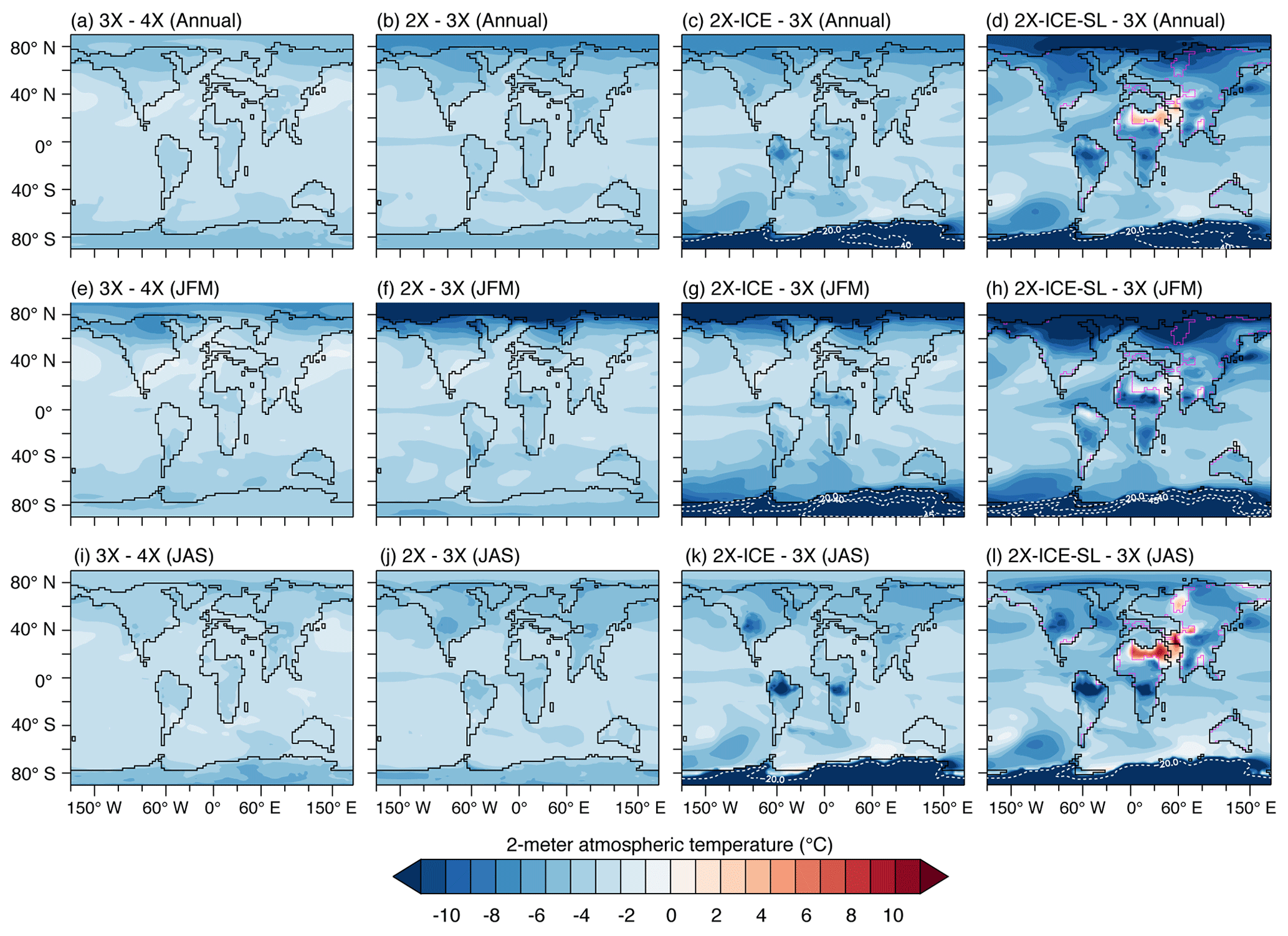
Figure 2Two-meter air temperature changes ( ∘C). JFM: averaged over January to March; JAS: averaged over July to September. Magenta lines of (d), (h) and (l) indicate shorelines before sea-level lowering. White dotted lines in (c), (d), (g), (h), (k) and (l) are the level lines encircling the 20, 40 and 45 ∘C cooling zones.
3.1.1 Areas with increased seasonality
Temperature changes are characterized by polar amplification, with a stronger winter cooling at high latitudes (Fig. 2a, b, e, f, i and j), likely due to the combined effect of albedo and sea-ice feedback. Below a given threshold (situated between 2 and 3 PAL), the pCO2 drop enables sea-ice growth over the Arctic and, to a lesser extent, the subsistence of snow on the ground during the cold season, which increases winter surface albedo (Fig. 3). In addition, seasonal sea-ice expansion limits ocean-to-air heat transfer at the highest northern latitudes and contributes to further winter cooling of the atmosphere. This preferential lowering of winter temperatures results in a large MATR increase of 5–20 % (3X–4X and 2X–3X) and up to 40 % (2X–4X; Figs. 4e and S3b) over high northern latitudes. Furthermore, the areas of colder winters and high MATR widen as pCO2 decreases: MATR increases from 60∘ N poleward between 4X and 3X, to 50∘ N poleward between 4X and 2X (Figs. 4 and S4). In contrast, Antarctica shows moderate ΔMATR (regionally up to 3 ∘C from 4X to 3X and 6 ∘C from 3X to 2X) compared to high northern latitude lands (6 ∘C MATR increase from 4X to 3X and 10 ∘C from 3X to 2X). This is because Antarctica is characterized by high MATR values in all ice-sheet-free experiments (4X, 3X and 2X), resulting in low ΔMATR changes from one experiment to another (Fig. 4a and b). This important seasonality is induced by the continent's high albedo variability, as it oscillates from snow-free to snow-covered soil within a year.
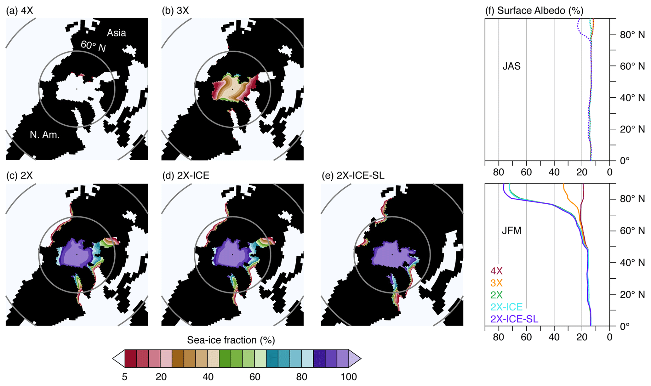
Figure 3Northern Hemisphere winter sea-ice fraction and surface albedo (%).
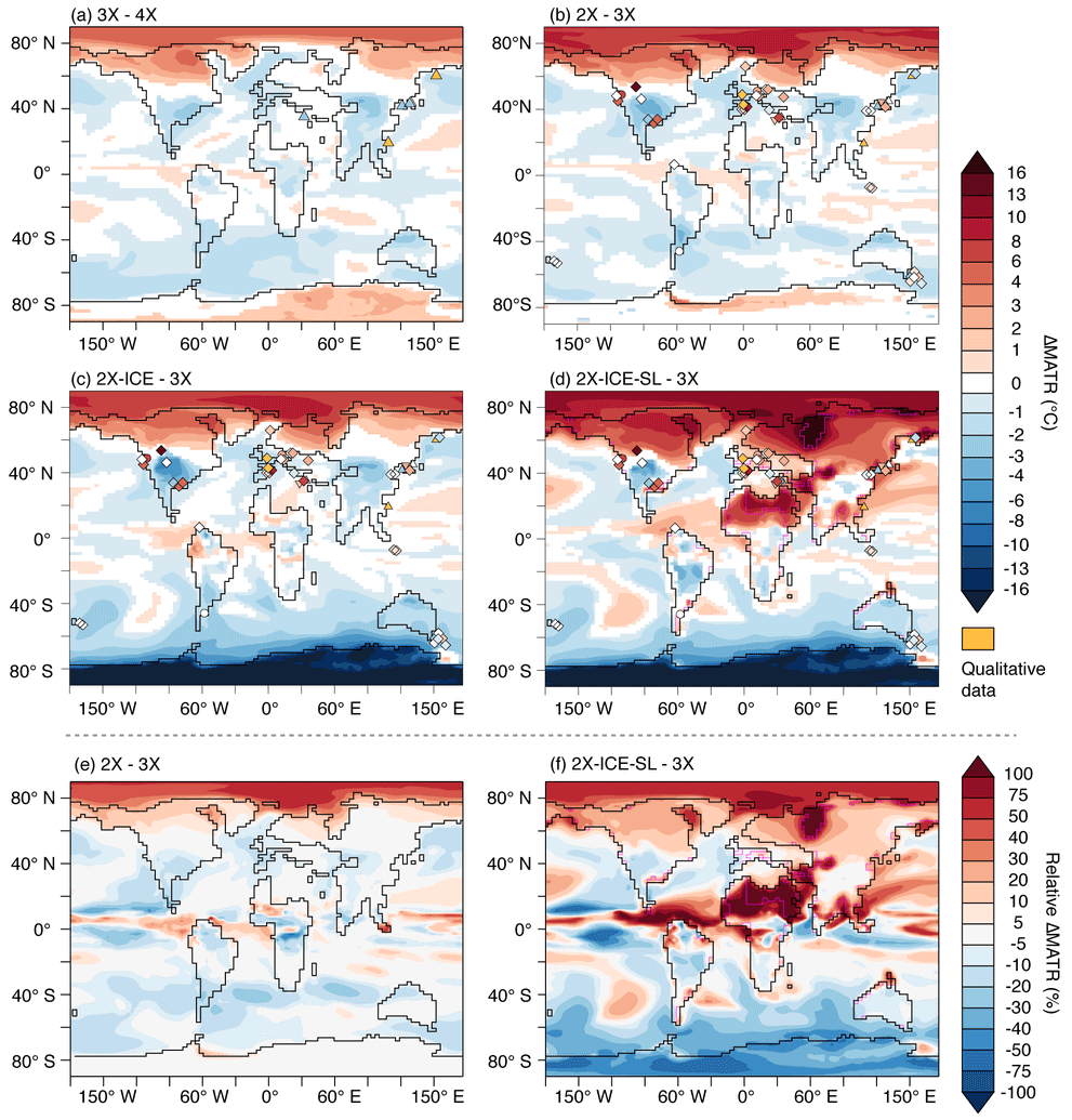
Figure 4Changes in mean annual temperature range, ΔMATR (∘C). Shadings are model differences calculated with a Student t test over the last 100 years of comparative simulations (95 % confidence); white areas indicate no significant ΔMATR. Panels (e) and (f) indicate relative ΔMATR (in %) for 2X–3X and 2X-ICE-SL–3X, respectively. Symbols correspond to ΔMATR from proxy data for different time steps: Priabonian–Lutetian (triangles); Rupelian–Lutetian (inverted triangles); Rupelian–Bartonian (circles); Rupelian–Priabonian (diamonds). Orange symbols indicate qualitative values describing a temperature seasonality increase. In the case of proxies reconstructing a range of equally probable values (e.g., the Coexistence Approach), the values shown are mean values. References are displayed in Fig. 8 and available in the data compilation provided in Table S1 in the Supplement.
3.1.2 Areas with decreased seasonality
Areas with decreased seasonality are characterized by summer cooling that exceeds winter cooling, which reduces the MATR (Figs. 2 and 4). The widest zones of decreasing MATR are continental regions located within the 30–50∘ latitudinal band. The magnitude of simulated MATR reduction depends on the pCO2 drop considered, with a reduction from 3X to 2X and from 4X to 2X resulting in up to 20 % and 30 % of regional MATR decrease, respectively (Figs. 4 and S3). At lower latitudes, in Amazonia, equatorial Africa and India, seasonality decreases but to a lesser extent (Fig. 4). A variety of atmospheric and oceanic processes are likely involved in these contrasting MATR changes, depending on the region considered.
The good correlation between MATR increase (respectively, decrease) and net precipitation decrease (respectively, increase; i.e., North America, Central Asia and northern Australia) suggests a strong involvement of the hydrological cycle in this phenomenon (Figs. 5 and 6a, c and h). The pCO2 drop tends to slow down the hydrological cycle, which results in flatter latitudinal gradients. At high latitudes, a reduction in precipitation leads to an overall decrease, while at midlatitudes to low latitudes, increased precipitation results in a general increase (Figs. 5 and 6). In these low-latitude to midlatitude zones, precipitation strengthening is more important in summer and associated with increased evaporation, which results in larger latent heat fluxes and thus in a greater cooling during summer, consistently with decreased seasonality (Fig. 6a, c, h). In addition, summer cooling is strengthened through vegetation feedback: increase favors net primary productivity which in turn contributes to evaporation and summer warmth loss (Fig. 6a, c, h). In contrast, decreased MATR in Europe and southern South America appears poorly correlated to the above-mentioned parameters (Fig. 6b and g). For Europe, the presence of sea ice over the Arctic Ocean (Fig. 3b–e) limits heat loss via the atmosphere during winter and results in a greater summer cooling of the SST (Fig. S5), which contributes to lowering European MATR. In addition, a regional increase in low-level cloud cover during summer could also contribute to lowering MATR for both Europe and southern South America through albedo feedback (5 % to 15 % higher low-level cloud fraction between 40–60∘; Figs. 7 and S6). For southern South America, several parameters seem consistent with the MATR reduction, but it is difficult to disentangle their contribution. By amplifying the latitudinal temperature gradients, the pCO2 drop induces a northward migration of the westerly wind maximum (by about 2∘ of latitude annually but less markedly during austral winter, JAS) and of the Antarctic Circumpolar Current, which delimits the Southern Hemisphere subpolar and subtropical gyres. This northward shift limits the arrival of warm subtropical waters near the poles (Fig. S7). This greater cooling in summer SST reinforces the ocean's buffering effect on atmospheric temperatures in southern South America and favors milder summers, and to a lesser extent, cooler winters, which is consistent with a decrease in seasonality (Figs. 4 and 7). Finally, changes in atmospheric dynamics (decrease in the width and increase in the intensity of the Hadley cell) are also visible and could have an impact on air–ocean exchanges, but much more analysis would be needed to understand their implication, which is not the focus of this paper (Fig. S8).
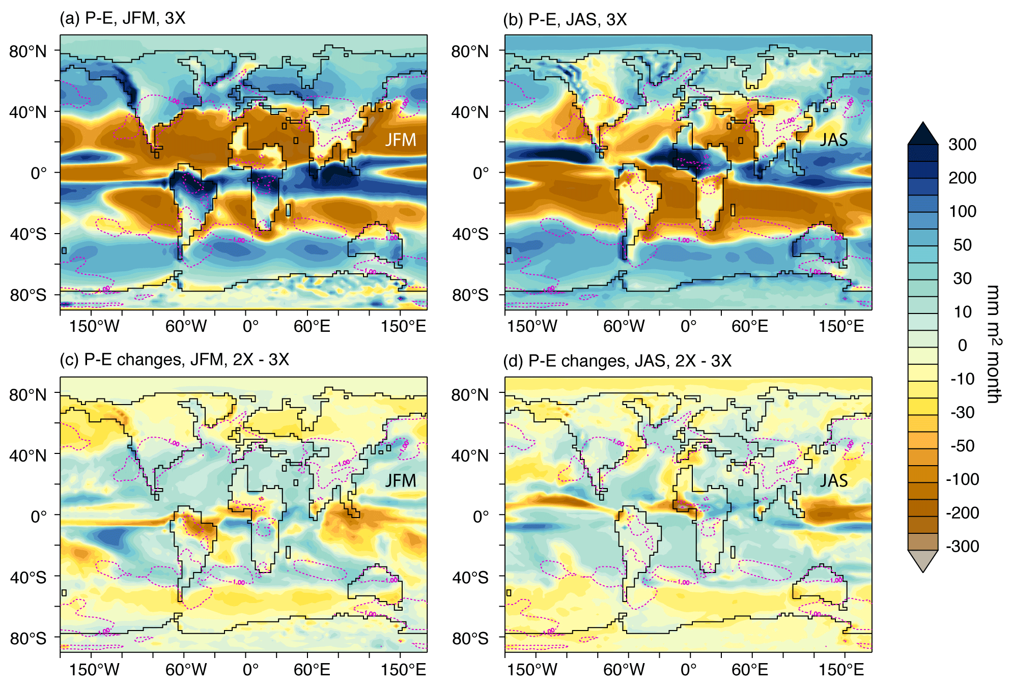
Figure 5Net precipitation (precipitation − evaporation) in JAS and JFM for the late Eocene simulation 3X (a, b). Changes associated with pCO2 drop from 3X to 2X (differences shown are 2X−3X) for net precipitation (c, d). Magenta dashed lines contour areas with decreased seasonality (ΔMATR ∘C) in 2X−3X simulations (blue zones in Fig. 4b).
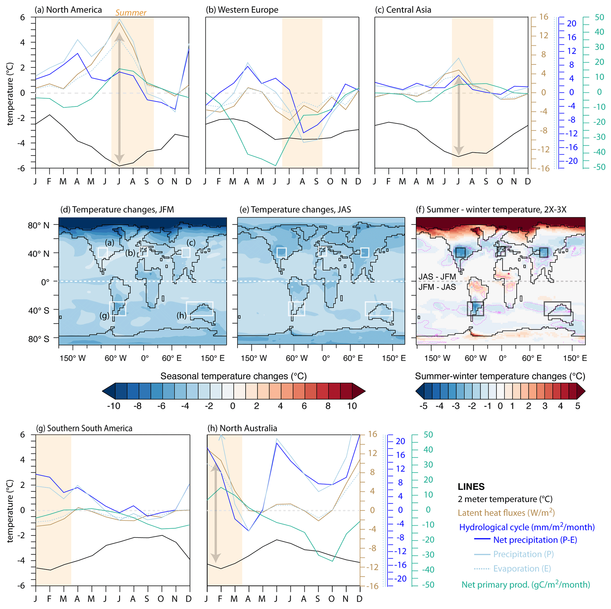
Figure 6Annual variability of multiple climate parameters within the different areas of decreasing seasonality between 3X and 2X (a–c, g, h): atmospheric temperature (black), latent heat fluxes (soil to atmosphere; brown), hydrological cycle (including precipitation, evaporation and net precipitation; different shades of blue) and net primary productivity (green). Temperature changes and summer−winter temperature changes (d–f). Rectangles outline the land areas analyzed in (a)–(c), (g) and (h) (ocean zones are not taken into account in the calculation of the plots). Gray arrows show where decreasing summer temperatures match increased latent heat fluxes.
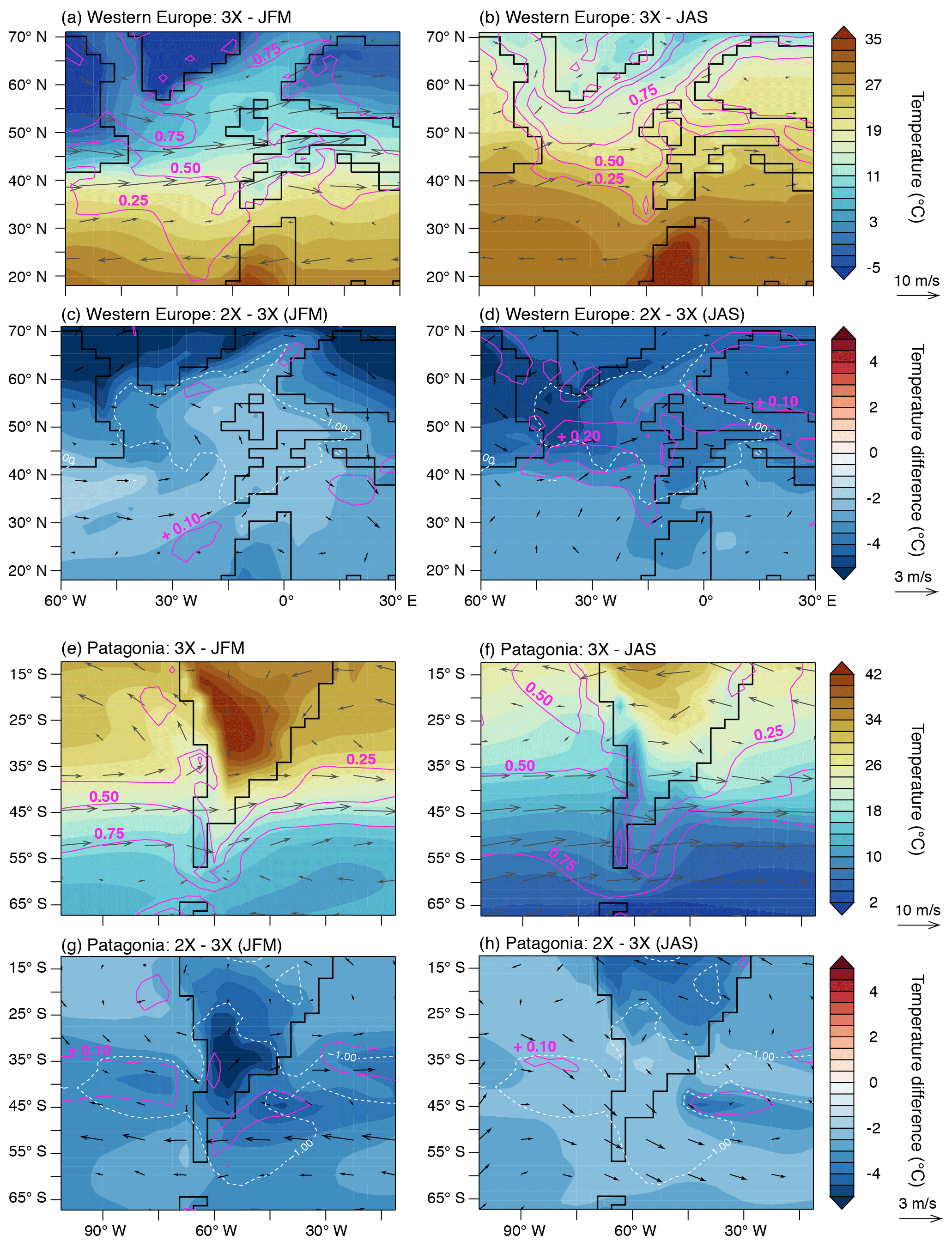
Figure 7Two-meter atmospheric temperature across western Europe and Patagonia. Shadings correspond to temperatures (a, b, e, f) and temperature differences (c, d, g, h). Similarly, magenta lines contour low-level fraction (a, b, e, f) and low-level cloud fraction changes (c, d, g, h; always expressed in %) and arrows, 850 hPa winds (a, b, e, f) and 850 hPa wind changes (c, d, g, h; always in m s−1). White dashed lines contour areas with decreased seasonality (ΔMATR ∘C) in 2X−3X simulations (blue zones in Fig. 4b).
3.2 Modeled response to Antarctic ice sheet and sea-level drop
3.2.1 Antarctic ice sheet only
AIS formation is responsible for a supplementary 0.9 and 0.3 ∘C cooling of the air temperature and the surface ocean, respectively (Table 1). Its direct effect on 2 m mean annual temperatures varies regionally and is more striking over Antarctica with up to −35 ∘C cooling and over the Southern Ocean and Australia (Figs. 2c, g, k and S3c and d). In contrast with Arctic sea ice which increases seasonality at the highest northern latitudes, the AIS decreases southern latitude temperature seasonality (Figs. 4c and S3c and d). Indeed, simulations with the AIS have a yearlong white Antarctica with high and stable albedo, which reduces seasonal temperature variability (Fig. 3g–l).
3.2.2 Sea-level drop
Sea-level decrease alone is responsible for a 1.0 ∘C cooling of global MAT (0.7 ∘C for surface oceans) and results in considerable regional temperature changes in areas with important land–sea distribution changes (Table 1, Figs. 4d and f and S3e and f). The marine regions that become exposed after sea-level drop show the strongest increase in MATR, as they experience both winter cooling and summer warming, due to the lower thermal inertia of land compared to ocean. This seasonality strengthening in newly exposed areas occurs independently of their latitude, therefore disrupting the otherwise zonal distribution of seasonal temperature changes generated by pCO2 drop and AIS formation (Figs. 4f and S3f). The effect on seasonality of these disappearing seas expands beyond areas adjoining the emerging landmasses due to the resulting regional perturbation in temperature. Northern Africa, western Asia and Russia are the most impacted areas, due to the retreat of the proto-Paratethys sea and the emergence of the Arabian Peninsula (Fig. 1). More moderate seasonality changes are also visible as a result of sea retreats of smaller extent, such as the emergence of the Florida platform and the modification of the East Asian coastlines (Figs. 4d and S3e and f).
3.3 Model–data comparison
3.3.1 pCO2 lowering
The ΔMATR described by the pCO2 drop experiments (from 3X or 4X to 2X) show no good agreement either with middle to late Eocene or with late Eocene to early Oligocene data estimates (Figs. 4a and b and 8b). The simulations predict no change, or a MATR decrease, in areas where the Lutetian–Priabonian data points (n=6, triangles, Fig. 4a) describe increased seasonality (Fig. 4a and b). Priabonian–Rupelian ΔMATR modeled through 4X to 2X and 3X to 2X pCO2 drops is, on average, lower than data estimates at similar localities, with a mean offset of −3.5 and −2.8 ∘C, respectively (Fig. 8b; Table 2). The use of the simulation 4X instead of 3X for the late Eocene stage has a marginal effect on the percentage of agreement for the sign of the ΔMATR, although a slightly higher value is observed for 3X–2X (Table 2, line “%”, Figs. 8b and S9). In addition, the pCO2 drop alone leads to zonal ΔMATRs which do not transcribe the spatial heterogeneity visible in data. This misfit is visible through high RMSE scores and the absence of significant correlation between modeled ΔMATR resulting from the pCO2 drop (simulations 2X–4X and 2X–3X) and ΔMATR described by proxy data (Table 2). Two data–model agreement patterns are nevertheless to be noted: (1) regardless of their values (which are higher in data than in our simulations), the northernmost data points are inside or surround the high-latitude seasonality strengthening zone we modeled (Fig. 4, data points 1, 2 and 3 in Fig. 8a); (2) none of the Southern Hemisphere data localities showing no seasonality change are located within MATR increase zones (Fig. 4b).
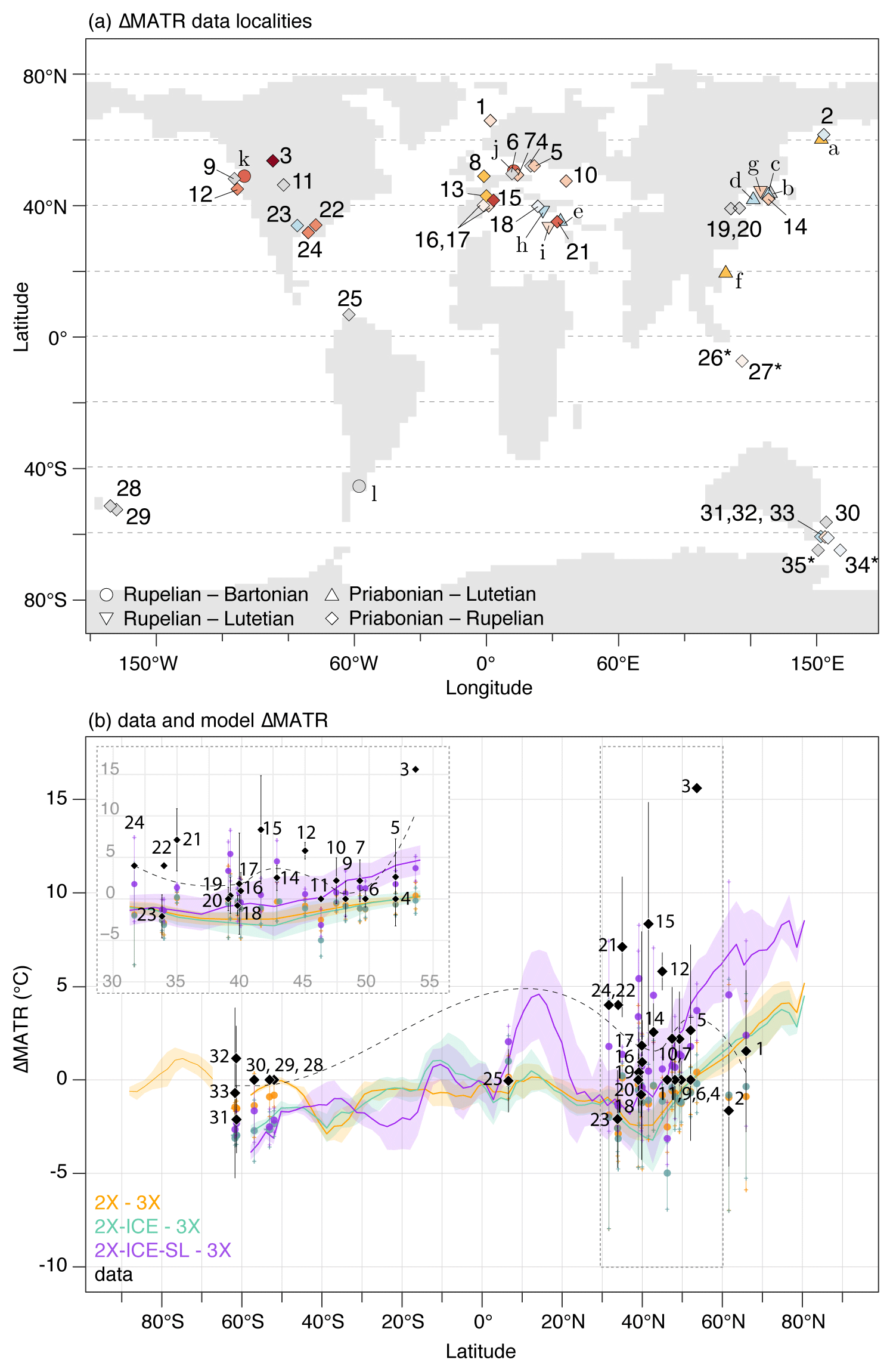
Figure 8Data–model comparison of ΔMATR from the Priabonian to the Rupelian. (a) Map of all data ΔMATR estimates compiled in this study (symbols refer to the time period compared for the calculation of the MATR shift; see Table S1 in the Supplement for associated references). The points marked with an asterisk have an uncertain origin (marine sediments) and have not been taken into account in the statistical analyses although they are shown here. The points marked with an asterisk have an uncertain origin (marine sediments) and have not been taken into account in the statistical analyses although they are shown here. (b) Comparison of data estimates of Priabonian–Rupelian ΔMATR (black diamonds) to modeled ΔMATR at the same localities (colored circles, calculated over a area) from different pairs of simulations with 3X. Error bars are minimum and maximum data estimates of ΔMATR. The dashed black line is the LOESS curve associated with data ΔMATR estimates. Bold colored lines indicate the continental latitudinal gradient of ΔMATR on land (i.e., all longitudes averaged per degree of latitude); color-shaded intervals are the standard deviation around the average. A subfigure similar to (b) but using the simulation 4X as a Priabonian stage is available in the Supplement, Fig. S9.
Table 2Priabonian–Rupelian data–model comparison. Negative mean ΔMATR values reflect a tendency of the model to underestimate ΔMATRs. The line “%” gives the percentage of sites where the direction of ΔMATR is adequately modeled (e.g., the model described a MATR reinforcement in the zone where data indicate MATR increase). Modeled ΔMATR estimates were regarded as positive when >0.5, negative when <0.5, or null when in the range of [−0.5; 0.5]. ρ indicates the strength of the correlation estimated with the Spearman rank test, with associated p values (p). Note that with all p values being >0.05, none of the correlations are significant.

3.3.2 Antarctic ice sheet and sea level
The formation of the AIS alone does not result in a better agreement between modeled and Priabonian–Rupelian ΔMATR estimates. It is even slightly reduced (Table 2). The reinforcement of the MATR lowering zone at high southern latitudes increases the data–model misfit because of data points indicating null ΔMATR in this zone (Figs. 4c and 8b). There is still no significant correlation between ΔMATR from the model and differences documented by proxy data (Table 2).
Geographic changes associated with sea-level drop result in a better agreement with data ΔMATR (Figs. 4d and 8b). The largest continental fraction changes affect the MATR on a broad geographic scale and allow for a better agreement, even with several data points standing away from the regions directly impacted by the sea-level drop, as for example data estimates located on the Pacific Coast (Fig. 4d). Similarly, coastline changes along the eastern part of Africa and western Asia cause an increase in seasonality in Anatolia and central/western Europe, improving the fit between model and data. These changes in temperature seasonality result in a reduction of 2 to 2.5 months in the duration of the plant growing season (as reconstructed with the formula of Grein et al., 2013; Table S1 in the Supplement). Smaller changes in coastlines such as in Florida, the Kamchatka Peninsula or along the East Asian coast increase seasonality at a regional scale and improve the data–model fit (data points 14, 22 and 24). This better fit is transcribed through the RMSE analysis results, the lowest values being obtained when the simulation 2X-ICE-SL is used to simulate the Rupelian stage (Table 2). However, there is no significant correlation between model and proxy-data Priabonian–Rupelian ΔMATR, independently of the late Eocene simulation (4X or 3X) used as initial stage (for both, Spearman rank test: ρ=0.29, p value =0.12, Table 2). This persistent mismatch may be triggered by biases from the model or the data and from the methodology used to calculate these ΔMATR, which are further detailed in the Discussion. ΔMATR is still slightly underestimated by the model (Fig. 8b; Table 2). The pair of simulations that best describe the Priabonian–Rupelian transition, according to currently available data is 2X-ICE-SL–3X as it presents (1) the lowest average model–data ΔMATR mismatch (−1.20 ∘C) and (2) the best agreement in ΔMATR direction (45 % of the data, Table 2).
4.1 Implication for mechanisms of late Eocene to early Oligocene seasonality changes
4.1.1 Model climate sensitivity and climate response to EOT forcing
ΔMATR across the EOT are better predicted when considering the changes occurring between the lower pCO2 simulation 3X for the late Eocene stage and the most realistic simulation 2X-ICE-SL for the early Oligocene stage. In addition, with a mean SST cooling of 2.7 ∘C between 3X and 2X simulations (Table 1), surface temperature changes are also in agreement with the mean changes described in marine proxies across the EOT (i.e., difference of 2.9 ∘C between 38–34.2 and 33.7–30 Ma, Hutchinson et al., 2021). This best fit with a limited drop in pCO2 reflects the high climate sensitivity of our model (i.e., the average temperature change per doubling of the pCO2 at model equilibrium; PALAEOSENS, 2012). This high sensitivity is also highlighted in our experiments of pCO2 halving from 1120 to 560 ppm (2X–4X), which result in a dramatic mean annual global cooling (5.8 ∘C for global MAT, 5 ∘C for SST, Table 1). Such a temperature difference is high compared to previous modeling studies which describe a 3 to 4 ∘C surface atmospheric temperature difference under a similar pCO2 decrease and the 2.9 ∘C cooling found in marine proxies across the EOT (Hutchinson et al., 2021). The pCO2 of 4X and 2X is commonly used in simulations to represent the transition to an icehouse world (e.g., Baatsen et al., 2020; Goldner et al., 2014; Kennedy-Asser et al., 2019). Although 4X is likely to represent the upper end of pCO2 possible values for the late Eocene (the average values are rather close to 800 ppm from the Lutetian to the Priabonian; Foster et al., 2017), the use of this value is justified to better reconstruct high-latitude temperatures (Huber and Caballero, 2011). A good agreement between warm conditions and Bartonian SST data has also been recently shown by other experiments using the model IPSL-CM5A2 with middle/late Eocene boundary conditions (Tardif et al., 2020; Toumoulin et al., 2020). We thus argue that although the use of the 4X simulation is appropriate to study possible variations in pCO2 during the Eocene, the use of the 3X simulation is better to study the changes between the Priabonian and the Rupelian.
4.1.2 Temperature seasonality changes through the late Eocene
The evolution of the different climate features likely involved in ΔMATR is consistent with several findings from previous studies. First, earlier modeling experiments have described albedo and sea-ice increase resulting in polar amplification of the cooling (e.g., Baatsen et al., 2020; Kennedy-Asser et al., 2019) and a reinforcement of temperature seasonality (Eldrett et al., 2009). The resulting strengthening and expansion of the northern high-latitude MATR increase zone with pCO2 lowering is a good explanation for the dramatic seasonality increase at high latitudes suggested by some studies (Eldrett et al., 2009; Wolfe, 1992; Zanazzi et al., 2015). In addition, changes in the magnitude and distribution of net precipitation (i.e., precipitation – evaporation) resulting from the decrease in pCO2 agree with previous theoretical and modeling work suggesting an intensified hydrological cycle under higher pCO2 (e.g., Carmichael et al., 2016; Hutchinson et al., 2018). This phenomenon results from a greater capacity of the air to retain moisture and more intense atmospheric convection phenomena (Allen and Ingram, 2003; Carmichael et al., 2016; Held and Soden, 2006). In parallel, although the implication of changes in the atmospheric circulation in the southern South American seasonality lowering zone appears non-obvious, the intensification and weakening of the Hadley cell extent in relation to changing pCO2 levels have been described numerous times (e.g., Lu et al., 2007; Frierson et al., 2007). Deeper analyses would be needed to understand the atmospheric dynamics in the simulations, which is beyond the scope of the study. Finally, the increase in low cloud cover is consistent with previous model studies describing a higher fraction of low-level clouds under lower pCO2 (Baatsen et al., 2020; Caballero and Huber, 2013; Zhu et al., 2019). Nevertheless, although a low-level cloud cover increase due to the pCO2 drop is consistent with increased air moisture in western Europe at the EOT (Kocsis et al., 2014), this parameter remains poorly constrained in paleoclimate archives and modeling analysis (Lunt et al., 2020; Sagoo et al., 2013).
Despite these agreements, the MATR evolution resulting from the pCO2 drop does not clearly match data estimates, whether they correspond to both Lutetian–Priabonian or to Priabonian–Rupelian changes. This suggests that the temperature seasonality inferred from proxy data can only be partly explained by a pCO2 drop. Since zonal ΔMATR patterns are simulated with a pCO2 drop of 1 PAL (either from 4X to 3X or from 3X to 2X), we hypothesize that they likely occurred before the AIS onset and that the strengthening of seasonality occurred in northern high latitudes in the first place. However, most Lutetian–Priabonian data are not located in the high latitudes, which prevents unambiguous testing of this hypothesis (Fig. 4a and b and Table S1 in the Supplement). Similarly, the presence of areas with decreased seasonality due to changes in the hydrological cycle (i.e., the USA, Central Asia, north Australia) cannot be confirmed because of a lack of data in these areas: although some of the data associated with a decrease in the MATR share the same latitudinal bands, none of them are directly located within a zone of MATR decrease. New additional seasonal temperature records in these areas would be interesting to better trace such eventual early trends. The general low fit of data and model values for middle to late Eocene changes is, to some extent, predictable since the ice-free 2X simulation does not represent the late Eocene (see “Material and methods” section) and was designed as a sensitivity test. Indeed, small-scale glaciations (25 %–35 % modern AIS) may have existed during the late Eocene, before the EOT, associated with a moderate sea-level decrease (Carter et al., 2017; Miller et al., 2020; Scher et al., 2014). Interestingly, the combination of the three forcing mechanisms leads to a better agreement of the modeled ΔMATR with some of the few middle to late Eocene data, especially in coastal areas of Kamchatka, and southern China (triangles, Fig. 4). Although the 70 m sea-level decrease prescribed in the 2X-ICE-SL simulation is unrealistic for the late Eocene, the better data–model agreement when both AIS and sea-level decrease are considered suggests that small ice-sheet development before the EOT may have played a significant role in driving the middle to late Eocene ΔMATR. Additional sensitivity experiments, with a smaller AIS and an intermediated sea-level drop, may allow further quantification of the sensitivity of coastal localities to sea-level variations occurring before the EOT.
4.1.3 Temperature seasonality changes through the EOT
The use of two simulations to set up the effect of the AIS onset (with or without a drop in sea level) is interesting to unravel the direct and indirect mechanisms affecting temperatures. Temperature changes resulting from the presence of the AIS alone (i.e., not taking into account sea level) are consistent with previous model studies that simulate its highly regional effect on atmospheric temperature (see the Supplement of Hutchinson et al., 2021), although the changes in our simulations spread more widely over the Southern Ocean and Australia. The decreasing seasonality zones modeled at high latitudes and midlatitudes of the Southern Hemisphere are mostly associated with an absence of seasonality change in the data, which often display stable vegetation and biomes from the late Eocene to the Rupelian (Hutchinson et al., 2021; Kohn et al., 2015; Nott and Owen, 1992; Pocknall, 1989; Pound and Salzmann, 2017). This apparent mismatch calls into question the capability of paleobotanical proxies to record a temperature seasonality decrease in environments already characterized by low seasonality. Indeed, the decrease in the temperature seasonality is associated with a more pronounced drop in summer temperatures, which is a less limiting factor for flora distribution and thus less constrained in the fossil record than winter temperatures (Huber and Caballero, 2011).
The evolution of temperature seasonality from the Priabonian to the Rupelian is better represented when the sea-level drop associated with the AIS is taken into account (Table 2, Figs. 4 and 8). This consequence of the Antarctic glaciation has global repercussions and explains part of the heterogeneity documented in the data, as previously suggested (Pound and Salzmann, 2017). Our results are very dependent on the paleogeography used in the simulations and of the proxy location used in our data–model comparison. Because our Rupelian simulations use a late Eocene paleogeography with a global sea-level decrease, we overlook some paleogeographic changes that occurred between both periods, which may affect our seasonality reconstruction. The gradual northward migration of Australia is not considered; the Neotethys is gradually closed during the early Oligocene, but a deep-sea passage to the north of the Arabian Plate remains present in our paleogeography (Barrier et al., 2018). Another source of error may come from fragmented continental areas such as those seen in Europe at that time. In these zones, temperature changes recorded through the EOT are heterogeneous as paleovegetation studies suggest medium (1.8–2.1 ∘C; Moraweck et al., 2019; Teodoridis and Kvaček, 2015; Tosal et al., 2019) to strong (up to 8.3 ∘C; Tanrattana et al., 2020) MATR increase. The heterogeneity shown in data might thus result from smaller-scale paleogeographic changes through the EOT that are not well represented by the resolution used in our simulations. This variability of the data ΔMATR estimates could also be due to (1) a variable quality of MATR data related to the fragmentary nature of the fossil record and to differential recording of vegetation types as well as (2) differences in the temperature of marine/oceanic zones before regression. Depending on their extension and depth, these seas may have buffered seasonal temperature variations in the nearby regions more or less importantly, and therefore their disappearance may have affected the MATR at different magnitudes. An early Oligocene intensification of seasonality in central and eastern Europe, associated with a major phase of Antarctic ice-sheet expansion (and its effect on sea level), is consistent with fairly stable vegetation between the middle and late Eocene (Bozukov et al., 2009; Kvaček et al., 2014; Moraweck et al., 2015). This may result from the proximity with the warm Tethys, buffering the EOT cooling, as suggested by stable δ18O describing moderate temperature changes in this area (Kocsis et al., 2014).
Finally, differences between our modeling results and data may also be related to the amplitude of the sea-level drop used in our simulation compared to its variability during the Rupelian. The EOT is generally described in two steps: a first event at ∼33.9 Ma with both a decrease in temperature and sea level (∼25 m) and a second event, the Early Oligocene Glacial Maximum (EOGM), between approximately 33.65 and 33.15 Ma, starting after a large oxygen isotope incursion (often referred to as “Oi-1”), which is characterized by an additional 50 m sea-level decrease (see Hutchinson et al., 2021, for synthesis and terminology, and Miller et al., 2020). The sum of these two steps corresponds to the boundary conditions of our simulation. However, important variations in the East Antarctic Ice Sheet have been described until the early Miocene (50–60 m sea-level equivalent; Miller et al., 2020). Directly after the EOGM phase, a decrease in ice volume is visible between 33.15 and 32.8 Ma, before it increases again and remains stable between 32.8 and 29 Ma (after the Oi-1a event; Galeotti et al., 2016). Due to the combined effects of the drop in CO2 and the development of the AIS (and the amplitude of the associated drop in sea level, 70 m), the important changes in seasonality reconstructed here (2X-ICE-SL−3X) were probably not in place throughout the Rupelian but rather for shorter periods during the EOGM, or later between 32.8–29 Ma. Most continental paleoclimate studies do not provide the resolution to distinguish these steps. Among the data points compiled for this study, only four sites have enough temporal resolution to be linked to the EOGM phase represented by our 2X-ICE-SL simulation (Bozukov et al., 2009; Hren et al., 2013; Kohn et al., 2015; Tosal et al., 2019).
4.2 Perspectives on environmental and biotic crisis
The EOT is associated with major extinction events, of which the best known are the Grande Coupure in Europe and the Mongolian Remodeling in central Asia (Stehlin, 1909; Meng and McKenna, 1998; see Coxall and Pearson, 2007, for a review). Both events have been recognized as major biotic turnovers for ungulates (Blondel, 2001; Stehlin, 1909). In addition, other vertebrates were affected by the Grande Coupure (e.g., rodents, primates, amphibians and squamates), and major changes in vegetation are described, in association with the Mongolian Remodeling and regionally, in Europe (e.g., Barbolini et al., 2020; Marigó et al., 2014; Pound and Salzmann, 2017; Rage, 1986, 2013; Roček and Rage, 2003). These changes have been linked to (1) competitive interactions resulting from the dispersal of Asian taxa to Europe and (2) EOT climate deterioration and selection processes through resource and/or habitat changes (e.g., Hooker et al., 2004; Kratz and Geisler, 2010; Marigó et al., 2014; Sun et al., 2015; Zhang et al., 2012). The latter mechanism is commonly related to irreversible cooling and/or aridification at the EOT (e.g., Blondel, 2001; Sun et al., 2015; Zhang et al., 2012). Climate cooling may have significantly reduced the habitat of well-spread early Eocene tropical (and paratropical) species, which are characterized by narrow thermal ecological niches (Hren et al., 2009; Huang et al., 2020; Jaramillo et al., 2006; Wing, 1987). Although the distribution of fauna and flora is based on a complex set of parameters, we discuss here how ΔMATR provides an additional interpretative key for understanding biotic turnover at the EOT.
While North America and Asia show comparable temperature changes, our simulations highlight significant differences in the evolution of their MATR, which decreases and either increases/decreases at a regional scale, respectively. Vegetation changes and the Mongolian Remodeling are contemporaneous to AIS growth between 32.8–29 Ma and can be compared with our 2X-ICE-SL simulation (Galeotti et al., 2016; Kraatz and Geisler, 2010; Sun et al., 2015). The MATR strengthening modeled in central Asia shows that cooling was particularly strong during winter. In addition to the aridification, this more pronounced winter cooling may have contributed to the intensity of extinctions in this area (Barbolini et al., 2020; Dupont-Nivet et al., 2007). This seasonality strengthening is strongly driven by the proto-Paratethys retreat, which contrasts with a previous geochemistry study suggesting a weak contribution of this sea to local climate conditions (Bougeois et al., 2018). Conversely, the zone of decreased MATR reconstructed in North America may provide an explanation for the low impact of the EOT on fauna and vegetation in this area (Coxall and Pearson, 2007; Prothero and Heaton, 1996; Stucky, 1992). Despite a similar decrease in the mean annual temperature, most of the temperature drop is in summer and is not associated with the onset of cold winters (Fig. S4). We hypothesize that these patterns enabled a greater persistence of existing warm-temperate to paratropical vegetation and associated biota (Pound and Salzmann, 2017). The study of Tardif et al. (2021) using the same model and similar simulations (4X and 2X-ICE) with a dynamic vegetation module shows moderate biome changes across the EOT in this North America decreased seasonality zone. Reduced stress on biodiversity in areas with limited or reduced MATR changes is also consistent with moderate vegetation changes across the EOT in areas with decreasing seasonality in the Southern Hemisphere (see discussion in Sect. 4.1.3).
Europe stands in an intermediate position between North America and Asia with generally weaker changes in MATR (Fig. 4d); eastern Europe exhibits a slight increase in MATR, while MATR decreases in the west. Although comparable ΔMATR values could have different impacts depending on initial MATR, the types of ecosystems and their resilience, the strong consequences of moderate seasonality increase on growing season length support the hypothesis that seasonality changes may also have contributed to shaping the biodiversity evolution in central Europe. The late development of increased seasonality zones in this area, linked to the major phase of sea-level drop, could explain the persistence of fairly stable vegetation during the Eocene (Kvaček et al., 2014; Hutchinson et al., 2021). Yet, given the fragmented nature of Europe at this time, increases in seasonality prior to the EOT would also be possible as a result of smaller, but locally significant, sea-level variations. These differences in the evolution of the MATR between North America, Europe and Asia are consistent with several studies suggesting different causes for EOT extinctions (Blondel, 2001; Hooker et al., 2004; Meng and McKenna 1998; Sun et al., 2015). Finally, little is known about the EOT in Africa (notably because of a few Oligocene sites), but the data available suggest moderate changes in northern African flora and fauna (Hutchinson et al., 2021; Jacobs et al., 2010; Pound and Salzmann, 2017; Rasmussen et al., 1992). The significant increase in seasonality in North Africa seen in our simulations (which results from the emergence of part of the continent) differs from the one observed in other areas, since it is linked to an increase in summer temperatures (barely no change in winter). Unchanged winter temperatures and the shift of marine to terrestrial environments might complicate the recording of this temperature seasonality strengthening. Recording low-latitude changes in seasonality strengthening may however be possible as shown by a recent study combining multiple lines of evidences (including plant and primate macrofossils), which suggest a potential shift from tropical to more open deciduous vegetation through the EOT, reflecting increased seasonality in precipitation and/or temperature seasonality during the early Oligocene at low latitudes of South America (Peru, S, Antoine et al., 2021). More studies would probably enable a better understanding of the evolution of the seasonality in this low-latitude area.
This study investigates the changes in temperature seasonality during the middle to late Eocene and across the EOT. MATR changes modeled with the combined effects of pCO2 drop, AIS formation and sea-level lowering are qualitatively consistent with the proxy-data reconstruction of the late Eocene to early Oligocene. The decrease in pCO2 leads to a marked strengthening of seasonality in the northern high latitudes, which may have started earlier than the EOT, during the late Eocene. The formation of the AIS and the resulting sea-level drop lead to both an intensification and an extension of increasing seasonality areas. The best agreement between data and modeled MATR evolution throughout the EOT is reached when all three parameters are combined. Accounting for sea-level changes associated with the Antarctic glaciation appears to be the most important parameter to explain the heterogeneity of ΔMATR across the EOT. A seasonality increase is also visible in middle to late Eocene localities, which may reflect earlier sea-level changes associated with the incipient precursors of the Antarctic ice sheet. A discrepancy between data and model is present for quantitative MATR change estimates across the EOT, with less marked seasonality changes in the model. This is mainly due to areas where a decrease in seasonality is predicted by the model while the vegetation proxies show stable vegetation. We hypothesize that this discrepancy can be explained by a low capacity of vegetation to record decreases in summer temperatures compared to winter temperatures.
Reconstructing changes in MATR brings additional constraints on the abiotic environmental factors at play on land between the middle Eocene and the early Oligocene. The different mechanisms described here likely explain the heterogeneity in seasonality changes found in data across the greenhouse–icehouse transition and provide insights into the diversity of continental paleoenvironments. The map of ΔMATR reconstructed here give new elements to help understand major extinction events of the EOT. This study primarily focused on the evolution of temperature seasonality that has the clearest evolution. The variability of other seasonality parameters, including rainfall seasonality, will be worth investigating in future studies to obtain a finer picture of the evolution of terrestrial climates and biodiversity through the EOT. In addition, further work using higher-resolution Rupelian paleogeography and regional models would be of great interest to better reconstruct temperature seasonality changes, especially in highly fragmented land areas such as Europe during the Eocene.
LMDZ, XIOS, NEMO and ORCHIDEE are released under the terms of the CeCILL license. OASISMCT is released under the terms of the Lesser GNU General Public License (LGPL). The IPSL-CM5A2 code is publicly available through svn, with the following command lines: svn co http://forge.ipsl.jussieu.fr/igcmg/svn/modipsl/branches/publications/IPSLCM5A2.1_11192019 (IPSL Climate Modelling Centre, 2022a), modipsl cd modipsl/util;./model IPSLCM5A2.1
The mod.def file provides information regarding the different revisions used, namely
-
NEMOGCMbranchnemo_v3_6_STABLErevision666-XIOS2branchs/xios-2.5revision1763
-
IOIPSL/srcsvntags/v2_2_2
-
LMDZ5branches/IPSLCM5A2.1rev3591
-
branches/publications/ORCHIDEE_IPSLCM5A2.1.r5307rev
6336–OASIS3-MCT2.0_branch(rev4775IPSLserver).
The login/password combination requested for the first use to download the ORCHIDEE component is anonymous/anonymous. We recommend referring to the project website http://forge.ipsl.jussieu.fr/igcmg_doc/wiki/Doc/Config/IPSLCM5A2 (IPSL Climate Modelling Centre, 2022b) for a proper installation and compilation of the environment.
The key climatological outputs of the simulations are stored in the PANGAEA database: https://doi.pangaea.de/10.1594/PANGAEA.930422 (Toumoulin et al., 2021).
The supplement related to this article is available online at: https://doi.org/10.5194/cp-18-341-2022-supplement.
YD, AT and JBL conducted the modeling experiments. AT compiled proxy data, analyzed the model results, generated figures and tables, and drafted the paper. AT, YD, DT and JBL discussed the paleoclimate results. LK contributed to the paleobotanical context and AL and GDN to the paleogeographic and geological context. All authors have provided critical feedback and contributed to the final paper.
The contact author has declared that neither they nor their co-authors have any competing interests.
Publisher’s note: Copernicus Publications remains neutral with regard to jurisdictional claims in published maps and institutional affiliations.
We thank the CEA/CCRT for providing access to the HPC resources of TGCC under the allocation 2018-A0030102212, and 2019-A0050102212 made by GENCI. Agathe Toumoulin and Guillaume Dupont-Nivet acknowledge the support of the ERC MAGIC under grant 649081. Yannick Donnadieu and Delphine Tardif acknowledge support from ANR AMOR (grant no. ANR-16-CE31-0020). The authors acknowledge Cheng-Sen Li for sharing a translation of the reference Budantsev (1997). We acknowledge the use of Ferret (https://ferret.pmel.noaa.gov/Ferret/, last access: 10 November 2021) and RStudio software (https://www.rstudio.com/, last access: 10 November 2021) for analysis and figures in this paper. We sincerely thank Alberto Reyes for his editorial handling and two anonymous reviewers for their interesting comments that improved the quality of this article.
This research has been supported by ERC MAGIC (grant no. 649081) and ANR AMOR (grant no. ANR-16-CE31-0020). The article processing charges for this open-access publication were covered by ANR AMOR (ANR-16-CE31-0020).
This paper was edited by Alberto Reyes and reviewed by two anonymous referees.
Allen, M. R. and Ingram, W. J.: Constraints on future changes in climate and the hydrologic cycle, Nature, 419, 228–232, https://doi.org/10.1038/nature01092, 2002.
Antoine, P.-O., Yans, J., Castillo, A. A., Stutz, N., Abello, M. A., Adnet, S., Custódio, M. A., Benites-Palomino, A., Billet, G., Boivin, M., Herrera, F., Jaramillo, C., Mártinez, C., Moreno, F., Navarrete, R. E., Negri, F. R., Parra, F., Pujos, F., Rage, J.-C., Ribeiro, A. M., Robinet, C., Roddaz, M., Tejada-Lara, J. V., Varas-Malca, R., Ventura Santos, R., Salas-Gismondi, R., and Marivaux, L.: Biotic community and landscape changes around the Eocene–Oligocene transition at Shapaja, Peruvian Amazonia: Regional or global drivers?, Global Planet. Change, 202, 103512, https://doi.org/10.1016/j.gloplacha.2021.103512, 2021.
Aumont, O., Ethé, C., Tagliabue, A., Bopp, L., and Gehlen, M.: PISCES-v2: an ocean biogeochemical model for carbon and ecosystem studies, Geosci. Model Dev., 8, 2465–2513, https://doi.org/10.5194/gmd-8-2465-2015, 2015.
Baatsen, M., von der Heydt, A. S., Huber, M., Kliphuis, M. A., Bijl, P. K., Sluijs, A., and Dijkstra, H. A.: The middle to late Eocene greenhouse climate modelled using the CESM 1.0.5, Clim. Past, 16, 2573–2597, https://doi.org/10.5194/cp-16-2573-2020, 2020.
Barbolini, N., Woutersen, A., Dupont-Nivet, G., Silvestro, D., Tardif, D., Coster, P. M. C., Meijer, N., Chang, C., Zhang, H.-X., Licht, A., Rydin, C., Koutsodendris, A., Han, F., Rohrmann, A., Liu, X.-J., Zhang, Y., Donnadieu, Y., Fluteau, F., Ladant, J.-B., Hir, G. L., and Hoorn, C.: Cenozoic evolution of the steppe-desert biome in Central Asia, Sci. Adv., 6, eabb8227, https://doi.org/10.1126/sciadv.abb8227, 2020.
Barrier, E., Vrielynck, B., Brouillet, J.-F., and Brunet, M.-F.: Paleotectonic Reconstruction of the Central Tethyan Realm. Tectonono-Sedimentary-Palinspastic maps from Late Permian to Pliocene, CCGM/CGMW, Paris, available at: http://www.ccgm.org (last access: 18 February 2022), 2018.
Bishop, P. and Bamber, R. K.: Silicified wood of Early Miocene Nothofagus, Acacia and Myrtaceae (aff. Eucalyptus B) from the upper Lachlan valley, New South Wales, Alcheringa, 9, 221–228, https://doi.org/10.1080/03115518508618969, 1985.
Blondel, C.: The Eocene – Oligocene ungulates from Western Europe and their environment, Palaeogeogr. Palaeocl., 168, 125–139, https://doi.org/10.1016/S0031-0182(00)00252-2, 2001.
Bougeois, L., Dupont-Nivet, G., de Rafélis, M., Tindall, J. C., Proust, J.-N., Reichart, G.-J., de Nooijer, L. J., Guo, Z., and Ormukov, C.: Asian monsoons and aridification response to Paleogene sea retreat and Neogene westerly shielding indicated by seasonality in Paratethys oysters, Earth Planet Sci. Lett., 485, 99–110, https://doi.org/10.1016/j.epsl.2017.12.036, 2018.
Bozukov, V., Utescher, T., and Ivanov, D.: Late Eocene to early Miocene climate and vegetation of Bulgaria, Rev. Palaeobot. Palyno., 153, 360–374, https://doi.org/10.1016/j.revpalbo.2008.10.005, 2009.
Budantsev, L. Y.: Late Eocene flora of western Kamchatka, Proceedings of Komarov Botanical Institute, Russian Academy of Sciences, 19, 1–115, 1997.
Caballero, R. and Huber, M.: State-dependent climate sensitivity in past warm climates and its implications for future climate projections, P. Natl. Acad. Sci., 110, 14162–14167, https://doi.org/10.1073/pnas.1303365110, 2013.
Carmichael, M. J., Lunt, D. J., Huber, M., Heinemann, M., Kiehl, J., LeGrande, A., Loptson, C. A., Roberts, C. D., Sagoo, N., Shields, C., Valdes, P. J., Winguth, A., Winguth, C., and Pancost, R. D.: A model–model and data–model comparison for the early Eocene hydrological cycle, Clim. Past, 12, 455–481, https://doi.org/10.5194/cp-12-455-2016, 2016.
Carter, A., Riley, T. R., Hillenbrand, C.-D., and Rittner, M.: Widespread Antarctic glaciation during the Late Eocene, Earth Planet. Sci. Lett., 458, 49–57, https://doi.org/10.1016/j.epsl.2016.10.045, 2017.
Colwyn, D. A. and Hren, M. T.: An abrupt decrease in Southern Hemisphere terrestrial temperature during the Eocene–Oligocene transition, Earth Planet. Sci. Lett., 512, 227–235, https://doi.org/10.1016/j.epsl.2019.01.052, 2019.
Coxall, H. K. and Pearson, P. N.: The Eocene–Oligocene Transition, in: Deep-Time Perspectives on Climate Change: Marrying the Signal from Computer Models and Biological Proxies, edited by: Williams, M., Haywood, A. M., Gregory, F. J., and Schmidt, D. N., The Geological Society of London on behalf of The Micropalaeontological Society, 351–387, https://doi.org/10.1144/TMS002.16, 2007.
Coxall, H. K., Wilson, P. A., Pälike, H., Lear, C. H., and Backman, J.: Rapid stepwise onset of Antarctic glaciation and deeper calcite compensation in the Pacific Ocean, Nature, 433, 53–57, https://doi.org/10.1038/nature03135, 2005.
Dufresne, J.-L., Foujols, M.-A., Denvil, S., Caubel, A., Marti, O., Aumont, O., Balkanski, Y., Bekki, S., Bellenger, H., Benshila, R., Bony, S., Bopp, L., Braconnot, P., Brockmann, P., Cadule, P., Cheruy, F., Codron, F., Cozic, A., Cugnet, D., de Noblet, N., Duvel, J.-P., Ethé, C., Fairhead, L., Fichefet, T., Flavoni, S., Friedlingstein, P., Grandpeix, J.-Y., Guez, L., Guilyardi, E., Hauglustaine, D., Hourdin, F., Idelkadi, A., Ghattas, J., Joussaume, S., Kageyama, M., Krinner, G., Labetoulle, S., Lahellec, A., Lefebvre, M.-P., Lefevre, F., Levy, C., Li, Z. X., Lloyd, J., Lott, F., Madec, G., Mancip, M., Marchand, M., Masson, S., Meurdesoif, Y., Mignot, J., Musat, I., Parouty, S., Polcher, J., Rio, C., Schulz, M., Swingedouw, D., Szopa, S., Talandier, C., Terray, P., Viovy, N., and Vuichard, N.: Climate change projections using the IPSL-CM5 Earth System Model: from CMIP3 to CMIP5, Clim. Dynam., 40, 2123–2165, https://doi.org/10.1007/s00382-012-1636-1, 2013.
Dupont-Nivet, G., Krijgsman, W., Langereis, C. G., Abels, H. A., Dai, S., and Fang, X.: Tibetan plateau aridification linked to global cooling at the Eocene–Oligocene transition, 445, Nature, 635–638, https://doi.org/10.1038/nature05516, 2007.
Eldrett, J. S., Greenwood, D. R., Harding, I. C., and Huber, M.: Increased seasonality through the Ecocene to Oligocene transition in northern high latitudes, Nature, 459, 969, https://doi.org/10.1038/nature08069, 2009.
Fichefet, T. and Maqueda, M. A. M.: Sensitivity of a global sea ice model to the treatment of ice thermodynamics and dynamics, J. Geophys. Res.-Oceans, 102, 12609–12646, https://doi.org/10.1029/97JC00480, 1997.
Foster, C. S. P., Sauquet, H., van der Merwe, M., McPherson, H., Rossetto, M., and Ho, S. Y. W.: Evaluating the Impact of Genomic Data and Priors on Bayesian Estimates of the Angiosperm Evolutionary Timescale, Syst. Biol., 66, 338–351, https://doi.org/10.1093/sysbio/syw086, 2017.
Galeotti, S., DeConto, R., Naish, T., Stocchi, P., Florindo, F., Pagani, M., Barrett, P., Bohaty, S. M., Lanci, L., Pollard, D., Sandroni, S., Talarico, F. M., and Zachos, J. C.: Antarctic Ice Sheet variability across the Eocene-Oligocene boundary climate transition, Science, 352, 76–80, https://doi.org/10.1126/science.aab0669, 2016.
Goldner, A., Huber, M., and Caballero, R.: Does Antarctic glaciation cool the world?, Clim. Past, 9, 173–189, https://doi.org/10.5194/cp-9-173-2013, 2013.
Goldner, A., Herold, N., and Huber, M.: Antarctic glaciation caused ocean circulation changes at the Eocene–Oligocene transition, Nature, 511, 574–577, https://doi.org/10.1038/nature13597, 2014.
Gough, D. O.: Solar interior structure and luminosity variations, Sol. Phys., 74, 21–34, https://doi.org/10.1007/BF00151270, 1981.
Grein, M., Oehm, C., Konrad, W., Utescher, T., Kunzmann, L., and Roth-Nebelsick, A.: Atmospheric CO2 from the late Oligocene to early Miocene based on photosynthesis data and fossil leaf characteristics, Palaeogeogr. Palaeocl., 374, 41–51, https://doi.org/10.1016/j.palaeo.2012.12.025, 2013.
Grimes, S. T., Hooker, J. J., Collinson, M. E., and Mattey, D. P.: Summer temperatures of late Eocene to early Oligocene freshwaters, Geology, 33, 189–192, https://doi.org/10.1130/G21019.1, 2005.
Grimm, G. W. and Potts, A. J.: Fallacies and fantasies: the theoretical underpinnings of the Coexistence Approach for palaeoclimate reconstruction, Clim. Past, 12, 611–622, https://doi.org/10.5194/cp-12-611-2016, 2016.
Held, I. M. and Soden, B. J.: Robust Responses of the Hydrological Cycle to Global Warming, J. Climate, 19, 5686–5699, https://doi.org/10.1175/JCLI3990.1, 2006.
Hooker, J. J., Collinson, M. E., and Sille, N. P.: Eocene–Oligocene mammalian faunal turnover in the Hampshire Basin, UK: calibration to the global time scale and the major cooling event, J. Geol. Soc., 161, 161–172, https://doi.org/10.1144/0016-764903-091, 2004.
Hourdin, F., Grandpeix, J.-Y., Rio, C., Bony, S., Jam, A., Cheruy, F., Rochetin, N., Fairhead, L., Idelkadi, A., Musat, I., Dufresne, J.-L., Lahellec, A., Lefebvre, M.-P., and Roehrig, R.: LMDZ5B: the atmospheric component of the IPSL climate model with revisited parameterizations for clouds and convection, Clim. Dyn., 40, 2193–2222, https://doi.org/10.1007/s00382-012-1343-y, 2013.
Huang, H., Morley, R., Licht, A., Dupont-Nivet, G., Grímsson, F., Zetter, R., Westerweel, J., Win, Z., Wa Aung, D., and Hoorn, C.: Eocene palms from central Myanmar in a South-East Asian and global perspective: evidence from the palynological record, Bot. J. Linn. Soc., 194, 177–206, https://doi.org/10.1093/botlinnean/boaa038, 2020.
Huber, M. and Caballero, R.: The early Eocene equable climate problem revisited, Clim. Past, 7, 603–633, https://doi.org/10.5194/cp-7-603-2011, 2011.
Hutchinson, D. K., de Boer, A. M., Coxall, H. K., Caballero, R., Nilsson, J., and Baatsen, M.: Climate sensitivity and meridional overturning circulation in the late Eocene using GFDL CM2.1, Clim. Past, 14, 789–810, https://doi.org/10.5194/cp-14-789-2018, 2018.
Hutchinson, D. K., Coxall, H. K., O'Regan, M., Nilsson, J., Caballero, R., and de Boer, A. M.: Arctic closure as a trigger for Atlantic overturning at the Eocene-Oligocene Transition, Nat. Commun., 10, 3797, https://doi.org/10.1038/s41467-019-11828-z, 2019.
Hutchinson, D. K., Coxall, H. K., Lunt, D. J., Steinthorsdottir, M., de Boer, A. M., Baatsen, M., von der Heydt, A., Huber, M., Kennedy-Asser, A. T., Kunzmann, L., Ladant, J.-B., Lear, C. H., Moraweck, K., Pearson, P. N., Piga, E., Pound, M. J., Salzmann, U., Scher, H. D., Sijp, W. P., Śliwińska, K. K., Wilson, P. A., and Zhang, Z.: The Eocene–Oligocene transition: a review of marine and terrestrial proxy data, models and model–data comparisons, Clim. Past, 17, 269–315, https://doi.org/10.5194/cp-17-269-2021, 2021.
IPSL Climate Modelling Centre: IPSL-CM5A-VLR branche IPSLCM5A2.1_11192019, IPSL [code], available at: http://forge.ipsl.jussieu.fr/igcmg/svn/modipsl/branches/publications/IPSLCM5A2.1_11192019, last access: 16 February 2022a.
IPSL Climate Modelling Centre: IPSL climate models documentation, IPSL [code], available at: http://forge.ipsl.jussieu.fr/igcmg_doc/wiki/Doc/Config/IPSLCM5A2, last access: 16 February 2022b.
Ivany, L. C., Patterson, W. P., and Lohmann, K. C.: Cooler winters as a possible cause of mass extinctions at the Eocene/Oligocene boundary, Nature, 407, 887–890, https://doi.org/10.1038/35038044, 2000.
Jacobs, B. F., Pan, A. D., and Scotese, C. R.: A Review of the Cenozoic Vegetation History of Africa, in: Cenozoic Mammals of Africa, University of California Press, https://doi.org/10.1525/california/9780520257214.003.0005, 2010.
Jaramillo, C., Rueda, M. J., and Mora, G.: Cenozoic Plant Diversity in the Neotropics, Science, 311, 1893–1896, https://doi.org/10.1126/science.1121380, 2006.
Joomun, S. C., Hooker, J. J., and Collinson, M. E.: Changes in dental wear of Plagiolophus minor (Mammalia: Perissodactyla) across the Eocene–Oligocene transition, J. Vertebr. Paleontol., 30, 563–576, https://doi.org/10.1080/02724631003618124, 2010.
Katz, M. E., Miller, K. G., Wright, J. D., Wade, B. S., Browning, J. V., Cramer, B. S., and Rosenthal, Y.: Stepwise transition from the Eocene greenhouse to the Oligocene icehouse, Nat. Geosci., 1, 329–334, https://doi.org/10.1038/ngeo179, 2008.
Kayseri-Özer, M. S.: Spatial distribution of climatic conditions from the Middle Eocene to Late Miocene based on palynoflora in Central, Eastern and Western Anatolia, Geodin. Acta, 26, 122–157, https://doi.org/10.1080/09853111.2013.877237, 2013.
Kennedy, A. T., Farnsworth, A., Lunt, D. J., Lear, C. H., and Markwick, P. J.: Atmospheric and oceanic impacts of Antarctic glaciation across the Eocene–Oligocene transition, Philos. T. R. Soc. A, 373, 20140419, https://doi.org/10.1098/rsta.2014.0419, 2015.
Kennedy-Asser, A. T., Lunt, D. J., Farnsworth, A., and Valdes, P. J.: Assessing Mechanisms and Uncertainty in Modeled Climatic Change at the Eocene-Oligocene Transition, Paleoceanogr. Paleoclimatol., 34, 16–34, https://doi.org/10.1029/2018PA003380, 2019.
Kennedy-Asser, A. T., Lunt, D. J., Valdes, P. J., Ladant, J.-B., Frieling, J., and Lauretano, V.: Changes in the high-latitude Southern Hemisphere through the Eocene–Oligocene transition: a model–data comparison, Clim. Past, 16, 555–573, https://doi.org/10.5194/cp-16-555-2020, 2020.
Kocsis, L., Ozsvárt, P., Becker, D., Ziegler, R., Scherler, L., and Codrea, V.: Orogeny forced terrestrial climate variation during the late Eocene–early Oligocene in Europe, Geology, 42, 727–730, https://doi.org/10.1130/G35673.1, 2014.
Kohn, M. J., Strömberg, C. A. E., Madden, R. H., Dunn, R. E., Evans, S., Palacios, A., and Carlini, A. A.: Quasi-static Eocene–Oligocene climate in Patagonia promotes slow faunal evolution and mid-Cenozoic global cooling, Palaeogeogr. Palaeocl., 435, 24–37, https://doi.org/10.1016/j.palaeo.2015.05.028, 2015.
Kraatz, B. P. and Geisler, J. H.: Eocene–Oligocene transition in Central Asia and its effects on mammalian evolution, Geology, 38, 111–114, https://doi.org/10.1130/G30619.1, 2010.
Krinner, G., Viovy, N., de Noblet-Ducoudré, N., Ogée, J., Polcher, J., Friedlingstein, P., Ciais, P., Sitch, S., and Prentice, I. C.: A dynamic global vegetation model for studies of the coupled atmosphere-biosphere system, Global Biogeochem. Cy., 19, GMB1015, https://doi.org/10.1029/2003GB002199, 2005.
Kunzmann, L., Kvacek, Z., Teodoridis, V., Müller, C., and Moraweck, K.: Vegetation dynamics of riparian forest in central Europe during the late Eocene, Palaeontogr. Abt. B, 295, 69–89, https://doi.org/10.1127/palb/295/2016/69, 2016.
Kvaček, Z., Teodoridis, V., Mach, K., Přikryl, T., and Dvořák, Z.: Tracing the Eocene-Oligocene transition: A case study from North Bohemia, B. Geosci., 89, 21–66, https://doi.org/10.3140/bull.geosci.1411, 2014.
Ladant, J.-B., Donnadieu, Y., and Dumas, C.: Links between CO2, glaciation and water flow: reconciling the Cenozoic history of the Antarctic Circumpolar Current, Clim. Past, 10, 1957–1966, https://doi.org/10.5194/cp-10-1957-2014, 2014a.
Ladant, J.-B., Donnadieu, Y., Lefebvre, V., and Dumas, C.: The respective role of atmospheric carbon dioxide and orbital parameters on ice sheet evolution at the Eocene-Oligocene transition: Ice sheet evolution at the EOT, Paleoceanography, 29, 810–823, https://doi.org/10.1002/2013PA002593, 2014b.
Lauretano, V., Kennedy-Asser, A. T., Korasidis, V. A., Wallace, M. W., Valdes, P. J., Lunt, D. J., Pancost, R. D., and Naafs, B. D. A.: Eocene to Oligocene terrestrial Southern Hemisphere cooling caused by declining pCO2, Nat. Geosci., 14, 659–664, https://doi.org/10.1038/s41561-021-00788-z, 2021.
Lear, C. H., Bailey, T. R., Pearson, P. N., Coxall, H. K., and Rosenthal, Y.: Cooling and ice growth across the Eocene-Oligocene transition, Geology, 36, 251, https://doi.org/10.1130/G24584A.1, 2008.
Li, S., Xing, Y., Valdes, P. J., Huang, Y., Su, T., Farnsworth, A., Lunt, D. J., Tang, H., Kennedy, A. T., and Zhou, Z.: Oligocene climate signals and forcings in Eurasia revealed by plant macrofossil and modelling results, Gondwana Res., 61, 115–127, https://doi.org/10.1016/j.gr.2018.04.015, 2018.
Li, Y., Smith, T., Svetlana, P., Yang, J., Jin, J.-H., and Li, C.-S.: Paleobiogeography of the lotus plant (Nelumbonaceae: Nelumbo) and its bearing on the paleoclimatic changes, Palaeogeogr. Palaeoclimatol. Palaeoecol., 399, 284–293, https://doi.org/10.1016/j.palaeo.2014.01.022, 2014.
Lunt, D. J., Farnsworth, A., Loptson, C., Foster, G. L., Markwick, P., O'Brien, C. L., Pancost, R. D., Robinson, S. A., and Wrobel, N.: Palaeogeographic controls on climate and proxy interpretation, Clim. Past, 12, 1181–1198, https://doi.org/10.5194/cp-12-1181-2016, 2016.
Lunt, D. J., Bragg, F., Chan, W.-L., Hutchinson, D. K., Ladant, J.-B., Morozova, P., Niezgodzki, I., Steinig, S., Zhang, Z., Zhu, J., Abe-Ouchi, A., Anagnostou, E., de Boer, A. M., Coxall, H. K., Donnadieu, Y., Foster, G., Inglis, G. N., Knorr, G., Langebroek, P. M., Lear, C. H., Lohmann, G., Poulsen, C. J., Sepulchre, P., Tierney, J. E., Valdes, P. J., Volodin, E. M., Dunkley Jones, T., Hollis, C. J., Huber, M., and Otto-Bliesner, B. L.: DeepMIP: model intercomparison of early Eocene climatic optimum (EECO) large-scale climate features and comparison with proxy data, Clim. Past, 17, 203–227, https://doi.org/10.5194/cp-17-203-2021, 2021.
Madec, G.: NEMO ocean engine, Note du Pôle de modélisation de l’Institut Pierre-Simon Laplace, 27, 396, 2016.
Marigó, J., Susanna, I., Minwer-Barakat, R., Madurell-Malapeira, J., Moyà-Solà, S., Casanovas-Vilar, I., Robles, J. M., and Alba, D. M.: The primate fossil record in the Iberian Peninsula, J. Iber. Geol., 40, 157–166, https://doi.org/10.5209/rev_JIGE.2014.v40.n1.44094, 2014.
Matthews, K. J., Maloney, K. T., Zahirovic, S., Williams, S. E., Seton, M., and Müller, R. D.: Global plate boundary evolution and kinematics since the late Paleozoic, Global Planet. Change, 146, 226–250, https://doi.org/10.1016/j.gloplacha.2016.10.002, 2016.
Meng, J. and McKenna, M. C.: Faunal turnovers of Palaeogene mammals from the Mongolian Plateau, Nature, 394, 364–367, https://doi.org/10.1038/28603, 1998.
Miller, K. G., Browning, J. V., Schmelz, W. J., Kopp, R. E., Mountain, G. S., and Wright, J. D.: Cenozoic sea-level and cryospheric evolution from deep-sea geochemical and continental margin records, Sci. Adv., 6, eaaz1346, https://doi.org/10.1126/sciadv.aaz1346, 2020.
Moraweck, K., Grein, M., Konrad, W., Kvaček, J., Kova-Eder, J., Neinhuis, C., Traiser, C., and Kunzmann, L.: Leaf traits of long-ranging Paleogene species and their relationship with depositional facies, climate and atmospheric CO2 level, Palaeontogr. Abt. B, 298, 93–172, https://doi.org/10.1127/palb/2019/0062, 2019.
Mosbrugger, V. and Utescher, T.: The coexistence approach – a method for quantitative reconstructions of Tertiary terrestrial palaeoclimate data using plant fossils, Palaeogeogr. Palaeocl., 134, 61–86, https://doi.org/10.1016/S0031-0182(96)00154-X, 1997.
Mosbrugger, V., Utescher, T., and Dilcher, D. L.: Cenozoic continental climatic evolution of Central Europe, P. Natl. Acad. Sci. USA, 102, 14964–14969, https://doi.org/10.1073/pnas.0505267102, 2005.
Nott, J. F. and Owen, J. A. K.: An Oligocene palynoflora from the middle Shoalhaven catchment N. S. W. and the Tertiary evolution of flora and climate in the southeast Australian highlands, Palaeogeogr. Palaeocl., 95, 135–151, https://doi.org/10.1016/0031-0182(92)90169-6, 1992.
Page, M., Licht, A., Dupont-Nivet, G., Meijer, N., Barbolini, N., Hoorn, C., Schauer, A., Huntington, K., Bajnai, D., Fiebig, J., Mulch, A., and Guo, Z.: Synchronous cooling and decline in monsoonal rainfall in northeastern Tibet during the fall into the Oligocene icehouse, Geology, 47, 203–206, https://doi.org/10.1130/G45480.1, 2019.
PALAEOSENS Project Members: Making sense of palaeoclimate sensitivity, Nature, 491, 683–691, https://doi.org/10.1038/nature11574, 2012.
Poblete, F., Dupont-Nivet, G., Licht, A., Van Hinsbergenm, D. J. J. Roperch, P., Mihalynuk, M. G., Jonston, S. T. Guillocheau, F., Barby, G., Fluteau, F., Robin, C., Van Der Linden, T. J. M., Ruiz, D., and Baatsen, M. L. J.: Towards interactive global paleographic maps, new reconstructions at 60, 40 and 20 Ma, Earth Sci. Rev., 214, 103508, https://doi.org/10.1016/j.earscirev.2021.103508, 2021.
Pocknall, D. T.: Late eocene to early Miocene vegetation and climate history of New Zealand, J. Royal Soc. New Zeal., 19, 1–18, https://doi.org/10.1080/03036758.1989.10426451, 1989.
Pound, M. J. and Salzmann, U.: Heterogeneity in global vegetation and terrestrial climate change during the late Eocene to early Oligocene transition, Sci. Rep., 7, 43386, https://doi.org/10.1038/srep43386, 2017.
Prothero, D. R. and Heaton, T. H.: Faunal stability during the Early Oligocene climatic crash, Palaeogeogr. Palaeocl., 127, 257–283, https://doi.org/10.1016/S0031-0182(96)00099-5, 1996.
Quan, C., Liu, Y.-S. (C.), and Utescher, T.: Paleogene temperature gradient, seasonal variation and climate evolution of northeast China, Palaeogeogr. Palaeocl., 313–314, 150–161, https://doi.org/10.1016/j.palaeo.2011.10.016, 2012.
R Core Team: A language and environment for statistical computing, R Foundation for Statistical Computing, Vienna, Austria, available at: https://www.r-project.org/ (last access: 18 February 2022), 2020.
Rage, J.-C.: The Amphibians and Reptiles at the Eocene-Oligocene Transition in Western Europe: An Outline of the Faunal Alterations., in: Developments in Palaeontology and Stratigraphy, vol. 9, edited by: Pomerol, C. and Premoli-Silva, I., Elsevier, 309–310, https://doi.org/10.1016/S0920-5446(08)70135-3, 1986.
Rage, J.-C.: Mesozoic and Cenozoic squamates of Europe, Palaeobio. Palaeoenv., 93, 517–534, https://doi.org/10.1007/s12549-013-0124-x, 2013.
Rasmussen, D. T., Brown, T. M., and Simons, E. L.: The Eocene–Oligocene Transition in continental Africa, in: Eocene–Oligocene Climatic and Biotic Evolution, edited by: Prothero, D. R. and Berggren, W. A., Princeton University Press, Princeton, 548–567, ISBN 9781400862924, 1992.
Roček, Z. and Rage, J.-C.: Evolution of anuran assemblages in the Tertiary and Quaternary of Europe, in the context of palaeoclimate and palaeogeography, Amphibia-Reptilia, 24, 133–167, https://doi.org/10.1163/156853803322390408, 2003.
Saarinen, J., Mantzouka, D., and Sakala, J.: Aridity, Cooling, Open Vegetation, and the Evolution of Plants and Animals During the Cenozoic, in: Nature through Time, edited by: Martinetto, E., Tschopp, E., and Gastaldo, R. A., Springer International Publishing, Cham, 83–107, https://doi.org/10.1007/978-3-030-35058-1_3, 2020.
Sagoo, N., Valdes, P., Flecker, R., and Gregoire, L. J.: The Early Eocene equable climate problem: can perturbations of climate model parameters identify possible solutions?, P. R. Soc. A, 371, 20130123, https://doi.org/10.1098/rsta.2013.0123, 2013.
Scher, H. D., Bohaty, S. M., Smith, B. W., and Munn, G. H.: Isotopic interrogation of a suspected late Eocene glaciation: hidden glaciation revealed in the Eocene, Paleoceanography, 29, 628–644, https://doi.org/10.1002/2014PA002648, 2014.
Sepulchre, P., Caubel, A., Ladant, J.-B., Bopp, L., Boucher, O., Braconnot, P., Brockmann, P., Cozic, A., Donnadieu, Y., Dufresne, J.-L., Estella-Perez, V., Ethé, C., Fluteau, F., Foujols, M.-A., Gastineau, G., Ghattas, J., Hauglustaine, D., Hourdin, F., Kageyama, M., Khodri, M., Marti, O., Meurdesoif, Y., Mignot, J., Sarr, A.-C., Servonnat, J., Swingedouw, D., Szopa, S., and Tardif, D.: IPSL-CM5A2 – an Earth system model designed for multi-millennial climate simulations, Geosci. Model Dev., 13, 3011–3053, https://doi.org/10.5194/gmd-13-3011-2020, 2020.
Stehlin H. G.: Remarques sur les faunules de mammifères des couches éocènes et oligocènes du Bassin de Paris, B. Soc. Géol. Fr., 9, 488–520, 1909.
Stucky, R. K.: Mammalian Faunas in North America of Bridgerian to Early Arikareean “Ages” (Eocene and Oligocene), in: Eocene-Oligocene Climatic and Biotic Evolution, Princeton University Press, 464–493, https://doi.org/10.1515/9781400862924.464, 1992.
Sun, J., Ni, X., Bi, S., Wu, W., Ye, J., Meng, J., and Windley, B. F.: Synchronous turnover of flora, fauna and climate at the Eocene–Oligocene Boundary in Asia, Sci. Rep., 4, 7463, https://doi.org/10.1038/srep07463, 2015.
Tanrattana, M., Boura, A., Jacques, F. M. B., Villier, L., Fournier, F., Enguehard, A., Cardonnet, S., Voland, G., Garcia, A., Chaouch, S., and De Franceschi, D.: Climatic evolution in Western Europe during the Cenozoic: insights from historical collections using leaf physiognomy, Geodiversitas, 42, 151, https://doi.org/10.5252/geodiversitas2020v42a11, 2020.
Tardif, D., Fluteau, F., Donnadieu, Y., Le Hir, G., Ladant, J.-B., Sepulchre, P., Licht, A., Poblete, F., and Dupont-Nivet, G.: The origin of Asian monsoons: a modelling perspective, Clim. Past, 16, 847–865, https://doi.org/10.5194/cp-16-847-2020, 2020.
Tardif, D., Toumoulin, A., Fluteau, F., Donnadieu, Y., Le Hir, G., Barbolini, N., Licht, A., Ladant, J.-B., Sepulchre, P., Viovy, N., Hoorn, C., and Dupont-Nivet, G.: Orbital variations as a major driver of climate and biome distribution during the greenhouse to icehouse transition, Sci. Adv., 7, eabh2819, https://doi.org/10.1126/sciadv.abh2819, 2021.
Teodoridis, V. and Kvaček, Z.: Palaeoenvironmental evaluation of Cainozoic plant assemblages from the Bohemian Massif (Czech Republic) and adjacent Germany, B. Geosci., 90, 695–720, https://doi.org/10.3140/bull.geosci.1553, 2015.
Tosal, A., Valero, L., Sanjuan, J., and Martín-Closas, C.: Influence of short-and long-term climatic cycles on floristic change across the Eocene–Oligocene boundary in the Ebro Basin (Catalonia, Spain), C. R. Palevol., 18, 925–947, https://doi.org/10.1016/j.crpv.2019.10.003, 2019.
Toumoulin, A., Donnadieu, Y., Ladant, J.-B., Batenburg, S. J., Poblete, F., and Dupont-Nivet, G.: Quantifying the Effect of the Drake Passage Opening on the Eocene Ocean, Paleoceanogr. Paleoclimatol., 35, e2020PA003889, https://doi.org/10.1029/2020PA003889, 2020.
Toumoulin, A., Tardif, D.; Donnadieu, Y., Licht, A., Ladant, J.-B., Kunzmann, L., and Dupont-Nivet, G.: Continental temperature seasonality from Eocene Warmhouse to Oligocene Coolhouse, PANGAEA [data set], https://doi.org/10.1594/PANGAEA.930422, 2021.
Utescher, T., Bruch, A. A., Erdei, B., François, L., Ivanov, D., Jacques, F. M. B., Kern, A. K., Liu, Y.-S., Mosbrugger, V., and Spicer, R. A.: The Coexistence Approach – Theoretical background and practical considerations of using plant fossils for climate quantification, Palaeogeogr. Palaeocl, 410, 58–73, https://doi.org/10.1016/j.palaeo.2014.05.031, 2014.
Utescher, T., Bondarenko, O. V., and Mosbrugger, V.: The Cenozoic Cooling – continental signals from the Atlantic and Pacific side of Eurasia, Earth Planet. Sci. Lett., 415, 121–133, https://doi.org/10.1016/j.epsl.2015.01.019, 2015.
Wade, B. S., Houben, A. J. P., Quaijtaal, W., Schouten, S., Rosenthal, Y., Miller, K. G., Katz, M. E., Wright, J. D., and Brinkhuis, H.: Multiproxy record of abrupt sea-surface cooling across the Eocene-Oligocene transition in the Gulf of Mexico, Geology, 40, 159–162, https://doi.org/10.1130/G32577.1, 2012.
Wing, S. L.: Eocene and Oligocene Floras and Vegetation of the Rocky Mountains, Ann. Missouri Bot. Gard., 74, 748–784, https://doi.org/10.2307/2399449, 1987.
Wolfe, J. A.: 21. Climatic, Floristic, and Vegetational Changes near the Eocene/Oligocene Boundary in North America, in: Eocene-Oligocene Climatic and Biotic Evolution, edited by: Prothero, D. R. and Berggren, W. A., Princeton University Press, Princeton, 421–436, https://doi.org/10.1515/9781400862924.421, 1992.
Wolfe, J. A.: A method of obtaining climatic parameters from leaf assemblages, U.S. Geological Survey Bulletin 2040, Washington, USA, https://doi.org/10.3133/b2040, 1993.
Wolfe, J. A.: Tertiary climatic changes at middle latitudes of western North America, Palaeogeogr. Palaeocl., 108, 195–205, https://doi.org/10.1016/0031-0182(94)90233-X, 1994.
Yang, J., Spicer, R. A., Spicer, T. E. V., and Li, C.-S.: “CLAMP Online”: a new web-based palaeoclimate tool and its application to the terrestrial Paleogene and Neogene of North America, Palaeobio. Palaeoenv., 91, 163, https://doi.org/10.1007/s12549-011-0056-2, 2011.
Zachos, J., Pagani, M., Sloan, L. C., Thomas, E., and Billups, K.: Trends, Rhythms, and Aberrations in Global Climate 65 Ma to Present, Science, 292, 686–693, https://doi.org/10.1126/science.1059412, 2001.
Zanazzi, A., Kohn, M. J., MacFadden, B. J., and Terry, D. O.: Large temperature drop across the Eocene–Oligocene transition in central North America, Nature, 445, 639–642, https://doi.org/10.1038/nature05551, 2007.
Zanazzi, A., Judd, E., Fletcher, A., Bryant, H., and Kohn, M. J.: Eocene–Oligocene latitudinal climate gradients in North America inferred from stable isotope ratios in perissodactyl tooth enamel, Palaeogeogr. Palaeoclimatol. Palaeoecol., 417, 561–568, https://doi.org/10.1016/j.palaeo.2014.10.024, 2015.
Zhang, R., Kravchinsky, V. A., and Yue, L.: Link between global cooling and mammalian transformation across the Eocene–Oligocene boundary in the continental interior of Asia, Int. J. Earth Sci., 101, 2193–2200, https://doi.org/10.1007/s00531-012-0776-1, 2012.
Zhu, J., Poulsen, C. J., and Tierney, J. E.: Simulation of Eocene extreme warmth and high climate sensitivity through cloud feedbacks, Sci. Adv., 5, eaax1874, https://doi.org/10.1126/sciadv.aax1874, 2019.