the Creative Commons Attribution 4.0 License.
the Creative Commons Attribution 4.0 License.
 | 21 Dec 2022
The sensitivity of the Eocene–Oligocene Southern Ocean to the strength and position of wind stress
Qianjiang Xing
David Munday
Andreas Klocker
Isabel Sauermilch
Joanne Whittaker
The early Cenozoic opening of the Tasmanian Gateway (TG) and Drake Passage (DP), alongside the synergistic action of the westerly winds, led to a Southern Ocean transition from large, subpolar gyres to the onset of the Antarctic Circumpolar Current (ACC). However, the impact of the changing latitudinal position and strength of the wind stress in altering the early Southern Ocean circulation has been poorly addressed. Here, we use an eddy-permitting ocean model (0.25∘) with realistic late Eocene paleo-bathymetry to investigate the sensitivity of the Southern Ocean to paleo-latitudinal migrations (relative to the gateways) and strengthening of the wind stress. We find that southward wind stress shifts of 5 or 10∘, with a shallow TG (300 m), lead to dominance of subtropical waters in the high latitudes and further warming of the Antarctic coast (increase by 2 ∘C). Southward migrations of wind stress with a deep TG (1500 m) cause the shrinking of the subpolar gyres and cooling of the surface waters in the Southern Ocean (decrease by 3–4 ∘C). With a 1500 m deep TG and maximum westerly winds aligning with both the TG and DP, we observe a proto-ACC with a transport of ∼47.9 Sv. This impedes the meridional transport of warm subtropical waters to the Antarctic coast, thus laying a foundation for thermal isolation of the Antarctic. Intriguingly, proto-ACC flow through the TG is much more sensitive to strengthened wind stress compared to the DP. We suggest that topographic form stress can balance surface wind stress at depth to support the proto-ACC while the sensitivity of the transport is likely associated with the momentum budget between wind stress and near-surface topographic form stress driven by the subtropical gyres. In summary, this study proposes that the cooling of Eocene Southern Ocean is a consequence of a combination of gateway deepening and the alignment of maximum wind stress with both gateways.
- Article
(15341 KB) - Full-text XML
- BibTeX
- EndNote


The present Southern Ocean is the only ocean basin without continental barriers blocking zonal connections at all latitudes. This allows for the connection of the Pacific, Atlantic and Indian ocean basins by the circulation of the Antarctic Circumpolar Current (ACC). The ACC has a volume transport of 127.7±1 Sv (1 Sv = 106 m3 s−1, Chidichimo et al., 2014) to 137±7 Sv at Drake Passage (DP) (Meredith et al., 2011), 141±13 Sv from in situ and satellite observations (Koenig et al., 2014), or 173.3±10.7 Sv when the near-bottom flow is included (Donohue et al., 2016). Both today and in the geological past, two main Southern Ocean gateways remain crucial for unblocked circumpolar flow: the Tasmanian Gateway (TG, between Tasmania, Australia, and Cape Adare, Antarctica) and DP (between Cape Horn and the Antarctic Peninsula). The opening (widening and/or deepening) of these two key gateways has long been hypothesised to initiate the onset of the ACC (Kennett, 1977).
1.1 Evolution of Eocene Southern Ocean: gateways deepening
The initial formation of the TG was the outcome of continental motion between Australia and Antarctica. This slow separation, over millions of years, enabled a gradual widening and deepening of the TG. A shallow TG first allowed a seawater connection from the Pacific Ocean to the Indian Ocean from 50 to 49 Ma (Bijl et al., 2013). As Australia moved farther north, oceanic crust formed south of Tasmania (Royer and Rollet, 1997), with the South Tasman Rise finally clearing the Antarctic continent by 35–32 Ma. A rapid subsidence, forming a deep TG at 35–32 Ma, has been proposed based on interpretations of sediments to the east and south of Tasmania (Stickley et al., 2004). However, more recent work has suggested that the subsidence history of the TG remains unclear (e.g. Scher et al., 2015), with a lack of evidence for rapid subsidence of the East Tasman Plateau. In contrast, the evolution of the DP remains widely debated. Analyses of magnetic anomalies in the Scotia Sea and adjacent regions show an initial DP opening from as early as the early Eocene at about 50 Ma (e.g. Scher and Martin, 2006; Livermore et al., 2007; van de Lagemaat et al., 2021). A gradual deepening of the DP was inferred from the early Oligocene (Kennett, 1977) to the late Oligocene (26 Ma) for an intermediate water exchange (Barker and Thomas, 2004).
The role of the opening and deepening and/or widening of the Southern Ocean gateways in altering ocean circulation and Antarctic climate has been widely discussed (Kennett, 1977; Huber et al., 2004; Stickley et al., 2004; Lyle et al., 2007; Bijl et al., 2013; Sauermilch et al., 2021). Huber et al. (2004) reconstruct the Eocene circulation of the Southern Ocean and find that the East Australian Current (EAC) flows poleward in the mid-latitude Pacific. It is then deflected eastward from the north-eastern margin of Australia, rather than reaching high latitudes. Thus, Huber et al. (2004) propose that insufficient warm water from the subtropics reached high latitudes to keep Antarctica warm prior to Eocene–Oligocene (E–O) transition. However, this hypothesis is at odds with some recent modelling efforts (Hutchinson et al., 2018; Baatsen et al., 2020; Sauermilch et al., 2021).
Recently, Sauermilch et al. (2021) used eddy-permitting model simulations with realistic paleo-bathymetry to revisit the role of gateway opening on the ocean heat transport to the Antarctic coast. With only one gateway open (or both closed), they simulate proto-Ross and proto-Weddell gyres in the subpolar Pacific and Indo-Atlantic, respectively. In all simulations, the subpolar gyres penetrate to high latitudes along the eastern boundary of the Pacific and Atlantic basins, continuing to flow westward along the Antarctic coast before turning northward back to the mid-latitudes. In the case of the proto-Ross Gyre, subtropical waters extend along the Antarctic coast to finally merge with the EAC. These new results contrast with the results of Huber et al. (2004) by showing that substantial heat transport from the subtropics to Antarctica is enabled by the subpolar gyres (Sauermilch et al., 2021), which is also consistent with the subpolar-gyre-driven warming around Antarctica in the model study of Viebahn et al. (2016) using present-day bathymetry.
1.2 Inception of proto-ACC: relative position of gateways and wind stress
The opening and/or deepening of the Southern Ocean gateways is expected to stimulate the inception of a weak proto-ACC in the early Southern Ocean (Sauermilch et al., 2021). However, it is probable that these conditions cannot be solely responsible for a strong modern-type ACC. Sijp et al. (2011) show that a deeply opened TG (1300 m) and an opened DP (1100 m) allow a strong throughflow from the Austral-Antarctic Gulf to reduce the western boundary current of the proto-Ross Sea gyre. Furthermore, under conditions when one gateway is already deep (>1000 m), deepening of the second gateway (e.g. subsiding from 300 to 600 or 1500 m) results in Southern Ocean gyres that gradually weaken and shrink (Sauermilch et al., 2021). When the subpolar gyres weaken to a strength of 10 Sv, the model forms an eastward proto-ACC. However, with late Eocene paleo-bathymetry (TG depth: 1500 m; DP depth: 1000 m) and paleo-forcing conditions, the strength of the proto-ACC is only about 15 %–18 % of the modern ACC's net transport (Sauermilch et al., 2021). Hill et al. (2013) simulate a 44 Sv volume transport across the DP at 32 Ma, while a strong proto-ACC (transport of >90 Sv) is established only after 26 Ma; however, Baatsen et al. (2020) simulate a 45 Sv TG transport with 38 Ma geography reconstruction and shallow TG. Hence, the tectonically controlled morphology of the Southern Ocean gateways before or during the E–O transition are probably not sufficient to allow a modern-day, strong eastward flow (Hill et al., 2013; Sauermilch et al., 2021). In addition, continental separation between the South Tasman Rise and Cape Adare around 35–32 Ma means that there is suddenly an oceanic crustal pathway through the TG, which was likely at least 2500 m deep (Parsons and Sclater, 1977). This depth of the crust is enough to allow vigorous flow through the TG (Sauermilch et al., 2021). However, the marine sedimentary neodymium isotope record reveals that deep, eastward (ACC-type) flow in the TG region did not occur until ∼30–29 Ma (Scher et al., 2015).
Scher et al. (2015) propose that the relative latitudinal position of the westerly winds and Southern Ocean gateways is another key factor in proto-ACC development. They compare the relative location of the Oligocene TG to the position of the polar front (the boundary between polar easterlies and mid-latitude westerlies) and suggest that the delayed onset of ACC-like flow is due to their misalignment. At around 30 Ma, the two align due to migration of the TG, and ACC-like flow results (Scher et al., 2015).
Here, we test the hypothesis of Scher et al. (2015) in the context of different possible tectonic scenarios for Southern Ocean gateway opening. Moreover, we test whether the relative latitudinal position between the wind band and gateways has an impact on inducing the inception of strong proto-ACC.
1.3 Sensitivity of modern-day ACC: strength of wind stress
In the present-day context, many studies have investigated the insensitivity of ACC volume transport to varying wind stress using eddy-rich models. This phenomenon is known as “eddy saturation” (Straub, 1993; Hallberg and Gnanadesikan, 2001; Tansley and Marshall, 2001; Munday et al., 2013). In this paradigm, increased wind stress leads to a more energetic eddy field, which is then able to transmit the increased momentum input vertically (Ward and Hogg, 2011; Marshall et al., 2017). This process can take place without steepening the mean isopycnals, and therefore the mean transport does not increase.
The momentum balance of the modern Southern Ocean is such that momentum input from the wind is balanced by pressure differences across bottom bathymetry (Munk and Palmén, 1951; Olbers, 1998, bottom form stress). Mesoscale eddies link these two stresses via eddy form stresses, which transfer momentum vertically (Johnson and Bryden, 1989; Ward and Hogg, 2011). The emergence of eddy saturation is closely linked to this momentum balance. In the late Eocene, continents are present at the latitudes of the TG and DP. This may be able alter the momentum balance by allowing pressure differences across continents to balance wind stress (Munday et al., 2015). Such a change could alter the sensitivity of the proto-ACC to wind stress.
To investigate the impacts of wind stress, in the context of ocean gateway opening, on the early Cenozoic Southern Ocean, we use an eddy-permitting ocean model (0.25∘) with realistic paleo-bathymetry for the Late Eocene (38 Ma). We conduct sensitivity experiments with different TG depths and wind stress locations and strengths. The details of the ocean model, paleo-bathymetry and experiment designs are described in Sect. 2. This study tests the role of relative latitudinal position between gateways and wind stress, as well as the strength of the wind stress, on the evolution of Southern Ocean gyre patterns, sea surface temperature (SST) variations and the inception of the proto-ACC, presented in Sect. 3.1 and 3.2. A zonal momentum budget between topographic form stress and wind stress, to investigate the dynamics behind the late Eocene Southern Ocean circulation, is presented in Sect. 3.3. Some points about uncertainties our model configuration and dynamics of the proto-ACC will be discussed in Sect. 4. Some key messages of this study are summarised in Sect. 5.
2.1 Ocean model configuration
We briefly describe the ocean model configuration and paleo-bathymetry reconstruction here and refer to Sauermilch et al. (2021) for further details. The ocean model configuration is based on an ocean-only model with no sea ice using the MIT general circulation model (MITgcm) (Marshall et al., 1997a, b). The model domain is circumpolar and covers the latitude range between 84 and 25∘ S (see Fig. D1). The model has ∘ horizontal grid spacing and 50 unevenly spaced vertical levels. The model uses a non-linear equation of state, a seventh-order advection scheme (Daru and Tenaud, 2004) and the K-profile parameterisation (Large et al., 1994). Linear bottom drag is included with a coefficient of 0.0011 m s−1. Sea surface temperature (SST) and sea surface salinity (SSS) are restored to values for the late Eocene derived from the time and zonal mean of a coupled atmosphere–ocean model (Hutchinson et al., 2018). We use a 300 km sponge layer on the northern boundary of the model and set the restoring time scale to 10 d. Uncertainties in this model configuration are discussed in Sect. 4.
2.2 Paleo-bathymetry reconstruction
The applied bathymetry is reconstructed to 38 Ma (Hochmuth et al., 2020) for the southern part of the domain (>40∘ S) and extended to 25∘ S with the Baatsen et al. (2016) reconstruction grid (see Fig. D1). The grid is reconstructed using the plate tectonic model of Matthews et al. (2016) in a paleomagnetic reference frame (Torsvik et al., 2008; van Hinsbergen et al., 2015). The southern grid is reconstructed using the sediment “backstrippping” method by Steckler and Watts (1978). This method allows for the preservation of detailed, high-resolution seafloor features and slope gradients from the present-day ETOPO (Weatherall et al., 2015) and projection to the paleo seafloor, which was not previously possible with bathymetry reconstruction method (Baatsen et al., 2016). Details on the bathymetric reconstruction can be found in Hochmuth et al. (2020) and Sauermilch et al. (2021).
Recently, it has been demonstrated that seafloor slope gradients > 10−4 (m m−1) have a significant impact on the subsurface eddy velocities and ocean circulation (LaCasce, 2017; Lacasce et al., 2019). The higher than typical horizontal resolution allows the model to represent these potentially important slopes with improved accuracy. Furthermore, the bathymetric reconstruction allows us to recreate realistic continental slope regions around the continent–ocean transitions (Hochmuth et al., 2020; Sauermilch et al., 2021). The gateway depths (TG and DP) for the sensitivity tests have been manually adjusted in the paleo-bathymetry grids by Sauermilch et al. (2021) with the depth values referring to the shallowest part of each gateway (see Fig. D1).
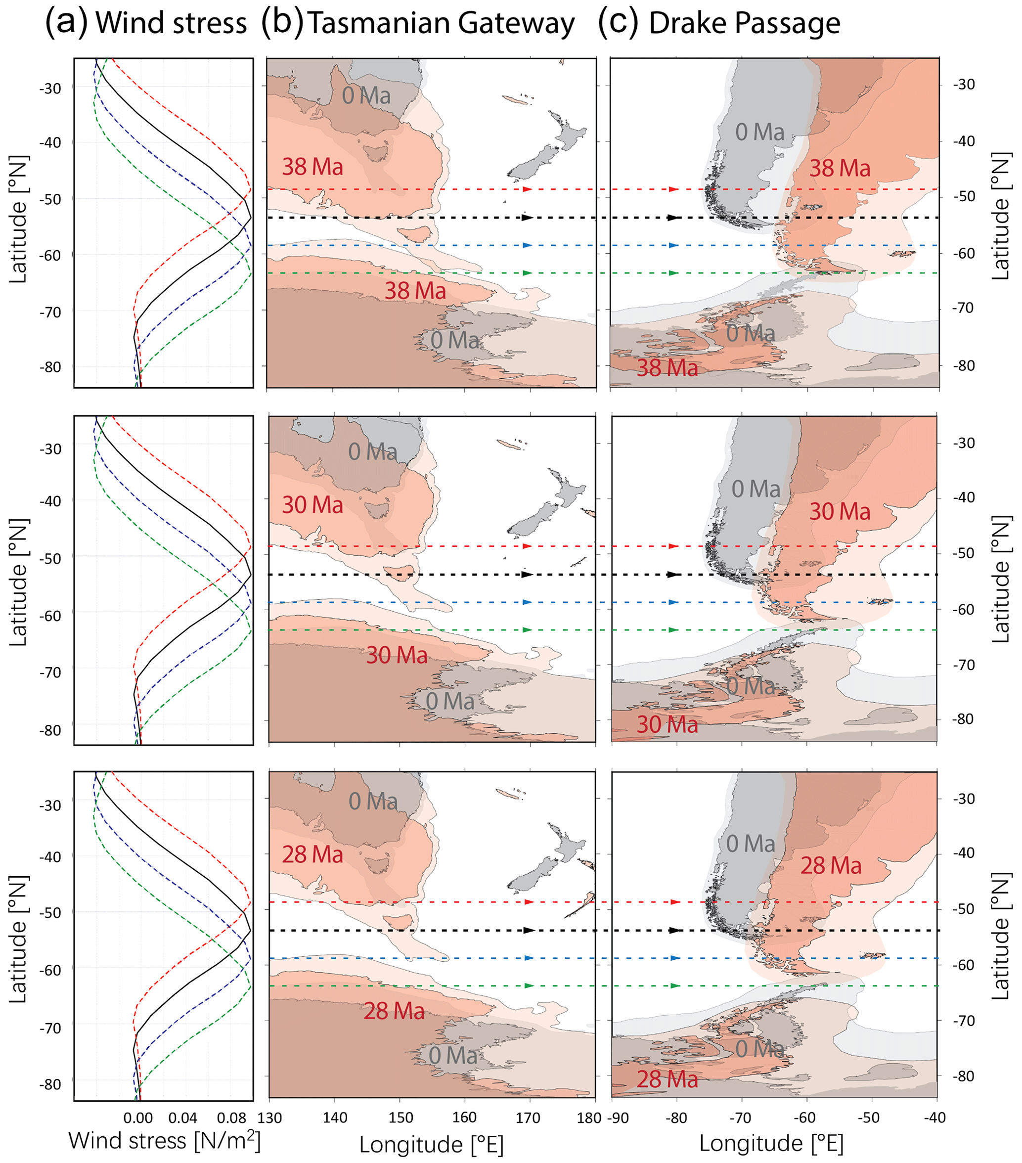
Figure 1(a) Zonal mean wind stresses used in all simulations. The black curve (max 53∘ S) is the revised version from Sauermilch et al. (2021). The maximum westerly of max 53∘ S has a strength of about 0.1 N m−2 and is located at about 53∘ S. Red (max 48∘ S), blue (max 58∘ S) and green (max 63∘ S) curves indicate the shifts of the max 53∘ S curve 5∘ to the north, 5∘ to the south and 10∘ to the south, respectively. Relative positions of continents (at 38, 30, 28 Ma, and present day) versus peak wind stresses for (b) the Tasmania Gateway and (c) the Drake Passage. Coloured dashed lines in (b) and (c) show latitudinal positions of the maximum westerly in four wind stress conditions. Dark orange and grey areas show paleo-continental and modern continental coastlines, respectively. Light orange and light grey areas represent paleo and modern continent-ocean-boundary, respectively. These reconstructions use the rotation model by Matthews et al. (2016) with the paleomagnetic reference frame (van Hinsbergen et al., 2015).
From 38 to 28 Ma, the TG rapidly widened and its paleolatitude changed from 58 to 53∘ S (Fig. 1b). Meanwhile, the northward movement of DP is relatively slow, as its paleolatitude only moved to the north by 1–2∘ from 38 Ma (about 63∘ S) to 28 Ma (about 61∘ S) (Fig. 1b). In order to simulate the consequences of the northward movement of the gateways relative to the wind stress, we adjust the wind stress' paleolatitudes as the input boundary conditions and keep the bathymetric reconstruction fixed. This approach is simpler than changing the framework of the paleo-bathymetric reconstruction in order to adjust the gateways' paleolatitudes.
2.3 Experimental design
The model simulations of Sauermilch et al. (2021) with a TG (DP) depth of 300 m (1000 m) and 1500 m (1000 m) were spun up for over 80 model years. We therefore initialise our experiments from year 86 of Sauermilch et al. (2021). For our reference experiment, we use a smoothed version of the zonal wind stress used in the simulation of Sauermilch et al. (2021). The revised zonally symmetric wind stress has a maximum westerly wind of about 0.1 N m−2 located at 53∘ S and maximum polar easterly wind of about 0.01 N m−2 at 74∘ S (Fig. 1).
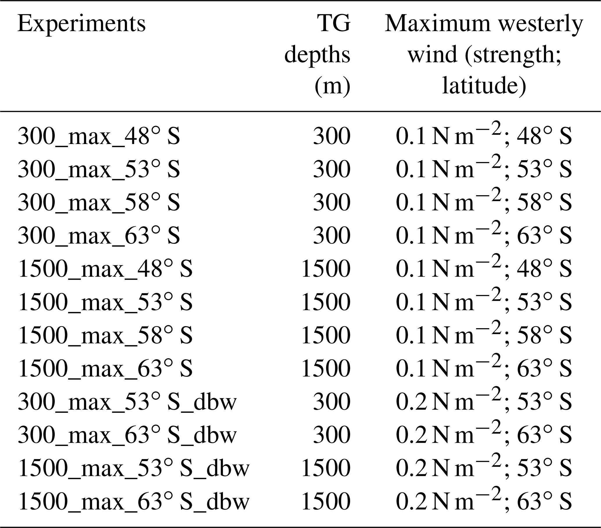
From Fig. 1, we see that the TG had about 5∘ northward movement during the E–O transition. Results from Kennedy et al. (2015) using E–O coupled atmosphere–ocean model indicate that Antarctic ice sheet expansion can cause the shift of westerly wind nearly 10∘ southward. As such, a 5∘ shift in wind stress latitude can indirectly represent the movement of the gateway and a 10∘ a change in the Antarctic ice sheet. This allows us to test the hypothesis of Scher et al. (2015). For our perturbation experiments, we shift the latitude of the wind stress 5∘ to the north, 5∘ to the south and 10∘ to the south (presented as max 48∘ S, max 58∘ S and max 63∘ S, respectively; see Fig. 1a). We conduct eight experiments to test the sensitivity of the Southern Ocean to varied TG depths and wind stress latitudes (see details in Table 1). For example, 1500_max_63∘ S means the case with 1500 m TG and maximum westerly wind located at 63∘ S. Additionally, we double the revised wind stress with the peak wind stress (τm) to about 0.2 N m−2 and use this wind stress in another four cases to test the sensitivity of ocean circulation to changing wind stress (see details in Table 1). All simulations are run for 60 years from the model year 86 of the simulations of Sauermilch et al. (2021). In terms of circumpolar transport, our simulations are well equilibrated (see a time series of zonal transports in Appendix E). Considering the adjustment period of the model due to applying the revised wind stress and shifting or doubling the revised wind stress, we will focus on the final 15 years (model years 130–145) of all the simulations to analyse results.
Table 1Overview of sensitivity experiments. The “experiments” column gives names for each case, e.g. for the 300_max_53∘ S case, 300 represents 300 m TG and max_53∘ S represents the maximum westerly wind of 53∘ S. The“maximum westerly wind” column provides the strength and latitudinal position of maximum westerly wind for each case.
3.1 Sensitivity of Southern Ocean gyres and sea surface temperature to TG depth and wind stress position
Before the inception of the ACC, the early Eocene Southern Ocean basins were dominated by wind-driven gyres that were anti-clockwise for the subtropical gyres and clockwise for the subpolar gyres (Huber et al., 2004; Huber and Nof, 2006; Hill et al., 2013; Hutchinson et al., 2018; Baatsen et al., 2020; Sauermilch et al., 2021). Our control experiment, as shown in Fig. 2c, has a similar circulation. When the TG is 300 m deep, migrations of the wind band adjust the boundaries of the gyres and slightly alter their spatial scale. For example, when the maximum westerly wind peaks at 53∘ S, the boundary between subtropical (red) and subpolar gyres (blue) is also positioned at about 53∘ S. The positional alignment of maximum westerly wind and gyres boundary is consistent with Sverdrup theory. As the latitude of the maximum westerly wind is shifted to 48, 58 and 63∘ S, the gyre's boundary accordingly varies its latitudinal position to 48, 58 and 63∘ S (Fig. 2). Meanwhile, the spatial scale of the subpolar gyre becomes about 30 % smaller for a wind shift from 48 to 63∘ S (Fig. 2a, c, e and g).
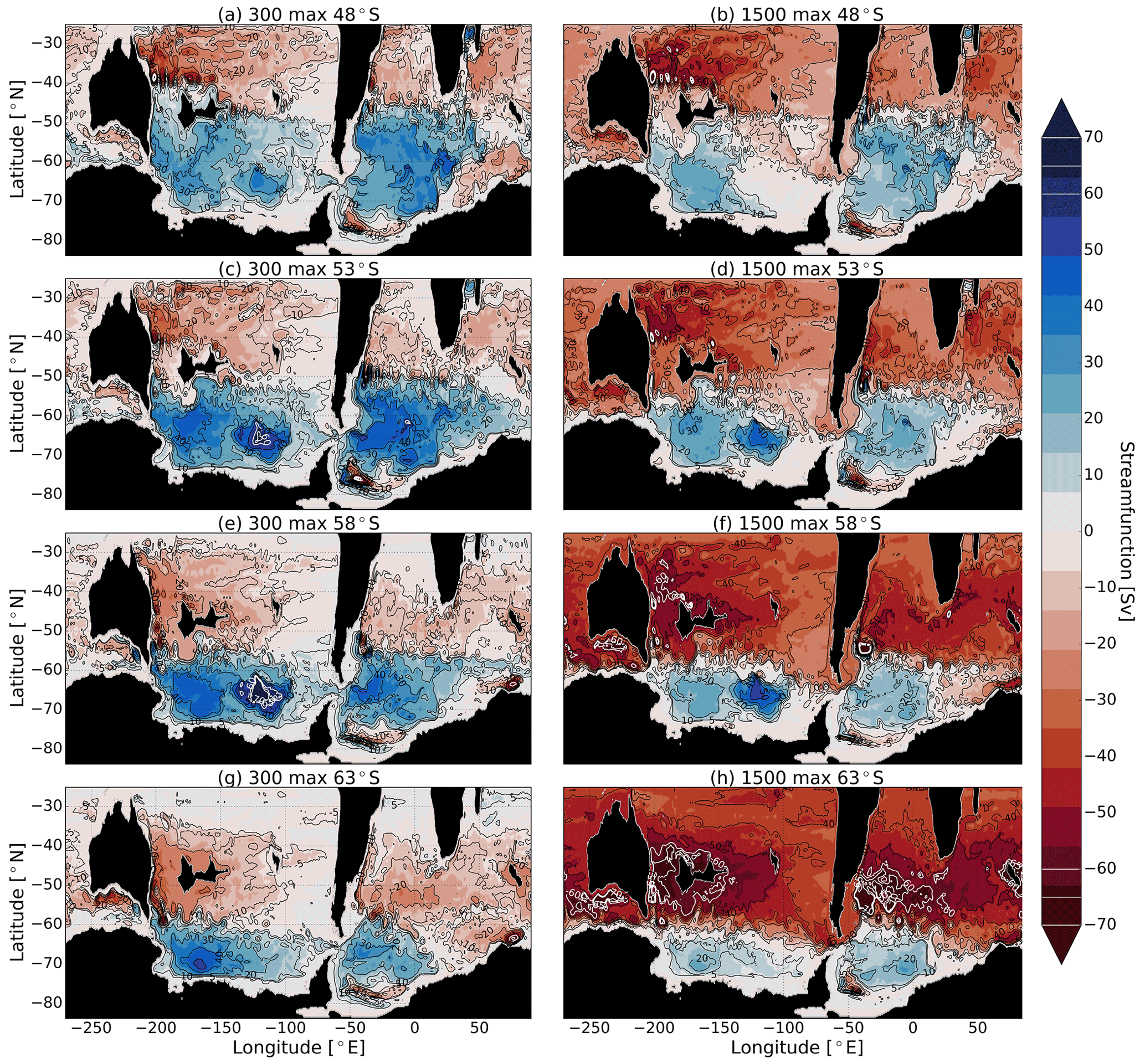
Figure 2The 15-model-year time-average Southern Ocean circulation patterns (annual mean and depth-integrated stream function) under stepwise deepening of the Tasman Gateway from 300 m (a, c, e, g) to 1500 m (b, d, f, h) depth and wind stress meridional migrations (from top to bottom). Red colours indicate anti-clockwise subtropical gyres, and blue colours show clockwise subpolar gyres. The latitudes of τm applied in four cases are 48∘ S (a, b), 53∘ S (c, d), 58∘ S (e, f) and 63∘ S (g, h), respectively. White contours and contour labels at high positive or negative values (−70, −65, −60, 60, 65, 70 Sv) are used to highlight strong streamfunction.
In the simulations of Sauermilch et al. (2021), deepening of the TG to 1500 m results in the subtropical gyres growing and dominating the mid-latitudes of the Southern Ocean. In contrast, the subpolar gyres weaken and shrink. An eastward circumpolar current, with a transport of about 20 Sv, flows through DP (Sauermilch et al., 2021). Our simulations indicate that southward migrations of the wind stress lead to further shrinking of the subpolar gyres (Fig. 2f and h). This change is most remarkable in the 1500_max_63∘ S case, where the northernmost latitude of the subpolar gyres has been restricted to latitudes poleward of 63∘ S. The subpolar gyres shrink over 50 % in area, and the maximum transport decreases to around 10 Sv. The deepening of the TG and southward shifts of the wind stress gradually introduce more circumpolar flow and the establishment of the proto-ACC.
The changes in gyre structure due to wind shifts also induce significant changes in the modelled sea surface temperatures. When the TG is 300 m deep, Sauermilch et al. (2021) show that the colder high-latitudinal waters (about 10–12 ∘C) in the centres of the subpolar Pacific and Atlantic gyres are enclosed by warmer subtropical surface waters (about 15–17 ∘C). The subpolar clockwise gyres transport the subtropical waters to the Antarctic coast. We also present similar temperature patterns with mean sea surface temperatures at high latitudes (higher than 60∘ S) of about 15 ∘C with the shallow TG and maximum westerly wind at 53∘ S (Fig. 3c). The sea surface temperatures with a shallow TG are sensitive to further southward shifts of the westerly wind, as shown in Fig. 3e and g. As the westerly wind moves southward, the warm subtropical water gradually dominates the coastline of Antarctica, and the cold water occupies a smaller and smaller area at the centre of the subpolar gyres. Especially in the model where the TG is 300 m deep and the maximum wind stress is at 63∘ S (Fig. 3g), the cold waters in the Pacific shrink by over 50 % in area. The cold water almost disappears in the South Atlantic, and the mean sea surface temperature at high latitudes increases to about 16 ∘C.
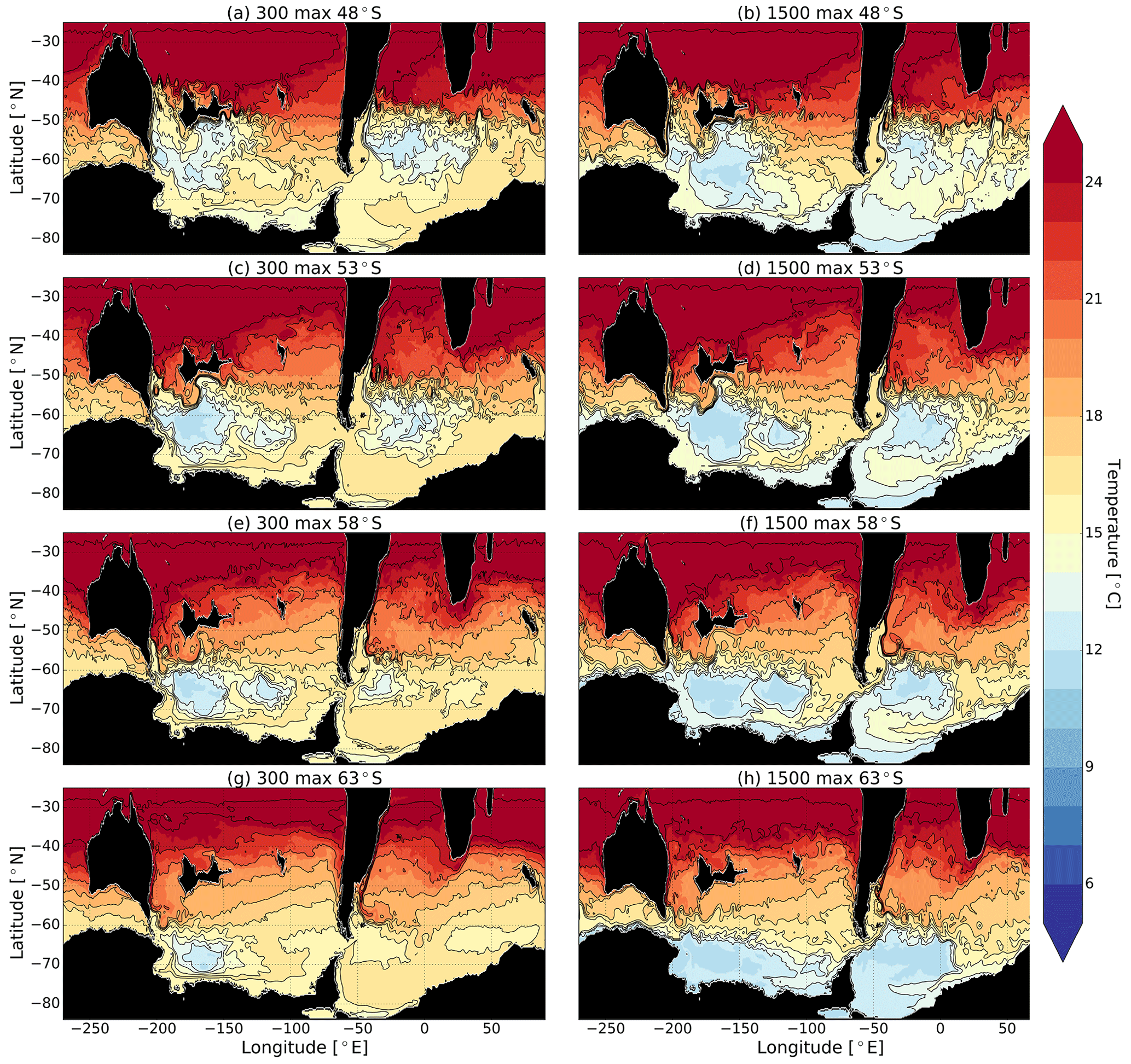
Figure 3Annual mean sea surface temperatures (100 m depth) of the Southern Ocean under the deepening of the Tasman Gateway from 300 m (a, c, e, g) to 1500 m (b, d, f, h) depth and wind stress shifts (from top to bottom).
When the TG is 1500 m deep, the subtropical waters are still able to reach the Antarctic coast and encircle the colder water in the centre of the subpolar gyres when the maximum wind stress is at 48 and 53∘ S. The sea surface temperatures along the Antarctic coast in these two cases are around 15 ∘C (Fig. 3b and d). Therefore, our simulation supports the argument of Sauermilch et al. (2021), who conclude that Antarctica could have been warmed by subtropical waters prior to the E–O transition. However, as the wind stress shifts farther southward (63∘ S), the result is quite different compared to models with a shallow TG. The warm waters from low latitudes gradually fail to reach the polar region (Fig. 3f and h). In the model where the TG is 1500 m deep and the maximum wind stress at 63∘ S (Fig. 3h), the absolute sea surface temperatures along the entire Antarctic coast are lower than 12 ∘C. This leads to the formation of a large meridional temperature gradient across the Southern Ocean. This allows a strong eastward geostrophic current, resembling the modern ACC, to form and be sustained via thermal wind shear. This proto-ACC impedes the warm subtropical waters reaching high latitudes and allows the cooler subpolar waters to thermally isolate the Antarctic continent.
To explore the how ocean transport sustains the warm SST, the zonally and vertically integrated meridional heat transport (MHT) is calculated for four cases: 300_max_53∘ S, 300_max_63∘ S, 1500_max_53∘ S and 1500_max_63∘ S due to the significant changes in streamfunction and sea surface temperature between these cases (Fig. 4). The calculation of the MHT is based on that of Bryan (1982), i.e. zonally and vertically integrating the product of the meridional velocity and potential temperature.
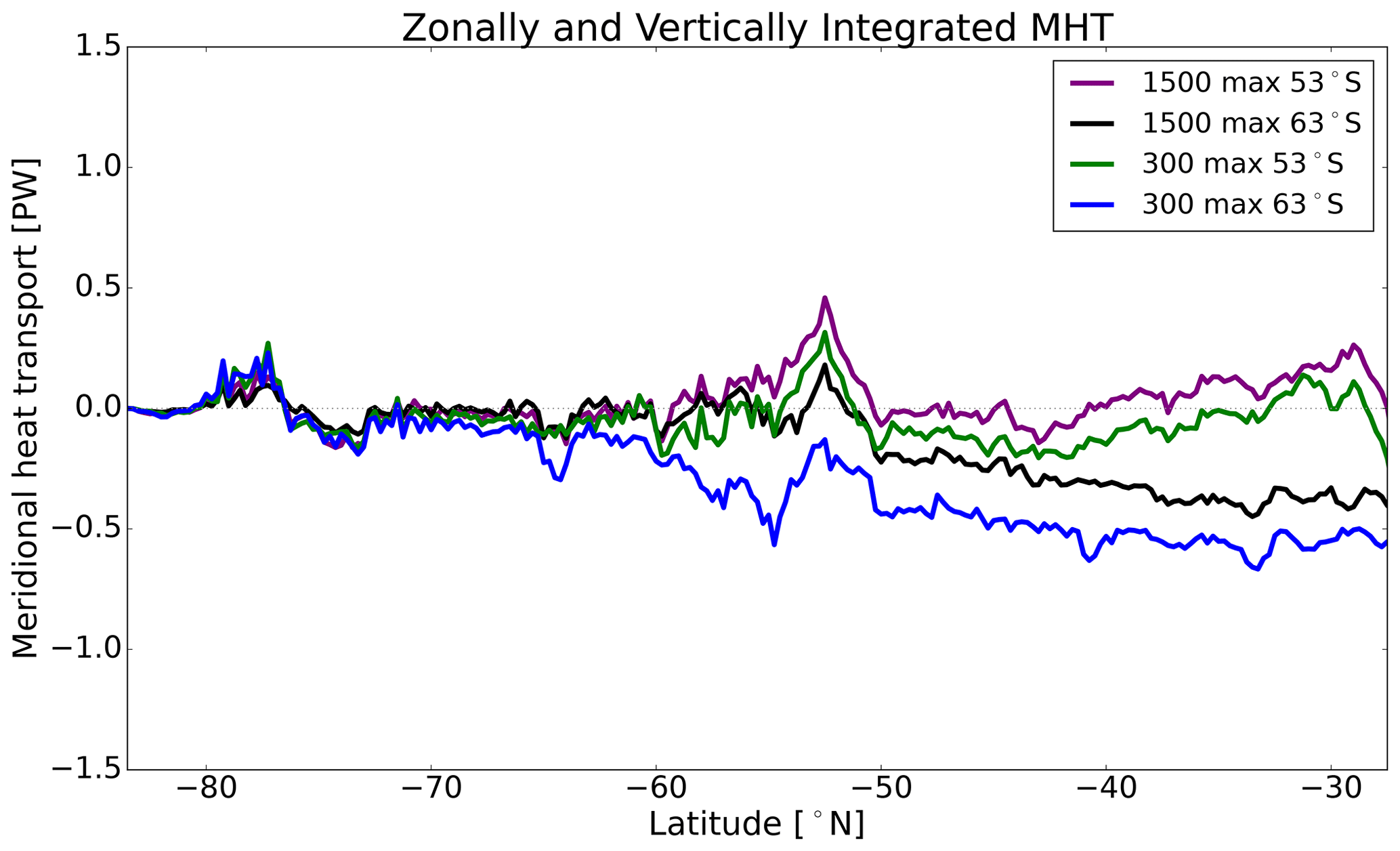
Figure 4Zonally and vertically integrated meridional heat transport (MHT; in PW) for 300_max_53∘ S (green), 1500_max_53∘ S (purple), 300_max_63∘ S (blue) and 1500_max_63∘ S (black). Note that the domain north of 27.5∘ S is manually removed to avoid the impact of the restoring near the northern boundary.
South of 50∘ S is roughly where the sharp temperature gradient and transition from gyre to circumpolar flow occurs. As shown in Fig. 4, the convergence of heat south of 50∘ S in the 300_max_63∘ S case is typically higher than the other cases. This indicates that the ocean transports more heat into this region and sustains higher temperatures. Corresponding to this, the domain average sea surface temperature of the 300_max_63∘ S case is higher than other three cases. In contrast, the 1500_max_63∘ S case has the weakest southward MHT, thus the minimal heat convergence south of 50∘ S. This is due to the strongest circumpolar current blocking gyre-driven heat advection. The two cases with the westerly wind peak at 53∘ S also both show very weak heat convergence south of 50∘ S. This may be associated with the larger subpolar gyres, allowing the strong western boundary current to transport heat northward so that the southward MHT is offset.
Table 2Net TG and DP throughflow volume transport (Sv). Positive values indicate eastward transport, and negative values present westward transport. All values are the annual mean transport of the final 15 years of the simulations.

3.2 Response of throughflow transport to doubling wind stress
The maximum zonal volume transport through each gateway does not exceed 50 Sv (TG transport: 47.9 Sv; DP transport: 38.3 Sv; Table 2, 1500_max_63∘ S), which is about a third of the modern-strength ACC (transport of 137 Sv; Meredith et al., 2011). In the traditional paradigm, wind stress acts as an important driver of ocean currents. Thus, increased wind stress is expected to strengthen the input of zonal momentum to the ocean and accelerate ocean currents. We simulate the consequences of doubling the wind stress (from 0.1 to 0.2 N m−2) with different gateway depths (TG at 300, 1500 m) and different latitudinal positions of maximum wind stress (at 53 and 63∘ S). The variations of the TG and DP transport are shown in Table 2 and Fig. 5.
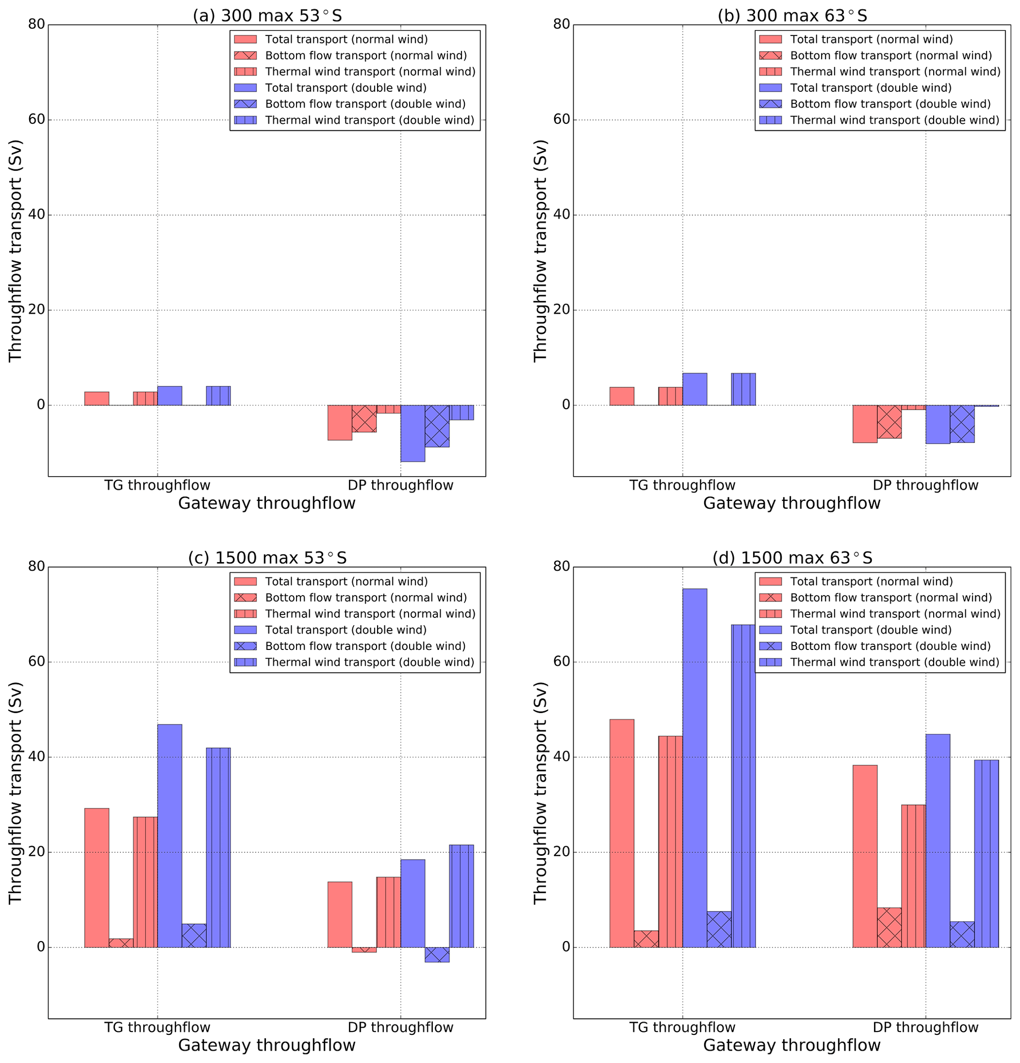
Figure 5The contrast of TG (red) and DP (blue) throughflow volume transport in normal-strength and double-strength wind stress experiments. The total transport (Ttotal) is decomposed into bottom flow transport (Tb) and thermal wind transport (Ttw).
The total TG transport is strengthened in all four simulations due to the doubled westerly wind stress. When TG is 300 m, TG transport increases 43 % and 72 %, with peak wind stress located at 53 and 63∘ S, respectively. Note that the TG transport is small, and its change due to doubled wind stress is also small in an absolute sense when TG is 300 m. As a result, these large percentages may not be physically important. When the TG is 1500 m, TG transport is increased by 60 % and 57 % with peak wind stress located at 53 and 63∘ S, respectively. The effect is particularly strong when the maximum wind strength is at 63∘ S, which gives a TG transport of 75.4 Sv. Conversely, the total DP transport is not strongly influenced by the changes in wind stress with the increases in most simulations lower than 35 %.
In a homogenous ocean, currents are strongly constrained by contours, where f is the Coriolis parameter and H is the ocean depth (Johnson and Hill, 1975). Even in the presence of stratification, the bathymetry and continents of the Southern Ocean can block contours, which steers the current to maintain conservation of potential vorticity (Marshall, 1995). The blocking of contours reduces the velocity below the bathymetric level and allows the transport due to thermal wind shear to dominate the ocean current transport (Munday et al., 2015). Given the complex paleo-bathymetry applied in this model study, we decompose the total TG/DP transport into two components contributed by bottom flow transport Tb (transport below a chosen bathymetric level) and thermal wind transport Ttw (transport above the chosen bathymetric level) using three equations:
Equation (4) calculates the zonal bottom flow velocity Ub. By examining hydrographic sections of the local bathymetry and zonal velocity (see the example of TG in Appendix F and Fig. F1), we select a model level below which the current velocities have little vertical and meridional gradient (shear). This allows a clean separation of the flow that is due to thermal wind shear and that which is not. The vertical average of zonal velocity below the chosen model level is then used as the Ub. In the shallow TG cases, e.g. the 300_max_53∘ S case, we choose model level 30 (446 m). In the deep TG cases, e.g. the 1500_max_53∘ S case, we select model level 32 (668 m). In all cases, we select the model level 33 (728 m) for the DP. Equations (5) and (6) calculate the bottom flow transport and thermal wind transport, as per Eqs. (4) and (5) in Munday et al. (2015).
With a 300 m TG (Fig. 5a and b), Ttw dominates the entire TG transport, while the DP transport is dominated by a westward bottom flow (negative Tb). Both Ttw and Tb for each gateway are small in the case of a 300 m TG (<4 Sv for TG and <9 Sv westward for DP). The response of Tb and Ttw to doubling wind stress is also shown in Fig. 5. Both latitudinal shifts and doubling of the wind stress cannot increase the TG transport (Ttotal, Ttw and Tb) to larger than 7 Sv and the DP westward transport (Ttotal, Ttw and Tb) to larger than 12 Sv with a 300 m TG.
When the TG deepens to 1500 m (Fig. 5c and d), the deeper bathymetry allows for the generation of a strong bottom flow (Tb) through the TG. Doubling wind stress strengthens the Tb through the TG significantly (89 % and 77 % increase when peak wind stress is located at 53 and 63∘ S, respectively), while changes in Ttw through the TG due to doubled wind stress are small (16 % and 18 % when peak wind stress is located at 53 and 63∘ S, respectively).
With the deeper TG, a big variation occurs in the dominance of DP transport, changing from Tb to Ttw. Both components of DP transport are less sensitive to the doubling wind stress (21 % and 15 % increase for Tb and Ttw, respectively) with the peak wind stress located at 63∘ S. In addition, the following two points are noticeable: (1) the Tb through the DP is still negative in the 1500_max_53∘ S case, which means that the westward bottom flow through the DP still exists with a deep TG and maximum westerly wind located at 53∘ S, and (2) in the 1500_max_63∘ S case, the DP bottom flow is now eastward, but its transport weakens with doubling wind stress.
3.3 Topographic form stress in the late Eocene Southern Ocean
The modern Southern Ocean does not have any continental barriers in the latitudes of the DP to support a pressure gradient and balance the momentum input by the wind. The continents of the late Eocene Southern Ocean are present at the latitudes of the TG and DP. This may influence the momentum balance in the Southern Ocean and evolution of the proto-ACC. With realistic bathymetry of the late Eocene Southern Ocean, it is necessary to consider the pressure gradients across continents or landmasses in the momentum balance. Masich et al. (2015) calculate pressure gradients across both continents and submerged topography, constituting the total topographic form stress, in the Southern Ocean State Estimate (SOSE, Mazloff et al., 2010). They depict its balance with zonal wind stress in the modern ACC latitudes. Following Masich et al. (2015), we first derive the zonally and vertically integrated momentum balance in the late Eocene Southern Ocean (see Appendix A). We then extract the total topographic form stress and analyse how its depth and meridional structure reflect the circulation and dynamics of the Eocene Southern Ocean. More detail on the calculation of topographic form stress and errors associated with the use of partial model cells can be found in Appendices B and C.
Previous studies have described different regimes in the topographic form stress for the modern Southern Ocean at different depths (Gille, 1997; Grezio et al., 2005; Masich et al., 2015). Nevertheless, the different bathymetry of the late Eocene Southern Ocean may change the modern picture. In addition, the shallower and narrower gateways of the Eocene may impact the momentum balance and topographic form stress by allowing the continents to play a larger role in balancing wind stress. This could influence the circumpolar transport's sensitivity to wind stress in the Eocene ocean.
To determine how topographic form stress and wind stress balance in the context of late Eocene Southern Ocean and in the different vertical regimes, we horizontally integrate and vertically accumulate the topographic form stress and wind stress downwards from the surface to every depth, the comparison of which is shown in Fig. 6. Generally, the depth-integrated topographic form stress contributions in the four cases have similar variation. Near the sea surface, the topographic form stress signal is positive and reaches a maximum value at a shallow depth (Hs, e.g. 380 m in the 1500_max_53∘ S case). The surface or upper layer of the Southern Ocean has few submerged bathymetric features, meaning that the pressure gradient across continents must be the primary source of topographic form stress. In these upper layers, the continents are pushing in the same direction as the wind stress. Below the near-surface layer, the signal decreases in magnitude until a mid-depth layer(Hm, e.g. 610 m in the 1500_max_53∘ S case) where the integrated topographic form stress is zero. In this layer, the initial eastward push from the topographic form stress has been matched by a corresponding westward push, such that they cancel each other out at Hm. At this depth, the continents exert zero net push on the ocean. Finally, below Hm the depth-integrated topographic form stress is increasingly negative to the ocean floor. This deep layer is where the bathymetry pushes back and balances the wind. At deep depths (Hd, e.g. 3880 m in the 1500_max_53∘ S case), the integrated topographic form stress is of sufficient magnitude to balance the wind stress.
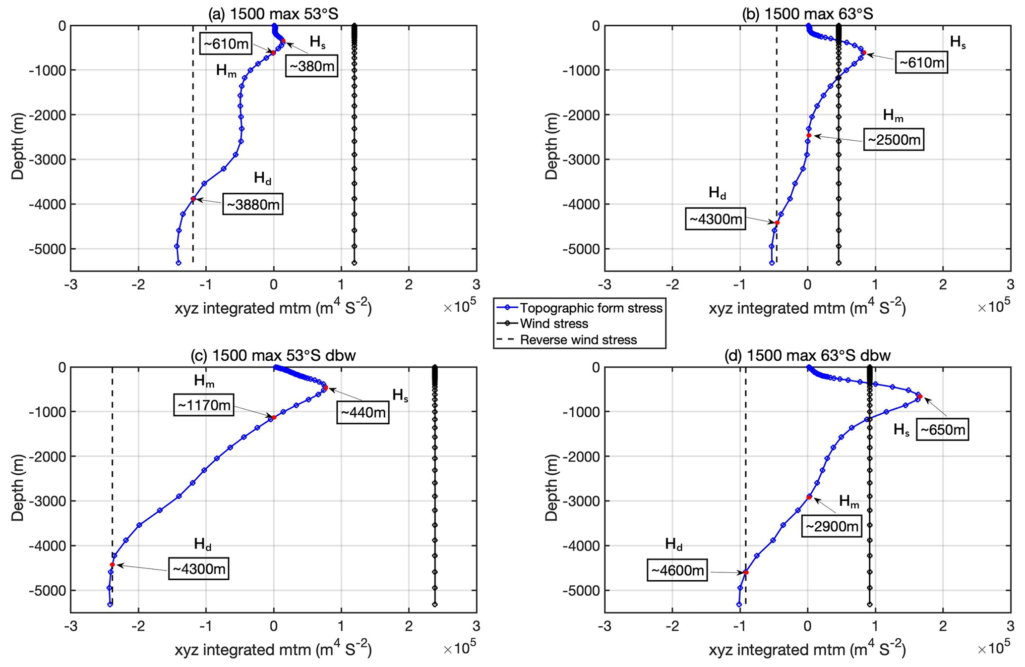
Figure 6The comparison of horizontally integrated and vertically accumulated topographic form stress and wind stress in 1500_max_53∘ S (a), 1500_max_63∘ S (b), 1500_max_53∘ S_dbw (c) and 1500_max_63∘ S_dbw (d) cases. The blue curve is the topographic form stress integrated from surface to various depths. The black line is the wind stress integrated from surface to various depths. The dashed line is the reversed wind stress integrated from surface to various depths (the same strength but opposite sign compared to depth-integrated wind stress). There are three unique depths indicated by red points in all four cases. The shallow depth (Hs) is the first local maximum in the depth-integrated topographic form stress, which has the same sign as the integrated wind stress (e.g. 380 m in a). The mid-depth layer (Hm) is where depth-integrated topographic form stress is zero (e.g. 610 m in a). The deep depth layer (Hd) is where the depth-integrated topographic form stress intersects with reverse wind stress or has the same contribution but opposite sign compared to depth-integrated wind stress (e.g. 3880 m in a).
By comparing with the reconstructed paleo-bathymetry (Fig. D1a) used in all simulations, we see that Hs probably corresponds to continental shelves in some regions, like northern Australia, South America and Antarctica. Hm in the cases at 53∘ S is probably controlled by the tops of seamounts in the north of New Zealand and south-east of Africa. In the 63∘ S cases, Hm may be associated with the top of mid-ocean ridges in the circumpolar belt. Finally, Hd may correspond to the subduction zone of the mid-ocean ridge.
Dividing the ocean into latitude bands can highlight changes in the depth-integrated topographic form stress signal (Masich et al., 2015). We divide our model domain into three latitude bands by considering the ocean circulation and bathymetry. These bands are the northern region (northern; 25–50∘ S), the circumpolar belt (middle; 50–70∘ S), and the polar region (polar; 70–83∘ S). These three regions have different surface ocean areas due to the change in the longitudinal extent of the Earth with latitude and the position of the continents. As such, we normalise the depth-integrated topographic form stress and wind stress by surface ocean area in the three regions.
From Fig. 7, we can see that the northern region in all cases has a positive depth-integrated topographic form stress signal (green curve) near the ocean surface, as with the full domain signal in Fig. 6. This signal reaches a maximum around Hs. This suggests that it is the subtropical gyres of the northern region that are responsible for these shallow maxima. Below Hs, the pressure gradient across submerged topography acts to cancel the positive signal. When the peak westerly wind is at 53∘ S, the wind stress in the northern region is positive (westerly wind dominates). As the peak westerly wind shifts from 53 to 63∘ S, the wind stress contribution in the northern region changes sign from positive to negative. The gyres are still able to form because they depend upon the curl of the wind rather than its direction (Stommel, 1948; Munk, 1950). However, the vertical structure of the topographic form stress is characteristically different to the 53∘ S wind stress cases because it must remain positive at depth to balance a westward wind stress. In the meantime, the subtropical easterlies dominate the northern region, and the subtropical gyre expands in size.
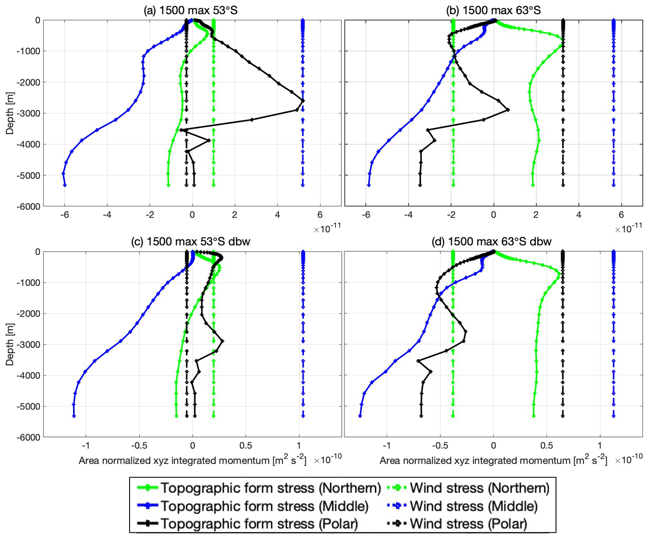
Figure 7Area-normalised depth-integrated topographic form stress (solid curve) and wind stress integrated from the surface to various depths (dashed black line) in three channels (northern: 25–50∘ S, green; middle: 50–70∘ S, blue; polar: 70–83∘ S, black).
In the circumpolar belt, all panels in Fig. 7 show a consistently negative depth-integrated topographic form stress. This acts to balance the eastward wind stress at Hd. This is the signal of circumpolar flow with the surface wind stress balanced by bottom form stress via vertical flux of momentum by mesoscale eddies. This balance prevails in the modern Southern Ocean (Johnson and Bryden, 1989; Ward and Hogg, 2011). It is this region that dominates the whole-ocean momentum balances at depth.
In the polar region, we find a positive topographic form stress signal above 3800 m in the 53∘ S cases. This is balancing a net westward wind stress and has a similar vertical structure to that noted for the northern region above. This may indicate a characteristic contribution of the subpolar gyre. The positive topographic form stress signal is not present in the 63∘ S cases. The change in structure of the wind results in a net eastward wind stress in these experiments. As such, the topographic form stress must become negative. However, the vertical structure has a tendency towards more negative values at depth, rather than variation around the value that balances the wind stress seen in Fig. 7b and c. This is probably induced by the shrinkage of the subpolar gyre and the inception or strengthening of the proto-ACC, which intrudes into this latitude band and influences its momentum balance.
Almost all submerged topographic features in our model have bathymetry deeper than Hs (see the reconstructed paleo-bathymetry in Appendix C). Hence, Hs can be recognised as a contribution-dividing depth, above which the topographic form stress is the contribution largely sustained by the pressure gradient across continents and below which the topographic form stress is contributed by submerged topography and the rest of continents. We apply Hs, which is allowed to vary between experiments, to decompose the total topographic form stress into shallow (shallow TFS) and deep topographic form stress (deep TFS). The model level Hs is applied in the Eq. (B3) to give shallow or deep topographic form stress contributions.
Figure 8 shows that the subtropical easterly wind stress is mostly balanced by the shallow TFS contribution (positive sign). Comparing with the results shown in Figs. 6 and 7, the positive signal of the depth-integrated topographic form stress in the upper regime (e.g. above 610 m in Fig. 6d) and in the northern region is mostly contributed by shallow TFS. This is generated by the subtropical gyres in the surface layer to cancel the momentum input from subtropical easterly wind stress (Fig. 8d). All panels in Fig. 8 also show that the westerly wind stress is largely balanced by deep TFS (negative sign), which is caused by the eastward current (e.g. proto-ACC) flowing across submerged topography and mostly contributes to the negative signal of the depth-integrated topographic form stress in the circumpolar belt.
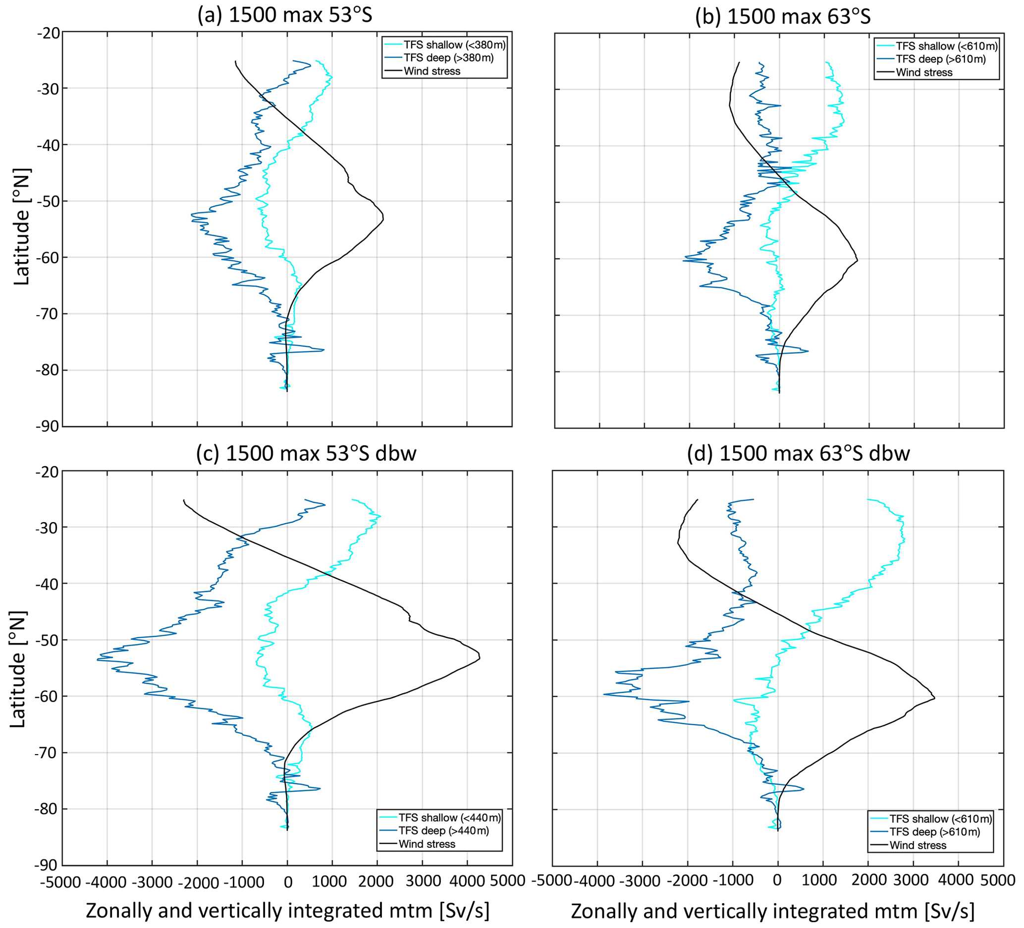
Figure 8The zonally and vertically integrated momentum budget between wind stress (black; Sv s−1), shallow topographic form stress (light blue; Sv s−1) and deep topographic form stress (dark blue; Sv s−1) in the 1500_max_53∘ S, 1500_max_63∘ S, 1500_max_53∘ S_dbw and 1500_max_63∘ S_dbw cases.
In the 1500_max_53∘ S case (Fig. 8a), the deep TFS has some positive signals to balance the easterly wind stress in the latitudes of 25 to 29∘ S. In comparison, in the 1500_max_63∘ S case, the deep TFS at these latitudes is negative (Fig. 8b). The maximum positive signal of the depth-integrated topographic form stress at Hs in the 1500_max_63∘ S case is larger than depth-integrated wind stress (Fig. 6b). This is due to the large shallow TFS contribution in the latitudes of the northern region, which is then balanced with both wind stress and deep TFS. A weak positive signal of shallow TFS occurs in the latitudes of 60 to 75∘ S in the 1500_max_53∘ S case but disappears in the 1500_max_63∘ S case (Fig. 8a and b), which may be related to the inception of the proto-ACC. With double-strength wind conditions (0.2 N m−2; Fig. 8c and d), the sensitivity of the shallow TFS to doubled wind is strong in the latitudes of subtropical easterlies, whereas it is weak in the latitudes of westerlies. The deep TFS shows consistently strong sensitivity in all latitudes. The sensitivity or insensitivity of the shallow and deep TFS is associated with the responses of TG and DP transport to doubled wind stress, which will be discussed in the following section.
4.1 Uncertainties of model configuration
This study is aimed at modelling the late Eocene Southern Ocean with realistic paleo-bathymetry. Coupled atmosphere–ocean models, such as Huber and Nof (2006), Sijp and England (2004); Sijp et al. (2011), and Hill et al. (2013), usually have low-resolution ocean components. This limits their representation of ocean circulation and dynamics and also impacts their ability to precisely represent the detail of the sea floor. The supplementary information of Sauermilch et al. (2021) shows that changing resolution or bathymetry has a large impact on the model results, such as modifying the SST distribution, ocean heat transport, the strength and size of gyres, and the inception of the proto-ACC. Given our focus on ocean dynamics in this study, we have chosen to restrict ourselves to an ∘ ocean-only model in order to partially resolve the eddy field.
Typically, the literature considers ∘ grid spacing to be eddy-permitting spacing and –∘ to be eddy-resolving spacing (Delworth et al., 2012; Hallberg, 2013; Mecking et al., 2016; Megann, 2018). In addition, the grid spacing of our model at 60∘ S is about 12.5 km. Given that eddies are typically several multiples of the deformation radius when fully mature, this puts our model firmly in the eddy-permitting category. The domain surface average eddy kinetic energy (EKE) of the 1500_max_53∘ S is around 0.003 m2 s2, which is lower than the surface average EKE (0.012 m2 s2) in the ∘ Southern Ocean model of Munday et al. (2021). Given that ocean models with ∘ grid spacing typically have about half the eddy kinetic energy of the modern Southern Ocean as measured by satellite altimetry (Delworth et al., 2012; Spence et al., 2012), this implies that our model simulation probably underestimates the EKE of real late Eocene Southern Ocean.
The compromise of using an ocean-only model requires removing some key feedbacks in the configuration. For example, the implementation of the restoring is based on Haney (1971), acting as a low-order approximation to the energy balance at the surface of the ocean. The intention is to effectively mimic the strong restoring of the SST to an overlying atmospheric temperature. This study sets restoring time for SST and SSS to 10 d, which is a fairly standard restoring time for SST due to the strong feedback between SST and surface heat flux. This is quite a short timescale for salinity restoring due to it only presenting a weak feedback between SSS and evaporation and precipitation. However, this study's aim of using 10 d for both temperature and salinity is to ensure a good fit to SST and SSS fields of Hutchinson et al. (2018).
In general, a short restoring timescale in the model tends to lead to higher fluxes and acts to damp surface variance in temperature and salinity, as well as eddy kinetic energy (Zhai and Munday, 2014). As shown by Zhai and Munday (2014), strong surface restoring makes the isopycnal slopes less sensitive to wind stress than for a purely flux condition. This implies that the thermal wind transport is also less sensitive to wind stress than might otherwise be the case, since it is strongly linked to isopycnal slope. In our study, the thermal wind transport is the majority of the zonal flow through TG and DP. Therefore, the sensitivity of TG and DP transport in this study is probably lower than zonal flow transport in a model using a pure flux condition on temperature and salinity or bulk formula to calculate the heat fluxes from atmospheric temperature.
Our bathymetric reconstruction uses the plate rotation model (Matthews et al., 2016) with a paleomagnetic reference frame (van Hinsbergen et al., 2015). We note that there can be a range of uncertainties regarding the absolute location of the geographical constellation of continents. This particularly affects the latitudinal positions of the key gateways, depending on the choice of the plate tectonic model and reference frame. This can have significant consequences for the results of the ocean model simulations (e.g. Baatsen et al., 2018). However, as our paleo-bathymetry uses the same plate tectonic setup (model, reference frame) as the bathymetry used by the coupled climate model that provides the surface forcing (Hutchinson et al., 2018), we expect our model simulations to at least be internally consistent.
As noted earlier, the TG moved northward by 5∘ and DP by 1–2∘ between 38 and 28 Ma (Fig. 1). Very little information exists about the impact of Antarctic cooling, especially Antarctic ice sheet (AIS) expansion, on the latitudinal position of the westerly wind. However, results from an E–O coupled atmosphere–ocean model indicate that the westerly wind shifts nearly 10∘ southward, with the appearance of AIS (Kennedy et al., 2015). Assuming a westerly wind (peak wind stress located at 53∘ S) shift southward by 10∘ at 34 Ma and that the TG and DP move northward by 5 and 1–2∘, respectively, around the same period (from 38 to 28 Ma), it is likely that around 28 Ma the gateways and wind maximum show the best latitudinal alignment. This alignment is probably important for the inception of strong proto-ACC, which is discussed in the Sect. 4.2.
4.2 Prerequisite for the inception of proto-ACC
Our results show that with a shallow TG (300 m), the maximum TG transport is only 3.9 Sv with the maximum wind stress at 63∘ S (Table 2). Meanwhile, the opening of the DP (1000 m) allows a negative net DP transport, leading to a westward flow from the Atlantic to the Pacific (Table 2), which is associated with circulation between subpolar gyres in the Atlantic and Pacific. This suggests that a strong proto-ACC may not be possible while the TG is shallow even if the wind stress maximum is aligned with the TG. Some studies use numerical models (Sijp et al., 2011) or proxies (Stickley et al., 2004) to infer that a deep TG allows a strong throughflow as part of the formation of the proto-ACC. However, our 1500_max_53∘ S case (1500 m TG and 1000 m DP) only simulates a 29.3 Sv TG transport and a 13.8 Sv DP transport. At the same time, the subpolar gyres are still vigorous (maximum transport streamfunction 40 Sv) enough to transport warm subtropical waters to reach Antarctic. Hence, the TG deepening can induce an eastward TG throughflow as an initial phase of a proto-ACC. However, other conditions for the development of a strong proto-ACC that is capable of contributing to the observed changes to the E–O Southern Ocean circulation and climate may be necessary.
In addition to the impact of TG deepening on the onset of the proto-ACC, we should also consider the role of the meridional position of the wind stress maximum. Our model shows a stronger proto-ACC (TG transport ∼47.9 Sv, DP transport ∼38.3 Sv; Table 2) in the 1500_max_63∘ S case, in which the maximum westerly wind stress is aligned with both the TG and the DP. With a 1500 m TG, the strong TG throughflow invades the subpolar Pacific sector, forming a large-scale eastward ocean current broadly along the latitude of the maximum westerly wind. This current extends downstream towards the DP. Once the eastward current reaches around the tip of South America, its following pathway is quite distinct in different wind stress cases. For instance, when the maximum westerly wind is at 53 or 58∘ S, the continental barrier forces the eastward current to flow poleward and then mostly to reform into subpolar gyres.
If carefully comparing the latitudes of different wind stresses and both gateways at 38 Ma (Fig. 1), we find that the maximum westerly wind of 63∘ S is at the southern margin of the TG and the northern margin of the DP. This condition enables the eastward current to mostly penetrate the DP without turning poleward to replenish the subpolar gyres. Thus, the latitudinal alignment of deep gateways (TG and DP) and the maximum westerly wind may be a prerequisite for the inception of a strong proto-ACC and the cooling of the late Eocene Southern Ocean. This suggests that the hypothesis of Scher et al. (2015) may well be correct, answering our question in Sect. 1.2. Regarding the alignment of wind stress with TG and DP, a interesting question is raised for future work: what are the impacts of applying a wind stress that is not zonally symmetric in the model configuration for the inception of proto-ACC?
4.3 Sensitivity/insensitivity of proto-ACC to doubled wind stress
The proto-ACC transport in our 1500_max_63∘ S case (TG transport: 47.9 Sv; DP transport: 38.3 Sv) is only about 30 % of the modern ACC transport. Our experiments using a doubled wind stress (1500_max_63∘ S_dbw case) produce a more vigorous proto-ACC, with a TG transport of 75.4 Sv and a DP transport of 44.8 Sv (Table 2). We find that the TG throughflow is strengthened significantly but not doubled with doubled wind stress (the increase is 57 %). In contrast, the DP transport is relatively insensitive to an increase in wind strength, with the increase being only 16 %. This may be due to eddy saturation (see Sect. 1.2), which has been found in many models of the Southern Ocean.
Munday et al. (2013) have proposed that the ocean model with finer resolution will significantly reduce the sensitivity of circumpolar transport to wind stress compared to an eddy-permitting model. They even demonstrate zero sensitivity of their model's circumpolar transport to wind stress due to strong eddy activity in an eddy-resolving model. Our experiments show a less eddy-saturated result in the TG and DP transport, which may be due in part to our eddy-permitting model and its incomplete representation of mesoscale eddies. In addition, the width of the TG or DP in our simulation is much narrower than in the modern world. This may contribute to the change in eddy saturation due to interactions between the flow and bathymetry.
Our study finds that the responses of TG or DP transport to doubled wind stress are significantly different. Similarly, Munday et al. (2015) observe the insensitivity of circumpolar transport with only a bathymetric ridge in an idealised eddy-permitting model. The addition of continental barriers into channels with a single ridge high enough to block contours reintroduces the sensitivity of circumpolar transport at low winds when their peak wind stress is below 0.2 N m−2 (Munday et al., 2015). They analyse the zonal momentum budget and argue that the continental form stress may dominate the role of bottom form stress in the momentum balance with the introduction of continental obstacles (Munday et al., 2015). The continents exert their pressure gradient across all depths and push back against the mean flow so that the vertical eddy transport of momentum is bypassed and the circumpolar transport is dependent upon the wind. Hence, the difference in the sensitivity of the proto-ACC's transport through the TG or DP may be associated with the changes in some dominant terms of the zonal momentum budget.
In our simulations, we can interpret sensitivity or insensitivity of the TG and DP transport via the momentum balance between wind stress and topographic form stress, which itself may respond to wind stress changes. The TG transport is dominated by subtropical gyres that sustain the shallow TFS in the circumpolar belt and which does not respond to changes in wind strength. Therefore, this shallow TFS cannot adequately balance the doubled momentum input from wind stress, which acts to accelerate or strengthen the TG throughflow so that the TG transport is relatively sensitive to the doubled wind stress. In contrast, the complicated submerged bathymetry in the DP region allows the DP throughflow to generate a deep TFS that responds strongly to changes in wind stress due to vertical transmission by eddy form stresses. This deep TFS is expected to balance the wind stress, break the connection between mean flow and wind stress, and allow strong eddy saturation of the DP transport. Overall, we expect that there will be a strong sensitivity of the associated gateway throughflow and transport to changes in wind stress when the form stress that balances the wind is dependent upon the mean flow. In contrast, when the form stress is instead dependent upon transient features, i.e. eddies, there is weak sensitivity of the gateway throughflow and transport to the imposed wind stress, and thus an eddy-saturated state can result.
In terms of transport across the TG and DP and their sensitivities to changing wind stress, future work can be conducted to investigate whether the latitudinal offset of TG and DP can play an important role in the zonal transport and momentum balance.
Early studies proposed a connection between the opening and deepening of tectonic gateways linking the main basins of the Southern Ocean and changes in E–O oceanographic circulation patterns (Kennett, 1977; Murphy and Kennett, 1986; Toggweiler and Bjornsson, 2000; Huber et al., 2004; Sijp and England, 2004; Stickley et al., 2004). Recent studies further show the important role of the gateways' opening and deepening and wind stress in the changes of Southern Ocean gyres and the development of the ACC (Munday et al., 2015; Scher et al., 2015; Sauermilch et al., 2021). Here we use a high-resolution ocean model with a realistic paleo-bathymetry to investigate the sensitivity of the E–O Southern Ocean to TG deepening and changing wind stress. This study also analyses the zonal momentum budget of the Southern Ocean to interpret the simulated dynamics. Some of the key findings are as follows.
-
In the E–O Southern Ocean, southward shifts of wind stress expand the size of subtropical gyres and shrink the size of subpolar gyres.
-
When the TG is shallow (300 m), the migration of wind stress does not cause major changes in ocean gyres and SSTs. When the TG is deep (1500 m), only the latitudinal alignment of the maximum westerly wind with both the TG and the DP leads to a strong increase in proto-ACC transport and hence the cooling of the Eocene Southern Ocean.
-
The momentum input from doubled wind stress leads to a large increase in the proto-ACC transport through the TG, while the response of the transport through the DP is weak.
-
Subtropical gyres sustain the positive topographic form stress (the same direction with wind stress) near the ocean surface (<700 m). The momentum balance between wind stress and topographic form stress occurs at depth (>3800 m) to support the strong proto-ACC in the circumpolar belt (50–70∘ S).
The zonal momentum equation is given by
where u is zonal velocity, ub is zonal velocity in the bottom level, ξ is the vertical component of the relative vorticity, v is meridional velocity, w is vertical velocity, f is the Coriolis parameter, ρ0 is the Boussinesq reference density, p is pressure, τx is zonal wind stress, r is the coefficient of bottom friction, ΔZs is thickness of the surface level, ΔZb is thickness of the bottom level, υH is horizontal viscosity and υz is vertical viscosity.
Equation (1) expresses all of the individual tendency terms of the zonal momentum budget. The left-hand side is the total zonal acceleration. The first four terms on the right-hand side are due to advection of horizontal momentum. The first term −ξv is the so-called vortex force, represented by the cross product of vorticity with velocity. The second term is the zonal gradient of kinetic energy. The third term is the vertical advection of horizontal momentum, and the fourth term −fv is the Coriolis acceleration. The term is the zonal pressure gradient. The term is the zonal wind stress and inputs zonal momentum into the ocean. The last three terms on the right-hand side combine dissipation via horizontal viscosity, dissipation due to bottom drag and dissipation due to vertical viscosity, respectively.
We calculate the vertically integrated terms of the zonal momentum equation and estimate the average residual, i.e. the difference between total zonal acceleration and the sum of advection (sum of first four terms; magnitude of 10−2), zonal pressure gradient (magnitude of 10−1), zonal wind stress (magnitude of 10−1) and the sum of horizontal dissipation (sum of the last three terms, magnitude of ). The estimated residual has a magnitude of 10−6 (not shown), indicating accurate closure of the model's zonal momentum budget. Note that the depth and zonal integral of the meridional velocity are zero due to the continuity equation, so we have neglected the term of Coriolis acceleration in the zonal momentum budget. We further zonally integrate the advection, zonal wind stress, pressure gradient and horizontal dissipation terms. These vertically and zonally integrated terms show a momentum budget for the Southern Ocean where pressure gradient and wind stress are the two dominant terms (shown in the Fig. A1 and the following equation) and balance each other:
As wind stress shifts its latitudinal position and doubles its strength, the vertically and zonally integrated pressure gradient also shifts to the south and enhances. The maximum acceleration due to the zonally integrated wind stress in the 1500_max_63∘ S and 1500_max_63∘ S_dbw cases is smaller than 1500_max_53∘ S and 1500_max_53∘ S_dbw. This is due to the zonal distance around the Earth, which is smaller at higher latitudes.
In this zonally and vertically integrated momentum balance, the pressure gradient field can be recognised as the pressure gradient across topography (water leaning on land) rather than the pressure gradients in the ocean interior (water leaning on water) (Masich et al., 2015). The depth-integrated total zonal pressure gradient can be further decomposed into three components via Leibniz's rule:
where P(z=0) is the atmospheric pressure at the surface, and is the pressure in the bottom layer and H is the ocean depth. On the right-hand side, the first term is the transfer of zonal momentum from continental boundaries to the ocean (Munday et al., 2015), the second term is the transfer of zonal momentum from the atmosphere to the ocean (Masich et al., 2015) and the third term is the bottom form stress, which is the transfer of zonal momentum from submerged bathymetric features to the ocean (Munday et al., 2015). The transfer of zonal momentum from the atmosphere to the fluid can be neglected as this study does not apply an atmospheric pressure at the ocean surface as part of external forcing. Hence, the depth-integrated total pressure gradient can be reduced to the sum of pressure gradients across continents and submerged topography, which is the total topographic form stress. The deviation of total topographic form stress is described in Appendix B.
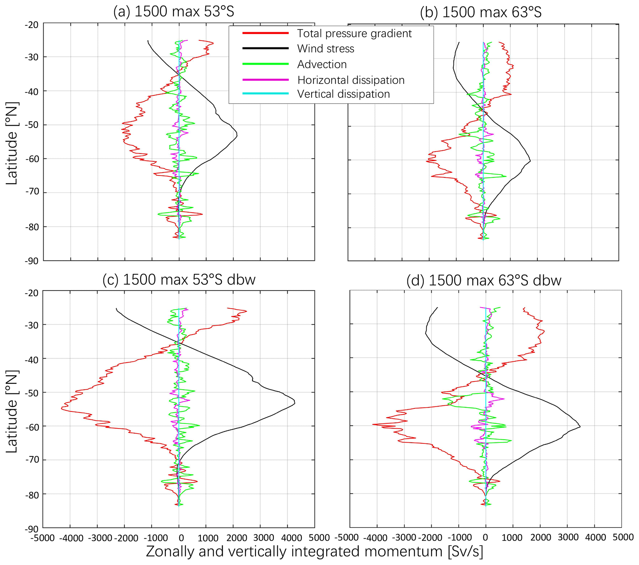
Figure A1The vertically and zonally integrated zonal momentum budget: total pressure gradient (total form stress) (red; Sv s−1), wind stress (black; Sv s−1), advection (green; Sv s−1), horizontal dissipation (magenta; Sv s−1) and vertical dissipation (light blue; Sv s−1) in the 1500_max_53∘ S (a), 1500_max_63∘ S (b), 1500_max_53∘ S_dbw (c) and 1500_max_63∘ S_dbw (d) cases.
In Masich et al. (2015)'s method, the topographic form stress signal is extracted from the total pressure field. Every ocean grid box adjacent to a bathymetric feature (for example, a seamount) and its pressure, Pt, is found at every model level. The pressure difference across each piece of bathymetry, calculated as the value between the ocean grid adjacent to the eastern face of the seamount and the ocean grid adjacent to the western face, is then found (Fig. B1a and Eq. B1):
The pressure gradient is then calculated as the pressure difference divided by the width of the bathymetric feature (see Fig. B1b and Eq. B2):
The vertical and zonal integral then gives the total topographic form stress signal, as shown in Fig. B1c and Eq. (B3):
In our simulations, the total topographic form stress and total pressure gradient are almost equal, as the values of blue and red curves in the Fig. B2 are almost coincident. This indicates the accuracy of the method of Masich et al. (2015) for estimating the total topographic form stress. The slight difference between calculations is mostly due to ambiguity over the pressure and depth of partial cells, as discussed below.
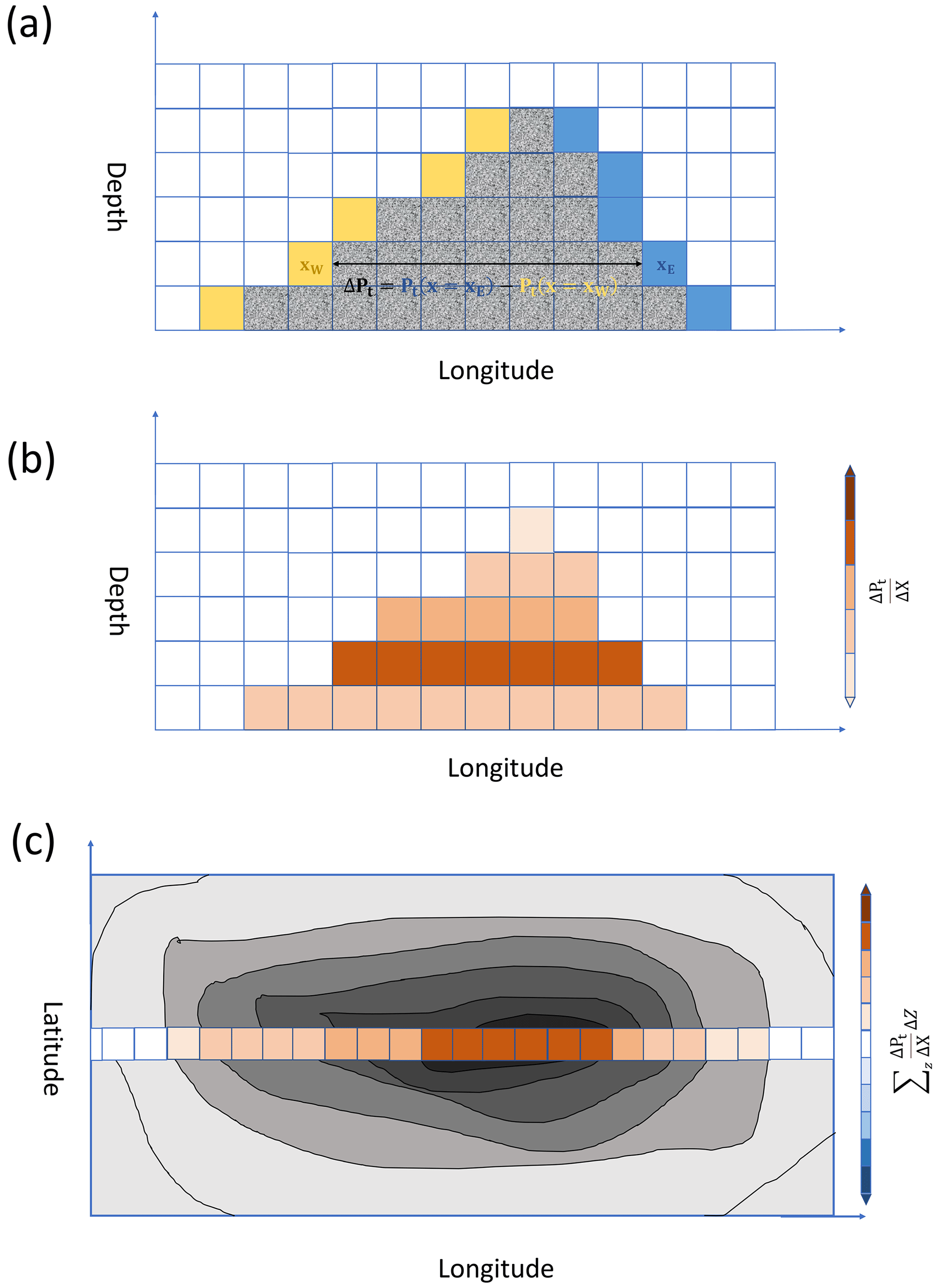
Figure B1Assume that there is a submerged seamount. Panel (a) shows a zonal slice of a seamount, where white cells indicate seawater and grey cells indicate landmasses. Grids in yellow are the grids adjacent to the western face of the seamount, and grids in blue are the grids adjacent to the eastern face of the seamount. In panel (b), the pressure difference is divided by the width of the seamount to give the , which is assigned to every grid of the seamount in each vertical level. Panel (c) shows the vertically integrated topographic form stress field across the seamount. This figure is adapted from Masich et al. (2015).
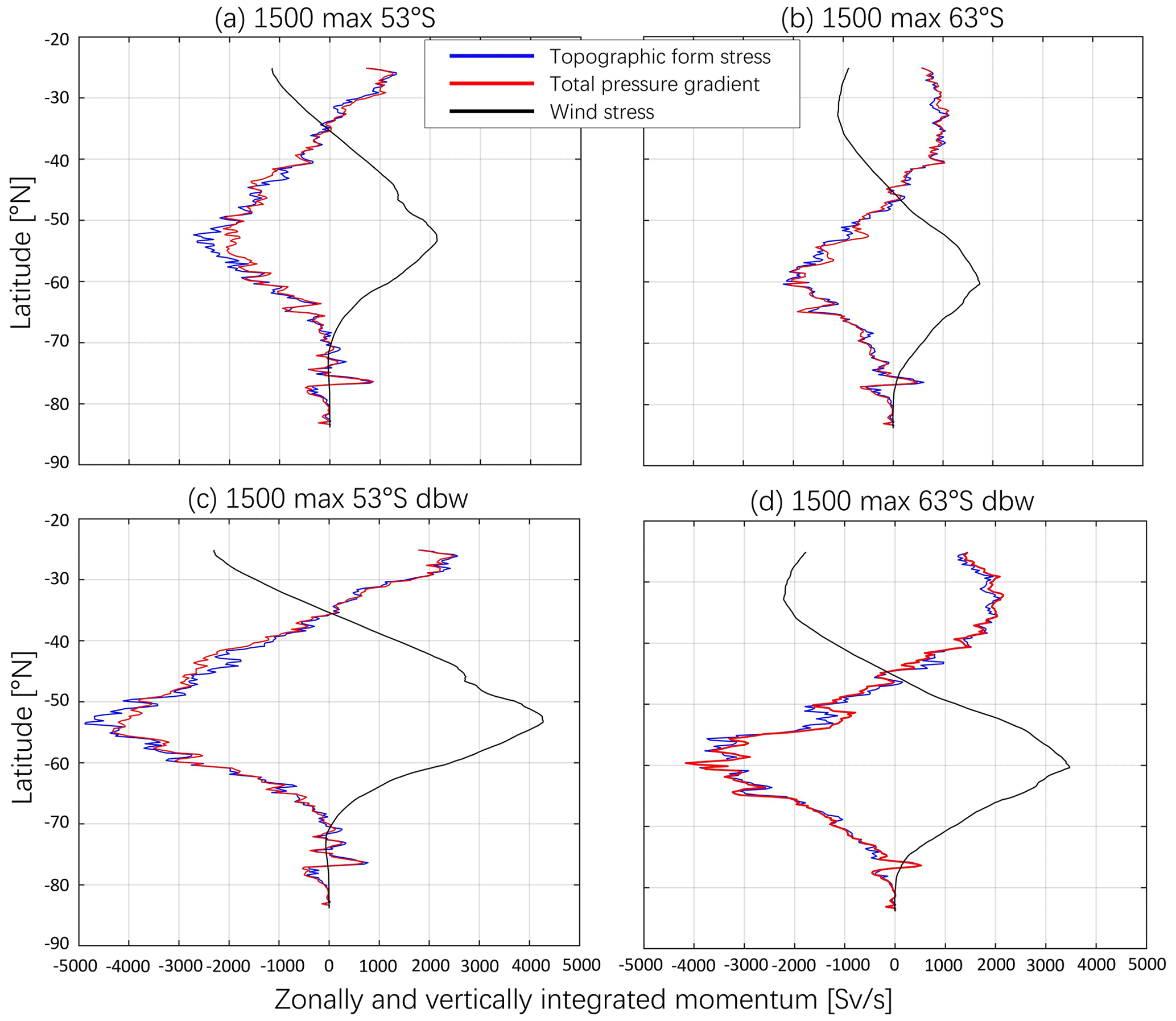
Figure B2The zonally and vertically integrated values of the momentum budget between wind stress (black; Sv s−1), total topographic form stress (blue; Sv s−1) and total pressure gradient (red; Sv s−1) in the 1500_max_53∘ S (a), 1500_max_63∘ S (b), 1500_max_53∘ S_dbw (c) and 1500_max_63∘ S_dbw (d) cases.
The method calculates the topographic form stress by taking the vertical and zonal integral of the pressure gradient (east minus west) between the fluid cell adjacent to the eastern face of the bathymetric features and the fluid cell adjacent to the western face (Masich et al., 2015).
The ocean model uses partial vertical cells for a better representation of the bathymetry. This means that a vertical fraction of each grid box is ocean, while the rest is land. To simplify the calculation, we treat all partial cells as land and select the adjacent ocean cell to extract the pressure of this face. This simplification results in an uncertainty in the calculation of the total topographic form stress due to the neglect of pressure changes in partial ocean cells. We provide an example to show how this uncertainty occurs and estimate its magnitude (Fig. C1).
We extract some partial cells with longitudes from −44.1250 to −42.8750∘ E, a latitude of 83.3750∘ S and a depth of 298.3048 m. At each grid box, Li is the fraction of the level thickness that is ocean, Pi is the pressure at the centre of the grid box and i is the index of the grid box. For this section of the domain in the 1500_max_53∘ S case, the extracted Li and Pi values are as follows: L1=0.3122, N m−2; L2=0.5305, N m−2; L3=0.7643, N m−2; L4=0.9608, N m−2; L5=1, N m−2.
Taking into account the pressure pushing on each partial cell wall, the pressure on the land (longitude from −44.1250 to −42.8750∘ E, latitude of 83.3750∘ S, depth of 298.3048 m), Pb, could be calculated as follows: N m−2.
In the method of estimating topographic form stress, we select the P5 as the fluid pressure on the land on the eastern side. The difference rate between Pb and P5 is %.
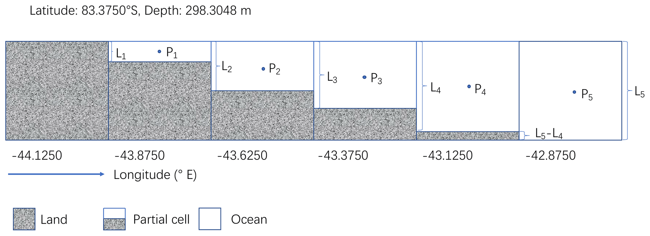
Figure C1Some model grid boxes that include land, partial cells, and ocean with longitudes from −44.1250 to −42.8750 ∘E, a latitude of 83.3750∘ S and a depth of 298.3048 m. Li is the fraction of the level thickness that is ocean, Pi is the pressure at the centre of the grid box and i is the index of the grid box.
Figure D1 shows the reconstructed bathymetry of Southern Ocean at 38 Ma and bathymetry of the 300 m and 1500 m TG; for the details of the late Eocene bathymetry reconstruction, refer to Sect. 2.2
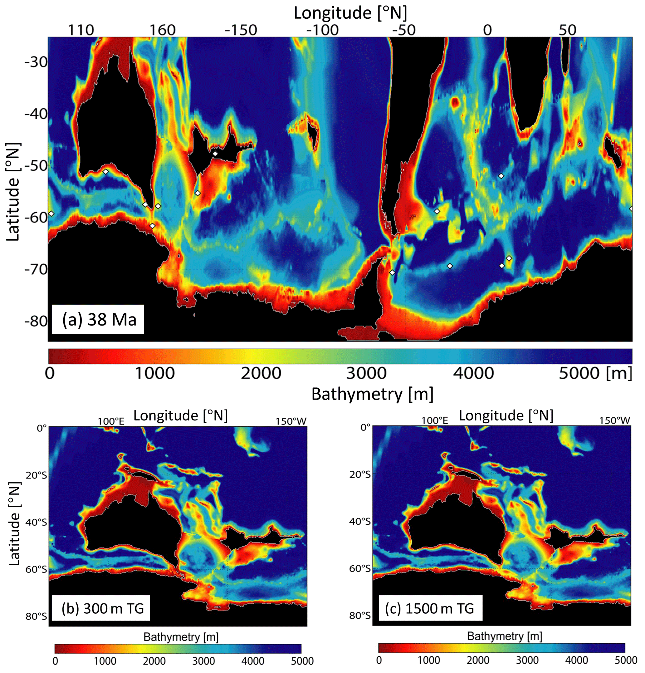
Figure D1(a) High-resolution (0.25∘) reconstructed bathymetry of the late Eocene (38 Ma) Southern Ocean. (b) Bathymetry of the 300 m TG. (c) Bathymetry of the 1500 m TG.
Figure E1 shows a time series of TG throughflow transport when TG is at 300 and 1500 m and wind stress is in four positions. The period is from model year 86 to 145. We can see that all transports are stable, implying a clear equilibrium in all simulations.
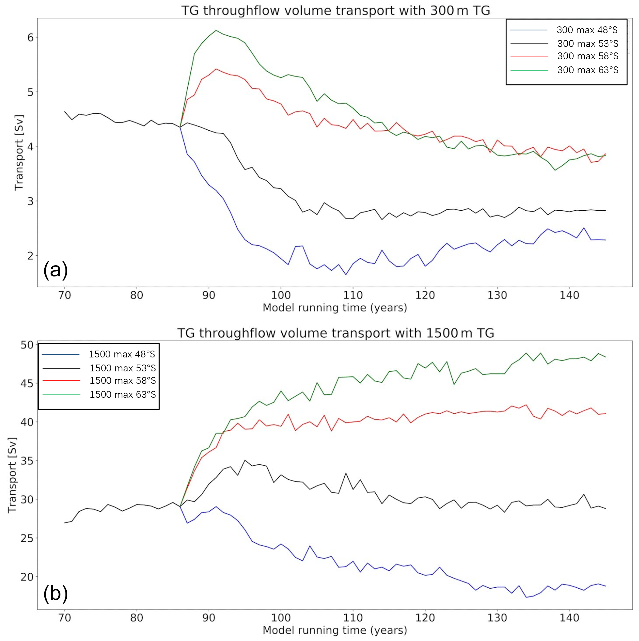
Figure E1(a) Time series of TG throughflow transport when TG is at 300 m. (b) Time series of TG throughflow transport when TG is at 1500 m. The period covered by both series is from model year 86 to 145.
The “bottom flow transport” (Tb) and “thermal wind transport” (Ttw) are given by the following equations:
Equations F1 and F2) refer to Eqs. (4) and (5) in Munday et al. (2015). However, there is a difference when calculating the zonal bottom flow velocity Ub. By looking at hydrographic sections of the local bathymetry and U velocity for the TG and DP, respectively, we select a model level (e.g. Fig. F1 model level 32), below which the current velocities have weak vertical and meridional gradients andabove which the velocities show strong horizontal and vertical gradients. Then we use a vertical average of zonal velocity below that model level as the Ub.
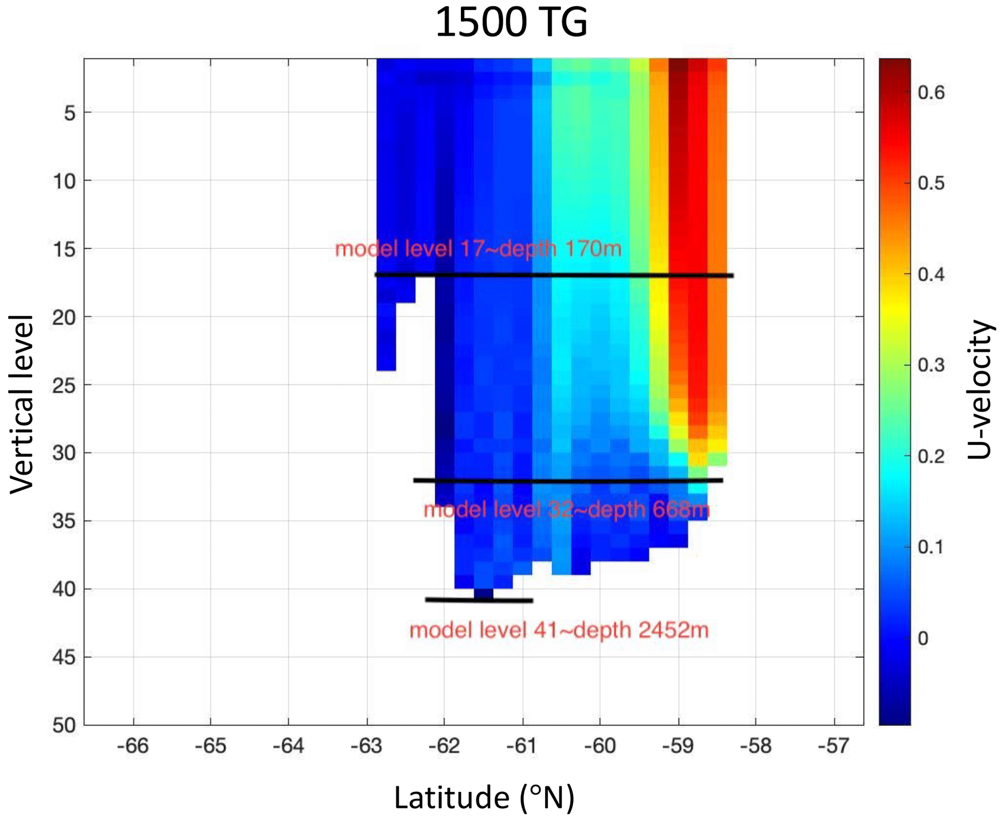
Figure F1Hydrographic sections of the zonal velocities through the 1500 m TG. The vertical level is the uneven model level. Black lines show some unique levels and the corresponding depths.
The model data can be downloaded from the Australian National Computational Infrastructure. An email can be sent to Qianjiang Xing (qianjiang.xing@utas.edu.au) for access.
The model configuration was established by AK, DM and JW. IS performed the spin-up simulation, and QX changed the wind stress and performed further simulations. QX analysed the results and finished the manuscript with supervision from AK, DM and JW. IS helped to plot Fig. 1 and gave a lot of suggestions for improving the manuscript. All authors reviewed the manuscript.
The contact author has declared that none of the authors has any competing interests.
Publisher's note: Copernicus Publications remains neutral with regard to jurisdictional claims in published maps and institutional affiliations.
We acknowledge the Australian National Computational Infrastructure Merit Allocation Scheme projects used for running the model simulations. We are grateful for discussions with Edward Doddridge about ocean modelling and with Xihan Zhang about estimating topographic form stress. We are grateful to Michiel Baatsen and the anonymous reviewer for their substantial and useful comments that improved the manuscript. We also thank to the editor Yannick Donnadieu for helpful guidance.
This work was funded by the Australian Research Council Discovery Project (DP180102280). Isabel Sauermilch is supported by the ARC Discovery Project (DP180102280) and ERC starting grant OceaNice (802835).
This paper was edited by Yannick Donnadieu and reviewed by Michiel Baatsen and one anonymous referee.
Baatsen, M., van Hinsbergen, D. J. J., von der Heydt, A. S., Dijkstra, H. A., Sluijs, A., Abels, H. A., and Bijl, P. K.: Reconstructing geographical boundary conditions for palaeoclimate modelling during the Cenozoic, Clim. Past, 12, 1635–1644, https://doi.org/10.5194/cp-12-1635-2016, 2016. a, b
Baatsen, M., von der Heydt, A., Kliphuis, M., Viebahn, J., and Dijkstra, H.: Multiple states in the late Eocene ocean circulation, Global Planet. Change, 163, 18–28, 2018. a
Baatsen, M., von der Heydt, A. S., Huber, M., Kliphuis, M. A., Bijl, P. K., Sluijs, A., and Dijkstra, H. A.: The middle to late Eocene greenhouse climate modelled using the CESM 1.0.5, Clim. Past, 16, 2573–2597, https://doi.org/10.5194/cp-16-2573-2020, 2020. a, b, c
Barker, P. and Thomas, E.: Origin, signature and palaeoclimatic influence of the Antarctic Circumpolar Current, Earth-Sci. Rev., 66, 143–162, 2004. a
Bijl, P. K., Bendle, J. A., Bohaty, S. M., Pross, J., Schouten, S., Tauxe, L., Stickley, C. E., McKay, R. M., Röhl, U., Olney, M., and Sluijs, A.: Eocene cooling linked to early flow across the Tasmanian Gateway, P. Natl. Acad. Sci. USA, 110, 9645–9650, 2013. a, b
Bryan, K.: Poleward heat transport by the ocean: observations and models, Annu. Rev. Earth Planet. Sci., 10, 15, 1982. a
Chidichimo, M. P., Donohue, K. A., Watts, D. R., and Tracey, K. L.: Baroclinic transport time series of the Antarctic Circumpolar Current measured in Drake Passage, J. Phys. Oceanogr., 44, 1829–1853, 2014. a
Daru, V. and Tenaud, C.: High order one-step monotonicity-preserving schemes for unsteady compressible flow calculations, J. Comput. Phys., 193, 563–594, 2004. a
Delworth, T. L., Rosati, A., Anderson, W., Adcroft, A. J., Balaji, V., Benson, R., Dixon, K., Griffies, S. M., Lee, H. C., Pacanowski, R. C., and Vecchi, G. A.: Simulated climate and climate change in the GFDL CM2.5 high-resolution coupled climate model, J. Climate, 25, 2755–2781, 2012. a, b
Donohue, K., Tracey, K., Watts, D., Chidichimo, M. P., and Chereskin, T.: Mean antarctic circumpolar current transport measured in drake passage, Geophys. Res. Lett., 43, 11–760, 2016. a
Gille, S. T.: The Southern Ocean momentum balance: Evidence for topographic effects from numerical model output and altimeter data, J. Phys. Oceanogr., 27, 2219–2232, 1997. a
Grezio, A., Wells, N., Ivchenko, V., and De Cuevas, B.: Dynamical budgets of the Antarctic Circumpolar Current using ocean general-circulation models, Q. J. Roy. Meteorol. Soc., 131, 833–860, 2005. a
Hallberg, R.: Using a resolution function to regulate parameterizations of oceanic mesoscale eddy effects, Ocean Model., 72, 92–103, 2013. a
Hallberg, R. and Gnanadesikan, A.: An exploration of the role of transient eddies in determining the transport of a zonally reentrant current, J. Phys. Oceanogr., 31, 3312–3330, 2001. a
Haney, R. L.: Surface thermal boundary condition for ocean circulation models, J. Phys. Oceanogr, 1, 241–248, 1971. a
Hill, D. J., Haywood, A. M., Valdes, P. J., Francis, J. E., Lunt, D. J., Wade, B. S., and Bowman, V. C.: Paleogeographic controls on the onset of the Antarctic circumpolar current, Geophys. Res. Lett., 40, 5199–5204, 2013. a, b, c, d
Hochmuth, K., Gohl, K., Leitchenkov, G., Sauermilch, I., Whittaker, J. M., Uenzelmann-Neben, G., Davy, B., and De Santis, L.: The evolving paleobathymetry of the circum-Antarctic Southern Ocean since 34 Ma: a key to understanding past cryosphere-ocean developments, Geochem. Geophy. Geosy., 21, e2020GC009122, https://doi.org/10.1029/2020GC009122, 2020. a, b, c
Huber, M. and Nof, D.: The ocean circulation in the southern hemisphere and its climatic impacts in the Eocene, Palaeogeogr. Palaeocl., 231, 9–28, 2006. a, b
Huber, M., Brinkhuis, H., Stickley, C. E., Döös, K., Sluijs, A., Warnaar, J., Schellenberg, S. A., and Williams, G. L.: Eocene circulation of the Southern Ocean: Was Antarctica kept warm by subtropical waters?, Paleoceanography, 19, PA4026, https://doi.org/10.1029/2004PA001014, 2004. a, b, c, d, e, f
Hutchinson, D. K., de Boer, A. M., Coxall, H. K., Caballero, R., Nilsson, J., and Baatsen, M.: Climate sensitivity and meridional overturning circulation in the late Eocene using GFDL CM2.1, Clim. Past, 14, 789–810, https://doi.org/10.5194/cp-14-789-2018, 2018. a, b, c, d, e
Johnson, G. C. and Bryden, H. L.: On the size of the Antarctic Circumpolar Current, Deep-Sea Res. Pt. A, 36, 39–53, 1989. a, b
Johnson, J. and Hill, R.: A three-dimensional model of the Southern Ocean with bottom topography, in: Deep Sea Research and Oceanographic Abstracts, vol. 22, Elsevier, 745–751, https://doi.org/10.1016/0011-7471(75)90079-0, 1975. a
Kennedy, A. T., Farnsworth, A., Lunt, D., Lear, C. H., and Markwick, P.: Atmospheric and oceanic impacts of Antarctic glaciation across the Eocene–Oligocene transition, Philos. T. Roy. Soc. A, 373, 20140419, https://doi.org/10.1098/rsta.2014.0419, 2015. a, b
Kennett, J. P.: Cenozoic evolution of Antarctic glaciation, the circum-Antarctic Ocean, and their impact on global paleoceanography, J. Geophys. Res., 82, 3843–3860, 1977. a, b, c, d
Koenig, Z., Provost, C., Ferrari, R., Sennéchael, N., and Rio, M.-H.: Volume transport of the Antarctic Circumpolar Current: Production and validation of a 20 year long time series obtained from in situ and satellite observations, J. Geophys. Res.-Oceans, 119, 5407–5433, https://doi.org/10.1002/2014JC009966, 2014. a
LaCasce, J. H.: The prevalence of oceanic surface modes, Geophys. Res. Lett., 44, 11097–11105., https://doi.org/10.1002/2017GL075430, 2017. a
Lacasce, J. H., Escartin, J., Chassignet, E. P., and Xu, X.: Jet instability over smooth, corrugated, and realistic bathymetry, J. Phys. Oceanogr., 49, 585–605, 2019. a
Large, W. G., McWilliams, J. C., and Doney, S. C.: Oceanic vertical mixing: A review and a model with a nonlocal boundary layer parameterization, Rev. Geophys., 32, 363–403, 1994. a
Livermore, R., Hillenbrand, C.-D., Meredith, M., and Eagles, G.: Drake Passage and Cenozoic climate: an open and shut case?, Geochem. Geophy. Geosy., 8, Q01005, https://doi.org/10.1029/2005GC001224, 2007. a
Lyle, M., Gibbs, S., Moore, T. C., and Rea, D. K.: Late Oligocene initiation of the Antarctic circumpolar current: evidence from the South Pacific, Geology, 35, 691–694, 2007. a
Marshall, D.: Topographic steering of the Antarctic circumpolar current, J. Phys. Oceanogr., 25, 1636–1650, 1995. a
Marshall, D. P., Ambaum, M. H., Maddison, J. R., Munday, D. R., and Novak, L.: Eddy saturation and frictional control of the Antarctic Circumpolar Current, Geophys. Res. Lett., 44, 286–292, 2017. a
Marshall, J., Adcroft, A., Hill, C., Perelman, L., and Heisey, C.: A finite-volume, incompressible Navier Stokes model for studies of the ocean on parallel computers, J. Geophys. Res.-Oceans, 102, 5753–5766, 1997a. a
Marshall, J., Hill, C., Perelman, L., and Adcroft, A.: Hydrostatic, quasi-hydrostatic, and nonhydrostatic ocean modeling, J. Geophys. Res.-Oceans, 102, 5733–5752, 1997b. a
Masich, J., Chereskin, T. K., and Mazloff, M. R.: Topographic form stress in the Southern Ocean State Estimate, J. Geophys. Res.-Oceans, 120, 7919–7933, 2015. a, b, c, d, e, f, g, h, i, j
Matthews, K. J., Maloney, K. T., Zahirovic, S., Williams, S. E., Seton, M., and Mueller, R. D.: Global plate boundary evolution and kinematics since the late Paleozoic, Global Planet. Change, 146, 226–250, 2016. a, b, c
Mazloff, M. R., Heimbach, P., and Wunsch, C.: An eddy-permitting Southern Ocean State Estimate, J. Phys. Oceanogr., 40, 880–899, https://doi.org/10.1175/2009JPO4236.1, 2010. a
Mecking, J., Drijfhout, S. S., Jackson, L. C., and Graham, T.: Stable AMOC off state in an eddy-permitting coupled climate model, Clim. Dynam., 47, 2455–2470, 2016. a
Megann, A.: Estimating the numerical diapycnal mixing in an eddy-permitting ocean model, Ocean Model., 121, 19–33, 2018. a
Meredith, M. P., Woodworth, P. L., Chereskin, T. K., Marshall, D. P., Allison, L. C., Bigg, G. R., Donohue, K., Heywood, K. J., Hughes, C. W., Hibbert, A., and Hogg, A. M.: Sustained monitoring of the Southern Ocean at Drake Passage: Past achievements and future priorities, Rev. Geophys., 49, RG4005, https://doi.org/10.1029/2010RG000348, 2011. a, b
Munday, D., Johnson, H., and Marshall, D.: The role of ocean gateways in the dynamics and sensitivity to wind stress of the early Antarctic Circumpolar Current, Paleoceanography, 30, 284–302, 2015. a, b, c, d, e, f, g, h, i, j
Munday, D. R., Johnson, H. L., and Marshall, D. P.: Eddy saturation of equilibrated circumpolar currents, J. Phys. Oceanogr., 43, 507–532, 2013. a, b
Munday, D. R., Zhai, X., Harle, J., Coward, A. C., and Nurser, A. G.: Relative vs. absolute wind stress in a circumpolar model of the Southern Ocean, Ocean Model., 168, 101891, https://doi.org/10.1016/j.ocemod.2021.101891, 2021. a
Munk, W. H.: On the wind-driven ocean circulation, J. Atmos. Sci., 7, 80–93, 1950. a
Munk, W. H. and Palmén, E.: Note on the dynamics of the antarctic circumpolar current 1, Tellus, 3, 53–55, 1951. a
Murphy, M. G. and Kennett, J. P.: Development of latitudinal thermal gradients during the Oligocene: Oxygen isotope evidence from the southwest Pacific, in: Initial Reports of the Deep Sea Drilling Project 90, US Govt. Printing Office, Washington, 1347–1360, https://doi.org/10.2973/dsdp.proc.90.140.1986, 1986. a
Olbers, D.: Comments on “On the obscurantist physics of `form drag' in theorizing about the Circumpolar Current”, J. Phys. Oceanogr., 28, 1647–1654, 1998. a
Parsons, B. and Sclater, J. G.: An analysis of the variation of ocean floor bathymetry and heat flow with age, J. Geophys. Res., 82, 803–827, 1977. a
Royer, J.-Y. and Rollet, N.: Plate-tectonic setting of the Tasmanian region, Aust. J. Earth Sci., 44, 543–560, 1997. a
Sauermilch, I., Whittaker, J. M., Klocker, A., Munday, D. R., Hochmuth, K., Bijl, P. K., and LaCasce, J. H.: Gateway-driven weakening of ocean gyres leads to Southern Ocean cooling, Nat. Commun., 12, 1–8, 2021. a, b, c, d, e, f, g, h, i, j, k, l, m, n, o, p, q, r, s, t, u, v, w, x, y
Scher, H. D. and Martin, E. E.: Timing and climatic consequences of the opening of Drake Passage, Science, 312, 428–430, 2006. a
Scher, H. D., Whittaker, J. M., Williams, S. E., Latimer, J. C., Kordesch, W. E., and Delaney, M. L.: Onset of Antarctic Circumpolar Current 30 million years ago as Tasmanian Gateway aligned with westerlies, Nature, 523, 580–583, 2015. a, b, c, d, e, f, g, h
Sijp, W. P. and England, M. H.: Effect of the Drake Passage throughflow on global climate, J. Phys. Oceanogr., 34, 1254–1266, 2004. a, b
Sijp, W. P., England, M. H., and Huber, M.: Effect of the deepening of the Tasman Gateway on the global ocean, Paleoceanography, 26, PA4207, https://doi.org/10.1029/2011PA002143, 2011. a, b, c
Spence, P., Saenko, O. A., Dufour, C. O., Le Sommer, J., and England, M. H.: Mechanisms maintaining Southern Ocean meridional heat transport under projected wind forcing, J. Phys. Oceanogr., 42, 1923–1931, 2012. a
Steckler, M. and Watts, A.: Subsidence of the Atlantic-type continental margin off New York, Earth Planet. Sc. Lett., 41, 1–13, 1978. a
Stickley, C. E., Brinkhuis, H., Schellenberg, S. A., Sluijs, A., Röhl, U., Fuller, M., Grauert, M., Huber, M., Warnaar, J., and Williams, G. L.: Timing and nature of the deepening of the Tasmanian Gateway, Paleoceanography, 19, PA4026, https://doi.org/10.1029/2004PA001022, 2004. a, b, c, d
Stommel, H.: The westward intensification of wind-driven ocean currents, Eos Trans. Am. Geophys. Union, 29, 202–206, 1948. a
Straub, D. N.: On the transport and angular momentum balance of channel models of the Antarctic Circumpolar Current, J. Phys. Oceanogr., 23, 776–782, 1993. a
Tansley, C. E. and Marshall, D. P.: On the dynamics of wind-driven circumpolar currents, J. Phys. Oceanogr., 31, 3258–3273, 2001. a
Toggweiler, J. and Bjornsson, H.: Drake Passage and palaeoclimate, J. Quatern. Sci., 15, 319–328, 2000. a
Torsvik, T. H., Müller, R. D., Van der Voo, R., Steinberger, B., and Gaina, C.: Global plate motion frames: toward a unified model, Rev. Geophys., 46, RG3004, https://doi.org/10.1029/2007RG000227, 2008. a
van de Lagemaat, S. H., Swart, M. L., Vaes, B., Kosters, M. E., Boschman, L. M., Burton-Johnson, A., Bijl, P. K., Spakman, W., and Van Hinsbergen, D. J.: Subduction initiation in the Scotia Sea region and opening of the Drake Passage: When and why?, Earth-Sci. Rev., 215, 103551, https://doi.org/10.1016/j.earscirev.2021.103551, 2021. a
van Hinsbergen, D. J., De Groot, L. V., van Schaik, S. J., Spakman, W., Bijl, P. K., Sluijs, A., Langereis, C. G., and Brinkhuis, H.: A paleolatitude calculator for paleoclimate studies, PloS One, 10, e0126946, https://doi.org/10.1371/journal.pone.0126946, 2015. a, b, c
Viebahn, J. P., von der Heydt, A. S., Le Bars, D., and Dijkstra, H. A.: Effects of Drake Passage on a strongly eddying global ocean, Paleoceanography, 31, 564–581, 2016. a
Ward, M. L. and Hogg, A. M.: Establishment of momentum balance by form stress in a wind-driven channel, Ocean Model., 40, 133–146, 2011. a, b, c
Weatherall, P., Marks, K. M., Jakobsson, M., Schmitt, T., Tani, S., Arndt, J. E., Rovere, M., Chayes, D., Ferrini, V., and Wigley, R.: A new digital bathymetric model of the world's oceans, Earth Space Sci., 2, 331–345, 2015. a
Zhai, X. and Munday, D. R.: Sensitivity of Southern Ocean overturning to wind stress changes: Role of surface restoring time scales, Ocean Model., 84, 12–25, 2014. a, b
- Abstract
- Introduction
- Methods
- Results
- Discussion
- Conclusions
- Appendix A: Zonal momentum balance
- Appendix B: Derivation of the topographic form stress
- Appendix C: Uncertainty when calculating topographic form stress
- Appendix D: The reconstructed paleo-bathymetry used in the simulation
- Appendix E: Time series of TG throughflow transport
- Appendix F: Derivation of the bottom flow transport and thermal wind transport
- Data availability
- Author contributions
- Competing interests
- Disclaimer
- Acknowledgements
- Financial support
- Review statement
- References