the Creative Commons Attribution 4.0 License.
the Creative Commons Attribution 4.0 License.
 | 20 Dec 2022
Evaluation of statistical climate reconstruction methods based on pseudoproxy experiments using linear and machine-learning methods
Zeguo Zhang
Sebastian Wagner
Marlene Klockmann
Eduardo Zorita
Three different climate field reconstruction (CFR) methods are employed to reconstruct spatially resolved North Atlantic–European (NAE) and Northern Hemisphere (NH) summer temperatures over the past millennium from proxy records. These are tested in the framework of pseudoproxy experiments derived from two climate simulations with comprehensive Earth system models. Two of these methods are traditional multivariate linear methods (principal component regression, PCR, and canonical correlation analysis, CCA), whereas the third method (bidirectional long short-term memory neural network, Bi-LSTM) belongs to the category of machine-learning methods. In contrast to PCR and CCA, Bi-LSTM does not need to assume a linear and temporally stable relationship between the underlying proxy network and the target climate field. In addition, Bi-LSTM naturally incorporates information about the serial correlation of the time series. Our working hypothesis is that the Bi-LSTM method will achieve a better reconstruction of the amplitude of past temperature variability. In all tests, the calibration period was set to the observational period, while the validation period was set to the pre-industrial centuries. All three methods tested herein achieve reasonable reconstruction performance on both spatial and temporal scales, with the exception of an overestimation of the interannual variance by PCR, which may be due to overfitting resulting from the rather short length of the calibration period and the large number of predictors. Generally, the reconstruction skill is higher in regions with denser proxy coverage, but it is also reasonably high in proxy-free areas due to climate teleconnections. All three CFR methodologies generally tend to more strongly underestimate the variability of spatially averaged temperature indices as more noise is introduced into the pseudoproxies. The Bi-LSTM method tested in our experiments using a limited calibration dataset shows relatively worse reconstruction skills compared to PCR and CCA, and therefore our working hypothesis that a more complex machine-learning method would provide better reconstructions for temperature fields was not confirmed. In this particular application with pseudoproxies, the implied link between proxies and climate fields is probably close to linear. However, a certain degree of reconstruction performance achieved by the nonlinear LSTM method shows that skill can be achieved even when using small samples with limited datasets, which indicates that Bi-LSTM can be a tool for exploring the suitability of nonlinear CFRs, especially in small data regimes.
- Article
(14692 KB) - Full-text XML
- BibTeX
- EndNote


The reconstruction of past climates helps to better understand past climate variability and pose the projected future climate evolution against the backdrop of natural climate variability (Mann and Jones, 2003; Jones and Mann, 2004; Jones et al., 2009; Frank et al., 2010; Schmidt, 2010; Christiansen and Ljungqvist, 2012, 2017; Evans et al., 2014; Smerdon and Pollack, 2016). Paleoclimate reconstructions also provide us with a deeper perspective to better understand the effect of external forcing on climate (Hegerl et al., 2006, 2007; Schurer et al., 2013, 2014; Anchukaitis et al., 2012, 2017; Tejedor et al., 2021a, b). However, systematic observational and instrumental climate records are only available starting from the middle of the 19th century, which fails to capture the full spectrum of past climate variations. Consequently, our understanding of climate variations prior to 1850 is mainly based on indirect proxy records (such as tree rings and ice cores; Jones and Mann, 2004). The reconstruction of past climates based on proxy data requires the application of statistical methods to translate the information contained in the proxy records into climate variables such as temperature. These methods add an additional layer of statistical uncertainty and bias to the final reconstruction, in addition to the uncertainties originating in the sparse data coverage and in the presence of non-climatic variability in the proxy records. All these sources of error impact the quality of climate reconstructions. One way to estimate this impact is to test using reconstruction methods in the controlled conditions provided by climate simulations with state-of-the-art Earth system models. These models provide virtual climate trajectories, which are from the model's perspective physically consistent, despite possibly not being completely realistic. The skill of the statistical method and the impact of proxy network coverage and of the amount of climate signal present in the proxy records can thus be evaluated in that virtual reality of climate models once adequate synthetic proxy records are constructed. These tests are generally denoted as pseudoproxy experiments (PPEs; Smerdon, 2012; Gómez-Navarro et al., 2017).
Many scientific studies that employ pseudoproxies and real proxies have focused on global, hemispheric climate field, or climate index reconstructions (Mann and Rutherford, 2002; Mann et al., 2005; von Storch et al., 2004; Smerdon, 2012; Michel et al., 2020; Hernández et al., 2020). These studies have identified several deficiencies that are common to most climate reconstruction methods, such as a general tendency to “regress to the mean”, which results in an underestimation of the reconstructed climate variability. This underestimation becomes more evident when the available proxy information becomes of lower quality, diminishing the climate signal contained in the proxy records. In addition, sparser networks, and thus shrinking proxy network coverage, may lead to biased reconstructions (Wang et al., 2014; Evans et al., 2014; Amrhein et al., 2020; Po-Chedley et al., 2020). Thus, significant scope still remains for further developing and evaluating climate field reconstruction (CFR) methodologies and designing methods that are less prone to those common deficiencies (Christiansen and Ljungqvist, 2017).
In the present study, we test a nonlinear CFR method that belongs to the machine-learning family, a bidirectional long short-term neural network (Bi-LSTM), which has not, to our knowledge, been applied to CFR yet. We compare the performance of this method to two well-established classical multi-variate linear regression methods, principal component regression (PCR), and canonical correlation analysis (CCA). Traditional CFRs usually assume linear and temporally stable relationships between the local variables captured by the proxy network and the target climate field. Likewise, the spatial patterns of climate variability are considered stationary (Coats et al., 2013; Pyrina et al., 2017; Wang et al., 2014; Smerdon et al., 2016; Yun et al., 2021). However, links between climate fields can be nonlinear (Schneider et al., 2018; Dueben and Bauer, 2018; Huntingford et al., 2019; Nadiga, 2020). Nonlinear machine-learning-based CFR methods (for instance, artificial neural networks, ANN) could help capture underlying linear and nonlinear relationships between proxy records and the large-scale climate (Rasp and Lerch, 2018; Schneider et al., 2018; Rolnick et al., 2019; Huang et al., 2020; Nadiga, 2020; Chattopadhyay et al., 2020; Lindgren et al., 2021). Moreover, machine-learning methods do not necessarily rely on statistical methods to first obtain the principal spatial climate patterns, such as principal component analysis (PCA). The full inherent variability in the original dataset is sequentially and dynamically adjusted and captured with optimized hyper-parameters during the model training process (Goodfellow et al., 2016).
Within the family of machine-learning methods, recurrent neural networks (RNNs) and long short-term memory networks (LSTMs) are characterized by specifically incorporating the sequential structure of the predictors to estimate the predictand (Bengio et al., 1994). This property makes them promising methods to ameliorate the underestimation of variability that affects many other methods. Our assumption here is that the methods would be able to better capture episodes of larger deviations from the mean, especially those that stretch over several time steps. However, this assumption is not guaranteed to be realistic in practical situations and needs to be tested. The classical recurrent neural network and long short-term memory network can usually only receive and process information from prior forward inference steps. A variant of the LSTM network is the bidirectional (Bi)-LSTM. It handles information from both forward and backward temporal directions (Graves and Schmidhuber, 2005). It has been demonstrated that the Bi-LSTM model is capable of learning and capturing long-term dependencies from a sequential dataset (Hochreiter and Schmidhuber, 1997) and that it achieves better performance for some classification and prediction tasks (Su et al., 2021; Biswas and Sinha, 2021; Biswas et al., 2021). Since climate dynamics usually exhibit temporal dependencies, the Bi-LSTM method might learn these dependencies better, which could provide another advantage when capturing the time evolution of the reconstructed climate field.
Bi-LSTM combines two independent LSTMs, which allows the network to incorporate both backward and forward information for the sequential time series at every time step. Our working hypothesis is that a more sophisticated type of RNN could better replicate the past variability, perhaps even more so for extreme values. Thus, we would like to test whether this property of Bi-LSTM is useful for paleoclimate research in the future based on our experiments, especially by employing only a limited calibration and training dataset that could also be a challenge for training deep neural networks (Najafabadi et al., 2015).
This calibration period, which is usually chosen in the real reconstructions as the observational period (or the overlap period between observations and proxy records), can represent a challenge not only for a parameter-rich method such as Bi-LSTM but also for the usual linear methods. For instance, a global or hemispheric proxy network may span of the order of 100 sites, and a regional proxy network may span a few dozen sites. If the calibration period spans at most 150 independent time steps, a method like principal component regression, in which one principal component is predicted by the whole proxy network, is rather close to overfitting conditions, especially in a global or hemispheric cases. Canonical correlation analysis with a PCA pre-filtering would be much more robust to the potential overfitting if only a few leading PCs are retained in the pre-filtering step (see Sect. 2.2.). Here, we test the methods in our pseudoproxy experiments in the conditions that they are usually applied in real reconstructions, in which overfitting may be a real risk.
For the sake of completeness, we briefly mention here the relevance for our study of the reconstruction methods that combine the assimilation of information from proxy and from climate simulations (Steiger et al., 2014; Carrassi et al., 2018). The family of data-assimilation methods constrain or modify the spatially complete output of climate simulations conditional on the sparse locally available information provided by proxy records. Therefore, they are in principle not so strongly constrained by the assumption that the spatial covariance is stationary over time. Another advantage is that they provide an estimation of reconstruction uncertainties in a more straightforward way, especially those methods formally based on a Bayesian framework. On the other hand, the underlying data-assimilation equations do require the estimation of large cross-covariance matrices, e.g., based on Kalman filters, and this usually makes the application of some sort of subjective regularization of the error-covariance matrices necessary (Harlim, 2017; Janjić et al., 2018). They also might be computationally much more demanding than purely data-driven methods. Considering the replication of the amplitude of past variations, it depends on factors that are independent of the method itself, such as the variance generated by the climate model and also on the inherent uncertainties of the proxy data. Therefore, an underestimation or overestimation of reconstructed variance cannot be characterized as a systemic property of these methods. They have the very important advantage in that they combine all of the available information about past climate (simulations, forcings, proxy data) into a powerful tool.
These special characteristics make the comparison with purely data-driven methods more difficult and probably unfair, since data assimilation uses a much larger amount of information from climate simulations. In addition, this use of information from climate simulations compromises one of the main objectives of climate reconstructions, namely the validation of climate models in climate regimes outside the variations of the observational period. Therefore, the testing of purely data-driven reconstruction methods retains its relevance, despite the availability of more sophisticated data-assimilation methods.
In this evaluation of three climate reconstruction methods, we focus on the whole Northern Hemisphere temperature field and on the temperature field of the North Atlantic–European region. In the North Atlantic region, the most important mode of temperature variations at longer time series is the Atlantic multidecadal variability (AMV). The AMV is sometimes defined as the decadal variability of the North Atlantic sea-surface temperature (SST), whereas the term Atlantic multidecadal oscillation (AMO) is reserved for the decadal internal variations (excluding the externally forced variability). Here we focus on the total variability of the North Atlantic SST and define the index of the AMV as the decadal filtered surface temperature anomaly over the North Atlantic region (0–70∘ N, 95∘ W–30∘ E), excluding the Mediterranean and Hudson Bay, following Knight et al. (2006). It has been shown that AMV is related to many prominent features of regional or even hemispheric multidecadal climate variability, for example European and North American summer climate variability (Knight et al., 2006; Qasmi et al., 2017). In this context, we test the reconstruction skill for the spatially resolved summer temperature anomalies over the Northern Hemisphere (NH; 0–90∘ N, 180∘ W–180∘ E) and North Atlantic–European region (NAE; 0–88∘ N, 60∘ W–30∘ E), as well as for the spatially averaged AMV and NH summer temperature anomalies, calculated from the spatially resolved reconstructed fields. The reconstruction of mean temperature series could provide a general assessment of the skill for reconstructing extreme temperature phases (e.g., related to volcanic eruptions or changes in solar activity), which can serve as benchmarks to test the potential capability of different CFR methods regarding those anomalies.
2.1 Data
2.1.1 Proxy data locations
Regarding the networks of real proxies used so far, St. George and Esper (2019) reviewed contemporary studies of previous NH temperature reconstructions based on tree ring proxies (Mann et al., 1998, 2008, 2007, 2009a, b; Emile-Geay et al., 2017). St. George and Esper (2019) concluded that the present-day generation of tree-ring-proxy-based reconstructions exhibit high correlations with seasonal hemispheric summer temperatures and display relatively good skill in tracking year-to-year climatic variabilities and decadal fluctuations compared to former proxy networks, as found by Wilson et al. (2016) and Anchukaitis et al. (2017). Thus, we test NH summer temperature CFRs employing a pseudoproxy continental network that is the result of blending two networks: the PAGES 2k Consortium (Emile-Geay et al., 2017) multiproxy network and the climate–tree ring network of St. George (2014).
In the oceanic realm in the North Atlantic, additional marine proxy records based on mollusk shell bands (Pyrina et al., 2017) have also been used for climate reconstructions. These records, similar to the dendroclimatological records, are based on annual growth bands, are annually resolved, and usually represent surface or subsurface water temperature. Therefore, they are technically rather similar to dendroclimatological records. Compelling evidence has already been provided by earlier studies that Atlantic Ocean variability is an important driver of European summer climate variability (Jacobeit et al., 2003; Sutton and Hodson, 2005; Folland et al., 2009). Thus, we also employ an updated proxy network by combining the locations of marine proxies and tree ring proxies (Pyrina et al., 2017; Emile-Geay et al., 2017; Luterbacher et al., 2016) to test the NAE summer temperature reconstructions.
The pseudoproxies are constructed from the simulated grid cell summer mean temperature sampled from two climate model simulations over the past millennium (see following subsections). In this context, 11 real proxy locations in the North Atlantic–European region (Pyrina et al., 2017; Emile-Geay et al., 2017; Luterbacher et al., 2016) are selected for regional NAE (0–88∘ N, 60∘ W–30∘ E) PPEs, while 48 proxy locations across the Northern Hemisphere are chosen from the PAGES 2k network. The original Northern Hemisphere PAGES network was trimmed down by removing proxies that may show a combined temperature–moisture response and by selecting only one proxy among those deemed to be too closely located (and thus redundant from the climate model perspective). Specifically, the 48 dendrochronology locations are selected according to Fig. 4 of St. George (2014), which shows the correlation coefficient between the dendroclimatological proxy records and summer temperature. At most of the retained locations, the correlation between the dendroclimatological record and regional temperature is higher than 0.5.
2.1.2 Climate models
The choice of climate models to run pseudo-experiments will have an impact on the estimation of method skills (Smerdon et al., 2011, 2015; Parsons et al., 2021), since the spatial and temporal cross-correlations between climate variables are usually model dependent. Thus, it is advisable to use several “numerical laboratories” and employ several comprehensive Earth system models (ESMs) to evaluate reconstructions methods. Constructing PPEs based on different ESMs will highlight model-based impacts on the reconstructed magnitude and spatial patterns (Smerdon et al., 2011; Smerdon, 2012; Amrhein et al., 2020). Accordingly, in this study two different comprehensive ESMs are employed as a “surrogate” climate database for setting up PPEs: the Max-Planck-Institute Earth System Model model (MPI-ESM-P) and the Community Earth System Model (CESM).
One of the climate models utilized in our study is the Max-Planck-Institute Earth System Model (MPI-ESM-P) with a spatial horizontal resolution of about 1.9∘ in longitude and 1.9∘ in latitude. The simulation covers the period from 100 BCE to 2000 CE. The model MPI-ESM-P consists of the spectral atmospheric model ECHAM6 (Stevens et al., 2013), the ocean model MPI-OM (Jungclaus et al., 2013), the land model JSBACH (Reick et al., 2013), and the bio-geophysical model HAMOCC (Ilyina et al., 2013). The setup of our simulations corresponds to the MPI-ESM-P LR setup in the CMIP5 simulations suite. However, since the present simulation does not belong to the CMIP5 project, the forcings used in this simulation and additional technical details are shown in Appendix A.
The second climate model is the Community Earth System Model (CESM) Paleoclimate model from the National Center for Atmospheric Research (NCAR) (Otto-Bliesner et al., 2016) with a spatial resolution of 2.5∘ in longitude and 1.9∘ in latitude (https://www.cesm.ucar.edu/projects/community-projects/LME/, last access: 15 January 2022). The CESM simulation extends from 850 CE to 2006 CE using CMIP5 climate forcing reconstructions (Schmidt et al., 2011) and reconstructed forcing for the transient evolution of aerosols, solar irradiance, land use conditions, greenhouse gases, orbital parameters, and volcanic emissions. The atmosphere model employed in CESM is CAM5 (Hurrell et al., 2013), which is a significant advancement of CAM4 (Neale et al., 2013), whereas CCSM4 uses CAM4 as its atmospheric component. The CESM uses the same ocean, land, and sea ice models as CCSM4 (Hurrell et al., 2013). We use the last single-ensemble simulation (member 13) from the Last Millennium Ensemble (LME).
2.2 Methods
2.2.1 Construction of pseudoproxies
To test the statistical reconstruction methods in the virtual laboratories of climate model simulations, we need records that mimic the statistical properties of real proxy records. The most important properties are their correlation to the local temperature and their location in a proxy network. A third important characteristic is the network size and temporal coverage.
The usual method to produce pseudoproxy records in climate simulations is to sample the simulated temperature at the grid cell that contains the proxy location and contaminate the simulated temperature with added statistical noise so that the correlations between the original temperature and the contaminated temperature resembles the typical temperature–proxy correlations. The real correlation is on the order of 0.5 or above for good proxy records. This parameter can be modulated in the pseudoproxy record by the amount of noise added to the simulated temperature, and different proxy networks will help us to reveal how and to what extent degradations of reconstruction skill caused by the amount of non-climatic signals present in the pseudoproxies.
Ideal pseudoproxies contain only the temperature signal subsampled from the climate model. We then perturb the ideal pseudoproxies with Gaussian white noise and also with red noise for a more realistic noise contamination experiment. We generate two types of pseudoproxies by adding Gaussian white noise and red noise (refer to Pyrina et al., 2017) to the subsampled summer temperature time series at the tree-ring-proxy-based locations.
The noise level can be defined using various criteria including signal to noise ratio (SNR), variance of noise (NVAR), and percent of noise by variance (PNV) (Smerdon, 2012; Wang et al., 2014). We employ the PNV here to define the noise level convention. The PNV expresses the ratio between the added noise variance and the total variance of resulting the pseudoproxy time series. Without loss of generalization we assume that the ideal proxy has unit variance, and thus
Red noise for a specific PNV could be defined by
where Redt represents the red noise time series, α1 indicates the damping coefficient, here in our study it is equal to 0.4 (Larsen and MacDonald, 1995; Büntgen et al., 2010; Pyrina et al., 2017), and Whitet is a random white noise time series.
Although individual real proxies contain different amounts of noise (non-climatic variability), here we assume a uniform level of noise throughout the whole pseudoproxy network. In addition, real proxy records contain temporal gaps, and not all records span the same period. For the sake of simplicity, we assume in our pseudoproxies network that the data have no temporal gaps and that all records cover the whole period of the simulations.
The dataset employed here for constructing the according PPEs database is split into a calibration period that spans 1900–1999 CE, and a validation period that spans 850–1899 CE. This calibration period would represent the typical period of calibration of real proxy records. All the validation statistics of the CFR results are derived against the reconstruction period of 850–1899 CE.
2.2.2 Principal component regression
Principal component analysis is employed to construct a few new variables that are a linear combination of the components of the original climate field and that ideally describe a large part of the total variability. The linear combinations that define the new variables are the eigenvectors of the cross-covariance matrix of the field. Associated with each variable (eigenvector), a principal component time series (scores) describes its temporal variation. In the PCR, the predictands are those scores identified by PCA of the climate field (Hotelling, 1957; Luterbacher et al., 2004; Pyrina et al., 2017). This results in a reduction of dimensionality without losing too much information and reduces the risk of over-fitting. In the present study, the retained PCs capture at least 90 % of the cumulative temporal variance of climate field. After selecting the empirical orthogonal functions (EOFs) and principal components (PCs) based on the calibration dataset and establishing the desired linear regression relationships between the PCs and the proxy dataset (predictors), the PCs in the validation period are reconstructed using the estimated regression coefficients. The full climate field is then reconstructed by the linear combination of the reconstructed PCs and their corresponding EOFs. A given climate field xt at time step t can be decomposed as follows:
where m is the grid index of the field, t is the time index, and k denotes the total numbers of retained PCs.
The linear relationship between proxies and targeted climate field is established by the regression equation:
where the index m runs over the proxies, j denotes the total numbers of proxies, ω is the linear function coefficient, and ε denotes a residual term. The residual could be an unobserved random variable that adds noise to the linear relationship between the dependent variable (PC) and the targeted regressors (proxy or pseudoproxy) and includes all effects on the targeted regressors not related to the dependent variable (Christiansen, 2011).
The ω parameters are estimated by ordinary least squares. Here, it is assumed that climate-sensitive proxies are linearly related with the climate PCs. Based on Eq. (5) using the PCR method, the PCs during the validation interval will be reconstructed assuming that the linear coefficients derived in Eq. (5) are constant in time:
The final reconstructed field will be derived by the linear combination of the reconstructed with the EOFs derived from the calibration dataset, thereby assuming that the EOF patterns remain constant in time (Gómez-Navarro et al., 2017; Pyrina et al., 2017).
2.2.3 Canonical correlation analysis
Canonical correlation analysis (CCA) is also an eigenvector method. Similarly to PCA, CCA decomposes the variance of the fields as a linear combination of spatial patterns and their corresponding amplitude time series. In contrast to PCA, where the target is to maximize the explained variance with a few new variables, CCA constructs pairs of predictor–predictand variables that maximize the temporal correlation of the corresponding amplitude time series. The pairs of variables are identified by solving an eigenvalue problem that requires the calculation of the inverse of the covariance matrices of each field. These matrices can be pseudo-degenerate (one eigenvalue much smaller than the largest eigenvalue), and therefore the calculation of their inverse is, without regularization, numerically unstable. This regularization can be introduced by first projecting the original fields onto their leading EOFs (Widmann, 2005; Pyrina et al., 2017). This also reduces the number of degrees of freedom – thus hindering overfitting – and eliminate potential noise variance. After the dimensional transformation, a small number of pairs of patterns with high temporal correlation will be retained. In the present study, the number of retained PCs capture at least 90 % cumulative variance of predictand climate field. Then these retained PC time series will be used as input variables of CCA to calculate the canonical correlation patterns (CCPs) and canonical coefficients (CCs) time series for both the proxy and temperature field. The reconstructed climate field can be calculated by a linear combination of the CCPs with CCs for each time step t.
Proxy denotes the reconstructed proxy field, and l is the number of CCA pairs. The correlation between each pair CC (proxy, field) is the canonical correlation, which is the square root of the CCA eigenvalues. Therefore, once each CCproxy(t) is calculated from the proxy data through the validation period, the corresponding CCfield(t) can be easily estimated as proportional to CCproxy(t), since the correlation between the different is zero. The final reconstruction of the target climate field will be derived by a linear combination of CCPfield(t) and CCfield(t), assuming again that the dominant canonical correlation patterns of climate variability are stationary in time.
The CCA method maximizes the correlation that can be attained with a linear change of variables, i.e., with a linear combination of the grid cell series in each of the two fields. In the following, admittedly artificial, example, the resulting canonical correlation can be very high, and yet the reconstruction skill in general can remain low. If pair of grid cells, one each from the two fields, are very highly correlated to each other (and assuming here no PCA pre-filtering), CCA will pick those two cells as the first CCA pair (i.e., a pattern in each field with very high loadings only on those cells). The rest of the cells will not contribute to the CCA pattern. The reconstruction skill will therefore generally be very low in all those cells despite the canonical correlation being very high. In general, the reconstruction skill will be a monotonic function of the canonical correlation coefficient and the variance explained by the canonical predictand pattern. If the latter is low, the reconstruction skill will be low in large areas of the predictand field, even when the canonical correlation is possibly high.
2.2.4 Bidirectional long short-term memory neural network
As a nonlinear machine-learning method, here we test a bidirectional long short-term memory neural network (Bi-LSTM). The LSTM networks, in contrast to the more traditional neural networks, also capture the information of the serial co-variability present in the data, and therefore they are suitable to tackle data with a temporal structure. These methods are usually applied to the analysis of sequential data, such as speech and time series. The rationale of using these types of networks for climate reconstructions is the hypothesis that a better representation of the serial correlation could ameliorate the aforementioned underestimation of the past climate variations by most data-driven methods (“regression to the mean”, Smerdon, 2012).
The structure of LSTM network is more complex than the structure of a traditional neural network. The LSTM estimates a hidden variable h(t) that encapsulates the state of the system at time t. The computation of the new system state at time t+1, h(t+1), depends on the value of the predictors at t+1 but also on the value of the hidden state at time t, h(t). The training of the LSTM can be accomplished sequentially by assimilating the information present in the training data from time steps in the past of the present time step. In some loose sense, a LSTM network would be the machine-learning equivalent of a linear auto-regressive process.
A Bi-LSTM network, the training of the network is accomplished by feeding it with sequential data iteratively, both forwards towards the future and backwards towards the past. Both forward and backward assimilations are processed by two separated LSTM neural layers, which are connected to the same output layer. Figure 1 illustrates the bidirectional structure of the Bi-LSTM network. Given a set of predictor–predictand variables (Xt, Yt), our goal is to train a nonlinear function:
where is as close as possible to Yt. The similarity between and Yt is defined by a cost function. The structure of this complex nonlinear function F is defined as follows:
where Wf, Wi, WA, and Wo represent several weight matrices and Bf, Bi, BA, and Bo represent different bias matrices. σ is the gate activation function. Here we utilize the rectified linear unit function (ReLU; Ramachandran et al., 2017).

At time step t−1, the hidden state of LSTM cell's hidden layer is preserved as ht−1, and this vector is combined with the vector of current input variables Xt to obtain the state of the forget gate, ft (Eq. 9) and the input gate it (Eq. 10) and the state of memory cell At (Eq. 11). This memory cell state At is linearly combined with the previous state of the cell output Ct−1 to update the value of its state. The weights of these linear combinations are the states of the forget gate ft and of the input gate it (Eq. 12). The state of the output gate ot is calculated from the previous hidden state and the current input variables (Eq. 13). This output is used to compute the updated hidden state ht using the state of the cell output Ct (Eq. 14) (Huang et al., 2020; Chattopadhyay et al., 2020).
In the present application to climate reconstructions, we have a set of input pseudoproxy data and an output target temperature time series ,…, yt−1]. The forward LSTM hidden state sequence (note the arrow direction) is calculated employing input information in a positive direction from time t−n to time t−1 iteratively, and for backward LSTM cell the hidden state sequence is computed using the input within a reverse direction from time t−1 to time t−n iteratively. The final outputs from the forward and backward LSTM cells are calculated utilizing the calculation equation (Cui et al., 2018; Jahangir et al., 2020):
where concat is the function used to concatenate the two output sequences and (Cui et al., 2018; Jahangir et al., 2020).
During the training process, the calibration dataset is fed into the LSTM cell, and it will map the potential latent relationships (both linear and nonlinear) between input and output variables by updating its weight and threshold matrices. The objective cost function for Bi-LSTM to be minimized during training is the Huber loss that expresses the mismatch between the reconstructed climate field and the “real” climate field from model simulations. We minimize the loss with gradient descent (Goodfellow et al., 2016). Huber loss has a key advantage of being less sensitive to outlier values:
where f denotes the neural network and the brackets denote the Euclidean norm. The Huber loss function changes from a quadratic to linear when δ (a positive real number) varies from small to big (Meyer, 2020). Huber loss will approach L2 loss when δ tends to be 0 and approach L1 when δ tends to be positive infinity; here we test its value and finally set δ 1.35. L2 is the square root of the sum of squared deviations, and L1 is the sum of absolute deviations.
The main mechanism of LSTM is that the LSTM block manages to develop a regulated information flow by controlling which proportion of information from the past should be “remembered” or should be “forgotten” as time advances. By controlling the regulation of the information flow, LSTM will manage to learn and preserve temporal characteristics and dependencies of the specific time series.
A neural network is generally composed of one input layer, several hidden layers, and one output layer. Many hyper-parameters in the neural network usually need to be initialized and tuned for obtaining reasonable results within specific tasks, for instance, activation functions in each layer, objective functions for minimizing the loss of the network model, and learning rates for controlling the convergence speed of the network model (Goodfellow et al., 2016). In our specific CFR experiments, we have explored a range of Bi-LSTM architectures, including different network depths, introducing dropout layers, using different learning rates, and employing different loss functions to provide a more comprehensive evaluation of the Bi-LSTM performance and effectiveness (these tests are shown in Appendix B). These hyper-parameters within Bi-LSTM are finally selected and employed based on our experimental tests (Knerr et al., 1990; Kingma and Ba, 2014; Yu et al., 2019).
We evaluate the reconstruction skill of the different methods based on the Pearson correlation coefficient (cc) between each target series and the corresponding reconstructed series and their standard deviation ratio (SD ratio, ). All of the evaluation metrics are calculated in the validation period from 850 to 1899 CE. High values of derived cc indicate better temporal covariance between the target and reconstructed results, while a high SD ratio denotes that more variance is preserved in the reconstructions.
3.1 North Atlantic–European CFRs
Figure 2 illustrates the CFR results for the North Atlantic–European region employing the 11 ideal noise-free pseudoproxies based on the three CFR methodologies and the two climate model simulations. When comparing the reconstruction skills across these three CFR methods derived with the same climate model (for example, MPI and CESM), the spatial cc patterns calculated between targets and derived reconstructions among three CFR methods generally exhibit similarities. This indicates that all three CFR methods show generally reasonable spatial reconstruction skills (mean cc values over the entire NAE are bigger than 0.4). In addition, cc maps in Fig. 2 show higher values over regions with a denser pseudoproxy network. This confirms the well-documented tendency among different multivariate linear-based regression methods for better reconstruction skill in the sub-regions with denser pseudoproxy sampling than in regions with sparser networks (Smerdon et al., 2010, 2011; Steiger et al., 2014; Evans et al., 2014; Wang et al., 2014). The cc pattern of the nonlinear method Bi-LSTM is very similar to that of the linear methods, even though the structure of the statistical models is very different. This shows that the nonlinear method employed herein has as similar tendency to linear models for obtaining better reconstruction skill over regions with denser proxy sampling.
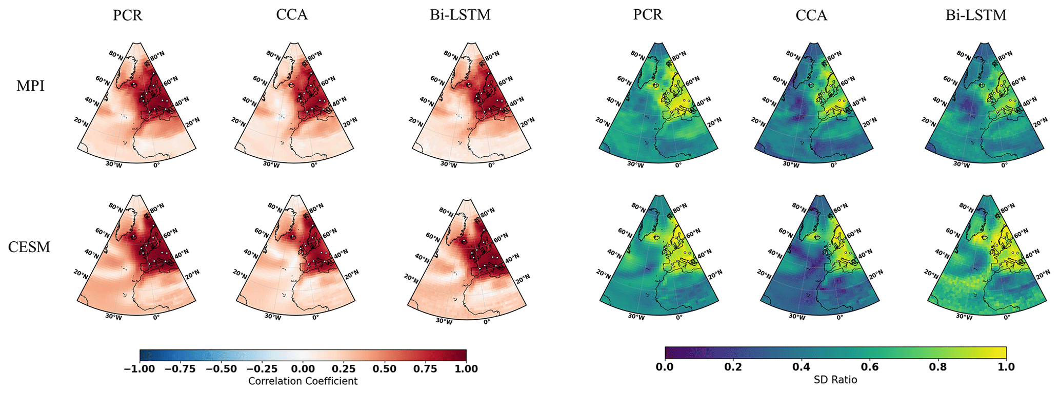
Figure 2NAE reconstruction results of CFR methods (including PCR, CCA, and Bi-LTSM) using MPI and CESM numerical simulations as the target temperature field. All of the CFR methods employ the same proxy network with a full set of 11 ideal pseudoproxies that span the same reconstruction period from 850 to 1899 CE. The employed pseudoproxy geolocations are shown as white circles in all panels. CC is correlation coefficient, and SD represents standard deviation.
The picture that emerges from the SD ratio is also very similar for the three methods (Fig. 2). In the regions with a high pseudoproxy density, the SD ratio is high, but outside of the densely sampled areas, all three CFR methods experience a similar degree of interannual variance underestimation. Appendix C displays the ratio of SD after applying a 30-year filter to the reconstructions and the target fields. The underestimation of variance is larger at these timescales, but the overall conclusion for all three methods remains.
Gaussian white and red noise is constructed and added to the ideal temperature signal of the 11 pseudoproxies subsampled from the MPI and CESM models. The corresponding spatial cc and SD ratio patterns are displayed in Figs. 3 and 4, respectively. Compared to reconstructions with ideal pseudoproxies (Fig. 2), a strong degradation of reconstruction skill among all CFR methods occurs over the entire NAE. The reduction in skill is especially profound in the regions where the pseudoproxy network is denser. Weak reconstruction skill exists over regions where proxies are available and within their proximity. These noise contamination results (shown in Figs. 3 and 4) again demonstrate that the nonlinear method exhibits CFR similarities to the linear methods, whereas Bi-LSTM shows relatively worse reconstruction skill, showing a variance underestimation compared to the other two methods using CESM-based PPEs (referring to the spatial SD ratio in Fig. 4).
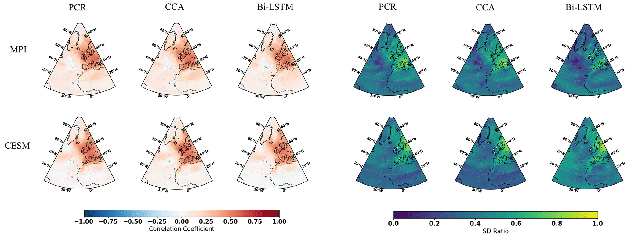
Figure 3The same as Fig. 2 but for employing the full 11-pseudoproxy network with white noise contamination.
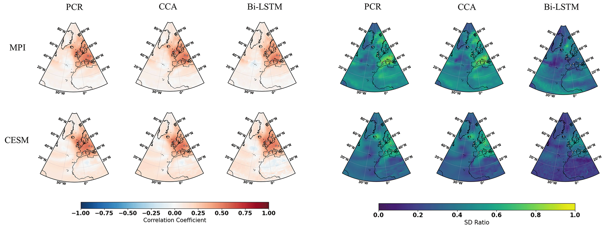
Figure 4The same as Fig. 2 but for employing the full 11-pseudoproxy network with red noise contamination.
The ratio of reconstructed to target variance after 30-year low-pass filtering is also larger than for the interannual variance, but otherwise the patterns share the same properties with the ratios of interannual SD (not shown for the sake of brevity).
In general, all three CFR methods exhibit similar reconstruction performance. Specifically, better skills over regions where denser pseudoproxies exist indicate that the spatial covariance patterns learned from the training data (in the 20th century) are stationary enough to represent the covariance during the reconstruction period over the NAE domain. It also shows that teleconnection patterns are to some degree localized and do not share a considerable amount of covariance outside of the sampled regions.
3.2 Northern Hemisphere CFRs
NH summer temperature anomaly reconstructions based on PPEs using three CFR methodologies and the three climate models are displayed in Figs. 5–7.
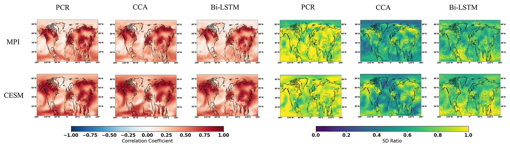
Figure 5NH reconstruction results of CFR methods (including PCR, CCA, and Bi-LSTM) using MPI and CESM numerical simulation as target temperature field. All of the CFR methods employ the same proxy network with the full set of 48 ideal pseudoproxies that span the same reconstruction period from 850 to 1899 CE. The employed pseudoproxies geolocations based on tree ring width (TRW) are shown as white circles in all panels. CC is correlation coefficient, and SD represents standard deviation.
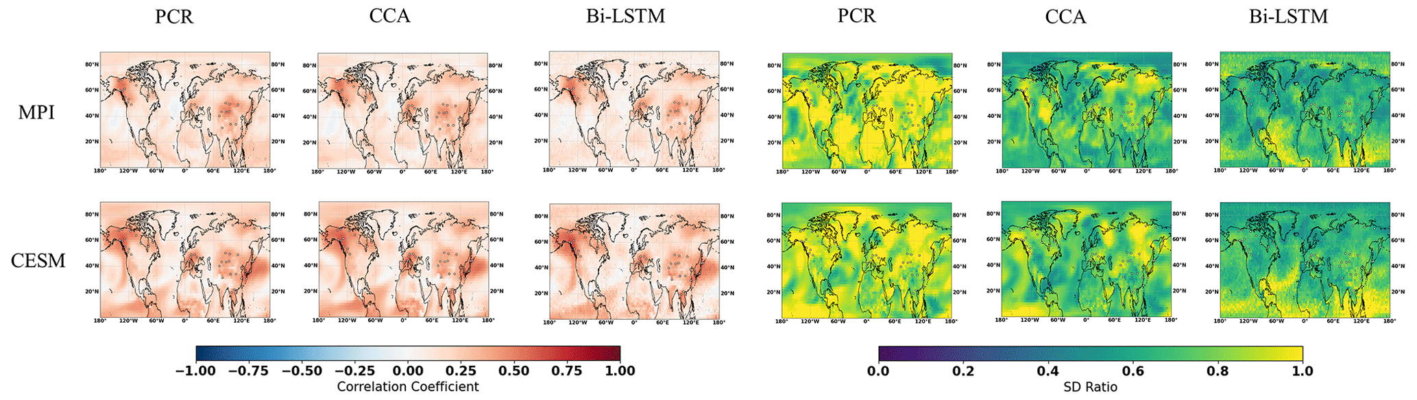
Figure 6The same as Fig. 5 but for employing the full 48-pseudoproxy network with white noise contamination.
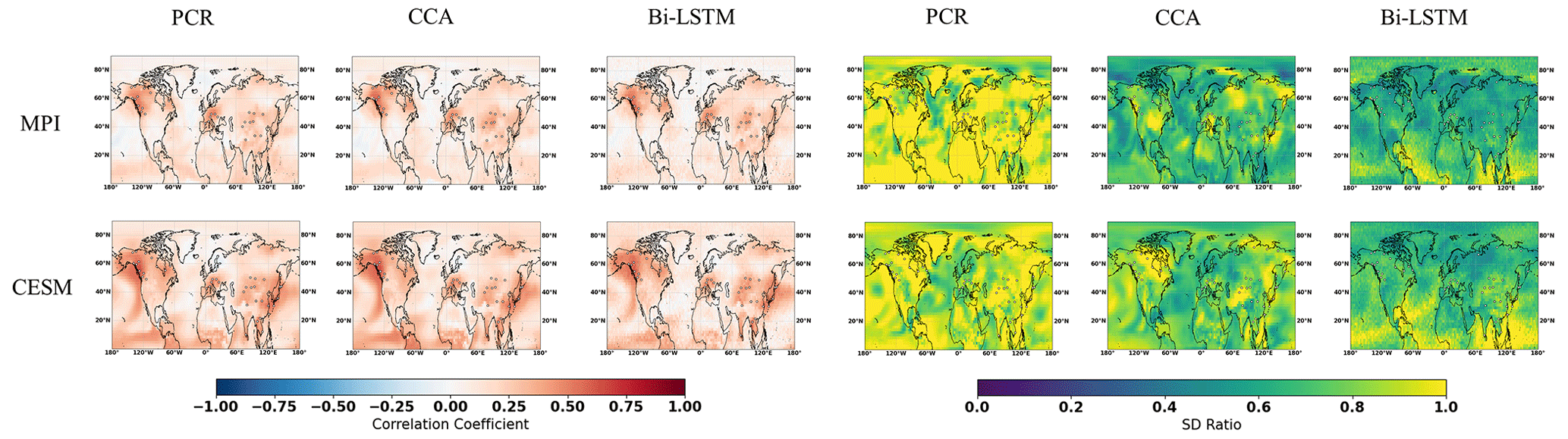
Figure 7The same as Fig. 5 but for employing the full 48-pseudoproxy network with red noise contamination.
The spatial cc maps for the ideal PPEs in NH are shown in Fig. 5. Again, all three CFR methodologies yield relatively similar spatial cc patterns of skill for each of the climate models employed here. Skillful reconstructions are again achieved over regions with a denser pseudoproxy network (over the North American and Eurasian regions). In addition, relatively high cc values also occur in tropical regions. A relatively high reconstructed skill is achieved over regions with fewer (or without) pseudoproxies, indicating that climate teleconnections between tropics and mid-latitude regions could be responsible for the reconstruction skill in tropical regions.
All derived CFRs suffer from underestimation of interannual variance, as shown in Fig. 5 and in Table 1, except that the PCR method presents a clearly interannual variance overestimation referring to the specific spatial SD ratio map in Fig. 5. This overestimation may be impacted by overfitting, since the number of predictors is 47 pseudoproxies and the calibration period spans 100 time steps. The spatial distributions of the SD ratio also vary between climate models and CFR methodologies. They are also spatially heterogeneous. The CCA method and Bi-LSTM generally preserve more variance over regions with denser pseudoproxies in both CESM and MPI model, and a relatively higher SD ratio appeared in tropical regions within Bi-LSTM-based PPEs shown in Fig. 5.
Table 1Skill reconstruction statistics for the Northern Hemisphere mean temperature in the verification period for ideal PPEs. The table shows the result for three CFR methods (PCR, CCA, and Bi-LSTM) and two climate models (MPI and CESM). The numbers in parentheses indicate the skill statistics of white-noise-contaminated and red-noise-contaminated (italics) PPEs.
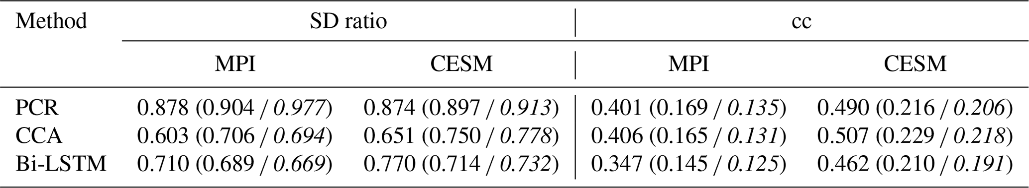
The CCA methodology seems to suffer more strongly from variance losses (see Table 1) over the entire NH compared to PCR and Bi-LSTM.
Considering the general methodological skill, as indicated by the derived spatial mean cc and SD ratio values in Table 1, the Bi-LSTM method presents relatively worse performance with lower mean cc. The methods PCR and Bi-LSTM generally outperform the CCA methodology, showing a higher mean SD ratio within ideal PPEs.
3.3 Spatially variability patterns of the reconstructed fields
In this section, we test the skill of the CFR in replicating the leading spatial patterns of variability, conducting an EOF analysis of the reconstructed temperature fields and compare them with the patterns derived from the target climate simulations. In our PPEs, the dominant patterns of temperature variability are assumed to be stationary. This assumption is also required in real climate reconstructions. Any non-stationarity would be reflected in a loss of reconstruction skill. This type of comparison is related to the tests performed by Yun et al. (2021). In this comparison, the PCA and CCA methods have a clear built-in advantage relative to the Bi-LSTM network, since these two methods operate by design in the space spanned by the leading EOFs of the temperature field. In the case of PCR, these reconstructed fields are a linear combination of the EOF patterns themselves. Therefore, so long as the reconstructed PC series remain uncorrelated, the EOFs of the reconstructed field will be exactly equal to the EOFs of the target climate simulations. Deviations from this behavior may be caused by the lack of strict orthogonality between the reconstructed PC series caused by the relationship between the proxies (predictors) and the PC series (predictands). However, it is reasonable to think that it would not be a priori surprising that the EOFs of the PCR-reconstructed fields would be similar to the original EOFs. The case for CCA is theoretically similar, but there are some potentially important points to bear in mind. The CCA patterns, which serve as a basis for the reconstructed field, are linear combinations of the original EOFs. These linear combinations may, for instance, not include the leading EOF of the original field, and thus the EOFs of the reconstructed field will not replicate the original leading EOF, even if the CCA series can be perfectly reconstructed by the proxy series. The third method (Bi-LSTM) is in this sense at a disadvantage relative to PCR and CCA, since the spatial covariance of the original field is not technically incorporated in its machinery. If the EOF patterns of the reconstructed field resemble the original EOF patterns, this would be an indication that the method itself is able to capture the main covariance patterns of the original field.
In order to have a deeper insight into the reconstruction performance of the three CFR methods, we calculated the four leading EOF patterns based on the results from the reconstruction interval and their proportion of explained variance of the reconstructed field derived from the three reconstruction method using the CESM pseudoproxies. The EOF patterns represented in Fig. 8 confirm the suggestion that the temperature reconstructed by the PCR and CCA methods (two lower rows in Fig. 8) very closely replicates the three leading patterns. The fourth EOF pattern displays some divergences from the original fourth pattern, but as we will show later, the variance explained by this fourth EOF is already rather low, meaning that the spatial pattern may be subject to statistical noise. More importantly, the Bi-LSTM method (second row) does produce EOF patterns that closely resemble the ones derived from the original field. This supports the idea that the method is able to replicate the spatial cross-covariance of the temperature field.
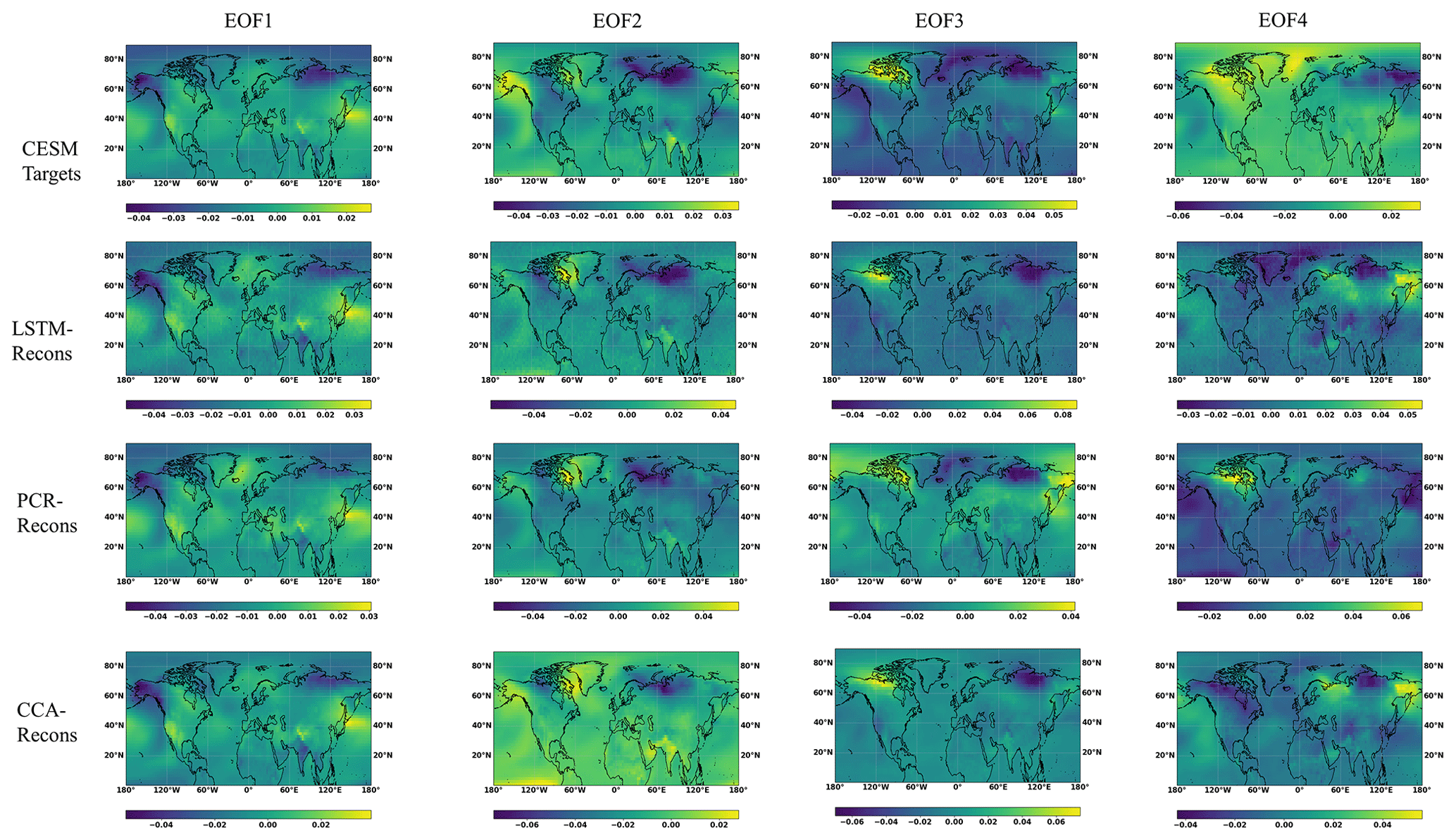
Figure 8The first four EOF patterns of the temperature field derived from CESM target, and from the temperature field reconstructed by the three methods-based ideal PPEs.
The corresponding spectrum of explained variance is displayed in Fig. 9. Here, the percentage of explained variance of each model is calculated as the ratio of the eigenvalue to the total variance of the original field. This is definition is in principle similar to the definition adopted by Yun et al. (2021), but there is one important difference. Yun et al. (2021), according to their methodological description, calculate the portion of explained variance of each mode as the ratio between the eigenvalue and the total variance of the respective field (either original or reconstructed). This choice could, however, cause a statistical artifact. For instance, when using the PCR regression method, we could choose to reconstruct only the leading EOF pattern. This pattern alone will explain 100 % of the reconstructed variance by definition, but this result would obviously be not informative. The choice of the total variance of the original field as reference thus leads to more informative results in general. The spectra for model simulation and three method-based ideal PPEs in this text are computed as the ratio between each of the first four reconstructed eigenvalues and the cumulative sum of all eigenvalues from the target variable.
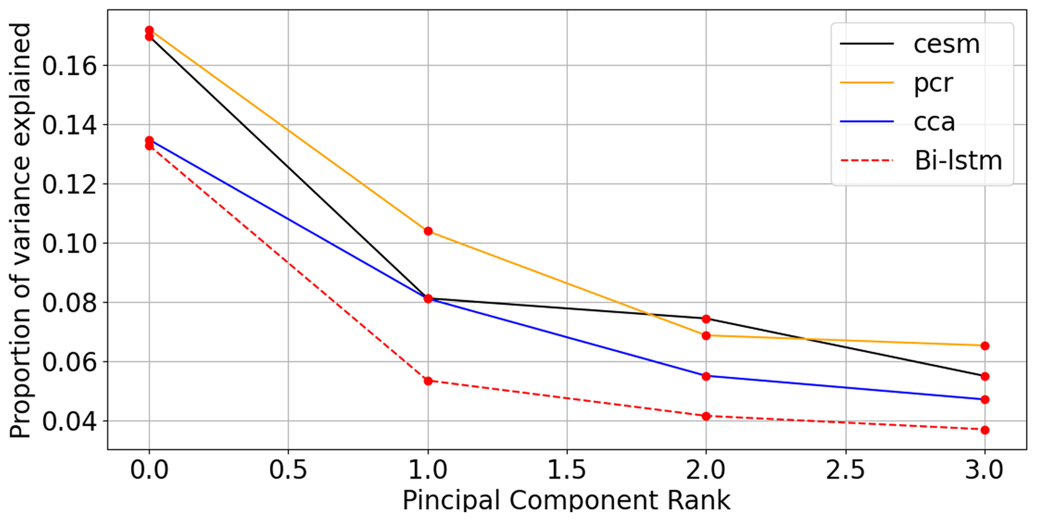
Figure 9Eigenvalue spectra for the CESM simulation and three method reconstructions: the spectra for the CESM simulation and three method-based ideal PPEs are computed as the ratio between each of the first four reconstructed eigenvalues and the cumulative sum of all eigenvalues from the target CESM model.
3.4 An alternative pseudoproxy network
In this section, we summarize a few additional experiments using the original locations of the PAGES network (Emile-Geay et al., 2017) instead of the filtered network used in previous experiments. In this section, we show only one model test bed for ideal, white noise, and red noise pseudoproxies. The results obtained with the MPI-ESM-M model are similar and are omitted here for the sake of brevity.
The reconstruction skill measured by cc and the SD ratio display similar spatial patterns to those obtained with network pre-selected according to the criteria of St. George (2014). As shown in Fig. 10, the derived correlations are generally higher over regions where denser pseudoproxy exists across both ideal and noisy PPEs, and weakly reconstructed correlations appeared over pseudoproxy-free regions. The PCR method presents a distinct interannual variance overestimation as shown in the specific spatial SD ratio map in Fig. 10 among ideal and noisy PPEs, while a clearly interannual variance overestimation also occurs in CCA-based CFRs in the noisy PPEs. A relatively reasonable SD ratio is revealed in tropical regions within Bi-LSTM-based PPEs shown in Fig. 10. In general, high reconstruction skills remain over regions where denser pseudoproxies exists based on this additional PAGES 2k pseudoproxy network.
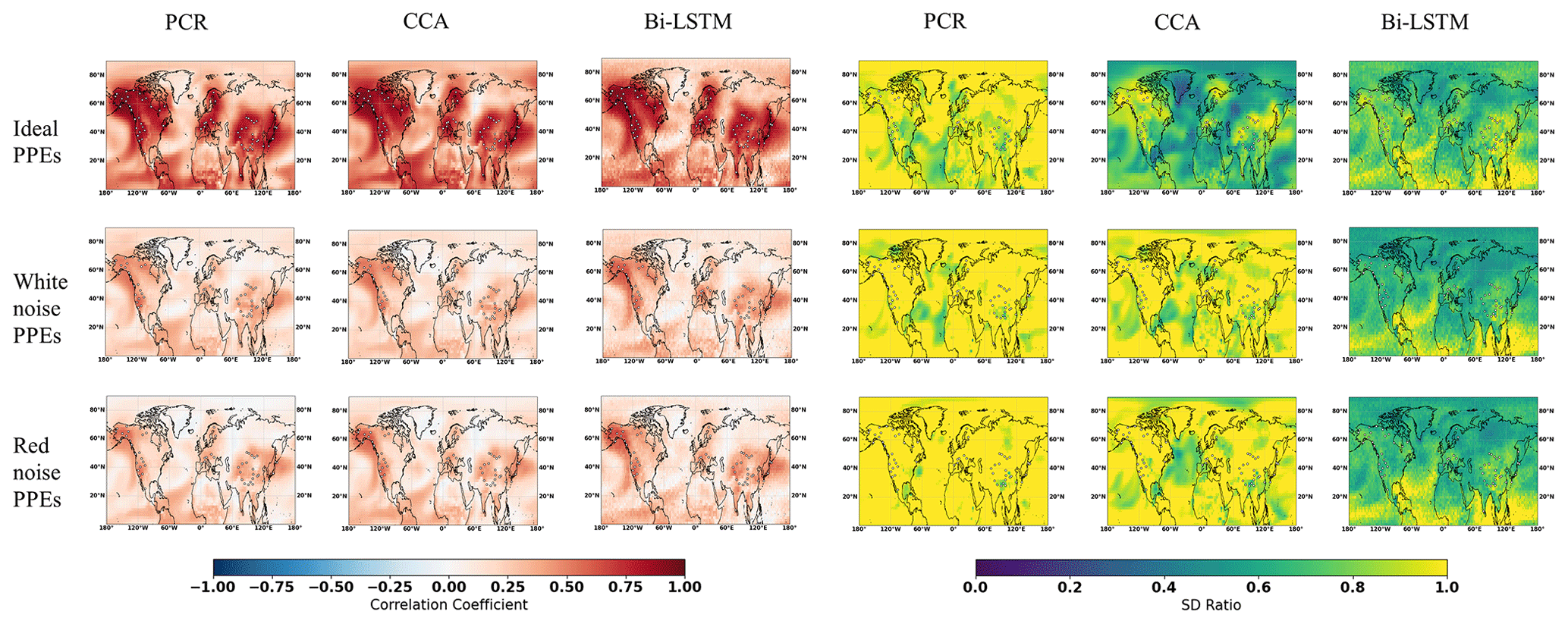
Figure 10Summary of the pseudo-reconstructions derived from the CESM model-based pseudoproxies using the original PAGES proxy network. The panels display the maps of the temporal correlation coefficients at the grid cell level (cc) and the ratio of standard deviations (SD ratio) between the reconstructed and target temperature fields.
3.5 Northern Hemisphere and AMV indices
The evolution of the decadal NH mean temperature anomalies reconstructed by the three CFR methodologies and using pseudoproxies from two models is illustrated in Fig. 11. All indices have been smoothed using a Butterworth low-pass filter to remove temporal fluctuations shorter than 10 years. The reconstruction performance varies among different the CFR methodologies. We will employ the correlation coefficient (cc), standard deviation (SD), and root-mean-square error (RMSE) as evaluation metrics for NH and AMV indices.
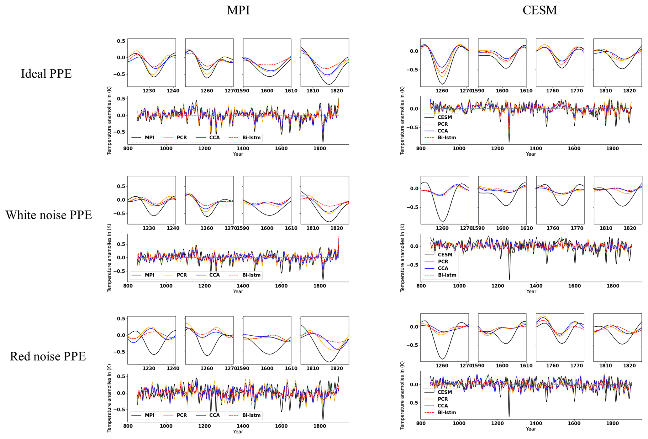
Figure 11Mean time series evolution of the validated reconstructions for the NH summer temperature anomaly using the full set of 48 pseudoproxies based on PCR, CCA, and Bi-LSTM CFR methods. All time series have been smoothed using a Butterworth low-pass filter to remove temporal fluctuations shorter than 10 years. MPI and CESM represent MPI/CESM model-simulated “true” climatology. We selected several reconstructed extreme cooling periods with a shorter interval (10-year periods are selected before and after the specific extreme cooling year) and plotted them above the indices subfigure of the entire reconstruction.
The temporal evolution of the original AMV indices (Fig. 12) differs among the simulations, reflecting the different forcings used in each simulation and the model-specific contribution of internal variability to the index variations (Wagner and Zorita, 2005; Schmidt et al., 2011). Considering the methodological performance, all three methods generally achieve good AMV index reconstructions when using perfect pseudoproxies, as shown in each panel of Fig. 12 and in Table 3.
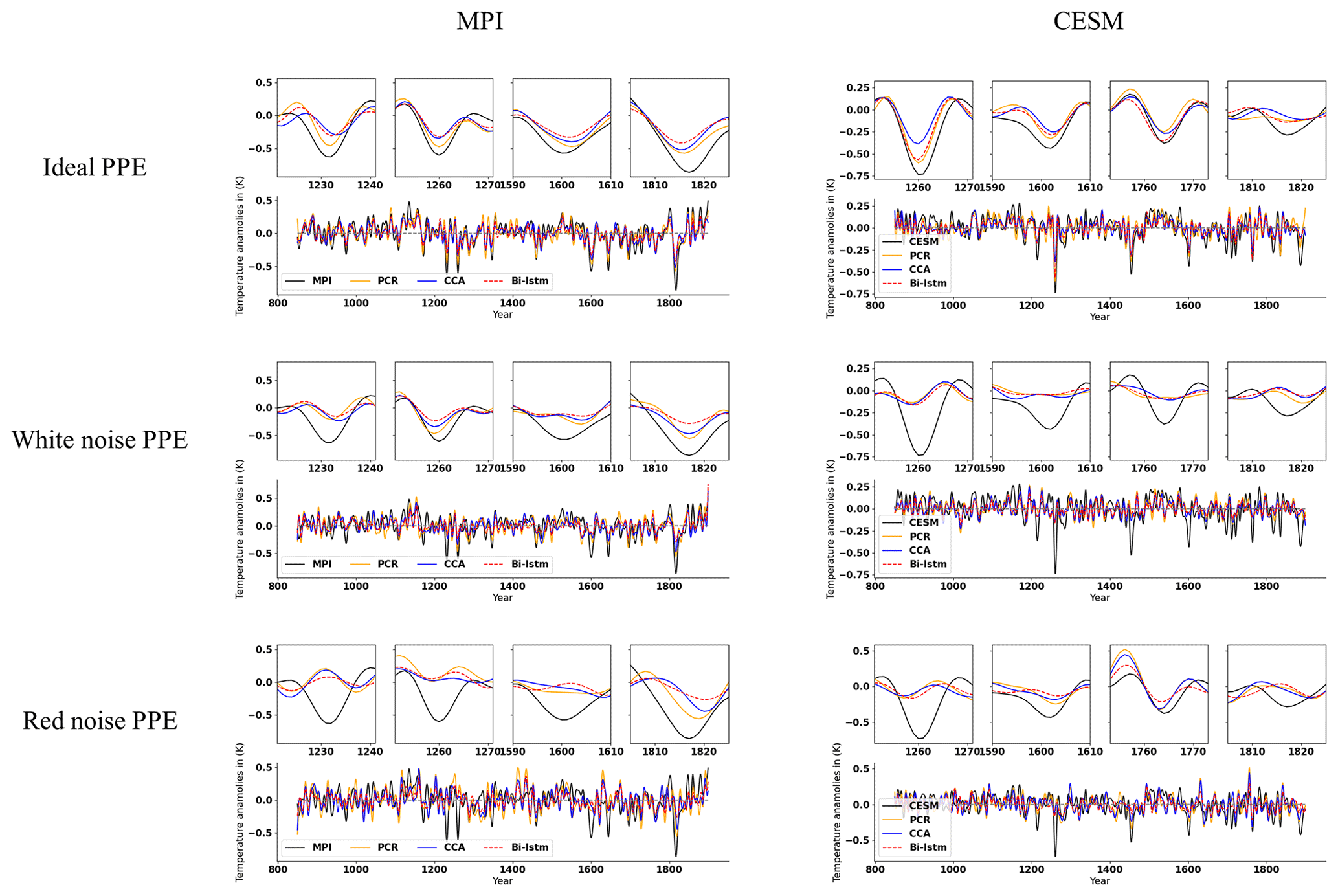
The NH and AMV indices derived from more realistic noise-contaminated CFRs are shown in Figs. 11 and 12, respectively. The larger noise contamination results in substantial skill deterioration (cc, SD, and RMSE displayed within brackets in Tables 2 and 3). All three methods generally fail to capture the complete variance of the target indices, and the magnitude of strong cooling phases is strongly underestimated.
Table 2The cc, SD, and RMSE (K) values during the verification interval for decadal NH mean temperature derived from ideal PPEs. The numbers in parentheses indicate skill statistics of white-noise-contaminated and red-noise-contaminated (italics) PPEs.
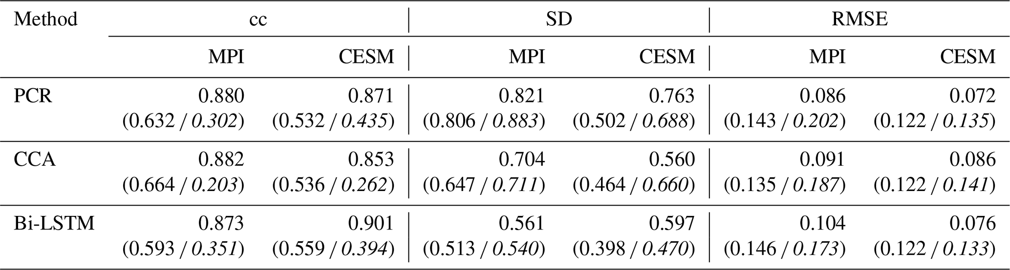
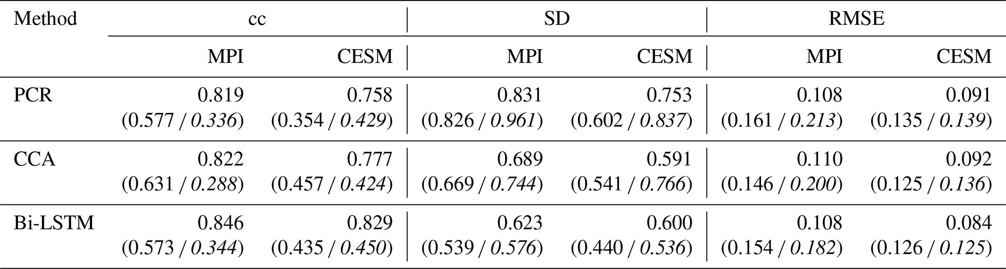
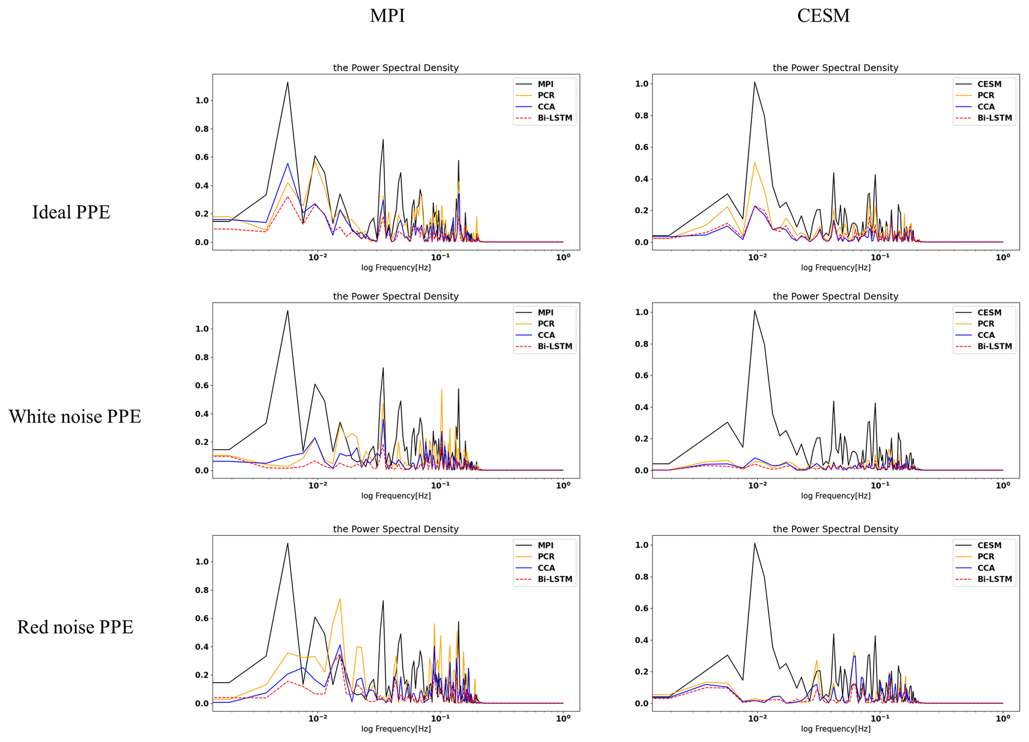
Figure 13 illustrates the comparison between reconstructions and target models of power spectral densities for Northern Hemisphere indices using both ideal and noise-contaminated PPEs. As indicated in Fig. 13, all three methods generally underestimate the power density, whereas this underestimation is more significant for the derived noise-contaminated PPE.
3.6 Probability distributions of reconstructed variables
Even though the three reconstruction methods tend to underestimate the overall variability when using noisy pseudoproxies, an interesting question is their skill when reproducing the probability distributions of the climate indices. A particularly relevant question is whether the methods are able to capture extreme phases of those indices.
Figures 14 and 15 display the histogram for the decadal NH mean and AMV indices, respectively. Each panel represents the histograms of reconstructed temperature indices across the three methods compared with the histograms of the target temperature index.
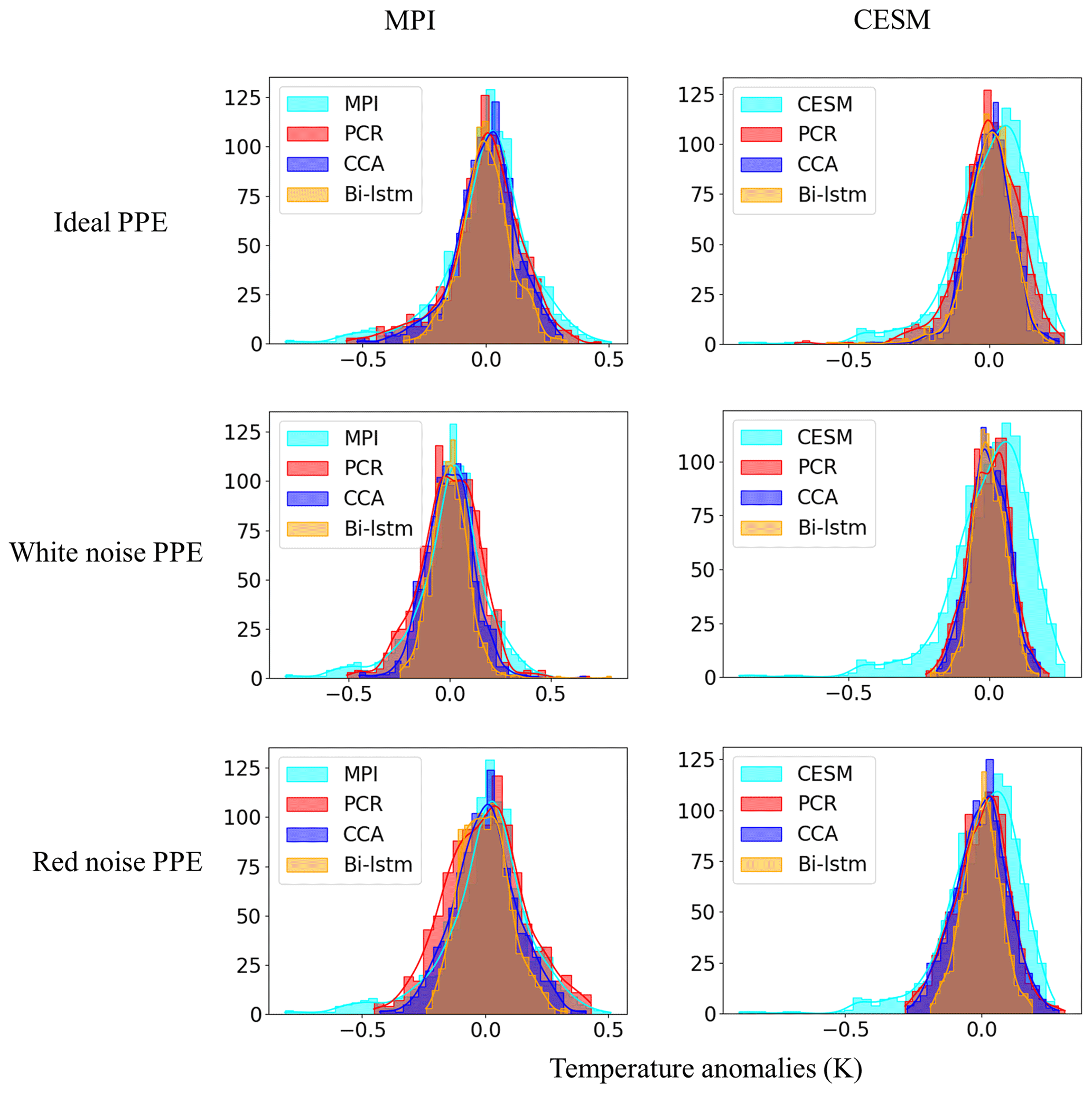
Figure 14Histogram for the decadal filtered NH mean index. The x axis denotes temperature anomaly values, and the y axis is the number of data points in each bin. A total of 30 bins are selected to plot each of the histograms.
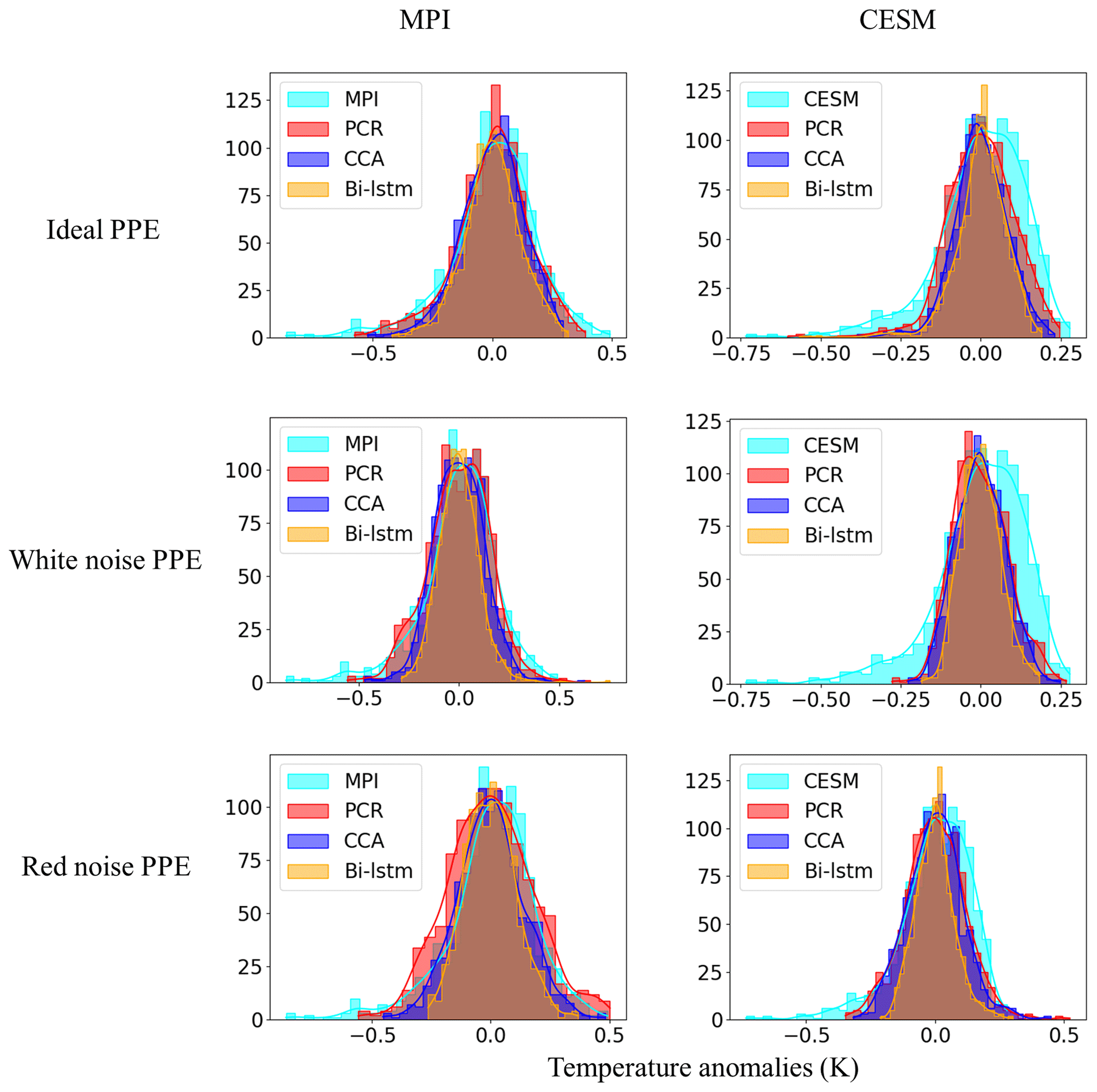
We quantify the distribution similarity between the reconstructed and target distributions for both NH and AMV indices using the two-sample Kolmogorov–Smirnov test as a metric (Hodges, 1958) (see Tables 4 and 5). A smaller value of the KS statistic indicates a stronger overall similarity between the two probability distributions. The smallest KS statistic is achieved by the PCR method (see Tables 4 and 5), confirming the impression that the PCR outperforms the other two methods for index reconstructions in both the ideal and noise-contaminated PPEs.
Table 4Kolmogorov–Smirnov test statistic and p value for quantifying the histogram distributions between model and reconstructed NH decadal means. Low values of the KS statistic indicate a larger similarity between the two distributions. The numbers in parentheses indicate the KS statistic and p value of white-noise-contaminated and red-noise-contaminated (italics) PPEs.
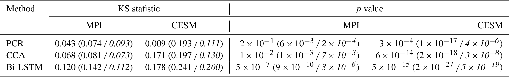
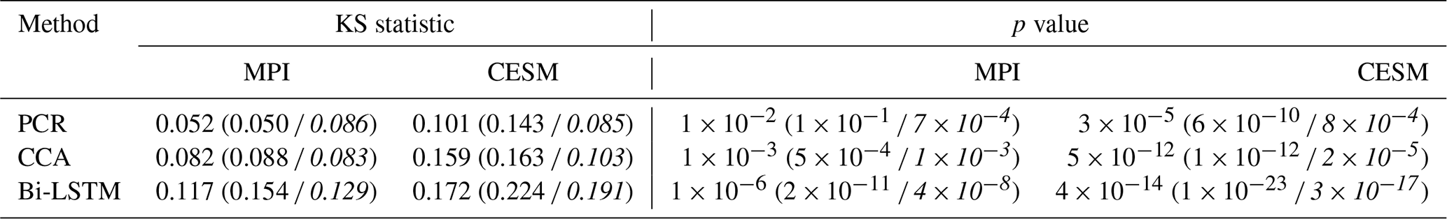
For perfect pseudoproxies, the PCR reconstruction seems to capture the overall target distribution best. It captures the lower tail better than CCA and the upper tail better than CCA and Bi-LSTM. The differences between the methods become smaller for the reconstructions with noisy pseudoproxies, with the PCR still being better than the other two methods (contaminated PPEs in Figs. 14 and 15). The Bi-LSTM performs worst for capturing the lower and upper tails of distribution among the three methods for both the NH mean and the AMV index.
3.7 Alternative architectures of the Bi-LSTM method
Although the design of machine-learning methods may be guided by physical considerations, machine-learning methods are still to a large extent a matter of trial and error. The complexity of the method hinders the disentangling of the causes as to why the methods behave in a certain way. Here, we explore the alternative architectures of the Bi-LSTM method to assess the resoluteness of the conclusions drawn from the basic design. We have explored varying network depths (number of layers), different learning rates, and different cost functions to optimize the network parameters, among other approaches. A summary of the results is included in Appendix B.
We could not recognize systematic effects in the skill in this set of different network designs. The skill varies rather randomly, and it is probable that the identification of optimal network architectures for this specific reconstruction question may not be something that can be extrapolated to other applications in paleoclimate. We settled for this application, on a heuristic basis, on an architecture with two hidden layers, 4000 hidden nodes, and a learning rate of 10−3, using the activation function Leaky ReLu, a batch size of 20, and the Huber loss function.
4.1 Nonlinear method performance
Our initial hypothesis was that a more sophisticated model might be able to better capture relationships that are more complex. For instance, a linear model cannot capture nonlinear links outside a narrow range of variations. An artificial neural network is a subset of a machine-learning method that can be understood as a universal approximator that can map and approximate any kind of function by selecting a suitable set of connecting weights and transfer functions (Hornik et al., 1989). Thus, it is reasonable to assume that a better representation of the links between proxy series and climate fields, and thus a better reconstruction performance, might be achieved.
The Bi-LSTM method is the most complex of the three tested in this study. Among these methods, it is also the only one that aims to capture serial dependencies. Our hypothesis was that better reconstruction skill could be achieved by the Bi-LSTM method. However, this is not the case in our pseudoproxy experiments. For the spatially resolved NAE fields, the nonlinear Bi-LSTM method achieves a similar skill to the linear PCR and CCA methods, both with ideal and noisy PPEs (see Figs. 2–4).
For the spatially resolved NH field, the PCR overestimates the variabilities both in ideal and noisy PPEs (see spatial SD ratio maps in Figs. 5–7 and mean statistics skills Table 1), and the CCA method shows relatively low overestimated variance in noisy PPEs, while Bi-LSTM presents relatively reasonable reconstructions without clear overestimation in both ideal and noisy PPEs (see Figs. 5–7 and Table 1). Among ideal PPEs across two models, the PCR is generally the best method among the three methods, and the nonlinear Bi-LSTM is second-best method, with a higher SD ratio and worse cc than the CCA method (see Figs. 5–7 and the mean skill statistics in Table 1). Both PCR and CCA exhibit overestimated reconstructions in the amplitude of climatic variability within noisy PPEs. Bi-LSTM presents relatively robust reconstructions (especially without variance overestimations) in noisy PPEs (see Figs. 5–7 and the mean skill statistics in Table 1), which may indicate that the LSTM method shows some degree of advantage when reproducing and keeping the general variance within noisy PPEs. The presence of larger noise amplitude causes a deterioration of the Bi-LSTM reconstructions. This may be due to the known sensitivity of this method to the presence of noise. In contrast, the PCR and CCA are less sensitive to the presence of unknowns and the skill may even improve in these settings. A possible reason is the aforementioned overfitting for these two linear methods. The presence of noise ameliorates the collinearity of the proxies given the limited sample size used for training.
For the area-mean indices, all three methods again exhibit generally similar skill. Nevertheless, the Bi-LSTM more strongly underestimates the amplitude of variabilities than PCR and CCA, especially over some extreme cooling phases. This underestimation is also generally model dependent (see the different reconstructed performances in Figs. 11 and 12). In general, the PCR methods achieved the best performance for both extreme cooling signal capture and indices reconstruction across the two models and among the three methods. The power spectral density plots in Fig. 13 provide a deep insight into these different reconstruction performances for NH temperature indices.
The general inability to capture the cooling extreme signals prior to the 20th century indicates that Bi-LSTM is not good at extrapolating to temperature ranges beyond the training set – a phenomenon that is intrinsic to most machine-learning-based methods.
Therefore, compared with the linear methods of PCR and CCA, the neural network model did not show clear advantages. The performance of Bi-LSTM might be further improved by optimizing the architecture and parameters of the network, including the type of objective function, type of neural activation function, network optimization function, number of hidden layers, and model learning rate. At this point, it would be quite natural to consider whether the selection or settings of these hyper-parameters in our study is optimal and to what extent the reconstruction skill is sensitive to changes in the hyper-parameters. Nadiga (2020) pointed out that the skill of some machine-learning methods is strongly dependent on these hyper-parameters. Machine-learning methods include an extensive range of complexity, and therefore it remains an open issue as to which machine-learning techniques are most suitable (or relatively suitable) for paleoclimate. It is not clear how the structure of the machine-learning methods can be systematically optimized. At the moment, there is still a considerable amount of “trial and error” in the design and connection of the neural layers. Here, we have tested the Bi-LSTM network with several different architecture settings, and we finally decided on a relatively optimal architecture with two separated hidden layers and evaluated its performance using CFR experiments, which could be seen as a preliminary trial. Our first implementation of the more complex Bi-LSTM method does not show superiority over CFRs, at least in our specific experiments, so we would like to draw an assumption that more complicated architecture might not be helpful for CFRs. In addition, a degradation of out-of-sample performance may well be expected when a limited dataset is used to train a neural network model (Najafabadi et al., 2015). Nevertheless, we would like to point out other methods, such as an Echo state network (ESN, Lukosevicius and Jaeger, 2009; Nadiga, 2020), for paleo-climate research. Both ESN and LSTM belong to the family of RNNs, but ESN is much simpler than LSTM (Lukosevicius and Jaeger, 2009) and has outperformed the RNN methods in other applications (Chattopadhyay et al., 2019; Nadiga, 2020). Preliminary pseudoproxy tests also indicate that this method may improve the deficiencies of the Bi-LSTM. It will be more thoroughly explored in a follow-up study.
Another reason to consider machine-learning methods is the nonlinearity of the link between proxies and climate fields. In this particular application with pseudoproxies, the implied link is probably close to linear. However, these can be different on other cases and might be the case for more complex problems (i.e., the reconstruction of proxy precipitation fields or other modes of natural variability such as the North Atlantic Oscillation or El Niño–Southern Oscillation). As such, machine-learning methods should not be excluded a priori from the portfolio of CFR methods because they can lead to more skillful reconstructions of climate.
4.2 Model and pseudoproxy network dependency
The evaluation of the reconstruction skill seems to depend as much on the reconstruction method as on the underlying climate model simulation from which the pseudoproxies were generated. The differences in skill for the same method with different climate model data is of the same order as the differences in skill for the different methods with the same climate model data. The performance of the method does not seem to depend on the domain of the reconstruction. The reconstructions generally behave similar for the NAE; nevertheless, they show some differences in the NH test cases, especially in the derived SD ratio patterns.
Considering the effects of noise contamination on the methodological performance, both the PCR and CCA methods exhibit overestimation in the amplitude of reconstructed variability (see the SD ratio patterns in Figs. 9 and 10 and the mean skills in Table 1). However, all methods suffer from lower correlation coefficients in the more realistic PPEs (white-noise-contaminated and red-noise-contaminated PPEs). The nonlinear Bi-LSTM method is more strongly impacted by noise contamination (Table 1).
We conclude that noise-contaminated datasets may cause obvious overestimations in the amplitude of reconstructed variability for the linear PCR and CCA methods. Some noise signals may deteriorate the reconstructions, but noise signals may also lead to good reconstructions. The performance of CFR reconstructions is affected by many factors, such as the proxy numbers and their spatial distributions, random noise signals introduced and added to certain important spatial proxy locations could have a significant effect on the overall spatial reconstruction. For the nonlinear machine-learning methods, most are very sensitive to external noise. Kalapanidas et al. (2003) and Atla et al. (2011) demonstrated that linear regression can achieve better results than nonlinear methods when considering noise sensitivity studies. Moreover, some studies indicated that external interference or noise could damage the ability of neural networks (Heaven, 2019), which may indicate that different or higher noise levels can lead to worse performance for the nonlinear machine-learning method LSTM.
From the perspective of the spatial coverage of the proxy network, the spatial cc and SD ratio patterns (except the PCR method) reveal the reconstruction skill over the entire NH region, although this skill is weaker in areas that are more poorly sampled by the pseudoproxy network (spatial cc patterns in Figs. 5–7). Interestingly, the tropical regions do show some reconstruction skill, especially in the derived reconstructions based on Bi-LSTM (spatial SD ratio patterns in Figs. 5–7) despite almost no pseudoproxies being located in the tropics. This result indicates the climate teleconnections between tropics and mid-latitude regions could lead to some indirect skill. However, the proxy networks and noise scenarios constructed in this context are certainly not able to completely mimic or simulate the full range of characteristics for climatic proxies in the real world.
A nonlinear Bi-LSTM neural network method to reconstruct North Atlantic—European and Northern Hemisphere temperature fields was tested with climate surrogate data generated by simulations with two different climate models. Compared to the more classical methods of linear principal component regression and canonical correlation analysis, the NAE and NH summer temperature field could be reasonably reconstructed using both linear and nonlinear methodologies referring to the spatial cc metric. In the relatively large spatial region of the NH temperature field, more discrepancies appeared in the reconstructions among different climate models and methods based on the derived spatial SD ratio metric. The conclusions drawn from this study can be summarized as follows.
-
In general, all three methods display similar skills when using ideal (noise-free) pseudoproxies, while in the more realistic PPEs (noise-contaminated PPEs) both the PCR and CCA method exhibit an overestimation of temperature variance preservation in contrast to the nonlinear Bi-LSTM method.
-
The pseudoproxy networks used in this study were mostly located in the extratropical regions, with only three proxies being located in the tropical area. All CFR methodologies produce generally good reconstructions in regions where dense pseudoproxy networks are available. Moreover, teleconnections are explored by these CFR methodologies, leading to some weak spatial reconstruction skills outside of the proxy-sampled regions (e.g., in the tropical region).
The classical linear-based PCR method generally outperforms the Bi-LSTM and CCA methods in both spatial and index reconstructions.
-
Here, we could draw a general conclusion that the nonlinear artificial neural network method (Bi-LSTM) employed herein is not superior for CFR reconstructions (at least in our PPEs). In general, Bi-LSTM shows worse skill in spatial and temporal CFRs than PCR and CCA and in capturing extremes. However, it is advisable to employ a larger set of nonlinear CFR methods to evaluate different model structures and to further test their performance on CFRs.
The simulation with the model MPI-ESM-P is not part of the standard CMIP5 simulation suite. In the following, we include additional technical details on this simulation. The MPI simulation was started from the year 100 BCE with restart files from 500-year spin-down simulation experiments forced with constant external conditions representing the year 100 BCE. After 100 BCE, variation in volcanic, solar, orbital, and greenhouse gas concentrations are implemented. Land usage was held constant until 850 CE, with conditions representing those for the year 850 CE. The variation in orbital parameters is calculated after the PMIP3 protocol (Schmidt et al., 2011). The solar activity has been rebuilt on the basis of the reconstruction of Vieira et al. (2011), employing the algorithm and scaling outlined in Schmidt et al. (2011), which corresponds to a difference in shortwave top-of-the-atmosphere insolation of 1.25 W m−2 (∼0.1 %) between the second half of the 20th century (1950–2000) and the Maunder Minimum (1645–1715 CE). Variations in greenhouse gas concentrations related to CO2, N2O, and CH4 follow the reconstruction of the PMIP3 protocol. The concentrations were held constant to the values of 1 CE between 100 BCE and 1 CE because the Law Dome records do not extend beyond the year 1 CE. After 1850 CE, a reconstructed aerosol loading following Eriksen Hammer et al. (2018) was also employed to account for transient anthropogenic aerosol emissions. The extension and reconstruction of the volcanic forcing is related to a rescaling of the newly available Sigl et al. (2015) dataset to match the reconstruction of Crowley and Unterman (2013). The large volcanoes at different latitudinal bands are rescaled according to sulfate concentrations, and the Crowley algorithm was also eventually applied to yield aerosol optical depths and effective radii for four latitudinal bands separated by 30∘.
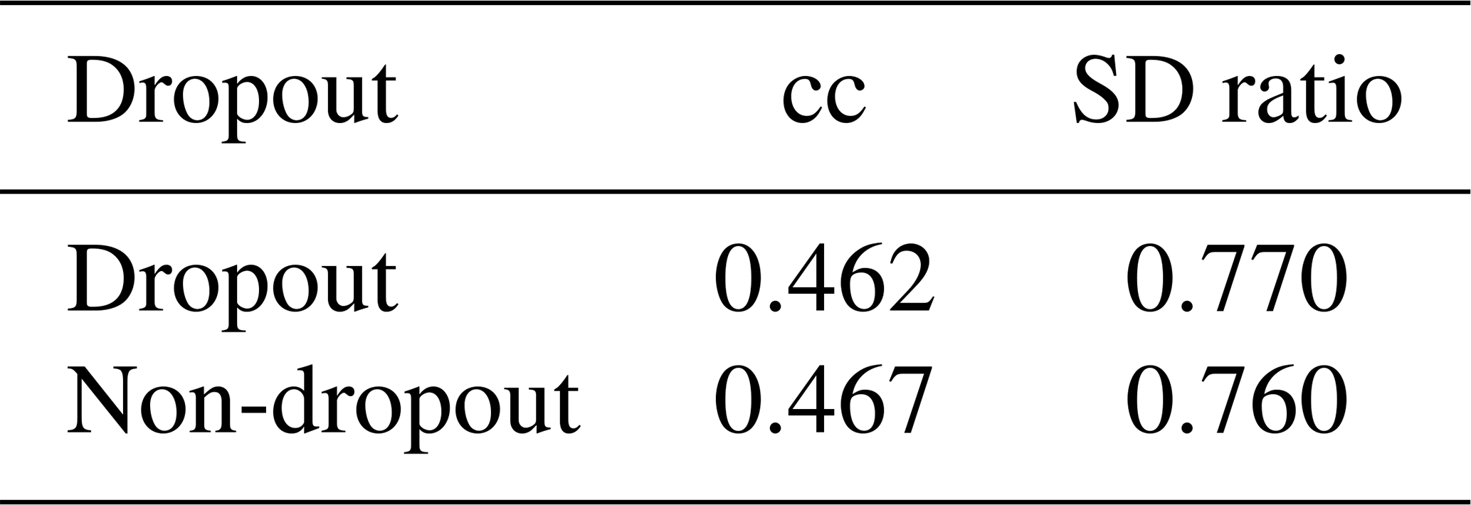
We have explored a range of Bi-LSTM architectures, including employing different network depths, introducing dropout layers, using different learning rates, and employing different loss functions to provide a more comprehensive evaluation of the Bi-LSTM method's performance and effectiveness. Tables B1–B6 present the reconstruction statistic skills for the spatial North Hemisphere mean temperature in the verification period for ideal PPEs based on CESM using different architecture settings of the Bi-LSTM method. In our PPE tests on paleo-CFRs, it seems that in this case we could not unequivocally identify optimal neural network structure that could universally outperform all others. The final Bi-LSTM architecture employed in our CFR experiments was finally determined and uses two hidden layers, 4000 hidden nodes, and a learning rate of 10−3, using the Leaky ReLu activation function, a batch size of 20, and the Huber loss function.
Table B1Different loss functions conditioned using other fixed parameters (two hidden layers, 4000 hidden nodes, and learning rate of 10−3, using the Leaky ReLu activation function and a batch size of 20).

MAE is the mean absolute error, MAPE is the mean absolute percentage error, MSE is the mean square error, and Huber is the Huber loss.
Table B2Different learning rates using Huber loss, with the rest of the parameters fixed as in Table B1.
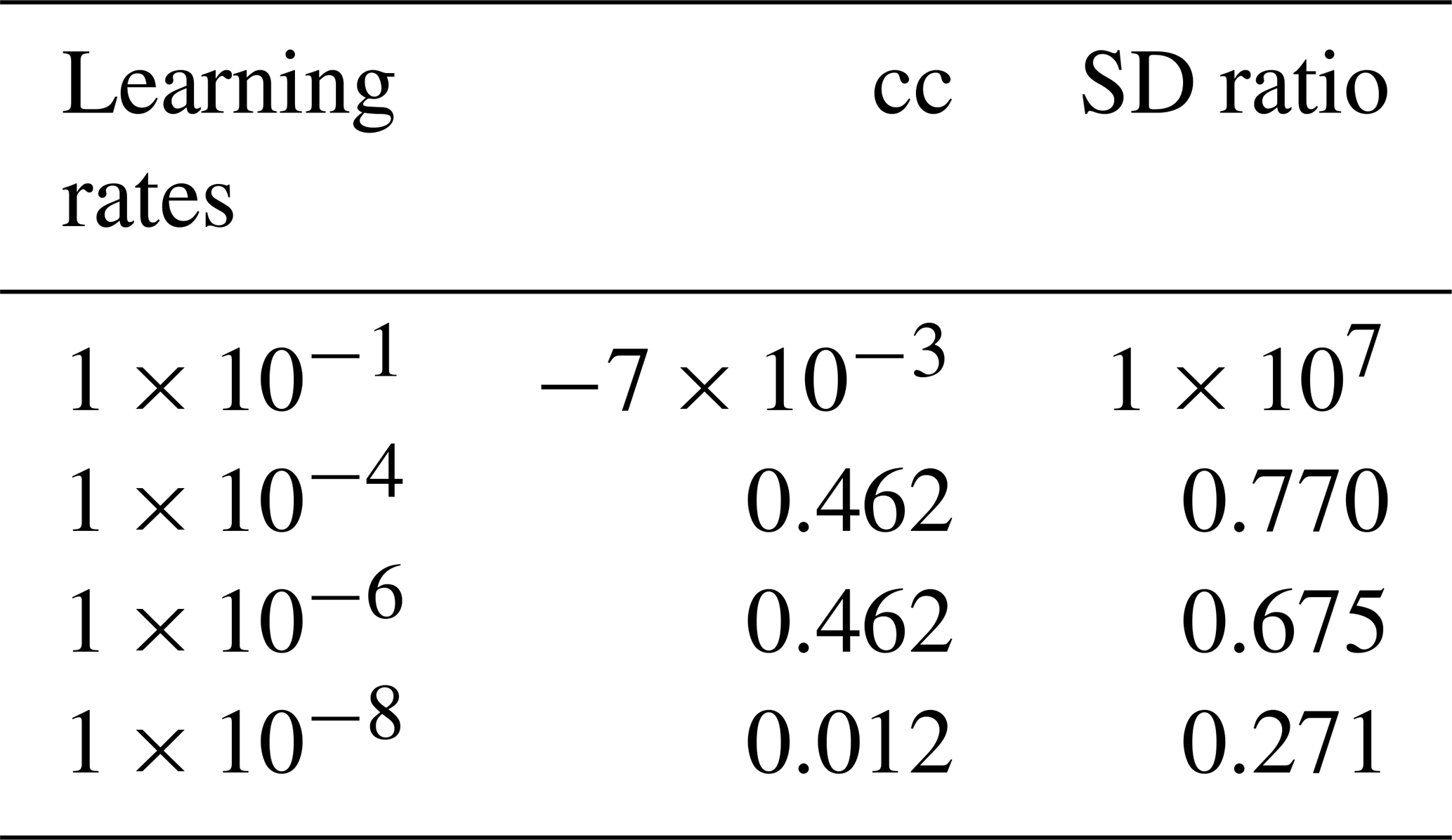
Table B3Different activation functions, with the rest of the parameters fixed as in Table B1.

Table B4Different hidden-layer amounts, with the rest of the parameters fixed as in Table B1.
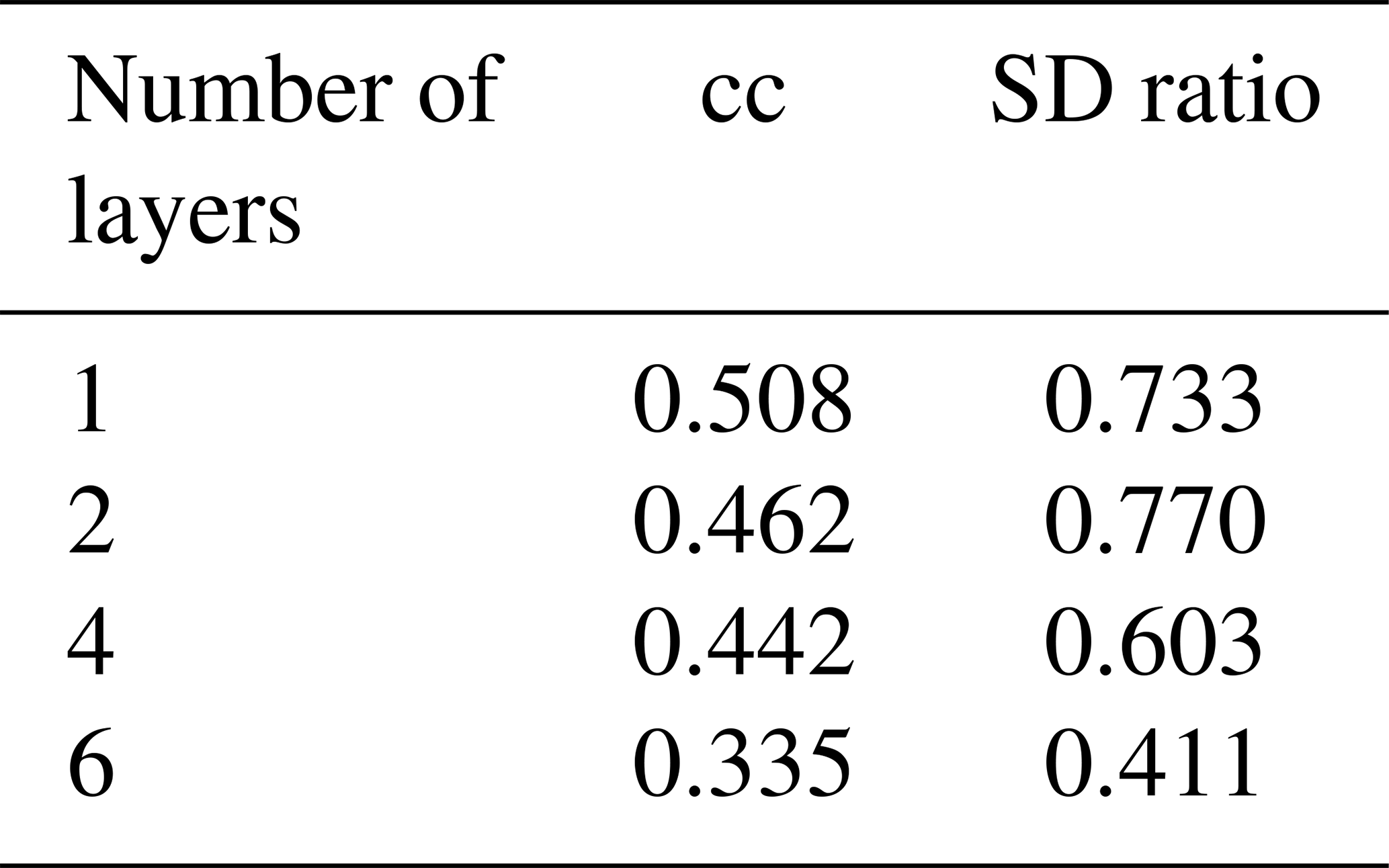
Table B5Different hidden-node amounts in each layer, with the rest of the parameters fixed as in Table B1.
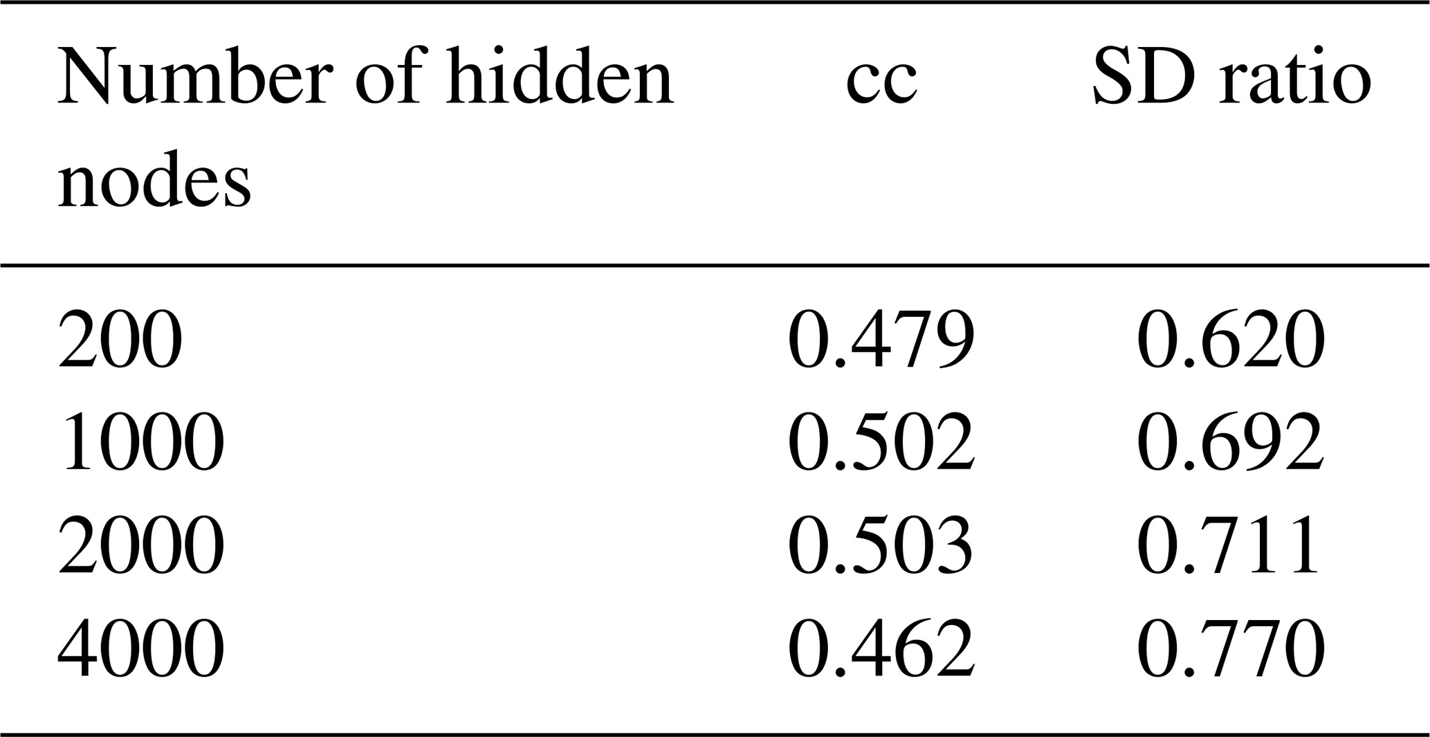
Table B6Example values with and without dropout layers having been conditioned, with the rest of the parameters fixed as in Table B1.
Appendix C displays the SD ratios for ideal pseudoproxies after filtering the reconstructed and target fields with a 30-year low-pass filter. At this timescales, the SD ratio is again lower than for the interannual variance.
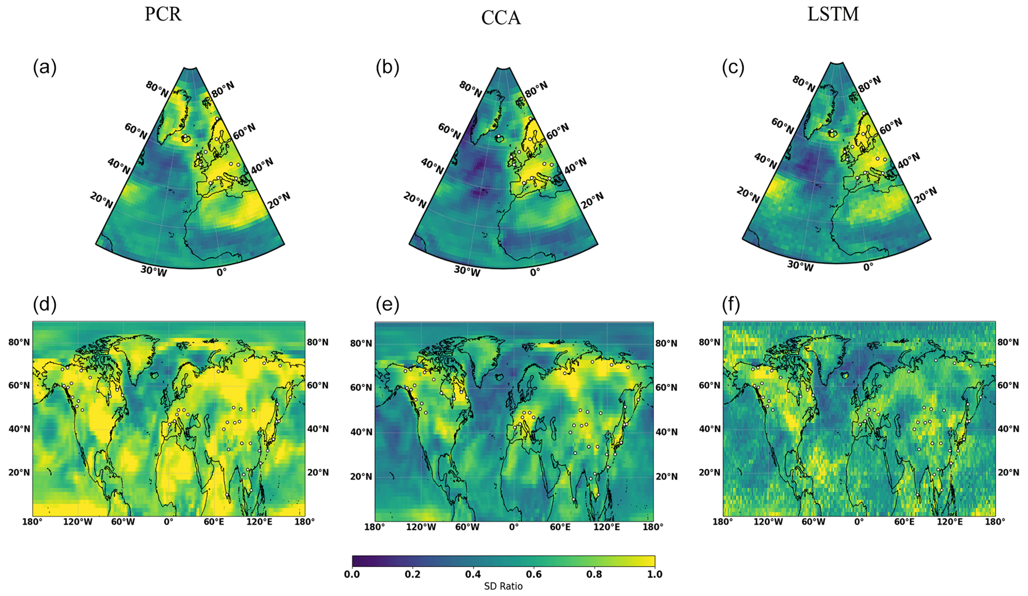
Figure C1The 30-year filtered SD ratio pattern using ideal PPEs based on the MPI model over the validation period (850–1899 CE) for the NAE (a–c) and NH (d–f) regions.
The MPI-ESM-P model output that was employed for this study is available upon request from the authors Sebastian Wagner or Eduardo Zorita and from the paleoclimatology data repository of the US National and Oceanic and Atmospheric Administration (https://www.ncei.noaa.gov/products/paleoclimatology; NCEI, 2022; Jungclaus et al., 2010). The CESM model data can be downloaded from https://www.cesm.ucar.edu/projects/community-projects/LME/ (NCAR, 2022; Otto-Bliesner et al., 2016).
The analysis was performed by ZZ with the consultation of SW, MK, and EZ. ZZ prepared the paper with contributions from all co-authors.
The contact author has declared that none of the authors has any competing interests.
Publisher's note: Copernicus Publications remains neutral with regard to jurisdictional claims in published maps and institutional affiliations.
The authors thank the MPI-ESM modeling groups participating in the CMIP5 initiative for providing their data and the CESM modeling group for making their data available. The authors thank the editor and the referees for constructive suggestions that have improved the content and presentation of this article.
This research has been supported by the China Scholarship Council (grant no. 201806570017).
The article processing charges for this open-access publication were covered by the Helmholtz-Zentrum Hereon.
This paper was edited by Steven Phipps and reviewed by two anonymous referees.
Amrhein, D. E., Hakim, G. J., and Parsons, L. A.: Quantifying structural uncertainty in paleoclimate data assimilation with an application to the Last Millennium, Geophys. Res. Lett., 47, e2020GL090485, https://doi.org/10.1029/2020GL090485, 2020.
Anchukaitis, K., Breitenmoser, P., Briffa, K., Buchwal, A., Büntgen, U., Cook, E., D'Arrigo, R., Esper, J., Evans, M., Frank, D., Grudd, H., Gunnarson, B., Hughes, M., Kirdyanov, A., Körner, C., Krusic, P., Luckman, B., Melvin, T., Salzer, M., Shashkin, A., Timmreck, C., Vaganov, E., and Wilson, R.: Tree-rings and volcanic cooling, Nat. Geosci., 5, 836–837, https://doi.org/10.1038/ngeo1645, 2012.
Anchukaitis, K. J., Wilson, R., Briffa, K. R., Büntgen, U., Cook, E. R., D'Arrigo, R., Davi, N., Esper, J., Frank, D., Gunnarson, B. E., Hegerl, G., Helama, S., Klesse, S., Krusic, P. J., Linderholm, H. W., Myglan, V., Osborn, T. J., Zhang, P., Rydval, M., Schneider, L., Schurer, A., Wiles, G., and Zorita, E.: Last millennium Northern Hemisphere summer temperatures from tree rings: Part II, spatially resolved reconstructions, Quaternary Sci. Rev., 163, 1–22, https://doi.org/10.1016/j.quascirev.2017.02.020, 2017.
Atla, A., Tada, R., Sheng, V., and Singireddy, N.: Sensitivity of different machine learning algorithms to noise, J. Comput. Sci. Coll., 26, 96–103, 2011.
Bengio, Y., Simard, P., and Frasconi, P.: Learning long-term dependencies with gradient descent is difficult, IEEE T. Neural Networ., 5, 157–166, 1994.
Biswas, K., Kumar, S., and Pandey, A. K.: Intensity Prediction of Tropical Cyclones using Long Short-Term Memory Network, arXiv [preprint], https://doi.org/10.48550/arXiv.2107.03187, 2021.
Biswas, S. and Sinha, M.: Performances of deep learning models for Indian Ocean wind speed prediction, Model. Earth Syst. Environ., 7, 809–831, https://doi.org/10.1007/s40808-020-00974-9, 2021.
Büntgen, U., Frank, D., Trouet, V., and Esper, J.: Diverse climate sensitivity of Mediterranean tree-ring width and density, Trees Struct. Funct., 24, 261–273, 2010.
Carrassi, A., Bocquet, M., Bertino, L., and Evensen, G.: Data Assimilation in the Geosciences: An overview on methods, issues, and perspectives, WIRes Clim. Change, 9, e535, https://doi.org/10.1002/wcc.535, 2018.
Chattopadhyay, A., Hassanzadeh, P., and Subramanian, D.: Data-driven predictions of a multiscale Lorenz 96 chaotic system using machine-learning methods: reservoir computing, artificial neural network, and long short-term memory network, Nonlin. Processes Geophys., 27, 373–389, https://doi.org/10.5194/npg-27-373-2020, 2020.
Christiansen, B.: Reconstructing the NH mean temperature: can underestimation of trends and variability be avoided?, J. Climate, 24, 674–692, 2011.
Christiansen, B. and Ljungqvist, F. C.: The extra-tropical Northern Hemisphere temperature in the last two millennia: reconstructions of low-frequency variability, Clim. Past, 8, 765–786, https://doi.org/10.5194/cp-8-765-2012, 2012.
Christiansen, B. and Ljungqvist, F. C.: Challenges and perspectives for large-scale temperature reconstructions of the past two millennia, Rev. Geophys., 55, 40–96, https://doi.org/10.1002/2016RG000521, 2017.
Coats, S., Smerdon, J. E., Cook, B. I., and Seager, R.: Stationarity of the tropical pacific teleconnection to North America in CMIP5/PMIP3 model simulations, Geophys. Res. Lett., 40, 4927–4932, https://doi.org/10.1002/grl.50938, 2013.
Crowley, T. J. and Unterman, M. B.: Technical details concerning development of a 1200 yr proxy index for global volcanism, Earth Syst. Sci. Data, 5, 187–197, https://doi.org/10.5194/essd-5-187-2013, 2013.
Cui, Z., Ke, R., Pu, Z., and Wang, Y.: Deep bidirectional and unidirectional LSTM recurrent neural network for network-wide traffic speed prediction, arXiv [preprint], https://doi.org/10.48550/arXiv.1801.02143, 2018.
Dueben, P. D. and Bauer, P.: Challenges and design choices for global weather and climate models based on machine learning, Geosci. Model Dev., 11, 3999–4009, https://doi.org/10.5194/gmd-11-3999-2018, 2018.
Emile-Geay, J., McKay, N. P., Kaufman, D. S., Von Gunten, L., Wang, J., Anchukaitis, K. J., and Henley, B. J.: A global multiproxy database for temperature reconstructions of the Common Era, Sci. Data, 4, 170088, https://doi.org/10.1038/sdata.2017.88, 2017.
Eriksen Hammer, S., Mertes, S., Schneider, J., Ebert, M., Kandler, K., and Weinbruch, S.: Composition of ice particle residuals in mixed-phase clouds at Jungfraujoch (Switzerland): enrichment and depletion of particle groups relative to total aerosol, Atmos. Chem. Phys., 18, 13987–14003, https://doi.org/10.5194/acp-18-13987-2018, 2018.
Evans, M., Smerdon, J. E., Kaplan, A., Tolwinski-Ward, S., and González-Rouco, J. F.: Climate field reconstruction uncertainty arising from multivariate and nonlinear properties of predictors, Geophys. Res. Lett., 41, 9127–9134, https://doi.org/10.1002/2014gl062063, 2014.
Folland, C. K., Knight, J., Linderholm, H. W., Fereday, D., Ineson, S., and Hurrell, J. W.: The Summer North Atlantic Oscillation: Past, present, and future, J. Climate, 22, 1082–1103, https://doi.org/10.1175/2008JCLI2459.1, 2009.
Frank, D., Esper, J., Zorita, E., and Wilson, R.: A noodle, hockey stick, and spaghetti plate: a perspective on high-resolution paleoclimatology, WIRes Clim. Change, 1, 507–516, 2010.
Gómez-Navarro, J. J., Zorita, E., Raible, C. C., and Neukom, R.: Pseudo-proxy tests of the analogue method to reconstruct spatially resolved global temperature during the Common Era, Clim. Past, 13, 629–648, https://doi.org/10.5194/cp-13-629-2017, 2017.
Goodfellow, I., Bengio, Y., and Courville, A.: Deep learning, MIT Press, ISBN 0262337371, 9780262337373, 2016.
Graves, A. and Schmidhuber, J.: Framewise phoneme classification with bidirectional LSTM and other neural and other neural network architectures, Neural Networks, 18, 602–610, https://doi.org/10.1016/j.neunet.2005.06.042, 2005.
Harlim, J.: Model error in data assimilation, in: Nonlinear and stochastic climate dynamics, edited by: Franzke, C. L. E. and O'Kane, T. J., Cambridge University Press, 276–317, https://doi.org/10.1017/9781316339251.011, 2017.
Heaven, D.: Why deep-learning AIs are so easy to fool, Nature, 574, 163–166, 2019.
Hegerl, G., Crowley, T., Hyde, W. T., and Frame, D. J.: Uncertainty in climate-sensitivity estimates (Reply), Nature, 446, E2, https://doi.org/10.1038/nature05708, 2007.
Hegerl, G. C., Crowley, T. J., Hyde, W. T., and Frame, D. J.: Climate sensitivity constrained by temperature reconstructions over the past seven centuries, Nature, 440, 1029–1032, https://doi.org/10.1038/nature04679, 2006.
Hernández, A., Martin-Puertas, C., Moffa-Sánchez, P., Moreno-Chamarro, E., Ortega, P., Blockley, S., Cobb, K. M., Comas-Bru, L., Giralt, S., Goosse, H., Luterbacher, J., Martrat, B., Muscheler, R., Parnell, A., Pla-Rabes, S., Sjolte, J., Scaife, A. A., Swingedouw, D., Wise, E., and Xu, G.: Modes of climate variability: Synthesis and review of proxy-based reconstructions through the Holocene, Earth Sci. Rev., 271, 103286, https://doi.org/10.1016/j.earscirev.2020.103286, 2020.
Hochreiter, S. and Schmidhuber, J.: Long short-term memory, Neural Comput., 9, 1735–1780, https://doi.org/10.1162/neco.1997.9.8.1735, 1997.
Hodges, J. L.: The significance probability of the Smirnov two-sample test, Ark. Mat., 3, 469–486, 1958.
Hornik, K., Stinchcombe, M., and White, H.: Multilayer feedforward networks are universal approximators, Neural Networks, 2, 359–366, https://doi.org/10.1016/0893-6080(89)90020-8, 1989.
Hotelling, H.: The relations of the newer multivariate statistical methods to factor analysis, Brit. J. Statist. Psych., 10, 69–76, https://doi.org/10.1111/j.2044-8317.1957.tb00179.x, 1957.
Huang, Y., Yang, L., and Fu, Z.: Reconstructing coupled time series in climate systems using three kinds of machine-learning methods, Earth Syst. Dynam., 11, 835–853, https://doi.org/10.5194/esd-11-835-2020, 2020.
Huntingford, C., Jeffers, E. S., Bonsall, M. B., Christensen, H. M., Lees, T., and Yang, H.: Machine learning and artificial intelligence to aid climate change research and preparedness, Environ. Res. Lett., 14, 124007, https://doi.org/10.1088/1748-9326/ab4e55, 2019.
Hurrell, J. W., Holland, M. M., Gent, P. R., Ghan, S., Kay, J. E., Kushner, P. J., Lamarque, J. F., Large, W. G., Lawrence, D., Lindsay, K., Lipscomb, W. H., Long, M. C., Mahowald, N., Marsh, D. R., Neale, R. B., Rasch, P., Vavrus, S., Vertenstein, M., Bader, D., Collins, W. D., Hack, J. J., Kiehl, J., and Marshall, S.: The Community Earth System Model: A Framework for Collaborative Research, B. Am. Meteorol. Soc., 94, 1339–1360, https://doi.org/10.1175/bams-d-12-00121.1, 2013.
Ilyina, T., Six, K. D., Segschneider, J., Maier-Reimer, E., Li, H., and Núñez-Riboni, I.: Global ocean biogeochemistry model HAMOCC: Model architecture and performance as component of the MPI-Earth system model in different CMIP5 experimental realizations, J. Adv. Model. Earth Sy., 5, 287–315, 2013.
Jacobeit, J., Wanner, H., Luterbacher, J., Beck, C., Philipp, A., and Sturm, K.: Atmospheric circulation variability in the NorthAtlantic-European area since the mid-seventeenth century, Clim. Dynam., 20, 341–352, https://doi.org/10.1007/s00382-002-0278-0, 2003.
Jahangir, H., Tayarani, H., Gougheri, S. S., Golkar, M. A., Ahmadian, A., and Elkamel, A.: Deep Learning-based Forecasting Approach in Smart Grids with Micro-Clustering and Bi-directional LSTM Network, IEEE T. Ind. Electron., 68, 8298–8309, https://doi.org/10.1109/TIE.2020.3009604, 2020.
Janjić, T., Bormann, N., Bocquet, M., Carton, J. A., Cohn, S. E., Dance, S. L., Losa, S. N., Nichols, N. K., Potthast, R., Waller, J. A., and Weston, P.: On the representation error in data assimilation, Q. J. Roy. Meteor. Soc., 144, 1257–1278, https://doi.org/10.1002/qj.3130, 2018.
Jones, P. D. and Mann, M. E.: Climate over past millennia, Rev. Geophys., 42, RG2002, https://doi.org/10.1029/2003RG0001433, 2004.
Jones, P. D., Briffa, K. R., Osborn, T. J., Lough, J. M., van Ommen, T. D., Vinther, B. M., Luterbacher, J., Wahl, E. R., Zwiers, F. W., Mann, M. E., Schmidt, G. A., Ammann, C. M., Buckley, B. M., Cobb, K. M., Esper, J., Goosse, H., Graham, N., Jansen, E., Kiefer, T., Kull, C., Küttel, M., Mosley-Thompson, E., Overpeck, J. T., Riedwyl, N., Schulz, M., Tudhope, A. W., Villalba, R., Wanner, H., Wolff, E., and Xoplaki, E.: Highresolution palaeoclimatology of the last millennium: A review of current status and future prospects, Holocene, 19, 3–49, https://doi.org/10.1177/0959683608098952, 2009.
Jungclaus, J. H., Lorenz, S. J., Timmreck, C., Reick, C. H., Brovkin, V., Six, K., Segschneider, J., Giorgetta, M. A., Crowley, T. J., Pongratz, J., Krivova, N. A., Vieira, L. E., Solanki, S. K., Klocke, D., Botzet, M., Esch, M., Gayler, V., Haak, H., Raddatz, T. J., Roeckner, E., Schnur, R., Widmann, H., Claussen, M., Stevens, B., and Marotzke, J.: Climate and carbon-cycle variability over the last millennium, Clim. Past, 6, 723–737, https://doi.org/10.5194/cp-6-723-2010, 2010.
Jungclaus, J. H., Fischer, N., Haak, H., Lohmann, K., Marotzke, J., Matei, D., Mikolajewicz, U., Notz, D., and von Storch, J. S.: Characteristics of the ocean simulations in MPIOM, the ocean component of the MPI-Earth system model, J. Adv. Model. Earth Sy., 5, 422–446, https://doi.org/10.1002/jame.20023, 2013.
Kalapanidas, E., Avouris, N., Craciun, M., and Neagu, D.: Machine Learning Algorithms: A Study on Noise Sensitivity, in: Proceedings of the First Balkan Conference in Informatics, Thessaloniki, Greece, 21–23 November 2003, 356–365, ISBN 9789602870457, 9602870451, 2003.
Kingma, D. and Ba, J.: Adam: a method for stochastic optimization, arXiv [preprint], https://doi.org/10.48550/arXiv.1412.6980, 2014.
Knerr, S., Lé, P., and Dreyfus, G.: Single-layer learning revisited: a stepwise procedure for building and training a neural network, in: Neurocomputing, Springer, Berlin, Heidelberg, 41–50, https://doi.org/10.1007/978-3-642-76153-9_5, 1990.
Knight, J. R., Folland, C. K., and Scaife, A. A.: Climate impacts of the Atlantic Multidecadal Oscillation, Geophys. Res. Lett., 33, L17706, https://doi.org/10.1029/2006GL026242, 2006.
Larsen, C. and MacDonald, G.: Relations between tree-ring widths, climate, and annual area burned in the boreal forest of Alberta, Can. J. Forest Res., 25, 1746–1755, 1995.
Lindgren, A., Lu, Z., Zhang, Q., and Hugelius, G.: Reconstructing past global vegetation with random forest machine learning, sacrificing the dynamic response for robust results, J. Adv. Model. Earth Sy., 13, e2020MS002200, https://doi.org/10.1029/2020MS002200, 2021.
Lukoševičius, M. and Jaeger, H.: Reservoir computing approaches to recurrent neural network training, Comput. Sci. Rev., 3, 127–149, https://doi.org/10.1016/j.cosrev.2009.03.005, 2009.
Luterbacher, J., Dietrich, D., Xoplaki, E., Grosjean, M., and Wanner, H.: European seasonal and annual temperature variability, trends, and extremes since 1500, Science, 303, 1499–1503, https://doi.org/10.1126/science.1093877, 2004.
Luterbacher, J., Werner, J. P., Smerdon, J. E., Fernández-Donado, L., González-Rouco, F. J., Barriopedro, D., Ljungqvist, F. C., Büntgen, U., Zorita, E., Wagner, S., Esper, J., McCarroll, D., Toreti, A., Frank, D., Jungclaus, J. H., Barriendos, M., Bertolin, C., Bothe, O., Brázdil, R., Camuffo, D., Dobrovolný, P., Gagen, M., García-Bustamante, E., Ge, Q., Gómez-Navarro, J. J., Guiot, J., Hao, Z., Hegerl, G. C., Holmgren, K., Klimenko, V. V., Martín-Chivelet, J., Pfister, C., Roberts, N., Schindler, A., Schurer, A., Solomina, O., von Gunten, L., Wahl, E., Wanner, H., Wetter, O., Xoplaki, E., Yuan, N., Zanchettin, D., Zhang, H., and Zerefos, C.: European summer temperatures since Roman times, Environ. Res. Lett., 11, 024001, https://doi.org/10.1088/1748-9326/11/2/024001, 2016.
Mann, M. E. and Jones, P. D.: Global surface temperatures over the past two millennia, Geophys. Res. Lett., 30, 1820, https://doi.org/10.1029/2003GL017814, 2003.
Mann, M. E. and Rutherford, S.: Climate reconstruction using “Pseudoproxies”, Geophys. Res. Lett., 29, 1501, https://doi.org/10.1029/2001GL014554, 2002.
Mann, M. E., Bradley, R. S., and Hughes, M. K.: Global-scale temperature patterns and climate forcing over the past six centuries, Nature, 392, 779–787, https://doi.org/10.1038/33859, 1998.
Mann, M. E., Rutherford, S., Wahl, E., and Ammann, C.: Testing the fidelity of methods used in proxy-based reconstructions of past climate, J. Climate, 18, 4097–4107, https://doi.org/10.1175/JCLI3564.1, 2005.
Mann, M. E., Rutherford, S., Wahl, E., and Ammann, C.: Robustness of proxy-based climate field reconstruction methods, J. Geophys. Res.-Atmos., 112, D12109, https://doi.org/10.1029/2006JD008272, 2007.
Mann, M. E., Zhang, Z., Hughes, M. K., Bradley, R. S., Miller, S. K., Rutherford, S., and Ni, F.: Proxy-based reconstructions of hemispheric and global surface temperature variations over the past two millennia, P. Natl. Acad. Sci. USA, 105, 13252–13257, https://doi.org/10.1073/pnas.0805721105, 2008.
Mann, M. E., Woodruff, J. D., Donnelly, J. P., and Zhang, Z.: Atlantic hurricanes and climate over the past 1,500 yr, Nature, 460, 880–883, https://doi.org/10.1038/nature08219, 2009a.
Mann, M. E., Zhang, Z., Rutherford, S., Bradley, R. S., Hughes, M. K., Shindell, D., Ammann, C., Faluvegi, G., and Ni, F.: Global signatures and dynamical origins of the Little Ice Age and Medieval Climate Anomaly, Science, 326, 1256–1260, https://doi.org/10.1126/science.1177303, 2009b.
Meyer, G. P.: An Alternative Probabilistic Interpretation of the Huber Loss, arXiv [preprint], https://doi.org/10.48550/arXiv.1911.02088, 2020.
Michel, S., Swingedouw, D., Chavent, M., Ortega, P., Mignot, J., and Khodri, M.: Reconstructing climatic modes of variability from proxy records using ClimIndRec version 1.0, Geosci. Model Dev., 13, 841–858, https://doi.org/10.5194/gmd-13-841-2020, 2020.
Nadiga, B.: Reservoir Computing as a Tool for Climate Predictability Studies, J. Adv. Model. Earth Sy., 13, e2020MS002290, https://doi.org/10.1029/2020MS002290, 2020.
Najafabadi, M. M., Villanustre, F., Khoshgoftaar, T. M., Seliya, M., Wald, R., and Muharemagic, E.: Deep learning applications and challenges in big data analytics, J. Big Data, 2, 1, https://doi.org/10.1186/s40537-014-0007-7, 2015.
NCAR: Last Millennium Ensemble Project (LME), https://www.cesm.ucar.edu/projects/community-projects/LME/, last access: 15 January 2022.
NCEI: Paleoclimatology, https://www.ncei.noaa.gov/products/paleoclimatology, last access: 10 January 2022.
Neale, R. B., Richter, J., Park, S., Lauritzen, P. H., Vavrus, S. J., Rasch, P. J., and Zhang, M.: The mean climate of the Community Atmosphere Model (CAM4) in forced SST and fully coupled experiments, J. Climate, 26, 5150–5168, https://doi.org/10.1175/JCLI-D-12-00236.1, 2013.
Otto-Bliesner, B. L., Brady, E. C., Fasullo, J., Jahn, A., Landrum, L., Stevenson, S., Rosenbloom, N., Mai, A., and Strand, G.: Climate Variability and Change since 850 CE An Ensemble Approach with the Community Earth System Model, B. Am. Meteorol. Soc., 97, 735–754, https://doi.org/10.1175/bams-d-14-00233.1, 2016.
Parsons, L. A., Amrhein, D. E., Sanchez, S. C., Tardif, R., Brennan, M. K., and Hakim, G. J.: Do Multi-Model Ensembles Improve Reconstruction Skill in Paleoclimate Data Assimilation?, Earth Space Sci., 8, e2020EA001467, https://doi.org/10.1029/2020EA001467, 2021.
Po-Chedley, S., Santer, B. D., Fueglistaler, S., Zelinka, M., Cameron-Smith, P., Painter, J., and Fu, Q.: Natural variability contributes to model-satellite differences in tropical tropospheric warming, Proc. Natl. Acad. Sci. USA, 118, e2020962118, https://doi.org/10.1073/pnas.2020962118, 2020.
Pyrina, M., Wagner, S., and Zorita, E.: Pseudo-proxy evaluation of climate field reconstruction methods of North Atlantic climate based on an annually resolved marine proxy network, Clim. Past, 13, 1339–1354, https://doi.org/10.5194/cp-13-1339-2017, 2017.
Qasmi, S., Cassou, C., and Boé, J.: Teleconnection Between Atlantic Multidecadal Variability and European Temperature: Diversity and Evaluation of the Coupled Model Intercomparison Project Phase 5 Models, Geophys. Res. Lett., 44, 140–149, https://doi.org/10.1002/2017GL074886, 2017.
Ramachandran, P., Zoph, B., and Le, Q. V.: Searching for activation functions, arXiv [preprint], https://doi.org/10.48550/arXiv.1710.05941, 2017.
Rasp, S. and Lerch, S.: Neural Networks for Postprocessing Ensemble Weather Forecasts, Mon. Weather Rev., 146, 3885–3900, https://doi.org/10.1175/MWR-D-18-0187.1, 2018.
Reick, C. H., Raddatz, T., Brovkin, V., and Gayler, V.: Representation of natural and anthropogenic land cover change in MPIESM, J. Adv. Model. Earth Sy., 5, 459–482, https://doi.org/10.1002/jame.20022, 2013.
Rolnick, D., Donti, P. L., Kaack, L. H., Kochanski, K., Lacoste, A., Sankaran, K., Ross, A. S., Milojevic-Dupont, N., Jaques, N., Waldman-Brown, A., Luccioni, A., Maharaj, T., Sherwin, E. D., Mukkavilli, S. K., Kording, K. P., Gomes, C., Ng, A. Y., Hassabis, D., Platt, J. C., Creutzig, F., Chayes, J., and Bengio, Y.: Tackling climate change with machine learning, arXiv [preprint], https://doi.org/10.48550/arXiv.1906.05433, 2019.
Schmidt, G. A.: Enhancing the relevance of paleoclimatic model/data comparisons for assessments of future climate change, J. Quaternary Sci., 25, 79–87, https://doi.org/10.1002/jqs.1314, 2010.
Schmidt, G. A., Jungclaus, J. H., Ammann, C. M., Bard, E., Braconnot, P., Crowley, T. J., Delaygue, G., Joos, F., Krivova, N. A., Muscheler, R., Otto-Bliesner, B. L., Pongratz, J., Shindell, D. T., Solanki, S. K., Steinhilber, F., and Vieira, L. E. A.: Climate forcing reconstructions for use in PMIP simulations of the last millennium (v1.0), Geosci. Model Dev., 4, 33–45, https://doi.org/10.5194/gmd-4-33-2011, 2011.
Schneider, T., Lan, S., Stuart, A., and Teixeira, J.: Earth System Modeling 2.0: A Blueprint for Models That Learn From Observations and Targeted High-Resolution Simulations, Geophys. Res. Lett., 44, 12396–12417, https://doi.org/10.1002/2017GL076101, 2018.
Schurer, A. P., Hegerl, G. C., Mann, M. E., Tett, S. F. B., and Phipps, S. J.: Separating forced from chaotic climate variability over the past millennium, J. Climate, 26, 6954–6973, https://doi.org/10.1175/JCLI-D-12-00826.1, 2013.
Schurer, A. P., Tett, S. F. B., and Hegerl, G. C.: Small influence of solar variability on climate over the past millennium, Nat. Geosci., 7, 104–108, https://doi.org/10.1038/ngeo2040, 2014.
Sigl, M., Winstrup, M., McConnell, J. R., Welten, K. C., Plunkett, G., Ludlow, F., Büntgen, U., Caffee, M., Chellman, N., Dahl-Jensen, D., Fischer, H., Kipfstuhl, S., Kostick, C., Maselli, O. J., Mekhaldi, F., Mulvaney, R., Muscheler, R., Pasteris, D. R., Pilcher, J. R., Salzer, M., Schüpbach, S., Steffensen, J. P., Vinther, B. M., and Woodruff, T. E.: Timing and climate forcing of volcanic eruptions for the past 2,500 years, Nature, 523, 543–549, https://doi.org/10.1038/nature14565, 2015.
Smerdon, J. E.: Climate models as a test bed for climate reconstruction methods: pseudoproxy experiments, WIRes Clim. Change, 3, 63–77, https://doi.org/10.1002/wcc.149, 2012.
Smerdon, J. E. and Pollack, H. N.: Reconstructing Earth's surface temperature over the past 2000 years: the science behind the headlines, WIRes Clim. Change, 7, 746–771, https://doi.org/10.1002/wcc.418, 2016.
Smerdon, J. E., Kaplan, A., Chang, D., and Evans, M. N.: A pseudoproxy evaluation of the CCA and RegEM methods for reconstructing climate fields of the last millennium, J. Climate, 23, 4856–4880, https://doi.org/10.1175/2010JCLI3328.1, 2010.
Smerdon, J. E., Kaplan, A., Zorita, E., Gonzalez-Rouco, J. F., and Evans, M. N.: Spatial performance of four climate field reconstruction methods targeting the Common Era, Geophys. Res. Lett., 38, L11705, https://doi.org/10.1029/2011GL047372, 2011.
Smerdon, J. E., Cook, B. I., Cook, E. R., and Seager, R.: Bridging past and future climate across paleoclimatic reconstructions, observations, and models: a hydroclimate case study, J. Climate, 28, 3212–3231, https://doi.org/10.1175/jcli-d-14-00417.1, 2015.
Smerdon, J. E., Coats, S., and Ault, T. R.: Model-dependent spatial skill in pseudoproxy experiments testing climate field reconstruction methods for the Common Era, Clim. Dynam., 46, 1921–1942, https://doi.org/10.1007/s00382-015-2684-0, 2016.
Steiger, N. J., Hakim, G. J., Steig, E. J., Battisti, D. S., and Roe, G. H.: Assimilation of time-averaged pseudoproxies for climate reconstruction, J. Climate, 27, 426–441, https://doi.org/10.1175/JCLI-D-12-00693.1, 2014.
Stevens, B., Giorgetta, M., Esch, M., Mauritsen, T., Crueger, T., Rast, S., Salzmann, M., Schmidt, H., Bader, J., Block, K., Brokopf, R., Fast, I., Kinne, S., Kornblueh, L., Lohmann, U., Pincus, R., Reichler, T., and Roeckner, E.: Atmospheric component of the MPI-M Earth System Model: ECHAM6-HAM2, J. Adv. Model. Earth Sy., 5, 146–172, https://doi.org/10.1002/jame.20015, 2013.
St. George, S.: An overview of tree-ring width records across the Northern Hemisphere, Quaternary Sci. Rev., 95, 132–150, https://doi.org/10.1016/j.quascirev.2014.04.029, 2014.
St. George, S. and Esper, J.: Concord and discord among Northern Hemisphere paleotemperature reconstructions from tree rings, Quaternary Sci. Rev., 203, 278–281, https://doi.org/10.1016/j.quascirev.2018.11.013, 2019.
Su, H., Zhang, T., Lin, M., Lu, W., and Yan, X. H.: Predicting subsurface thermohaline structure from remote sensing data based on long short-term memory neural networks, Remote Sens. Environ., 260, 112465, https://doi.org/10.1016/j.rse.2021.112465, 2021.
Sutton, R. T. and Hodson, D. L. R.: Atlantic ocean forcing of North American and European summer climate, Science, 309, 115–118, https://doi.org/10.1126/science.1109496, 2005.
Tejedor, E., Steiger, N., Smerdon, J., Serrano-Notivoli, R., and Vuille, M.: Global temperature responses to large tropical volcanic eruptions in paleo data assimilation products and climate model simulations over the Last Millennium, Paleoceanography and Paleoclimatology, 36, e2020PA004128, https://doi.org/10.1029/2020PA004128, 2021a.
Tejedor, E., Steiger, N. J., Smerdon, J. E., Serrano-Notivoli, R., and Vuille, M.: Global hydroclimatic response to tropical volcanic eruptions over the last millennium, P. Natl. Acad. Sci. USA, 118, e2019145118, https://doi.org/10.1073/pnas.2019145118, 2021b.
Vieira, L. E. A., Solanki, S. K., Krivova, N. A., and Usoskin, I.: Evolution of the solar irradiance during the Holocene, Astron. Astrophys., 531, A6, https://doi.org/10.1051/0004-6361/201015843, 2011.
von Storch, H., Zorita, E., Jones, J. M., Dimitriev, Y., González-Rouco, F., and Tett, S. F.: Reconstructing past climate from noisy data, Science, 306, 679–682, https://doi.org/10.1126/science.1096109, 2004.
Wagner, S. and Zorita, E.: The influence of volcanic, solar and CO2 forcing on the temperatures in the Dalton Minimum (1790–1830): a model study, Clim. Dynam., 25, 205–218, https://doi.org/10.1007/s00382-005-0029-0, 2005.
Wang, J., Emile-Geay, J., Guillot, D., Smerdon, J. E., and Rajaratnam, B.: Evaluating climate field reconstruction techniques using improved emulations of real-world conditions, Clim. Past, 10, 1–19, https://doi.org/10.5194/cp-10-1-2014, 2014.
Widmann, M.: One-Dimensional CCA and SVD, and Their Relationship to Regression Maps, J. Climate, 18, 2785–2792, https://doi.org/10.1175/jcli3424.1, 2005.
Wilson, R., Anchukaitis, K., Briffa, K. R., Buentgen, U., Cook, E., D'Arrigo, R., Davi, N., Esper, J., Frank, D., Gunnarson, B., Hegerl, G., Helama, S., Klesse, S., Krusic, P. J., Linderholm, H. W., Myglan, V., Osborn, T. J., Rydval, M., Schneider, L., Schurer, A., Wiles, G., Zhang, P., and Zorita, E.: Last millennium Northern Hemisphere summer temperatures from tree rings: Part I: The long term context, Quaternary Sci. Rev., 134, 1–18, https://doi.org/10.1016/j.quascirev.2015.12.005, 2016.
Yu, Y., Si, X., Hu, C., and Zhang, J.: A review of recurrent neural networks: LSTM cells and network architectures, Neural Comput., 31, 1235–1270, https://doi.org/10.1162/neco_a_01199, 2019.
Yun, S., Smerdon, J. E., Li, B., and Zhang, X.: A pseudoproxy assessment of why climate field reconstruction methods perform the way they do in time and space, Clim. Past, 17, 2583–2605, https://doi.org/10.5194/cp-17-2583-2021, 2021.