Climate change detection and attribution using observed and simulated tree-ring width

The detection and attribution (D&A) of paleoclimatic change to external radiative forcing relies on regression of statistical reconstructions on simulations. However, this procedure may be biased by assumptions of stationarity and univariate linear response of the underlying paleoclimatic observations. Here we perform a D&A study, modeling paleoclimate data observations as a function of paleoclimatic data simulations. Specifically, we detect and attribute tree-ring width (TRW) observations as a linear function of TRW simulations, which are themselves a nonlinear and multivariate TRW simulation driven with singly forced and cumulatively forced climate simulations for the period 1401–2000 CE. Temperature- and moisture-sensitive TRW simulations detect distinct patterns in time and space. Temperature-sensitive TRW observations and simulations are significantly correlated for Northern Hemisphere averages, and their variation is attributed to volcanic forcing. In decadally smoothed temporal fingerprints, we find the observed responses to be significantly larger and/or more persistent than the simulated responses. The pattern of simulated TRW of moisture-limited trees is consistent with the observed anomalies in the 2 years following major volcanic eruptions. We can for the first time attribute this spatiotemporal fingerprint in moisture-limited tree-ring records to volcanic forcing. These results suggest that the use of nonlinear and multivariate proxy system models in paleoclimatic detection and attribution studies may permit more realistic, spatially resolved and multivariate fingerprint detection studies and evaluation of the climate sensitivity to external radiative forcing than has previously been possible.

1 Introduction

One of the crucial questions in climate change research is to determine how external radiative forcings bring about climate variation and change and if the forced response may be distinguished from the internal, unforced variability. To address this question, so-called “detection and attribution” (D&A) methods have been developed (Hegerl and Zwiers, 2011; Gillett et al., 2021). Generally speaking, D&A studies match observed changes with patterns derived from climate model simulations driven by single and multiple external forcings, including solar variability, volcanic aerosols, the well-mixed greenhouse gases, orbital variations and land use change. This idea was initiated in early work by Hasselmann (1979). After methodological refinements and advances in climate modeling in the early 1990s (e.g., Hasselmann, 1993; Santer et al., 1993) there was growing evidence that the external greenhouse gas signal may be differentiated from climate variability generated within Earth's climate system (Hegerl et al., 1996). Detection and attribution studies have been an important part of the Assessment Reports of Working Group I of the Intergovernmental Panel on Climate Change, from the calling for better detection of the role of human activities in climate forcing in the First Assessment Report (1990), to formal detection and attribution studies comparing observed and simulated climate change in all assessment reports since, with increasingly confident assessments of the detection of human influences and estimates of the human contribution derived from attribution results.

Typically, D&A analyses have been limited to periods when instrumental observations of physically measurable variables and derived diagnostics are available, with global observation networks becoming dense enough for such studies about 100 to 150 years before present. This period allowed for attribution of trends in many thermodynamic and dynamic characteristics of the climate system, including global and regional temperature, temperature extremes, ocean heat content, tropopause height, specific humidity, zonal mean precipitation, and air pressure fields to potential forcings (e.g., Hegerl et al., 1996; Santer, 2003; Polson et al., 2013a; Bindoff et al., 2014; Eyring et al., 2021; Gillett et al., 2021). While 19th and 20th century instrumental observations cover a major increase in greenhouse gases and other human influences, studying the climate system response to non-anthropogenic external radiative forcings, such as solar variability or volcanic eruptions, benefits from studying longer periods over which more realizations and/or longer-term processes are evident and where the anthropogenic influence is less dominant. For instance, very few climatically important volcanic eruptions occurred in the past 150 years, but more than a dozen occurred over the past 600 years (Sigl et al., 2015) at nonuniform frequency in time, possibly creating long-term forcing of the climate system (McGregor et al., 2015; PAGES 2k Consortium, 2019; Brönnimann et al., 2019). Such longer-term studies would integrate longer-term responses of the climate system to external radiative forcing, enabling a more complete picture of the equilibrium and transient response and ultimately of the climate sensitivity to external radiative forcing.

Paleoclimatology allows for extension of the observational record into the past using indirect measurements of climatic conditions, which can be used to reconstruct past climate. Previous studies have detected a role of external forcing in the climate of the last millennium using annual mean surface temperature anomaly reconstructions on both a hemispheric scale (Hegerl et al., 2003; Schurer et al., 2013, 2014) and regionally (PAGES 2k-PMIP3 group, 2015). These analyses have found that volcanic forcing is detected with a smaller contribution from greenhouse gases that is detectable by 1900, and a contribution from solar forcing that was not detectable against climate variability. However, the reconstruction process itself introduces additional assumptions into detection and attribution studies that arise from the nature of the reconstructions but which may not be justified. Many of these are demonstrated in pseudo-proxy experiments (Smerdon et al., 2011) and through study of the extensive network of tree-ring width observations. These include assumed univariate, normally distributed, and linear responses of the paleoclimatic indicators to the target reconstruction variable (Evans et al., 2014; Wang et al., 2014); stationarity of patterns of regional- and global-scale climate variability (Wilson et al., 2010); seasonal and spatial representation (St. George, 2014; Smerdon et al., 2011); and auto-regression characteristics in observations and target variables (Cook et al., 1999). Limited adherence to assumptions in observations and statistical modeling has been found to introduce biases into reconstructed variables, even in large-scale averages (PAGES2k Consortium, 2017) and may lead to the underestimation of errors in D&A studies that are necessary to separate the forced and unforced responses (Neukom et al., 2019). In particular, autocorrelation due to memory in tree-ring width (TRW) affects the response to volcanism which, if not accounted for, biases D&A results (Lücke et al., 2019).

Progress in process understanding of paleoclimatic observations has led to the development of proxy system models (Evans et al., 2013), which may be used to identify systematic uncertainties and evaluate the extent of biases introduced by the reconstruction process into the D&A problem. One recent example is the Vaganov–Shashkin Lite (VSL) sensor model, which simulates standardized tree-ring width (TRW) chronology variations based on monthly mean temperature, precipitation and latitude. These inputs are used to estimate nondimensional growth arising from temperature and soil moisture conditions (G_T, G_M), either of which may stoichiometrically limit growth at each monthly time step: a multivariate and nonlinear mimic of the processes by which forests sense and filter climatic variability and imprint those results in observable tree-ring width variations (Tolwinski-Ward et al., 2011a, b). VSL has been widely tested for parameter estimation and global applicability.

Here we leverage VSL, historical gridded climate data products (Harris et al., 2014), singly and multiply forced climate simulations for the period 1401 to 2000 CE (Schurer et al., 2013), and the nearly 3000 consistently detrended TRW observations (B14, Breitenmoser et al., 2014) to perform an extratropical Northern Hemisphere D&A exercise directly using observed and simulated TRW data (Fig. 1, Eq. 1):

$$\begin{array}{}\text{(1)}& \mathit{\alpha }={\mathit{\beta }}_{\mathrm{0}}+{\mathit{\beta }}_{\mathrm{1}}\widehat{\mathit{\alpha }},\end{array}$$

with α representing the paleoclimatic observations (TRW in this case) and $\widehat{\mathit{\alpha }}$ representing the sensor-modeled TRW simulations, themselves employing as input the output of a realistically forced climate model. Coefficients β₀ and β₁ represent, respectively, the unforced and forced amplitudes of variability (for a more detailed introduction, see Sect. 2.4 below). This approach stands in contrast to prior studies, which perform the D&A analysis in the space of reconstructed Northern Hemisphere mean surface temperature at annual resolution (Schurer et al., 2013, 2014). It has the potential advantages of circumventing assumptions required in the reconstruction process and exploiting the “several-to-one” mapping that might reinforce environmental signatures in TRW data, such as spatially and temporally correlated patterns of moisture and temperature variability that mimic drought indices (Cook et al., 1999, 2004, 2010; Meko et al., 1995). Conversely, we may also identify key uncertainties in the sensor modeling and the potential for the several-to-one mapping to obfuscate the detection and attribution of a forced response in the TRW observations.

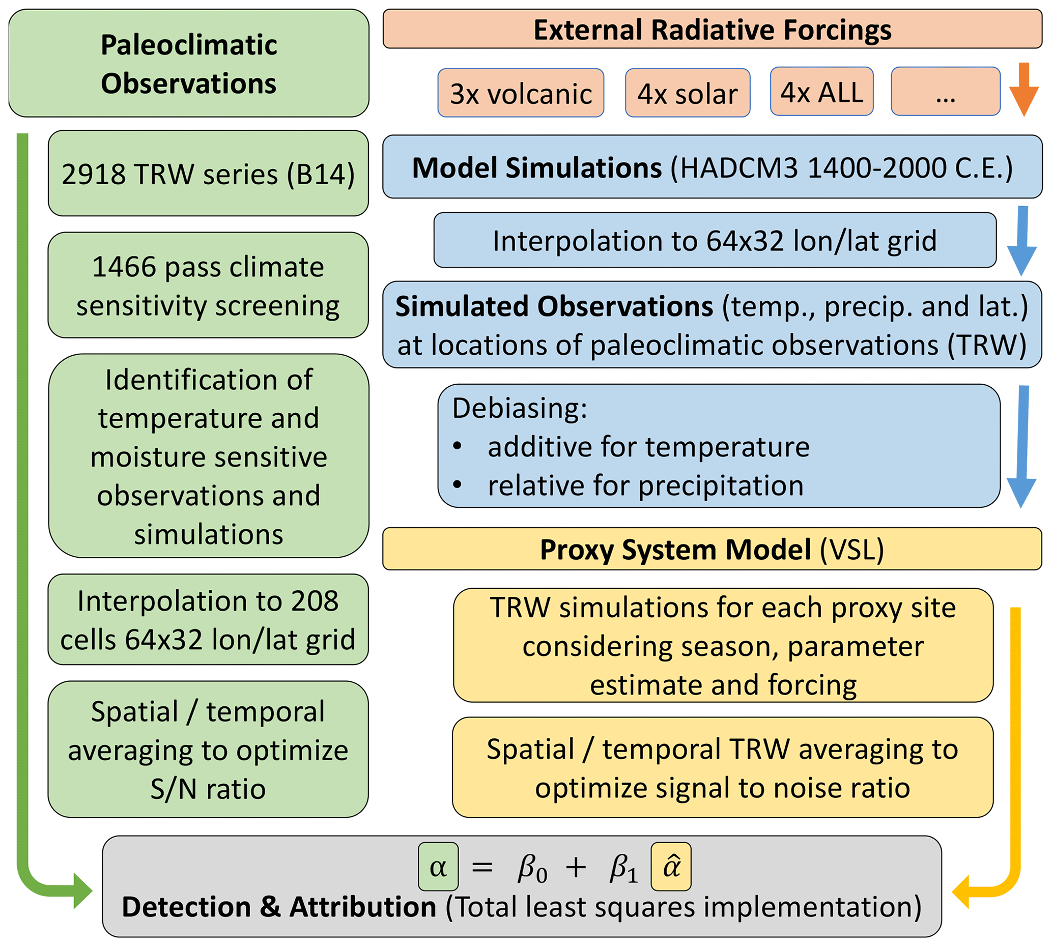
Figure 1 Schematic overview of the performed analysis. General steps are indicated in bold, and study-specific procedures are shown in roman text. B14 refers to the Breitenmoser et al. (2014) dataset, $S/N$ stands for signal to noise ratio, T stands for temperature and PREC stands for precipitation.

The remainder of this paper is organized as follows. First, we estimate and evaluate parameters for VSL, using gridded instrumental temperature (T) and precipitation (PREC) estimates and contemporaneous TRW observations (Sect. 2.2) in the period 1901–1970. Then VSL is used to build ensembles of simulated TRW series in response to singly and cumulatively forced simulations of T and PREC, given uncertainty propagated through the parameter estimation process and with bias corrections for simulated T and PREC ensembles (Sect. 2.3). We then estimate the D&A coefficients and their propagated uncertainty (Eq. 2; Sect. 2.4). The results are analyzed locally, regionally and globally for detection and attribution of a forced climate response, vis-à-vis the simulated and actual TRW observations (Sect. 3). We discuss the results and the potential to extend the approach in Sect. 4; conclusions are drawn in Sect. 5.

2 Data and methods

The inputs into and process of this detection and attribution study are illustrated in Fig. 1 and described below.

2.1 Tree-ring width measurements

We use the tree-ring width (TRW) collection described by and employed in Breitenmoser et al. (2014), now referred to as B14, as the observational basis for the development and validation of VSL parameters and as the D&A predictand (Eq. 1). B14 consists of 2918 uniformly detrended and standardized tree-ring width chronologies from six continents and 163 species that had been uploaded to the International Tree-Ring Data Bank (ITRDB, Zhao et al., 2019) up to 2014. These series have been quality controlled for metadata errors, repetitive measurements, incorrect units, decimal point errors and misplaced positions (Table S1 in Breitenmoser et al., 2014). Detrending for biological age trends and stand dynamics and standardization to dimensionless growth indices was done in a hierarchical approach. If possible, negative exponential curves and linear regression curves of any slope were fitted. In case both methods failed, “a smoothing spline was fit with a 50 % cut-off frequency at 75 % of each series length” (ARSTAN, Cook, 1985; Breitenmoser et al., 2014). Multiple measurements at the same site have been combined into robust means (Cook and Kairiukstis, 1990), which are variance adjusted for changing sample size through time (Osborn et al., 1997). For every point in time, which is explicitly resolved as one value per growing season each year, a chronology is based on at least eight samples. We use the auto-regressive standardized (Osborn et al., 1997; Frank et al., 2007) version of the available chronologies from B14. We require that the chronologies have at least 40 years observed within the period 1901–1970 (see Sect. 2.2 below).

We restrict subsequent analysis of simulations and the D&A exercise to the extratropical Northern Hemisphere continental areas, where the vast majority of TRW observations are located, with high concentrations in North America, Europe and northern Asia (Fig. 2). Record length varies from 100–600 years (Fig. 2). Series availability is generally greatest between the mid-19th century and the late 20th century (Fig. 3), and the longest records are equally distributed in longitude across the Northern Hemisphere boreal terrestrial latitudes (Fig. 2).

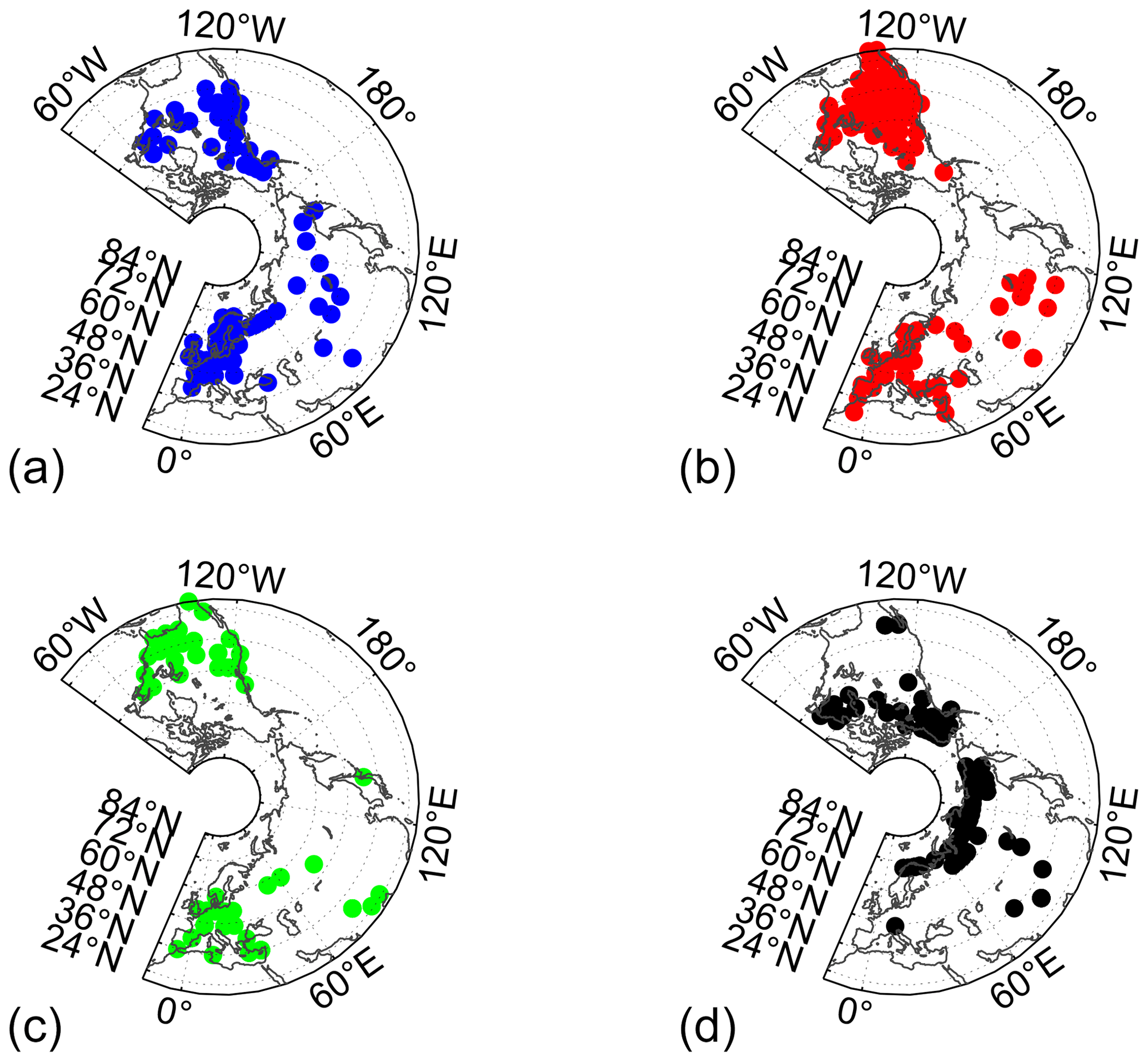
Figure 2 Limitations determined for all TRW chronologies with valid parameter sets, separated into temperature-sensitive values (a), moisture-sensitive values (b), both T- and M-sensitive values (c), and neither T- nor M-sensitive values (d). (Maps created with MATLAB mapping package M_map; Pawlowicz, 2022.)

2.2 VSL parameter estimation

For the purpose of VSL parameter estimation, we use the global, gridded instrumental temperature and precipitation datasets CRU TS 3.23 (Harris et al., 2014), regridded to 64 longitude × 32 latitude (∼5.6^∘) using a distance-weighted average of the four nearest-neighbor values. To correct for mean temperature biases, we applied an adiabatic (−6 K km⁻¹) T correction to the regridded CRU product, based on differences between elevations of grid points and elevations of observed TRW chronologies (Evans et al., 2006). Parameters T₁, T₂, M₁ and M₂ describe the onset of growth (1) and point above which climate is no longer a limiting factor (2) for temperature (T) and moisture (M), respectively (Tolwinski-Ward et al., 2011a, 2013). We conditioned and validated all four parameters simultaneously using contemporaneous observations and VSL simulations within the period 1901–1970. The growth period is defined as a 16-month interval. To integrate monthly incremental growth arising from pre-season and growing season, the growth integration period starts in September of the previous year and ends in December of the current year in the Northern Hemisphere (previous March to current June for the Southern Hemisphere), the same period as in Tolwinski-Ward et al. (2011a) and Breitenmoser et al. (2014). Other VSL parameters are not calibrated but taken from other studies (Evans et al., 2006; Fan and van den Dool, 2004; Huang et al., 1996; Tolwinski-Ward et al., 2011a, 2013; Vaganov et al., 2006; van den Dool, 2003). Within the chosen parameter estimation time window 1901–1970, with available N≥40, half of the years for which observed TRW data were available were chosen at random for parameter estimation (“calibration”, Tolwinski-Ward et al., 2013). The other half were reserved for validation of the estimated parameters via simulation using the estimated parameters; T and PREC are not used to estimate the parameters, and comparison with the TRW observations is withheld from the calibration process. The process was then repeated, now using the second half of data for parameter estimation (calibration) and the first half for validation of this parameter set. Up to 200 parameter sets were stored as valid if all four calibration and validation correlations between simulated and observed TRW were all independently significant at the p<0.1 level; all others failing this validation test were discarded.

2.3 VSL simulations, 1401–2000

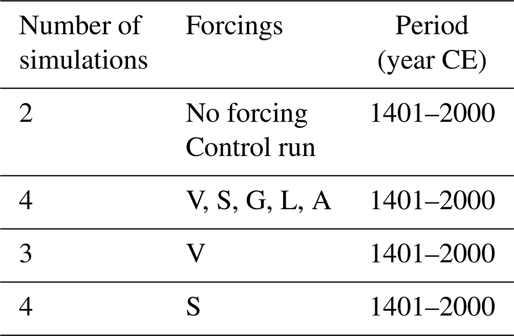
Temperature and precipitation input data for VSL are derived from climate model simulations. We use the set of simulations described in Schurer et al. (2014), which have been conducted with HADCM3 and interpolated to the same 64×32 grid as described in Sect. 2.2, to produce TRW simulations driven by singly and cumulatively forced climate simulations (Table 1). Because simulated T and PREC are spatially and seasonally biased relative to historical gridded T and PREC, we first correct the HadCM3 T and PREC fields for bias by computing T and PREC anomaly fields and adding them to (scaling them by) the CRU TS3.23 T climatology (PREC variability) for the overlapping period 1901–2000 CE. This step also ensures that systematic differences in mean simulated T and PREC will not systematically bias VSL simulations based on parameter estimates conditioned on the historical CRU TS3.23 T and PREC products. Using the methodology as described in Tolwinski-Ward et al. (2013, their Fig. 8), we then identified the primary limiting factor for simulated growth (at p<0.05, assuming a binomial distribution) and divided the simulated chronologies into TRW simulations that are primarily temperature limited, primarily moisture limited (M), limited by both or limited by neither. The median values, over parameter estimate realizations, of T- and M-sensitive TRW simulations were then separately weighted by inverse distance between observed and simulated grid points, observed expressed population signal (EPS, Wigley et al., 1984), and observed mean correlation between increment series within a chronology (RBAR, Cook and Kairiukstis, 1990) and averaged. Observed TRW were gridded and averaged in the same way as described above for subsequent D&A analysis (see Fig. 1 for a schematic overview of the entire process chain). Because centennial-scale climate variability may not be consistently preserved in the TRW records (Cook et al., 1995; Franke et al., 2013), and these timescales are poorly sampled in the 600-year period available for study, we removed low-frequency variability by applying a 71-year high-pass LOESS filter to both observed and simulated gridded TRW and focus our analyses on this residual interannual to multidecadal variance at annual resolution. The choice of annual resolution reflects the observational resolution (Sect. 2.1), the time-integrating nature of the sensor model (Sect. 2.2), the uncertainty of implementing radiative forcing estimates in the climate simulations (Gao et al., 2008),and the response timescale of the climate system to the large-scale forcing. We call the results, on which we base the detection and attribution analyses, climate-sensor simulations. This nomenclature reflects modeling of both the climate in response to external radiative forcing(s) and the tree-ring width observation that is the basis for the comparison with actual TRW observations.

Table 1 All-forcing and single-forcing HADCM3 simulations and control runs used in this study (“V” stands for volcanic, “S” stands for solar, “G” greenhouse gases, “L” stands for land use, and “A” stands for tropospheric aerosols).

2.4 Detection and attribution

To solve for the D&A coefficients in Eq. (1), we use the total least-squares (TLS) D&A technique to account for errors in both dependent and independent variables within the regression procedure (Allen and Stott, 2003) to account for internal variability in both observations and model simulations. We follow the analysis used in Allen and Stott (2003), Polson et al. (2013a), and Schurer et al. (2013), which estimates a best-fit regression coefficient (β) given by the following equation:

$$\begin{array}{}\text{(2)}& \mathit{\alpha }=\mathit{\beta }\left(\widehat{\mathit{\alpha }}-\mathit{\nu }\right)+\mathit{\nu }.\end{array}$$

In this study, $\widehat{\mathit{\alpha }}$ represents the simulated tree-ring widths and α represents the observed tree-ring widths, either at each grid box or spatially and/or temporally aggregated to increase the signal to noise ratio. ν represents the realizations of internal variability. Confidence intervals are obtained with the bootstrap method described in DelSole et al. (2019). They are calculated by randomly sampling (with replacements) pairs of values from the arrays of observed and simulated tree-ring widths to form new arrays that are the same length as the originals. A new scaling factor is then calculated by regressing the resampled model onto the resampled observations to represent uncertainty due to random noise. This process is repeated 10 000 times, and a 5 %–95 % confidence interval is estimated from the distribution. If the distribution of beta values is significantly greater than 0 (p<0.05), then the effect of the response to the forcing is considered to have been detected. If the distribution of β values is significantly less than unity,the response in climate-sensor simulations is significantly greater than observed, and the simulated climate sensitivity is smaller than observed. Conversely, if the scaling range is significantly greater than unity, the simulated climate-sensor response is significantly smaller than observed in TRW, and the climate sensitivity of the model may be inferred to be larger than observed.The estimate of the unforced variability as the residual of the D&A regression model provides another important result that needs to be compared with unforced variability of climate simulations (control runs) as a check of variability (PAGES 2k Consortium, 2019).

3 Results

3.1 Parameter estimation, TRW simulations and TRW observations

A total of 1664 of 2761 TRW chronologies in the B14 compilation were climate sensitive and therefore successfully simulated and retained for further analysis. With small differences between climate simulations, we found that 21 % of the successfully simulated chronologies are temperature sensitive, ca. 57 % are moisture sensitive, ca. 11 % are both moisture and temperature sensitive, and ca. 11 % are not climate sensitive, i.e., neither moisture nor temperature sensitive (Fig. 2). Distributions of temperature, moisture, both temperature and moisture, and neither temperature nor moisture sensitivity overlap in space. There are many moisture-sensitive TRW chronologies found in North America, the Mediterranean and other arid regions (Fig. 2b). However, there are also temperature-sensitive chronologies (Fig. 2a) and mixed responders (Fig. 2c) that are co-located in arid regions (Fig. 2a). Chronologies found to be neither temperature nor moisture sensitive (Fig. 2d) tend to be found at the highest latitudes, but this is not exclusively the case.

We found that bootstrapped VSL parameter estimates were in many cases distinctly non-normal in distribution for some or all of the four parameters and for some TRW simulations. Distributions were sometimes uniformly distributed across the prior expected parameter ranges, unimodal non-normal and even bimodal. Because there were not necessarily well-defined means or medians across parameter sets and simulations, we used all valid parameter sets to produce TRW simulations. Hence, we propagate uncertainty arising from stochastic variation in the climate simulations through parameter and structural uncertainty in the ring width sensor model.

Because the fingerprint of external radiative forcing may or may not be distinct and unique in temperature and moisture, we use the fit of VSL diagnostic variables G_T and G_M (estimate of nondimensional growth arising from temperature and soil moisture conditions, respectively) to binomial distributions to determine whether each simulation is primarily controlled by temperature, moisture, both or neither at the p<0.05 significance level (Tolwinski-Ward et al., 2013). We perform a similar analysis to determine the same primary growth controls in the TRW observations, using the same diagnostics from the parameter estimation exercise. We then average TRW observations to the simulation grid resolution for temperature- and moisture-limited simulations separately. Where there are multiple observed TRW chronologies available within a particular grid box, we construct a weighted average using inverse grid-point distance and intra-chronology mean incremental growth series correlation as weighting factors.

TRW simulations (Sect. 2.2, 2.3) are developed for all locations where TRW observations exist and the parameter estimation has been successful, i.e., for most of the extratropical Northern Hemisphere (Fig. 3). We exclude the Southern Hemisphere in this because only five temperature-sensitive chronologies and one moisture-sensitive chronology are located there. The record length of the simulations is constrained by TRW observations (see Sect. 2.1 and Fig. 3). The longest records are equally distributed in longitude across the Northern Hemisphere boreal terrestrial latitudes (Fig. 3). Thus, statistics assessed across the simulations and observations are best described as representing the Northern Hemisphere temperate and subpolar terrestrial regions.

Furthermore, we note that the locations of temperature- and moisture-sensitive chronologies overlap (Fig. 2) but are generally not coincident (Fig. 3): for either the observed or simulated sets, only about one-third are both coincident in space and significantly correlated with each other (Fig. 2). Hence, for the remainder of the analysis presented here, we develop and discuss the temperature- and moisture-sensitive results separately.

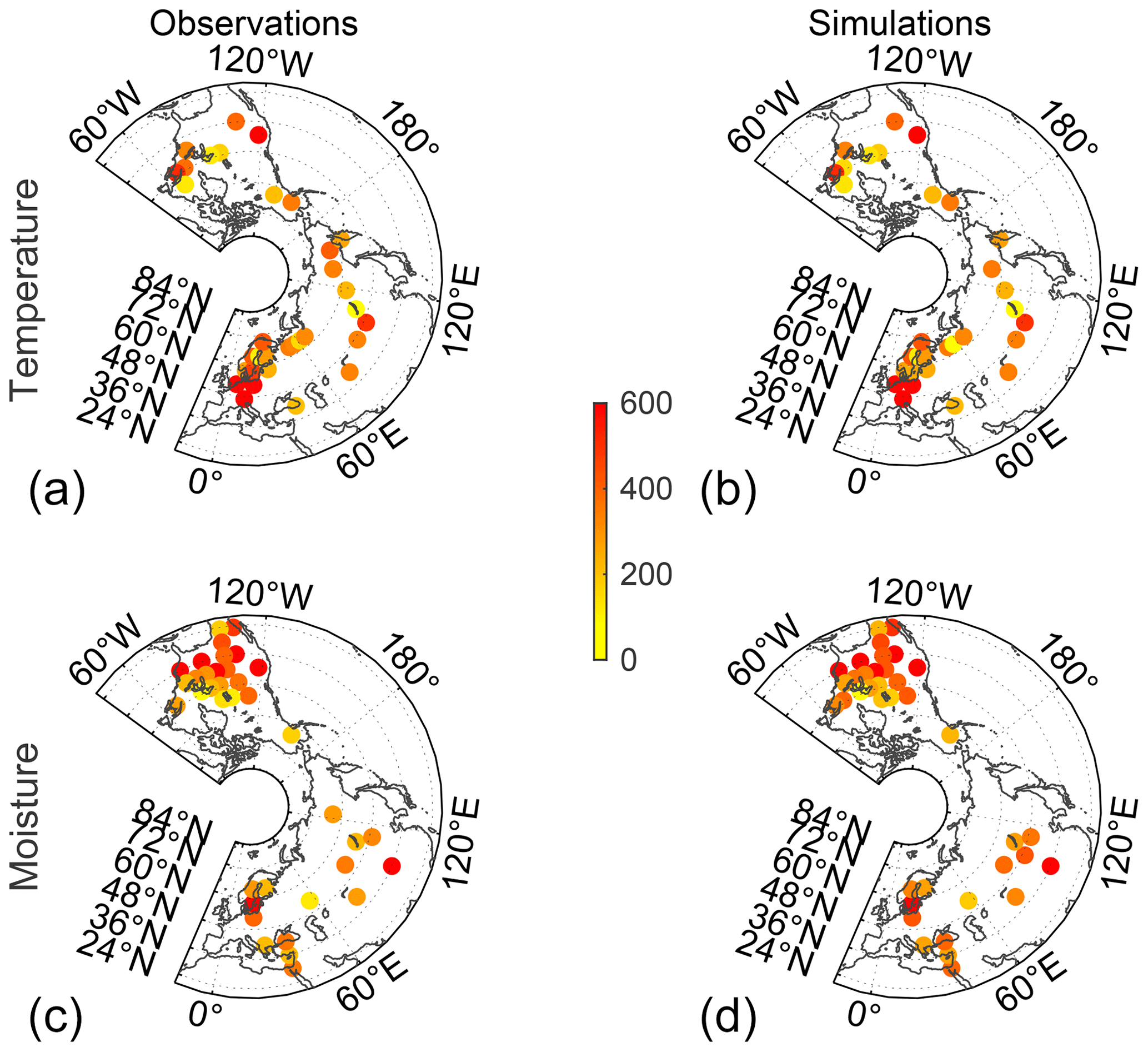
Figure 3 Numbers of years (color scale) available for comparison between gridded, observed and climate-sensor-simulated TRW chronologies, within the period 1401–2000. (a, c) Observed and (b, d) simulated temperature-sensitive chronologies. Simulated chronologies are masked by observational availability and in some cases (e.g., subpolar Eurasia) are neither moisture- nor temperature-sensitive or are both temperature and moisture sensitive and thus do not appear in either simulation map. Panels (c) and (d) are the same as panels (a) and (b) but for moisture-sensitive chronologies. (Maps created with MATLAB mapping package M_map; Pawlowicz, 2022.)

Figure 4 shows the growth functions G_T and G_M for the subsets of temperature- and moisture-sensitive identified TRW chronologies (Sect. 3.1). Although VSL has well-known limitations, for instance the lack of a soil moisture model allowing for snow, and despite the potential for an unrealistic and coarsely resolved annual cycle in the HadCM3 simulations, the results suggest plausible seasonality of the growth response of the TRW simulations. In particular, G_T for T-sensitive chronologies is maximum but limiting in June–October with a median response (black line) maximum for July–September. G_M for the T-sensitive subset of chronologies is not limiting through the same period. Similarly, for M-sensitive chronologies, G_M is limiting between July–December. G_E (the scaling associated with insolation (energy) as a function of latitude) is limiting (G_E <0.7) after September for latitudes poleward of 20^∘ N (results not shown), and G_T is not limiting through the warm months.

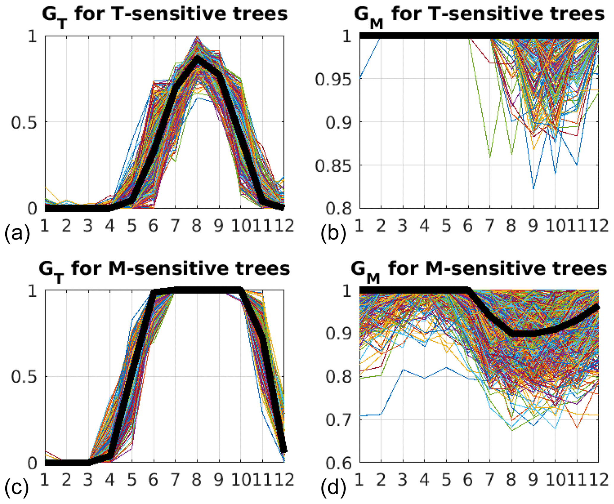
Figure 4 Simulated intra-year partial growth response functions G_T (a, c) and G_M (b, d) for T-sensitive (a, b) and M-sensitive (c, d) simulations using all climate simulations, with parameters conditioned and validated using observed TRW data within the period 1901–1970. Heavy solid lines are median values across all simulations.

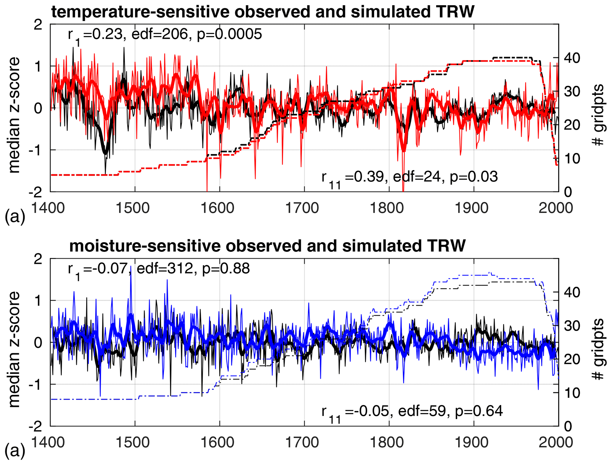
Figure 5 (a) Mean series for observed (black) and all-forcing-simulated temperature-sensitive chronologies (red). Annually resolved and a 11-year Hanning window filtered time series are shown with thin and bold lines, respectively. Labels quantify the Pearson correlation (r), effective degrees of freedom (edf, Hu et al., 2017) and the p value. The x axis is in units of years CE. (b) The same as (a) above but for moisture-sensitive observations (black) and simulations (blue). Note that this plot shows the global means of standardized TRW at all grid boxes with data before high-pass filtering and variance adjustment. There are small differences in numbers of observed and simulated chronologies that arise from both the observational masking and from the simulation parameter validation procedure (Sect. 2).

3.2 Comparison of observed and sensor-simulated TRW

To detect an external-forcing signal in noisy, local observations, the signal-to-noise ratio has to be enhanced. This is commonly achieved by averaging in space and/or time (Sects. 1, 2.4). We begin with analysis of global mean TRW variability at all locations where tree growth is either temperature or moisture limited, for comparisons between TRW observations and climate-sensor simulations driven with all forcings (Table 1). The variance of the average over all grid boxes increases back in time because of the decreasing numbers of records (Fig. 5), likely reflecting increasing uncertainty; the variance in the beginning of the 15th century is twice as large as that observed at the end of the 20th century. To reduce the sensitivity of the detection and attribution analysis to observational uncertainty, we homogenize the variance through time by multiplication of a time-dependent factor that is estimated by linear regression of the observed variance on the variance of TRW climate-sensor simulations from the control simulations.

Results suggest limited but significant correlation between global mean observed and simulated TRW temperature-sensitive simulations for both annual and decadally filtered series (Fig. 5). Nonsignificant correlations are found for moisture-sensitive observations vs. simulations at both annual and decadal timescales (Fig. 5). We find similar results for correlations between volcanically forced simulations and temperature-sensitive (r₁=0.22, edf =201, p=0.001; r₁₁=0.48, edf =19, p=0.02) and moisture-sensitive (r₁=0.01, edf =380, p=0.40; r₁₁=0.00, edf =54, p=0.51) observations. Correlations are not significant for comparisons between observed and solar-forced or unforced TRW simulations (results not shown).

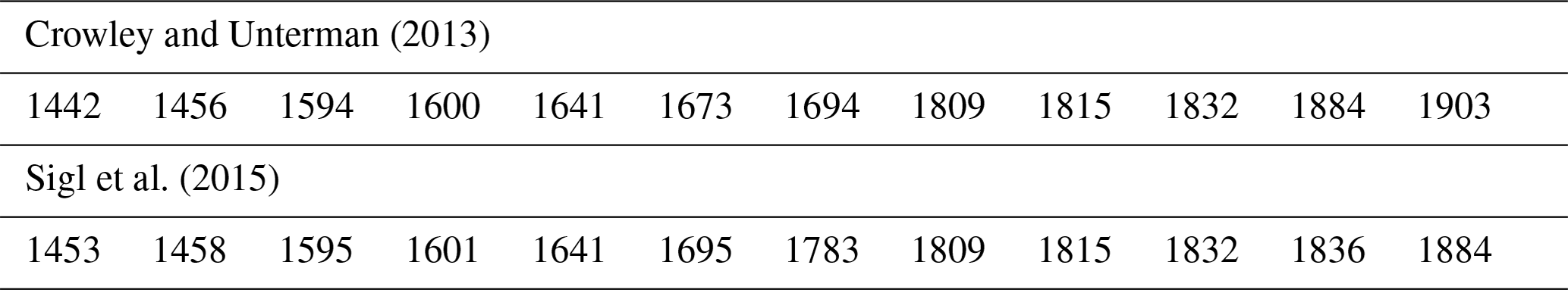
Based on these results, we test for detection of patterns in the TRW following volcanic eruptions in temperature- and moisture-sensitive TRW chronologies using a composite analysis across the seven largest (above 95th quantile) volcanic forcing responses for events between 1670 and 1970 (Fig. 6). We show the composite for observations based on two forcings, stratospheric atmospheric optical depth (AOD) reconstructed by Crowley and Unterman (2013) that was used to force the climate simulations (Fig. 1; Table 2) and the more recent and probably more realistic inferred global volcanic aerosol forcing (GVF, in W m⁻²) by Sigl et al. (2015). We do not use the full period back to 1401 because only a few locations have data reaching that far back in time. However, including up to 12 eruptions where available leads to a very similar pattern (not shown). Consistent with the results for observed averaged temperature-sensitive chronologies, we find a reduction in simulated tree growth in the first 2 years after the eruption in nearly all locations worldwide (Fig. 6, top right), with perhaps a more statistically significant cooling response in the Crowley and Unterman (2013) event chronology. Observed tree growth at the temperature-sensitive sites is reduced in most locations but not as homogenously as in the simulations (Fig. 6, top left). Possible reasons may be related to the small sample size, uncertainties in the reconstruction of the volcanic forcing (Sigl et al., 2015), a low climate signal-to-noise ratio in ring width, and an enhanced signal-to-noise ratio in the simulations, which are represented by their three-member ensemble mean (Table 1). Additionally, moisture influences may not be perfectly removed from the temperature-sensitive observations because some of the positive growth anomalies appear in locations for which tree growth tends to be generally moisture limited (in southwestern North America, northern European lowlands and the eastern Mediterranean; St. George and Ault, 2014) Thus, the composite observed temperature-sensitive response may in part also reflect increased moisture in dry regions following volcanic eruptions (Iles and Hegerl, 2015).

Table 2 Largest volcanic eruptions used in the composite analysis based on atmospheric optical depth (years CE).

For our moisture-sensitive comparison, we do not find a global volcanic response of the same sign but rather regions with uniform responses (Fig. 6, bottom row). The simulated event composite based on Crowley and Unterman (2013) (Fig. 6f) produces positive growth anomalies around the Mediterranean and in western North America and negative anomalies in Eurasia and eastern North America, with more prominent composite positive regions than negative regions. The observed composite based on the Toohey and Sigl (2017) chronology produces no negative composite response in eastern North America and a small positive response in southwestern North America, the latter of which is consistent with simulations (Fig. 6e and f).

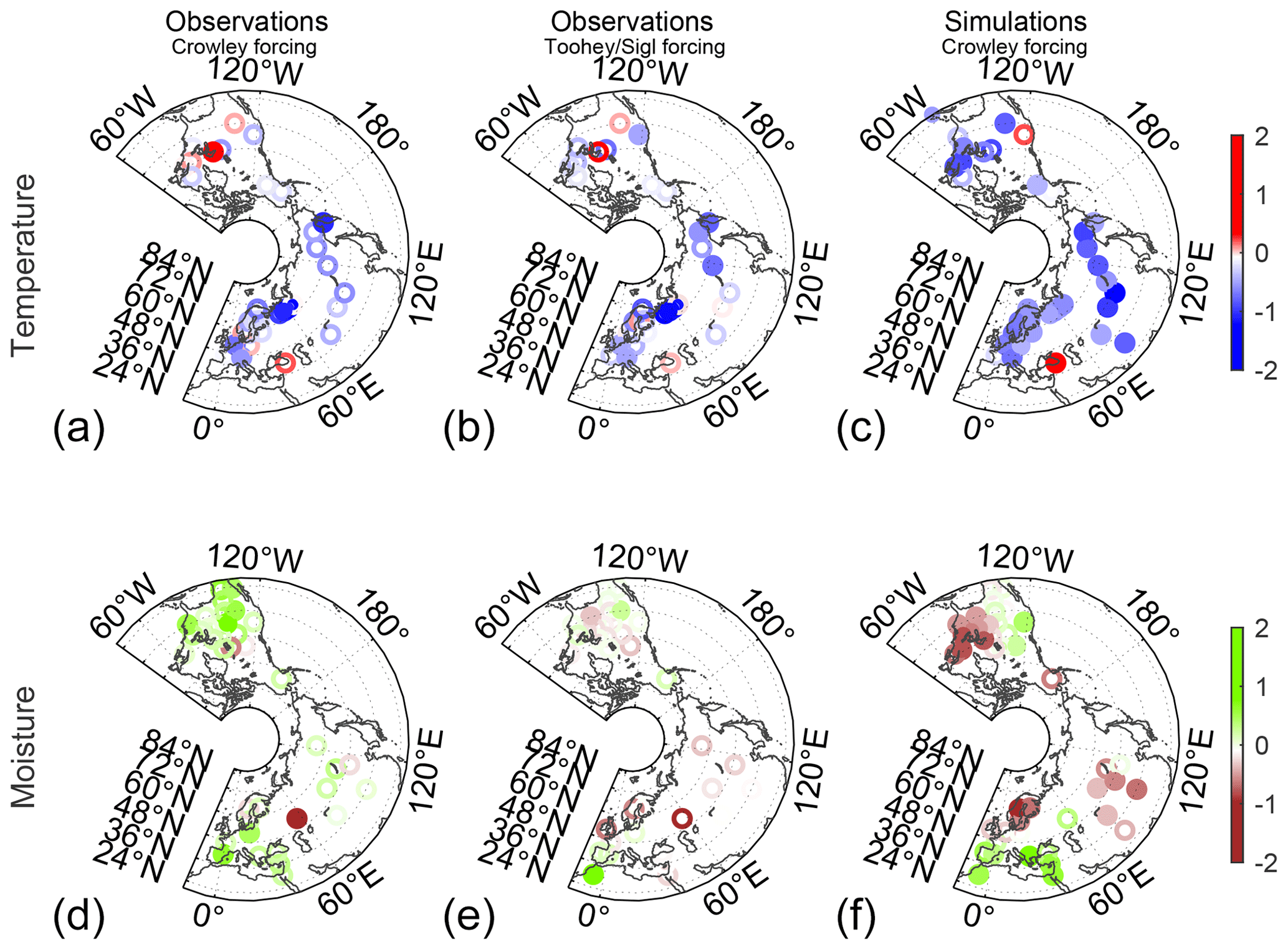
Figure 6 Composite average ring width anomaly (standardized units) in temperature-sensitive TRW chronologies in the first 2 years after volcanic eruptions in observations and volcanic-forcing simulations (a, b, c). Because relatively few TRW records are available for 1400–1700 (Fig. 2), the composite includes the seven strongest eruptions between 1670 and 1970 based on the eruption chronologies of Crowley et al. (2013) (a, d, c, f) and Sigl et al. (2015) (b, e). Panels (d), (e), (f) are the same as panels (a), (b), (c) but for moisture-sensitive TRW observations and simulations. Closed circles indicate statistical significance (p values of t test <0.05).

3.3 Detection and attribution analysis

We detect and attribute a response to volcanic forcing in both the spatial mean temperature time series and the spatiotemporal pattern of moisture-limited tree-ring records. As large volcanic eruptions disturb the climate system for a few years, we show results 3-year and 11-year moving averages. For the 3-year smoothed temperature-sensitive TRW averaged over all grid boxes, we find a significantly detectable scaling factor β that is not significantly different from 1; in other words, observed and simulated temperature-sensitive chronologies agree within uncertainty (Fig. 7a). This is true for both the all-forcing- and the volcanic-forcing-based TRW simulations (β_ALL and β_VOLC). For decadal averages (Fig. 7b), both scaling factors are likely greater than 1 and indicate that the observed responses are larger and/or more persistent than the simulated responses. Increased persistence is consistent with superposed epoch analysis results for volcanic eruptions using tree-ring data (see Lücke et al., 2019).

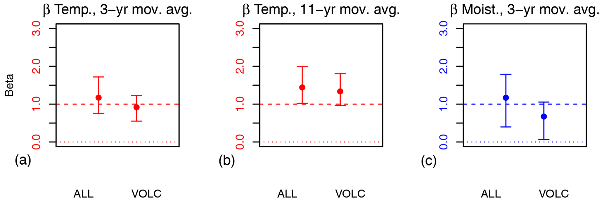
Figure 7 (a) Beta values and uncertainties for 3-year moving averages (following DelSole et al., 2019) in the TLS D&A analysis for temperature-sensitive TRW (Fig. 2a, b). ALL and VOLC indicate regression on the all-forcing- and volcanic-forcing-based TRW simulations, respectively. Panel (b) is the same as panel (a) but for 11-year running means; uncertainties are adjusted for serial autocorrelation. Panel (c) is the same as panel (a) but for moisture-sensitive TRW (Fig. 2c, d) with the aggregate mean response grouped by the two regions based on the positive or negative response of the TRW simulations (Fig. 6f). Uncertainty ranges are based on 90 % confidence intervals of scaling factors.

As described above, moisture-sensitive trees show positive growth anomalies in some regions and negative anomalies in other regions. We define a two-region spatiotemporal pattern identified in the moisture-sensitive TRW simulations (Fig. 6f). Scaling factors that are not significantly different from one for both all-forcing and volcanic-forcing simulations (Fig. 7c) again allow us to attribute moisture changes in response to volcanism.

4 Discussion

Detection and attribution studies using paleoclimatic data have previously focused on regression of reconstructed climate variables on realistically forced climate simulations (PAGES 2k Consortium, 2019; Schurer et al., 2014). In this study, we have attached a validated, realistically multivariate and nonlinear, intermediate-complexity proxy-sensor model (Evans et al., 2013; Tolwinski-Ward et al., 2013, 2015) to enable the D&A framework within the space of the paleoclimatic observation – in this study, tree-ring width chronologies. Because this particular sensor model is a scaled and time-integrated transformation of temperature and precipitation variations into a single diagnostic that is commonly observed across the terrestrial landscape, the potential for fingerprinting either distinct univariate or integrated plant-stress-like signatures of the different radiative forcings becomes possible. The approach also substitutes structural and parametric uncertainty in the sensor model for the uncertainty arising from inversion of multivariate paleoclimatic observations for univariate climatic reconstruction, and it thus provides a complementary assessment of the uncertainty that propagates into the D&A results.

We find that the global mean forced response in temperature-sensitive TRW chronologies is consistent with observations within the 1401–2000 period, a result that supports the prior work using global mean surface temperature reconstructions as a predictand (Hegerl et al., 2006, and references therein) and implicitly the use of temperature-sensitive TRW chronologies for producing those results. However, we also find that moisture- and temperature-sensitive chronologies (Fig. 3) form distinct subgroups in space (Fig. 2) and in temporal averages (Fig. 4). The fingerprint of climate forcing, as determined by comparison between all-series-averaged temperature- and moisture-sensitive observations and simulations is statistically significant in temperature (but not in moisture) for both all-forcing and volcanic-forcing simulations (Fig. 7).

For the attribution analysis targeting volcanic forcing (Figs. 6, 7), we find disagreement in the amplitude of the temperature-sensitive forcing as a function of timescale, with the observed annual, 3-year, and decadal timescale variance being smaller than, equal to, and greater than the simulated variance, respectively (Fig. 7a and b). One explanation would be that the simulated peak temperature response to volcanic forcing is unrealistically large. This has been observed for the HadCM3 climate model simulation in a previous study (Schurer et al., 2013). Volcanic forcings used to produce the climate simulations may also be oversimplified in time and/or space relative to actual forcing (Stevenson et al., 2017), or its timing may be incorrect (yielding suppressed amplitude in reconstructions). For many eruptions with an unknown date, the eruption was set to 1 January, and the AOD is entered into the model in four equal latitude bands only, proportional to the amount of sulfur in the Antarctic and Greenland ice cores (Crowley and Unterman, 2013). Because TRW simulations are a simplified representation of actual TRW variation, they neglect the observational uncertainty and the potential for superimposed and competing influences, such that the simulated TRW response to forcing may be relatively large. This is indeed the case; for either volcanic forcing or all forcing, simulated variance is about one-third larger than observed variance (results not shown).

A further explanation could be that autocorrelations in observed and simulated TRW are different. We find observed mean TRW autocorrelation to be about two-thirds larger than that of volcanic-forced simulations (results not shown). Consequently, we find the observed TRW variance at decadal resolution to be significantly greater than simulated TRW variance. This result suggests that (i) the observed response contains decadal timescale non-climatic variation not adequately removed by observational signal processing (Cook and Kairiukstis, 1990); (ii) mechanisms represented in the climate simulations are inadequate to represent slower response timescales of volcanic forcing (Miller et al., 2012); and (iii) mechanisms of forest response to volcanic forcing via soil moisture, air temperature, or insolation variations as represented in VSL, or a combination of all three factors, are insufficient to represent the observed lower-frequency response (Esper et al., 2015; Lücke et al., 2019)Ṗrevious studies found scaling factors to increase as more smoothing is applied (Schurer et al., 2013). However, they did not reach the point of a significantly larger response in observations than simulations.

Previous studies based on historical observations found that volcanic eruptions produced positive precipitation and streamflow anomalies in the Mediterranean and the southwestern United States, whereas negative anomalies were observed at high latitudes and in western North America, the Indian and the Southeast Asian region, and the tropics (Iles et al., 2013; Iles and Hegerl, 2015). This is in agreement with the CMIP5-simulated precipitation response (Fig. 1a in Iles and Hegerl, 2015), although the pattern in observed precipitation was very noisy and not clearly observed. In contrast, the response was identifiable in observed streamflow data, which cover a longer period and integrate the precipitation response. Reasons that the precipitation response could not be detected are likely to include the small number of eruptions in the instrumental period over which a composite was formed, combined with low signal-to-noise ratio for precipitation (Fig. 1a in Iles and Hegerl, 2015), and the complex precipitation response pattern with regions of increases and decreases, which is more difficult to detect (see also Polson et al., 2013b). We would obtain similarly non-detection and non-attribution levels were we to define regions manually (e.g., northern Europe vs. Mediterranean or western vs. eastern North America) or for a smaller integration over the years following an eruption. This finding is in agreement with Rao et al. (2017), who see the effect in tree-ring reconstructed drought severity index only in a very small region of northwestern Europe, southern Spain and northern Morocco, and with Fischer et al. (2007), who found increased precipitation in the Mediterranean and Scandinavia and decreased precipitation in northwestern and central Europe following volcanic eruptions, although not to a level that is statistically significant in many locations and which is accompanied by high uncertainty in the reconstructed precipitation response. For such small-scale regions, our TRW network is too sparse, our simulation grid too coarse and the time span of the TRW series is too limited to calculate robust composites. The present study respects some of these challenges by extending the analysis several centuries into the past (Table 1), integrating the forced response over time and space (Fig. 7), and forming the attribution model using the native observed variable rather than a reconstructed climatic variable (Sect. 1; Fig. 1). We find a similar pattern in moisture-sensitive TRW (Fig. 6). Simulations are most consistent with the expected pattern if the composite is based on the same forcing chronology as that used to drive the underlying HadCM3 simulations (Crowley and Unterman, 2013). The pattern in TRW observations agrees better with the more recent volcanic forcing chronology of Sigl et al. (2015). This suggests the latter forcing series reconstruction may be more consistent with the response as observed in TRW. However, the two forcing chronologies are similar enough that the two-region detection and attribution analysis (Fig. 7, right panel) produces the significant detection of both the all-forcing and volcanic-forcing TRW signals, within uncertainty of unity, lending support to the conclusions of Iles and Hegerl (2015).

5 Conclusion

We have estimated the contribution by all forcing and volcanic forcing to tree-ring data, based on a detection and attribution study using observed and modeled tree-ring width data directly for the exercise. We found that temperature- and moisture-sensitive TRW data contain different signatures of the forced climate response over the past 6 centuries. Specifically, we find that the signature of the all-forcing and volcanic-forcing response is most evident across the mean of all temperature-sensitive chronologies but not across the mean of all moisture-sensitive chronologies. The amplitude of the temperature-sensitive forced response is larger than expected from the model simulations in decadally filtered results, suggesting inaccuracies in the representation of forcing and/or responses on those timescales in observations, simulations or both sources of information. Additionally, we detect and attribute a previously identified spatial pattern in moisture-sensitive response to volcanic forcing at annual timescales, with a dipole drying and moistening pattern similar to the one previously identified by others within the historical time period and with direct moisture observations. In this study we demonstrate for the first time that climate change D&A can be conducted directly on paleoclimatic observations and their multivariate, nonlinear proxy system simulations, allowing for a much more reliable model evaluation than possible if using reconstructed climate variables. The results may realistically diverge from those obtained by D&A studies using univariate surface temperatures reconstructed from similar datasets because the underlying observations may in reality be multivariate nonlinear responders. Further studies could improve upon this proof of concept by incorporating stable isotopic observations in combination with isotope-enabled climate model simulations and by accessing a longer time interval for developing composite analyses, additional data types and a larger ensemble of realistically forced climate simulations.