the Creative Commons Attribution 4.0 License.
the Creative Commons Attribution 4.0 License.
 | 15 Nov 2022
Leeuwin Current dynamics over the last 60 kyr – relation to Australian ecosystem and Southern Ocean change
Dirk Nürnberg
Akintunde Kayode
Karl J. F. Meier
Cyrus Karas
The Leeuwin Current, flowing southward along the western coast of Australia, is an important conduit for the poleward heat transport and inter-ocean water exchange between the tropical and the subantarctic ocean areas. Its past development and its relationship to Southern Ocean change and Australian ecosystem response is, however, largely unknown. Here we reconstruct sea surface and thermocline temperatures and salinities from foraminiferal-based and stable oxygen isotopes from areas offshore of southwestern and southeastern Australia, reflecting the Leeuwin Current dynamics over the last 60 kyr. Their variability resembles the biomass burning development in Australasia from ∼60–20 ka BP, implying that climate-modulated changes related to the Leeuwin Current most likely affected Australian vegetational and fire regimes. Particularly during ∼60–43 ka BP, the warmest thermocline temperatures point to a strongly developed Leeuwin Current during Antarctic cool periods when the Antarctic Circumpolar Current (ACC) weakened. The pronounced centennial-scale variations in Leeuwin Current strength appear to be in line with the migrations of the Southern Hemisphere frontal system and are captured by prominent changes in the Australian megafauna biomass. We argue that the concerted action of a rapidly changing Leeuwin Current, the ecosystem response in Australia, and human interference since ∼50 BP enhanced the ecological stress on the Australian megafauna until its extinction at ∼43 ka BP. While being weakest during the Last Glacial Maximum (LGM), the deglacial Leeuwin Current intensified at times of poleward migrations of the Subtropical Front (STF). During the Holocene, the thermocline off southern Australia was considerably shallower compared to the short-term glacial and deglacial periods of Leeuwin Current intensification.
- Article
(5416 KB) - Full-text XML
-
Supplement
(3508 KB) - BibTeX
- EndNote


The southern margin of Australia is one of the world's largest latitude-parallel shelf and slope regions (James et al., 1994) and is affected by large boundary currents to the east (East Australian Current) and west (Leeuwin Current) that transport tropical ocean heat southward (e.g., Wijeratne et al., 2018; Fig. 1). Many studies highlighted the seasonal and interannual variability associated with these currents, but also the impact of the decadal El Niño–Southern Oscillation (ENSO) climate variability on the strength and transport variability of these currents (e.g., Feng et al., 2003; Holbrook et al., 2011; Wijeratne et al., 2018).
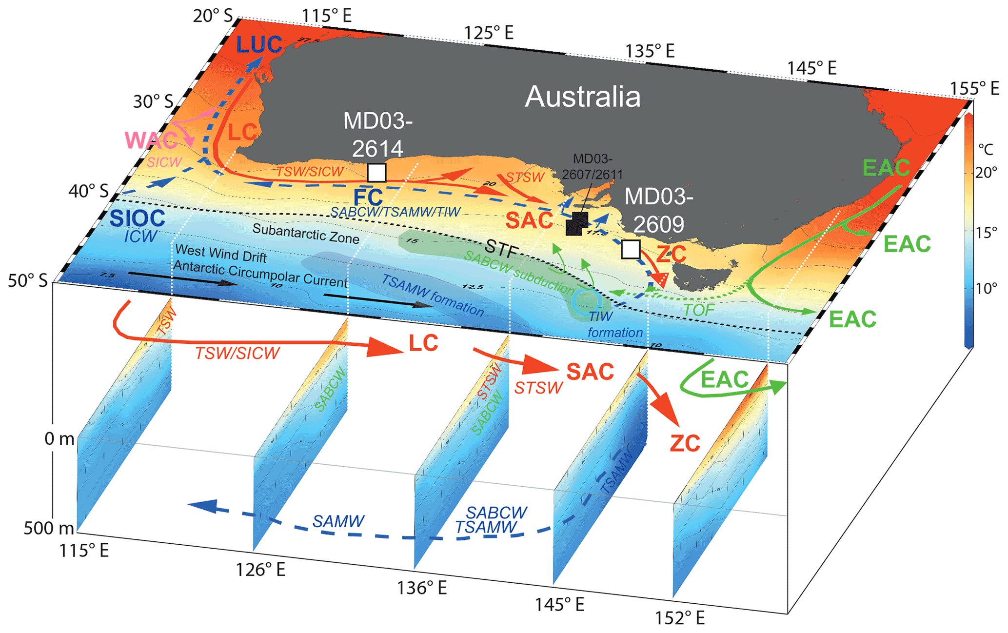
Figure 1The top of this image shows the regional surface and subsurface circulation pattern off southern Australia underlain by the modern annual SST pattern (using Ocean Data View v. 5.1.7; Schlitzer, 2019; World Ocean Atlas, Locarnini et al., 2019). Sediment core locations (MD03-2614 and -2609) studied here are marked by white squares. Black squares are reference sites. Surface currents are shown in red and green: LC is the Leeuwin Current, WAC is the West Australian Current, SIOC is the South Indian Ocean Current, SAC is the South Australian Current, ZC is the Zeehan Current, EAC is the East Australian Current, and TOF is the Tasman Outflow. Subsurface currents are shown in blue: FC is the Flinders Current, and LUC is the Leeuwin Undercurrent. Water masses transported by currents: TSW is Tropical Surface Water, ICW is Indian Central Water, SICW is South Indian Central Water, STSW is Subtropical Surface Water, SABCW is South Australian Basin Central Water, SAMW is Subantarctic Mode Water, TSAMW is Tasmanian Subantarctic Mode Water, and TIW is Tasmanian Intermediate Water. Sites of SABCW, TIW, and TSAMW formation are indicated. STF is the Subtropical Front (dashed black line). The bottom of the image shows the N–S-oriented temperature profiles (February) of the upper 500 m (dotted white lines; using Ocean Data View v. 5.1.7; Schlitzer, 2019). Currents, water masses, and sites of mode and intermediate water formation are from Richardson et al. (2019).
The warm and saline Leeuwin Current, an eastern boundary current that flows southward along the western coast of Australia (Fig. 1), originates from the Indonesian–Australian Basin and is fed by Indonesian Throughflow waters (ITW) and the eastward-directed Eastern Gyral Current (Meyers et al., 1995; Domingues et al., 2007). The Leeuwin Current turns east into the Great Australian Bight (Cresswell and Golding, 1980; Church et al., 1989; Smith et al., 1991) and shapes the temperature and salinity conditions and water column stratification off western and southern Australia (Legeckis and Cresswell, 1981; Herzfeld and Tomczak, 1997; Li et al., 1999; Middleton and Bye, 2007; Holbrook et al., 2012). Wells and Wells (1994) concluded from micropaleontological studies that the Leeuwin Current likely stopped flowing during glacial periods, while the northwest-directed West Australian Current (Fig. 1) gained strength, resulting in a large-scale reorganization of the regional circulation patterns. Martinez et al. (1999) reported on the reduced occurrence of tropical planktonic species in the eastern Indian Ocean during glacial periods, while abundances of intermediate and deep-dwelling species increased, which they related to a weakened Leeuwin Current. Spooner et al. (2011) argued instead that the Leeuwin Current remained active although weakened during the last five glacial periods, while the West Australian Current strengthened.
For the interglacial Marine Isotope Stages (MISs) 5, 7, and 11, Spooner et al. (2011) inferred a stronger Leeuwin Current due to an enhanced Indonesian Throughflow contribution. De Deckker et al. (2012) and Perner et al. (2018) attributed the alternating warm and cold phases in the Great Australian Bight to changes in both Leeuwin Current-related heat export from the Indo-Pacific Warm Pool and latitudinal shifts of the Subtropical Front (STF; Fig. 1). A study from off Tasmania (Nürnberg et al., 2004) already pointed to a STF, which was commonly located further to the south during interglacials, while its glacial position moved northward and allowed subantarctic waters to expand northward. Moros et al. (2009) suggested that the STF was located closer to the southern Australian coast during the early Holocene (∼10–7.5 ka BP) than its current position today at ∼45∘ S in winter.
Despite the many efforts to understand the paleoceanographic setting south of Australia (e.g., Wells and Wells, 1994; Findlay and Flores, 2000; Barrows and Juggins, 2005; Nürnberg and Groneveld, 2006; Calvo et al., 2007; Moros et al., 2009; Spooner et al., 2011; De Deckker et al., 2012; Lopes dos Santos, 2012; Perner et al., 2018), no proxy studies and only a few modeling studies have concentrated on the subsurface development (e.g., Schodlok and Tomczak, 1997; Middleton and Cirano, 2002; Middleton and Platov, 2003; Cirano and Middleton, 2004; Middleton and Bye, 2007; Pattiaratchi and Woo, 2009). The aim of our study is to fill this important gap and to reveal changes in the Leeuwin Current over the last 60 kyr. Stable oxygen isotope (δ18O), -based reconstructions of surface and thermocline temperatures (SST; TT, and regional ice-volume-corrected δ18O of seawater (δ18Osw-ivc approximating surface and thermocline salinity) from two sediment cores off southern Australia (MD03-2614 and MD03-2609) allow us to address the past dynamics of the vertical water column structure south of Australia in response to latitudinal shifts of oceanographic and atmospheric frontal systems and the impact of the Southern Ocean change in the study area.
2.1 Currents and winds
The Leeuwin Current and the Flinders Current are the main two current systems affecting the ocean region south of Australia (Fig. 1). The East Australian Current, a strong western boundary current (>2 m s−1) transporting tropical heat poleward along eastern Australia, only sporadically affects the southern coast (Bostock et al., 2006). The Leeuwin Current flows southwards along the western Australian shelf break and is characterized as a shallow (upper ∼200 m) coastal current, with low-salinity and nutrient-depleted waters that originate mainly from the Indo-Pacific Warm Pool. It receives further contributions of subtropical waters from the Indian Ocean via the broad equatorward-flowing West Australian Current, which is the eastern branch of the Indian Ocean gyre (Wandres, 2018).
After passing Cape Leeuwin and reaching its highest velocities, the Leeuwin Current turns east into the Great Australian Bight as far as ∼124∘ E (Ridgway and Condie, 2004). At the same time, it becomes saltier, cooler, and denser due to air–sea interactions, subtropical addition, and eddy mixing with Indian Ocean and Southern Ocean waters (see Richardson et al., 2019). Seasonal variations in the Leeuwin Current strength (Ridgway and Condie, 2004; Cirano and Middleton, 2004) reveal that the Leeuwin Current is strongest near the shelf edge in austral winter (June–July), with a maximum poleward geostrophic transport of ∼5 Sv (106 m3 s−1), and weakest in austral summer, with a mean transport of ∼2 Sv (Holloway and Nye, 1985; Rochford, 1986; Feng et al., 2003; Ridgway and Condie, 2004).
Cirano and Middleton (2004) estimated that the contribution of the Leeuwin Current on the total flow along the southern Australian coast diminishes toward the east. Off the eastern Great Australian Bight, the Leeuwin Current only drives ∼15 % of the total flow, while wind forcing (∼47 %) and a pressure gradient term (∼38 %) become more important. Ridgway and Condie (2004) noted that along the western Australian coast, the Leeuwin Current is forced by the alongshore pressure gradient associated with the meridional portion of either less dense and low-salinity water masses from the equatorial Western Pacific Warm Pool or southern-sourced cold, dense, and high-salinity waters, which exceed the equatorward alongshore winds. Along the southern Australian coast, the zonal shelf edge flow is instead forced by the austral winter westerly wind. Ridgway and Condie (2004) suggested that the western coast pressure gradient delivers the Leeuwin Current to the southern coast just in time for the (south)westerly winds to strengthen, thereby maintaining the eastward passage of the current.
The changing atmospheric circulation pattern is closely connected to the Subtropical Ridge, a belt of high-pressure systems (anticyclones) between ∼30 and ∼40∘ S (e.g., Drosdowsky, 2005), which divides the tropical southeasterly circulation (trade winds) from the mid-latitude westerlies. The Subtropical Ridge is shaped by the Indian Ocean Dipole, Southern Annual Mode (which is the zonal mean atmospheric pressure difference between the mid-latitudes (∼40∘ S) and Antarctica (∼65∘ S); Marshall, 2003), and to a lesser degree by ENSO (Cai et al., 2011). During austral autumn/winter (austral spring/summer), it moves north (south), allowing the westerlies to seasonally strengthen (weaken) rainfall in SE Australia (Cai et al., 2011). During El Niño conditions, the Subtropical Ridge is displaced farther equatorward than normal, while during La Niña conditions it is shifted poleward (Drosdowsky, 2003).
Near the eastern edge of the shallow Great Australian Bight shelf, a gravity outflow of warm and high-salinity waters related to intensified surface heating during austral summer spreads across the shelf and continues to flow eastward as the shelf edge South Australian Current (Ridgway and Condie, 2004; Fig. 1). Although relying on different forcing mechanisms, the South Australian Current is widely regarded as the extension of the Leeuwin Current. In the Bass Strait, the Leeuwin Current–South Australian Current system continues south as high-saline and relatively warm Zeehan Current (Ridgway and Condie, 2004; Richardson et al., 2018). South of Australia, the Leeuwin Current System meets the northern boundary of the eastward flowing Antarctic Circumpolar Current (ACC). Below, the deeper (300–400 m) equatorward flow of the Leeuwin Undercurrent is noted (Spooner et al., 2011). During austral summer, when the Leeuwin Current is weak, the equatorward Capes Current establishes at the inner shelf around Cape Leeuwin. Its formation is related to regional upwelling, bringing water masses from the Flinders Current and the lower layers of the Leeuwin Current towards the upper shelf areas (see McClatchie et al., 2006).
The westward-directed Flinders Current is a subsurface northern boundary current along the continental slope of southern Australia (Middleton and Cirano, 2002; Cirano and Middleton, 2004; Fig. 1). Maximum transport is at ∼400–800 m, with velocities of up to 8 cm s−1 (Middleton and Bye, 2007). It originates within the Subantarctic Zone and carries Subantarctic Mode Water (SAMW) and Antarctic Intermediate Water (AAIW) across the STF (McCartney and Donohue, 2007). Southeast of Australia, the Flinders Current is fed and strengthened by the Tasman Outflow, a remnant of the East Australian Current, which injects Pacific waters into the South Australian Basin (Rintoul and Sokolov, 2001) and becomes an important component of the westward flow south of Australia (Speich et al., 2002). The Flinders Current fluctuates in strength on a seasonal timescale (Richardson et al., 2019), with almost doubled transport (∼17 Sv) during austral summer compared to winter (∼8 Sv).
The Leeuwin Undercurrent, which is beneath the Leeuwin Current at depths of ∼250–600 m, transports ∼5 Sv of saline (>35.8 psu), oxygen-rich, and nutrient-depleted waters northward as an extension of the Flinders Current (Fig. 1; Thompson, 1984; Smith et al., 1991; Cirano and Middleton; 2004). Both currents are associated with SAMW (Pattiaratchi and Woo, 2009).
2.2 Water masses and oceanographic fronts
We here address three water masses within the uppermost 600 m along the continental slope of southern Australia (Figs. 1 and 2): Subtropical Surface Water (STSW), South Australian Basin Central Water (SABCW), and SAMW. The subtropical warm and saline STSW originates within the surface mixed layer (upper ∼200 m) along Australia's southern margin between 34 and 38∘ S as a result of surface heating and enhanced evaporation (James and Bone, 2011; Fig. 2). STSW constitutes the shallowest water mass along the southern Australian margin and is defined by temperatures >12 ∘C and salinities >35.1 (Richardson et al., 2018). The dissolved oxygen concentration is high (225–250 µmol L−1) and nutrients are low (Richardson et al., 2018). The water mass is additionally fed by low-salinity Tropical Surface Water (TSW) and high-salinity South Indian Central Water (SICW) contributed by the West Australian Current and the South Indian Ocean Current (Cresswell and Peterson, 1993). The maximum depth of the STSW is seasonally dependent: during austral autumn and winter, the Leeuwin Current-transported STSW is thicker (∼300 m in the western and ∼200–250 m in the eastern study area; Richardson et al., 2019) with a rather low vertical temperature gradient in the west (Fig. 2). When the eastward wind stress is strongest and opposing winds cease, it reaches further to the east and may reach the southern tip of Tasmania due to a strong Zeehan Current adjoining the Leeuwin Current (Cresswell, 2000; Feng et al., 2003; Ridgway and Condie, 2004; Ridgway, 2007), which causes warming at depth. During austral summer (November to March), the STSW remains west of ∼140∘ E (Newell, 1961; Vaux and Olsen, 1961; Ridgway, 2007; Richardson et al., 2018). It then is at shallower depths (∼200–250 m in the west and ∼150–50 m in the east; Richardson et al., 2019; Fig. 2), with a well-defined shallow thermocline during times of a weak Leeuwin Current, when opposing winds (blowing from the southwest) are strong (Godfrey and Ridgeway, 1985; Smith et al., 1991; Feng et al., 2003, 2009).
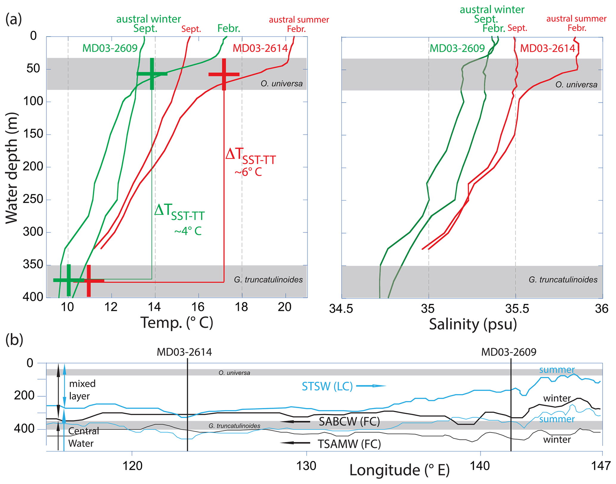
Figure 2Upper ocean hydrological setting south of Australia: (a) temperature (left) and salinity (right) distribution in the upper 400 m at the western core 2614 location (red) and at the eastern core 2609 location (green; cf. Fig. 1). Only maximum (February; austral summer) and minimum (September; austral winter/spring) temperatures and salinities are indicated. Presumed calcification depths of foraminiferal species analyzed are indicated by grey shading: O. universa at ∼30–80 m water depth (Anand et al., 2003; Farmer et al., 2007) and G. truncatulinoides at ∼350–400 m water depth (Cléroux et al., 2008; Anand et al., 2003). Modern average temperatures (crosses) and temperature gradients between surface and thermocline are indicated for the respective study areas. Data from Ocean Data View v. 5.1.7 (ODV Station labels 12796 and 11161; Schlitzer, 2019; WOA; Locarnini et al., 2019). (b) Average summer (blue) and winter (black) boundaries between the surface mixed layer (consisting predominantly of STSW, transported eastward by the Leeuwin Current, LC) and the Central Water (composed of SABCW and TSAMW, transported westward by the Flinders Current, FC), taken from Richardson et al., 2019). Core locations (vertical black lines) and assumed calcification depths of foraminiferal species studied are indicated.
The SABCW, showing a small range in potential density (26.65–26.8 kg m−3), is below the surface mixed layer (Fig. 2b). SABCW is defined by temperatures and salinities of 10–12 ∘C and 34.8–35.1, with a weak dissolved oxygen maximum (>250 µmol L−1; Richardson et al., 2018). Towards the east, the thickness of the SABCW is ∼200 m, while it decreases to ∼100 m in the west (Richardson et al., 2018). The thinning of SABCW towards the west is likely attributed to the presence of near-surface subtropical water in the west (STSW), contributed by the strong eastward-flowing Leeuwin Current. SABCW likely forms south of the STF between 44–46∘ S and 140–145∘ E in winter by convective overturning and subduction of the deep mixed layer (Richardson et al., 2018). The subducted SABCW reaches slope depths of ∼300–500 m at 142∘ E and ∼300–400 m at 130 to 121∘ E. It is transported eastwards towards Tasmania along the STF by zonal flow. The Flinders Current inflow from the southeastern margin then carries SABCW north and west, augmented by the Tasman Outflow and equatorward Sverdrup transport (Schodlok and Tomczak, 1997). Along the southern Australian margin, the boundary between the top surface of SABCW (as part of the Central Water) and the overlying STSW defines the interface between the eastward-directed Leeuwin Current System transporting subtropical waters and the westward flow of the Flinders Current System, which brings subantarctic waters into the region (SABCW coupled to Tasmanian Subantarctic Mode Water (TSAMW) and Tasmanian Intermediate Water (TIW); Fig. 2b; Richardson et al., 2019).
The coldest and densest SAMW of the Indian Ocean forms by air–sea interaction and deep winter mixing south of Australia between 40 and 50∘ S (e.g., Wyrtki, 1973; McCartney, 1977; Karstensen and Quadfasel, 2002; Barker, 2004). SAMW is subducted, thereby ventilating the lower thermocline of the Southern Hemisphere subtropical gyres (McCartney et al., 1977; Sprintall and Tomzcak, 1993). The high-nutrient SAMW is defined as a layer of relatively constant density (pycnostad) along the southern Australian continental slope (Richardson et al., 2019; Fig. 2). The pycnostad is clearly defined in the east, notably in summer, but diminishes towards the west (Richardson et al., 2018). The SAMW in this region is located at ∼400–650 m, with temperatures of ∼8–10 ∘C and salinities of 34.6–34.8 (Woo and Pattiaratchi, 2008; Pattiaratchi and Woo, 2009), being therefore fresher than the overlying SABCW and STSW. The top SAMW depth varies seasonally from west to east, as it shallows to ∼350 m during summer and deepens to ∼500 m in winter (Rintoul and Bullister, 1999; Rintoul and England, 2002). In particular, the Tasmanian SAMW (TSAMW) is formed in a clearly defined area at 45–50∘ S and 140–145∘ E (Barker, 2004).
In the framework of the International Marine Global Change Study (IMAGES), Calypso giant piston cores MD03-2614G (termed western core 2614; S, E; 1070 m water depth; 8.4 m core recovery) and MD03-2609 (termed eastern core 2609; S, E; 2056 m water depth; 24.18 m core recovery) were recovered south of Australia, ∼100 km south of Cape Pasley and ∼250 km northwest of King Island, respectively, during the AUSCAN campaign with RV Marion Dufresne (MD131) in 2003 (Michel et al., 2003). The chronostratigraphy of core 2614 was published by van der Kaars et al. (2017) and is repeated here, as core 2614 served as reference for the establishment of the core 2609 chronostratigraphy. The age model of core 2609 was established in the framework of this study.
3.1 Foraminiferal species selection
The chronostratigraphy and the paleo-reconstructions were established from isotope-geochemical parameters measured within the calcitic tests of the subtropical shallow-dwelling planktonic foraminiferal species Orbulina universa (Bé and Tolderlund, 1971) and Globigerinoides ruber and the deep-dwelling species Globorotalia truncatulinoides (Lohmann and Schweitzer, 1990). As O. universa preferentially lives in the surface mixed layer and the shallow thermocline, we assigned a calcification depth of ∼30–80 m (see Text S1 in the Supplement). The surface-dwelling G. ruber is the most representative species of warm and annual surface (<50 m) ocean conditions (Anand et al., 2003; Tedesco and Thunell, 2003). For G. truncatulinoides we assume a calcification depth of ∼350–400 m (see Text S1), which corresponds to the base of the summer thermocline (Fig. 2; Locarnini et al., 2019). Most of the G. truncatulinoides specimens in our samples were encrusted (see Text S1).
On average, 10–12 and 30–40 visually clean specimens of O. universa/G. ruber and G. truncatulinoides, respectively, were hand-picked under a binocular microscope from the narrow >315–400 µm size fraction in order to avoid size-related effects on either or stable isotopes. G. truncatulinoides has no size effect on (Friedrich et al., 2012), and δ13C and δ18O also show no systematic changes in the selected size fraction (Elderfield et al., 2002). The foraminiferal tests were gently crushed between cleaned glass plates to open the test chambers for efficient cleaning. Over-crushing was avoided to prevent an excessive sample loss during the cleaning procedure. The fragments of the tests were homogenized and split into subsamples for stable isotope (one-third) and trace metal analyses (two-thirds) and transferred into cleaned vials. Chamber fillings (e.g., pyrite, clay) and other contaminant phases (e.g., conglomerates of metal oxides) were thoroughly removed before chemical cleaning and analyses.
3.2 Chronostratigraphy
3.2.1 Western core 2614
The age model of the western core 2614 (Cape Pasley) is based on the linear interpolation between 11 accelerator mass spectrometry (AMS) radiocarbon (14C) dates (van der Kaars et al., 2017; Fig. 3). The well-constrained age model indicates that core 2614 provides a continuous record over the last ∼60 kyr (Fig. 3). In addition to the δ18O record of G. ruber (van der Kaars et al., 2017), we produced δ18O records of O. universa and G. truncatulinoides. Interesting to note is that a significant and rapid transition to heavy δ18O values in (only) O. universa from core 2614 is synchronous to a major atmospheric methane (CH4) anomaly detected in the Antarctic EPICA Dronning Maud Land (EDML) ice core record (EPICA Community Members, 2006), further supporting the validity of the initial core 2614 age model (Fig. 3).
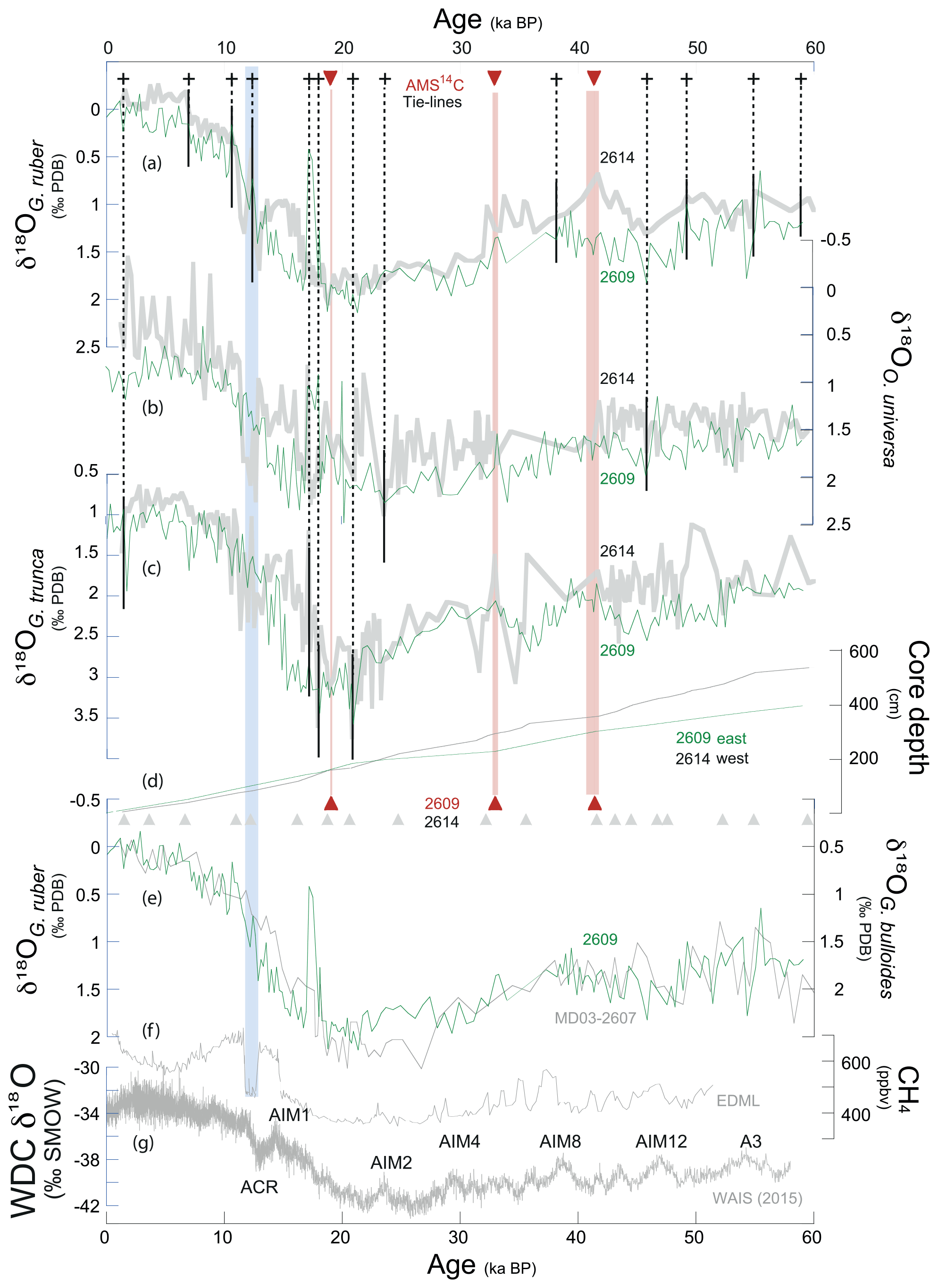
Figure 3Chronostratigraphy of the eastern core 2609 (King Island). The age model is based on the tuning of various planktonic δ18O records of (a) G. ruber, (b) O. universa, and (c) G. truncatulinoides (all in green lines) to similar records (thick grey lines) of the well-dated reference core 2614 (van der Kaars et al., 2017). In total, 13 tuning tie lines (stippled lines; solid for the species-specific correlations) were set in order to achieve an optimal fit of the core 2609 and core 2614 δ18O records (mean r2=0.86). The age model for core 2609 is supported by three AMS14C datings (red triangles and red lines; red shading marks the 1-sigma errors). (d) Sedimentation rates (green = core 2609; grey = core 2614). Grey triangles are age control points established for core 2614 by van der Kaars et al. (2017). (e) The age model for core 2609 is supported by the match of its δ18OG. ruber record (green) to the adjacent core MD03-2607 δ18OG. bulloides record (grey; Lopes dos Santos et al., 2013). (f) Atmospheric CH4 record from EPICA ice core (EPICA Community Members, 2006). Blue shading denotes prominent atmospheric CH4 anomaly synchronous to a distinct reflection in the core 2614 δ18OO. universa record. (g) West Antarctic Ice Sheet Divide Core δ18O record (WAIS Divide Project Members, 2015) as reference for the Southern Hemisphere climate signal.
3.2.2 Eastern core 2609
The age model of the eastern core 2609 is based on the tuning of multiple planktonic δ18O records to those of the well-dated reference core 2614 (van der Kaars et al., 2017) using the software AnalySeries (Paillard et al., 1996). For both cores, we produced δ18O records on G. ruber, O. universa, and G. truncatulinoides, all of which have either different spatial resolutions or even gaps (due to missing species), which are covered by one species or another (Fig. 3; https://www.pangaea.de/, last access: 11 November 2022). In a first step, we graphically tuned the δ18OG. ruber record of the eastern core 2609 to that of the western core 2614 (van der Kaars et al., 2017), thereby generating seven tuning tie-lines (Fig. 3a). This correlation was improved in a second step by tying the δ18OO. universa records of both cores to each other using two additional tie lines (Fig. 3b). In a last step, we correlated the δ18OG. truncatulinoides records of both cores, fixing them with four additional tie lines (Fig. 3c). Overall, we achieved an optimized fit of the core 2609 δ18O records to the core 2614G reference record (linear correlation =0.86, averaged from all δ18O records), by applying 13 tuning tie lines. The core 2609 age model is supported by three radiocarbon (AMS14C) datings (Fig. 3; see Text S1 and Table S3 in the Supplement), for which a mix of shallow-dwelling planktonic foraminiferal tests was selected. The measurements were accomplished by Beta Analytic, Inc., Florida, USA (info@betalabservices.com). All AMS14C dates were calibrated applying the BetaCal4.20 software using the MARINE20 database. The marine calibration incorporates a time-dependent global ocean reservoir correction of ∼550 14C yrs at 200 cal yr BP to ∼410 14C yrs at 0 cal yr BP (Heaton et al., 2020).
To account for local effects, the difference ΔR in reservoir age of the study area south of Australia and the model ocean was additionally considered. The Calib7.1 marine reservoir correction database provides a ΔR value of years (Stuiver and Reimer, 1993).
The resulting age–depth relationship of core 2609 is rather smooth, with a subtle change in sedimentation rates at 200–230 cm core depth. The age model implies that the uppermost ∼4 m of core 2609 capture the last 60 kyr of environmental change (Fig. 3). Our stratigraphical approach for core 2609 is convincingly supported by the match of the δ18OG. ruber record to the δ18OG. bulloides record of the adjacent core MD03-2607 from Murray Canyon ( S, E, 865 m water depth; Lopes dos Santos et al., 2013; Fig. 3e). The sedimentation rates in both cores 2609 and 2614 vary from 5 to 20 cm kyr−1 over the last 60 kyr (Fig. 3d), with persistently higher rates and higher-amplitude changes in the western core 2614 most of the time. Sampling of cores 2614 and 2609 was accomplished every 2 cm, providing a temporal resolution of on average ∼230 years for core 2614 and ∼290 years for core 2609.
3.3 Foraminiferal paleothermometry
Prior to elemental analysis, the foraminiferal samples were cleaned following the protocols of Boyle and Keigwin (1985) and Boyle and Rosenthal (1996). These include oxidative and reductive (with hydrazine) cleaning steps. Elemental analyses were accomplished with a VARIAN 720–ES Axial ICP-OES, a simultaneous, axial-viewing inductively coupled plasma optical emission spectrometer coupled to a VARIAN SP3 sample preparation system at GEOMAR. The analytical quality control included regular analysis of standards and blanks, with results normalized to the ECRM 752–1 standard (3.761 mmol mol−1 ; Greaves et al., 2008) and drift correction. The external reproducibility for the ECRM standard was ±0.01 mmol mol−1 for (2σ standard deviation). Replicate measurements reveal a reproducibility of ±0.28 mmol mol−1 for G. truncatulinoides (2σ standard deviation).
G. truncatulinoides from core 2614 were only oxidatively cleaned and analyzed on a simultaneous, radially viewing ICP-OES (Ciros CCD SOP, Spectro A.I., Univ. Kiel). A cooled cyclonic spray chamber, in combination with a microconcentric nebulizer (200 µL min−1 sample uptake), was optimized for best analytical precision and minimized uptake of sample solution. Sample introduction was performed via an autosampler (Spectra A.I.). Matrix effects caused by varying concentrations of Ca were cautiously checked and found to be insignificant. Drift of the machine during analytical sessions was negligible (∼0.5 %, as determined by analysis of an internal consistency standard after every five samples; cf. Nürnberg et al., 2008). To account for the different cleaning techniques prior to analyses, the initial foraminiferal data of G. truncatulinoides from core 2614 were corrected by 10 % according to Barker et al. (2003). See further details and information on contamination and dissolution issues in the Supplement. In addition, the impact of pH on foraminiferal is discussed here in detail. In the following, species-specific ratios are termed ruber, universa, and truncatulinoides.
universa values were converted into sea surface temperatures (SST using the species-specific paleotemperature calibration of Hathorne et al. (2003): . This calibration function is based on a North Atlantic core-top calibration study and provides reliable SST estimates (Figs. S8 and S9 in the Supplement) with an error (standard deviation 2σ) of ±0.2 units of ln(), which is equivalent to ±1.1 ∘C. The calibration provides a mean Holocene (<10 ka BP) SST estimate of ∼20.5 ∘C in the eastern core 2609, which exceeds the modern annual SST conditions by ∼3–5 ∘C (cf. Fig. 4c). In the western core 2614, the SST estimate of ∼19.6 ∘C (Fig. 4c) is in broad agreement with the modern austral summer SST range at 30–80 m water depth in the upper thermocline or mixed layer (see further discussion below; cf. Figs. S8 and S9). In the case of G. ruber, we refrained from converting the ruber ratios into temperatures due to reasons discussed in the Supplement.
The truncatulinoides values were converted into thermocline temperatures (TT using the deep-dweller calibration equation of Regenberg et al. (2009): . This calibration provides core-top TT estimates (on average ∼10–12 ∘C; Fig. 5), which agree with the modern annual thermocline temperatures (∼9–12 ∘C) at the preferred depth of G. truncatulinoides (∼9–12 ∘C; Fig. 2). The error (standard deviation 2σ) of the calibration is ±1.0 ∘C. The TT estimates from other existing paleotemperature calibrations specific to G. truncatulinoides are discussed in the Supplement (Figs. S8 and S9).
For the vertical gradient calculation, we used evenly sampled (200 years apart) and linearly interpolated datasets using the software AnalySeries (Paillard et al., 1996)partly because foraminiferal specimens were too rare, not allowing for combined isotope and trace element analyses throughout the entire records, and partly because data were missing in one record or another. In particular for core location 2614, negative vertical ΔTSST-TT values were interpreted in a way that thermocline temperature came close or even became similar to sea surface temperatures (cf. Fig. 6a). Even though the calibrations were carefully chosen, there remains considerable uncertainty in the absolute temperature values over time. First, calibrations should ideally be region specific to allow for the best reconstructions. None of the calibrations applied, however, were developed for the region south of Australia. Second, the range in downcore temperature amplitudes highly depends on the applied calibration. The less exponential the calibration, the larger the downcore amplitude variations. These imponderabilities cannot be solved in this context.
3.4 Stable oxygen isotopes in foraminiferal calcite
Measurements of stable oxygen (δ18O) and carbon isotopes (δ13C) on foraminiferal test fragments were performed at GEOMAR on a Thermo Scientific MAT 253 mass spectrometer with an automated Kiel IV carbonate preparation device. The isotope values were calibrated versus the NBS 19 (National Bureau of Standards) carbonate standard and the in-house carbonate standard “Standard Bremen” (Solnhofen limestone). Isotope values in δ notation are reported (in ‰) relative to the VPDB (Vienna Peedee Belemnite) scale. The long-term analytical precision is ±0.06 ‰ for δ18O and ±0.05 ‰ for δ13C (1–σ value). Replicate measurements were not done due to the low numbers of specimens found. A previous study on the same device revealed a δ18OVPDB reproducibility of ±0.14 ‰ from 148 replicate measurements of G. truncatulinoides (Nürnberg et al., 2021). In the following, species-specific δ18O values are termed δ18Oruber, δ18Ouniversa, and δ18Otrunca.
3.5 Oxygen isotope signature of seawater approximating paleo-salinity (δ18Osw)
Commonly, modern δ18Osw and salinity are linearly correlated in the upper ocean. Unfortunately, the sparse database of modern δ18Osw south of Australia does not allow for accurate description of the relationship (see Schmidt et al., 1999). Past local salinity variations at the sea surface and thermocline depths were approximated from δ18Osw derived from combined δ18O and SST respective TT measured on the surface and thermocline-dwelling foraminiferal species (e.g., Nürnberg et al., 2008; 2015; 2021). First, the temperature effect was removed from the initial foraminiferal δ18O by using the temperature versus δ18Ocalcite equation of Bemis et al. (1998) for planktonic foraminifera: δ18OO). By applying the correction of 0.27 ‰ (Hut, 1987), we converted from calcite on the VPDB scale to water on the Vienna Standard Mean Ocean Water (VSMOW) scale. Second, we calculated the regional ice-volume-corrected δ18Osw record (δ18Osw-ivc) by accounting for changes in global δ18Osw that were due to continental ice volume variability. Here, we applied the Grant et al. (2012) relative sea level reconstruction to approximate variations in the global ice volume because it provides a high temporal resolution during MIS 3 and times of rapid Dansgaard–Oeschger climate variability (Fig. 4a).
The propagated 2σ error in δ18Osw-ivc is ±1.16 ‰ for G. truncatulinoides (see Reißig et al., 2019), and hence it is larger than for shallow dwellers (±0.4 ‰ for G. ruber; e.g., Bahr et al., 2013; Schmidt and Lynch-Stieglitz, 2011). The overall Holocene (<10.5 ka BP) δ18Osw-ivc amplitude of ∼1 ‰ calculated for O. universa and G. truncatulinoides corresponds to the modern surface δ18Osw variability of to 0.5 ‰ for close-to-coast regions south of Australia (Schmidt et al., 1999). The calculated late Holocene (<5 ka BP) surface δ18Osw-ivc (O. universa) values of 1.2–2 ‰, however, are heavier than the δ18Osw values reported by Richardson et al. (2019) for surface waters (STSW >0.05 ‰). In addition, the calculated late Holocene (<5 ka BP) subsurface δ18Osw-ivc (G. truncatulinoides) values of 0.2 ‰–0.3 ‰ appear heavier than the reported δ18Osw value for TSAMW (−0.1 ‰ to −0.25 ‰; Richardson et al., 2019). In spite of the potential errors in our δ18Osw-ivc calculations, which are related to (i) the large ecological and hydrographical variability and (ii) the comparatively large uncertainty of the temperature calibrations applied, we note that the relative difference between the isotopically heavy STSW and the light TSAMW is well reflected in the calculated sea surface and thermocline δ18Osw-ivc values. The δ18Osw-ivc values were not converted into salinity units, as it is not apparent that the modern linear relationship between δ18Osw and salinity held through time due to changes in the ocean circulation and freshwater budget (e.g., Caley and Roche, 2015). We therefore interpret the downcore δ18Osw-ivc records as relative variations in salinity.
4.1 Sea surface temperature and salinity development over the last 60 kyr
All raw analytical data of cores 2416 and 2409 versus core depth are presented in the Supplement (Figs. S6 and S7). Over the last 60 kyr, the SST development in the western and eastern study areas differ substantially. In the western area south of Cape Pasley (core 2614), the MIS 3 (∼57–29 ka BP; Lisiecki and Raymo, 2005) is characterized by long-term sea surface warming by ∼4 ∘C on average from ∼17 to 21 ∘C until ∼37 ka BP (Fig. 4c). This warming trend is underlain by large-amplitude variations in SST of up to 4–5 ∘C, ranging between ∼15 and 22 ∘C. The sea surface warming pulses are commonly accompanied by changes to more saline conditions (high δ18Osw-ivc-values; Fig. 4d). Most of the short-term changes to warm and saline sea surface conditions appear at the Antarctic Warming Events 3 and Antarctic Isotope Maxima (AIM) 12 and 8 and during Northern Hemisphere cool periods. These glacial MIS 3 warming pulses compare to and even exceed the modern SST conditions. After ∼37 ka, the SST decline continuously, accompanied by short-term and high-amplitude warming events rather similar to those events observed during the early MIS3.

Figure 4Hydrographic development at sea surface over the last 60 kyr. Colored curves represent this study, while grey and black curves represent reference records. (a) Relative sea level curve of Grant et al. (2012) (in ‰). (b) Sea surface δ18OO. universa records at the western (red; core 2614) and the eastern (green; core 2609) core locations. (c) SST records derived from O. universa (red: core 2614; green: core 2609). The long-chain diol-based SSTLDI (thick grey) and alkenone-based SST records (thin grey and black) of nearby cores MD03-2607 and MD03-2611 (Calvo et al., 2007; Lopes dos Santos et al., 2013) are for comparison. (d) Relative sea surface salinity approximations (δ18Osw-ivc) at the western (red) and eastern (green) core locations. (e) West Antarctic Ice Sheet Divide Core (grey; WAIS Divide Project Members, 2015) and (f) the EDML (black; EPICA Community Members, 2006) δ18O records as reference for the Southern Hemisphere climate signal. Blue shading shows the Antarctic Isotope Maxima (AIM). Dashed red and green lines show the modern annual SST range at 50–100 m water depth at the eastern and western core locations 2609 and 2614, respectively (Locarnini et al., 2019). MIS stands for Marine Isotope Stages 1–3 (Martinson et al., 1987).
The subsequent MIS 2 (∼29–14 ka BP; Lisiecki and Raymo, 2005) shows rather low SST of ∼14–17 ∘C and fresh conditions specifically at the beginning of MIS 2. While O. universa specimens are missing during the remaining MIS2, the highly variable G. ruber data during MIS 2 imply similarly variable SST conditions to those during MIS 3 (see Fig. S8).
During the last deglaciation (∼18–12 ka BP), the SST gradually increase from ∼15 to 20 ∘C, with intermittent prominent high-amplitude SST variations and maxima of up to ∼22 ∘C. Similarly, salinity conditions vary considerably (δ18O ‰), with δ18Osw-ivc values mostly exceeding the modern values (>0.05 ‰; Richardson et al., 2019) and pointing to rather saline conditions during times of sea surface warming. The high-amplitude SST variations of ∼4 ∘C during the Holocene (<10 ka BP) are close to the modern austral summer SST conditions, but during the late Holocene in particular they exhibit a slight cooling and freshening trend.
In the eastern study area (core 2609) northwest of King Island, the SST ranges between ∼16 and ∼20 ∘C during MIS 3 (Fig. 4c). This is at the upper limit of the modern SST range in this area, which is overall cooler than the western study area. Only temporally does SST come close to the core 2614 SST conditions. SST amplitudes are approximately half the amplitude observed in the western core 2614. The δ18Osw-ivc variations are rather comparable to those of core 2614, pointing to commonly more saline sea surface conditions than today (Fig. 4d). Notably, the prominent AIM-related sea surface warming pulses observed in the western core 2614 and the synchronous changes to saline conditions are not seen in core 2609.
During the Last Glacial Maximum (LGM; between ∼24 and 18 ka BP), the SST decline to on average ∼11–16 ∘C, clearly cooler by ∼2 ∘C than modern austral winter conditions, and temporally reach values of even <12 ∘C. The δ18Osw-ivc values of 0.5 ‰–1.5 ‰ gradually approach the modern values, pointing to fresher conditions when sea surface is cooling. During the deglaciation, the core 2609 SST increases gradually by >5 ∘C, with increasingly saline sea surface conditions. Conditions became relatively similar in both the eastern and western study areas despite remaining more variable in the west (Fig. 4c).
The Holocene SST in core 2609 increases to ∼19–22 ∘C, seemingly warmer and more saline (δ18Osw-ivc=1.6 ‰–2.4 ‰) than modern austral summer conditions and those conditions at the western site 2614. This disparity will be discussed further below. We note, however, that the youngest samples in both cores provide rather similar SST and salinity conditions when relying on the G. ruber proxy data (cf. Fig. S9: SST in both cores is 16–18 ∘C, which reflects modern conditions at depths <50 m fairly well). We also note that the youngest O. universa-derived SST estimate from core 2609 matches the SST long-chain diol index (SSTLDI) estimate of ∼22 ∘C from nearby core MD03-2607 (Lopes dos Santos et al., 2013; Fig. 4c). The SSTLDI estimates are based on long-chain diols, and LDI-inferred temperatures supposedly reflect SSTs of the warmest month (Lopes dos Santos et al., 2013).
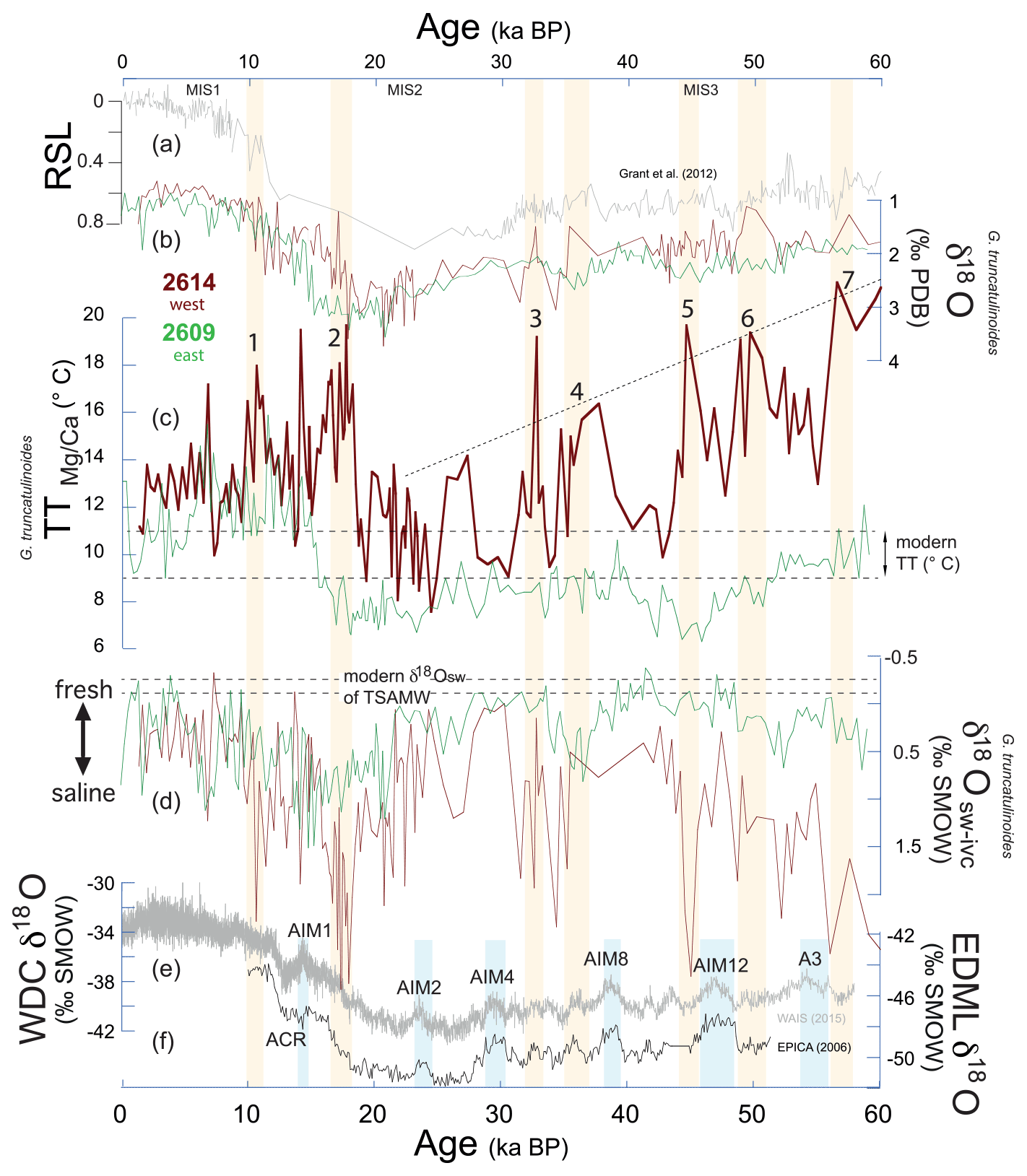
Figure 5Hydrographic development at thermocline depth over the last 60 kyr. Colored curves represent this study, while grey and black curves represent reference records. (a) Relative sea level curve of Grant et al. (2012) (in ‰). (b) Thermocline δ18OG. truncatulinoides records at the western (brown; core 2614) and the eastern (green; core 2609) core locations. (c) TT records derived from G. truncatulinoides (brown: core 2614; green: core 2609). (d) Thermocline salinity approximations (δ18Osw-ivc) at the western (brown) and eastern (green) core locations. (e) West Antarctic Ice Sheet Divide Core (grey; WAIS Divide Project Members, 2015) and (f) EDML (black; EPICA Community Members, 2006) δ18O records as reference for the Southern Hemisphere climate signal. Blue shading shows the Antarctic Isotope Maxima (AIM). Red shading shows the prominent thermocline warming pulses and changes to high salinities at thermocline depth (black numbers). Dashed lines are the modern annual TT range at 50–100 m water depth (Locarnini et al., 2019) and modern δ18Osw range of TSAMW (Richardson et al., 2019). MIS stands for Marine Isotope Stages 1–3 (Martinson et al., 1987). ACR stands for Antarctic Cold Reversal.
We hence hypothesize that the O. universa SST signal is seasonally biased towards the austral summer season. We note also that the entire core 2609 SST record matches the SSTLDI record from nearby core MD03-2607 reasonably well, with similar absolute temperature estimates (∼11–24 ∘C) and particularly similar deglacial amplitudes of up to 7 ∘C (Fig. 4c). Both the SSTLDI and SST estimates are warmer by ∼4 ∘C than the alkenone-based SST estimate from cores MD03-2607 (Lopes dos Santos et al., 2012) and MD03-2611 (Calvo et al., 2007; S, E; Fig. 1), likely due to the fact that SST reflects the cooler early spring conditions.
4.2 Thermocline temperature and salinity development over the last 60 kyr
All raw analytical data of cores 2614 and 2609 versus core depth are presented in the Supplement (Figs. S6 and S7). Over the last 60 kyr, the development at thermocline depth in the western study area south of Cape Pasley (core 2614) differs substantially from the eastern area, with prominent and rapid high-amplitude changes in TT and the according δ18Osw-ivc in the western area. The proxy records from the eastern core 2609 instead appear rather muted, cooler, and fresher (Fig. 5c and d).
During MIS 3, the TT in western core 2614 ranges between 10 and 21 ∘C, revealing a long-term cooling trend from ∼20 ∘C at 60 ka BP on average to ∼11 ∘C at ∼23 ka BP (Fig. 5c). This cooling trend is accompanied by high-amplitude TT variations even exceeding 5 ∘C. The TT and thermocline depth δ18Osw-ivc minima correspond to the modern TT (9–11 ∘C; cf. Fig. 2) and δ18Osw ranges at core location 2614 (Richardson et al., 2019), while distinct warming pulses at thermocline depth and saline conditions exceed modern conditions by up to ∼10 ∘C and ∼2 ‰, respectively (Fig. 5c and d). Although some of these TT warming pulses are only represented by single data points (due to rare foraminiferal sample material), we assess them as robust as the peaks are mostly supported by several δ18OG. truncatulinoides and δ13CG. truncatulinoides excursions to light values (Fig. 5b).
In the eastern core 2609, the MIS3 TT ranges between ∼7 and 11 ∘C, which is cooler by a maximum of 2 ∘C than the modern TT range of 9–11 ∘C (cf. Fig. 2). The thermocline depth δ18Osw-ivc values (−0.5 ‰ to ∼0.5 ‰) are mostly equal to or more positive than the modern value (Richardson et al., 2019; cf. Fig. 5d) but remain clearly fresher by up to 2 ‰ and less variable than at the western core (0 ‰–2 ‰). During MIS 2 and during the LGM in particular, the conditions at thermocline depth at core 2609 are cooler than modern temperatures by ∼2 ∘C, while remaining fresher and lower in amplitude compared to the clearly more variable and warmer thermocline conditions at core 2614 (Fig. 5c and d). The western location rather exhibits short-term TT variations between ∼8 and ∼13 ∘C, which is close to the modern TT in the region. Relative salinity varied correspondingly (0.5 ‰–1.5 ‰).
In the western study area, the deglaciation is characterized by rapid and prominent changes in thermocline conditions (Fig. 5c). Increases in TT by up to 10 to a maximum of 20 ∘C and in δ18Osw-ivc by up to 2.5 ‰ in amplitude occur during the early Heinrich Stadial 1, the early Bølling/Allerød, and the Preboreal. In contrast, the deglacial change in the eastern study area lags behind the western development and is less prominent, with TT rising from 7 to 12 ∘C in line with the Southern Hemisphere deglacial climate change as reflected in the EDML δ18O record (EPICA Community Members, 2006; Fig. 5f).
The Holocene is characterized in both regions by subtle variations in TT and corresponding δ18Osw-ivc. The western core shows higher TT (∼12–14 ∘C and warmer-than-modern conditions) than the eastern core (∼10–12 ∘C, rather similar to modern conditions at thermocline depth), while the salinity (0 ‰ to 0.5 ‰) in both areas appears rather similar and close to the modern values (which is 34.8–35.1 in the western core and 34.7–34.9 in the eastern core; Fig. 5c and d).
4.3 Sea surface–thermocline interrelationships reflecting Leeuwin Current dynamics
We interpret the SST and surface δ18Osw-ivc data derived from O. universa in terms of changes in the surface mixed layer, which is dominated by STSW (contributions of Leeuwin Current-transported TSW and South Indian Ocean Current-transported SICW) at the western core location and by the South Australian Current (SAC) in the eastern study area (Fig. 1). The thermocline-dwelling G. truncatulinoides proxy data instead reveal changes in the underlying Central Water, which comprises SABCW and Tasman Subantarctic Mode Water (TSAMW). The boundary between STSW and Central Water defines the interface between the eastward-directed Leeuwin Current System and the westward flow of the Flinders Current System (see Fig. 2b; see Sect. 2.2).
To assess the dynamics of the Leeuwin Current-transported STSW and its interaction with both the surface SAC and the underlying SABCW/TSAMW south of Australia through time, we calculated the vertical temperature gradients at both core locations (see Sect. 3.3). The vertical temperature gradient (ΔTSST-TT) provides insight into the thermocline depth, with small (large) ΔTSST-TT pointing to a shallow (steep) thermal gradient and a deep (shallow) thermocline with accompanying strong (weak) vertical mixing. In conjunction with the lateral gradients at both sea surface (ΔSSTwest-east) and thermocline depths (ΔTTwest-east; Fig. 6a and b), which define the regional differences at the two depth levels, we derive insight into how the Leeuwin Current System developed spatially in relation to the Flinders Current System during different climate regimes. The similarity (R=0.87) between the ΔTTwest-east record (Fig. 6b) and the TT record of the western core 2614 (Fig. 5c) pinpoints that it is the thermocline changes in the western area that are crucial to the oceanographic setting south of Australia and best reflect the relative presence of the different water masses.

Figure 6Variability of lateral and vertical temperature gradients south of Australia in comparison to other proxy records over the last 60 kyr. (a) Vertical temperature gradients (ΔTSST-TT) between sea surface and thermocline reflecting thermocline changes in the western (red) and eastern (green) study areas in line with migrations of the STF. The small double arrow along the y axis marks the modern vertical gradient (30–350 m) in the west (Locarnini et al., 2019). (b) Lateral (west–east) 13-point smoothed temperature gradients at the sea surface (grey) and at thermocline depth (black) reflecting Leeuwin Current strength, underlain by the raw data (equally sampled at 0.2 kyr spacings using AnalySeries 2.0; Paillard et al., 1996). Stippled lines in (a) and (b) indicate long-term trends. (c) N. pachyderma dextral and (d) G. ruber percentages of core MD03-2611 from De Deckker et al. (2012) reflecting lateral migrations of the STF and changes in Leeuwin Current strength, respectively. (e) West Antarctic Ice Sheet Divide Core δ18O record (WAIS Divide Project Members, 2015) as a reference for the Southern Hemisphere climate signal. Orange shading shows short time periods of a strong Leeuwin Current. A3 is the Antarctic warming event. AIM stands for Antarctic Isotope Maxima. MIS stands for Marine Isotope Stages 1–3 (Martinson et al., 1987). ACR stands for Antarctic Cold Reversal.
4.3.1 MIS3
The oceanographic setting as it exists today was considerably different during the early MIS3 (∼60–45 ka BP), with tangible differences between both regions. The thermocline was generally deeper (Fig. 6a), and the thermocline waters were considerably warmer and more saline in the western region than in the eastern region (Fig. 5c and d), pointing to an overall thick STSW in line with a strong Leeuwin Current. The SST conditions were rather similar in both areas during these times (Figs. 4c and 6a). In the western core 2614, we observe five time periods of thermocline warming and deepening during the extreme cool climate conditions in Antarctica (see EPICA Community Members, 2006; WAIS Divide Project Members, 2013) at ∼58.8–55.8, ∼50.8–48.4, ∼46.6–44.2, ∼37.4–34.2, and ∼33.0–31.4 ka BP (termed 7 to 3 in Figs. 5c and 6b). These warm events at thermocline depth were likely related to the strong southward transfer of tropical heat via the Leeuwin Current and the poleward shift of the STF. On average, they become cooler towards the younger part of the core, supporting the notion of (i) a gradually shoaling thermocline depth (ΔTSST-TT) at the western core 2614 and (ii) the narrowing of the lateral temperature gradient at thermocline depth (Δ TTwest-east) from 13 to 3 ∘C on average during the course of MIS3 (Fig. 6b). Figure 7a illustrates the straight relationship between core 2614 ΔTSST-TT and ΔTTwest-east.
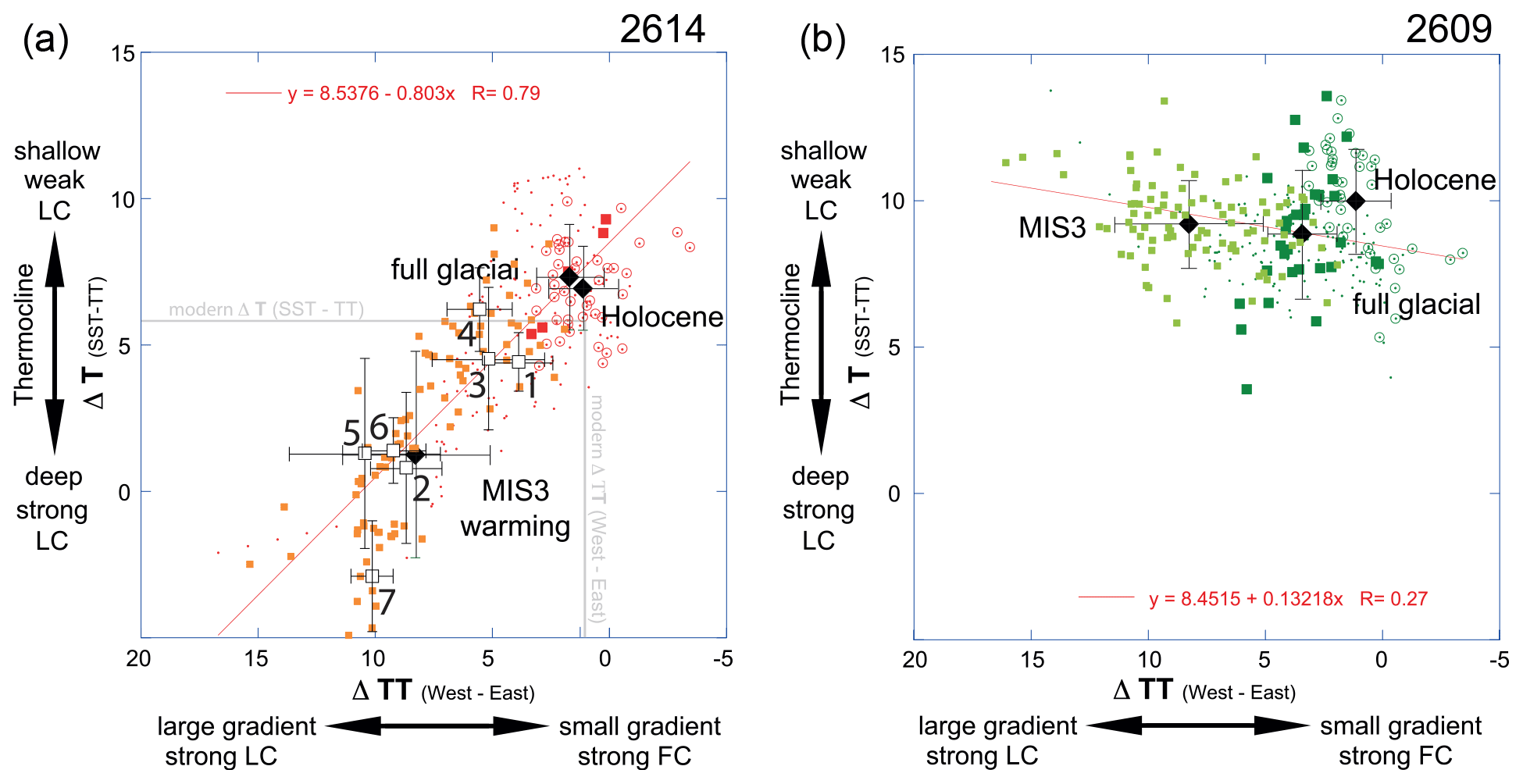
Figure 7Vertical temperature versus lateral thermocline temperature gradient as expression of Leeuwin Current System variability. The vertical temperature gradient (ΔTSST-TT; in ∘C) provides insight into the thermocline depth, with low (high) ΔTSST-TT pointing to a deep (shallow) thermocline. The lateral gradient at thermocline depth (ΔTTwest-east; in ∘C) defines how the Leeuwin Current developed in relation to the Flinders Current. (a) Western core 2614 showing a well-defined relationship between ΔTSST-TT and ΔTTwest-east (R=0.8). Prominent MIS3 thermocline warming periods (orange symbols; white squares are averages, numbered from 7 to 1) point to a strong Leeuwin Current, which weakened across MIS3 (black diamonds show averages) approaching LGM (red squares) and Holocene conditions (red circles; black diamonds show averages). (b) Eastern core 2609 lacks a relationship between ΔTSST-TT and ΔTTwest-east, implying that the Leeuwin Current is not affecting this study site over time.
Overall, the rapidly developing (within centuries) thermocline warming events are intercalated by times of cool, fresh, and shallow thermocline conditions. These conditions predominated during Antarctic Isotope Maxima (A3, AIM12, AIM11, and AIM4), when the sea surface in particular experienced warming by a couple of degrees, pointing to the presence of a shallow and weak Leeuwin Current in the west rather analogous to a modern austral summer scenario (Figs. 4c and 6b).
We argue that the highly variable sea surface and thermocline conditions during MIS3 were likely related to rapid shifts of the oceanic and atmospheric frontal systems: (i) the poleward movement of the Subtropical Ridge and the STF, promoting an enhanced STSW contribution in relation to a stronger Leeuwin Current, and (ii) the successive equatorward frontal migration, leading into the full glacial conditions with an overall weak Leeuwin Current (see discussion below). This is in line with Moros et al. (2009) and De Deckker et al. (2012), who related reduced (increased) Leeuwin Current strength to the northward (southward) displacement of the STF prompted by the strengthening (weakening) of the westerlies in response to changing low- to high-latitude pressure and thermal gradients (Fig. 6c and d). The comparison to the Wu et al. (2021) proxy record of bottom current strength in the Drake Passage (Fig. 8c) further illustrates that times of a strong Leeuwin Current (thermocline warming events 7 to 3; orange shading in Fig. 8) were mostly accompanied by a weakly developed ACC. A weak Leeuwin Current instead predominated during times of ACC acceleration to higher flow speeds during warm intervals in the Southern Hemisphere (A3, AIM12, AIM11, and AIM 4).
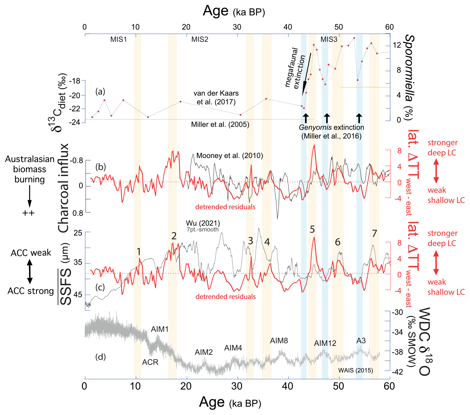
Figure 8Variability of Leeuwin Current strength in comparison to Australian megafaunal extinction, biomass burning, and Antarctic Circumpolar Current (ACC) strength over the last 60 kyr. (a) Record of dung fungus Sporormiella percentages in western core 2614, pointing to the Australian megafaunal population collapse at ∼45 to 43.1 ka BP (van der Kaars et al., 2017). The yellow lines depict the Australian emu Dromaius dietary δ13C change documenting a permanent change in food sources (Miller et al., 2005). The three black arrows indicate most probable extinction dates of the Australian megafaunal bird Genyornis newtoni at ∼54, ∼47, and ∼43 ka BP (Miller et al., 2016). (b) Residuals of detrended lateral (west–east) temperature gradients at thermocline depth reflecting Leeuwin Current strength (red; detrended with Past4 software; https://www.nhm.uio.no/english/research/resources/past/, last access: 10 November 2022), underlain by the Mooney et al. (2010) record of Australian biomass burning. (c) Residuals of detrended lateral (west–east) temperature gradients at thermocline depth reflecting Leeuwin Current strength (red), underlain by the sortable silt record (SSFS; 7 pt-smooth) of Drake Passage sediment core PS97-85 reflecting the strength variability of the ACC (Wu et al., 2021). (d) West Antarctic Ice Sheet Divide Core δ18O record (WAIS Divide Project Members, 2015) as a reference for the Southern Hemisphere climate signal. Orange shading shows short time periods of a strong Leeuwin Current, mostly accompanied by less Australian biomass burning and ACC weakening. Blue shading shows an Antarctic warming event (A3) and Antarctic Isotope Maxima (AIM 12, 10). MIS stands for Marine Isotope Stages 1–3. ACR stands for Antarctic Cold Reversal.
Strength variations in the ACC are commonly attributed to changes in the Southern Westerly Wind Belt (SWW; Lamy et al., 2015) associated with northward shifts of the Subantarctic Front (Roberts et al., 2017). However, model simulations imply that changes in the westerlies alone were likely insufficient to influence high-amplitude changes in ACC speeds (Gottschalk et al., 2015). Wu et al. (2021) suggested that the millennial-scale ACC flow speed variations were closely linked to variations of Antarctic sea ice extent (maxima in ACC strength at major winter sea ice retreat; weaker ACC at a more extensive sea ice cover), closely related to the strength and latitudinal position of the SWW (Toggweiler et al., 2006), oceanic frontal shifts (Gersonde et al., 2005), and buoyancy forcing (Shi et al., 2020).
At the eastern core location 2609, the thermocline and halocline changes vary only marginally (TT amplitude of ∼3 ∘C compared to >10 ∘C at the western site; δ18Osw-ivc amplitude of ∼1 ‰ compared to >3 ‰ at the western site) with no apparent relationship to the short-term MIS3 climate variability (which is likely due to our low sampling coverage; Fig. 5c and d). The relationship between ΔTSST-TT and ΔTTwest-east is not well expressed and clearly different from core 2614 (Figs. 6a and b and 7). We note that even during most intensive STSW transport via the Leeuwin Current during the MIS 3 thermocline warming periods 7, 6, 5, 4, and 3, the eastern core location was hardly affected. We speculate that the Leeuwin Current (defined as “southward shelf edge flow off Western Australia that turns around Cape Leeuwin and penetrates eastward as far as the central Great Australian Bight”; Ridgway and Condie, 2004) was not present at the core 2609 location at all. Instead, it is likely the South Australian Current (defined as “winter shelf edge flow largely driven by reversing wind … that originates from a gravity outflow from the eastern Great Australian Bight and spreads eastward as far as the eastern edge of Bass Strait”; Ridgway and Condie, 2004) that determines when the core 2609 SST approaches that of core 2614. Approaching SST conditions at both study sites with according ΔSST minima occurred consistently during the MIS 3 warming periods 7, 6, 5, and 3, implying that the formation of the South Australian Current intensified at times of a strong Leeuwin Current (Fig. 6b).
The differences in thermocline development at both core locations might have been fostered by the functioning of the Subtropical Ridge (∼30 and S; see, e.g., Drosdowsky, 2005). We argue that the eastern core 2609 at ∼39∘ S is more effectively influenced by temporal and spatial changes in the Subtropical Ridge as it is closer to the rainy westerlies than the western core 2614 at S. Congruently, the core 2609 surface and thermocline δ18Osw-ivc records point to overall fresher sea surface conditions during MIS3 cool periods than core 2614. A new pollen record from between our core locations (De Deckker et al., 2021; core MD03-2607; Fig. 1) unfortunately does not capture the rapid MIS 3 variability we see in our oceanographic reconstructions, although it does reveal subtle changes in regional vegetation and fluvial discharge patterns in the Murray–Darling Basin.
4.3.2 MIS2 and LGM
At the western core location 2614, the few but relatively heavy δ18OO. universa data point to rather cool sea surface conditions during the LGM (Fig. 4b). The thermocline conditions (∼8–13 ∘C) appear cool but variable (Fig. 5c). At the eastern core location 2609, the thermocline was instead even cooler than modern conditions by ∼2 ∘C, fresher, and low in amplitude. Overall, we note a shallow thermocline at core location 2609 (Fig. 6a) and a low west–east gradient at thermocline depth (Fig. 6b), pointing to a narrower, shallower, and weaker Leeuwin Current influencing the western study area. This is in accordance with Martinez et al. (1999), who described the northward dislocation and shrinking of the Indo-Pacific Warm Pool during the LGM, which should have significantly reduced the export of tropical low saline and warm ITW water via the Leeuwin Current and consequently should have reduced the geostrophic gradient similar to El Niño conditions (Meyers et al., 1995; Feng et al., 2003).
The northward movement of the STF (Howard and Prell, 1992; Martinez et al., 1999; Passlow et al., 1997; Findlay and Flores, 2000; Nürnberg and Groeneveld; 2006) and the northward shift of the Subtropical Ridge by 2–3∘ in latitude (Kawahata, 2002) during full glacial climate conditions likely strengthened the West Australian Current as an eastern boundary current, introducing higher portions of cool SICW into the Leeuwin Current (Wandres, 2018; Barrows and Juggins, 2005). The enhanced glacial dominance of the West Australian Current implies that wind conditions became favorable for its flow and/or the alongshore geopotential pressure gradient, which drives the Leeuwin Current, was excelled by the wind stress from the coastal southwesterly winds (Wandres, 2018; Spooner et al., 2011). The resulting glacial reduction of southward heat transfer should have resulted in the significant reduction of cloud cover and hence precipitation. Courtillat et al. (2020) noted that today's rainfall is more important in the cool winter months, when the subtropical highs (or subtropical ridges) move to the north and the cold fronts embedded in the westerly circulation bring moisture over the continent (Suppiah, 1992).
At the eastern core location 2609, the relatively fresh and cool conditions at both surface and thermocline depth, the shallow thermocline, and the small ΔTTwest-east gradient at times of a narrower and shallower Leeuwin Current (Fig. 6a and b) imply that during the LGM (i) the formation of the South Australian Current was rather inactive and (ii) SABCW increasingly formed along the northerly displaced STF by convective overturning and subduction (Richardson et al., 2018) during times of intensified westerlies (e.g., Kaiser and Lamy, 2010) and was carried northward by a glacially strengthened Flinders Current.
Our marine proxy records allow us to draw new conclusions on the oceanic and climatic evolution south of Australia during MIS3 and 2, which confirms (but also adds to) the climatic information available from low-resolution Australian terrestrial records. Petherick et al. (2013) concluded from a large compilation of vegetational data that the glacial climate of the Australian temperate region was relatively cool with the expansion of grasslands and increased fluvial activity in the Murray–Darling Basin, likely in response to a northerly shift of the Southern Ocean oceanic frontal system. Expanded sea ice around Antarctica, and a concomitant influx of subantarctic waters along the southeast and southwest Australian coasts occurred at the same time. Notably, the cooling and aridification in Australia during the LGM (cf. De Deckker et al., 2021) led to pronounced geographic contractions of human populations and the abandonment of large parts of the continent (Williams et al., 2013), followed by a deglacial re-expansion of populations (Tobler et al., 2017).
4.3.3 Deglaciation
The deglacial warming in Antarctica was accompanied by sea ice retreat, sea level rise, and rapidly increasing SSTs in the Southern Ocean between ∼18 and 15 ka BP (Barrows et al., 2007; Pedro et al., 2011). In both our cores, the beginning of the deglaciation is defined by the common decline in planktonic δ18O-values (G. ruber, O. universa, G. truncatulinoides) starting at ∼18 ka BP (Fig. 3a–c). It is further characterized by sea surface warming closely related to the Southern Hemisphere climate signal (WAIS Divide Project Members, 2013; EPICA Community Members, 2006) with SST being overall warmer in the western core region and rather congruent to other deglacial SST proxy records from the region (Fig. 4c; Lopes dos Santos et al., 2013; Calvo et al., 2007).
The deglacial thermocline development, however, differs between core locations, with a rapid (within a few centuries) and variable change to high TT and high salinities from ∼18.3–15.8 ka BP in the western area, similar to the thermocline deepening and warming episodes described earlier for MIS3 (Fig. 5c). The enhanced lateral temperature gradient at thermocline depth (ΔTwest-east) and the lowered vertical (ΔTSST-TT) temperature gradient at the western core 2614 (Fig. 6a and b) point to the rapid formation of a deep thermocline in response to a strengthened Leeuwin Current, and the greater influx of ITW waters at the expense of SICW contributions during the times of poleward migration of the STF. A second major, albeit less prominent, advance of the Leeuwin Current took place at ∼11.1–9.9 ka BP before relatively weak Holocene conditions were achieved. These deglacial intensifications of the Leeuwin Current were synchronous to foraminiferal assemblage changes detected by De Deckker et al. (2012) on Great Australian Bight core MD03-2611 (cf. Fig. 1), which were interpreted in terms of southward migrations of the STF (Fig. 6c and d).
At the eastern core 2609, the prominent deglacial changes in the thermocline are missing, suggesting that the Leeuwin Current did not reach the eastern study area (Figs. 4 and 5). Slight increases in SST during these short time periods of a strong Leeuwin Current imply that the formation of the South Australian Current might have been active though. The vegetational record from the Australian temperate region showing the expansion of arboreal taxa at the expense of herbs and grasses points to a gradual deglacial (∼18–12 ka BP) rise in air temperature and precipitation in the Murray–Darling Basin and the strengthened influence of the westerlies across the southern Australian temperate zone (Fletcher and Moreno, 2011).
4.3.4 Holocene
The oceanographic development during the Holocene closely corresponds to the vegetational and climatic development of Australia. Most importantly, the thermocline off southern Australia was considerably shallower during the Holocene compared to the prominent MIS3 and deglacial periods of Leeuwin Current intensification, pointing to a comparably weak Leeuwin Current (Fig. 6a and b). At the sea surface, the eastern study area was apparently warmer and more saline than the western area (Fig. 4c). On land, Petherick et al. (2013) described an early Holocene expansion of sclerophyll woodland and rainforest taxa across the Australian temperate region after ∼12 ka BP, which they related to increasing air temperature and a spatially heterogeneous hydroclimate with increased effective precipitation (cf. Williams et al., 2013; Kiernan et al., 2010; Moss et al., 2013), a widespread re-vegetation of the highlands, and a return to full interglacial conditions. At the same time, the East Australian Current reinvigorated, flowing south down the eastern coast of Australia and seasonally affecting the southern coast (Bostock et al., 2006).
The differential behavior at surface and thermocline depths became most pronounced after ∼6 ka BP, when the thermocline at the eastern core location 2609 became distinctly shallower than in the western study area, while SST continued to increase. We relate the warmer and more saline late Holocene conditions at the sea surface in the east (Fig. 4c and d) to intensified surface heating near the eastern edge of the Great Australian Bight during austral summer (cf. Herzfeld and Tomzcak, 1997). These shallow waters then spread eastward over the shelf and continued to flow as the South Australian Current towards Bass Strait (Middleton and Platov, 2003; Ridgeway and Condie, 2004; cf. Fig. 1). After ∼6 ka, Petherick et al. (2013) also describe a higher-frequency climatic variability in the Australian temperate region and a spatial patterning of moisture balance changes that possibly reflect the increasing influence of ENSO climate variability originating in the equatorial Pacific (Moy et al., 2002)
At thermocline depth, the development of gradually declining TT and salinities appear rather similar in the eastern and western study areas over the Holocene, although the western area remained warmer by ∼2 ∘C and the thermocline was deeper due to an active but relatively weak Leeuwin Current (Fig. 5c and d). These conditions gradually approached the modern situation and imply a strengthened influence of the SABCW and SAMW in the course of the Holocene, transported by an intensified Flinders Current–Leeuwin Undercurrent system. The eastern study area was more affected, likely because the Subtropical Ridge gradually shifted northward across the core 2609 location in response to the increasing influence of ENSO climate variability. From geochemical proxy data of annually banded massive Porites corals from Papua New Guinea, Tudhope et al. (2001) concluded that ENSO developed from weak conditions in the early to mid-Holocene to conditions that are variable but stronger than during the past 150 000 years today, mainly driven by effects of orbital precession.
4.4 Australian megafaunal extinction in relation to ocean/climate dynamics
Palynological studies on our western core 2614 record a substantial decline of the dung fungus Sporormiella, a proxy for herbivore biomass, which was taken as evidence for the prominent Australian megafaunal population collapse from ∼45 to 43.1 ka BP (van der Kaars et al., 2017; Fig. 8a). Climate change likely played a significant role in most of the disappearance events of the continent's megafauna during the Pleistocene, while human involvement appears likely for the last megafaunal population collapse after ∼45 ka BP in particular, but this is still debated (Wroe et al., 2013).
A new chronology constrains the early dispersal of modern humans out of Africa across southern Asia into “Sahul” (northern Australia and New Guinea connected by a land bridge at times of glacially lowered sea level; see Saltré et al., 2016) to ∼65–50 ka BP (Clarkson et al., 2017; Tobler et al., 2017). The further settlement comprised a single, rapid (within a few thousand years; Tobler et al., 2017) migration along the eastern and western coasts, with Aboriginal Australians reaching the south of Australia by ∼49–45 ka BP. It is also clear that humans were present in Tasmania by ∼39 ka BP (Allen and O'Connell, 2014) and in the arid center of Australia by ∼35 ka BP (Smith, 2013). This places the initial human colonization of Australia clearly before the continent-wide extinction of the megafauna (cf. Saltré et al., 2016). Rule et al. (2012) and van der Kaars et al. (2017) claimed that human arrival causing overhunting, vegetation change due to landscape burning, or a combination thereof was the primary extinction cause rather than climate change. Brook and Johnson (2006) showed with model simulations that species with low population growth rates, such as large-bodied mammals in Australia, might have been easily exterminated by even small groups of hunter-gatherers using stone-based tools. Saltré et al. (2016) also hypothesized that climate change was not responsible for late Quaternary (last 120 kyr) megafauna extinctions in Australia, as they appeared to be independent of climate aridity and variability.
Our record of detrended ΔTTwest-east, which approximates the strength of the Leeuwin Current, provides additional views on these issues. It shows a robust covariance on millennial to centennial timescales from ∼60 to 20 ka BP to a charcoal composite record reflecting biomass burning in the Australasian region (Mooney et al., 2010; Fig. 8b). Commonly, fewer fires appeared during periods associated with an intensified Leeuwin Current, a southward-located STF and Subtropical Ridge, and wetter conditions in the Australasian region at times of a weakened ACC (cf. Fig. 8b and c). The consistent timing of changes in both ocean dynamics and biomass burning over such a long period even prior to the arrival of humans in Australia (see Singh et al., 1981) suggests a strong coupling between climate-modulated changes related to the Leeuwin Current and changes in terrestrial vegetation productivity and distribution. This might have been an important factor for controlling Australasian fire regimes (Mooney et al., 2010). We hence argue that it is the joint interplay between natural ocean and climate variability, vegetational response, and human interference that caused the Australian megafaunal extinction.
Figure 8a shows the Sporormiella record of western core 2614 (van der Kaars et al., 2017) in comparison to our detrended record of Leeuwin Current variability. It is evident that before ∼45–43.1 ka BP the Sporormiella abundances were highly variable, placing Sporormiella abundance maxima (>10 %–13 %) into times of extensive thermocline expansion and the strong southward transfer of tropical heat via the Leeuwin Current (warming phases 7, 6, and 5; Fig. 8a and b). This is when Antarctica cooled (WAIS Divide Project Members, 2013) and the ACC weakened, likely in response to sea ice expansion (Wu et al., 2021; Fig. 8c and d). Sporormiella minima ( %) instead consistently occurred during times of a shallow thermocline and a weakened Leeuwin Current, with percentages becoming lower stepwise during Antarctic warm periods A3 (∼7 %) and AIM12 (∼6 %) until they reach their lowest values (∼2 %) during AIM11 at ∼45–43.1 ka BP (Fig. 8a).
The successive decline of Sporormiella during Antarctic warm periods and its rapid recuperation in between during times of Antarctic cooling, sea ice expansion, and ACC slowdown is mirrored in the decline of the Australian megafaunal bird Genyornis newtoni. From widespread eggshell fragments of Genyornis exhibiting diagnostic burn patterns, Miller et al. (2016) concluded that humans depredating and cooking eggs significantly reduced the reproductive success of Genyornis. They dated the egg predation and the related extinction of Genyornis to ∼47 ka BP, although they admitted that an age range from ∼54 to 43 ka BP could not confidently be excluded (Fig. 8a). This places the given extinction dates of Genyornis into the periods of prominent declines in Sporormiella abundances (A3, AIM12, AIM11) and hence into periods of a weak Leeuwin Current system, while in the warming Southern Ocean (WAIS Divide Project Members, 2013) sea ice extension shrank and the ACC strengthened (Wu et al., 2021; Fig. 8c).
The tight coupling between oceanographic changes and changes in the Australian megafauna brings ocean dynamics as an important player into the game. We hypothesize that the apparent rapid variations in the ocean–climate system from ∼60 to ∼43 ka BP with an overall tendency towards a weakening of the Leeuwin Current and the equatorward migration of the Southern Hemisphere frontal system (Fig. 8) must have caused considerable climatic and ecosystem response in Australia, with negative aftereffects on the continent's megafauna. A recuperation of the megafauna, however, is documented (and expected) by the increasing Sporormiella abundances during each of the short time periods 7, 6, and 5 of an intensified southward transfer of tropical heat via the Leeuwin Current and poleward shift of the Subtropical Ridge (Fig. 8b), even though human impact should have persisted or even raised during this period.
The final extinction phase defined to ∼45–43.1 ka BP on the basis of the core 2614 Sporormiella record (van der Kaars et al., 2017) and supported by other studies (e.g., Miller et al., 2005, 2016; Rule et al., 2012) appeared synchronous to the significant decline in the core 2614 thermocline temperature, salinity, and depth; the reduction of ΔTTwest-east by more than 10 ∘C; and the clearly warmer and more saline sea surface conditions in the western study area, while the eastern sea surface remained cool and fresh (Figs. 5 and 6). This all points to the drastic weakening and shoaling of the Leeuwin Current (analogous to the modern austral summer conditions) with the STF being pushed to the north and a larger impact of the glacial Southern Ocean via an enhanced Flinders Current. The significant reorganization of the ocean circulation south of Australia at ∼45–43.1 ka BP is accompanied by a transient change in climate and vegetation in Australia. Bowler et al. (2012) described a drying trend in SE Australia (Willandra Lakes) since ∼45 ka, synchronous with the weakening of the Australian monsoon (Johnson et al., 1999) and also visible in the Mooney et al. (2010) charcoal record (Fig. 8b). The dietary δ13C change in the Australian emu Dromaius novaehollandiae population at that time (Fig. 8a) also points to the reorganization of vegetation communities across the Australian semiarid zone (Miller et al., 2005). The abrupt decline in C4 plants between ∼44 and 42 ka BP observed in core MD03-2607, however, was interpreted by Lopes dos Santos et al. (2013) not in terms of climate change but in terms of a large ecological change, primarily caused by the absence of the megafaunal browsers due to extinction. The extinction left increased C3 vegetation biomass in the landscape, which would have fostered fires, eventually aided by human activities (Lopes dos Santos et al., 2013).
We hypothesize, alternatively, that the centennial-scale severe change in the ocean–climate system beginning at ∼45 ka BP must have had aftereffects on the continental environment. We argue that the megafauna, which might have been significantly decimated by human activity at that point, likely did not keep track with the rapidly increasing ecological stress and was no longer able to adapt to the changing conditions related to the weakening of the Leeuwin Current. Humans might indeed have effectively contributed to the extinction of the Australian megafauna as previously suggested (e.g., Rule et al., 2012; Miller et al., 2016; van der Kaars et al., 2017), but the ocean–climate dynamics provide an important prerequisite and amplifying factor until a tipping point was reached, after which faunal recuperation no longer happened.
The Leeuwin Current as important conduit for the poleward heat transport and inter-ocean water exchange between the tropical and the subantarctic ocean areas is highly crucial for the climatic and vegetational evolution of Australia. The thermocline south of Australia reflects changes between the eastward-directed Leeuwin Current System transporting subtropical waters and the westward flow of the Flinders Current System, which brings subantarctic waters into the region.
During MIS3, the centennial-scale variations in the Leeuwin Current and the related migrations of the Southern Hemisphere frontal system reveal a tendency towards weakening of the Leeuwin Current. It was, instead, strongly developed during Antarctic cool periods at times when the ACC weakened in response to the expanded sea ice cover around Antarctica.
During the LGM we note an even narrower, shallower, and weaker Leeuwin Current, likely in response to the northward dislocation and shrinking of the Indo-Pacific Warm Pool, which significantly reduced the export of tropical low saline and warm ITW water. The northward shift of the Subtropical Ridge during the LGM likely strengthened the West Australian Current, introducing higher portions of cool SICW into the Leeuwin Current.
During deglacial times, the enhanced vertical and lateral temperature gradients point to the rapid formation of a deep thermocline in response to a strengthened Leeuwin Current, and the greater influx of ITW waters at the expense of SICW contributions at times of poleward migration of the STF.
During the Holocene, the thermocline off southern Australia was considerably shallower compared to the prominent MIS3 and deglacial periods of Leeuwin Current intensification, pointing to a comparably weak Leeuwin Current. After ∼6 ka BP, the intensified surface heating near the eastern edge of the Great Australian Bight suggests an intensified South Australian Current. At thermocline depth, the strengthened influence of the SABCW and SAMW is visible, transported by an intensified Flinders Current–Leeuwin Undercurrent system.
Overall, the Leeuwin Current variability from ∼60–20 ka BP captures the biomass burning development in Australasia with less fire when the Leeuwin Current intensified, the STF and the Subtropical Ridge moved southward creating wetter conditions across Australia, and the ACC weakened. The consistent timing of changes suggests that climate-modulated changes related to the Leeuwin Current were likely crucial for driving Australasian fire regimes. As a consequence, we concluded that the concerted action of natural ocean and climate variability, vegetational response, and human interference enhanced the ecological stress on the Australian megafauna until a tipping point was reached at ∼43 ka BP, after which faunal recuperation no longer took place.
Presented data are available online at the Data Publisher for Earth and Environmental Science, PANGAEA (https://doi.org/10.1594/PANGAEA.943197, Nürnberg et al., 2022a; https://doi.org/10.1594/PANGAEA.943199, Nürnberg et al., 2022b).
Cores MD03-2614 and MD03-2609 and remaining sample material are stored in the GEOMAR core and rock repository (https://www.geomar.de/en/centre/central-facilities/tlz/core-rock-repository, last access: 11 November 2022) and can be made available upon request by contacting geosamples@geomar.de.
The supplement related to this article is available online at: https://doi.org/10.5194/cp-18-2483-2022-supplement.
Study conception and design were completed by DN, AK, and KJFM. Data collection was completed by DN, AK, and KJFM. Data analysis and the interpretation of results were completed by DN, AK, KJFM, and CK. Draft manuscript preparation and editing were completed by DN, AK, KJFM and CK. All authors reviewed the results and approved the final version of the paper.
The contact author has declared that none of the authors has any competing interests.
Publisher's note: Copernicus Publications remains neutral with regard to jurisdictional claims in published maps and institutional affiliations.
We thank the captain, crew, and shipboard scientific crew of R/V Marion Dufresne. The studied sediment cores were retrieved during cruise MD131 (AUSCAN campaign) in 2003. We further thank Joachim Schönfeld and lab technicians Nadine Gehre and Sebastian Fessler for their great support. We thank the German Science Foundation (DFG), which provided initial funding for the recovery of the sediment cores. We are thankful to the reviewers, whose comments considerably helped to improve the manuscript.
This research has been supported by the Deutsche Forschungsgemeinschaft (grant no. Nu60/11-1).
The article processing charges for this open-access publication were covered by the GEOMAR Helmholtz Centre for Ocean Research Kiel.
This paper was edited by Luc Beaufort and reviewed by Bradley Opdyke and one anonymous referee.
Allen, J. and O'Connell, J. F.: Both half right: updating the evidence for dating first human arrivals in Sahul, Aust. Archaeol., 79, 86–108, 2014.
Anand, P., Elderfield, H., and Conte, M. H.: Calibration of thermometry in planktonic foraminifera from a sediment trap time series, Paleoceanography, 18, 1050, https://doi.org/10.1029/2002PA000846, 2003.
Bahr, A., Nürnberg, D., Karas, C., and Grützner, J.: Millennial-scale versus long-term dynamics in the surface and subsurface of the western North Atlantic Subtropical Gyre during marine isotope stage 5, Glob. Planet. Change, 111, 77–87, https://doi.org/10.1016/j.gloplacha.2013.08.013, 2013.
Barker, P. M.: The circulation and formation of water masses south of Australia and the inter-annual wind variability along the southern Australian coast, PhD thesis, University of Melbourne, Victoria, Australia, 351 pp., 2004.
Barker, S., Greaves, M., and Elderfield, H.: A study of cleaning procedures used for foraminiferal paleothermometry, Geochem. Geophys. Geosy., 4, 8407, https://doi.org/10.1029/2003GC000559, 2003.
Barrows, T. T. and Juggins, S.: Sea-surface temperatures around the Australian margin and Indian Ocean during the Last Glacial Maximum, Quat. Sci. Rev., 24, 1017–1047, 2005.
Barrows, T. T., Juggins, S., De Deckker, P., Calvo, E., and Pelejero, C.: Long-term sea surface temperature and climate change in the Australian-New Zealand region, Paleoceanography, 22, PA2215, https://doi.org/10.1029/2006PA001328, 2007.
Bé, A. W. H. and Tolderlund, D. S.: Distribution and ecology of living planktonic foraminifera in surface waters of the Atlantic and Indian Oceans, in: The Micropalaeontology of Oceans, edited by: Funnel, B. M. and Riedel, W. R., University Press, Cambridge, 105–149, 1971.
Bemis, B. E., Spero, H. J., Bijma, J., and Lea, D. W.: Reevaluation of the oxygen isotopic composition of planktonic foraminifera: Experimental results and revised paleotemperature equations, Paleoceanography, 13, 150–160, 1998.
Bostock, H. C., Opdyke, B. N., Gagan, M. K., Kiss, A. E., and Fifield, L. K.: Glacial/interglacial changes in the East Australian current, Clim. Dyn., 26, 645–659, https://doi.org/10.1007/s00382-005-0103-7, 2006.
Bowler, J. M., Gillespie, R., Johnston, H., and Boljkovac, K.: Wind v water: Glacial maximum records from the Willandra Lakes, in: Peopled landscapes: archaeological and biogeographic approaches to landscapes, edited by: Haberle, S. and David, B., Terra australis 34, Chapter 13, ANU e-press, https://doi.org/10.22459/TA34.01.2012.13, 2012.
Boyle, E. A. and Keigwin, L. D.: Comparison of Atlantic and Pacific paleochemical records for the last 215 000 years: changes in deep ocean circulation and chemical inventories, Earth Planet. Sci. Lett., 76, 135–150, https://doi.org/10.1016/0012-821X(85)90154-2, 1985.
Boyle, E. A. and Rosenthal, Y.: Chemical hydrography of the South Atlantic during the Last Glacial Maximum: Cd vs. δ13C, in: The South Atlantic: Present and Past Circulation, edited by: Wefer, G., Berger, W. H., Siedler, G., and Webb, D., Springer, Berlin, Heidelberg, 423–443, https://doi.org/10.1007/978-3-642-80353-6_23, 1996.
Brook, B. W. and Johnson, C. N.: Selective hunting of juveniles as a cause of the imperceptible overkill of the Australian Pleistocene megafauna, Alcheringa, 30, 39–48, 2006.
Cai, W., van Rensch, P., and Cowan, T.: Influence of global-scale variability on the Subtropical Ridge over Southeast Australia, J. Clim., 24, 6035–6053, https://doi.org/10.1175/2011JCLI4149.1, 2011.
Caley, T. and Roche, D. M.: Modeling water isotopologues during the last glacial: implications for quantitative paleosalinity reconstruction, Paleoceanography, 30, 739–750, 2015.
Calvo, E., Pelejero, C., De Deckker, P., and Logan, G. A.: Antarctic deglacial pattern in a 30 kyr record of sea surface temperature offshore South Australia, Geophys. Res. Lett., 34, L13707, https://doi.org/10.1029/2007GL029937, 2007.
Church, J. A., Cresswell, G. R., and Godfrey, J. S.: The Leeuwin Current, in: Poleward flows along eastern boundaries, edited by: Neshyba, S. J., Mooers, Ch. N. K., Smith, R. L., and Barber, R. T., Coastal and Estuarine Studies book series, 34, 230–254, https://doi.org/10.1007/978-1-4613-8963-7_16, 1989.
Cirano, M. and Middleton, J. F.: Aspects of the mean wintertime circulation along Australia's southern shelves: numerical studies, J. Phys. Oceanogr., 34, 668–684, 2004.
Clarkson, C., Jacobs, Z., Marwick, B., Fullagar, R., Wallis, L., Smith, M., Roberts, R. G., Hayes, E., Lowe, K., Carah, X., Florin, A. S., McNeil, J., Cox, D., Arnold, L.J., Hua, Q., Huntley, J., Brand, H. E. A., Manne, T., Fairbairn, A., Shulmeister, J., Lyle, L., Salinas, M., Page, M., Connell, K., Park, G., Norman, K., Murphy. T, and Pardoe, C.: Human occupation of northern Australia by 65 000 years ago, Nature, 54, 306, https://doi.org/10.1038/nature22968, 2017.
Cléroux, C., Cortijo, E., and Duplessy, J.-C.: Deep-dwelling foraminifera as thermocline temperature recorders, Geochem. Geophys. Geosy., 8, 4, https://doi.org/10.1029/2006GC001474, 2008.
Courtillat, M., Hallenberger, M., Bassetti, M.-A., Aubert, D., Jeandel, C., Reuning, L., Korpanty, C., Moisette, P., Mounic, S., and Saavedra-Pellitero, M.: New record of dust input and provenance during glacial periods in Western Australia shelf (IODP Expedition 356, Site U1461) from the Middle to Late Pleistocene, Atmosphere, 11, 1251, https://doi.org/10.3390/atmos11111251, 2020.
Cresswell, G. R.: Currents of the continental shelf and upper slope of Tasmania, Pap. Proc. – R. Soc. Tasman., 133, 21–30, 2000.
Cresswell, G. R. and Golding, T. J.: Observations of a southward flowing current in the south-eastern Indian Ocean – Deep Sea Res. Part I, 27, 449–466, 1980.
Cresswell, G. R. and Peterson, J. L.: The Leeuwin Current south of western Australia, Aust. J. Mar. Freshwater Res., 44, 285–303, 1993.
De Deckker, P., Moros, M., Perner, K., and Jansen, E.: Influence of the tropics and southern westerlies on glacial interhemispheric asymmetry, Nat. Geosci., 5, 266–269, 2012.
De Deckker, P., van der Kaars, S., Haberle, S., Hua, Q., and Stuut, J.-B. W.: The pollen record from marine core MD03-2607 from offshore Kangaroo Island spanning the last 125 ka; implications for vegetation changes across the Murray-Darling Basin, Aust. J. Earth Sci., 68, 928–951, https://doi.org/10.1080/08120099.2021.1896578, 2021.
Domingues, C. M., Maltrud, M. E., Wijffels, S. E., Church, J. A., and Tomczak, M.: Simulated Lagrangian pathways between the Leeuwin Current System and the upper ocean circulation of the southeast Indian Ocean, Deep Sea Res. Part II, 54, 797–817, https://doi.org/10.1016/j.dsr2.2006.10.003, 2007.
Drosdowsky, W.: An analysis of Australian seasonal rainfall and teleconnection patterns anomalies: 1950–1987. II: Temporal variability, Int. J. Climatol., 13, 111–149, 2003.
Drosdowsky, W.: The latitude of the subtropical ridge over eastern Australia: The L-index revisited, Int. J. Climatol., 25, 1291–1299, 2005.
Elderfield, H., Vautravers, M., and Cooper, M.: The relationship between shell size and , SrCa, δ18O, and δ13C of species of planktonic foraminifera, Geochem. Geophys. Geosy., 3, 8, https://doi.org/10.1029/2001GC000194, 2002.
EPICA Community Members: One-to-one coupling of glacial climate variability in Greenland and Antarctica, Nature, 444, 195–198, 2006.
Farmer, E. C., Kaplan, A., de Menocal, P. B., and Lynch-Stieglitz, J.: Corroborating ecological depth preferences of planktonic foraminifera in the tropical Atlantic with stable oxygen isotope ratios of core-top specimens, Paleoceanography, 22, PA3205, https://doi.org/10.1029/2006PA001361, 2007.
Feng, M., Meyers, G., Pearce, A., and Wijfells, S.: Annual and interannual variations of the Leeuwin Current at 32∘ S, J. Geophys. Res.-Oceans, 108, 33–55, 2003.
Feng, M., Weller, E., and Hill, K.: The Leeuwin Current, in: A Marine Climate Change Impacts and Adaptation Report Card for Australia 2009, edited by: Poloczanska, E., Hobday, A. J., and Richardson, A., NCCARF Publication 05/09, ISBN: 978-1-921609-03-9, 2009.
Findlay, C. S. and Flores, J. A.: Subtropical Front fluctuations south of Australia ( S, E) for the last 130 ka years based on calcareous nannoplankton, Mar. Micropaleontol., 40, 403–416, 2000.
Fletcher, M.-S. and Moreno, P. I.: Zonally symmetric changes in the strength and position of the Southern Westerlies drove atmospheric CO2 variations over the past 14 k.y., Geology, 39, 419–422, 2011.
Friedrich, O., Schiebel, R., Wilson, P. A., Weldeab, S., Beer, C. J., Cooper, M. J., and Fiebig, J.: Influence of test size, water depth and ecology on , SrCa, δ18O and δ13C in nine modern species of planktic foraminifers, Earth Planet. Sci. Lett., 319–320, 133–145, 2012.
Gersonde, R., Crosta, X., Abelmann, A., and Armand, L.: Sea-surface temperature and sea ice distribution of the Southern Ocean at the EPILOG Last Glacial Maximum – a circum-Antarctic view based on siliceous microfossil records, Quat. Sci. Rev., 24, 869–896, 2005.
Godfrey, J. S. and Ridgway, K. R.: The large-scale environment of the poleward-flowing Leeuwin Current, Western Australia: Longshore steric height patterns, wind stresses and geostrophic flow, J. Phys. Oceanogr., 15, 481–495, 1985.
Gottschalk, J., Skinner, L. C., Misra, S., Waelbroeck, C., Menviel, L., and Timmermann, A.: Abrupt changes in the southern extent of North Atlantic Deep Water during Dansgaard–Oeschger events, Nat. Geosci., 8, 950, https://doi.org/10.1038/NGEO2558, 2015.
Grant, K. M., Rohling, E. J., Bar-Matthews, M., Ayalon, A., Medina-Elizalde, M., Ramsey, C. B., Satow, C., and Roberts, A. P.: Rapid coupling between ice volume and polar temperature over the past 150 000 years, Nature, 491, 744–747, 2012.
Greaves, M., Caillon, N., Rebaubier, H., Bartoli, G., Bohaty, S., Cacho, I., Clarke, L., Cooper, M., Daunt, C., Delaney, M., deMenocal, P., Dutton, A., Eggins, S., Elderfield, H., Garbe-Schönberg, D., Goddard, E., Green, D., Gröneveld, J., Hastings, D., Hathorne, E., Kimoto, K., Klinkhammer, G., Labeyrie, L., Lea, D. W., Marchitto, T., Martínez-Botí, M. A., Mortyn, P. G., Ni, Y., Nürnberg, D., Paradis, G., Pena, L., Quinn, T., Rosenthal, Y., Russell, A., Sagawa, T., Sosdian, S., Stott, L., Tachikawa, K., Tappa, E., Thunell, R., and Wilson, P. A.: Interlaboratory comparison study of calibration standards for foraminiferal thermometry, Geochem. Geophys. Geosy., 9, Q08010, https://doi.org/10.1029/2008GC001974, 2008.
Hathorne, E. C., Alard, O., James, R. H., and Rogers, N. W.: Determination of intratest variability of trace elements in foraminifera by laser ablation inductively coupled plasma-mass spectrometry, Geochem. Geophys. Geosy., 4, 8408, https://doi.org/10.1029/2003GC000539, 2003.
Heaton, T. J., Köhler, P., Butzin, M., Bard, E., Reimer, R. E., Austin, W. E. N., Bronk Ramsey, C., Grootes, P. M., Hughen, K. A., Kromer, B., Reimer, P. J., Adkins, J., Burke, A., Cook, M. S., Olsen, J., and Skinner, L. C.: MARINE20 – The marine radiocarbon age calibration curve (0–55 000 CAL BP), Radiocarbon, 62, 779–820, https://doi.org/10.1017/RDC.2020.68, 2020.
Herzfeld, M. and Tomczak, M.: Numerical modelling of sea surface temperature and circulation in the Great Australian Bight, Progr. Oceanogr., 39, 29–78, 1997.
Holbrook, N. J., Goodwin, I. D., McGregor, S., Molina, E., and Power, S. B.: ENSO to multi-decadal time scale changes in East Australian Current transports and Fort Denison sea level: Oceanic Rossby waves as the connecting mechanism, Deep Sea Res. Part II, 58, 547–558, https://doi.org/10.1016/j.dsr2.2010.06.007, 2011.
Holbrook, N. J., Davidson, J., Feng, M., Hobday, A. J., Lough, J. M., McGregor, S., Power, S., and Risbey, J. S.: El Niño-southern oscillation, in: A Marine Climate Change Impacts and Adaptation Report Card for Australia 2012, edited by: Poloczanska, E., Hobday, A. J., and Richardson, A., NCCARF Publication 05/09, ISBN: 978-1-921609-03-9, 2012.
Holloway, P. E. and Nye, H. C.: Leeuwin Current and wind distributions on the southern part of the Australian North West Shelf between January 1982 and July 1983, Aust. J. Mar. Freshwater Res., 36, 123–137, 1985.
Howard, W. R. and Prell, W. L.: Late Quaternary surface circulation of the southern Indian Ocean and its relationship to orbital variations, Paleoceanography, 7, 79–118, https://doi.org/10.1029/91PA02994, 1992.
Hut, G.: Consultants' group meeting on stable isotope reference samples for geochemical and hydrological investigations, International Atomic Energy Agency (IAEA), 18, 42, https://inis.iaea.org/collection/NCLCollectionStore/_Public/18/075/18075746.pdf?r=1 (last access: 11 November 2022), 1987.
James, N. P. and Bone, Y.: Neritic carbonate sediments in a temperate realm, Southern Australia, Springer, Dordrecht, 254 pp., ISBN: 978-90-481-9288-5, 2011.
James, N. P., Boreen, T. D., Bone, Y., and Feary, D. A.: Holocene carbonate sedimentation on the west Eucla Shelf, Great Australian Bight: a shaved shelf, Sediment. Geol., 90, 161–177, 1994.
Johnson, B. J., Miller, G. H., Fogel, M. L., Magee, J. W., Gagan, M. K., and Chivas, A. R.: 65 000 years of vegetation change in central Australia and the Australian Summer Monsoon, Science, 284, 1150–1152, 1999.
Kaiser, J. and Lamy, F.: Links between Patagonian Ice Sheet fluctuations and Antarctic dust variability during the last glacial period (MIS 4-2), Quat. Sci. Rev., 29, 1464–1471, https://doi.org/10.1016/j.quascirev.2010.03.005, 2010.
Karstensen, J. and Quadfasel, D.: Formation of Southern Hemisphere Thermocline Waters: Water Mass Conversion and Subduction, J. Phys. Oceanogr., 32, 3020–3038, https://doi.org/10.1175/1520-0485(2002)032<3020:FOSHTW>2.0.CO;2, 2002.
Kawahata, H.: Shifts in oceanic and atmospheric boundaries in the Tasman Sea (Southwest Pacific) during the Late Pleistocene: Evidence from organic carbon and lithogenic fluxes, Palaeogeogr. Palaeoclimatol. Palaeoecol., 184, 225–249, https://doi.org/10.1016/S0031-0182(01)00412-6, 2002.
Kiernan, K., Fink, D., Greig, D., and Mifud, C.: Cosmogenic radionuclide chronology of pre-last glacial cycle moraines in the Western Arthur range, Southwest Tasmania, Quat. Sci. Rev., 29, 3286–3297, 2010.
Lamy, F., Arz, H. W., Kilian, R., Lange, C. B., Lembke-Jene, L., Wengler, M., Kaiser, J., Baeza-Urrea, O., Hall, I. R., Harada, N., and Tiedemann, R.: Glacial reduction and millennial-scale variations in Drake Passage through flow, P. Natl. Acad. Sci. USA, 112, 13496–13501, 2015.
Legeckis, R. and Cresswell, G.: Satellite observations of sea-surface temperature fronts off the coast of western and southern Australia, Deep Sea Res., 28A, 297–306, 1981.
Li, Q., James, N.P., Bone, Y., and McGowan, B.: Paleoceanographic significance of recent foraminiferal biofacies on the southern shelf of Western Australia: a preliminary study, Palaeoceanogr. Palaeoclimatol. Palaeoecol., 147, 101–120, 1999.
Lisiecki, E. L. and Raymo, M. E.: A Pliocene-Pleistocene stack of 57 globally distributed benthic δ18O records, Paleoceanography, 20, PA1003, https://doi.org/10.1029/2004PA001071, 2005.
Locarnini, R. A., Mishonov, A. V., Baranova, O. K., Boyer, T. P., Zweng, M. M., Garcia, H. E., Reagan, J. R., Seidov, D., Weathers, K. W., Paver, C. R., and Smolyar, I.V.: World Ocean Atlas 2018, 1, Temperature, edited by: Mishonov, A., NOAA Atlas NESDIS 81, 52 pp., https://www.ncei.noaa.gov/access/world-ocean-atlas-2018/ (last access: 11 November 2022), 2019.
Lohmann, G. P. and Schweitzer, P. N.: Globorotalia truncatulinoides growth and chemistry as probes of the past thermocline: 1. Shell size, Paleoceanography, 5 , 55–75, 1990.
Lopes dos Santos, A. R., Wilkins, D., De Deckker, P., and Schouten, S.: Late Quaternary productivity changes from offshore southern Australia: a biomarker approach, Palaeoceanogr. Palaeoclimatol. Palaeoecol., 363–364, 48–56, 2012.
Lopes dos Santos, A. R., De Deckker, P., Hopmans, E. C., Magee, J. W., Mets, A., Sinninghe Damsté, J. S., and Schouten, S.: Abrupt vegetation change after the Late Quaternary megafaunal extinction in south-eastern Australia, Nat. Geosci., 6, 627–631, 2013.
Marshall, G. J.: Trends in the southern annular mode from observations and reanalyses, J. Clim., 16, 4134–4143, 2003.
Martinez, J. I., De Deckker, P., and Barrows, T.: Paleoceanography of the Last glacial maximum in the eastern Indian Ocean: planktonic foraminifera evidence, Palaeoceanogr. Palaeoclimatol. Palaeoecol., 147, 73–99, https://doi.org/10.1016/S0031-0182(98)00153-9, 1999.
Martinson, D. G., Pisias, N. G., Hays, J. D., Imbrie, J., Moore, T., and Shackleton, N. J.: Age dating and the orbital theory of the Ice Ages: Development of a high resolution 0 to 30 000-year chronostratigraphy, Quat. Res., 27, 1–29, 1987.
McCartney, M. S.: Subantarctic Mode Water, in: A Voyage of Discovery, George Deacon 70th Anniversary Volume, edited by: Angel, M. V, Supplement to Deep Sea Res., 24, 103–119, 1977.
McCartney, M. S. and Donohue, K. A.: A deep cyclonic gyre in the Australian-Antarctic Basin, Progr. Oceanogr., 75, 675–750, 2007.
McClatchie, S., Middleton, J., Pattiaratchi, C., Currie, D., and Kendrick G.: The south-west marine region: ecosystems and key species groups, Department of the Environment and Water Resources, ISBN: 9780642553815, 2006.
Meyers, G., Bailey, R. J., and Worby, A. P.: Geostrophic transport of Indonesian Throughflow, Deep Sea Res. Part I, 42, 1163–1174, 1995.
Michel, E., De Deckker, P., and Nürnberg, D.: MD131/AUSCAN cruise, RV Marion Dufresne, https://doi.org/10.17600/3200090, 2003.
Middleton, J. F. and Cirano, M.: A northern boundary current along Australia's southern shelves: Flinders Current, J. Geophys. Res.-Oceans, 107, 3129, https://doi.org/10.1029/2000JC000701, 2002.
Middleton, J. F. and Platov, G.: The mean summertime circulation along Australia's southern shelves: a numerical study, J. Phys. Oceanogr., 33, 2270–2287, 2003.
Middleton, J. F. and Bye, J. A. T.: A review of the shelf-slope circulation along Australia's southern shelves: Cape Leeuwin to Portland, Progr. Oceanogr., 75, 1–41, https://doi.org/10.1016/j.pocean.2007.07.001, 2007.
Miller, G. H., Fogel, M. L., Magee, J. W., Gagan, M. K., Clarke, S. J., and Johnson, B. J.: Ecosystem collapse in Pleistocene Australia and a human role in megafaunal extinction, Science, 309, 287–290, https://doi.org/10.1126/science.1111288, 2005.
Miller, G., Magee, J., Smith, M., Spooner, N., Baynes, A., Lehman, S., Fogel, M., Johnston, H., Williams, D., Clark, P., Florian, C., Holst, R., and deVogel, S.: Human predation contributed to the extinction of the Australian megafaunal bird Genyornis newtoni ∼47 ka, Nat. Commun., 7, 10496, https://doi.org/10.1038/ncomms10496, 2016.
Mooney, S. D., Harrison, S. P., Bartlein, P. J., Daniau, A.-L., Stevenson, J., Brownlie, K. C., Buckman, S., Cupper, M., Luly, J., Black, M., Colhoun, E., D’Costa, D., Dodson, J., Haberle, S., Hope, G. S., Kershaw, P., Kenyon, C., McKenzie, M., and Williams, N.: Late Quaternary fire regimes of Australasia, Quat. Sci. Rev., 30, 28–46, https://doi.org/10.1016/j.quascirev.2010.10.010, 2010.
Moros, M., De Deckker, P., Jansen, E., Perner, K., and Telford, R.: Holocene climate variability in the Southern Ocean recorded in a deep-sea sediment core off South Australia, Quat. Sci. Rev., 28, 1932–1940, 2009.
Moss, P. T., Tibby, J., Petherick, L. M., McGowan, H. A., and Barr, C.: Late Quaternary vegetation history of the sub-tropics of Eastern Australia, Quat. Sci. Rev., 74, 257–272, 2013.
Moy, C. M., Seltzer, G. O., Rodbell, D. T., and Anderson, D. M.: Variability of El Nino/Southern Oscillation activity at millennial timescales during the Holocene epoch, Nature, 420, 162–165, 2002.
Newell, B. S.: Hydrology of south-east Australian waters: Bass Strait and New South Wales tuna fishing area, CSIRO Div. Fish. Oceanogr. Techn. Papers, 10, 22 pp., http://www.cmar.csiro.au/e-print/open/Div_Fish_Tech_Paper_10.pdf (last access: 11 November 2022), 1961.
Nürnberg, D. and Groeneveld, J.: Pleistocene variability of the Subtropical Convergence at East Tasman Plateau: evidence from planktonic foraminiferal (ODP Site 1172A), Geochem. Geophys. Geosy., 7, Q04P11, https://doi.org/10.1029/2005GC000984, 2006.
Nürnberg, D., Brughmans, N., and Schönfeld, J.: Paleo-export production, terrigenous flux, and sea surface temperatures around Tasmania – Implications for glacial/interglacial changes in the Subtropical Convergence Zone, Geophys. Monogr. Ser., 151, 291–318, 2004.
Nürnberg, D., Ziegler, M., Karas, C., Tiedemann, R., and Schmidt, M. W.: Interacting Loop Current variability and Mississippi River discharge over the past 400 kyr, Earth Planet. Sci. Lett., 272, 278–289, https://doi.org/10.1016/j.epsl.2008.04.051, 2008.
Nürnberg, D., Böschen, T., Doering, K., Mollier-Vogel, E., Raddatz, J., and Schneider, R.: Sea surface and subsurface circulation dynamics off equatorial Peru during the last ∼17 kyr, Paleoceanography, 30, 984–999, 2015.
Nürnberg, D., Riff, T., Bahr, A., Karas, C., Meier, K., and Lippold, J.: Western boundary current in relation to Atlantic Subtropical Gyre dynamics during abrupt glacial climate fluctuations, Glob. Planet. Change, 201, 103497, https://doi.org/10.1016/j.gloplacha.2021.103497, 2021.
Nürnberg, D., Kayode, A., Meier, K. J. F., and Karas, C.: Stable isotopes and ratios of planktonic foraminiferal species (G. truncatulinoides, O. universa, G. ruber) from sediment core MD03-2416G, PANGAEA [data set], https://doi.org/10.1594/PANGAEA.943197, 2022a.
Nürnberg, D., Kayode, A., Meier, K. J. F., and Karas, C.: Stable isotopes and ratios of planktonic foraminiferal species (G. truncatulinoides, O. universa, G. ruber) from sediment core MD03-2609, PANGAEA [data set], https://doi.org/10.1594/PANGAEA.943199, 2022b.
Paillard, D., Labeyrie, L., and Yiou, P.: Macintosh program performs time-series analysis, Eos Transactions AGU, 77, 379, https://doi.org/10.1029/96EO00259, 1996.
Passlow V., Pinxian, W., and Chivas, A. R.: Late Quaternary paleocenography near Tasmania, southern Australia, Palaeogeogr. Palaeoclimatol. Palaeoecol., 131, 433–463, 1997.
Pattiaratchi, C. and Woo, M.: The mean state of the Leeuwin Current system between North West Cape and Cape Leeuwin, J. R. Soc. West. Aust., 92, 221–241, 2009.
Pedro, J. B., van Ommen, T. D., Rasmussen, S. O., Morgan, V. I., Chappellaz, J., Moy, A. D., Masson-Delmotte, V., and Delmotte, M.: The last deglaciation: timing the bipolar seesaw, Clim. Past, 7, 671–683, https://doi.org/10.5194/cp-7-671-2011, 2011.
Perner, K., Moros, M., De Deckker, P., Blanz, T., Wacker, L., Telford, R., Siegel, H., Schneider, R., and Jansen, E.: Heat export from the tropic drives mid to late Holocene paleoceanographic changes offshore southern Australia, Quat. Sci. Rev., 180, 96–110, 2018.
Petherick, L., Bostock, H., Cohen, T. J., Fitzsimmons, K., Tibby, J., Fletcher, M., Fletcher, S., Moss, P., Reeves, J., Mooney, S., Barrows, T., Kemp, J., Jansen, J., Nanson, G., and Dosseto, A.: Climatic records over the past 30 ka from temperate Australia – a synthesis from the Oz-INTIMATE workgroup, Quat. Sci. Rev., 74, 58–77, 2013.
Regenberg, M., S. Steph, D. Nürnberg, R. Tiedemann, and Garbe-Schönberg, D.: Calibrating ratios of multiple planktonic foraminiferal species with δ18O-calcification temperatures: Paleothermometry for the upper water column, Earth Planet. Sci. Lett., 278, 324–336, 2009.
Reißig, S., Nürnberg, D., Bahr, A., Poggemann, D.‐W., and Hoffmann, J.: Southward displacement of the North Atlantic subtropical gyre circulation system during North Atlantic cold spells, Paleoceanogr. Paleoclimatol., 34, 866–885, https://doi.org/10.1029/2018PA003376, 2019.
Richardson, L. E., Middleton, J. F., Kyser, T. K., James, N. P., and Opdyke, B. N.: Water masses and their seasonal variation on the Lincoln Shelf, South Australia, Limnol. Oceanogr., 63, 1944–1963, https://doi.org/10.1002/lno.10817, 2018.
Richardson, L. E., Middleton, J. F., Kyser, T. K., James, N. P., and Opdyke, B. N.: Shallow water masses and their connectivity along the southern Australian continental margin, Deep Sea Res. Part I, 152, 103083, https://doi.org/10.1016/j.dsr.2019.103083, 2019.
Ridgway, K. R.: Seasonal circulation around Tasmania: an interface between eastern and western boundary dynamics, J. Geophys. Res., 112, C10016, https://doi.org/10.1029/2006JC003898, 2007.
Ridgway, K. R. and Condie, S. A.: The 5500-km-long boundary flow off western and southern Australia, J. Geophys. Res.-Oceans, 109, C04017, https://doi.org/10.1029/2003JC001921, 2004.
Rintoul, S. R. and Bullister, J. L.: A late winter hydrographic section from Tasmania to Antarctica, Deep Sea Res. Part I, 46, 1417–1454, 1999.
Rintoul, S. R. and Sokolov, S.: Baroclinic transport variability of the Antarctic Circumpolar Current south of Australia (WOCE repeat section SR3), J. Geophys. Res., 106, 2815–2832, 2001.
Rintoul, S. R. and England, M. H.: Ekman transport dominates local air-sea fluxes in driving variability of Subantarctic Mode Water, J. Phys. Oceanogr., 32, 1308–1321, 2002.
Roberts, J., McCave, I., McClymont, E., Kender, S., Hillenbrand, C.-D., Matano, R., Hodell, D. A., and Peck, V.: Deglacial changes in flow and frontal structure through the Drake Passage, Earth Planet. Sci. Lett., 474, 397–408, 2017.
Rochford, J.: Seasonal changes in the distribution of Leeuwin Current waters off southern Australia, Aust. J. Mar. Freshwater Res., 37, 1–10, 1986.
Rule, S., Brook, B. W., Haberle, S. G., Turney, C. S. M., Kershaw, A. P., and Johnson, C. N.: The aftermath of megafaunal extinction: Ecosystem transformation in Pleistocene Australia, Science, 335, 1483–1486, https://doi.org/10.1126/science.1214261, 2012.
Saltré, F., Rodríguez-Rey, M., Brook, B. W., Johnson, C.N., Turney, C. S. M., Alroy, J., Cooper, A., Beeton, N., Bird, M. I., Fordham, D. A., Gillespie, R., Herrando-Pérez, S., Jacobs, Z., Miller, G. H., Nogués-Bravo, D., Prideaux, G. J., Roberts, R. G., and Bradshaw, C. J. A.: Climate change not to blame for late Quaternary megafauna extinctions in Australia, Nat. Commun., 7, 10511, https://doi.org/10.1038/ncomms10511, 2016.
Schlitzer, R.: Ocean Data View, http://odv.awi.de (last access: 11 November 2022), 2019.
Schmidt, G. A., Bigg, G. R., and Rohling, E. J.: Global Seawater Oxygen-18 Database – v1.22, https://data.giss.nasa.gov/o18data/ (last access: 11 November 2022), 1999.
Schmidt, M. W. and Lynch-Stieglitz, J.: Florida Straits deglacial temperature and salinity change: Implications for tropical hydrologic cycle variability during the Younger Dryas, Paleoceanography, 26, PA4205, https://doi.org/10.1029/2011PA002157, 2011.
Schodlok, M. P. and Tomczak, M.: The circulation south of Australia derived from an inverse model, Geophys. Res. Lett., 24, 2781–2784, 1997.
Shi, J.-R., Talley, L. D., Xie, S.-P., Liu, W., and Gille, S. T.: Effects of buoyancy and wind forcing on Southern Ocean climate change, J. Clim., 33, 10003–10020, https://doi.org/10.1175/JCLI-D-19-0877.1, 2020.
Singh, G., Kershaw, A. P., and Clark, P.: Quaternary vegetation and fire history in Australia, in: Fire in the Australian biota, edited by: Gill, A. M., Groves, R. H., and Noble, I. R., Australian Academy of Science, Canberra, 23–54, ISBN: 9780858470576, 1981.
Smith, M.: The Archaeology of Australia's Deserts, Cambridge University Press, 424 pp., ISBN: 9781139023016, 2013.
Smith, R., Huyer, A., Godfrey, S., and Church, A. J.: The Leeuwin Current off western Australia, 1986–1987, J. Phys. Oceanogr., 21, 323–345, 1991.
Speich, S., Blanke, B., de Vries, P., Drijfhout, S., Döös, K., Ganachaud, A., and Marsh, R.: Tasman leakage: a new route in the global ocean conveyor belt, Geophys. Res. Lett., 29, 1416, https://doi.org/10.1029/2001GL014586, 2002.
Spooner, M. I., De Deckker, P., Barrows, T. T., and Fifield, K. L.: The behaviour of the Leeuwin Current offshore NW Australia during the last five glacial-interglacial cycles, Glob. Planet. Change, 75, 119–132, 2011.
Sprintall, J. and Tomzcak, M.: On the formation of central water and thermocline ventilation in the southern hemisphere, Deep Sea Res. Part I, 40, 827–848, https://doi.org/10.1016/0967-0637(93)90074-D, 1993.
Suppiah, R.: The Australian summer monsoon: A review, Progr. Phys. Geogr., 16, 283–318, 1992.
Stuiver, M. and Reimer, P. J.: CALIB rev. 8, Radiocarbon, 35, 215–230, 1993.
Tedesco, K. A. and Thunell, R. C.: Seasonal and interannual variations in planktonic foraminiferal flux and assemblage composition in the Cariaco Basin, Venezuela, J. Foram. Res., 33, 192–210, 2003.
Thompson, R.: Observations of the Leeuwin Current off Western Australia, J. Phys. Oceanogr., 14, 623–628, 1984.
Tobler, R., Rohrlach, A., Soubrier, J., Bover, P., Llamas, B., Tuke, J., Bean, N., Abdullah-Highfold, A., Agius, S., O’Donoghue, A., O’Loughlin, I., Sutton, P., Zilio, F., Walshe, K., Williams, A. N., Turney, C. S. M., Williams, M., Richards, S. M., Mitchell, R. J., Kowal, E., Stephen, J. R., Williams, L., Haak, W., and Cooper, A.: Aboriginal mitogenomes reveal 50 000 years of regionalism in Australia, Nature 544, 180–184, https://doi.org/10.1038/nature21416, 2017.
Toggweiler, J. R., Russell, J. L., and Carson, S. R.: Midlatitude westerlies, atmospheric CO2, and climate change during the ice ages, Paleoceanogr. Paleoclimatol., 21, PA2005, https://doi.org/10.1029/2005PA001154, 2006.
Tudhope, A. W., Chilcott, C. P., and McCulloch, M. T.: Variability in the El Niño-Southern Oscillation through a glacial-interglacial cycle, Science, 291, 1511, https://doi.org/10.1126/science.1057969, 2001.
van der Kaars, S., Miller, G. H., Turney, C. S. M., Cook, J. E., Nürnberg, D., Schönfeld, J., Kershaw, A. P., and Lehman, S. J.: Human rather than climate the primary cause of Pleistocene megafaunal extinction in Australia, Nat. Commun., 8, 14142, https://doi.org/10.1038/ncomms14142, 2017.
Vaux, D. and Olsen, A. M.: Use of drift bottles in fisheries research, Aust. Fish. Newslett., 20, 17–20, 1961.
WAIS Divide Project Members: Onset of deglacial warming in West Antarctica driven by local orbital forcing. Nature, 500, 400–444, https://doi.org/10.1038/nature12376, 2013.
Wandres, M.: The influence of atmospheric and ocean circulation variability on the southwest Western Australian wave climate, PhD thesis, The University of Western Australia, https://doi.org/10.4225/23/5ae2a57566b64, 2018.
Wells, P. E. and Wells, G. M.: Large-scale reorganization of ocean currents offshore Western Australia during the Late Quaternary, Mar. Micropaleontol., 24, 157–186, 1994.
Wijeratne, S., Pattiaratchi, C., and Proctor, R.: Estimates of surface and subsurface boundary current transport around Australia. J. Geophys. Res. Oceans, 123(5), 3444-3466, https://doi.org/10.1029/2017jc013221, 2018.
Williams, A. N., Ulm, S., Cook, A. R., Langley, M. C., and Collard, M.: Human refugia in Australia during the Last Glacial Maximum and terminal Pleistocene: a geospatial analysis of the 25–12 ka Australian archaeological record. J. Archaeol. Sci., 40, 4612–4625, 2013.
Woo, M. and Pattiaratchi, C.: Hydrography and water masses of the western Australian coast, Deep Sea Res. Part I, 55, 1090–1104, 2008.
Wroe, S., Field, J. H., Archer, M., Grayson, D. K., Price, G. J., Louys, J., Faith, J. T., Webb, G. E., Davidson, I., and Mooney, S.: Climate change frames debate over the of megafauna in Sahul (Pleistocene Australia-New Guinea), P. Natl. Acad. Sci. USA, 110, 8777–8781, https://doi.org/10.1073/pnas.1302698110, 2013.
Wu, S., Lembke-Jene, L., Lamy, F., Arz, H., Nowaczyk, N., Xiao, W., Zhang, X, Hass, H. C., Titschak, J., Zheng, X., Liu, J., Dumm, L., Diekmann, B., Nürnberg, D., Tiedemann, R., and Kuhn, G.: Orbital- and millennial-scale Antarctic Circumpolar Current variability in Drake Passage over the past 140 000 years, Nat. Commun., 12, 3948, https://doi.org/10.1038/s41467-021-24264-9, 2021.
Wyrtki, K.: Physical oceanography of the Indian Ocean, in: Ecological studies: Analysis and Synthesis, vol. 3, edited by: Zeitschel, B. and Gerlach, S. A., Springer, Berlin, Heidelberg, 18–36, https://doi.org/10.1007/978-3-642-65468-8_3, 1973.