The ST22 chronology for the Skytrain Ice Rise ice core – Part 1: A stratigraphic chronology of the last 2000 years

A new ice core was drilled in West Antarctica on Skytrain Ice Rise in field season 2018/2019. This 651 m ice core is one of the main targets of the WACSWAIN (WArm Climate Stability of the West Antarctic ice sheet in the last INterglacial) project. A present-day accumulation rate of 13.5 cm w.e. yr⁻¹ was derived. Although the project mainly aims to investigate the last interglacial (115–130 ka), a robust chronology period covering the recent past is needed to constrain the age models for the deepest ice. Additionally, this time period is important for understanding current climatic changes in the West Antarctic region. Here, we present a stratigraphic chronology for the top 184.14 m of the Skytrain ice core based on absolute age tie points interpolated using annual layer counting encompassing the last 2000 years of climate history. Together with a model-based depth–age relationship of the deeper part of the ice core, this will form the ST22 chronology. The chemical composition, dust content, liquid conductivity, water isotope concentration and methane content of the whole core was analysed via continuous flow analysis (CFA) at the British Antarctic Survey. Annual layer counting was performed by manual counting of seasonal variations in mainly the sodium and calcium records. This counted chronology was informed and anchored by absolute age tie points, namely, the tritium peak (1965 CE) and six volcanic eruptions. Methane concentration variations were used to further constrain the counting error. A minimal error of ±1 year at the tie points was derived, accumulating to ± 5 %–10 % of the age in the unconstrained sections between tie points. This level of accuracy enables data interpretation on at least decadal timescales and provides a solid base for the dating of deeper ice, which is the second part of the chronology.

1 Introduction

Detailed investigations of past climate, especially developments in the last 2000 years, provide an important benchmark, capturing both natural and anthropogenic climate change. Ice cores, especially from polar regions, are some of the most powerful environmental archives for palaeoclimate studies for several reasons. One of these reasons is that they record many climatic parameters simultaneously, including small air samples of past atmospheres trapped in tiny air bubbles (e.g. MacFarling Meure et al., 2006; Mitchell et al., 2013). Linking instrumental climate observations (e.g. Bromwich et al., 2013; Dalaiden et al., 2020) with ice core data reaching further back in time is a powerful tool for assessing the processes that contribute to ongoing climatic change. As with any other environmental archive, this use of ice cores as climate records requires the development of reliable and precise chronologies and depth–age relationships with well-constrained uncertainties.

For polar ice cores, there are three main dating approaches, which are combined when possible to establish a robust chronology: (1) the identification and counting of recurring annual stratigraphic features (chemical and physical) in the ice core (Rasmussen et al., 2006; Sigl et al., 2016; Winstrup et al., 2019); (2) flow modelling based on the physical parameters of the glacier on which the ice core was drilled (e.g. Parrenin et al., 2004); and (3) the identification of absolute time markers, which is used either to anchor or support these relative dating methods. The most common age markers are sulfate peaks (Castellano et al., 2005; Sigl et al., 2015) or tephra layers (Dunbar et al., 2003; Tetzner et al., 2021; Emanuelsson et al., 2022) caused by volcanic eruptions, but radiometric markers or cosmogenic events like the bomb peak in 1965 CE (Morishima et al., 1985), solar storms (Mekhaldi et al., 2015) or the Laschamps event (Loulergue et al., 2007) can also be used. Their imprint, for example, in the tritium or ¹⁰Be content of the ice, can be utilised to tie the annual-layer-counted and ice flow-modelled chronologies to a particular absolute date. These markers are also useful to assess the uncertainties of the layer counting.

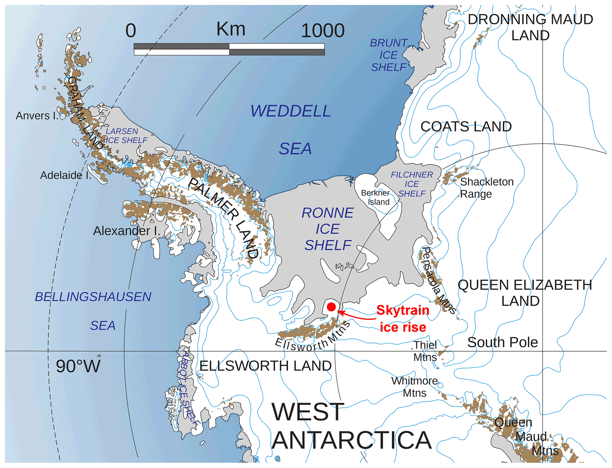
The ice core investigated in this study was drilled as part of the WArm Climate Stability of the West Antarctic ice sheet in the last INterglacial (WACSWAIN) project. This project aims to decipher the, so far unclear, fate of the West Antarctic Ice Sheet (WAIS) and the Filchner–Ronne Ice Shelf (FRIS) during the last interglacial (LIG), which was the last natural warm period, ∼120 000 years before present. For this purpose, an ice core was drilled at Skytrain Ice Rise (Fig. 1), a location that is adjacent to both WAIS and FRIS but that, according to modelling studies (DeConto and Pollard, 2016), likely remained ice-covered during the LIG. Here we present the first part of a chronology for the Skytrain ice core. We focus on the last 2000 years contained in the top 200 m and use a combined approach of annual layer counting and the identification of absolute age markers, namely the tritium peak and volcanic eruptions. High-resolution methane data are used to further support and verify the chronology. This depth–age relationship for the last 2000 years will be used to constrain a chronology of the deeper part of the core, which is discussed in our companion paper (Mulvaney et al., 2022) that is currently in preparation.

2 Methods

2.1 The WACSWAIN ice core

The drilling site (79^∘44.46^′ S, 78^∘32.69^′ W) for the ice core at Skytrain ice rise in West Antarctica was selected based on initial ground-penetrating radar exploration that showed a well-pronounced Raymond arch and undisturbed layering within the study area (Mulvaney et al., 2021). The mean annual surface air temperature at the site is −26 ^∘C, so no substantial influence of surface melt was expected. The surface elevation at the drilling site is 784 m above sea level (a.s.l.). The core was drilled to bedrock during the 2018/19 field season and has a total length of 651 m. Each 80 cm core piece was weighed to calculate density. The depth of bubble close-off, determined by high-resolution discrete total air content analysis, was reached at 58 m total core depth. Dielectric profiling (DEP) measurements (Wilhelms et al., 1998) were carried out on each core piece before processing.

Figure 1 Map of West Antarctica and the Ronne Ice Shelf (modified from USGS, 1999) showing the drilling site (arrow) of the ice core drilled on Skytrain Ice Rise.

2.2 Continuous flow analysis

Chemical analyses of the Skytrain ice core were carried out at the British Antarctic Survey (BAS) in Cambridge via continuous flow analysis (CFA). This setup comprises an inductively coupled plasma mass spectrometer (ICP-MS) for ²³Na, ²⁴Mg, ²⁷Al, ⁴³Ca, and ⁴⁴Ca; two fast ion chromatography (FIC) systems for anion and cation analysis; a particle counter; a fluorescence detection setup for H₂O₂, NH${}_{\mathrm{4}}^{+}$, and Ca²⁺; and two conductivity meters and two Picarro spectrometers – one for online stable water isotope analysis and one for methane concentration analysis (Grieman et al., 2021). An overview of the instruments and their specifications is given in Table 1.

Table 1 Overview of the instrument specifications used in the continuous flow analysis of the Skytrain ice core. The values given for depth resolution of the ICP-MS, FIC and fluorescence instruments were determined in Grieman et al. (2021). The other values were estimated during the Skytrain CFA measurement campaign. The term “Depth resolution” refers to the minimal depth interval (layer thickness) that can be resolved by the respective method. The column “Points per millimetre” refers to the number of data points recorded per millimetre of ice core at an average melt speed for the respective instrument throughout the last 2000 years.

A schematic of the entire CFA setup is given in Fig. 2. Longitudinal CFA sticks of 3.2 cm × 3.2 cm × 80 cm were cut from the whole length of the ice core using a band saw in a cold room. The ends of each stick and every break surface were scraped before melting to reduce contamination. The sticks were continuously melted at a speed of about 3.5–4 cm min⁻¹ in the firn section, ∼ 3 cm min⁻¹ for the middle section of the core and ∼1.6 cm min⁻¹ for the basal 100 m. The electrically heated melt head consists of five meltwater lines, four outer and one inner, of which only the central one was used for analysis (see also Fig. 2). The whole length of the core was analysed. Calibration of the ICP-MS, FICs, fluorescence and water isotope instrument was performed at the beginning and the end of each measurement day using standard solutions of known chemical and isotopic composition. Further information on limits of detection, sensitivity and the standardisation process can be found in Grieman et al. (2021).

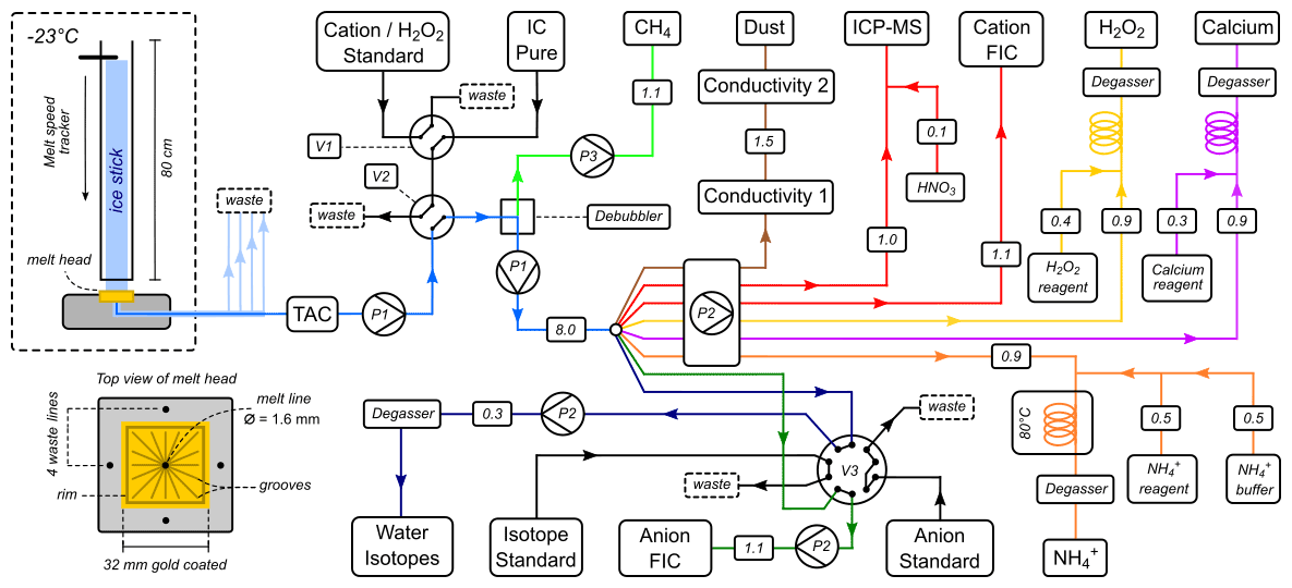
Figure 2 Schematic of the CFA setup at the BAS ice core analysis lab. The meltwater from the inner part of the core is distributed to 12 different analytical systems. The small numbers on the lines denote meltwater flow rates in millilitre per minute.

Both FIC systems for cation and anion analysis were run in parallel, sampling from the same core depth interval. Both FICs consist of two internal measurement systems. They use a dual column system. Each of the two 1.0 mL sample loops was loaded sequentially from the continuous meltwater stream at a flow rate slightly above 1.0 mL min⁻¹. For the anion detection, a Dionex ICS-6000 fast ion chromatography (FIC) system with conductivity detection was used. The sample was separated using Dionex AS15 (5 µm, 3×150 mm) columns and a 60 mM NaOH eluent. A similar approach for anion detection has been used in the field (Schüpbach et al., 2018). Details about the cation system can be found in Grieman et al. (2021). The depth resolution of the ICP-MS analysis is a running average of about 4 cm for Na, Mg and Ca. The depth resolution of the fluorescence calcium detection was found to be ∼1.4 cm. The FIC instruments have a theoretical depth resolution of about 4 cm, but one sample was measured every 2.63 cm (Grieman et al., 2021) and not continuously. At this resolution, an annual layer thickness of at least 5 cm was estimated to be distinguishable using the ICP-MS method. The fluorescence calcium detection method was estimated to be able to detect layers with a minimum thickness of 2 cm. These depths resolutions, meaning the capability of the respective system to resolve layers down to a certain thickness, are mainly dominated by smoothing effects in the tubing and the interfaces and not by the measurement capabilities of the instruments themselves (see Table 1, column “Points per millimetre”). The depth assignment of each dataset was calculated by combining the melt speed, measured by vertical dislocation of the encoder on top of the melting stick, the flow rates and the measured time delays from the melt head to the respective instruments. The top and bottom depth measured for each core piece during the cutting of the core were used as depth assignment boundaries, so there are no propagating depth errors with increasing core depth. The time at which each break in the ice core reached the melt head was manually recorded in Labview by the system operator. Time delays for each instrument were then added to these recorded times to determine instrument analysis times for each ice core break depth. The melt rate was used to adjust ice core depths assigned to instrument analysis times between each break. If this melt rate correction resulted in depth assignments deeper than the depth of the following break or if the melt rate was not recorded, then an evenly spaced depth scale was applied between ice core breaks.

To determine time delays between the melt head and the instruments, the liquid conductivity data on a depth scale estimated using no time delay was compared to DEP data at the same depths for each CFA measurement day; because DEP was measured directly on the solid core, its depth is assumed to be correct. First the depth scale of the liquid conductivity was assigned using the variable melt speed readout from the decoder as described above. Any unexpected spikes in this recorded melt rate were removed by interpolation. The MATLAB “xcorr” function was then used to estimate a depth “lag” between the two datasets for each CFA day. This depth lag is an estimate of the time delay between the melt head and the conductivity detectors. The depth assignments of the liquid conductivity, dust and fluorescence Ca²⁺ measurements were corrected using this depth lag. The ICP-MS calcium data on an instrument analysis timescale for each CFA measurement day were then compared to the raw fluorescence Ca²⁺ data. The xcorr function was used to estimate the analysis time delay between the fluorescence Ca²⁺ measurements and the ICP-MS calcium measurements. The sum of this time delay and the time delay calculated for the depth shift of the calcium fluorescence data was used to shift the instrument analysis time of the ICP-MS and cation and anion FIC raw data before applying the depth scale to the raw data.

2.3 Absolute age markers

2.3.1 Tritium analysis

Every chronology of an environmental archive established using relative stratigraphic counting techniques requires absolute age markers to verify the counted age over depth and to evaluate the corresponding age uncertainty. Vast amounts of anthropogenic tritium (³H) were injected into the atmosphere by thermonuclear explosions from the late 1950s until the partial test ban treaty became effective in 1963 CE, with some tests continuing after that. This tritium emission has been reported to be globally distributed and was found in Antarctic snow samples (Taylor, 1964), where it still could be detected 15 years ago (Fourré et al., 2006). Twenty firn samples between 10.4 and 18.95 m depth were selected for tritium analysis. This depth range was chosen based on a first estimation of the accumulation rate from seasonal variations in the water isotope signal of snow pit samples from the drilling site and the initial annual layer counting using the sodium ICP-MS signal. The ³H content of the meltwater was measured at the Federal Institute of Hydrology in Koblenz, Germany (sample data in Table A1). The samples were distilled, and tritium was electrolytically enriched. The tritium concentration was measured by low background liquid scintillation counting (Quantulus GCT 6220) with a detection limit of about 0.7 TU (Schmidt et al., 2020) .

Tritium concentrations were found to be very low (<12 TU) but measurable. The results are shown in Fig. 3, along with tritium concentrations that were measured in precipitation at Invercargill (NZ) and in a snow pit at Vostok station (Antarctica) in 2008 (Fourré et al., 2018). The peak of the Skytrain tritium concentration (10.92 TU) was visually matched with the peak concentrations in the precipitation data. Based on this visual comparison, the year 1965 CE was identified at a depth of 7.2 m w.e. in the Skytrain ice core. As an important result, the near-surface accumulation rate could be derived to be 13.5 cm w.e. yr⁻¹.

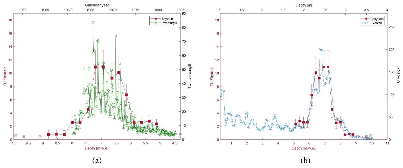
Figure 3 Tritium analysis of the Skytrain ice core (red squares) compared to (a) Invercargill precipitation concentration (green circles) and (b) snow pit data from Vostok station (Antarctica) (blue circles) (Fourré et al., 2018). The samples denoted by open squares were below the detection limit (<0.7 TU).

2.3.2 Volcanic eruptions

One of the most commonly used age markers in ice cores are the chemical and physical signatures of well-dated, global or hemispheric volcanic eruptions (Sigl et al., 2015). These eruptions can be identified as peaks in acidity from the DEP signal or in the non-sea-salt sulfate concentration (Castellano et al., 2005). On the East Antarctic plateau, these volcanic signatures are very distinct and are visible as clear peaks above the background sulfate concentration (Baroni et al., 2008). However, the geographic location in West Antarctica and the comparably low elevation of the Skytrain ice core mean that this site is much more influenced by marine air masses with large inputs of marine biogenic and sea-salt sulfate (e.g. Dixon et al., 2004). This difference is also confirmed by two nearby ice cores from the Antarctic Peninsula, where high background biogenic sulfate overwhelms the volcanic signal (Emanuelsson et al., 2022). As such, the Skytrain ice core shows high and variable sulfate levels, and it is not possible to definitively identify volcanic eruptions from the DEP or CFA data. This issue has also been reported for other near-coastal ice core sites and can restrict the use of volcanic tie points in stratigraphic age models (Philippe et al., 2016; Winstrup et al., 2019).

Therefore, this study used a new method to identify volcanic eruptions from the sulfur (S) isotope composition of sulfate (from now on denoted as ${\mathrm{SO}}_{\mathrm{4}}^{\mathrm{2}-}$) in the ice. Volcanic S emissions have been shown to have distinctive, isotopically light values compared to other dominant inputs from sea-salt or marine biogenic ${\mathrm{SO}}_{\mathrm{4}}^{\mathrm{2}-}$ (Rees et al., 1978; Nielsen et al., 1991; Patris et al., 2000), meaning that S isotope analyses can be used to determine which ${\mathrm{SO}}_{\mathrm{4}}^{\mathrm{2}-}$ peaks have a volcanic origin and define the precise depth of volcanic tie points. Sulfur (S) isotope analyses were conducted at the Department of Earth Sciences at the University of Cambridge Isotope Group clean laboratories using a Thermo Scientific Neptune Plus™ multi-collector inductively coupled mass spectrometer (MC-ICP-MS). Potential depth intervals for volcanic eruption identification were selected based on the depth of the tritium peak, the initial layer counting and the identification of peaks in ${\mathrm{SO}}_{\mathrm{4}}^{\mathrm{2}-}$ from the CFA data. The ice was cut into 5–7 cm length sections and scraped with a razor blade to remove potential surface contaminants. After melting, an aliquot of these samples was measured for discrete ${\mathrm{SO}}_{\mathrm{4}}^{\mathrm{2}-}$ concentrations on the IC (ion chromatograph), and then the volume needed to target 30 nmol of ${\mathrm{SO}}_{\mathrm{4}}^{\mathrm{2}-}$ was transferred to acid-clean Teflon vials and evaporated to dryness at 80 ^∘C. The samples were resuspended in 70 µL of ultra-pure water (resistivity >18 MΩ cm) and passed through anion-exchange columns following methods adapted from Burke et al. (2019) to separate the ${\mathrm{SO}}_{\mathrm{4}}^{\mathrm{2}-}$ from other components in the ice.

All measurements on the MC-ICP-MS were made in high-resolution mode, using an Aridus introduction system. We used standard-sample bracketing protocols with Na₂SO₄ to account for mass bias and instrumental drift following the method developed by Paris et al. (2013). Sulfur isotope compositions were reported using δ^xS notation, as the difference of either the ${}^{\mathrm{34}}\mathrm{S}{/}^{\mathrm{32}}\mathrm{S}$ or ${}^{\mathrm{33}}\mathrm{S}{/}^{\mathrm{32}}\mathrm{S}$ ratio of each sample from the Vienna-Canyon Diablo Troilite (VCDT) in parts per mille (‰) (Eq. 1).

$$\begin{array}{}\text{(1)}& {\mathit{\delta }}^x\mathrm{S}={\displaystyle \frac{{\left({\mathit{\delta }}^x\mathrm{S}/{\mathit{\delta }}^{\mathrm{32}}\mathrm{S}\right)}_{\mathrm{sample}}}{{\left({\mathit{\delta }}^x\mathrm{S}/{\mathit{\delta }}^{\mathrm{32}}\mathrm{S}\right)}_{\mathrm{standard}}}}-\mathrm{1}\end{array}$$

The relative deviation between the δ³³S and δ³⁴S ratios was calculated using Δ³³S notation (Eq. 2), where values outside an analytical error of zero indicate mass-independent fractionation (Farquhar et al., 2001). Mass-independent fractionation of S occurs when sulfur dioxide is photo-oxidised to ${\mathrm{SO}}_{\mathrm{4}}^{\mathrm{2}-}$ by short-wave UV radiation above the ozone layer (Savarino et al., 2003), meaning that non-zero Δ³³S values can be used as a marker of stratospheric volcanic eruptions (Gautier et al., 2019; Burke et al., 2019).

$$\begin{array}{}\text{(2)}& {\mathrm{\Delta }}^{\mathrm{33}}\mathrm{S}={\mathit{\delta }}^{\mathrm{33}}\mathrm{S}-\left(({\mathit{\delta }}^{\mathrm{34}}\mathrm{S}+\mathrm{1}{)}^{\mathrm{0.515}}-\mathrm{1}\right)\end{array}$$

All samples were measured at least in triplicate. Long-term reproducibility was quantified by repeated measurements of an H₂SO₄ ICP-MS standard (${\mathit{\delta }}^{\mathrm{34}}\mathrm{S}=+\mathrm{3.13}$ ‰, σ=0.06, n=26) and IAPSO seawater (${\mathit{\delta }}^{\mathrm{34}}\mathrm{S}=+\mathrm{21.18}$ ‰, σ=0.09, n=26), which showed good agreement to published values from multiple previous studies (Craddock et al., 2008; Das et al., 2012). Conservative errors of ±0.20 ‰ and ±0.15 ‰ were assigned to all δ³⁴S and Δ³³S values, respectively, equalling ±2σ variability of repeat measurements of standards and replicate samples.

These analyses allowed for a clear distinction between background and volcanic S isotope compositions and the identification of the exact depth interval of well-dated volcanic eruptions. The samples interpreted to reflect background conditions had δ³⁴S values ranging from +15.86 to +18.76 ‰ (mean $=+\mathrm{17.43}$ ‰), and the samples defined as volcanic had values ranging from −12.31 to +14.32 ‰ (mean $=+\mathrm{5.64}$ ‰). Many of the volcanic samples also showed mass-independent fractionation (range ${\mathrm{\Delta }}^{\mathrm{33}}\mathrm{S}=-\mathrm{1.36}$ to +0.93 ‰), whereas all background Δ³³S values were within an analytical error of zero, giving additional evidence to define the depth of stratospheric volcanic eruptions.

A total of 43 samples were analysed, and seven volcanic events were identified (Table B1), corresponding to the 1815 CE eruption of Tambora; the 1458 CE eruption of Kuwae; and four eruptions at 1285, 1276, 1257 and 1229 CE from the Samalas sequence (Sigl et al., 2015). A peak potentially representing an eruption of unknown origin in 1110 CE was also identified. Examples of the peak selection for volcanic tie points are shown in Fig. 4.

Figure 4 Examples of the depth selection for δ³⁴S sampling for identification of volcanic eruptions based on DEP (density corrected, top), FIC sulfate (middle) and CFA liquid conductivity (bottom) signals. Panel (a) shows the peaks selected for identification of the 1815 CE Tambora eruption, panel (b) shows the peaks selected for identification of the 1458 CE eruption, panel (c) shows the peaks selected for identification of the 1257 CE eruption sequence of four (1229, 1257, 1276 and 1285 CE) and panel (d) shows the peaks selected for identification of a potential 1110 CE eruption. The green bars denote the samples that had volcanic S isotope compositions. The grey bars denote other samples that were analysed in the search for the respective eruption but that had background S isotopic compositions.

2.3.3 Methane measurements

To further constrain the layer-counted chronology below the depth of the deepest confidently identified volcanic eruption (1229 CE, 97.45 m), we measured methane concentrations in the Skytrain ice core and compared them to the high-resolution WAIS Divide ice core methane dataset (Mitchell et al., 2011; Köhler et al., 2017). In total, 39 discrete Skytrain ice core samples from the archive piece (quarter core) were selected at 1.5–1.6 m depth intervals between 84 and 143.20 m, working around any cracks and breaks to achieve the best ice quality for gas analysis. This depth interval overlaps with the presumed depth of the 1257 CE volcanic eruption sequence.

The samples were analysed at Oregon State University (USA) using a melt and refreeze wet-extraction technique as described in detail in Grachev et al. (2009), Mitchell et al. (2011) and Lee et al. (2020). In brief, samples of approximately $\mathrm{10}\times \mathrm{3}\times \mathrm{3}$ cm (long side orientated vertically along the core) were sealed in individual glass vacuum flasks and attached to the extraction line. The extraction procedure is automated to give exact replication of the method for each sample. The samples are firstly kept frozen in an ethanol bath while evacuating the flasks to vacuum. A warm water bath then melts the samples, releasing the trapped air into the headspace above the meltwater. Refreezing of the samples, again in an ethanol bath, precedes expansion of the extracted air into a gas chromatograph (GC) for measurement of the CH₄ concentration. Expansion is repeated four times per sample. All concentrations were referenced to the WMO X2004A reference scale (Dlugokencky et al., 2005) and were calibrated using a NOAA primary air standard with a calibrated concentration of 481.25 ppb CH₄. Final concentrations were corrected by subtraction of an average background value of 8.25 ppb, determined by expanding the air standard over gas-free ice samples that are measured using the same procedure as described above. A solubility correction accounts for the small portion of air that remains dissolved in the meltwater and is therefore not extracted, following the derivation in Mitchell et al. (2013). A total of 1 ppb was added to each sample to account for the solubility, giving the final CH₄ value.

Two true-depth replicate samples are usually measured in this method. However, available ice resulted in only one sample of large enough volume for the required methodology. As a result, one measurement per depth level is presented here. Given the strong validation of the method in previous studies, the requirement for only matching overall CH₄ trends as opposed to absolute values of CH₄ for this dating purpose, and the good correspondence of the trends observed in the Skytrain CH₄ in comparison to the WAIS record, this is determined to be satisfactory. The overall uncertainty of the CH₄ data presented here is estimated to be 2–3 ppb, based on errors of previous studies using the same analytical system where duplicate measurements were available (Mitchell et al., 2011, 2013; Epifanio et al., 2020).

Additionally, methane concentrations were analysed continuously in a 17 m long ice core section (144–161 m) adjoining the discrete sample section on the deeper end using the BAS CFA system and a Picarro G2301 CRDS instrument. Similar to the CH₄ dissolution effect described for the discrete CH₄ data, the continuously measured data are always lower than the actual atmospheric value because a small amount of air dissolves in the meltwater on its way to a hydrophobic membrane module (Fig. 2). Absolute values of this highly resolved continuous data are typically assigned using a few discretely measured CH₄ anchor points. We do not have any discrete CH₄ data for the depth section that was measured in a continuous fashion. Therefore, we calibrated the instrument's output by measuring NOAA primary air standards (405.8 ppb and 869.1 ppb CH₄ calibrated against the WMO X2004A reference scale, Dlugokencky et al., 2005) and checked for linearity (R²=0.998) using a working gas standard (602.0 ppb). We then made daily calibrations mimicking gas extraction from meltwater through a full loop using degassed deionised water and the working gas standard. Therefore, CH₄ values were calibrated to the NOAA scale using a slope of 0.970 and an intercept of −6.278. We estimated the dissolution factor to increase the raw measurements by 8.73 %. The instrumental CFA CH₄ uncertainty is 10 ppb.

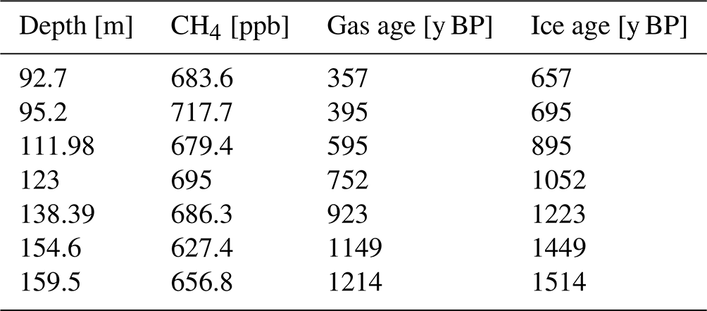
The combined discrete and continuous methane concentrations from 84 to 161 m were then matched to the high-resolution CH₄ data from the WAIS Divide ice core (Fig. 5). The variations of the WAIS CH₄ record on the gas age scale were visually aligned with the Skytrain CH₄ on its depth scale. Seven tie points were manually identified (Table C1) and are shown by the dashed lines in Fig. 5. Subsequently the WAIS Divide ice core gas age (WD2014, Sigl et al., 2019) was assigned to the corresponding Skytrain ice core depth. To determine the gas-age–ice-age difference (delta age), the age difference between the derived Skytrain ice core gas ages and the matching volcanic tie point ice ages in the depth interval between 84 and 98 m was calculated . This delta age was found to be about 300 years. The delta age was then added to all the matched gas ages to convert them into the respective ice ages. Please note that it is beyond the scope of this paper to establish and analyse the full gas age chronology of Skytrain ice core. Here the methane data were used to support the annual-layer-counted ice age chronology. The full gas age scale based on CFA methane measurements will be addressed in the companion paper.

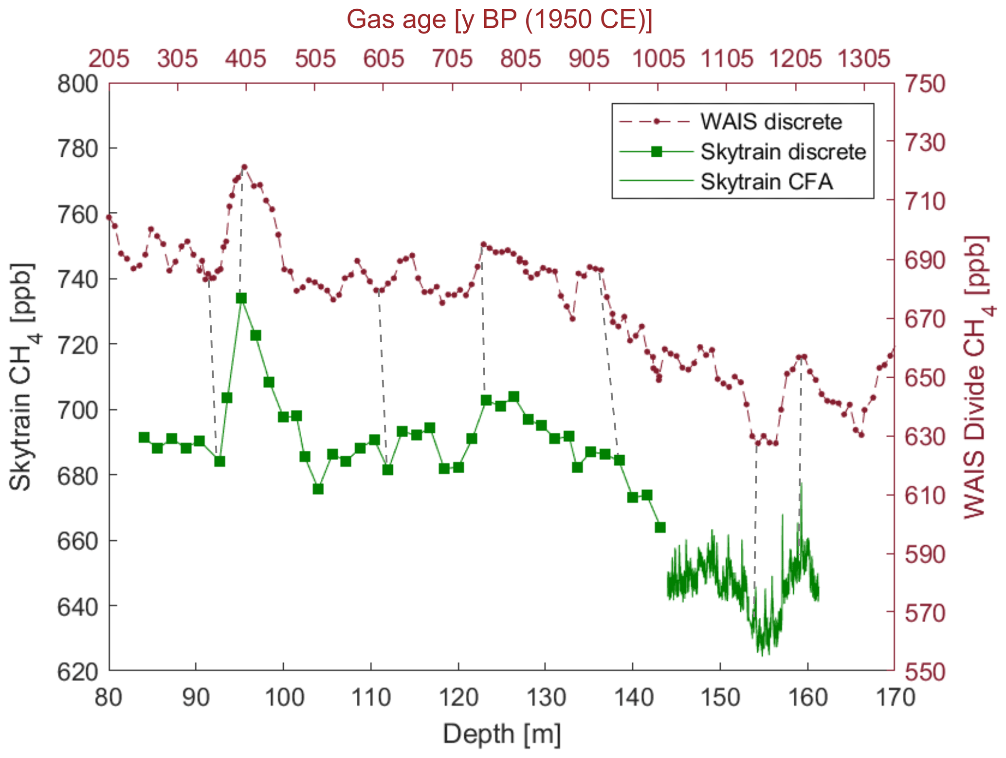
Figure 5 Skytrain methane measurements compared to WAIS Divide ice core methane measurements (Mitchell et al., 2011). The green squares denote discrete Skytrain methane measurements completed at Oregon State University. The green line shows the continuous methane concentrations analysed using the BAS CFA system. The Skytrain ice core methane record on a depth scale was compared visually to best fit the variability of the WAIS record on its age scale (WD2014) (Sigl et al., 2019). The “y BP” abbreviation denotes years before present (1950 CE). The selected tie points are marked by the grey dashed lines connecting the shown records.

3 Core chronology

3.1 Layer identification

3.1.1 Manual identification

It should be noted that the layer identification in the Skytrain ice core was generally challenging, mainly because of the high noise and (marine) background levels of the respective species. This is a feature of the site and not caused by the analytical methods. We therefore would like to emphasise that the annual layer counting only serves as an interpolation between the absolute age markers and does not stand as a chronology alone. Annual layers were identified using chemical species that are known to show seasonal variations in concentration. Because of the comparably high and variable (mainly marine) background of many chemical species (e.g. sulfate) in the Skytrain ice core, it was not sensible to apply automated layer identification algorithms like StratiCounter (Winstrup et al., 2012). Instead, the counting was performed manually using Matchmaker, a graphical MATLAB application, which allows annual layer counting of multiple records simultaneously (Rasmussen et al., 2008). Some of the most common parameters used to investigate seasonal variations and to identify annual layers in the firn section of Antarctic ice cores are the H₂O₂ concentration and stable water isotope ratios (Schlosser and Oerter, 2002; Sigg and Neftel, 1988). However, in the Skytrain ice core, these parameters only show a seasonal cycle in the top 10–15 m of the core. Below 15 m, both signals become too smoothed to resolve annual variability. Sodium and MSA (methanesulfonic acid) also commonly show seasonal variability in Antarctic ice cores. Sodium concentrations peak in the austral winter layer, due to the combined influence of sea ice emissions and increased transport, and MSA peaks in the austral summer due to enhanced biological activity (e.g. Sigl et al., 2016; Osman et al., 2017). In the Skytrain ice core, MSA peaks at the same time as sodium. This phenomenon of migration into winter snow layers has been observed perviously (Pasteur and Mulvaney, 2000). Conversely, sulfate concentrations are highest in the austral summer (Preunkert et al., 2008). Therefore, minima in the ${\mathrm{SO}}_{\mathrm{4}}^{\mathrm{2}-}/\mathrm{Na}$ ratio coincide with maxima in sodium and MSA and are used in this study to underpin the identification of annual layers. Examples of Na (ICP-MS), MSA (FIC) and ${\mathrm{SO}}_{\mathrm{4}}^{\mathrm{2}-}$ (FIC) $/$ Na data along with calcium concentrations from fluorescence detection at the same depths are shown in Fig. 6. Another parameter which is known to show seasonal variations in coastal Antarctic sites is nitrate (Wagenbach et al., 1988). However, this parameter was also measured using the FIC system and did not have an advantage in terms of depth resolution compared to the MSA. Measured intensities were low, and therefore this component was not considered as an annual marker.

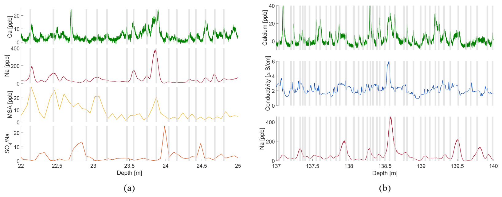
Figure 6 Skytrain ice core chemical records from (a) 15–18 m (∼ 1952–1961 CE) and (b) 140–143 m (∼ 713–752 CE). Above ∼70 m, annual layers were identified by common peaks in Na (ICP-MS signal) and MSA (FIC signal) along with minima in ${\mathrm{SO}}_{\mathrm{4}}^{\mathrm{2}-}$ (FIC) $/$ Na ratios. Below ∼70 m, calcium concentrations were used as the primary annual layer indicator. The grey bars denote the identified annual layers.

The proposed relationship between the markers described above is clearly visible in the data. In particular, parallel annual variations in MSA and Na concentrations are distinct. This variability strongly suggests that the measured sodium signal is showing seasonal variability. Sodium was therefore used as the primary indicator for annual layer counting of the top ∼ 60–70 m. Below ∼ 60–70 m, annual layers in the MSA and ${\mathrm{SO}}_{\mathrm{4}}^{\mathrm{2}-}/\mathrm{Na}$ signals could no longer be identified due to the limited depth resolution of the FIC method. The sodium-derived depth–age relationship also became linear below ∼70 m and no longer followed the exponential shape expected due to thinning. This linearity is due to the limited depth resolution of the ICP-MS measurements. However, Fig. 6a shows that there is a strong correlation between the higher-resolution fluorescence calcium signal and the sodium signal, which has also been observed in other Antarctic ice core records (e.g. Curran et al., 1998). Based on this finding, below ∼ 60–70 m, calcium was used as the primary indicator for seasonal variations, in combination with sodium and liquid conductivity (Fig. 6b). The aim was to achieve a gradual transition between the primary markers by attempting to slowly include more peaks from the calcium signal into the sodium count until the calcium record became the primary seasonal indicator. Therefore, an exact depth for the shift to calcium as the primary indicator cannot be given. Below a depth of ∼200 m, the depth–age relationship of the calcium signal also became linear, which suggests that the limit of the fluorescence calcium depth resolution (1.4 cm) was reached. Further counting would only have resulted in an increasing and hard to determine age uncertainty.

3.1.2 Power spectra

To support our findings of the manual layer identification, similar to the approach in Bigler et al. (2011) we calculated simple power spectra for the most important components (Na, Ca, MSA and conductivity) in two different depth intervals (Fig. 7).

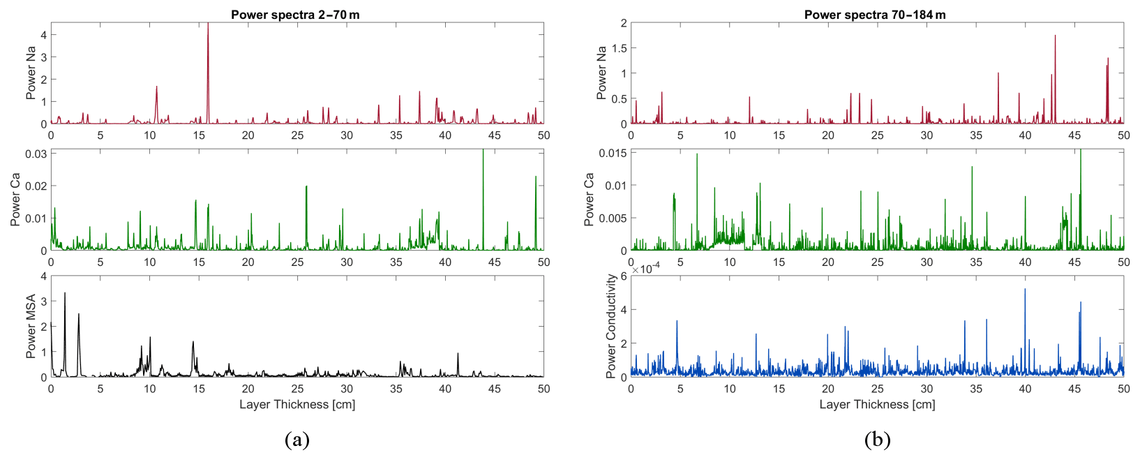
Figure 7 Power spectra for Na, Ca, MSA and conductivity for two different depth intervals. Panel (a) shows the shallow part of the core (0–70 m) and panel (b) the deeper part (70–184 m). In the shallow part, clear peaks in the sodium and the MSA data around 10 and 15 cm are visible. In the deep part, some variations around 40–45 cm layer thickness are dominant, but also a distinct maximum in the Ca data between 4 and 12 cm layer thickness is visible.

In the shallow part, the sodium and MSA power spectra show clear maxima around 10–15 cm layer thickness, which is in good agreement with the findings from the manual layer identification. In addition, the calcium data show enhanced values around 10–15 cm but less distinct. The two large peaks in the MSA data between 2 and 3 cm must be attributed to noise in the measurement and cannot refer to actual layers. In the deeper part of the core, the maxima in the power spectra are less obvious, mainly due to the expected higher noise level. There is a clear rather wide maximum in the Ca record between about 4 and 12 cm layer thickness, which corresponds well to the layer thicknesses that have been identified manually in this depth section (see also Fig. 9). In addition, in the conductivity record there is a small maximum around 5 cm layer thickness, matching the findings from the manual layer counting. Remarkably, all records of Na, Ca and liquid conductivity show rather pronounced maxima between about 40–45 cm layer thickness. These variations might hint to some decadal variations. An in-depth discussion of these features is, however, beyond the scope of this study.

3.2 Strategy for integration of absolute age markers and layer counting

The absolute age markers, including the date of the tritium peak, the volcanic eruptions, and the methane measurements, were regarded as intermediate reference points in the layer counting procedure. While the depth of the tritium peak and the positions of the volcanic eruptions were considered to be robust with a small age error (<1 year), the methane reference points are less well defined, mainly because of the uncertainties in the assumed delta age of the gas record. Above 13.5 m, the depth of the 1965 CE tritium peak was used as a fixed starting point to calibrate the layer identification procedure. In the first test, the counting was performed using the Na, MSA and ${\mathrm{SO}}_{\mathrm{4}}^{\mathrm{2}-}/\mathrm{Na}$ ratios as described above. The deviation from 1965 CE in the initial counting attempt was roughly 10 %. In a second counting run, the layer counting was adjusted to fit the position of the 1965 CE peak to 1 year. The same strategy was subsequently applied to fit the dates of volcanic eruptions. For this deeper part below 13.5 m, initial calibration of the layer count was performed between the well-defined depths of the 1285, 1257 and 1229 CE volcanic eruptions. Peak identification in this section mainly relied on the calcium fluorescence and the conductivity signals. After these two initial tunings of the counting procedure, layer counting below 13.5 m was continued back in time to meet the 1815 CE Tambora eruption depth and consecutively further to 1458 CE. As explained in Sect. 3.1, at a depth between about 60–70 m, variations in the Na, MSA and ${\mathrm{SO}}_{\mathrm{4}}^{\mathrm{2}-}/\mathrm{Na}$ ratios no longer resolve annual cycles. Therefore, a gradual transition to incorporate more layers visible in the higher-resolution calcium data was implemented. To confirm this transition, the time frame between 1285 and 1815 CE was also counted forward in time to assess the uncertainty in the chronology when transiting from high-resolution to low-resolution data. It should be noted that in the layer counting procedure, the depths of the 1965, 1285, 1257 and 1229 CE tie points were considered to be fixed within 1 year, whereas the depth of the 1458 CE eruption was not. This difference is mainly due to the fact that around the 1458 CE depth the peak identification method switched from the sodium- to calcium-dominated approach, leading to a larger age uncertainty in that depth interval. Only the calcium and conductivity records were used for annual layer counting below the depth of the 1229 CE eruption to 2000 years BP. At this depth, annual layers were no longer resolved. The annual-layer-counted chronology, including all age marker tie points, is shown in Fig. 9.

3.3 Investigation of seasonality

To better assess and quantify the seasonality in the signals of the most important chemical and physical markers (Na, Ca, Mg, MSA, ${\mathrm{SO}}_{\mathrm{4}}^{\mathrm{2}-}$ and conductivity), a more detailed investigation of the annual variations has been carried out similar to the procedure used by Winski et al. (2019). First, the CFA records within the annual intervals defined by the counting markers were interpolated over a 12-month period. Then, the CFA signals for the respective species were averaged for each month over different depth intervals of the core (0–50, 50–80, 80–115 and 115–184 m). To normalise these mean concentrations and make them comparable, the monthly-averaged signals were subsequently divided by their respective annual mean. The relative deviations from the annual mean in percent are presented in Fig. 8. The horizontal axes show the annual patterns of the signal over 12 months, with zero denoting 1 January. The depth intervals for averaging were chosen based on observations from the layer counting. The first one (0–50 m) mainly relied on the counting of the sodium and MSA peaks, the second on sodium and calcium, and the last two mainly on calcium and conductivity.

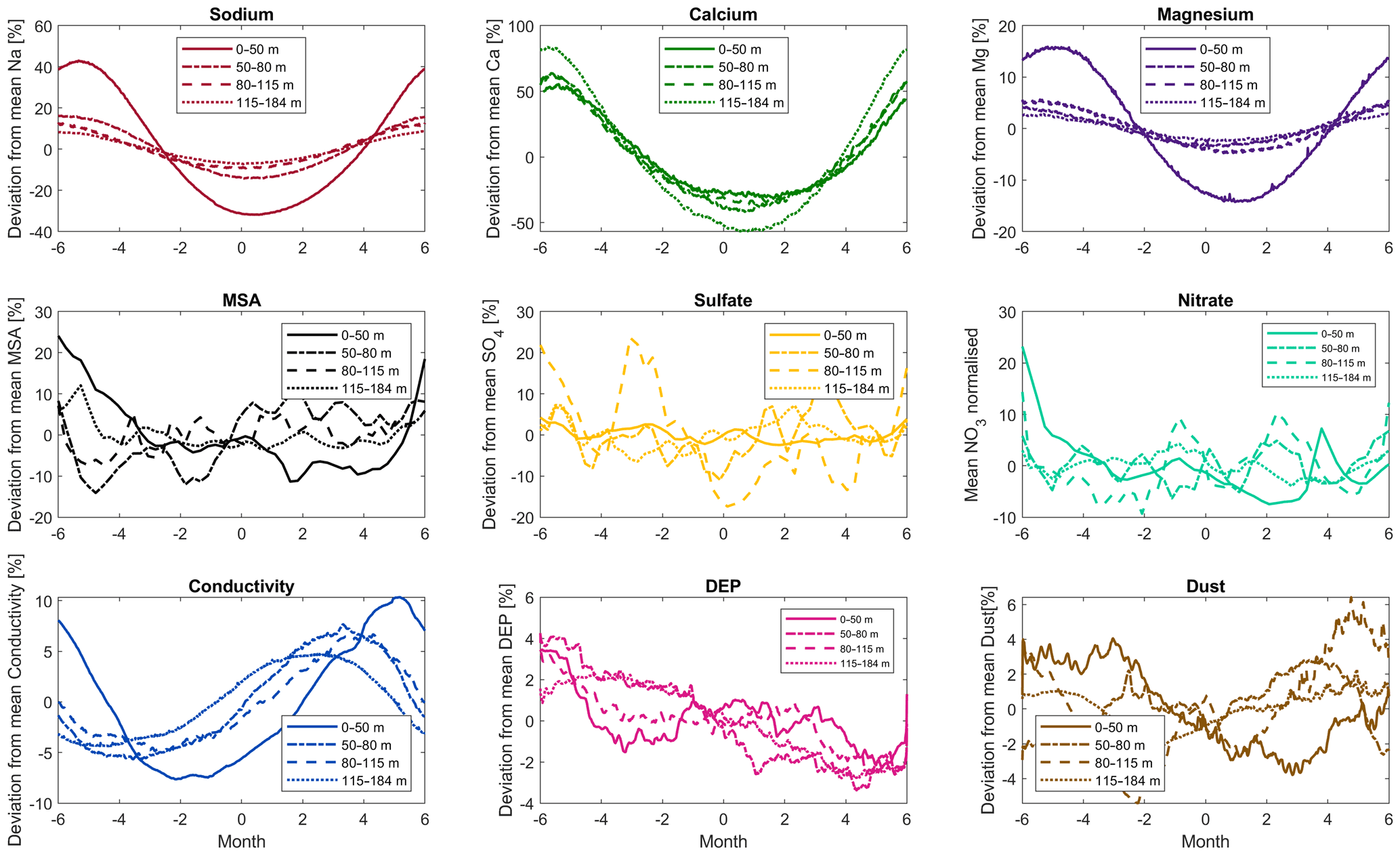
Figure 8 Seasonality analysis of main chemical species from CFA measurements. The horizontal axes show numbered months of the year, with zero denoting 1 January. The vertical axes show the normalised amplitude and the relative deviation from the annual mean of the respective signal for different depth intervals of the Skytrain ice core.

The sodium signal shows the most distinct seasonality in the top 50 m, with maximum values in the Antarctic winter and deviations of more than 40 % from the annual mean. In the deeper sections, the annual cyclicity is much less pronounced. This is due to the fact that sodium was no longer the primary component for layer counting and also to the loss of resolution. Magnesium shows a very similar annual pattern, as expected (Curran et al., 1998), but with a maximum variation of about 15 % from the annual mean that was much less distinct compared to the sodium. Calcium shows the highest amplitude seasonal cycle, with values up to 80 % above the mean in the Antarctic winter. Calcium shows the strongest variation in the lowest investigated core section (115–184 m), which is caused by the fact that it was the main component for annual layer counting in this depth interval. However, the seasonality is also very pronounced in shallower depths, which supports the assumption that the total calcium signal is actually showing annual variations. MSA appears to have a seasonal variation in the top 50 m, where it was also included in the counting scheme. For the deeper parts, the MSA signal varies around the mean and no longer shows a cyclic trend. This result is mainly due to the very limited depth resolution of the FIC instrument. The low FIC resolution also affects the sulfate signal. Similar to the MSA signal, the sulfate also varies randomly around the mean, and no obvious seasonality can be detected. This is also the case for the nitrate signal, which is influenced by the same limitation of depth resolution. The liquid conductivity signal appears to show a seasonal variation with a peak in Antarctic autumn. However, for conductivity the deviation from the mean is only about 5 %, which is very small compared to the other signal variations. A small drift in seasonality is visible, which is most obvious between the top 50 m and the other depth intervals. This drift is very likely caused by the change in layer counting strategy around 60–70 m depth. The DEP signal should be expected to show similar seasonality as the liquid conductivity, but unfortunately these measurements were also done with rather limited depth resolution. Therefore, with this methodological approach, no seasonality in the DEP signal could be detected. The dust signal also does not show a seasonality, which in this case is not caused by limited depth resolution but (unlike some Greenland records for example) by a very noisy dataset.

3.4 Chronology characteristics and the dating uncertainty

The combined approach of annual layer counting and the identification of absolute age markers led to a stratigraphical core chronology for the Skytrain ice core reaching back to 1950±122 years before 1950 CE at 184.14 m total depth (see Fig. 9). In the following, age will be noted as years before present (years BP), with present referring to the year 1950 CE. The average annual layer thickness, also shown in Fig. 9, varies between 0.1 and 0.15 m w.e. in the topmost part of the core to 0.05–0.1 m w.e. below about 90 m depth. There are two phases of accelerated layer thinning that are not related to changes in density (see Fig. 9). The first section is between ∼ 8–15 m total depth (−40 to −5 years BP), and the second is between ∼ 35–46 m total depth (120–200 years BP). We attribute these intervals of thinning, especially the second one, and the overall thinning in the top 90 m to the effects of a distinctive Raymond arch at the drilling site (Raymond, 1983), which has been detected by ground-penetrating radar (Mulvaney et al., 2021). The thinning and more rapid ageing effects of the ice due to this glaciological feature were underestimated in initial age–depth models and only became obvious after identification of the absolute age markers. We cannot rule out that changes in accumulation rate also contribute to the thinner layers.

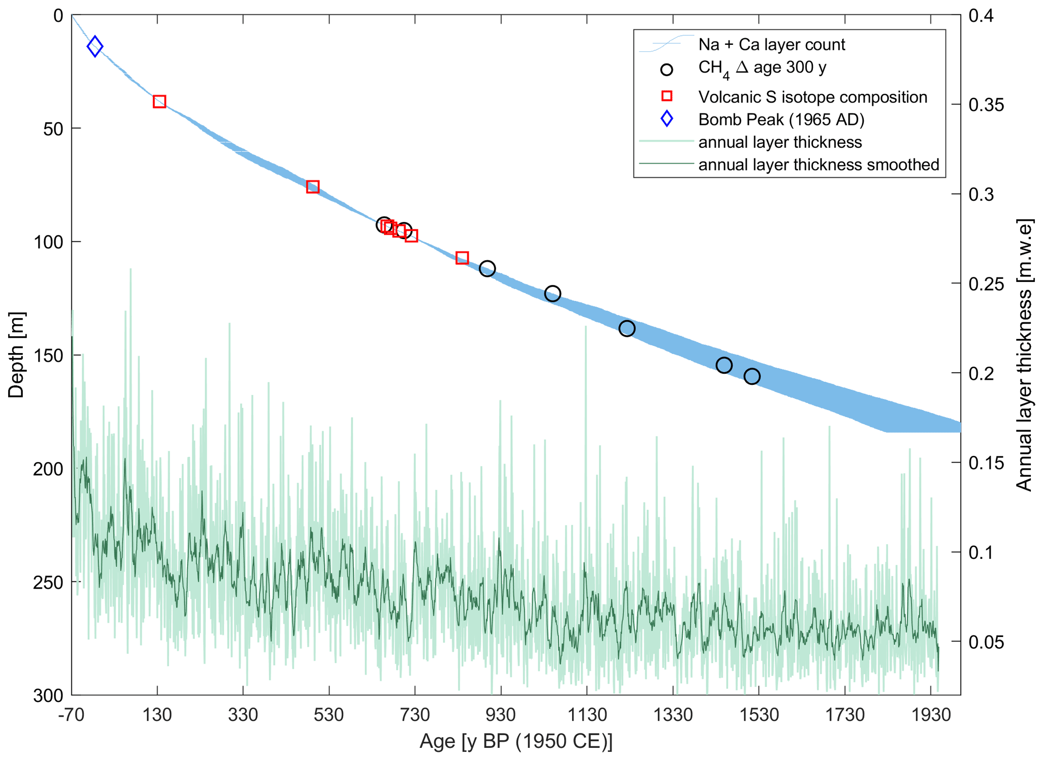
Figure 9 Stratigraphical depth–age relationship of the Skytrain ice core. The blue shaded area shows the annual-layer-counted chronology including the age uncertainty. The blue diamond marks the position of the tritium peak. The squares show the depth of identified volcanic eruptions, and the circles show the methane reference points, assuming a delta age of 300 years. Note that the deepest volcanic eruption date should be considered only as potentially representing the 1110 CE (840 years BP) eruption. The dark green line depicts the 10-year averaged evolution of the annual layer thickness with time; the light green is the unsmoothed layer thickness.

The overall uncertainty of the ice core chronology consists of (i) the uncertainty in identification and counting of annual layers by the operator, (ii) the uncertainty of the depth and age assignment of the tie points and (iii) irregularities in the stratigraphical order (e.g. missing layers). Therefore, a purely mathematical assessment of the error of the derived age–depth relationship is very difficult, and all attempts at quantifying the dating uncertainty must be considered as estimates. By far the largest source of error is missing or overcounting of annual layers by the operator, in combination with the limited resolution of the analytical methods. We tried to minimise these errors by using several independently measured chemical species simultaneously for annual layer counting as described above (see Fig. 6). Based on the findings in Sect. 3.2, we estimated three different counting error ranges for the core sections from 0–38.22 m (the depth of the Tambora eruption), 38.22–93.22 m (the depth of the 1285 CE eruption) and 97.45–184.11 m. These error ranges are shown as the blue shaded area in Fig. 9. For the topmost depth interval a cumulative age error of ±5 % was derived from two iterations of annual layer counting. This error increases with distance from the age markers (here the Tritium peak and the Tambora eruption) and was set to ±1 year at the depths of the tie points. In the second depth interval, the transition from the sodium- to calcium-dominated layer counting was performed. Together with a phase of layer thinning in this section, it was not possible to reduce the counting error to less than ±8 % at the depth of the presumed 1458 CE eruption (75.8 m). Therefore, this volcanic marker was not used as a fixed tie point, and the error range for the whole second depth interval was set to ±8 %. The depth range between the 1285 CE and 1229 CE tie points (93.25–97.45 m) was considered to have an age error of ±1 year because this interval was used to calibrate and tune the counting procedure in the first place. In the deepest section, the error was estimated from the comparison of the counted chronology with the age markers derived from the methane measurements (black circles in Fig. 9). The cumulative error aimed to incorporate all of these age markers in its range, but they were not used as fixed tie points in the chronology. This approach led to an uncertainty range of ±10 % of the respective age in the section between 97.43 and 184.11 m. The highest uncertainty in the lowest section is also justified by the fact that the counting error will increase with depth due to the calcium fluorescence instrument resolution reaching its limitations at layer thicknesses below 5 cm w.e. and the cumulative unconstrained counting error.

4 Conclusions

The first part of the ST22 chronology for Skytrain ice core covering the last 2000 years before present was successfully established. This time period of the most recent past is crucial for understanding current climate change processes, and a well-constrained chronology is a prerequisite for any further data interpretation. An age of 1950 before 1950 CE (BP) was reached at a depth of 184.14 m. The dating of the ice core is based on stratigraphical methods. Annual layer counting has been carried out using primarily the sodium signal as a seasonal indicator in the top ∼ 60–70 m (about 300 years BP) and calcium for the lower part (∼ 60–184 m). The seasonality of the chosen parameters was also supported by power spectra analyses. The annual layer counting was finally constrained to a set of absolute age markers. These age markers include the tritium peak (1965 CE) and six volcanic eruptions identified via sulfur isotope analysis. Methane measurements were used to further verify the counted chronology, although they were not used as fixed age tie points. Based on the depth of the 1965 CE tritium peak, a surface accumulation of 13.5 cm w.e. yr⁻¹ was determined. The overall uncertainty of the record is dominated by counting errors of the operator. A minimum error of ±1 year at the depths of the tie points was assumed. In between the tie points, a cumulative age error of ±5 % in the top part (0–38.22 m), ±8 % in the middle part (38.22–93.22 m) and ±10 % in the unconstrained bottom part (93.22–184 m) was determined. In the lowest part of the investigated core section, a gradual transition to the age model used for the deep ice will be established (Mulvaney et al., 2022). The retrieved depth–age relationship was found to age much faster than expected from initial purely glaciological modelling. At least two phases of enhanced layer thinning at shallow core depths (above 90 m) were observed. This thinning is attributed to the influence of a pronounced Raymond arch. The conservative uncertainty approach allows for interpretations on at least decadal timescales. Overall, the first part of the ST22 chronology provides a robust age scale to interpret climatic signals recorded in the Skytrain ice core during the last 2000 years, as well as for developing the age model for the deeper ice.

Appendix A: Tritium sample data

Table A1 Sample data and results of the tritium measurements in the Skytrain ice core. The deepest five samples were below the detection limit.

Appendix B: Volcanic eruption sulfur isotope data

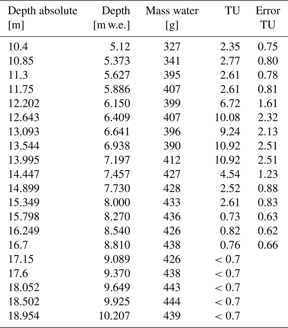
Table B1 Sample data and results of the δ³⁴S and discrete sulfate measurements in the Skytrain ice core. Values are reported in per mille, relative to VCDT. Data of the other samples that were not clearly identified can be found in the Supplement.

Appendix C: Methane age tie points

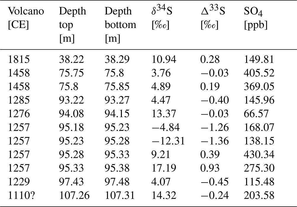
Table C1 Age reference points picked from visual comparison of Skytrain, WAIS Divide and Antarctic composite methane data. A delta age of 300 years was used to convert gas age into ice age for Skytrain ice core. The “y BP” abbreviation denotes years before present (1950 CE).