the Creative Commons Attribution 4.0 License.
the Creative Commons Attribution 4.0 License.
 | 21 Jul 2022
Subdaily meteorological measurements of temperature, direction of the movement of the clouds, and cloud cover in the Late Maunder Minimum by Louis Morin in Paris
Thomas Pliemon
Ulrich Foelsche
Christian Rohr
Christian Pfister
We have digitized three meteorological variables (temperature, direction of the movement of the clouds, and cloud cover) from copies of Louis Morin's original measurements (source: Institute of History/Oeschger Centre for Climate Change Research, University of Bern; Institut de France) and subjected them to quality analysis to make these data available to the scientific community. Our available data cover the period 1665–1713 (temperature beginning in 1676). We compare the early instrumental temperature dataset with statistical methods and proxy data to validate the measurements in terms of inhomogeneities and claim that they are, apart from small inhomogeneities, reliable. The Late Maunder Minimum (LMM) is characterized by cold winters and falls and moderate springs and summers with respect to the reference period of 1961–1990. Winter months show a significantly lower frequency of the westerly direction in the movement of the clouds. This reduction of advection from the ocean leads to a cooling in Paris in winter. The influence of the advection becomes apparent when comparing the last decade of the 17th century (cold) and the first decade of the 18th century (warm). Consequently, the unusually cold winters in the LMM are largely caused by a lower frequency of the westerly direction in the movement of the clouds. An impact analysis reveals that the winter of 1708/09 was a devastating one with respect to consecutive ice days, although other winters are more pronounced (e.g., the winters of 1676/77, 1678/79, 1683/84, 1692/93, 1694/95, and 1696/97) in terms of mean temperature, ice days, cold days, or consecutive cold days. An investigation of the cloud cover data revealed a high discrepancy, with the winter season (DJF, −14.0 %), the spring season (MAM, −20.8 %), the summer season (JJA, −17.9 %), and the fall season (SON, −18.0 %) showing negative anomalies of total cloud cover (TCC) with respect to the 30-year mean of the ERA5 data (1981–2010). Thus, Morin's measurements of temperature and direction of the movement of the clouds seem to be trustworthy, whereas cloud cover in quantitative terms should be taken with caution.
Please read the corrigendum first before continuing.
-
Notice on corrigendum
The requested paper has a corresponding corrigendum published. Please read the corrigendum first before downloading the article.
-
Article
(8396 KB)
-
The requested paper has a corresponding corrigendum published. Please read the corrigendum first before downloading the article.
- Article
(8396 KB) - Full-text XML
- Corrigendum
- BibTeX
- EndNote


The Little Ice Age (LIA, ca. 1300–1850; e.g., Wanner et al., 2000; Grove, 2004; White et al., 2018; Pfister and Wanner, 2021) was one of the coldest periods in the last 2 millennia (Mann et al., 2009). This is based on evidence from proxy records of both hemispheres (Chambers et al., 2014), which suggest that the LIA was a global phenomenon (Rhodes et al., 2012). Nonetheless, the term LIA is controversial and it has been suggested to be abandoned because both the temporal duration and the mean magnitude of the cooling of the LIA are far less pronounced than cold periods, which are named ice ages, and the climate of the LIA was not uniformly cold in space and time (Matthews and Briffa, 2005; Lockwood et al., 2017; Neukom et al., 2019). The Maunder Minimum (MM, 1645–1715) is often regarded as one of the coldest periods of the LIA (Luterbacher et al., 2001; Barriopedro et al., 2008). The coldness reached its climax during the last decades of the MM, which are often called the Late Maunder Minimum (LMM, ca. 1675–1715; Wanner et al., 1995; Slonosky et al., 2001; Legrand and Le Goff, 1987). However, the name Maunder Minimum refers to the study of Walter Maunder called “A prolonged sunspot minimum”, who showed that the sun had little to no sunspots during this time (Lockwood et al., 2017). Thus, the MM (and LMM) is defined to describe a period of very low observed sunspot numbers and is not defined by climatic conditions. Nevertheless, the terminology is meanwhile well established in the climate science community (e.g., Rácz, 1994; Wanner et al., 1995; Alcoforado et al., 2000; Barriendos, 1997; Luterbacher et al., 2000; Xoplaki et al., 2001; Luterbacher et al., 2001; Luterbacher, 2001; Zorita et al., 2004; Zinke et al., 2004; Niedźwiedź, 2010; Barriopedro et al., 2014; Mellado-Cano et al., 2018).
Louis Morin lived from 11 July 1635 to 1 March 1715, and he spent his life in Paris (Legrand and Le Goff, 1987, 1992). He achieved the degree Doctor of Medicine and practiced in Paris. In addition to practicing medicine, he measured different meteorological variables for the time span of 1665–1713 on a daily basis using both early measurement devices and subjective measurements. Therefore, this source can be used to reconstruct the climate during the LMM (Jones, 1999; Pfister, 1999, 2001, 2010). Morin took his measurements in the MM but we will continue with this expression because the majority of his measurements were made in the LMM. The primary focus of earlier studies was on the temperature time series and the pressure time series. For the time period from September 1675 to July 1713, the temperature observations were homogenized and transformed into modern units by Legrand and Le Goff (1987, 1992). The time period from January 1665 to August 1675 was kept untouched due to the coarse divisions of the thermometer (Legrand and Le Goff, 1987, 1992; Legrand et al., 1992). For our analysis, we digitized the three variables that we give attention to from a copy of Morin's original measurements (source: Institute of History/Oeschger Centre for Climate Change Research, University of Bern). We include the original data because we want to make them available to the public. Especially for this paper, an analysis of the validity of the data requires looking at the raw data because applying a transfer function (e.g., for temperature) can cause characteristic details of the time series to be lost.
The temperature time series that we obtained was used to analyze the synoptic atmospheric circulation and the variability, then compare with auroral activities in the 17th century (Legrand et al., 1990, 1992; Diodato et al., 2014). A further correction to the temperature data was made for the time period 1676–1680 (Rousseau, 2013). It was shown that the temperature measurements from 1665 to 1675 are statistically significant on a monthly basis and the period was added to the long-term time series of Paris (Rousseau, 2009). Pfister and Bareiss (1994) investigated temperature, wind direction, and rainfall observations for the period 1675–1713 and stated that the temperature data are probably not reliable because in comparison with the Central England Temperature (CET) and Swiss temperatures there is less cooling over all meteorological seasons. However, because there are many uncertainties about the details of the measurements, we re-evaluate the temperature series with contemporary temperature measurements, modern temperature measurements, and proxy data. New, compared to previous studies, is the examination of the time series in terms of possible uncertainties of early instrumental temperature measurements (Camuffo, 2002; Böhm et al., 2010; Camuffo and Bertolin, 2012; Camuffo and della Valle, 2016; Camuffo et al., 2021), an internal validation (e.g., threshold temperature at 50 % snowfall frequency), and a statistical determination of the measurement time of the observations. After validation in terms of quality and quantity, we perform an impact analysis to get a clearer picture of the climate in the LMM.
Morin's pressure measurements were homogenized by Cornes (2010) and Cornes et al. (2012) on a daily basis, used to create weather maps (Luterbacher et al., 2000; Camuffo et al., 2010), and used for comparison and validation (Slonosky et al., 2001; Können and Brandsma, 2005; Wheeler and Suarez-Dominguez, 2006; Wheeler et al., 2009; Cornes, 2010; Alcoforado et al., 2012). Morin was probably the first individual to observe the dynamics of the free atmosphere (Pfister and Bareiss, 1994). Therefore, we analyzed Morin's observations of the direction of the movement of the clouds and the cloud cover. We extend the time span by 10 years to 1665–1713 for the former and show not only the seasonal mean of the cardinal directions (Pfister and Bareiss, 1994) but also the interdecadal variability, deviations for the present, and indices, which indicate the atmospheric circulation over Europe. By analyzing intraseasonal variability and interannual variability, we show additional evidence (see also Mellado-Cano et al., 2018) that there is a lower frequency of air movement from the west during the winter months and that cold winters have a strong correlation with a low frequency of air movement from the west. We also evaluate the cloud cover, which has not been done before in detail (but was briefly mentioned from Legrand et al., 1992; Legrand and Le Goff, 1992), for the period 1665–1713, which allows us to provide a more comprehensive representation of the climate. Due to the lack of contemporary time series of cloud cover, a comparison of the characteristics of cloud cover is only possible with the current time period.
2.1 Metadata and Morin's meteorological journal
Not much is known about the details of the measurements that Morin made because he did not leave any descriptions, or at least the descriptions are not known so far (Legrand and Le Goff, 1987, 1992). However, important information regarding the metadata can be inferred from his ascetic lifestyle.
2.1.1 The observer Louis Morin and his meteorological journal
Louis Morin was born in Le Mans on 11 July 1635 (de Fontenelle, 1715; Lambert, 1751; Delaunay, 1906; Legrand and Le Goff, 1987, 1992). He received the degree Doctor of Medicine around 1662 and practiced medicine in Paris at the Hôtel-Dieu. On 3 March 1688, he retired to the Abbey of Saint-Victor, which was located on the present site of the Faculty of Sciences of Jussieu. The only document that sheds light on Louis Morin's personality is de Fontenelle (1715) eulogy to the Académie des Sciences (Legrand and Le Goff, 1987). According to his eulogy, Morin led an ascetic and austere life. From adolescence, he ate bread and water but allowed himself to decorate with a few fruits. Morin died on 1 March 1715 at the age of nearly 80, without illness, only for lack of strength. To understand how consistent and accurate Louis Morin made his meteorological observations for nearly half a century, it seems useful to quote the end of Fontenelle's eulogy (translated from de Fontenelle, 1715): “This very singular regime was only a part of the daily rule of his life, in which all the functions observed an order almost as uniform and precise as the movements of celestial bodies. He went to bed at seven o'clock in the evening at all times and got up at two o'clock in the morning. He spent three hours in prayer. Between five and six o'clock in summer, and between six and seven in winter, he went to the Hôtel-Dieu and most often heard Mass at Notre Dame. On his return he would read the holy scriptures and dine at 11 o'clock. He would then go to the Royal Garden until two o'clock in the afternoon when the weather was fine. There he would examine new plants and thereby satisfying his first and strongest passion. After that he would shut himself up at home, except that he had some poor people to visit, and spend the rest of the day reading books on Medicine, or Erudition, but especially on Medicine because of his duty.” An example of his notes can be seen in Fig. 1 (Legrand and Le Goff, 1987; Pfister and Bareiss, 1994). The first column shows the day of the month. The second column represents the day of the lunar cycle. The conjunction, opposition, and other aspects of the moon and the sun are given in the third column. The fourth column gives the conjunction, opposition, and other aspects of the planets. These last three columns are mostly empty due to the rareness of these events. The thermometer measurements in the fifth column can be divided into three sections, in which Morin used either a different graduation or a different measurement device: 1 February 1665 to 12 April 1670 (nine graduations); 13 April 1670 to 31 August 1675 (11 graduations); 1 September 1675 to 13 July 1713 (140 graduations). The entry consists of a letter (f, froid – cold; c, chaud – warm) and a number. For instance, for the last section (called the big thermometer) the graduation reaches from “f.8.0” (−18.1 ∘C) to “c.6.0” (35.9 ∘C). The sixth column shows the hygrometer measurements, which start on 17 May 1701 and continue to the end of his notes: the barometer measurements (column seven), the direction of the wind (column eight; 16 wind directions; seldom), the strength of the wind (column nine; 1 – weak, to 4 – strong), the direction of the movement of the clouds (column 10; 16 wind directions), the regional origin of air (column 11; 1 to 4), the speed of the clouds (column 12; 1 – slow, to 4 – fast), the cloud cover (column 13; 0 – sky free, to 4 – cloudy), the intensity and duration of rainfall (column 14; intensity – first number, and duration – second number). These variables were measured throughout the period with just a few gaps, except for column eight. The impressive consequence of his observations can be seen in Table 1, in which the quality of the variables of our interest is shown in percentage of completeness. Column 15 shows fog (b.intensity), snow (n.intensity.duration), small hailstones, thunder perihelion, and the color of the sky, and the 16th column shows miscellaneous observations, such as earthquakes, comets, and halos.
Table 1Quality in terms of missing data and distinction between the three measurements in the morning, at midday/afternoon, and in the evening. The last column shows the percentage of days on which at least one measurement was taken.
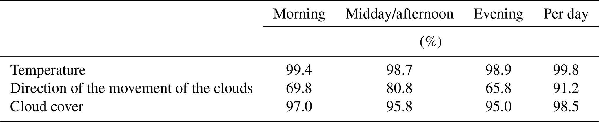

Figure 1Example of Morin's notes (source: Institute of History/Oeschger Centre for Climate Change Research, University of Bern). Column 1 shows the day of the month; column 2 shows the day of the lunar cycle; column 3 shows the conjunction, opposition, and other aspects of the moon and the sun; column 4 shows the conjunction, opposition, and other aspects of the planets; column 5 shows the thermometer measurements; column 6 shows the hygrometer measurements; column 7 shows the barometer measurements; column 8 shows the wind direction; column 9 shows the wind strength; column 10 shows the direction of the movement of the clouds; column 11 shows the regional origin of air; column 12 shows the speed of the clouds; column 13 shows the cloud cover; column 14 shows intensity and duration of rainfall; column 15 shows fog, snow, small hailstones, thunder perihelion, and the color of the sky; column 16 gives miscellaneous observations, such as earthquakes, comets, and halos. For more details, see the text.
2.1.2 Time of the observations
Most of the time, Morin made three observations per day, but there are at least some days on which he measured four, five, or six times. The specific measurement times are uncertain, but due to his ascetic life it is suggested that he did the first measurement around 06:00 UTC+1, the second measurement between 11:00 and 14:00 UTC+1, and the third measurement between 18:00 and 19:00 UTC+1 (Pfister and Bareiss, 1994). Cornes et al. (2012) estimated the observation times: 06:00, 15:00, and 19:00 UTC+1.
2.1.3 Location of the observations
The location of the so-called big thermometer changed several times, which is known from the rare notes of Louis Morin (Legrand and Le Goff, 1987). Until October 1685, he lived on Quinquempoix Street (number 1 in Fig. 2), then until June 1688 in the Hotel Rohan-Soubisse (number 2 in Fig. 2), where the National Archives are located today. Until his death in 1715, he lived in the abbey Saint-Victor (number 3 in Fig. 2), which is located at the city border next to the Seine (Legrand and Le Goff, 1987; Pfister and Bareiss, 1994).
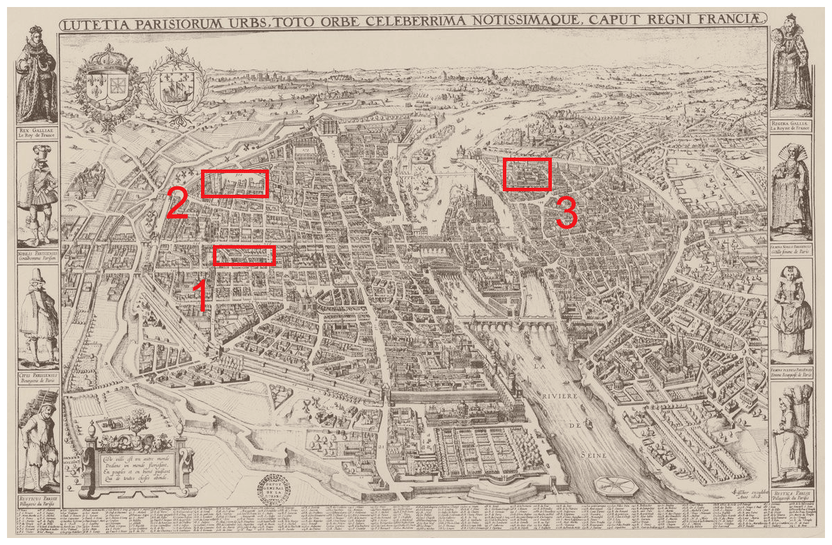
Figure 2A map of Paris (Visscher, 1618). The marked locations show where Morin lived. Until October 1685, he lived on Quinquempoix Street (1), then until June 1688 in the Hotel Rohan-Soubisse (2), where the National Archives are located today, and until his death in 1715 he lived in the abbey Saint-Victor (3), which is located at the city border next to the Seine (source: https://gallica.bnf.fr/, last access: 4 January 2022/Bibliothèque nationale de France).
2.2 Reference data
We adopted quality-assured hourly and monthly data from ERA5 (1979–present) to compare the direction of the movements of the clouds and the cloudiness to contemporary conditions (Hersbach et al., 2018a, 2019). We chose a reference period of 30 years as suggested by the WMO (2003) from 1981 to 2010. Furthermore, we used hourly ERA5 data on temperature and precipitation to statistically analyze the measurement times of Morin and to validate the thermometer (Hersbach et al., 2018b). As a reference period for the temperature data, we used the observations of E-OBS version 21.0e (Cornes et al., 2018) for the common period from 1961 to 1990. Furthermore, we included in our study the grape harvest dates (GHDs) from Beaune (Labbé et al., 2019), the Central England Temperature (CET, Manley, 1974), and winter temperatures from De Bilt (Van Den Dool et al., 1978).
3.1 Digitalization process
Although we did get digitized data from Christian Rohr and Christian Pfister, given that they had already been processed and did not cover the entire time span of the copies, we digitalized the notes for the years 1665 to 1713. Thus, we digitalized about 140 000 values and checked the digitized data for implausible values and typos. For temperature data, we further consulted already digitized data from Bern to check for mistakes.
3.2 Missing data
We kept the original data and did not correct the missing values, except when performing the impact analysis for the temperature. In detail, smaller gaps with one or two consecutive missing values were filled by the mean of the day before and the day after the missing value. Thus, we filled up 60 values for the morning temperature, 131 values for the midday/afternoon temperature, and 114 values for the evening temperature.
3.3 Calibration and homogenization of the thermometer
We know that the Florentine thermometer was already known in France (Paris) because it is documented that Ismaël Boulliaud got one in 1658 (Legrand and Le Goff, 1987; Rousseau, 2013; Camuffo et al., 2020). The conventional graduation of the Florentine thermometer is different to the one used by Morin. It is supposed that he used three different thermometers because the graduations of the temperature measurements differ when viewed over time. The first was used from 1 February 1665 to 12 April 1670 with nine divisions. The second was used from 13 April 1670 to 31 August 1675 with 11 divisions. The third (big thermometer) was used from 1 October 1675 to 13 July 1713 with 15 divisions. Furthermore, each of these divisions is separated into 10 parts (see Legrand and Le Goff, 1987, Fig. 2). It is supposed that Morin used the following calibration: put the thermometer in ice, into which salt was added. After an appropriate time, while keeping the thermometer in the ice, mark the position of the spirit. Then put the thermometer into a cellar, which is cut off from the outside world. Measure the temperature again and make a mark. Split the space into 15 divisions and label the marks with numbers using the mark in the cellar as a point of origin (Legrand and Le Goff, 1987; Rousseau, 2009). Due to the low resolution of the thermometers used before 1675, we only used the big thermometer for further calculations. Using proxy data, Legrand and Le Goff (1987) have identified two time periods which are characterized by identical climatic conditions. These two periods cover the measurements of Morin from 1676 to 1713 and the measurements of the Observatory of Paris from 1816 to 1852. So, Legrand and Le Goff (1987) calculated a linear relationship between the maximum temperatures, the minimum temperatures, and the measured temperature (TM) of the two time periods and used three different linear regression formulas for the maximum temperatures (Eq. 1), for general minimum temperatures (Eq. 2), and for significant cold minimum temperatures (Eq. 3):
To calculate the minimum temperature in Eq. (1), TM represents the smallest measured value per day. In addition, to calculate the maximum temperature in Eqs. (2) and (3), TM represents the highest measured value per day. The entry of TM consists of a letter (f, froid – cold; c, chaud – warm) and a number (see Fig. 1). For entries which are noted with c, TM is multiplied by the following value, and for entries which are noted with f, TM is multiplied by the negative value of the following value. We used this calibration to receive values in degrees Celsius. Furthermore, Rousseau (2009) suggested that the years from 1676 to 1680 should be corrected because GHDs in that period differed significantly from the temperature measurements of Morin. So, Rousseau (2009) compared the monthly means of the Morin measurements with the CET and modified the months between 1676 and 1680 with the values (January to December) , because he found significant differences compared to the CET (Manley, 1974) and GHDs. However, we did not apply this proposed change because the magnitude of the change seems to us to be too large. Furthermore, because this change refers to the monthly mean, it is difficult to make an exact attribution to the minimum and maximum temperature. The extension to months outside the growing season is also debatable. Another point is that there is no documented change in Morin's circumstances in terms of location change and so on in this period. Additionally, a comparison with De Bilt winter temperatures shows no significant differences. However, it has to be mentioned that we do agree that the temperatures are unusually high for these years noted by Morin (see Table 2).
Based on our analyses, we found an inhomogeneity of the temperature measurements. This inhomogeneity concerns the years 1688–1691 and is characterized by a diurnal temperature range (DTR) that is too small. Nevertheless, the comparison of Tmean with proxy data and the CET does not reveal a significant bias. Therefore, we need a correction that keeps Tmean constant and corrects Tmin and Tmax in equal parts. To correct this inhomogeneity, we propose the following correction: the values refer to the months January to December and are to be added to Tmax and subtracted from Tmin (see Sect. 4.1.1 for more details). Nonetheless, we will use the original data for our analyses but provide a homogenized time series in the supplementary dataset. This homogenized time series takes into account the correction by Rousseau (2009) and the inhomogeneity we detected.
4.1 Temperature
Based on the daily available temperature data, we perform an impact analysis. However, to check the reliability of the values, it is necessary to perform a statistical analysis beforehand and to compare with proxy data.
4.1.1 Qualitative and quantitative cross-validation
As previously mentioned, the measurement times, the measuring device used, the liquid used, and the location of the measuring device are not explicitly noted by Morin and are therefore based on assumptions. Consequently, it is necessary to validate Morin's measurement data with alternative methods to refer to metadata. Although cross-validations with other measurement series are possible, only the CET measurement series exists at the same time. This series can only be used as a limited comparison because the climate in Great Britain differs from that on the mainland. This leaves only statistical possibilities and the use of proxy data.
Due to the fact that the measurement times can only be determined based on Morin's ascetic lifestyle, we looked for a way to validate these measurement times. Given that the average of the diurnal variation of the temperature follows a unimodal distribution, we performed a statistical approach by calculating the number of days on which the temperature, which usually indicates a lower temperature value, exceeds the usually higher temperature (e.g., Tmi<Tev). After that, we compared the results with the ERA5 data for the reference period from 1981–2010. In detail, we calculated the time index (TI) after the following formula:
Thereby, the measurements by Morin are indicated as morning temperature (Tmo), midday temperature (Tmi), and evening temperature (Tev). Because earlier papers are based on suggestions regarding when the measurements of Morin were done most properly, we integrated the ERA5 data with the variables Ti, Tj, and Tk, where , , and . So, means, for example, the number of days when the mean temperature of 17:00 and 18:00 UTC+1 exceeds the mean temperature of 14:00 and 15:00 UTC+1. We calculated the TI multiple times for reasonable time triples (e.g., ) and looked for the minimum of TI, which can be seen as the sum of the linear anomaly of each measurement. This method can only be used as an indicator because there are many underlying premises that have to be assumed. Nonetheless, we think that by taking a longer time period, this method can be seen as an additional indicator for making a statement about Morin's measurement times. Four triples showed a TI<19.00: TI=11.50 for the triple, TI=17.50 for the triple, TI=18.58 for the triple, and TI=18.77 for the triple. This supports the hypothesis of the measurement times from Cornes et al. (2012) and contradicts the assumption of the measurement times at midday/afternoon (11:00 to 14:00 UTC+1) from Pfister and Bareiss (1994). Additionally, it is a practical advantage for the analysis of temperature extremes because Morin performed a measurement near the daily minimum and maximum temperature. Nevertheless, taking a closer look at the annual distribution of the number of days when Tev>Tmi, it can be seen that there is a strong variation, whereas there is a nearly uniform distribution on a monthly basis (see Fig. A1).
Morin also documented snow days and rainy days. This allows us to determine the temperature at which snowfall occurs and vice versa. It is generally assumed that snowflakes begin to melt at a temperature of 0 ∘C. However, this is not true in detail because there are spatial differences; the melting point is dependent on pressure and even more on humidity. Increasing pressure leads to an increasing melting point temperature, and increasing humidity also leads to an increasing melting point temperature. It is found that the phase transition occurs over a fairly wide temperature range from about −2 to +4 ∘C over (low-elevation) land and from −3 to +6 ∘C over ocean (Dai, 2008). Jennings et al. (2018) found that the air temperature at which rain and snow fall in equal frequency varies significantly across the Northern Hemisphere, averaging 1.0 ∘C and ranging from −0.4 to 2.4 ∘C for the 95 % confidence interval. The results of Jennings et al. (2018) showed that the threshold temperature is about 1.5 ∘C in Paris. This means that an investigation of the melting point temperature or snowfall frequency can provide information about whether it is an indoor or outdoor measurement and/or if the lower calibration point is accurate. The case in which deviations cancel themselves is unlikely. So, if the temperature of the 50 % snowfall frequency threshold, calculated from Morin's measurements, is somewhat equal to 1.5 ∘C, then we assume that he performed an outdoor measurement and that the lower calibration point is accurate.
The results are shown in Fig. 3; the solid black line shows the snowfall frequency as a function of the temperature for all measurements. The green, orange, and blue lines represent the results for the measurements in the morning, at midday/afternoon, and in the evening, respectively. The threshold temperature at 50 % of the ERA5 dataset equals 0.8 and 1.5 ∘C for the Morin dataset. Even though the threshold temperature of the snowfall frequency at 50 % fits well, the slope of the function is smaller than expected. The differences between the times of measurement are interesting. The morning temperature of the 50 % snowfall frequency is just slightly underestimated, while the evening and midday/afternoon temperatures of the 50 % snowfall frequency show moderate and strong positive deviations, respectively.
Two problems in the methodology arise: (1) rain or snow was measured by Morin by eye; i.e., if Morin noted snow, then it may have fallen in a certain time period, while temperature was read at fixed times. (2) The table of Morin's measurements illustrates another problem: Morin used six possible entry points for precipitation at the respective measuring points for the temperature and in between. Some entries are made on the line, which separates 2 d. Considering Morin's strict daily routine, we interpret these measurements as taken at 02:00 UTC+1, when Morin used to get up. The next value was noted in the line with the first temperature measurement. So problems (1) and (2) affect the temperature measurement in the morning only slightly because the temperature difference between 02:00 and 07:00 UTC+1 changes only slightly in winter. However, for the midday/afternoon and evening temperature these points are more problematic. In the case of the midday/afternoon temperature, it may have occurred that it snowed at lower temperatures (e.g., at 10:00 UTC+1), while the temperature was measured at the time of the daily maximum. In the case of the evening temperature, an attribution is difficult. Here, it seems to us that points (1) and (2) do not matter as much as the effect of the calibration. The calibration has been developed for the maximum temperature and thus, when applied to the evening temperature, will result in higher temperatures at the 50 % snow–rain threshold.
So, the morning measurement is the least affected by the methodological shortcomings, and this is also seen in Fig. 3. The majority of values in the morning lead to an acceptable result averaged over all measurements. Deviations of midday/afternoon and evening measurements can only be explained qualitatively and not quantitatively and are therefore not trustworthy. Nevertheless, we conclude that this method, due to the good agreement of the morning measurement with the ERA5 data, shows that Morin's thermometer is trustworthy in the 0 ∘C range and that he performed an outdoor measurement.

Figure 3Snowfall frequency curves calculated using Morin's observations of the morning (green), midday/afternoon (orange), and evening (blue). The black line includes all of Morin's measurements, and the red line shows the mean of the ERA5 hourly data.
Camuffo and della Valle (2016) and Camuffo et al. (2017) suggested an index to recognize indoor or outdoor exposures and room ventilation. This is a useful index because it can point out the buffering capacity of the building structure on an hourly timescale, which is named the normalized diurnal range (NDR) (i.e., the ratio between the observed diurnal temperature range, or a given portion of it, and the same but measured outdoors in the 1961–1990 reference period). The diurnal range has a marked seasonal character. Normalization is applied to remove the seasonal dependence and to point out how much the observations are damped in comparison with the outdoor cycle. NDR can be considered to be a room fingerprint, which is strictly linked to the room ventilation, solar exposure, and use. In this paper, NDR has been calculated with the formula
where Tn,6 and Tn,15 are the readings of the nth calendar day at 06:00 and 15:00 UTC+1, Tn,6 is close to the daily minimum and Tn,15 to the daily maximum, the difference equals the diurnal range of the nth calendar day, nSP is the total number of days of the selected period (SP), and the label RP refers to the 1961–1990 reference period (E-OBS). NDR =0 when the buffering capacity is very large and the ventilation is poor, and NDR =1 when the thermometer is kept outside, well ventilated, and far from walls such as modern weather stations. The formula calculated with our datasets leads to a value of 0.90. So we assume that the temperature measurement was performed outside and it was well ventilated with small influences from walls and so on. However, if one divides the periods into the three different localities where Morin lived, then differences arise for this parameter. We calculate NDR =0.80 from 1675 to October 1685, NDR =0.80 from November 1685 to June 1688, and NDR =0.95 from July 1688 to 1713. In analog to that, these differences can be seen when calculating the diurnal temperature range (DTR; see Fig. A2). In Fig. A2b, significantly low DTR values can be detected in the years 1689–1691. Thus, we analyzed these years in more detail and normalized Tmin and Tmax in Fig. A3a by monthly mean values calculated using Morin's measurements from 1676–1713. Usually, the normalized values should at least largely overlap. However, it is evident in Fig. A3a that there is a discrepancy, especially in the warmer months. Whether this discrepancy results from Tmin or Tmax can be determined by comparing Tmean with both proxy data (GHDs) and CET. But these comparisons show no discrepancies in these years. Consequently, as already seen in Sect. 3.3, we conclude that Tmean is quantitatively correct and thus Tmin and Tmax can be corrected in equal parts as follows in the years 1689–1691: . These values represent the months January–December and indicate half the difference between the normalized Tmin and Tmax. Thus, these values are to be subtracted from Tmin and added to Tmax to homogenize these years (Fig. A3b). This time period is directly after Morin's second change of residence (June 1688). It is possible that he could not read the thermometer at the times of the daily maxima and minima due to the change of residence for a few years. This hypothesis would be supported by Fig. A1a because an unusually high number of days when Tev>Tmi was noted in those years.
Another possibility to validate the temperature data is to compare them with proxy data, such as with grape harvest dates (GHDs). Due to the high control of temperature on grape ripening, GHDs are linked to the growing season temperature (GST: mean, e.g., Chuine et al., 2004; Meier et al., 2007; Labbé et al., 2019, or maximum temperature, e.g., Daux et al., 2012, averaged over April to July, e.g., Labbé et al., 2019, April to August, e.g., Chuine et al., 2004; Meier et al., 2007, or April to September, e.g., Daux et al., 2012). Several authors have evidenced a statistically significant correlation between GST and GHDs. For example, Daux et al. (2012) showed that high correlations are obtained between GHD regional composite series and the temperature series of the nearest weather stations. Moreover, the GHD regional composite series and temperature correlation maps show spatial patterns similar to temperature correlation maps (Daux et al., 2012). Furthermore, others have quantified the change in GHDs in terms of the variation of the temperature. Menzel (2005) stated that the variation of the GHDs of a mean European series was 10.0±0.9 d for 1 ∘C variation of the GST. Meier et al. (2007) showed that 12 d of grape harvest difference correspond to around 1 ∘C April to August temperature for varieties grown in Switzerland. Chuine et al. (2004) calculated a linear correlation coefficient between reconstructed temperatures and GHDs of 0.75±0.07 for Paris. However, Labbé et al. (2019) constructed GST in a different way with a statistical model, which led to a rate of 10 d per 0.61 ∘C. The difference of his calculations is that he weighted the months differently and used the months from April to July.
In Fig. 4, we have plotted the mean temperature of the months April to August for comparison to the GHDs. The calculated correlation between GHDs and Tm is −0.75 (−0.50 for Tmax). Compared to the present time, the GHD of the LMM was slightly earlier than in the reference period from 1961–1990. Surprisingly, the mean temperature of the months April to August is higher in the LMM than the mean temperature of the reference period from 1961–1990. So, we obtain over the time periods (GHD). This means that the temperature difference should be more or less 0 between these time periods, which is fulfilled for the mean of the maximum temperature: (GST). A slightly higher difference occurs when looking at the mean temperature: (GST).
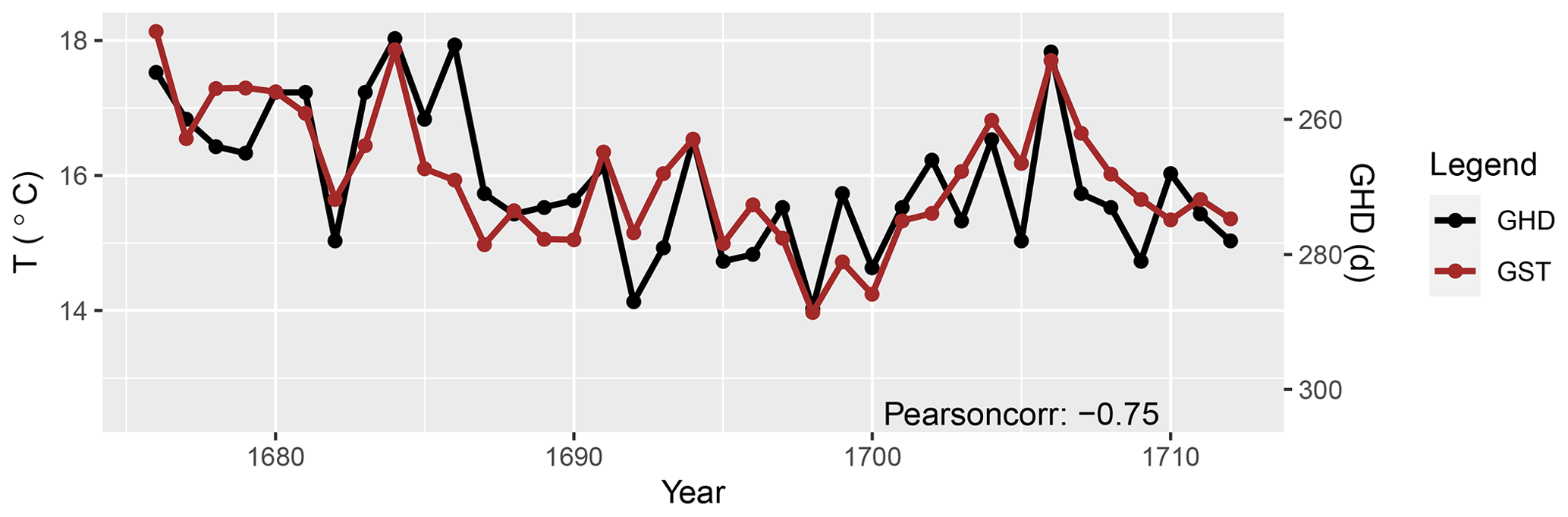
Figure 4Comparison between GST of Tm in Paris and the grape harvest dates (GHDs) from Beaune (Labbé et al., 2019) in the LMM. The Pearson correlation index equals a value of −0.76.
We examined Morin's measurements for inhomogeneities with respect to a non-northward orientation of the thermometer (Böhm et al., 2010) and inhomogeneities caused by the use of alcohol thermometers (Camuffo and della Valle, 2016). No abnormalities seem to occur on either point.
4.1.2 Seasonal temperature anomalies
The LMM is generally considered to be the second coldest period in the LIA, after the Spörer Minimum. Although it is a short period, the characteristics are different and interdecadal variability is high. Figure 5 shows the seasonal temperature anomalies of each meteorological season in reference to the mean value of 1961–1990. The anomalies show that the general statement that the LMM was a cold period can be discussed; that is, warmer months (MAM, JJA) reflect small anomalies and colder months (SON, DJF) show negative deviations with respect to the reference period. A strong variability can be observed in the DJF season, which causes extremes for Tmin and Tmax between 1675 and 1690, almost year after year. The decade from 1691 to 1700 is known as the coldest period in the LMM, which is confirmed in Fig. 5 for each season to be stronger for Tmax (−1.9 ∘C anomaly in DJF) and somewhat weaker for Tmin (−1.8 ∘C anomaly in DJF). The decade from 1701 to 1710 experiences warming across all seasons that is strongly pronounced in JJA and DJF and somewhat weaker in MAM and SON. An interesting aspect is that Tmax between 1691 and 1700 shows several years with positive anomalies for MAM and JJA. This also can be seen in the GHDs, which do not reflect the cold period in the LMM. In summary, the decades 1691–1700 and 1701–1710 stand in contrast: the former as a pronounced cold period and the latter as a warm period. Table 2 shows the anomalies of Tmin, Tmax, and separated into decades and seasons. Extraordinary positive anomalies appear between 1675 and 1680 for MAM and JJA (see Sect. 3.3), and extraordinary negative anomalies appear as expected in DJF and SON in the last 2 decades of the 17th century. With respect to the mean temperature three DJF seasons fall below an anomaly of −4 ∘C, namely the winters of 1683/84, 1694/95, and 1696/97. Interestingly, the notorious winter of 1708/09 is not particularly pronounced in terms of mean temperature because December 1708 was moderate and devastatingly cold temperatures (Tmin up to −18 ∘C) were restricted to January.
Table 2Anomalies of Tmin, Tmax, and Tmean divided into seasons (DJF, MAM, JJA, and SON) with respect to the reference period (E-OBS: 1961–1990). The CET is given as a comparison in the brackets of the mean temperatures.
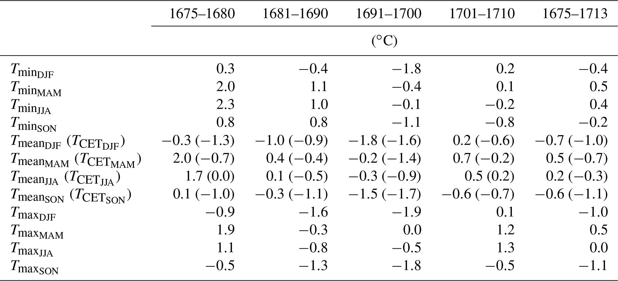
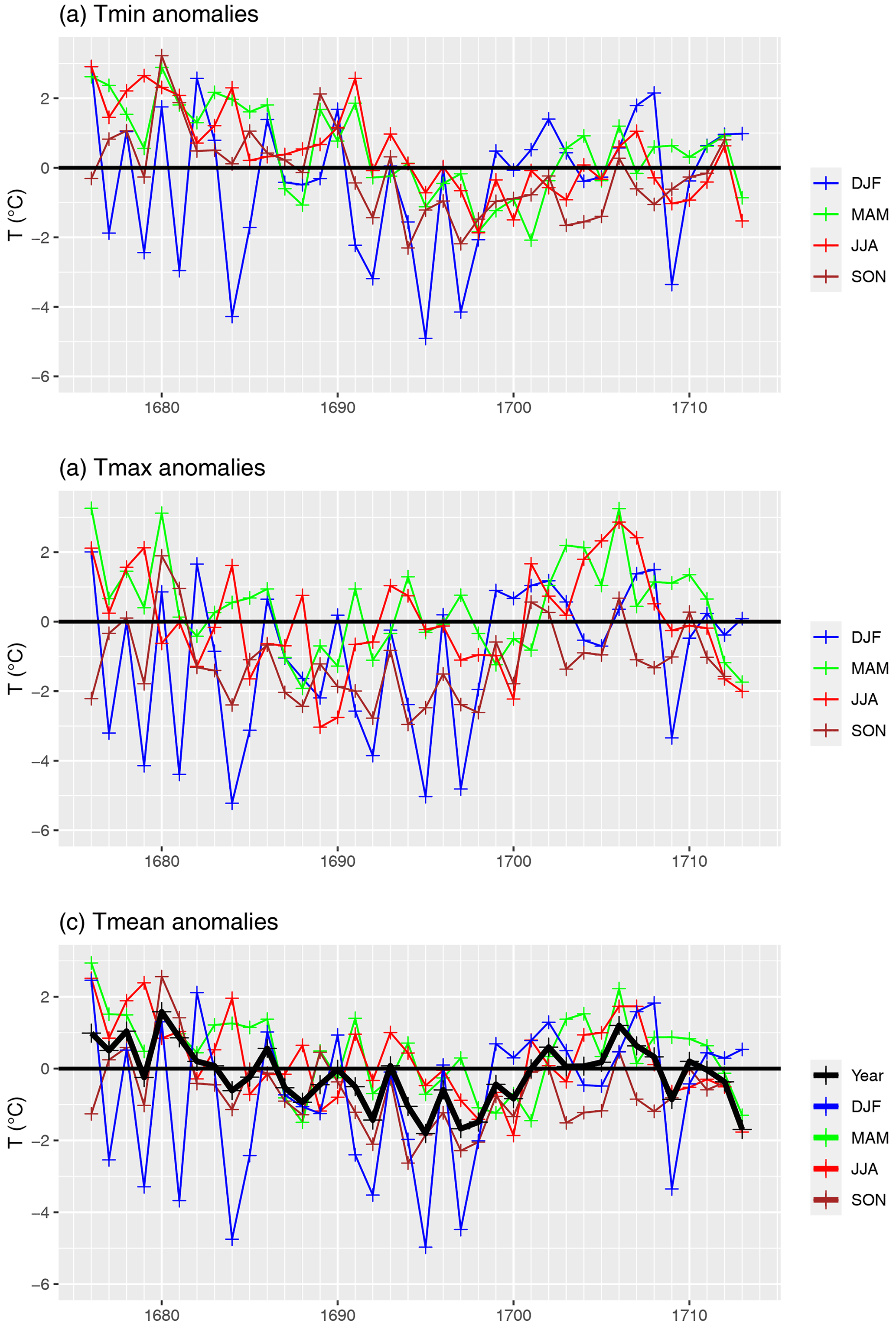
Figure 5Seasonal temperature anomalies (DJF: December, January, February; MAM: March, April, May; JJA: June, July, August; SON: September, October, November) for (a) minimum, (b) maximum, and (c) mean temperature from 1676–1713 with respect to the mean value from 1961–1990 (E-OBS). In addition, in (c) the annual mean temperature is shown.
4.1.3 Impact analysis
To be able to examine the different characteristics of this period in more detail, we have carried out an impact analysis. An impact analysis shows a more detailed picture of the circumstances or the influence of the weather and/or climate on humans. Consecutive warm and cold days dramatically complicate living conditions and lead to lower crop yields, famine, and so on. For the cold season (DJF), the indices FD0 (number of days on which the temperature falls below 0 ∘C) and ID0 (number of days on which the temperature stays below 0 ∘C) were calculated. The results (see Fig. 6) reveal a high variation of cold winters, which occur more frequently in the decade 1691–1700. However, some devastating winters with a high number of ice days (ID0 20–30) are found in the last decade of the 17th century, namely 1676/77, 1678/79, 1680/81, 1684/85, and 1708/09. Only the winters 1694/95 and 1696/97 are found in the cold decade. However, when measured by the number of frost days, the last decade of the 17th century remains the coldest period.
For the warm season (JJA), the indices SU25 (days with a maximum temperature value above 25 ∘C for summer days) and SU30 (days with a temperature value above 30 ∘C for heat days) were examined. Up to the year 1690, there is a strong variability with alternating higher and lower values for SU25, as well as a gradually disappearing SU30 value. This follows a decade with moderate summers in the decade 1691–1700 (i.e., moderate SU25 values and SU30 values towards zero). The warmer first decade of the 18th century is also evident here with high SU25 values (>40 d for the summers of 1701, 1704, 1705, 1706, and 1707) and also with an increase in SU30 values in the same years. This again confirms that the summer months in the LMM can be described as moderate.
Table 3Anomalies of FD0, ID0, cons. cold days, and cons. ice days for the season DJF and SU25, SU30, warm waves, and heatwaves for the season JJA with respect to the reference period (E-OBS: 1961–1990).
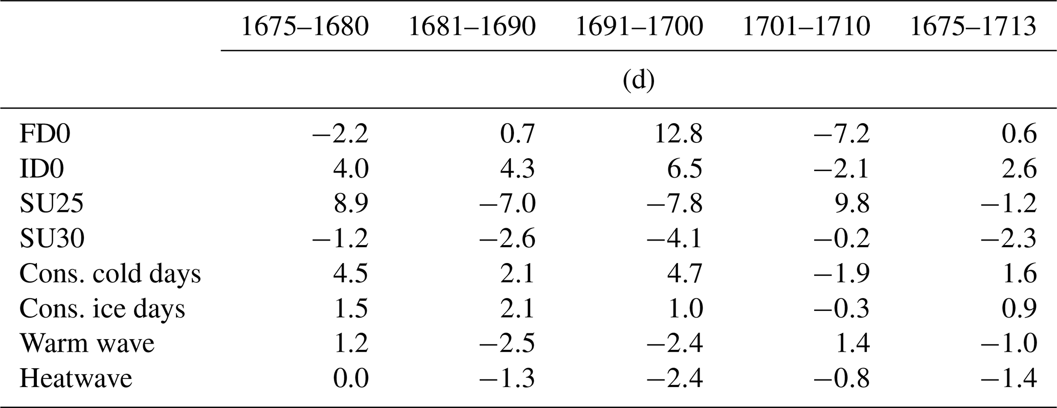
An even more differentiated picture emerges when looking at the consecutive cold days,or ice days (Fig. 7). Winter 1676/77 (42 consecutive cold days) clearly stands out. On average, the last period of the 17th century is again the most striking, but compared to the winter 1676/77 these appear moderate with respect to consecutive cold days. The winter of 1708/09, which is known as a devastating winter, has the most ice days. This winter is characterized by a mild December, a freezing cold January with temperatures down to −18 ∘C, and a cold February. This is why the winter of 1708/09 is not outstanding with respect to the mean of Tmin, Tmax, and FD0. The most consecutive warm days and heat days are again to be found in the first decade of the 18th century. In summary, the picture is more differentiated; exceptional weather conditions cannot be limited to the supposedly cold period of the last decade of the 17th century and the supposedly warm period of the first decade of the 18th century.

Figure 6(a) Calculation of the indices FD0 (number of days on which the temperature falls below 0 ∘C) and ID0 (number of days on which the temperature stays below 0 ∘C) for the cold season (DJF). The horizontal lines indicate the respective average values over the entire period (: sky blue; : blue; : upper black line; : lower black line). Meanwhile, panel (b) shows the calculation of the indices SU25 (days with a temperature value above 25 ∘C) and SU30 (days with a temperature value above 30 ∘C) for the warm season (JJA). The horizontal lines indicate the respective average values over the entire period (: red; : dark red; : upper black line; : lower black line).
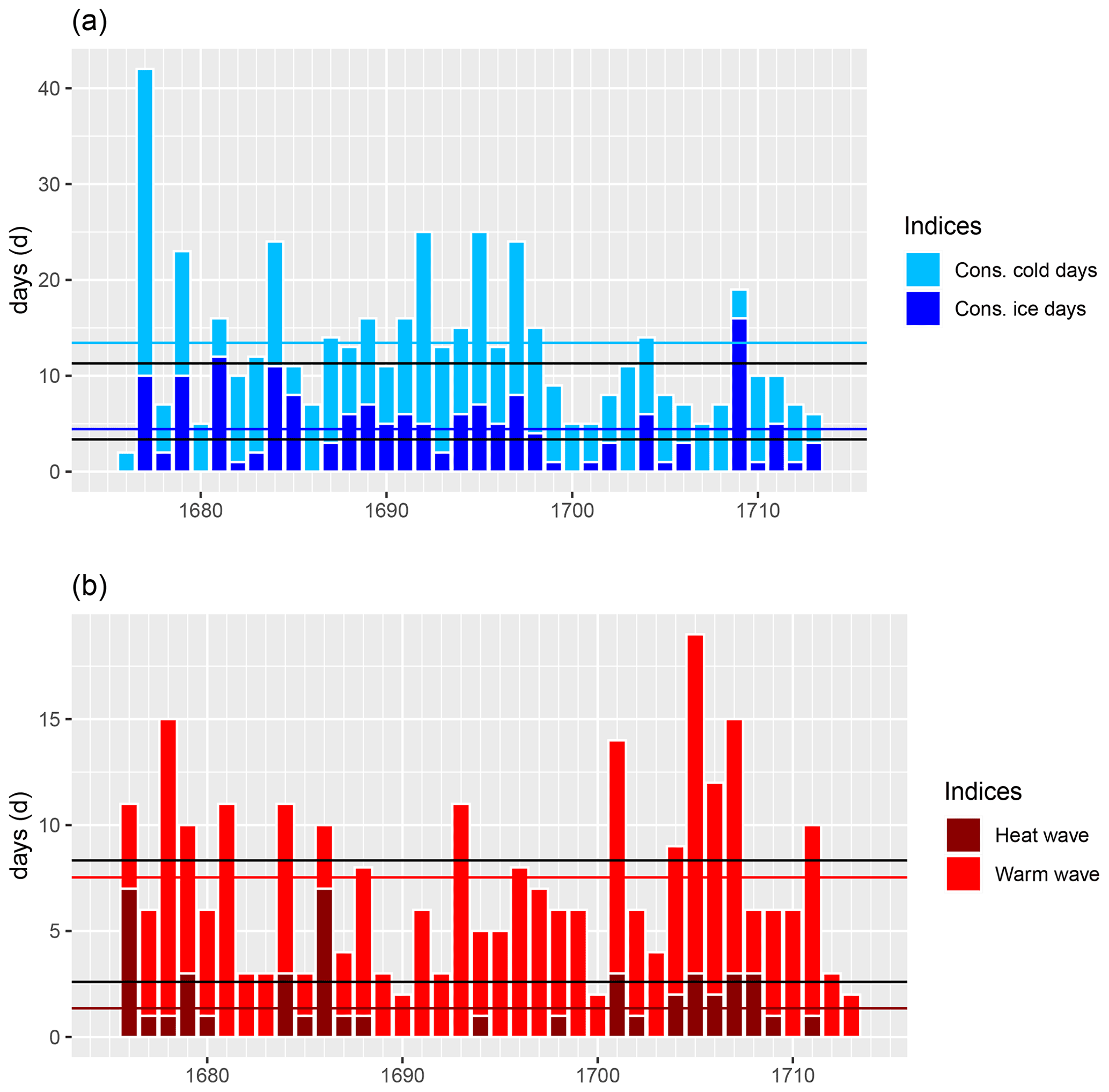
Figure 7Calculation of (a) maximum number of consecutive cold days and maximum number of consecutive ice days for the cold season (DJF). The horizontal sky blue line indicates the mean of consecutive cold days and the blue line the mean of consecutive ice days. The horizontal upper (lower) black line indicates the mean of consecutive cold (ice) days of the reference period. Meanwhile, panel (b) shows warm waves (consecutive days of ∘C) and heatwaves (consecutive days of ∘C) for the summer season (JJA). The horizontal red line indicates the mean of warm waves and the dark red line the mean of heatwaves. The horizontal upper (lower) black line indicates the mean of warm waves (heatwaves) of the reference period.
4.2 Cloud cover
The scale of Morin's readings reaches from 0 to 4, on which 0 means sky completely free and 4 means sky completely cloudy (analog to his notes on fog). The readings can be assumed to represent the total cloud cover (TCC). TCC series were frequently given in oktas (WMO, 2021); fine: 0 (sky clear) to 2 (2/8 of sky covered) oktas; partly cloudy: 3 to 5 oktas; cloudy: 6 to 7 oktas; overcast: 8 oktas (sky completely covered); sky obstructed from view: 9 oktas (e.g., fog). To obtain comparable quantities, Morin's original data are multiplied by a factor of 2. Because Morin also recorded foggy days, we weighted records that had values of 3 and 4 by 9 oktas. This allows a quantitative comparison to present TCC series. In Fig. 8 the TCC series is plotted from 1665–1713. In Fig. 8a the black line indicates the yearly mean of the TCC and the colored lines represent the mean TCC of DJF, MAM, JJA, and SON. A remarkably high TCC appeared in the years 1692 and 1693, whereas the highest seasonal value appeared in the year 1668. Remarkably low values appeared in fall 1669 and in winter 1691. A positive linear trend in TCC between 1670 and the early 1690s is noticeable. The reason for that can be seen in Fig. 8b and may be due to a differing estimation of the cloud cover. The highest value (4) increases, while the second highest value (3) decreases between 1670 and the early 1690s.
Clouds contribute to both cooling and warming the Earth’s surface due to their high albedo and capacity to absorb infrared radiation (Mace et al., 2006; Zelinka and Hartmann, 2010). Consequently, a statement about a correlation of temperature and cloud cover is difficult. Furthermore, traditional observations lack objectivity: for example, regarding the estimation of TCC and the determination of cloud types (Sanchez-Lorenzo et al., 2012). In this context, changes in observing practices, time of observations, and different observers can introduce biases that affect the homogeneity of the series (Sanchez-Lorenzo et al., 2012). For these reasons, a quantitative comparison between Morin's TCC series and the present TCC series is problematic. However, several publications present the relationships between the observed worldwide long-term decrease in daily temperature range (DTR) and the systematic increase in cloud cover (Dai et al., 1999; Sun et al., 2000; Cox et al., 2020), and trends can be found in different seasons and different decades. In Table 4 the percentage change in Morin's TCC series is shown per decade, with the mean of the ERA5 data from 1981 to 2010 as a reference. The seasonally mean TCC from 1665–1713 shows a significantly lower value for all seasons. The highest anomalies are observed in 1665–1680, when for instance the spring season has a 27.0 % (1665–1670) and a 30.4 % (1671–1680) lower value with respect to the mean of the ERA5 data (1981–2010). Over the entire series from 1665–1713 high seasonal anomalies, with respect to the mean of present TCC series, are obtained in MAM (−20.9 %), JJA (−18.4 %), and SON (−18.0 %), while a smaller anomaly can be seen in DJF (−14.0 %).
Table 4Anomalies in Morin's TCC notes with respect to the mean of present time series TCC (ERA5 Dataset; 1981–2010).
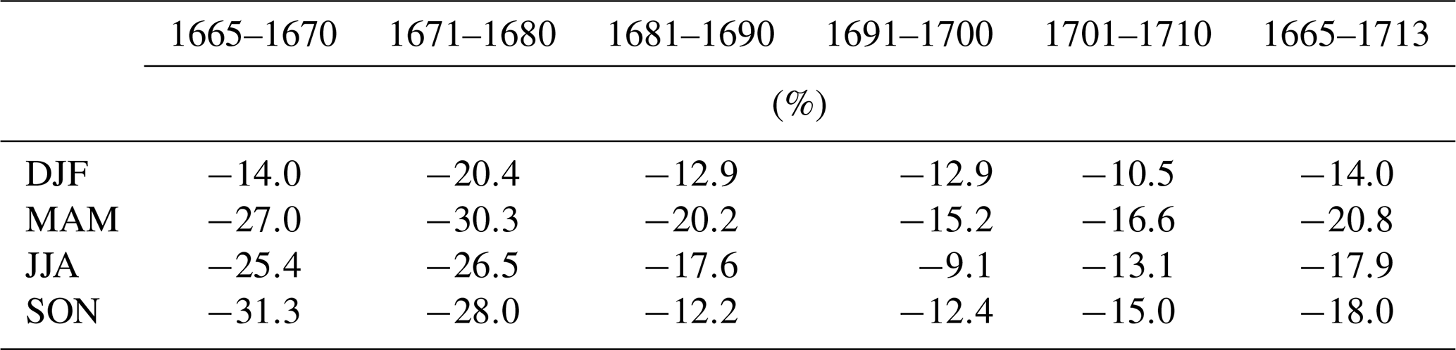
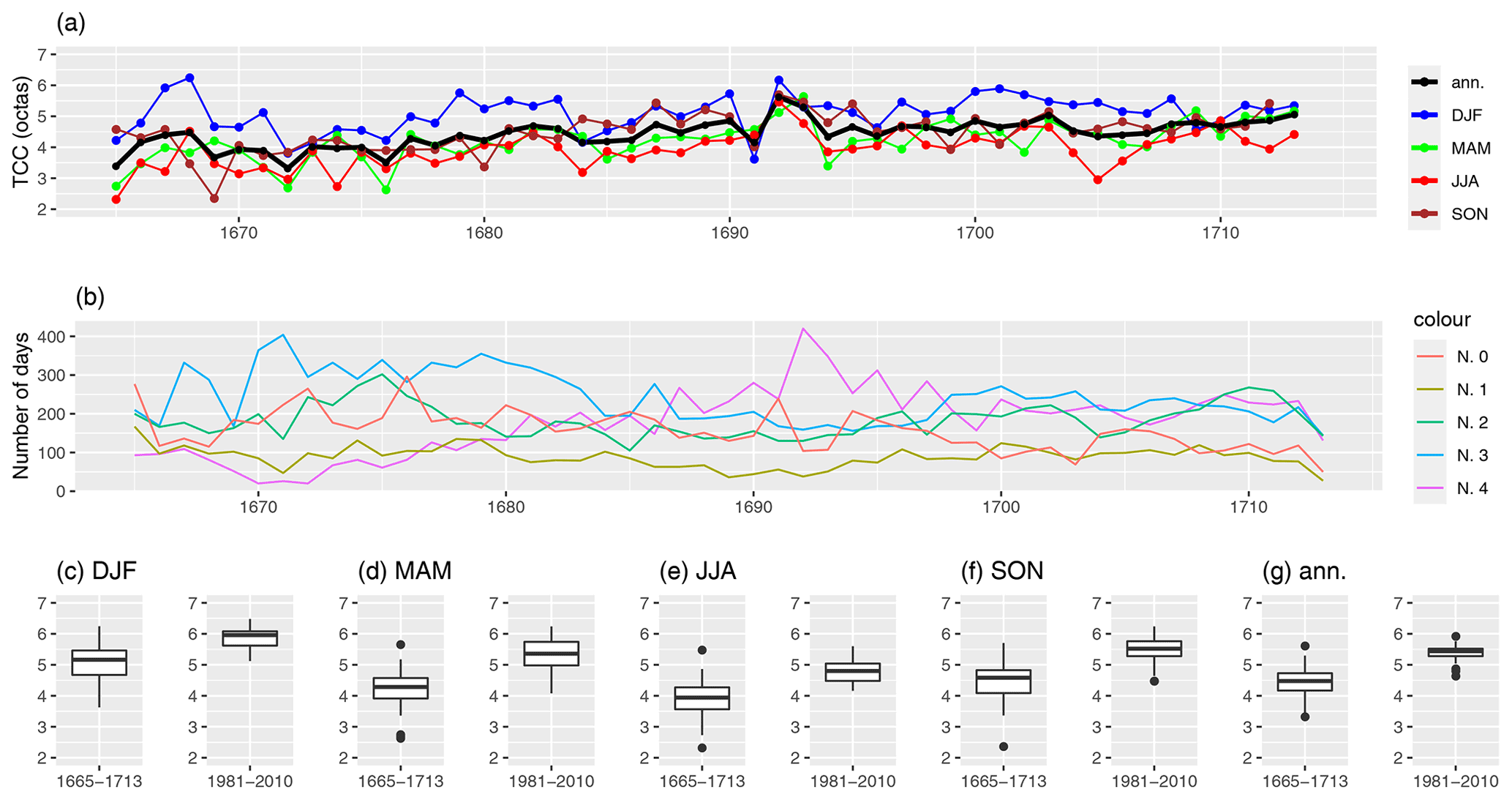
Figure 8Total cloud cover (TCC) in oktas from Louis Morin's readings is shown in panel (a): yearly means of DJF, MAM, JJA, SON, and the whole year. In panel (b) the different notes (0 to 4) are shown on a timeline. The box plots show the seasonal and annual means of the time period of Morin's measurements and the mean of the data from ERA5 for 1981–2010 (c–g).
4.3 Direction of the movement of the clouds
To assess the atmospheric circulation during the LMM, we calculated the mean of Morin's sub-daily notes by vector addition. We then analyzed the data using the approach of Mellado-Cano et al. (2018). Accordingly, we computed four directional indices (DIs), one for each cardinal direction: northerly (NI) , easterly (EI) , southerly (SI) , and westerly (WI) . They are defined as the percentage of nonmissing days per month with cloud motion from that direction (Wheeler et al., 2010; Mellado-Cano et al., 2018).

Figure 9Seasonal time series of the directional indices (DI: NI, EI, SI, WI) in percentage of nonmissing days from 1665 to 1713. The individual points indicate the mean per season of the direction of the movement of the clouds.
To illustrate the raw data, Fig. 9 shows the seasonal time series of the DIs from 1665 to 1713. The reduced number of just four indices allows us to easily interpret the main characteristics of the synoptic-scale circulation and the associated impacts in terms of temperature and precipitation. Thus, for example, an increased persistence of EI indicates dry advection from land, and the NI is related to cold advection from higher latitudes. An increased persistence of WI indicates wet advection from the ocean, and the SI is related to warm advection from lower latitudes. Furthermore, an increased persistence of WI in the DJF season indicates warm advection from the ocean, whereas an increased persistence of WI in the JJA season indicates cold advection from the ocean. Apart from a high variability, a rise in the WI over the time period can be noted in each season. This confirms earlier studies, which are based on ship logbooks (Wheeler and Suarez-Dominguez, 2006; Mellado-Cano et al., 2018). The DJF season indicates that the colder decade (1691–1700; see Sect. 4.1) is marked by a strong EI and a weaker WI. In contrast, the decade from 1701–1710 is characterized by a dominating WI in the DJF season. This means that the synoptic-scale circulation caused the unusual cold conditions of the DJF season in the 1691–1700 decade. However, a stronger assertion of which driving factors caused the change in the circulation cannot be made based solely on Morin's measurements. The years from 1699 onwards are indicated by an unusually high percentage of WI, which seems to correlate with the warming. Lockwood et al. (2017) find that several factors are responsible for explaining the cold conditions between 1570 and 1726. Thus, the cold could be explained not only by the reduced number of sunspots or possible volcanic activity but also by possible other factors. Moreno-Chamarro et al. (2017) demonstrate that such exceptional wintertime conditions arose from sea ice expansion and reduced ocean heat losses in the Nordic and Barents seas, driven by a multicentennial reduction in the northward heat transport by the subpolar gyre. This would lead to blocking situations in winters, which would reduce the airflow from the western direction. This explanation is consistent with our results of the directions of the movement of the clouds.
Figure 10 shows the seasonal DIs averaged for the LMM (1665–1713, color bars) and compares them with those of the reference period (1981–2010, gray bars). A comparison of different time periods can be seen, on the one hand, as a validation of Morin's notes, while on the other hand it can show significant differences. Because Morin's observations are subjective, some issues arise by comparing the data with a contemporary time series: firstly, the different wind directions in the individual altitude layers and the unknown preference of which layer was chosen if clouds appear at the same time in different layers. This issue can be clarified by the assumption that lower appearing cloud layers were preferred due to the fact that from the point of view of an observer on the Earth's surface, nearer clouds seem to move faster and higher clouds can be hidden from clouds in lower altitudes. Thus, stronger emphasis is placed on lower pressure levels. Secondly, there are seasonal differences of cloud appearances per height (Hahn et al., 2001; Wu et al., 2011). Wu et al. (2011) investigated the cloud layer distribution and showed a lower percentage of low clouds in the MAM and JJA season. This issue was handled by taking the mean DI of four pressure layers at 900, 850, 700, and 500 hPa for the JJA and MAM seasons and by taking the same pressure layers but weighting the 900 hPa with a factor of 2 for the DJF and SON seasons. Thirdly, we neglected cloud-free days from the ERA5 data (TCC <10 %). After that, we performed a two-tailed t test, and the result was that two indices show a significant difference between the two periods at the 90 % confidence level, namely SI and WI in the DJF season. Thus, winter is the season of the LMM that shows the largest (significant) difference from the reference period (Fig. 10). The winters were characterized by a lower frequency of WI and a higher frequency of EI and SI. The reduction of warm advection from the ocean leads to a cooling. In contrast, LMM summers exhibited a slightly lower value of WI and EI and an increase in SI and NI. Theoretically, these anomalies tend to favor warmer temperatures, but the effects of the atmospheric circulation on European temperatures are weaker in summer than in winter because of the smaller pressure gradients over the North Atlantic and the higher contribution of regional and thermodynamical processes (Vautard and Yiou, 2009). Nevertheless, in both cases, the reduced westerlies lead to more extreme seasons, with less influence of oceans. Mellado-Cano et al. (2018) stated that, on average, the role of the atmospheric circulation on European temperatures displayed a clear seasonal contrast: in winter, the dynamics favored cold conditions in Europe, while in summer they promoted warm conditions. In agreement, the temperature fingerprints of the DIs extend over larger European areas in winter than in summer (Barriopedro et al., 2014). The change in DJF is robust when varying the pressure levels of the reference period; i.e., the significantly low WI remains with each variation of the pressure levels. Thus, similar to Mellado-Cano et al. (2018), using Morin's data we detect a significant change in wind direction in winter, especially for WI. Furthermore, it is impressive how the seasonal differences of DI in Morin's subjective measurements match contemporary measurements.
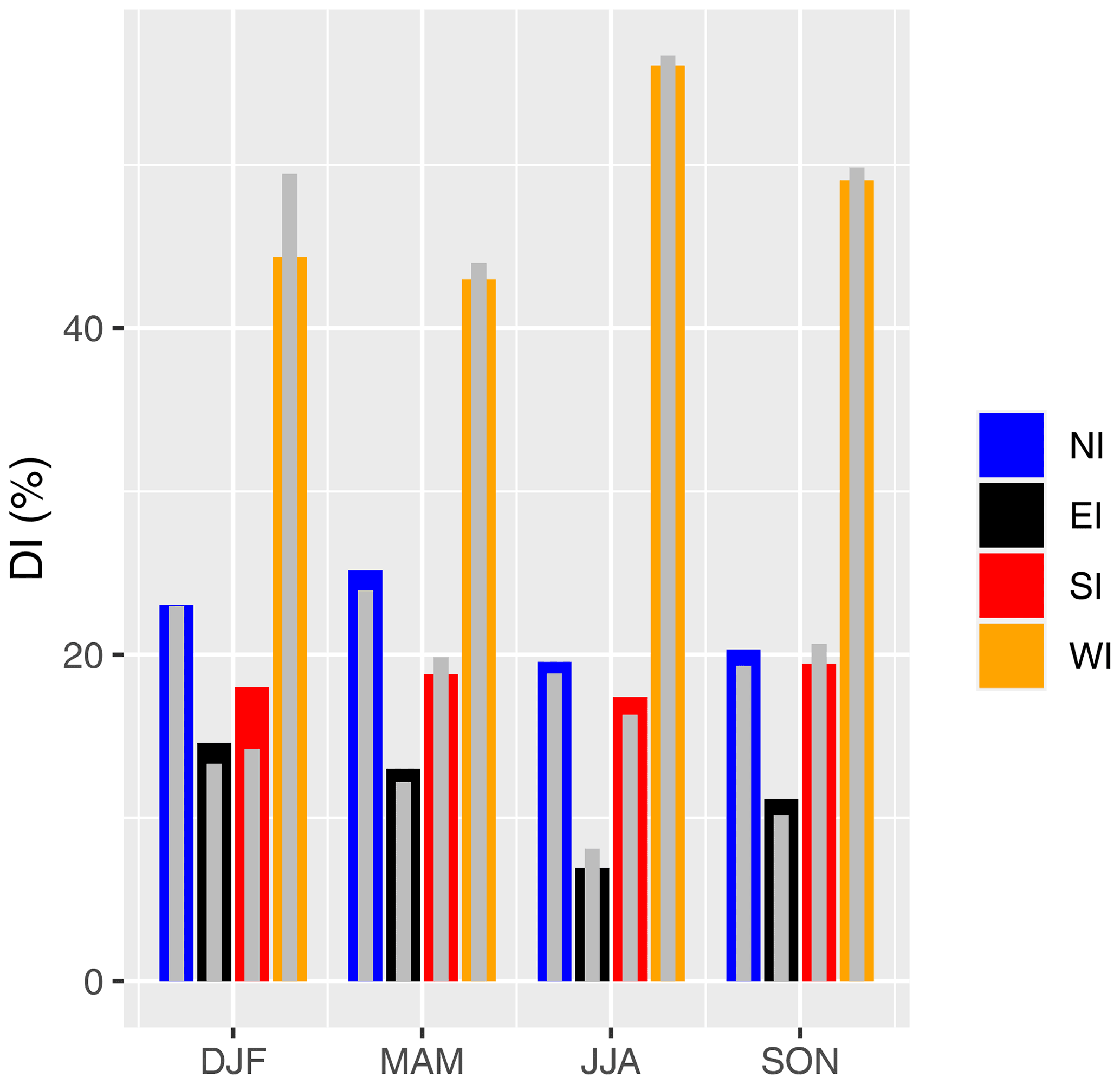
Figure 10Seasonal frequencies of directional indices (DI: NI, EI, SI, and WI in percentage of nonmissing days) averaged for the period of 1665–1713 (color bars). Thin gray bars indicate the corresponding values for the 1981–2010 reference period (ERA5 data).
For both periods, the WI is the most recurrent DI, indicating predominance in the region of westerly movement of the clouds. The frequency of days with meridional circulation (the sum of SI and NI) during the LMM was slightly higher than during the reference period, and the WI is characterized by lower frequencies in the LMM than in the reference period for all seasons. As shown by Barriopedro et al. (2014), a below-normal persistence of westerlies inhibits the warm oceanic advection over most of Europe during all seasons, except in summer, when it is rather associated with high-pressure systems and radiative warming. In terms of precipitation, the WI is an optimal indicator for the transport of moisture fluxes to Europe, with decreased westerlies corresponding to below-average precipitation over large areas of central Europe all year-round (Barriopedro et al., 2014). Accordingly, the reduced frequency of WI in Fig. 10 indicates a drier and colder DJF, as well as a moderate MAM, JJA, and SON in terms of precipitation and temperature compared to present (with the exception of summer). As seen earlier, this statement is true for DJF, MAM, and JJA, but SON was cooler with respect to the reference period (Fig. 5).
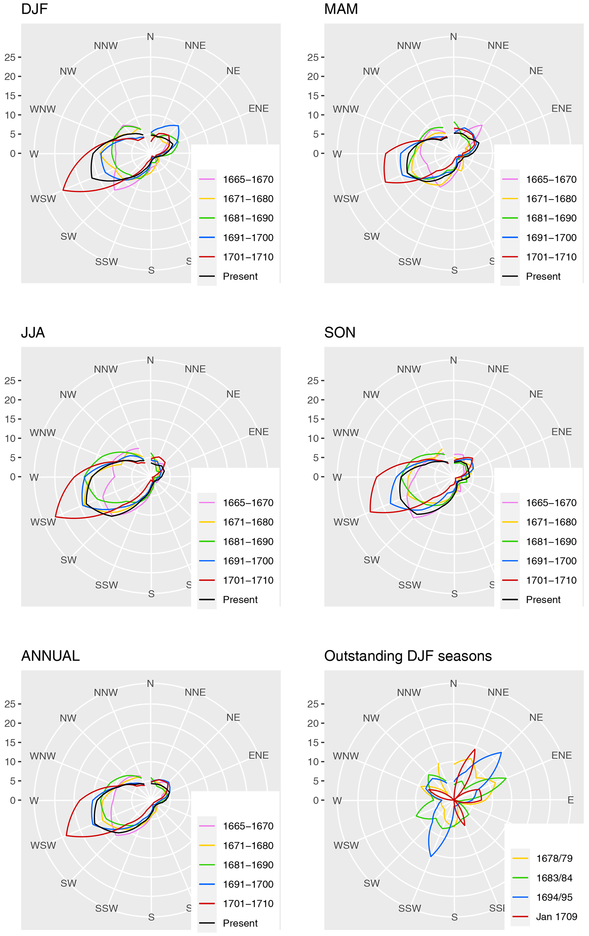
Figure 11Visualization of DIs (in percentage of total days) as a seasonal mean (DJF, MAM, JJA, SON), as an annual mean, for outstanding DJF seasons, and for January 1709.
With the aim of analyzing the variability of the decades, we looked at the wind roses of the different seasons (Fig. 11). To ensure comparability, the mean values of ERA5 (1981–2010) are also plotted. The strongest deviation from the current time shows the decade 1701–1710, which is characterized by high percentage values in the W and WSW sectors. The decade 1691–1700 shows a different picture, with high percentage values in the NNE, NE, and ENE sectors noted in DJF, while in the other seasons only small deviations from the current time are seen. It is also worth mentioning that the 2 decades 1671–1690 show a strong decrease in airflows from the westerly direction. In addition, a strong interdecadal variability can be seen. An interesting picture is shown by the wind roses of the exceptional winters in the LMM. The winter of 1679 is characterized by low W values and high values in the N and NE direction. The winter of 1694/95 shows a similar picture, whereas the winter of 1683/84 shows a moderate distribution but with a pronounced E direction. January 1709 is characterized by a strong NNE direction and weaker expressions of ENE, E, SSE, and WNW. So, January shows a circulation structure, which leads to cold temperatures, whereas, looking at the whole winter of 1708/09, the dominant direction of movement of the clouds is the WSW direction with a percentage of 36 %. This illustrates the contrast of the individual months in the winter of 1708/09 with respect to the circulation situation and, subsequently, the temperatures.
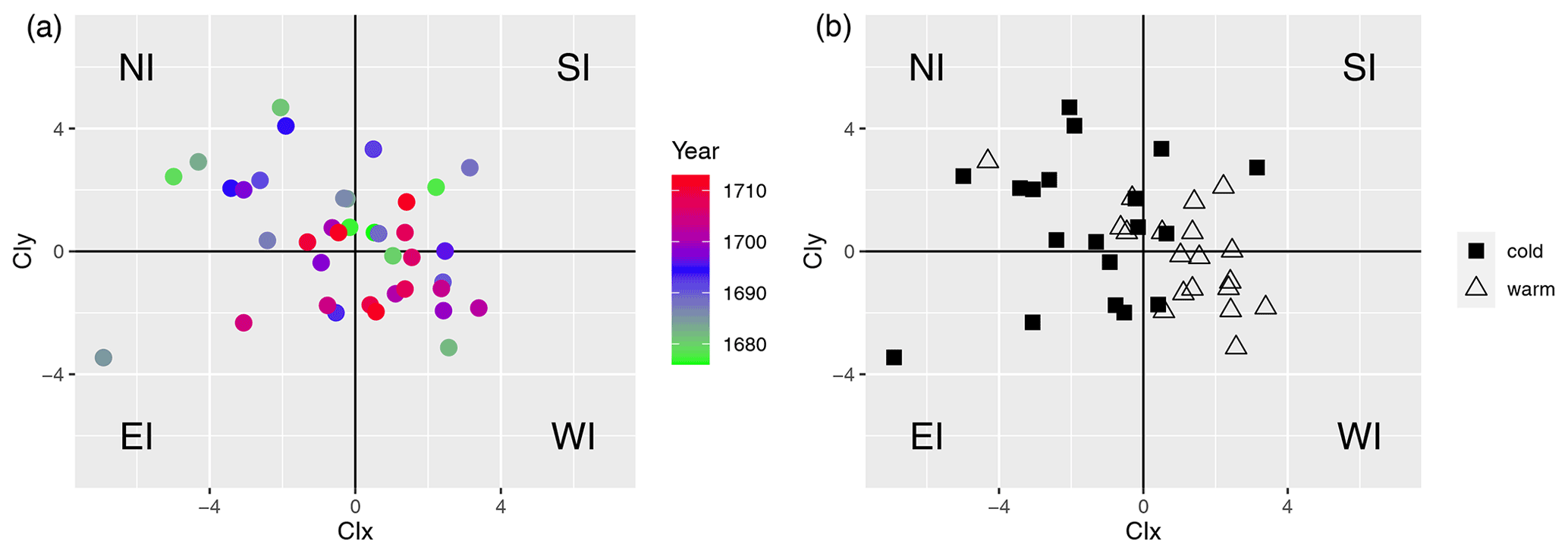
Figure 12(a) Scatterplot of the CI for the LMM winters, with colors indicating the year within the LMM. The x axis represents the CIx coordinate of the CI and the y axis the CIy coordinate of the CI. (b) As in panel (a) but showing two different clusters; squares are below the median of Tmean and triangles are above the median of Tmean.
To characterize the interannual circulation variability within the LMM and synthesize the four-dimensional information on the DIs, we computed a cumulative circulation index (CI; Mellado-Cano et al., 2018) that aggregates the standardized values ()) of the four DIs in two components (CIx, CIy):
The component CIx is purely based on atmospheric circulation but it can also be used as an indicator of the European temperature conditions that could be expected from the dynamics, with positive values of CIx indicating an overall warming and negative values of CIx indicating an overall cooling. CIy measures the degree of meridional (NI, SI) versus zonal (WI, EI) circulation, with positive values indicating a dominance of the former and negative values indicating a dominance of the latter. The results are shown in Fig. 12 and the standardized time series of DI separated into seasons can be seen in the Appendix (Figs. A4–A7). The left-hand plot shows a scatterplot with a color marking of the different years. Again, the decade 1701–1710 (red dots) shows a shift towards WI, while the decade 1691–1700 is relatively scattered, indicating high variability but with a tendency towards NI. In the right-hand panel, squares represent cold winters and triangles represent warm winters. The separator of the warm and cold winter seasons is the median of the Morin time series. This plot can be seen as an internal validation of the Morin data. Warm winters imply a tendency towards WI, while cold winters show a tendency towards NI. The relationship of WI and mean temperature can be read in Fig. A8, which is approximately 1∘ per 10 %. This shows that large-scale weather conditions can explain at least part of the cooling in the winter months.
We have digitized three meteorological variables (i.e., temperature, direction of the movement of the clouds, and cloud cover) from copies of Louis Morin's original measurements (source: Institute of History/Oeschger Centre for Climate Change Research, University of Bern, 1665–1709; Institut de France, 1710–1713) and subjected them to quality analysis to make these data available to the scientific community. Our available data cover the period 1665–1713 (temperature beginning in 1676). Thus, during this time period, three values are available on a daily basis for each variable: morning, midday/afternoon, and evening. Hypotheses about largely unavailable metadata for the temperature measurements were supported with statistical tests and by drawing on proxy data. Only small irregularities were uncovered in the data, and they are therefore considered trustworthy with respect to the possibilities at that time. In addition, Morin's measurements have a high correlation with grape harvest dates (GHDs) and show a snowfall frequency threshold of 1.5 ∘C, which is an indicator of the lower calibration point of the thermometer. An analysis of the variables examined here shows internal consistency and may thus be useful in further describing the Late Maunder Minimum (LMM). However, we discussed two possible inhomogeneities of the temperature, which are provided as an additional homogenized time series of the temperature in the data file. The main statements of this paper are not affected by these potential inhomogeneities.
The LMM, which is defined by observed exceptionally low sunspot numbers, is considered an exceptionally cold period of the Little Ice Age (LIA). However, seasonal temperatures reveal a more differentiated picture of a high frequency of cold winters and falls but is close to modern values in springs and summers (see Fig. 5). The highest numbers of cold winters occur in the decade 1691–1700. Previous studies show that the main causes include volcanic activities, the reduction of the total solar irradiance (decrease in sunspots), and a multicentennial reduction in the northward heat transport by the subpolar gyre. With the data of Morin we cannot make strong statements about an attribution. However, we have shown the following: in this period, winter months show a significant lower frequency of the westerly direction in the movement of the clouds (see Fig. 10). This reduction of advection from the ocean leads to cooling in Paris in winter. This can be seen very clearly when comparing the last decade of the 17th century (cold) and the first decade of the 18th century (warm) (see Fig. 9). A drop in the frequency of the westerly index (WI) between 1691 and 1700 is followed by a rise in WI in the first decade of the 18th century. A lower frequency of the westerly direction in the movement of the clouds can also be seen in summer, and this reduction probably leads to moderate to warm temperatures in summer. Thus, unusually cold winters in the LMM can be partly attributed to a lower frequency of the westerly direction in the movement of the clouds and a rise in either the northerly index (NI) or easterly index (EI). This is shown in Fig. 12, where outstanding cold winters coincide with a low WI. Interestingly, the notorious winter of 1708/09 is not particularly pronounced in terms of mean temperature because December 1708 was moderate, and devastatingly cold temperatures (up to −18 ∘C) were restricted to January. This contrast is also reflected in the analysis of the movement of the air, wherein the WSW direction is dominant for DJF 1708/09 and NNE and E are dominant for January 1709, so in terms of temperature, a moderate December and February weakens indices concerning the whole winter of 1708/09.
An impact analysis reveals that the winter of 1708/09 was indeed a devastating winter with respect to consecutive ice days. Although in terms of consecutive cold days the winters of 1676/77, 1678/79, 1683/84, 1692/93, 1694/95, and 1696/97 are more pronounced. The absolute number of cold days and ice days is highest in the last decade of the 17th century (exceptional winters: 1690/91, 1691/92, 1694/95, and 1696/97).
An investigation of the cloud cover data revealed high discrepancies with respect to modern values, with the winter season (DJF, −14.0 %), the spring season (MAM, −20.8 %), the summer season (JJA, −17.9 %), and the fall season (SON, −18.0 %) showing a negative anomaly of TCC. Thus, the subjective measurement of cloud cover in quantitative terms should be taken with caution. In summary, Morin's measurements are characterized by an extraordinary long duration (1665–1713) and continuity, and they are therefore a good source to get a comprehensive picture of the regional climate in Paris in the LMM. Therefore, we will investigate some further variables (precipitation and humidity), which will provide further insights into the climate in Paris during the late 17th and early 18th century.
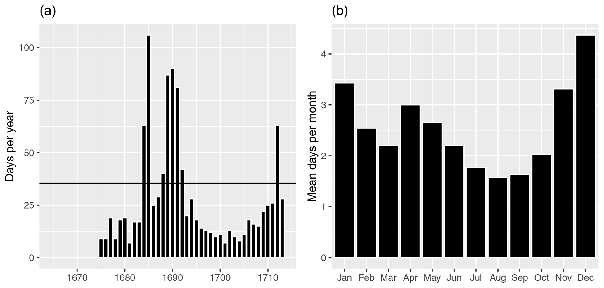
Figure A1In panel (a) the total number of days when the evening temperature exceeds the midday/afternoon temperature is shown. The black horizontal line represents the mean value of the ERA5 data from 1981 to 2010. In panel (b) the frequency of days when the evening temperature exceeds the midday/afternoon temperature (per month) is shown.

Figure A2In panel (a) the mean DTR per month of the E-OBS data, of the different locations, and of the whole time period can be seen. In panel (b) the yearly mean DTR is plotted, and the horizontal line represents the mean of the reference period from 1961 to 1990 (E-OBS).
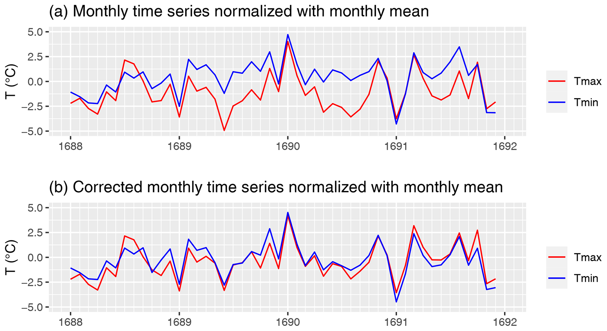
Figure A3Tmin and Tmax normalized with monthly mean values of 1688–1691. In panel (a) are the monthly mean values of Morin's measurements and in panel (b) the homogenized measurements.
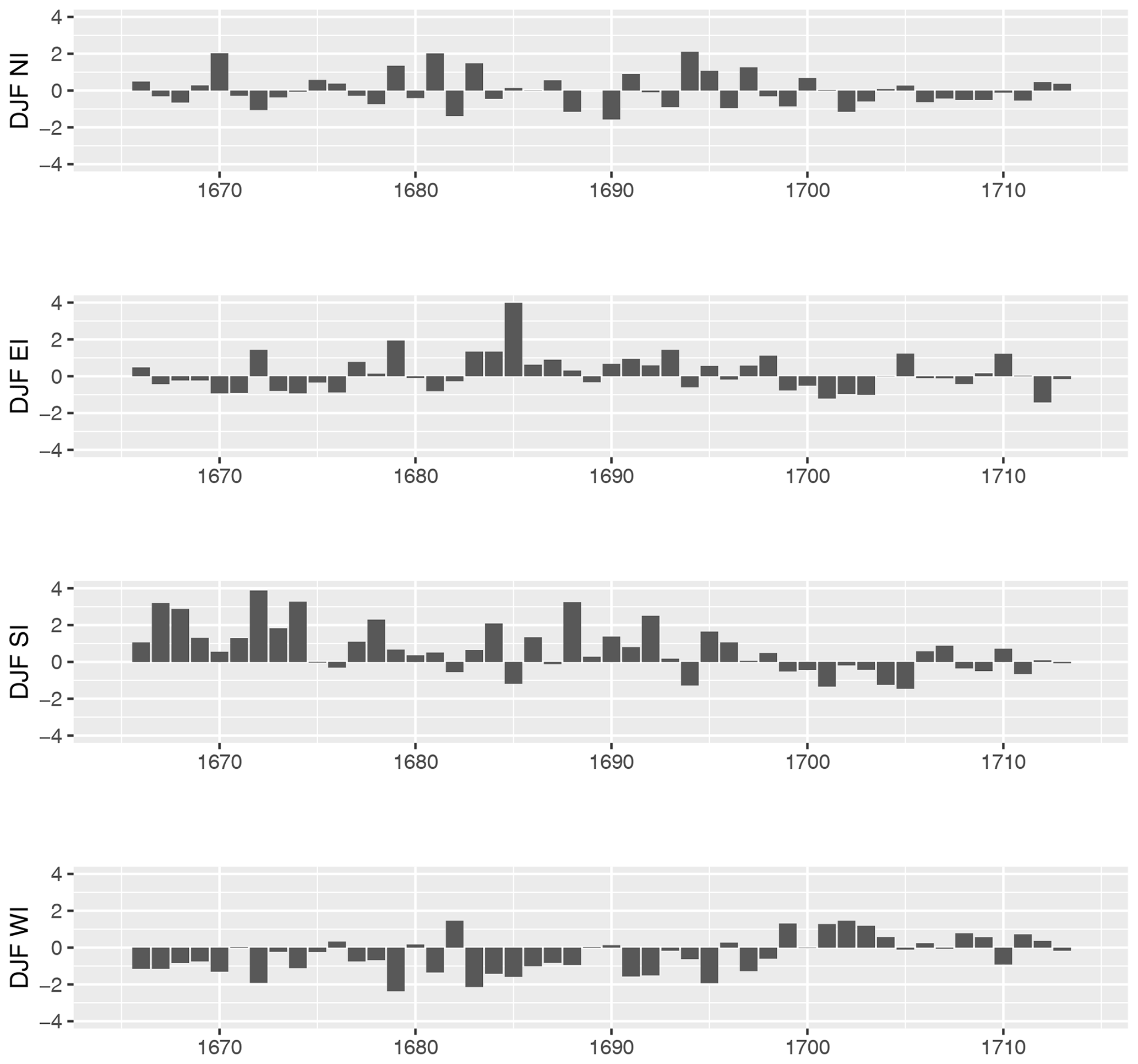
Figure A4Standardized DJF DI time series for the LMM (1665–1713) with respect to the mean of the reference period of 1981–2010.
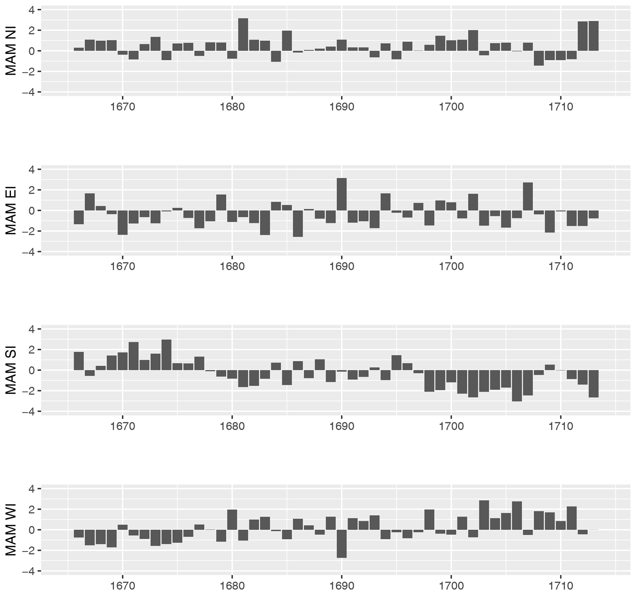
Figure A5Standardized MAM DI time series for the LMM (1665–1713) with respect to the mean of the reference period of 1981–2010.

Figure A6Standardized JJA DI time series for the LMM (1665–1713) with respect to the mean of the reference period of 1981–2010.
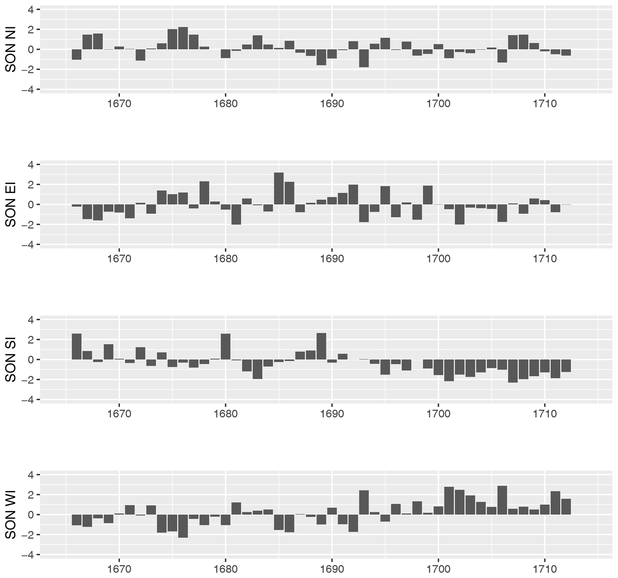
Figure A7Standardized SON DI time series for the LMM (1665–1713) with respect to the mean of the reference period of 1981–2010.

Figure A8The correlation of the WI with the mean temperature in Paris (ERA5; 1981–2010), a linear regression (red line) over all data points, and a linear regression (green line) excluding outstanding and/or extraordinary years (1985, 1986, 1987, and 2010).
All the data used to perform the analysis in this study are described and properly referenced in the paper. The supplementary dataset can be found here: https://doi.org/10.5281/zenodo.6565771 (Pliemon et al., 2022).
We adopted quality-assured hourly and monthly data from ERA5 (1979–present) to compare the direction of the movements of the clouds and the cloudiness to contemporary conditions (ERA5 pressure levels hourly: Hersbach et al., 2018a, https://doi.org/10.24381/cds.bd0915c6; ERA5 single levels monthly: Hersbach et al., 2019, https://doi.org/10.24381/cds.f17050d7). We chose a reference period of 30 years as suggested by the WMO (2003, https://library.wmo.int/index.php?lvl=notice_display&id=11635#.Ys15HtPP1PY, last access: 1 July 2022) from 1981 to 2010. Furthermore, we used hourly ERA5 data on temperature and precipitation to statistically analyze the measurement times of Morin and to validate the thermometer (ERA5 single levels hourly: Hersbach et al., 2018b, https://doi.org/10.24381/cds.adbb2d47). As a reference period for the temperature data, we used the observations of E-OBS version 21.0e (Cornes et al., 2018, https://doi.org/10.1029/2017JD028200) for the common period from 1961 to 1990. Furthermore, we included in our study the grape harvest dates (GHDs) from Beaune (Labbé et al., 2019, https://doi.org/10.5194/cp-15-1485-2019), the Central England Temperature (CET, Manley, 1974, https://doi.org/10.1002/qj.49710042511), and winter temperatures from De Bilt (Van Den Dool et al., 1978, https://doi.org/10.1007/BF00135153).
Thomas Pliemon was responsible for conceptualization, data curation, formal analysis, investigation, methodology, resources, software, validation, visualization, and writing (original draft preparation as well as review and editing). Ulrich Foelsche was responsible for conceptualization, funding acquisition, project administration, resources, supervision, validation, and writing (review and editing). Christian Rohr was responsible for resources, validation, and writing (review and editing). Christian Pfister was responsible for resources, validation, and writing (review and editing).
The contact author has declared that neither they nor their co-authors have any competing interests.
The results contain modified Copernicus Climate Change Service information from 2022. Neither the European Commission nor ECMWF is responsible for any use that may be made of the Copernicus information or data it contains.
Publisher's note: Copernicus Publications remains neutral with regard to jurisdictional claims in published maps and institutional affiliations.
We acknowledge the E-OBS dataset from the EU-FP6 project UERRA (http://www.uerra.eu/, last access: 15 March 2022) and the Copernicus Climate Change Service, as well as the data providers in the ECA&D project (https://www.ecad.eu/, last access: 15 March 2022).
We also acknowledge the Copernicus Climate Change Service (C3S) Climate Data Store for Hersbach et al. (2018a, b, 2019).
This research has been supported by the Austrian Science Fund (grant no. Clim_Hist_LIA P31088-N29).
This paper was edited by Jürg Luterbacher and reviewed by two anonymous referees.
Alcoforado, M.-J., de Fátima Nunes, M., Garcia, J. C., and Taborda, J. P.: Temperature and precipitation reconstruction in southern Portugal during the late Maunder Minimum (AD 1675–1715), The Holocene, 10, 333–340, https://doi.org/10.1191/095968300674442959, 2000. a
Alcoforado, M. J., Vaquero, J. M., Trigo, R. M., and Taborda, J. P.: Early Portuguese meteorological measurements (18th century), Clim. Past, 8, 353–371, https://doi.org/10.5194/cp-8-353-2012, 2012. a
Barriendos, M.: Climatic variations in the Iberian Peninsula during the late Maunder Minimum (AD 1675-1715): an analysis of data from rogation ceremonies, The Holocene, 7, 105–111, https://doi.org/10.1177/095968369700700110, 1997. a
Barriopedro, D., García-Herrera, R., and Huth, R.: Solar modulation of Northern Hemisphere winter blocking, J. Geophys. Res., 113, D14118, https://doi.org/10.1029/2008JD009789, 2008. a
Barriopedro, D., Gallego, D., Alvarez-Castro, M. C., García-Herrera, R., Wheeler, D., Peña-Ortiz, C., and Barbosa, S. M.: Witnessing North Atlantic westerlies variability from ships’ logbooks (1685–2008), Clim. Dynam., 43, 939–955, https://doi.org/10.1007/s00382-013-1957-8, 2014. a, b, c, d
Brandsma, T. and van der Meulen, J. P.: Thermometer screen intercomparison in De Bilt (the Netherlands) – Part II: description and modeling of mean temperature differences and extremes, Int. J. Climatol., 28, 389–400, https://doi.org/10.1002/joc.1524, 2008.
Böhm, R., Jones, P. D., Hiebl, J., Frank, D., Brunetti, M., and Maugeri, M.: The early instrumental warm-bias: a solution for long central European temperature series 1760–2007, Climatic Change, 101, 41–67, https://doi.org/10.1007/s10584-009-9649-4, 2010. a, b
Camuffo, D.: Errors in Early Temperature Series Arising from Changes in Style of Measuring Time, Sampling Schedule and Number of Observations, Climatic Change, 53, 331–352, https://doi.org/10.1023/A:1014962623762, 2002. a
Camuffo, D. and Bertolin, C.: The earliest temperature observations in the world: the Medici Network (1654–1670), Climatic Change, 111, 335–363, https://doi.org/10.1007/s10584-011-0142-5, 2012. a
Camuffo, D. and della Valle, A.: A summer temperature bias in early alcohol thermometers, Climatic Change, 138, 633–640, https://doi.org/10.1007/s10584-016-1760-8, 2016. a, b, c
Camuffo, D., Bertolin, C., Jones, P. D., Cornes, R., and Garnier, E.: The earliest daily barometric pressure readings in Italy: Pisa AD 1657–1658 and Modena AD 1694, and the weather over Europe, The Holocene, 20, 337–349, 2010. a
Camuffo, D., della Valle, A., Bertolin, C., and Santorelli, E.: Temperature observations in Bologna, Italy, from 1715 to 1815: a comparison with other contemporary series and an overview of three centuries of changing climate, Climatic Change, 142, 7–22, https://doi.org/10.1007/s10584-017-1931-2, 2017. a
Camuffo, D., della Valle, A., Becherini, F., and Rousseau, D.: The earliest temperature record in Paris, 1658–1660, by Ismaël Boulliau, and a comparison with the contemporary series of the Medici Network (1654–1670) in Florence, Climatic Change, 162, 903–922, https://doi.org/10.1007/s10584-020-02756-9, 2020. a
Camuffo, D., della Valle, A., and Becherini, F.: From time frames to temperature bias in temperature series, Climatic Change, 165, 38, https://doi.org/10.1007/s10584-021-03065-5, 2021. a
Chambers, F. M., Brain, S. A., Mauquoy, D., McCarroll, J., and Daley, T.: The ‘Little Ice Age’ in the Southern Hemisphere in the context of the last 3000 years: Peat-based proxy-climate data from Tierra del Fuego, The Holocene, 24, 1649–1656, https://doi.org/10.1177/0959683614551232, 2014. a
Chuine, I., Yiou, P., Viovy, N., Seguin, B., Daux, V., and Ladurie, E. L. R.: Grape ripening as a past climate indicator, Nature, 432, 289–290, https://doi.org/10.1038/432289a, 2004. a, b, c
Copernicus Climate Change Service (C3S): ERA5: Fifth generation of ECMWF atmospheric reanalyses of the global climate, Copernicus Climate Service Climate Data Store (CDS), https://cds.climate.copernicus.eu/cdsapp#!/home (last access: 5 April 2022), 2017.
Cornes, R. C.: Early Meteorological Data from London and Paris Extending the North Atlantic Oscillation Series, PhD thesis, University of East Anglia, 2010. a, b
Cornes, R. C., Jones, P. D., Briffa, K. R., and Osborn, T. J.: A daily series of mean sea-level pressure for Paris, 1670–2007, Int. J. Climatol., 32, 1135–1150, https://doi.org/10.1002/joc.2349, 2012. a, b, c
Cornes, R. C., van der Schrier, G., van den Besselaar, E. J. M., and Jones, P.: An Ensemble Version of the E-OBS Temperature and Precipitation Datasets, J. Geophy. Res.-Atmos., 123, 9391–9409, https://doi.org/10.1029/2017JD028200, 2018. a, b
Cox, D. T. C., Maclean, I. M. D., Gardner, A. S., and Gaston, K. J.: Global variation in diurnal asymmetry in temperature, cloud cover, specific humidity and precipitation and its association with leaf area index, Glob. Change Biol., 26, 7099–7111, https://doi.org/10.1111/gcb.15336, 2020. a
Dai, A.: Temperature and pressure dependence of the rain-snow phase transition over land and ocean, Geophys. Res. Lett., 35, L12802, https://doi.org/10.1029/2008GL033295, 2008. a
Dai, A., Trenberth, K. E., and Karl, T. R.: Effects of clouds, soil moisture, precipitation, and water vapor on diurnal temperature range, J. Climate, 12, 2451–2473, https://doi.org/10.1175/1520-0442(1999)012<2451:EOCSMP>2.0.CO;2, 1999. a
Daux, V., Garcia de Cortazar-Atauri, I., Yiou, P., Chuine, I., Garnier, E., Le Roy Ladurie, E., Mestre, O., and Tardaguila, J.: An open-access database of grape harvest dates for climate research: data description and quality assessment, Clim. Past, 8, 1403–1418, https://doi.org/10.5194/cp-8-1403-2012, 2012. a, b, c, d
de Fontenelle, B. L. B.: Histoire de l'Académie royale des sciences, chap. Éloge de M. Morin, 1715 (in French). a, b, c
Delaunay, P.: Vieux médecins sarthois. Première série, Jean de L'Épine; J. Aubert; F. Cureau de La Chambre; B. Dieuxivoye; La Fontaine et les médecins : la querelle du quinquina; de Dieuxivoye à Blégny; L. Morin; F. Poupart; Lepelletier de la Sarthe; Dominique Peffault de Latour; Guy Patin et Jean Bineteau, 1906 (in French). a
Diodato, N., Bellocchi, G., Bertolin, C., and Camuffo, D.: Climate variability analysis of winter temperatures in the central Mediterranean since 1500 AD, Theor. Appl. Climatol., 116, 203–210, https://doi.org/10.1007/s00704-013-0945-6, 2014. a
Grove, J. M.: Little Ice Ages – Ancient and Modern, vol. I, Routledge, London, 2nd edn., ISBN 0-415-33422-5, 2004. a
Hahn, C. J., Rossow, W. B., and Warren, S. G.: ISCCP cloud properties associated with standard cloud types identified in individual surface observations, J. Climate, 14, 11–21, https://doi.org/10.1175/1520-0442(2001)014<0011:ICPAWS>2.0.CO;2, 2001. a
Hersbach, H., Bell, B., Berrisford, P., Biavati, G., Horányi, A., Muñoz Sabater, J., Nicolas, J., Peubey, C., Radu, R., Rozum, I., Schepers, D., Simmons, A., Soci, C., Dee, D., and Thépaut, J.-N.: ERA5 hourly data on pressure levels from 1979 to present, Copernicus Climate Change Service (C3S) Climate Data Store (CDS) [data set], https://doi.org/10.24381/cds.bd0915c6, 2018a. a, b, c
Hersbach, H., Bell, B., Berrisford, P., Biavati, G., Horányi, A., Muñoz Sabater, J., Nicolas, J., Peubey, C., Radu, R., Rozum, I., Schepers, D., Simmons, A., Soci, C., Dee, D., and Thépaut, J.-N.: ERA5 hourly data on single levels from 1979 to present, Copernicus Climate Change Service (C3S) Climate Data Store (CDS) [data set], https://doi.org/10.24381/cds.adbb2d47, 2018b. a, b, c
Hersbach, H., Bell, B., Berrisford, P., Biavati, G., Horányi, A., Muñoz Sabater, J., Nicolas, J., Peubey, C., Radu, R., Rozum, I., Schepers, D., Simmons, A., Soci, C., Dee, D., and Thépaut, J.-N.: ERA5 monthly averaged data on single levels from 1979 to present, Copernicus Climate Change Service (C3S) Climate Data Store (CDS) [data set], https://doi.org/10.24381/cds.f17050d7, 2019. a, b, c
Jennings, K., Winchell, T., Livneh, B., and Molotch, N.: Spatial variation of the rain snow temperature threshold across the Northern Hemisphere, Nat. Commun., 9, 1148, https://doi.org/10.1038/s41467-018-03629-7, 2018. a, b
Jones, P. D.: Classics in physical geography revisited, Prog. Phys. Geogr., 23, 425–428, 1999. a
Können, G. P. and Brandsma, T.: Instrumental pressure observations from the end of the 17th Century: Leiden (The Netherlands), Int. J. Climatol., 25, 1139–1145, 2005. a
Labbé, T., Pfister, C., Brönnimann, S., Rousseau, D., Franke, J., and Bois, B.: The longest homogeneous series of grape harvest dates, Beaune 1354–2018, and its significance for the understanding of past and present climate, Clim. Past, 15, 1485–1501, https://doi.org/10.5194/cp-15-1485-2019, 2019. a, b, c, d, e, f
Lambert, C.-F.: Histoire littéraire du règne de Louis XIV, Prault, Paris, 1751 (in French). a
Legrand, J.-P. and Le Goff, M.: Louis Morin et les observations météorologiques sous Louis XIV, La Vie des Sciences, 4, 251–281, 1987 (in French). a, b, c, d, e, f, g, h, i, j, k, l, m, n, o
Legrand, J.-P. and Le Goff, M.: Les observations météorologiques de Louis Morin, Direction de la météorologie nationale, Paris, 1992 (in French). a, b, c, d, e, f
Legrand, J.-P., Le Goff, M., and Mazaudier, C.: On the climatic changes and the sunspot activity during 17th century, Ann. Geophys., 8, 637–644, 1990. a
Legrand, J.-P., Le Goff, M., Mazaudier, C., and Schröder, W.: Solar and auroral activities during the Seventeenth Century, Acta. Geod. Geoph. Mont. Hung., 27, 251–282, 1992. a, b, c
Lockwood, M., Owens, M., Hawkins, E., Jones, G. S., and Usoskin, I.: Frost fairs, sunspots and the Little Ice Age, Astron. Geophys., 58, 2.17–2.23, https://doi.org/10.1093/astrogeo/atx057, 2017. a, b, c
Luterbacher, J.: The Late Maunder Minimum (1675–1715) — Climax of the ‘Little Ice Age’ in Europe, in: History and Climate, edited by: Jones, P. D., Ogilvie, A. E. J., Davies, T. D., and Briffa, K. R., Springer, Boston, MA, https://doi.org/10.1007/978-1-4757-3365-5_3, 2001. a
Luterbacher, J., Rickli, R., Tinguely, C., Xoplaki, E., Schüpbach, E., Dietrich, D., Hüsler, J., Ambühl, M., Pfister, C., Beeli, P., Dietrich, U., Dannecker, A., Davies, T., Jones, P., Slonosky, V., Ogilvie, A., Maheras, P., Kolyva-Machera, F., Martin-Vide, J., Barriendos, M., Alcoforado, M., Nunes, M., Jónsson, T., Glaser, R., Jacobeit, J., Beck, C., Philipp, A., Beyer, U., Kaas, E., Schmith, T., Bärring, L., Jönsson, P., Rácz, L., and Wanner, H.: Monthly mean pressure reconstruction for the Late Maunder Minimum Period (AD 1675–1715), Int. J. Climatol., 20, 1049–1066, https://doi.org/10.1002/1097-0088(200008)20:10<1049::AID-JOC521>3.0.CO;2-6, 2000. a, b
Luterbacher, J., Rickli, R., Xoplaki, E., Tinguely, C., Beck, C., Pfister, C., and Wanner, H.: The Late Maunder Minimum (1675–1715) – A key period for studying decadal scale climatic change in Europe, Climatic Change, 49, 441–462, https://doi.org/10.1023/A:1010667524422, 2001. a, b
Mace, G. G., Benson, S., and Kato, S.: Cloud radiative forcing at the Atmospheric Radiation Measurement Program Climate Research Facility: 2. Vertical redistribution of radiant energy by clouds, J. Geophys. Res., 111, D11S91, https://doi.org/10.1029/2005JD005922, 2006. a
Manley, G.: Central England temperatures: Monthly means 1659 to 1973, Q. J. Roy. Meteor. Soc., 100, 389–405, https://doi.org/10.1002/qj.49710042511, 1974. a, b, c
Mann, M. E., Zhang, Z., Rutherford, S., Bradley, R. S., Hughes, M. K., Shindell, D., Ammann, C., Faluvegi, G., and Ni, F.: Global signatures and dynamical origins of the Little Ice Age and Medieval Climate Anomaly, Science, 326, 1256–1260, https://doi.org/10.1126/science.1177303, 2009. a
Matthews, J. A. and Briffa, K. R.: The ‘LitleE Ice Age’: Re-evaluation of an evolving concept, Geogr. Ann. A, 87, 17–36, https://doi.org/10.1111/j.0435-3676.2005.00242.x, 2005. a
Meier, N., Rutishauser, T., Pfister, C., Wanner, H., and Luterbacher, J.: Grape harvest dates as a proxy for Swiss April to August temperature reconstructions back to AD 1480, Geophys. Res. Lett., 34, L20705, https://doi.org/10.1029/2007GL031381, 2007. a, b, c
Mellado-Cano, J., Barriopedro, D., García-Herrera, R., Trigo, R. M., and Álvarez Castro, M. C.: Euro-Atlantic atmospheric circulation during the Late Maunder Minimum, J. Climate, 31, 3849–3863, https://doi.org/10.1175/JCLI-D-17-0261.1, 2018. a, b, c, d, e, f, g, h
Menzel, A.: A 500 year pheno-climatological view on the 2003 heatwave in Europe assessed by grape harvest dates, Meteorol. Z., 14, 75–77, 2005. a
Moreno-Chamarro, E., Zanchettin, D., Lohmann, K., Luterbacher, J., and Jungclaus, J. H.: Winter amplification of the European Little Ice Age cooling by the subpolar gyre, Scientific Reports, 7, 9981, https://doi.org/10.1038/s41598-017-07969-0, 2017. a
Neukom, R., Steiger, N., Gómez-Navarro, J. J., Wang, J., and Werner, J. P.: No evidence for globally coherent warm and cold periods over the preindustrial Common Era, Nature, 571, 550–554, https://doi.org/10.1038/s41586-019-1401-2, 2019. a
Niedźwiedź, T.: Summer Temperatures in the Tatra Mountains During the Maunder Minimum (1645–1715),, Springer Netherlands, Dordrecht, 397–406 https://doi.org/10.1007/978-90-481-3167-9_19, 2010. a
Pfister, C.: Wetternachhersage: 500 Jahre Klimavariationen und Naturkatastrophen, Verlag Paul Haupt, Bern/Stuttgart/Wien, ISBN 3-258-05696-x, 1999. a
Pfister, C.: Klimawandel in der Geschichte Europas, Österreichische Zeitschrift für Geschichtswissenschaften, 12, 7–43, 2001. a
Pfister, C.: Historical Records as Evidence in the Climate Change Debate, in: Effect of Climate Change on Built Environment, edited by: Bunnik, T., De Clercq, H., van Hees, R. P. J., Schellen, H. L., and Schueremans, L., WTA-Schriftenreihe, München, wissenschaftlich-Technische Arbeitsgemeinschaft für Bauwerkserhaltung und Denkmalpflege, 34, 5–16, 2010. a
Pfister, C. and Bareiss, W.: The climate in Paris between 1675 and 1715 according to the Meteorological Journal of Louis Morin, in: Climatic trends and anomalies in Europe 1675–1715: High resolution spatio-temporal reconstructions from direct meteorological observations and proxy data. Methods and results, edited by: Frenzel, B., Pfister, C., and Gläser, B., Gustav Fischer Verlag, Stuttgart, Jena, New York, 151–171, 1994. a, b, c, d, e, f, g
Pfister, C. and Wanner, H.: Climate and Society in Europe. The Last Thousand Years, Haupt, Bern, ISBN 978-3-258-08234-9, 2021. a
Pliemon, T., Foelsche, U., Rohr, C., Pfister, C.: Subdaily meteorological measurements of temperature, direction of the movement of the clouds, and cloud cover in the Late Maunder Minimum by Louis Morin in Paris, Zenodo [data set], https://doi.org/10.5281/zenodo.6565771, 2022. a
Rácz, L.: The climate of Hungary during the Late Maunder Minimum (1675–1715), in: Climatic trends and anomalies in Europe 1675–1715: High resolution spatio-temporal reconstructions from direct meteorological observations and proxy data. Methods and results, edited by: Frenzel, B., Pfister, C., and Gläser, B., Gustav Fischer Verlag, Stuttgart, Jena, New York, 151–171, 1994. a
Rhodes, R. H., Bertler, N. A. N., Baker, J. A., Steen-Larsen, H. C., Sneed, S. B., Morgenstern, U., and Johnsen, S. J.: Little Ice Age climate and oceanic conditions of the Ross Sea, Antarctica from a coastal ice core record, Clim. Past, 8, 1223–1238, https://doi.org/10.5194/cp-8-1223-2012, 2012. a
Rousseau, D.: Les températures mensuelles en région parisienne de 1676 à 2008, La Météorologie, 67, 43–55, https://doi.org/10.4267/2042/30038, 2009 (in French). a, b, c, d, e
Rousseau, D.: Les moyennes mensuelles de températures á Paris de 1658 à 1675 d'Ismail Boulliau à Louis Morin, La Météorologie, 81, 11–22, 2013 (in French). a, b
Sanchez-Lorenzo, A., Calbó, J., and Wild, M.: Increasing cloud cover in the 20th century: review and new findings in Spain, Clim. Past, 8, 1199–1212, https://doi.org/10.5194/cp-8-1199-2012, 2012. a, b
Slonosky, V., Jones, P., and Davies, T.: Instrumental pressure observations and atmospheric circulation from the 17th and 18th Centuries: London and Paris, Int. J. Climatol., 21, 285–298, https://doi.org/10.1002/joc.611, 2001. a, b
Sun, B., Groisman, P. Y., Bradley, R. S., and Keimig, F. T.: Temporal Changes in the Observed Relationship between Cloud Cover and Surface Air Temperature, J. Climate, 13, 4341–4357, https://doi.org/10.1175/1520-0442(2000)013<4341:TCITOR>2.0.CO;2, 2000. a
Van Den Dool, H. M., Krijnen, H. J., and Schuurmans, C. J. E.: Average winter temperatures at De Bilt (the Netherlands): 1634–1977, Climatic Change, 1, 319–330, https://doi.org/10.1007/BF00135153, 1978. a, b
van der Meulen, J. P. and Brandsma, T.: Thermometer screen intercomparison in De Bilt (The Netherlands), Part I: Understanding the weather-dependent temperature differences), Int. J. Climatol., 28, 371–387, https://doi.org/10.1002/joc.1531, 2008.
Visscher, J. C.: Lutetia Parisiorum urbs, toto orbe celeberrima notissimaque, caput Regni Franciae, Bibliotheque Nationale de France, Paris, Bibliothèque nationale de France, https://gallica.bnf.fr/ (last access: 4 January 2022), 1618. a
Wanner, H., Hurrell, J. W., Kushnir, Y., Ottersen, G., and Visbeck, M.: Wintertime European circulation patterns during the Late Maunder Minimum cooling period (1675–1704), Theor. Appl. Climatol., 51, 167–175, 1995. a, b
Wanner, H., Holzhauser, H., Pfister, C., and Zumbüchl, H.: Interannual to century scale climate variability in the European Alps, Erdkunde, 54, 62–99, 2000. a
Wheeler, D. and Suarez-Dominguez, J.: Climatic reconstructions for the northeast Atlantic region AD 1685-1700: a new source of evidence from naval logbooks, The Holocene, 16, 39–49, https://doi.org/10.1191/0959683606hl894ra, 2006. a, b
Wheeler, D., Garcia-Herrera, R., Vaquero, J. M., Chenoweth, M., and Mock, C. J.: Reconstructing The Trajectory of The August 1680 Hurricane From Contemporary Records, B. Am. Meteorol. Soc., 90, 971–978, https://doi.org/10.1175/2009BAMS2649.1, 2009. a
Wheeler, D., Garcia-Herrera, R., Wilkinson, C. W., and Ward, C.: Atmospheric circulation and storminess derived from Royal Navy logbooks: 1685 to 1750, Climatic Change, 101, 257–280, https://doi.org/10.1007/s10584-009-9732-x, 2010. a
White, S., Pfister, C., and Mauelshagen, F.: The Palgrave Handbook of Climate History, Basingstoke, https://doi.org/10.1057/978-1-137-43020-5, 2018. a
WMO: Guidance on Metadata and Homogenization, World Meteorological Organization, https://library.wmo.int/index.php?lvl=notice_display&id=11635#.Ys15HtPP1PY (last access: 1 July 2022), 2003. a, b
WMO: Oktas, WMO, https://worldweather.wmo.int/oktas.htm (last access: 1 July 2022), 2021. a
Wu, D., Hu, Y., McCormick, M. P., and Yan, F.: Global cloud-layer distribution statistics from 1 year CALIPSO lidar observations, Int. J. Remote Sens., 32, 1269–1288, https://doi.org/10.1080/01431160903530821, 2011. a, b
Xoplaki, E., Maheras, P., and Luterbacher, J.: Variability of Climate in Meridional Balkans during the Periods 1675–1715 and 1780–1830 and its Impact on Human Life, Climatic Change, 48, 581–615, https://doi.org/10.1023/A:1005616424463, 2001. a
Zelinka, M. D. and Hartmann, D. L.: Why is longwave cloud feedback positive?, J. Geophys. Res., 115, D16117, https://doi.org/10.1029/2010JD013817, 2010. a
Zinke, J., Dullo, C., von Storch, H., Müller, B., Zorita, E., Rein, B., Mieding, B., Miller, H., Lücke, A., Schleser, G., Schwab, M., Negendank, J., Kienel, U., Ruoco, G., and Eisenhauer, A.: Evidence for the climate during the Late Maunder Minimum from proxy data available within KIHZ, in: The Climate in Historical Times, edited by: Fischer, H., Kumke, T., Lohmann, G., Flöser, G., Miller, H., von Storch, H., and Negendank, J. F. W., GKSS School of Environmental Research, Springer, Berlin, Heidelberg, https://doi.org/10.1007/978-3-662-10313-5_23, 2004. a
Zorita, E., von Storch, H., Gonzalez-Rouco, F. J., Cubasch, U., Luterbacher, J., Legutke, S., Fischer-Bruns, I., and Schlese, U.: Climate evolution in the last five centuries simulated by an atmosphere-ocean model: global temperatures, the North Atlantic Oscillation and the Late Maunder Minimum, Meteorol. Z., 13, 271–289, https://doi.org/10.1127/0941-2948/2004/0013-0271, 2004. a
The requested paper has a corresponding corrigendum published. Please read the corrigendum first before downloading the article.
- Article
(8396 KB) - Full-text XML