the Creative Commons Attribution 4.0 License.
the Creative Commons Attribution 4.0 License.
 | 01 Jul 2022
Influence of long-term changes in solar irradiance forcing on the Southern Annular Mode
Nicky M. Wright
Claire E. Krause
Steven J. Phipps
Ghyslaine Boschat
Nerilie J. Abram
The Southern Annular Mode (SAM) is the leading mode of climate variability in the extratropical Southern Hemisphere, with major regional climate impacts. Observations, reconstructions, and historical climate simulations all show positive trends in the SAM since the 1960s; however, earlier trends in palaeoclimate SAM reconstructions cannot be reconciled with last millennium simulations. There are also large differences in the magnitude of solar irradiance change between various solar reconstructions, although most last millennium climate simulations have relied on a low-amplitude solar-forcing scenario. Here we investigate the sensitivity of the SAM to solar irradiance variations using simulations with a range of constant solar-forcing values and last millennium transient simulations with varying amplitude solar-forcing scenarios. We find the mean SAM state can be significantly altered by solar irradiance changes and that transient last millennium simulations using a high-amplitude solar scenario have an improved and significant agreement with proxy-based SAM reconstructions. Our findings suggest that the effects of solar forcing on high-latitude climate may not be adequately incorporated in most last millennium simulations due to solar irradiance changes that are too small and/or the absence of interactive atmospheric chemistry in the global climate models used for these palaeoclimate simulations.
- Article
(12868 KB) - Full-text XML
- BibTeX
- EndNote


The evolution of climate over the last millennium provides a unique setting for determining how modes of climate variability respond to natural and anthropogenic forcing. The temporal evolution of external forcings (such as atmospheric greenhouse gas concentrations, volcanic eruptions, and changes in solar irradiance) is reasonably well understood over the last millennium (Schmidt et al., 2011, 2012; Jungclaus et al., 2017), allowing their effects on climate to be explored using global climate models. Such simulations have primarily been compared to proxy-based reconstructions of global or hemispheric mean temperature (PAGES 2k-PMIP3 group, 2015; Neukom et al., 2018; PAGES 2k Consortium, 2019) or analysed for changes in tropical or Northern Hemisphere modes of climate variability (Ortega et al., 2015; Otto-Bliesner et al., 2016). There is considerably less palaeoclimate data available in the Southern Hemisphere (PAGES2K Consortium, 2017), and investigations into the influence of external forcings on Southern Hemisphere climate variability are scarce. Despite this, evidence exists that major changes in Southern Hemisphere climate variability occurred during the last millennium, including via the Southern Annular Mode (SAM) (Abram et al., 2014; Dätwyler et al., 2018).
The SAM, also known as the Antarctic Oscillation (AAO), is the leading pattern of atmospheric variability in the extratropical Southern Hemisphere. SAM variability describes changes in the strength and position of the westerly wind belt (or mid-latitude westerly jet) over the Southern Ocean and is represented by zonally opposing geopotential height anomalies between the mid-latitudes (∼40∘ S) and high latitudes (∼65∘ S; Thompson and Wallace, 2000; Marshall, 2003). A positive phase of the SAM is characterised by negative pressure anomalies over Antarctica compared to positive pressure anomalies at mid-latitudes (Marshall, 2003) and a poleward contraction of the westerly jet. Changes in the SAM have important impacts on temperature and precipitation across the Southern Hemisphere, with particularly strong influences on weather across Australia, New Zealand, South America, southern Africa, and Antarctica (Gillett et al., 2006; Sen Gupta and England, 2006; Hendon et al., 2007). For example, a positive SAM is associated with cool and wet conditions across most of southern Australia (excluding Tasmania) (Gillett et al., 2006; Sen Gupta and England, 2006; Hendon et al., 2007; Fogt and Marshall, 2020); cool and dry conditions across the Antarctic continent contrasted with warm and wet conditions along the Antarctic Peninsula (Fogt and Marshall, 2020); and warm and dry conditions in New Zealand, Tasmania, and southern South America (Gillett et al., 2006).
Characterisation of the SAM over the past century has relied on observational records and/or reanalysis modelling (Marshall, 2003; Fan and Wang, 2004; Fogt et al., 2009; Visbeck, 2009). Short and sparse Antarctic climate observations mean that SAM variability is directly measured only since 1957 (Marshall, 2003). Seasonal SAM reconstructions from limited observations, primarily in the mid-latitudes, extend the instrumental record back to 1865 for austral summer and autumn and 1905 for winter (Fogt et al., 2009; Jones et al., 2009). Observations and reanalyses have shown a robust positive trend in the SAM since the mid-20th century that is most pronounced in summer (Marshall, 2003; Fogt and Marshall, 2020) and has been primarily linked to the depletion of stratospheric ozone (Thompson and Solomon, 2002; Gillett and Thompson, 2003; Son et al., 2009; Polvani et al., 2011a; Thompson et al., 2011; Grise et al., 2013; Jones et al., 2016; Banerjee et al., 2020), with contributions from increasing atmospheric greenhouse gases, internal variability, and tropical decadal variability (e.g. Fyfe et al., 1999; Kushner et al., 2001; Shindell and Schmidt, 2004; Arblaster and Meehl, 2006; Yang et al., 2020). During all other seasons, the positive SAM trends have been mainly attributed to increasing greenhouse gases (year-round trends) (Polvani et al., 2011b; Thompson et al., 2011). Analysis of historical simulations from the fifth Coupled Model Intercomparison Project (CMIP5) has also found a significant response of the SAM in all seasons to solar forcing; however, the amplitude of this response is small compared to internal variability and anthropogenic forcing and unlikely to be identifiable in observations (Gillett and Fyfe, 2013). Future climate simulations suggest that increasing greenhouse gases will cause further positive trends in the SAM (e.g. Wang and Cai, 2013; Gillett and Fyfe, 2013; Goyal et al., 2021). In summer the trends are more uncertain as the changes in SAM will depend on the opposing forcing from ozone recovery (Banerjee et al., 2020) and increasing greenhouse gases (Arblaster et al., 2011; Meehl et al., 2012; Barnes and Polvani, 2013). The positive trend in austral summer SAM has paused since the 2000s due to stratospheric ozone recovery resulting from the Montreal Protocol (Banerjee et al., 2020).
Palaeoclimate proxies (i.e. ice cores, tree rings, stalagmites, corals, lake records, etc.) have been used to reconstruct the SAM back through time, presenting a long-term picture of the natural variability of the SAM prior to recent anthropogenic forcing (Abram et al., 2014; Dätwyler et al., 2018; Saunders et al., 2018; Villalba et al., 2012). Proxy-based reconstructions indicate that the SAM experiences a large amount of natural variability that may be intrinsic (unforced) or a response to natural external forcing, while SAM variability may also feed back to force climate changes through modulating CO2 outgassing from the Southern Ocean (Saunders et al., 2018) and Antarctic sea ice extent (Crosta et al., 2021). During the last millennium, a minimum in the SAM index (i.e. negative SAM) occurred during the 1400s, and a positive trend in the SAM (with superimposed interannual to century-scale variability) is evident since this time (Fig. 1a). Anthropogenic forcing of the positive SAM trend since the mid-20th century has now moved the mean state of the SAM to its most positive state over at least the last 1000 years (Abram et al., 2014).
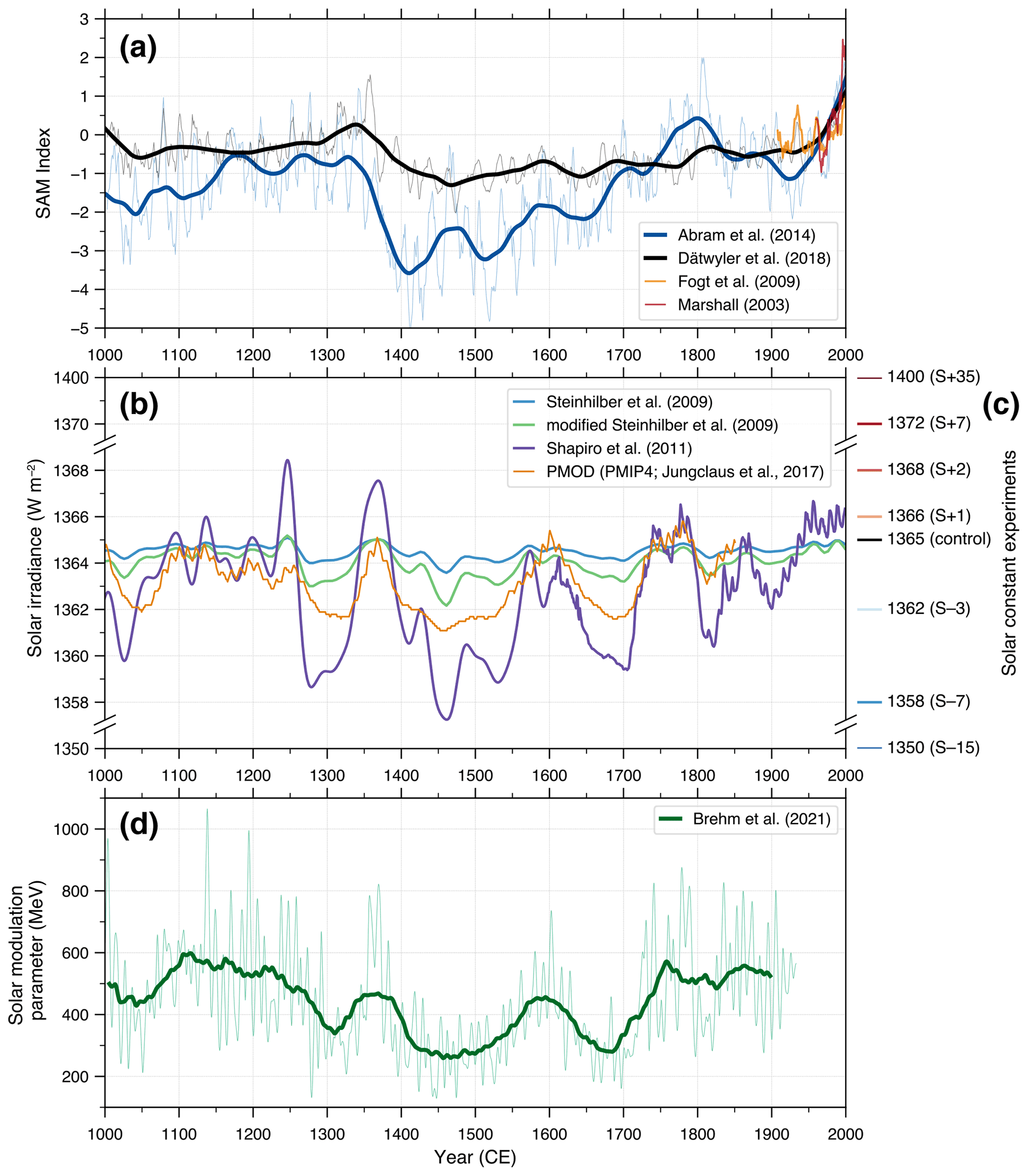
Figure 1Reconstructed SAM and solar variability over the last millennium. (a) Observation-based mean annual SAM indices (normalised units) of Marshall (2003) (red) and Fogt et al. (2009) (orange) and the reconstructed SAM index of Abram et al. (2014) (A14, blue) and Dätwyler et al. (2018) (D18, black; see Sect. 2.1 for an explanation of the difference in magnitude between the SAM reconstructions). The reconstructions are plotted as a 7-year moving average for the annual SAM index (thin lines) with a 70-year LOESS filter (thick lines), while 7-year moving averages are shown for the observational data. (b) Total solar irradiance reconstructions for the last millennium, including Steinhilber et al. (2009) (blue) and a modified version of Steinhilber et al. (2009) (green), where the amplitude of the variations relative to the long-term mean has been increased by a factor of 2 and Shapiro et al. (2011) (purple). For comparison with the current high-amplitude scenario, we also include the PMOD reconstruction from PMIP4 (Jungclaus et al., 2017) (orange). Note that PMOD has been normalised to 1365 W m−2 to be comparable to the other solar reconstructions presented here. (c) Solar irradiance values for our solar constant experiments, with the experiment name provided in parentheses. (d) Solar modulation parameter reconstruction for the last millennium based on radiocarbon from annually resolved and dated tree rings (Brehm et al., 2021) and shown as monthly resolution (thin lines) and a 70-year moving average (thick lines).
Climate simulations of the SAM response to rising atmospheric greenhouse gas levels and stratospheric ozone depletion over the last century compare reasonably well to observations and proxy data (Miller et al., 2006; Raphael and Holland, 2006; Swart and Fyfe, 2012; Gillett and Fyfe, 2013; Zheng et al., 2013). However, further back in time, models are unable to reproduce the structure or magnitude of pre-industrial SAM trends that are reconstructed from proxies (Abram et al., 2014). This could be due to errors in the reconstructions or a systematic issue in the way the SAM is forced or represented in current climate models (Abram et al., 2014; Gillett and Fyfe, 2013). Visually, the temporal evolution of the reconstructed SAM over the last millennium resembles some of the characteristics of long-term changes in solar irradiance over this time (Fig. 1a–c).
Variations in the solar constant (i.e. the rate at which energy reaches the Earth's surface from the sun) have previously been suggested as an important driver of the SAM on observational timescales (Kuroda et al., 2007; Kuroda and Kodera, 2005; Kuroda and Shibata, 2006; Roscoe and Haigh, 2007; Lu et al., 2011). The solar constant varies naturally in an 11-year solar cycle, and recent work using changes in radiocarbon (14C) from annually resolved and accurately dated tree rings confirms that the 11-year cycle was present throughout the last millennium (Brehm et al., 2021) (Fig. 1d). Other proxies (e.g. cosmogenic isotopes such as beryllium-10, 10Be) also indicate that longer-term trends in solar forcing occur on century and millennial scales (Steinhilber et al., 2009; Gray et al., 2010). During the last millennium, solar modulation reached a minimum during the Spörer (1388–1558 CE) and Maunder (1621–1718 CE) grand solar minima events.
Precise observations of solar irradiance (via satellites) are only available from 1978 onward, and thus reconstructions of past changes in the magnitude of solar irradiance rely directly or indirectly on the relationship between proxies (e.g. 14C, 10Be, sunspot properties) and solar irradiance, combined with processing and calibration. Consequently, there are different published magnitudes for solar irradiance changes during the last millennium (Fig. 1b); however, the reconstructions are broadly similar in their temporal history of changes in solar forcing. Many solar reconstructions (including those outlined in the Paleoclimate Modelling Intercomparison Project, phase 3 (PMIP3) v1.0 protocol; Schmidt et al., 2011) have a ∼1.5 W m−2 peak-to-peak variation in total solar irradiance (TSI) between the present day and the Maunder Minimum period (Judge et al., 2012). A high-amplitude (∼6 W m−2 peak-to-peak variation) solar reconstruction (Shapiro et al., 2011) was also included as part of the PMIP3 v1.1 protocol (Schmidt et al., 2012), but it has been argued that this reconstruction overestimates the changes in TSI by a factor of 2 due to the model used in their methodology (Judge et al., 2012). Phase 4 of the Paleoclimate Modelling Intercomparison Project (PMIP4) provides an alternative solar irradiance scenario (“PMOD”) derived using a similar approach to Shapiro et al. (2011) and Judge et al. (2012), with a Maunder Minimum to present amplitude of ∼3.4 W m−2 (Jungclaus et al., 2017), which is almost half the amplitude of Shapiro et al. (2011) but still considerably larger than alternative solar reconstructions for the last millennium. This PMOD reconstruction is currently considered to be the “upper limit” on the magnitude of solar irradiance change (Jungclaus et al., 2017). Existing last millennium climate simulations have almost exclusively been run using the low-amplitude solar-forcing scenarios (e.g. Steinhilber et al., 2009) and in model set-ups that do not accommodate solar-relevant atmospheric chemistry or wavelength specification. This raises the possibility that the effects of solar forcing may not have been adequately included in last millennium simulations, potentially accounting for data–model SAM discrepancies.
Here we explore the sensitivity of the SAM to variations in solar forcing in an attempt to understand if variations in solar irradiance may have affected SAM variability over the last millennium (Fig. 1). We explore simulations with constant solar-forcing values that correspond to the range of total solar irradiance values from the high-amplitude solar reconstruction of Shapiro et al. (2011) and additional extreme solar-forcing values. In addition, we investigate transient simulations for the last millennium using intermediate- and high-amplitude solar-forcing scenarios that complement existing low-amplitude transient solar-forcing experiments. Our findings demonstrate that the mean state of the SAM can be significantly altered by changes in solar irradiance and that transient solar forcing of a magnitude equivalent to high-amplitude scenarios for the last millennium are sufficient for a significant solar effect on the SAM to become evident despite the large magnitude of internal SAM variability. Last millennium simulations using high-amplitude solar forcing show an improved agreement with proxy-based SAM reconstructions, suggesting that the effects of solar forcing may not be adequately represented in current last millennium climate model simulations.
2.1 Reconstructions
The last millennium reconstructions that we use in this study are for the annual mean SAM index. These are based on (i) a multiproxy network spanning Antarctica and South America where the temperature anomalies caused by SAM variations are strong (Abram et al., 2014) and (ii) an extensive network of proxies from across the Southern Hemisphere using a long calibration period and a correlation plus stationarity criterion for proxy selection (Dätwyler et al., 2018). Hereafter, these SAM reconstructions are referred to as A14 (Abram et al., 2014) and D18 (Dätwyler et al., 2018). The A14 and D18 reconstructions share similar features in their long-term trends (Fig. 1a) despite potential regional biases in the proxy networks used for the reconstructions and uncertainty related to non-stationary proxy–SAM relationships (Huiskamp and McGregor, 2021; Hessl et al., 2017). Both reconstructions indicate that the most negative phase of SAM conditions occurred during the 1400s prior to a progressive, multi-century positive trend in the SAM since the 1400s, including the rapid 20th century increase in the SAM. Both reconstructions also record strong interannual to centennial variability on top of these long-term trends, with this characteristic particularly evident in the A14 reconstruction.
The A14 and D18 reconstructions were both developed using the instrumental SAM index as a calibration target (i.e. Marshall, 2003, and Fogt et al., 2009, respectively); however, the A14 reconstruction displays a larger magnitude of variability (Fig. 1a). This difference in magnitude is due to differences in the way the annual SAM index can be calculated from instrumental data (Fig. 2). For example, the instrumental SAM index (Marshall, 2003; http://www.nerc-bas.ac.uk/icd/gjma/sam.html, last access: 14 April 2021) is publicly available in both monthly and annual resolutions. Here, the annual-resolution SAM index is calculated directly using the differences of annual means of mean sea level pressure (MSLP) data at 40 and 65∘ S. Alternatively, the monthly resolution SAM data (calculated from differences of monthly means of MSLP data at 40 and 65∘ S) can be used to then calculate annual averages of the SAM. The two approaches result in similar trends and interannual variability of the SAM; however, the magnitude of the directly calculated annual SAM index is 2.7 times larger than the annual mean SAM derived from the monthly SAM index (Fig. 2).
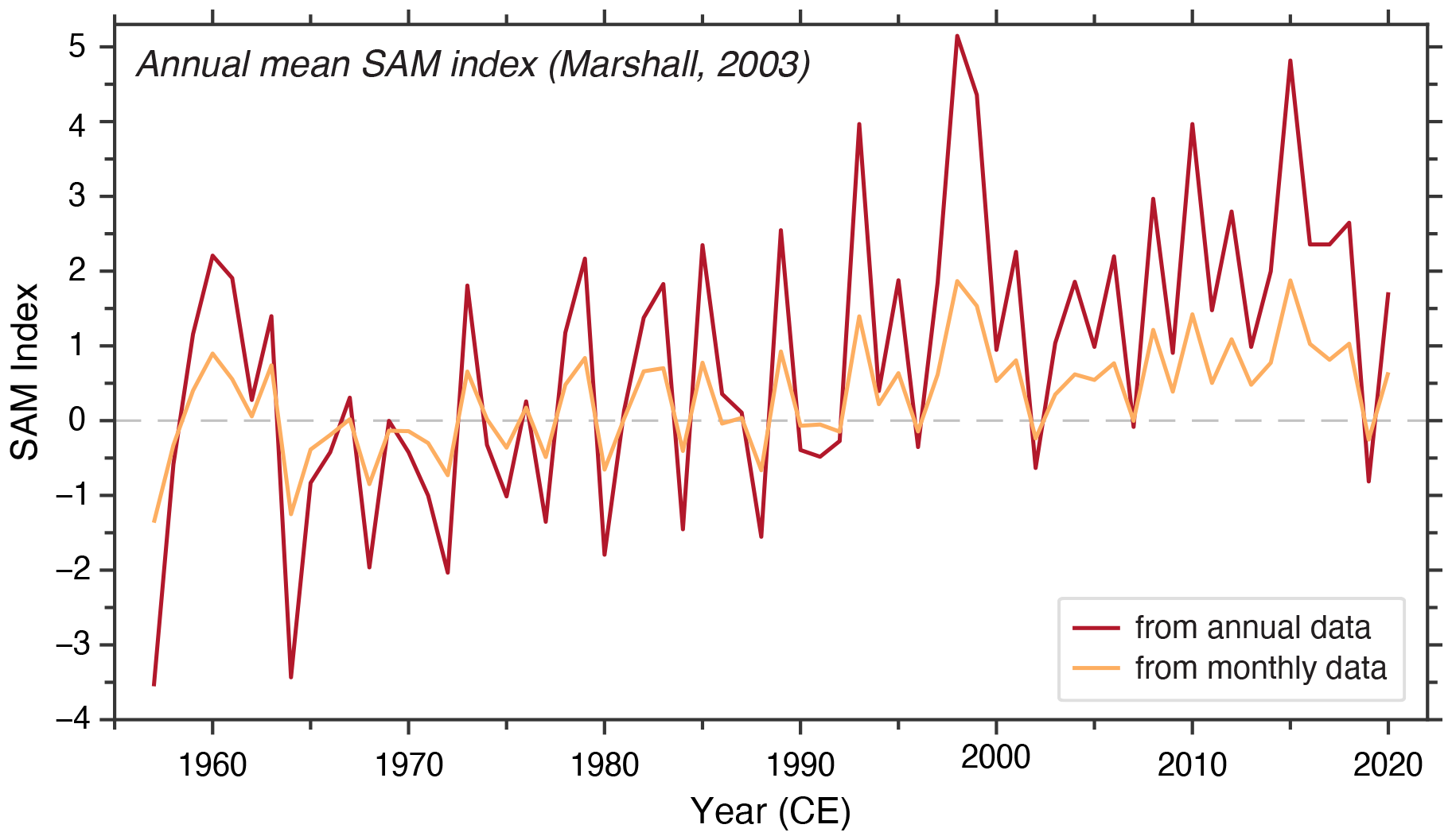
Figure 2Difference in the observed annual SAM index when calculated using monthly MSLP anomalies (i.e. using normalised monthly MSLP anomalies at 40 and 65∘ S and then averaging this monthly SAM index into an annual time series; orange line) and annual MSLP (i.e. normalised MSLP anomalies at 40 and 65∘ S; red line). Data are from Marshall (2003), and the updated index is publicly available (http://www.nerc-bas.ac.uk/icd/gjma/sam.html, last access: 14 April 2021).
The A14 and D18 SAM reconstructions both use an annual SAM index as their calibration target, but A14 used a calibration annual mean SAM index calculated from annual data (i.e. red line in Fig. 2), while D18 used a calibration annual mean SAM index calculated from monthly data (e.g. orange line in Fig. 2). Consequently, while the two reconstructions produce similar patterns and trends of annual SAM variability during the last millennium, they have markedly different magnitudes of change due to differences in the instrumental calibration data used (Fig. 3a). To confirm this, we recalculate the A14 reconstruction using the alternate calibration target (i.e. calibrated to the annual SAM index derived from monthly SAM data, as in the D18 reconstruction). This rescaled reconstruction (referred to hereafter as A14-rescaled) has interannual to centennial variability and trends in the last millennium that are of similar magnitude as the D18 reconstruction (Fig. 3b), confirming that the source of apparent discrepancy between the A14 and D18 reconstructions is primarily due to the different instrumental targets used to calibrate the reconstructions.
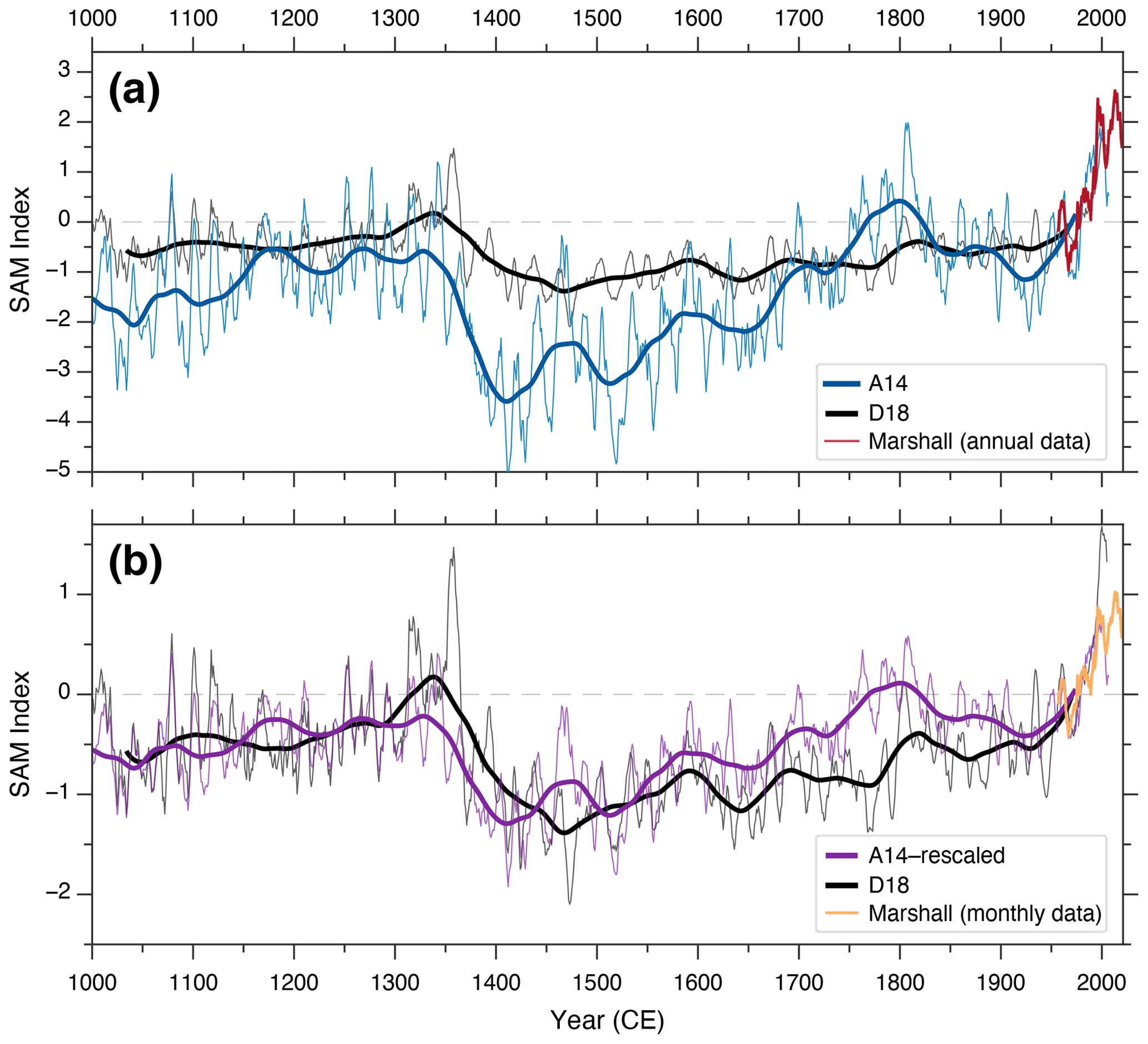
Figure 3The effect of calibration target on scaling of last millennium SAM reconstructions. (a) Observation-based annual SAM index (Marshall, 2003) calculated using annual MSLP anomalies (red line; shown as 7-year moving average), which forms the calibration target for the A14 SAM reconstruction (blue line; shown as a 7-year moving average and 70-year loess filter by thin and thick lines, respectively). (b) Observation-based annual SAM index (Marshall, 2003) calculated using monthly MSLP anomalies (orange line; shown as 7-year moving average) and the result that this alternate calibration target has on the scaling of A14 SAM reconstruction (purple line; shown as a 7-year moving average and 70-year loess filter by thin and thick lines, respectively). For comparison, the D18 SAM reconstruction is shown in black (7-year moving average and 70-year loess filter by thin and thick lines, respectively) in both panels (a) and (b) and is based on a monthly derived annual SAM index as the calibration target.
In this study, we use the A14, D18, and A14-rescaled SAM reconstructions as indicators of temporal changes in the mean state of SAM during the last millennium. These are used in data–model comparisons to determine if different solar-forced model simulations are able to reproduce characteristics of reconstructed SAM changes during the last millennium.
2.2 Model simulations
The model simulations in this study were performed using the Commonwealth Scientific and Industrial Research Organisation Mark 3L (CSIRO Mk3L) coupled climate system model, version 1.2 (Phipps et al., 2011, 2012, 2013). CSIRO Mk3L is a fully coupled general circulation model that includes components describing the atmosphere, ocean, sea ice, and land surface. The horizontal resolution of the atmosphere, sea ice, and land surface models is in the longitudinal and latitudinal dimensions, respectively, with 18 vertical levels. The horizontal resolution of the ocean model is , with 21 vertical levels. CSIRO Mk3L was used within this study as it is computationally efficient, allowing for many multi-century- to millennia-scale experiments to be performed.
We investigate how the SAM changes in a series of “solar constant” experiments and transient experiments. Specifically, we perform the following experiments.
- a.
Seven solar constant experiments are performed, where the solar constant (i.e. TSI, with no wavelength dependence) was changed to capture the range of proxy-based realistic solar values in the Shapiro reconstruction (−7, −3, +1, and +3 W m−2 anomalies relative to a 1365 W m−2 control) and unrealistic extreme solar forcings (e.g. −15, +7, and +35 W m−2 anomalies) to test the response of the model (Fig. 1c). These experiments use pre-industrial CO2 (280 ppm), and we run each experiment to equilibrium. In our analysis of the model output we primarily focus on the transient response of the SAM to the changed solar constant within the first 200 years of each run (Fig. 4), where the climate has not yet equilibrated to the new solar forcing. These experiments are referred to using their solar constant anomaly value (e.g. S−7, S+3, etc.)
- b.
Three-member ensembles of transient experiments using three solar-forcing scenarios for the last millennium are performed. These transient experiments were initialised from the control used in Phipps et al. (2013) (refer to Phipps et al., 2013, for further details), and all examples include orbital, greenhouse gas, and solar forcings. The first ensemble is the orbital–greenhouse gases–solar (OGS) ensemble first published in Phipps et al. (2013), which uses the Steinhilber et al. (2009) solar forcing. We build upon this OGS ensemble by performing additional experiments with modified solar forcing (Fig. 1b). The second ensemble of transient experiments uses an amplified Steinhilber et al. (2009) forcing, where the magnitude of the transient solar-forcing anomaly relative to the long-term mean is doubled (hereafter referred to as OGS-x2). The third ensemble of transient experiments uses the Shapiro et al. (2011) high-amplitude solar forcing that was included as a last millennium forcing option in the PMIP3 v1.1 protocol (Schmidt et al., 2012) and is hereafter referred to as OGS-Shapiro. The CSIRO Mk3L model does not include interactive chemistry, and we do not prescribe ozone variations scaled to the solar forcing in our experiments in an attempt to replicate the response of atmospheric chemistry during the last millennium. Each experiment was run for 1–2000 CE. Here, we focus our analysis on 850–1900 CE to avoid the influence of strong anthropogenic greenhouse gas forcings after 1900.
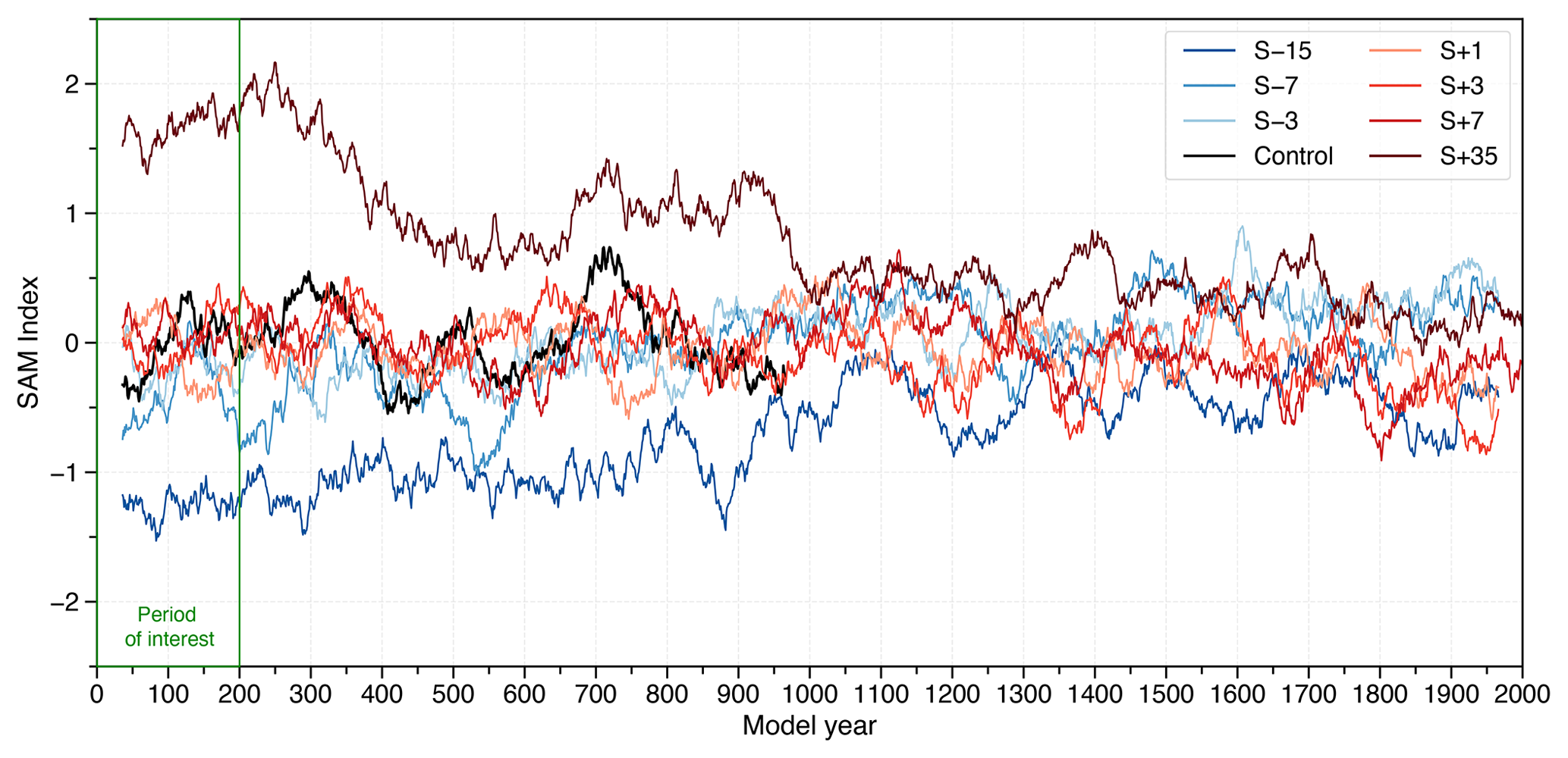
Figure 4The 70-year moving average for the annual SAM index for each solar constant simulation. The period of interest in this study (first 200 years) is indicated with a green box.
We supplement our transient experiments with CSIRO Mk3L using previously published simulations based on the HadCM3 model (“Euroclim500”; Schurer et al., 2014). These simulations include one full-forcing ensemble member for 800–2000 CE, three full-forcing ensemble members for 1400–2000 CE, four “weak-solar-only” ensemble members for 1400–2000 CE, and one “solar-Shapiro-only” run for 800–2000 CE using the solar reconstruction from Shapiro et al. (2011). Forcings used in the HadCM3 experiments follow the PMIP3 protocol (Schmidt et al., 2011, 2012); specifically, the solar reconstruction used in the full-forcing and weak solar runs is based on a combination of Steinhilber et al. (2009) (for times prior to 1810) and Wang et al. (2005) (for 1810–2000 CE) (see Schurer et al., 2014, for further details). We note that both our CSIRO Mk3L experiments and these HadCM3 experiments do not have an interactive ozone.
The SAM index was calculated for each model run using the following definition taken from Gong and Wang (1999):
where P* is the normalised annual zonal mean MSLP anomaly in the model relative to climatology. For the solar constant experiments, we use the solar constant (1365 W m−2) control run as our climatology. This allows us to assess the effect of modifying the solar constant anomaly on the SAM mean state in the other solar constant experiment relative to the 1365 W m−2 control. We use a Welch's t test and a Kolmogorov–Smirnov test to assess the difference between our solar constant experiments and the control run. In the transient experiments we use the 1900–1999 CE period as our climatology to assess pre-industrial changes in the SAM mean state over the last millennium, and use a Wilcoxon rank-sum test, linear least-squares regression, and bootstrapping approach to compare our transient experiments with its radiative forcing and the SAM reconstructions.
3.1 Solar constant experiments
The solar constant experiments demonstrate how changes in the intensity of solar forcing influence the SAM mean and extreme states (Figs. 5, 6). The distribution of the mean annual SAM index is significantly different from the control in the S−15, S−7, and S+35 experiments (based on Welch's t test, P<0.05, see Fig. 5a). In particular, changing the solar constant results in a mean shift in the SAM but no significant difference in the magnitude of SAM variability about this mean shift (using a Kolmogorov–Smirnov test, P>0.05) (Fig. 5a). This mean shift in the SAM results in a change in the number of extreme events (outside ±2σ of the control run), whereby a reduced solar forcing (i.e. S−15, S−7, and S−3) results in an increase in extreme negative SAM events and decrease in extreme positive SAM events and vice versa for the increased solar-forcing experiments (Fig. 5b).
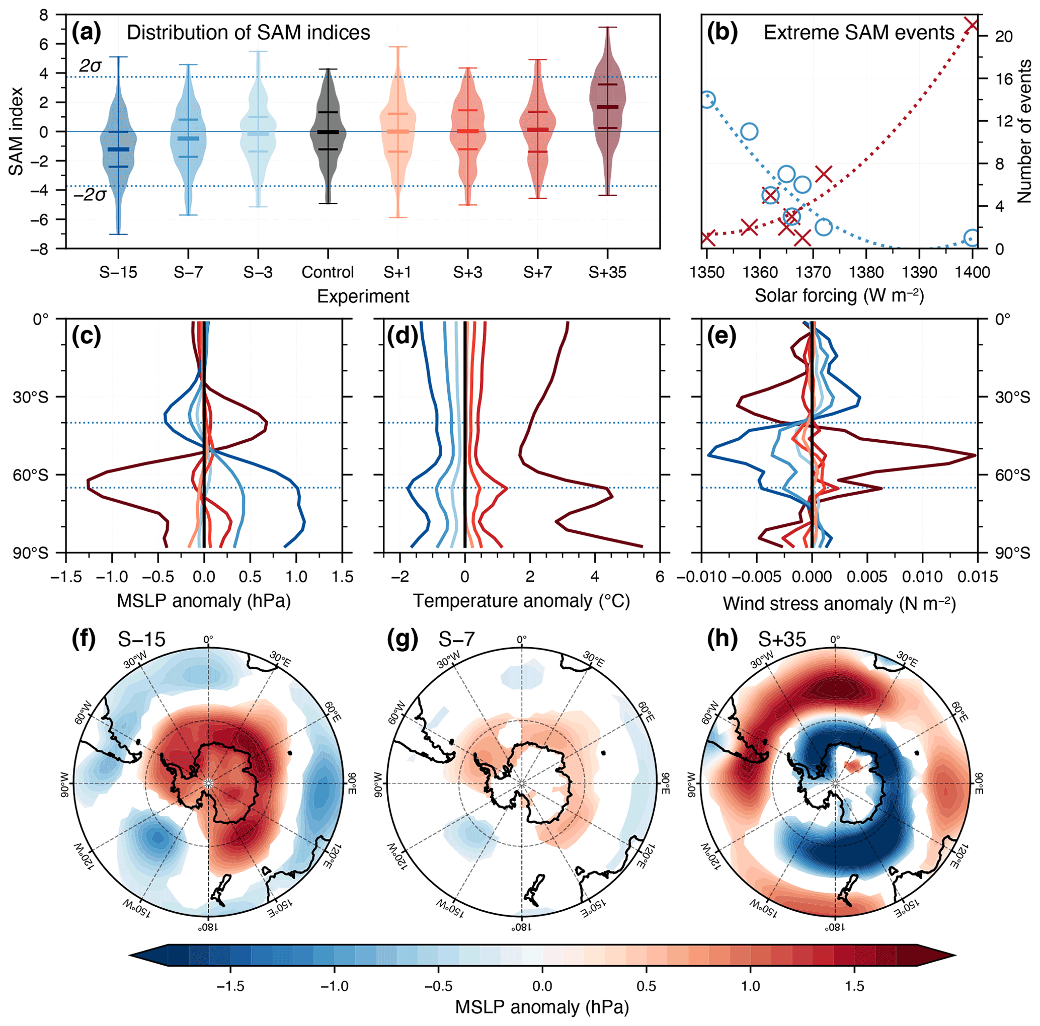
Figure 5SAM index and events for the first 200 years of fixed solar-forced model runs. (a) Violin plots of the distribution of mean annual SAM index calculated for each solar constant run. Coloured horizontal lines refer to the 25th percentile, mean, and 75th percentile. (b) Number of extreme SAM events (outside ±2σ of the control run) in 200 years, with a second-order line of best fit for positive and negative events. Blue circles refer to extreme negative SAM events, and red crosses refer to extreme positive SAM events. (c–e) Zonal mean anomalies for the first 200 years of the experiments for (c) mean sea level pressure, (d) surface air temperature, and (e) surface zonal wind stress (positive values indicate westerly anomalies), where the anomaly is relative to the control run. Colours for each experiment correspond to those used in panel (a). Dashed lines at 40 and 65∘ S are the latitudes used to calculate the SAM index. (f–h) MSLP anomalies relative to the control for the first 200 years in the (f) S−15, (g) S−7, and (h) S+35 experiments. Regions shown are significantly different to the control run (based on Welch's t test, P<0.05); areas where P≥0.05 have been masked out.
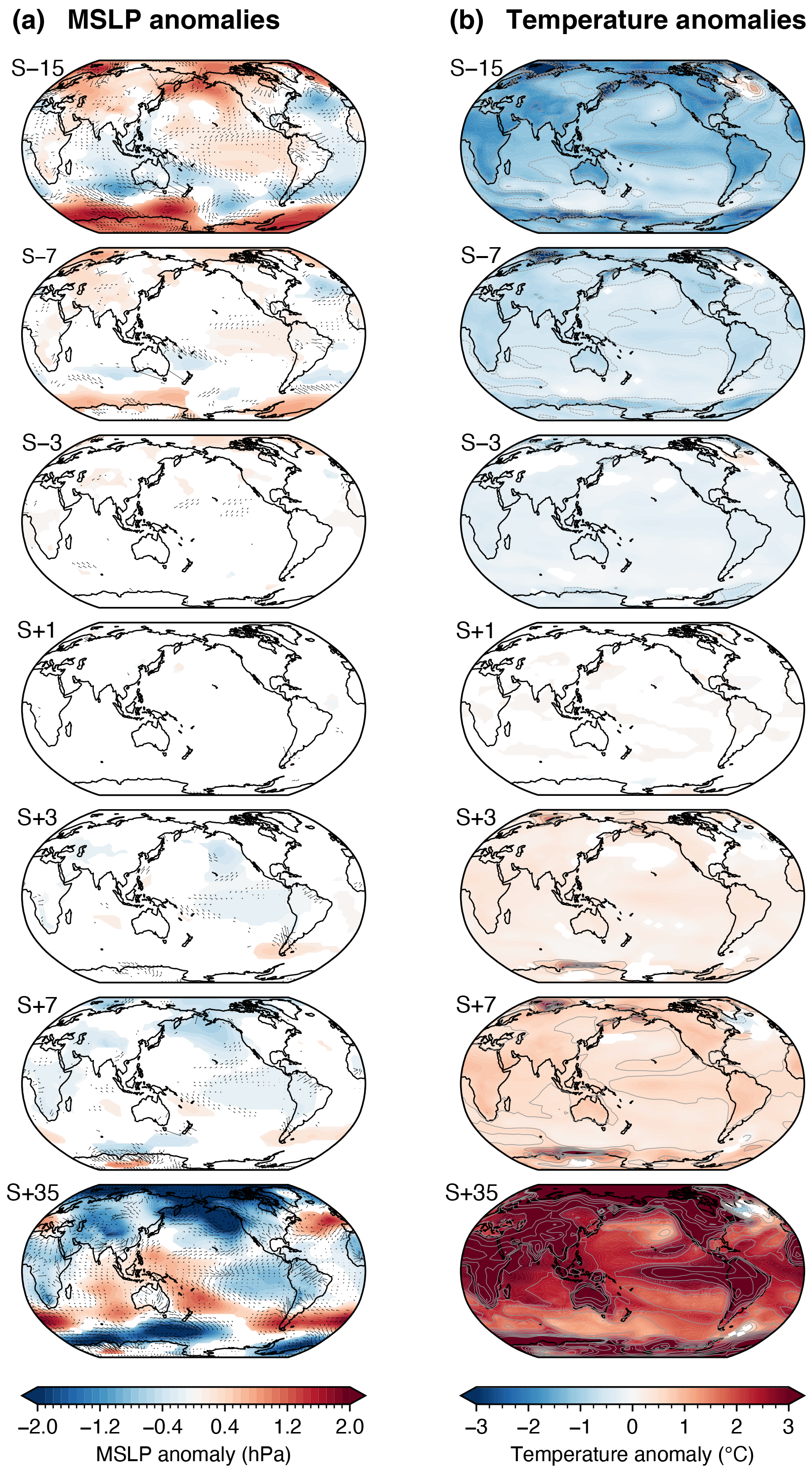
Figure 6Surface anomalies (relative to the control run) for the first 200 years of the different solar constant experiments. (a) MSLP anomaly (shaded) and surface wind anomalies (vectors). (b) Surface temperature anomaly (shaded), with temperature contours additionally shown at 0.5 ∘C increments (to assist in interpreting S+35). Regions that are significantly different (based on a Welch's t test, P<0.05) are shown, while areas where P≥0.05 have been masked out.
The spatial patterns of anomalies in the solar constant experiments demonstrate the consistent influences that changes in solar intensity have on the SAM and Southern Hemisphere climate (Fig. 5c–h). Negative solar-forcing anomalies result in a decrease in MSLP over the Southern Hemisphere mid-latitudes and an increase in MSLP over the Antarctic, and thus a reduced meridional pressure gradient between these zones (Fig. 5c, f–g). This is associated with an enhancement of the surface temperature gradient between the mid-latitudes and Antarctica (Fig. 5d; i.e. Antarctica cools more than the mid-latitudes) and decreased westerly wind anomalies in the Southern Ocean jet (Fig. 5e), leading to a mean negative shift in the SAM index and an increase in the number of extreme negative SAM events relative to extreme positive events. The opposite is also true with positive solar forcing, which leads to increased MSLP over the mid-latitudes and decreased MSLP over Antarctica and consequently strengthens the meridional pressure gradient and the westerly wind jet. This results in a more positive mean SAM, with an increase in the frequency of extreme positive SAM events. We note that there is an asymmetry in the effect of changing the solar constant, with a larger response seen in the negative solar constant experiments (i.e. S−3, S−7) than the positive solar constant anomalies (i.e. S+3, S+7) (Fig. 5a–e). The solar constant experiments also show that the magnitude of MSLP change over the Antarctic (65∘ S) is larger than over the mid-latitudes (40∘ S) in response to changes in solar forcing (Fig. 5c).
3.2 Transient experiments for the last millennium
The transient simulations build upon our findings from the solar constant experiments by modelling the time evolution of the SAM index during the last millennium based on different amplitudes of transient solar forcing (Figs. 7, 8). The simulations also include transient orbital and greenhouse gas forcing, and thus we express the results using radiative forcing (i.e. the combined radiative forcing of orbital, greenhouse gas, and solar instead of solar irradiance only) and focus on pre-industrial times (i.e. prior to 1900). The ensemble mean SAM index from the low solar amplitude OGS experiments (Phipps et al., 2013) is not significantly correlated with the radiative forcing. This indicates that the low-amplitude solar forcing in these simulations is not large enough to modulate the mean SAM state in a way that is detectable beyond the magnitude of unforced internal SAM variability. We additionally find that the OGS-ensemble mean is largely within the range of unforced internal SAM variability during the last millennium (Fig. 7c), where our internal variability is represented using the ±2σ range from the orbital-only (O) simulations (Fig. 7a). We further assess this relationship by applying a bootstrapping approach to randomly reorder the OGS ensemble mean SAM (N=10 000) and find that the OGS SAM index is not significantly correlated with its radiative forcing any more than could be explained by a random distribution of the model data. However, the ensemble mean SAM index from the intermediate solar amplitude OGS-x2 experiments is positively correlated with radiative forcing for pre-industrial times (r=0.43, P<0.05, effective sample size Neff=15.8; based on 70-year moving averages stepped by 35 years, with effective sample size taking into account lag-1 autocorrelation of the time series; Fig. 8a–b). The OGS-x2 ensemble mean also exceeds the range of internal variability during some intervals of the last millennium (particularly during the 15th century) where the SAM is more negative than can be explained by internal variability alone (Fig. 7d). However, for individual ensemble members with intermediate-amplitude solar forcing, we cannot reject the null hypothesis that there is no correlation. Using a bootstrapping approach (N=10 000) to our OGS-x2 ensemble mean SAM index further finds a significant correlation with its radiative forcing (P<0.05) relative to a random distribution of the model data.
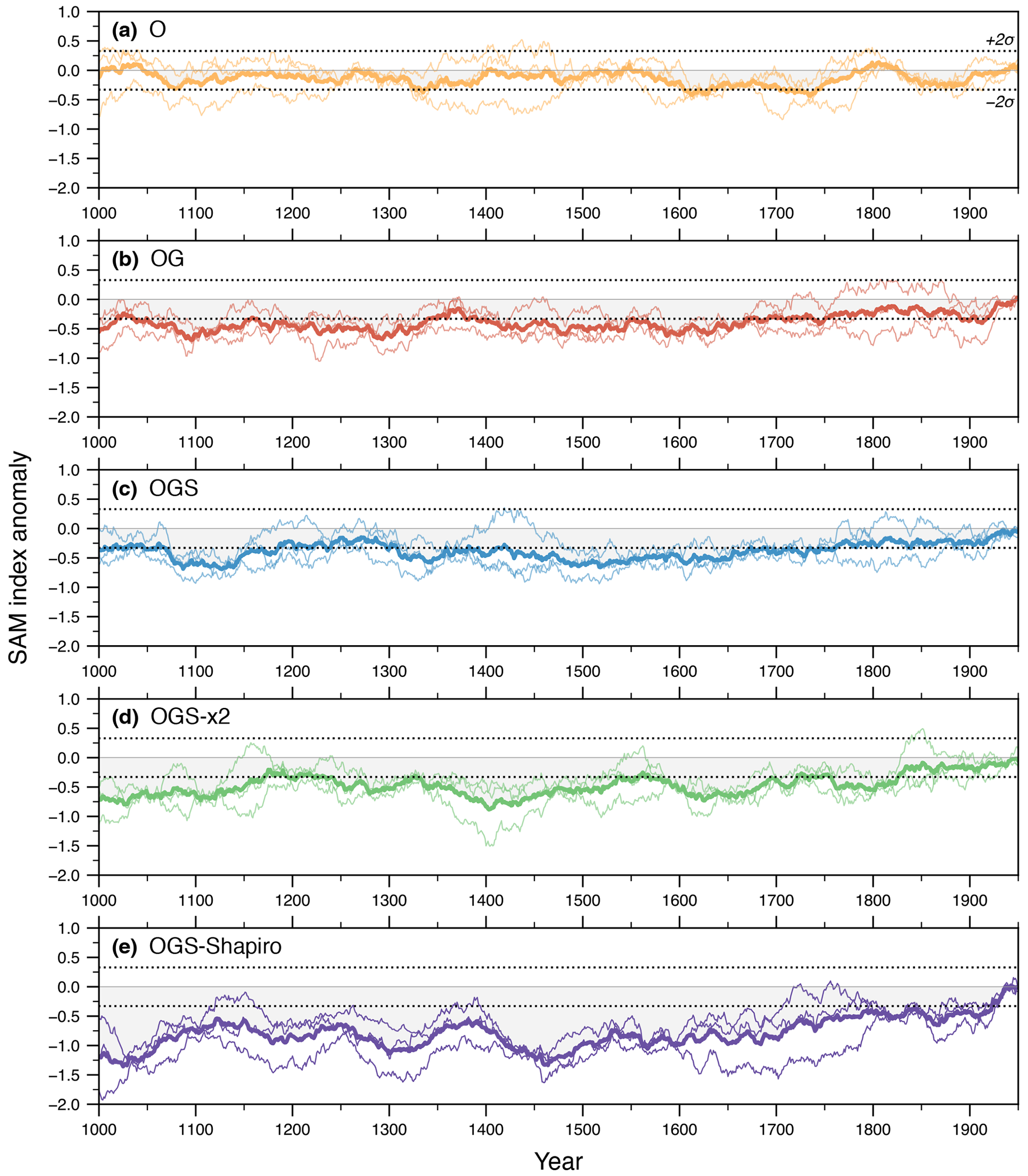
Figure 7SAM index anomaly based on the different Mk3L simulations. SAM index anomaly is calculated relative to 1900–1999 CE mean and shown as 70-year moving averages. (a) Orbital-only (O) simulation; (b) orbital and greenhouse gases (OG) simulation; (c) orbital, greenhouse gases, and low-amplitude solar-forcing (OGS) simulation; (d) orbital, greenhouse gases, and the intermediate-amplitude solar-forcing (OGS-x2) simulation; (e) orbital, greenhouse gases, and high-amplitude solar (OGS-Shapiro) simulation. Thick lines refer to the ensemble mean, while thin lines denote the individual ensemble members. Dashed lines on all subplots show the ±2σ range based on the orbital-only (O) simulations, representing internal variability.
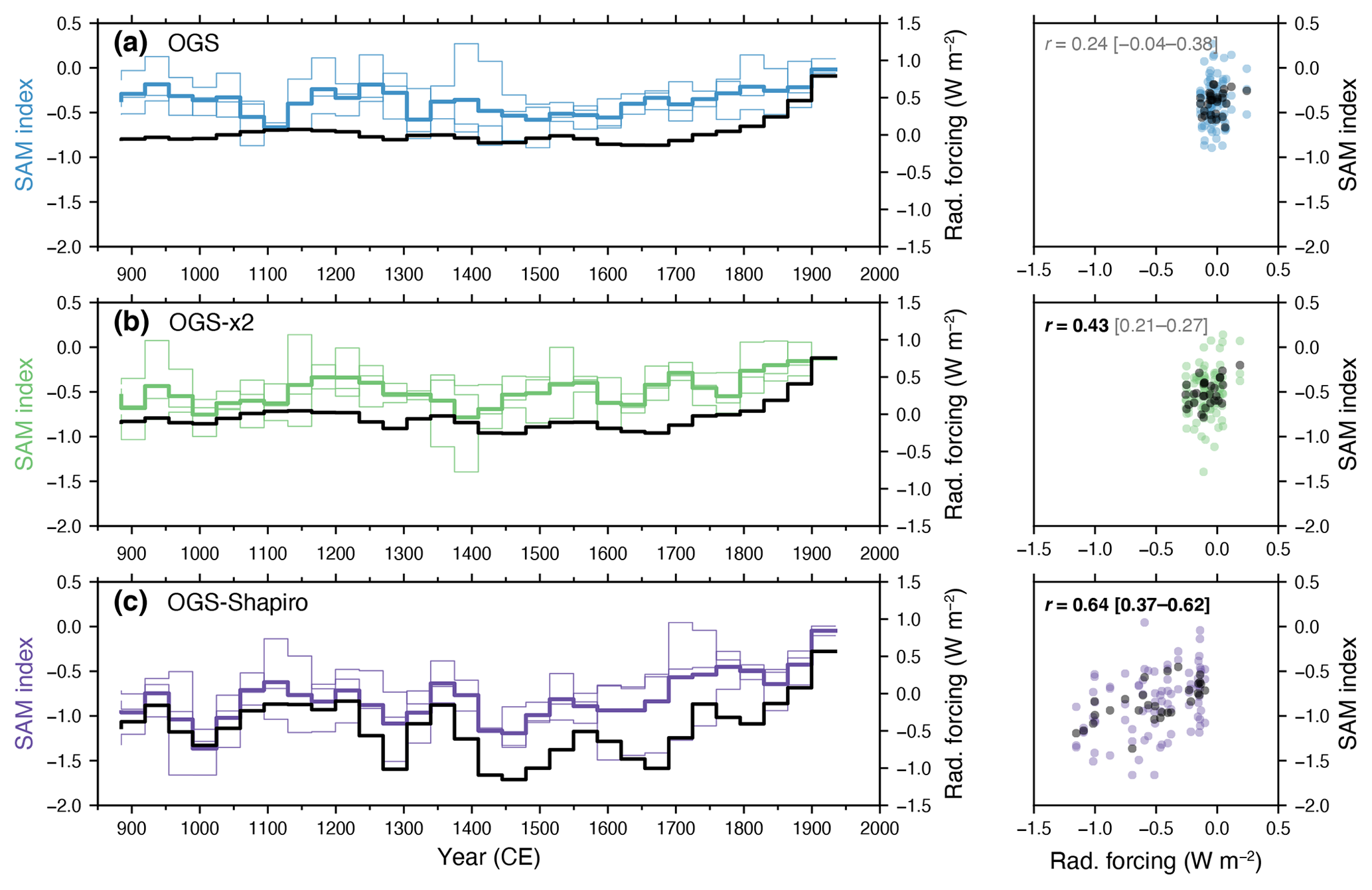
Figure 8SAM index response to different amplitudes of transient solar forcing during the last millennium. Time series (left column) of the SAM index (coloured lines; ensemble mean: thick line; ensemble members: thin lines) and radiative forcing anomalies (black) in the transient experiments with (a) low-, (b) intermediate-, and (c) high-amplitude solar forcing. Time series shown for the SAM index are calculated relative to 1900–1999 climatology, and long-term changes are represented as 70-year moving averages stepped by 35 years. Scatter plots (right column) show the 850–1900 CE correlation between 70-year moving averages stepped by 35 years of the SAM index and radiative forcing anomalies in the ensemble mean (black, first r value) and ensemble members (coloured, r values in square brackets give ranges across ensemble members); r values in bold text are where P<0.05, while r values in grey text are where there is no significant relationship. Correlations are limited to 850–1900 CE to avoid the influence of recent anthropogenic greenhouse gas influences on the radiative forcing–SAM relationship.
In contrast, the SAM index for the high-amplitude OGS-Shapiro simulations is significantly correlated with the radiative forcing anomaly (Fig. 8c). The correlation coefficient between radiative forcing and the SAM index in the ensemble mean is 0.64 (P<0.05, Neff=14.4) for pre-industrial times (i.e. 850–1900 CE). The correlation between the OGS-Shapiro ensemble mean SAM index and its radiative forcing remains significant (P<0.05; relative to a random distribution of the model data) when tested against a bootstrapping approach (N=10 000). Each of the individual ensemble members in the high-amplitude solar experiments also displays a significant long-term SAM–radiative forcing relationship over the last millennium, demonstrating a forced signal detectable beyond the large range of internal SAM variability (Fig. 7e).
We explore this relationship further by binning the model results across all of the transient experiments based on the magnitude of radiative forcing (Fig. 9). Increasingly negative radiative forcing anomalies result in an increasingly negative SAM index (Fig. 9a–b). Binning across all ensemble members based on radiative forcing anomalies further illustrates the linear relationship between reduced radiative forcing and a more negative mean SAM (Fig. 9b). The zonal mean MSLP and temperature profiles (Fig. 9c–d) and spatial structure of MSLP anomalies (Fig. 9e–h) are consistent with the anomalies produced in the solar constant experiments (Fig. 5). This suggests a consistent response of mid- to high-latitude Southern Hemisphere climate to changes in solar forcing within the CSIRO Mk3L experiments that is also robust across different experiment designs.

Figure 9SAM index response to different levels of radiative forcing compiled across solar transient experiments. (a) Violin plots of the 70-year rolling mean SAM index between 850 and 1900 CE; lines refer to the 25th percentile, mean, and 75th percentile. (b) Scatter plot of 70-year rolling mean for radiative forcing anomaly and the SAM index where r=0.78 (P<0.05). (c–d) Zonal mean anomalies for (c) mean sea level pressure (MSLP) and (d) temperature, where the anomaly is relative to the climatological (1900–1999 CE) mean. Coloured lines refer to the radiative forcing bins for −1.5 to −1.0 W m−2 (purple), −1.0 to −0.5 W m−2 (blue), −0.5 to 0.0 W m−2 (orange), and 0.0 to 0.5 W m−2 (red). (e–h) MSLP anomalies (relative to the climatological mean based on radiative forcing bins). Regions shown are significantly different to the OGS ensemble mean (based on Welch's t test, P<0.05); areas where P≥0.05 have been masked out. Dashed lines at 40 and 65∘ S are the latitudes used to calculate the SAM index.
Overall, our experiments show that a decrease in solar radiative forcing (in both the constant solar and transient solar-forcing runs) results in a mean negative SAM shift. Reducing solar forcing by 1.5–1.0 W m−2 is roughly equivalent to a ∼7 W m−2 reduction in the solar constant (based on scaling the change in TSI by ; Lean and Rind, 1998). Both the S−7 fixed solar constant experiment and high-amplitude transient radiative forcing of −1.5 to −1.0 W m−2 result in a statistically significant negative anomaly in the SAM that is detectable despite the large magnitude of unforced internal variability of the SAM. These simulation results with the CSIRO Mk3L model suggest that reconstructed negative SAM conditions during the last millennium could have been the result of reduced solar forcing at this time.
Previous work using low-amplitude solar-forcing experiments has not found any significant relationship between solar forcing and reconstructed long-term changes in the annual SAM during the last millennium (Abram et al., 2014; Dätwyler et al., 2018). However, extreme changes in solar forcing in our model experiments that are comparable with high-amplitude estimates of solar irradiance anomalies during the last millennium (Shapiro et al., 2011) are able to produce a significant change in the mean SAM index, where a −7 W m−2 change in solar irradiance (or a roughly −1.23 W m−2 change in radiative forcing) results in a significant negative shift in the mean SAM index. To further explore whether solar forcing may help to explain reconstructed trends in the SAM during the last millennium, we compare our model results with proxy-based SAM reconstructions (see Sect. 2.1).
To test the significance of changes in the SAM during the last millennium, we use each of the SAM reconstructions to assess whether 70-year sliding windows of the annual SAM reconstructions are significantly (P<0.05; Wilcoxon rank-sum test) more negative than a 70-year reference window of the reconstruction between 1831 and 1900 CE. This reference interval was chosen as it is prior to strong positive SAM trends caused by anthropogenic forcing during the 20th century and is longer than the standard 50-year pre-industrial period so as to improve the robustness of the distribution testing. These tests show that across all three reconstructions the SAM index was significantly more negative between approximately 1390 and 1715 CE compared with the 1831–1900 CE reference interval (Fig. 10). The A14 and A14-rescaled reconstructions also indicate significant negative SAM distributions prior to around 1140 CE (Fig. 10).
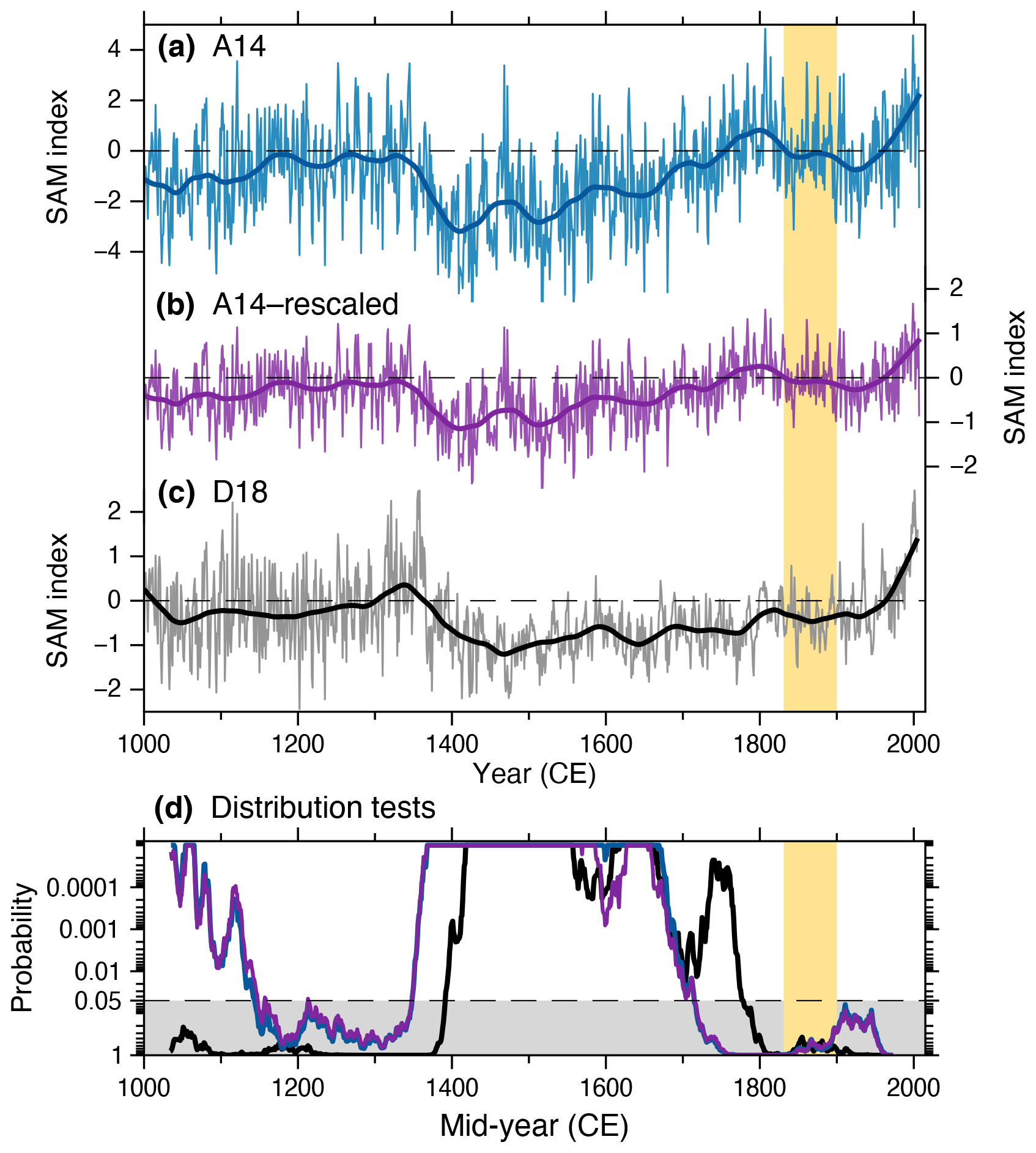
Figure 10Last millennium SAM reconstructions (a–c) and the significance of negative shifts in 70-year distributions through time relative to a 70-year pre-industrial reference period (1831–1900) (d). Annual mean SAM reconstructions (thin curves) and 70-year loess filters (thick curves) for (a) the A14 SAM reconstruction (blue), (b) the A14-rescaled SAM reconstruction (purple; see Fig. 3), and (c) the D18 SAM reconstruction. SAM reconstructions shown relative to 1900–1999 CE climatology (dashed horizontal lines). (d) Distribution tests using a Wilcoxon rank-sum test of moving 70-year windows of each SAM reconstruction, shown in panels (a)–(c), relative to its 70-year pre-industrial reference period (1831–1900 CE; yellow vertical shading). Time series show the probability for the distribution of sliding test windows being more negative than the distribution in the reference interval; values of P<0.05 are shown with a white background, while values of P≥0.05 are shown with a grey background. All three reconstructions show a significant (P<0.05) negative shift in the SAM index compared with the 1831–1900 reference interval during the period from approximately 1390 to 1715 CE. Both versions of the A14 SAM reconstruction also have a significant negative SAM shift prior to around 1140 CE.
Carrying out the same distribution tests on the CSIRO Mk3L transient simulations (Fig. 11) shows that there are no significant negative shifts of the SAM index during the last millennium in the OGS ensemble mean with low-amplitude solar forcing. By comparison, the OGS-Shapiro ensemble mean shows a strong and sustained negative SAM shift that peaked at approximately 1460 CE. This is in good agreement with the interval where all SAM reconstructions also display a significant negative shift in the SAM. The OGS-Shapiro ensemble mean also shows earlier intervals where the SAM index is significantly more negative than the 1831–1900 CE reference interval. Exact matches in the start and end times of significant negative shifts caused by solar forcing in the SAM simulations and reconstructions are not expected due to the additional effect of large unforced internal variability in the SAM (i.e. as seen in differences between ensemble members runs with the same solar forcing). However, we do find that the maximum significance in negative SAM distribution shifts in the OGS-Shapiro ensemble mean is around 1460 CE (Fig. 11d), which matches the timing of maximum significant shifts in all of the last millennium SAM reconstructions (Fig. 10d; approximately 1415–1560 CE). We also find a strongly significant negative shift in the simulated SAM index peaking at around 1025 CE (Fig. 11d), which coincides with the reconstructed significant shift in the A14 and A14-rescaled reconstructions prior to 1140 CE (Fig. 10).

Figure 11SAM index in the CSIRO Mk3L transient last millennium simulations (a–c) and the significance of negative shifts in 70-year windows of annual SAM distributions through time relative to a 70-year pre-industrial reference period (1831–1900 CE) (d). The 70-year loess filter of the SAM index of (a) the OGS simulations, (b) OGS-x2 simulations, and (c) OGS-Shapiro simulations (as in Fig. 8). The ensemble mean is shown as a thick line, and individual ensemble members are shown as thin lines. SAM indices are shown relative to their 1900–1999 CE climatology (dashed horizontal lines). (d) Distribution tests on ensemble means using a Wilcoxon rank-sum test of sliding 70-year windows relative to the pre-industrial reference period (1831–1900 CE; vertical yellow shading), where colours match the SAM simulations shown in panels (a)–(c). Time series show the probability for the distribution of sliding test windows being more negative than the distribution in the reference interval. Values of P<0.05 are shown with a white background, while values of P≥0.05 are shown with a grey background.
Direct correlation of the reconstructions and transient simulations further shows that the A14 proxy-based SAM reconstruction shares significant (P<0.05) variance during the pre-industrial last millennium (1000–1900 CE) with the ensemble mean SAM index of the transient solar scenario simulations run with CSIRO Mk3L (Fig. 12a). The increasing strength of the correlations with increasing magnitude of solar forcing indicates improved coherence between the multi-decadal variability and long-term trends of the reconstructed and modelled SAM when strong solar forcing is used over the last millennium. There are differences in the shorter-term details of the modelled and reconstructed SAM indices, such as the timing during the 1400s when the most negative SAM conditions are reached. However, these differences are of a comparable magnitude to the internal variability between ensemble members of the same experiment (Fig. 8) and thus may simply represent differences between realisations (including the reconstructed single real-world realisation) in unforced variability of the SAM on top of the solar-forced variability and trends.
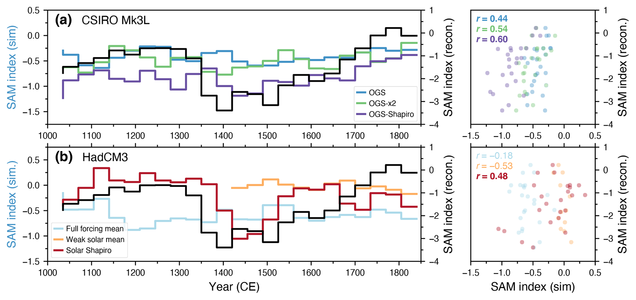
Figure 12Comparison of simulated SAM index and the A14 SAM reconstruction between 1000 and 1900 CE. Time series (left column) of the SAM index (70-year moving averages stepped by 35 years, calculated relative to 1900–1999 CE historical mean) from ensemble means of transient simulations and SAM reconstructions (black line; A14) (a) for transient experiments from CSIRO Mk3L using low- (blue, OGS), intermediate- (green, OGSx2), and high-amplitude (purple, OGS-Shapiro) solar forcing (b) for simulations from HadCM3 (Schurer et al., 2014), including the full-forcing (blue), weak-solar (orange), and strong-solar (“solar Shapiro” runs using Shapiro et al., 2011; red) simulations. Note that there is only a single member for the strong-solar scenario and that the solar-forcing simulations from HadCM3 do not include greenhouse gases (whereas the full forcing simulation does). This results in the last millennium SAM index from the full-forcing simulation having a lower mean than the solar-forcing-only experiments when calculated relative to the 1900–1999 CE historical mean. Scatter plots (right column) show the correlation between the simulated ensemble mean and reconstructed SAM indices, as 70-year moving averages stepped by 35 years, and r values between the simulated and reconstructed SAM index are shown in bold text where P<0.05.
We further explore the robustness of the correlation between the simulated SAM and the A14 proxy-based SAM reconstruction by using a bootstrapping approach to randomly reorder the ensemble mean SAM indices from our transient solar-forcing experiments (N=10 000). Based on this, we find that the OGS simulation is not significantly correlated with the A14 reconstruction any more than could be explained by a random distribution of simulated data. However, we find that both the OGS-x2 and OGS-Shapiro ensemble mean SAM index are significantly correlated to the A14 reconstruction (P<0.05; relative to a random distribution of model data).
The D18 SAM reconstruction during the pre-industrial last millennium is not significantly correlated with the ensemble mean SAM index of any of the CSIRO Mk3L transient solar-forcing experiments (Fig. 13a). Based on a bootstrapping approach (N=10 000), the OGS-Shapiro ensemble mean SAM index is significantly correlated (P<0.05; relative to a random distribution of simulated data) to the D18 reconstruction, while there is no significant correlation between the D18 reconstruction and the OGS and OGS-x2 ensemble mean SAM index. This appears to be mostly related to differences between the modelled and reconstructed SAM indices prior to 1400. This also corresponds to an apparent increase in the magnitude of noise within the D18 reconstruction prior to 1400 (Fig. 10c) and a reduction of reconstruction skill (negative reduction of error, RE) for the D18 reconstruction prior to 1400 (Dätwyler et al., 2018) and may reflect reduced reconstruction fidelity due to the sparse proxy network during the early stages of the last millennium. Visually, the maximum negative SAM anomaly during the 1400s and the long-term positive trend since that time appears to correspond well between the transient simulations and the D18 reconstruction, particularly for the strong amplitude solar-forcing experiments (Fig. 13a).
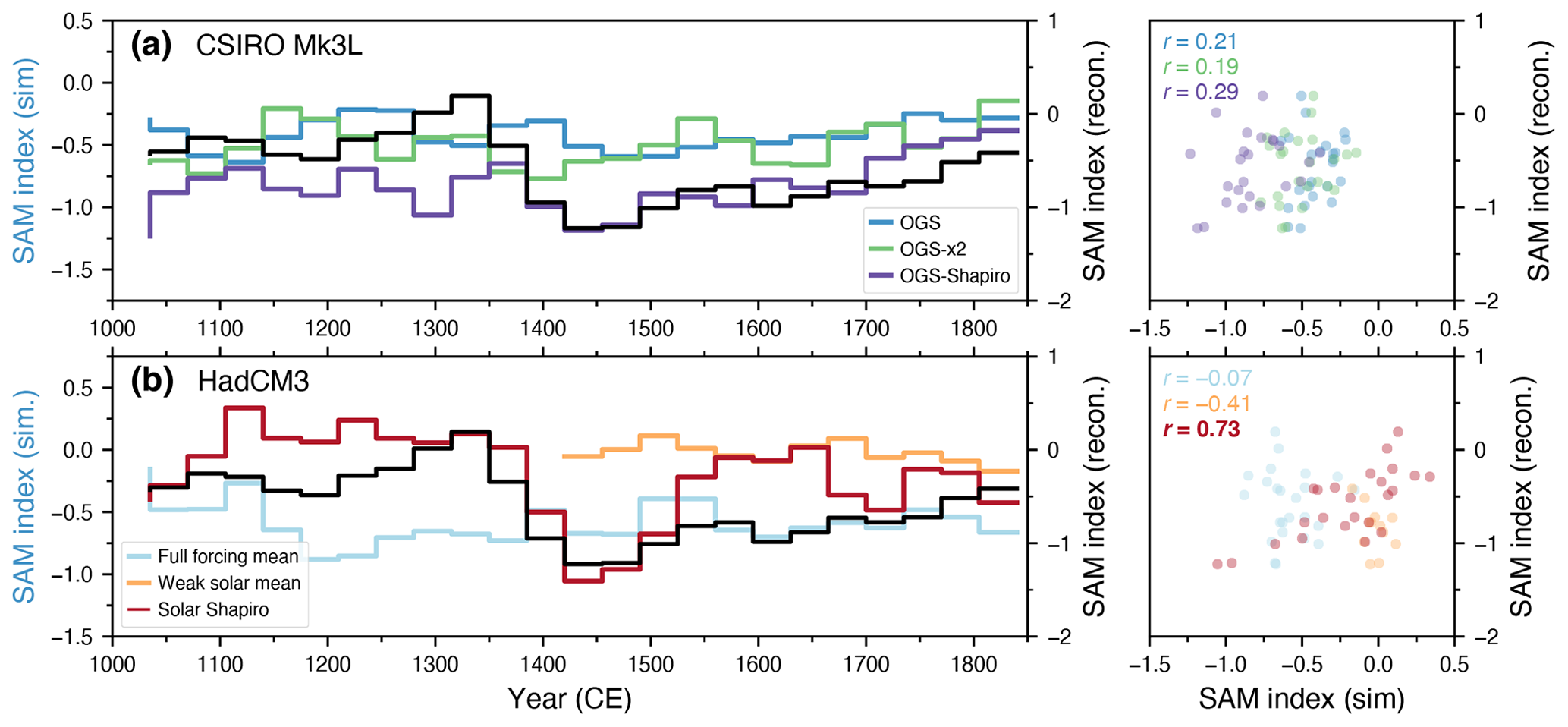
Figure 13Comparison of simulated SAM index and the D18 SAM reconstruction between 1000 and 1900 CE. Time series of the SAM index (70-year moving averages stepped by 35 years; ensemble mean: thick line; ensemble members: thin lines) from transient simulations and SAM reconstruction (70-year moving averages stepped by 35 years) from D18 (black line) for (a) solar transient experiments from CSIRO Mk3L, and (b) simulations from HadCM3 (Schurer et al., 2014), including the full-forcing (blue), weak-solar (orange), and strong-solar (i.e. Shapiro et al., 2011; red) simulations. Note that the solar-forcing simulations from HadCM3 do not include greenhouse gases. Scatter plots show the correlation between 70-year moving averages of the simulated SAM index and the 70-year moving average of the reconstructed SAM index for the ensemble mean, and r values between the simulated and reconstructed SAM index where P<0.05 are shown in bold text.
There have so far been few studies exploring the influence of high-amplitude changes in solar forcing during the last millennium. Research by Schurer et al. (2014) found little influence of stronger solar variability on Northern Hemisphere temperature reconstructions of the last millennium using the HadCM3 model. However, a comparison of the Shapiro et al. (2011) solar-forced run in HadCM3 (Schurer et al., 2014) and our OGS-Shapiro simulation show some similarities in the long-term trends of the SAM index (Fig. 12). In particular, both CSIRO Mk3L and HadCM3 show a large negative excursion in the SAM index around 1450 CE in their strong solar-forcing simulations (Fig. 12, purple and red time series in Fig. 12a and b, respectively). The transient strong solar-forcing simulation from HadCM3 has a significant (P<0.05) correlation with both proxy-based SAM reconstructions (r=0.48 for A14, and r=0.73 for D18). In contrast, last millennium correlations are not significant for the SAM reconstructions with the ensemble mean SAM index in the HadCM3 weak solar-forcing-only simulation and full-forcing (including weak solar-forcing) simulations (Figs. 12b, 13b). The HadCM3 strong solar-forcing experiment thus corroborates our findings using CSIRO Mk3L, indicating that the high-amplitude solar forcing of last millennium simulations has a detectable effect on the annual SAM that improves the agreement between modelled realisations of the SAM index and proxy-based SAM reconstructions.
Solar activity is thought to influence climate, the SAM, and its Northern Hemisphere equivalent – the Northern Annular Mode (NAM) – through either “top-down” (e.g. via changes associated with stratospheric–tropospheric coupling due to ozone- and UV-related stratospheric temperature and wind variations; Gray et al., 2010) or “bottom-up” mechanisms (e.g. through associated changes in sea surface temperature (SST) and ocean heat uptake; Gray et al., 2010; Meehl et al., 2008). Notably, resolving the former mechanism requires climate model simulations using interactive stratospheric chemistry that are computationally expensive to run (and not currently feasible for the last millennium), while bottom-up drivers do not require a well-resolved stratosphere or changes in stratospheric ozone (Meehl et al., 2008). Studies based on observations and/or chemistry-enabled climate models have previously suggested that the SAM (and the NAM) is sensitive to changes in solar activity associated with the 11-year solar cycle (Kuroda et al., 2007; Kuroda and Kodera, 2005; Kuroda and Shibata, 2006; Gray et al., 2010, 2013; Ma et al., 2018; Kuroda, 2018; Arblaster and Meehl, 2006). These studies link variations in the SAM and NAM to changes in stratospheric temperatures and/or stratospheric–tropospheric coupling. For example, during years of higher solar activity, there is a stratospheric extension of the SAM signal (Kuroda and Kodera, 2005), related to a corresponding increase in stratospheric–tropospheric coupling (Kuroda et al., 2007). A similar process is seen for the NAM, though there may be a 2–4-year lagged response of positive NAM following a solar high (Gray et al., 2013; Ma et al., 2018). Solar activity incites variations in stratospheric temperature and winds related to changes in UV irradiance and ozone production, while associated variations in stratospheric–tropospheric coupling result in changes in surface climate (e.g. a top-down forcing) (Gray et al., 2010). This varies from proposed bottom-up mechanisms for solar variations influencing surface climate, which involve changes in SST and ocean heat uptake during periods of increased solar activity, resulting in an increase in latent heat flux and evaporation, which ultimately leads to intensified precipitation along convergence zones, stronger trade winds (Meehl et al., 2008, 2003; Gray et al., 2010), and less heating over the ocean than land (Meehl et al., 2003). Solar forcing may also influence climate through a combination of both top-down and bottom-up mechanisms (Rind et al., 2008), and simulations with both mechanisms working together result in a stronger tropical SST response more similar to observations than simulations with only a single mechanism (Meehl et al., 2009).
As the models examined in this study do not have a well-resolved stratosphere or incorporate interactive stratospheric ozone, we suggest our simulated changes in the SAM are caused by a bottom-up mechanism. We find comparable changes in our increased solar constant experiments to previous studies invoking a bottom-up mechanism, such as an increase in equatorial evaporation and precipitation and a greater increase in land surface temperatures than over the ocean (Fig. 6). Within the atmosphere, our experiments show an increase in solar forcing causes an increase in temperature throughout the tropics, with a larger increase in the upper troposphere than at the surface, cooling in the high-latitude upper troposphere, and a reduced warming in the lower troposphere along 40–60∘ S (Fig. 14b). This increase in temperature is combined with a westerly wind anomaly that spans from the tropical upper troposphere to the high latitudes (∼50∘ S) and extends into the lower troposphere (Fig. 14a) – all of which are similar to the climate effects simulated from an increase in radiative forcing by greenhouse gases (e.g. Kushner et al., 2001; Lim and Simmonds, 2009; Butler et al., 2011). The poleward contraction in the westerly jets around 55∘ S is particularly pronounced in the S+7 and S+35 scenarios, as is the increased meridional temperature gradient (e.g. tropics warming faster than the Southern Ocean), leading to the development of a mean positive SAM state. A decrease in solar forcing results in an approximately inverse pattern: cooling (warming) in the tropical (high-latitude) upper troposphere, cooling across the lower troposphere (Fig. 14b), and a decrease in the zonal wind anomaly across the tropical–high-latitude upper troposphere and into the high-latitude lower troposphere (Fig. 14a). Overall, this indicates a weakening of the westerly jet (i.e. negative zonal wind anomaly around ∼50∘ S) in response to a decrease in solar forcing. Solar forcing affects climate differently to greenhouse gas forcing: solar forcing is primarily shortwave and varies seasonally and spatially, with greater influence in the tropics, while greenhouse gas forcing is more spatially uniform (Meehl et al., 2003). Nevertheless, it is possible that we find a broadly similar tropospheric response, as expected from greenhouse gases, due to the extremely large magnitude of the changes in our solar-forcing experiments combined with exploring transient mean state changes over only the first 200 years (Fig. 4).
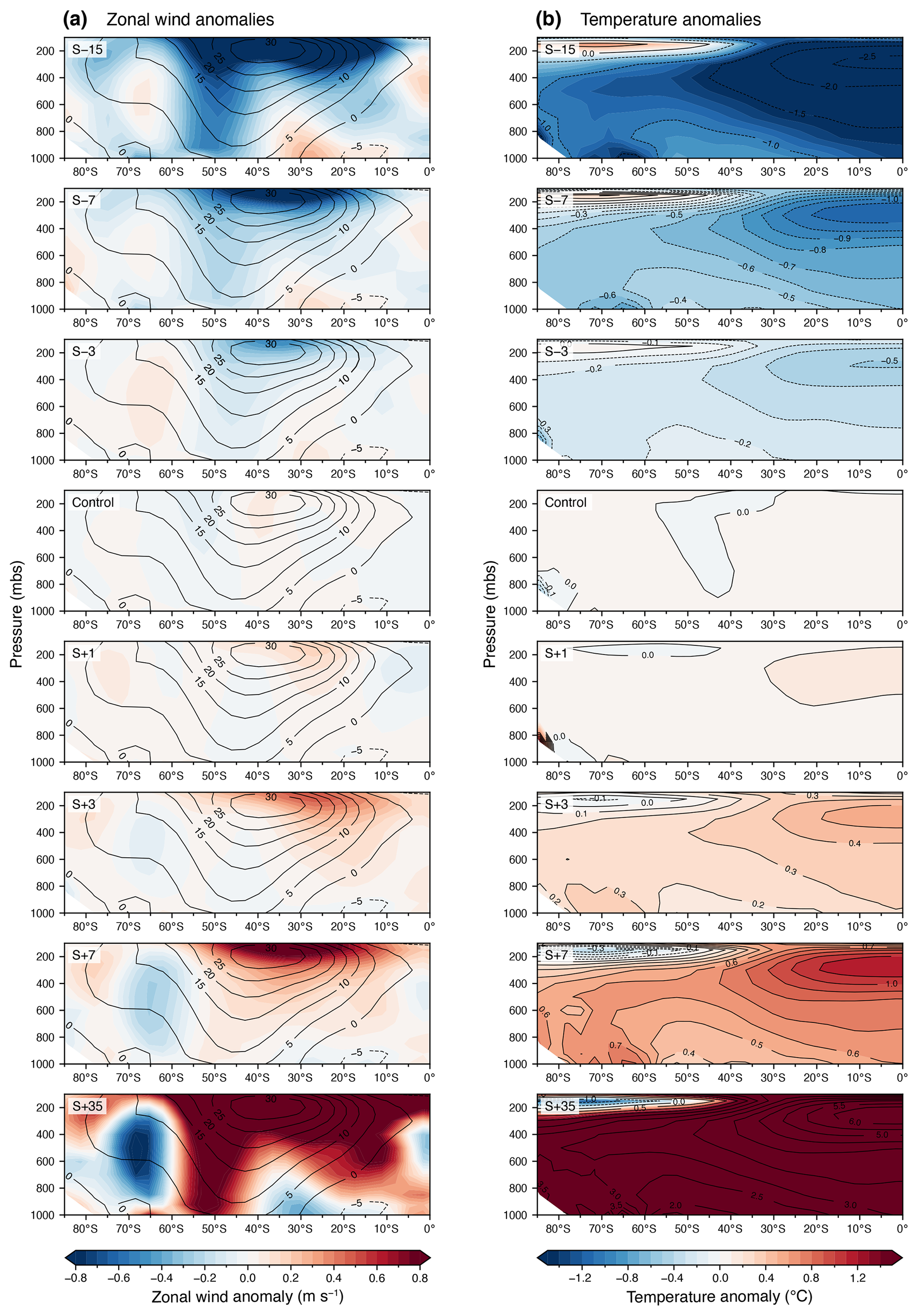
Figure 14Atmospheric profiles for the Southern Hemisphere mean anomalies for the first 200 years of each solar constant experiment. Anomalies are calculated relative to the long-term control. (a) Zonal wind anomalies (shaded) and contours of the control zonal wind (lines). (b) Temperature anomalies (shaded), where contour lines of the temperature anomaly are additionally shown in 0.5 ∘C increments to assist in interpreting S−15 and S+35.
Overall, our findings suggest that the effects of solar forcing on the SAM are not adequately represented in current last millennium climate simulations. It is possible that the reconstructed minimum in the SAM during the 15th century was a response to a minimum in solar irradiance at this time and that this solar response is not reproduced in last millennium simulations that are forced with low-amplitude solar forcing. However, our results do not necessarily imply that solar forcing of the last millennium involved the large amplitude changes of the Shapiro et al. (2011) forcing scenario. The large amplitude of the solar forcing used in our transient experiments was a plausible forcing scenario provided as an option for last millennium experiment design of the Coupled Model Intercomparison Project (Schmidt et al., 2012). However, this strong solar-forcing scenario (i.e. Shapiro et al., 2011) has rarely been applied in last millennium simulations, and it has been argued that the magnitude of TSI change in Shapiro et al. (2011) have been overestimated by a factor of 2 (Judge et al., 2012). Instead, it may be that in climate models that do not have the interactive atmospheric chemistry needed to permit solar impacts on stratospheric ozone, a large amplitude of solar forcing is instead needed to reproduce the last millennium climate impacts on the SAM that were caused by more modest solar-forcing changes. While we cannot rule out the possibility that the strength of the forcing allows our experiments to reproduce changes in the SAM without a realistic representation of all the forcings involved, our strong solar-forcing experiments produce a SAM response that better replicates reconstructed changes in the SAM during the last millennium.
Palaeoclimate reconstructions indicate large changes in the SAM during pre-industrial times that are not replicated in current last millennium climate simulations. We explore changes in solar forcing on the SAM using solar constant and last millennium transient simulations that cover large amplitude solar changes and find that the SAM index significantly decreases (increases) with a decrease (increase) in solar forcing. The magnitude of solar-forcing change required for a significant change in the SAM index is much greater than the most commonly used solar-forcing scenarios for the last millennium. We find an approximately 7 W m−2 decrease in total solar irradiance (or 1.5 W m−2 decrease in radiative forcing) required before the effect of solar forcing on the SAM can be distinguished from the large range of unforced SAM variability. Transient simulations of the last millennium with strong solar forcing result in an improved and significant agreement with proxy-based reconstructions of the SAM. It is plausible that solar forcing may have been an important driver in long-term SAM trends prior to the strong anthropogenic forcing of the 20th and 21st centuries and that current climate model simulations of the last millennium do not adequately represent the effect of solar variability on mid- to high-latitude Southern Hemisphere climate. This may be due to a higher magnitude of solar irradiance changes than is usually applied in last millennium simulations or (more likely) the absence of important physical and chemical processes in coupled global climate models that would allow more moderate changes in solar forcing to have a discernible impact on high-latitude climate.
Data associated with this study can be found at https://doi.org/10.5281/zenodo.6585285 (Wright et al., 2022).
NJA devised the study. CEK performed the solar constant experiments, and NMW and SJP performed the transient simulations. NMW and NJA performed the data analyses with help from GB, and NMW made the figures. NMW wrote the manuscript with contributions from all co-authors.
At least one of the (co-)authors is a member of the editorial board of Climate of the Past. The peer-review process was guided by an independent editor, and the authors also have no other competing interests to declare.
Publisher's note: Copernicus Publications remains neutral with regard to jurisdictional claims in published maps and institutional affiliations.
We thank the reviewers for their constructive comments, which helped improve our manuscript. We thank the Australian Research Council and the Australian Government’s National Environmental Science Program for support. This research was made possible by computational resources provided by the National Computational Infrastructure, including resources awarded through the NCI and ANU merit allocation schemes.
This research has been supported by funding from the Australian Research Council (grant nos. CE170100023, DP140102059, FT160100029, and SR200100008) and the Australian Government under the National Environmental Science Program Climate Systems Hub.
This paper was edited by Elizabeth Thomas and reviewed by two anonymous referees.
Abram, N. J., Mulvaney, R., Vimeux, F., Phipps, S. J., Turner, J., and England, M. H.: Evolution of the Southern Annular Mode during the past millennium, Nat. Clim. Change, 4, 564–569, 2014.
Arblaster, J. M. and Meehl, G. A.: Contributions of external forcings to southern annular mode trends, J. Climate, 19, 2896–2905, 2006.
Arblaster, J. M., Meehl, G. A., and Karoly, D. J.: Future climate change in the Southern Hemisphere: Competing effects of ozone and greenhouse gases, Geophys. Res. Lett., 38, L02701, https://doi.org/10.1029/2010GL045384, 2011.
Banerjee, A., Fyfe, J. C., Polvani, L. M., Waugh, D., and Chang, K.-L.: A pause in Southern Hemisphere circulation trends due to the Montreal Protocol, Nature, 579, 544–548, 2020.
Barnes, E. A. and Polvani, L.: Response of the midlatitude jets, and of their variability, to increased greenhouse gases in the CMIP5 models, J. Climate, 26, 7117–7135, 2013.
Brehm, N., Bayliss, A., Christl, M., Synal, H.-A., Adolphi, F., Beer, J., Kromer, B., Muscheler, R., Solanki, S. K., and Usoskin, I.: Eleven-year solar cycles over the last millennium revealed by radiocarbon in tree rings, Nat. Geosci., 14, 10–15, 2021.
Butler, A. H., Thompson, D. W., and Birner, T.: Isentropic slopes, downgradient eddy fluxes, and the extratropical atmospheric circulation response to tropical tropospheric heating, J. Atmos. Sci., 68, 2292–2305, 2011.
Crosta, X., Etourneau, J., Orme, L. C., Dalaiden, Q., Campagne, P., Swingedouw, D., Goosse, H., Massé, G., Miettinen, A., McKay, R. M., Dunbar, R. B., Escutia, C., and Ikehara, M.: Multi-decadal trends in Antarctic sea-ice extent driven by ENSO–SAM over the last 2,000 years, Nat. Geosci., 14, 156–160, https://doi.org/10.1038/s41561-021-00697-1, 2021.
Dätwyler, C., Neukom, R., Abram, N. J., Gallant, A. J. E., Grosjean, M., Jacques-Coper, M., Karoly, D. J., and Villalba, R.: Teleconnection stationarity, variability and trends of the Southern Annular Mode (SAM) during the last millennium, Clim. Dynam., 51, 2321–2339, https://doi.org/10.1007/s00382-017-4015-0, 2018.
Fan, K. and Wang, H.: Antarctic oscillation and the dust weather frequency in North China, Geophys. Res. Lett., 31, L10201, https://doi.org/10.1029/2004GL019465, 2004.
Fogt, R. L. and Marshall, G. J.: The Southern Annular Mode: variability, trends, and climate impacts across the Southern Hemisphere, WIREs Clim. Change, 11, e652, https://doi.org/10.1002/wcc.652, 2020.
Fogt, R. L., Perlwitz, J., Monaghan, A. J., Bromwich, D. H., Jones, J. M., and Marshall, G. J.: Historical SAM variability. Part II: Twentieth-century variability and trends from reconstructions, observations, and the IPCC AR4 models, J. Climate, 22, 5346–5365, 2009.
Fyfe, J., Boer, G., and Flato, G.: The Arctic and Antarctic Oscillations and their projected changes under global warming, Geophys. Res. Lett., 26, 1601–1604, 1999.
Gillett, N. and Fyfe, J.: Annular mode changes in the CMIP5 simulations, Geophys. Res. Lett., 40, 1189-1193, 2013.
Gillett, N. P. and Thompson, D. W.: Simulation of recent Southern Hemisphere climate change, Science, 302, 273–275, 2003.
Gillett, N. P., Kell, T. D., and Jones, P.: Regional climate impacts of the Southern Annular Mode, Geophys. Res. Lett., 33, L23704, https://doi.org/10.1029/2006GL027721, 2006.
Gong, D. and Wang, S.: Definition of Antarctic oscillation index, Geophys. Res. Lett., 26, 459–462, 1999.
Goyal, R., Sen Gupta, A., Jucker, M., and England, M. H.: Historical and projected changes in the Southern Hemisphere surface westerlies, Geophys. Res. Lett., 48, e2020GL090849, https://doi.org/10.1029/2020GL090849, 2021.
Gray, L. J., Beer, J., Geller, M., Haigh, J. D., Lockwood, M., Matthes, K., Cubasch, U., Fleitmann, D., Harrison, G., and Hood, L.: Solar influences on climate, Rev. Geophys., 48, RG4001, https://doi.org/10.1029/2009RG000282, 2010.
Gray, L. J., Scaife, A. A., Mitchell, D. M., Osprey, S., Ineson, S., Hardiman, S., Butchart, N., Knight, J., Sutton, R., and Kodera, K.: A lagged response to the 11 year solar cycle in observed winter Atlantic/European weather patterns, J. Geophys. Res.-Atmos., 118, 13405–413420, 2013.
Grise, K. M., Polvani, L. M., Tselioudis, G., Wu, Y., and Zelinka, M. D.: The ozone hole indirect effect: Cloud-radiative anomalies accompanying the poleward shift of the eddy-driven jet in the Southern Hemisphere, Geophys. Res. Lett., 40, 3688–3692, 2013.
Hendon, H. H., Thompson, D. W., and Wheeler, M. C.: Australian rainfall and surface temperature variations associated with the Southern Hemisphere annular mode, J. Climate, 20, 2452–2467, 2007.
Hessl, A., Allen, K. J., Vance, T., Abram, N. J., and Saunders, K. M.: Reconstructions of the southern annular mode (SAM) during the last millennium, Prog. Phys. Geog., 41, 834–849, 2017.
Huiskamp, W. and McGregor, S.: Quantifying Southern Annular Mode paleo-reconstruction skill in a model framework, Clim. Past, 17, 1819–1839, https://doi.org/10.5194/cp-17-1819-2021, 2021.
Jones, J. M., Fogt, R. L., Widmann, M., Marshall, G. J., Jones, P. D., and Visbeck, M.: Historical SAM variability. Part I: Century-length seasonal reconstructions, J. Climate, 22, 5319–5345, 2009.
Jones, J. M., Gille, S. T., Goosse, H., Abram, N. J., Canziani, P. O., Charman, D. J., Clem, K. R., Crosta, X., de Lavergne, C., and Eisenman, I.: Assessing recent trends in high-latitude Southern Hemisphere surface climate, Nat. Clim. Change, 6, 917–926, 2016.
Judge, P. G., Lockwood, G. W., Radick, R. R., Henry, G. W., Shapiro, A. I., Schmutz, W., and Lindsey, C.: Confronting a solar irradiance reconstruction with solar and stellar data, Astron. Astrophys., 544, A88, https://doi.org/10.1051/0004-6361/201218903, 2012.
Jungclaus, J. H., Bard, E., Baroni, M., Braconnot, P., Cao, J., Chini, L. P., Egorova, T., Evans, M., González-Rouco, J. F., Goosse, H., Hurtt, G. C., Joos, F., Kaplan, J. O., Khodri, M., Klein Goldewijk, K., Krivova, N., LeGrande, A. N., Lorenz, S. J., Luterbacher, J., Man, W., Maycock, A. C., Meinshausen, M., Moberg, A., Muscheler, R., Nehrbass-Ahles, C., Otto-Bliesner, B. I., Phipps, S. J., Pongratz, J., Rozanov, E., Schmidt, G. A., Schmidt, H., Schmutz, W., Schurer, A., Shapiro, A. I., Sigl, M., Smerdon, J. E., Solanki, S. K., Timmreck, C., Toohey, M., Usoskin, I. G., Wagner, S., Wu, C.-J., Yeo, K. L., Zanchettin, D., Zhang, Q., and Zorita, E.: The PMIP4 contribution to CMIP6 – Part 3: The last millennium, scientific objective, and experimental design for the PMIP4 past1000 simulations, Geosci. Model Dev., 10, 4005–4033, https://doi.org/10.5194/gmd-10-4005-2017, 2017.
Kuroda, Y.: On the Origin of the Solar Cycle Modulation of the Southern Annular Mode, J. Geophys. Res.-Atmos., 123, 1959–1969, https://doi.org/10.1002/2017JD027091, 2018.
Kuroda, Y. and Kodera, K.: Solar cycle modulation of the Southern Annular Mode, Geophys. Res. Lett., 32, L13802, https://doi.org/10.1029/2005GL022516, 2005.
Kuroda, Y. and Shibata, K.: Simulation of solar-cycle modulation of the Southern Annular Mode using a chemistry-climate model, Geophys. Res. Lett., 33, L05703, https://doi.org/10.1029/2005GL025095, 2006.
Kuroda, Y., Deushi, M., and Shibata, K.: Role of solar activity in the troposphere-stratosphere coupling in the Southern Hemisphere winter, Geophys. Res. Lett., 34, L21704, https://doi.org/10.1029/2007GL030983, 2007.
Kushner, P. J., Held, I. M., and Delworth, T. L.: Southern Hemisphere atmospheric circulation response to global warming, J. Climate, 14, 2238–2249, 2001.
Lean, J. and Rind, D.: Climate forcing by changing solar radiation, J. Climate, 11, 3069–3094, https://doi.org/10.1175/1520-0442(1998)011<3069:CFBCSR>2.0.CO;2, 1998.
Lim, E.-P. and Simmonds, I.: Effect of tropospheric temperature change on the zonal mean circulation and SH winter extratropical cyclones, Clim. Dynam., 33, 19–32, 2009.
Lu, H., Jarvis, M. J., Gray, L. J., and Baldwin, M. P.: High- and low-frequency 11-year solar cycle signatures in the Southern Hemispheric winter and spring, Q. J. Roy. Meteor. Soc., 137, 1641–1656, https://doi.org/10.1002/qj.852, 2011.
Ma, H., Chen, H., Gray, L., Zhou, L., Li, X., Wang, R., and Zhu, S.: Changing response of the North Atlantic/European winter climate to the 11 year solar cycle, Environ. Res. Lett., 13, 034007, https://doi.org/10.1088/1748-9326/aa9e94, 2018.
Marshall, G. J.: Trends in the Southern Annular Mode from Observations and Reanalyses, J. Climate, 16, 4134–4143, https://doi.org/10.1175/1520-0442(2003)016<4134:Titsam>2.0.Co;2, 2003.
Meehl, G. A., Washington, W. M., Wigley, T., Arblaster, J. M., and Dai, A.: Solar and greenhouse gas forcing and climate response in the twentieth century, J. Climate, 16, 426–444, 2003.
Meehl, G. A., Arblaster, J. M., Branstator, G., and van Loon, H.: A Coupled Air–Sea Response Mechanism to Solar Forcing in the Pacific Region, J. Climate, 21, 2883–2897, https://doi.org/10.1175/2007jcli1776.1, 2008.
Meehl, G. A., Arblaster, J. M., Matthes, K., Sassi, F., and van Loon, H.: Amplifying the Pacific climate system response to a small 11-year solar cycle forcing, Science, 325, 1114–1118, 2009.
Meehl, G. A., Washington, W. M., Arblaster, J. M., Hu, A., Teng, H., Tebaldi, C., Sanderson, B. N., Lamarque, J.-F., Conley, A., and Strand, W. G.: Climate system response to external forcings and climate change projections in CCSM4, J. Climate, 25, 3661–3683, 2012.
Miller, R. L., Schmidt, G. A., and Shindell, D. T.: Forced annular variations in the 20th century Intergovernmental Panel on Climate Change Fourth Assessment Report models, J. Geophys. Res., 111, D18101, https://doi.org/10.1029/2005JD006323, 2006.
Neukom, R., Schurer, A. P., Steiger, N. J., and Hegerl, G. C.: Possible causes of data model discrepancy in the temperature history of the last Millennium, Scientific Reports, 8, 7572, https://doi.org/10.1038/s41598-018-25862-2, 2018.
Ortega, P., Lehner, F., Swingedouw, D., Masson-Delmotte, V., Raible, C. C., Casado, M., and Yiou, P.: A model-tested North Atlantic Oscillation reconstruction for the past millennium, Nature, 523, 71–74, https://doi.org/10.1038/nature14518, 2015.
Otto-Bliesner, B. L., Brady, E. C., Fasullo, J., Jahn, A., Landrum, L., Stevenson, S., Rosenbloom, N., Mai, A., and Strand, G.: Climate Variability and Change since 850 CE: An Ensemble Approach with the Community Earth System Model, B. Am. Meteorol. Soc., 97, 735–754, https://doi.org/10.1175/bams-d-14-00233.1, 2016.
PAGES2k Consortium: A global multiproxy database for temperature reconstructions of the Common Era, Scientific Data, 4, 170088, https://doi.org/10.1038/sdata.2017.88, 2017.
PAGES 2k Consortium: Consistent multidecadal variability in global temperature reconstructions and simulations over the Common Era, Nat. Geosci., 12, 643–649, https://doi.org/10.1038/s41561-019-0400-0, 2019.
PAGES 2k-PMIP3 group: Continental-scale temperature variability in PMIP3 simulations and PAGES 2k regional temperature reconstructions over the past millennium, Clim. Past, 11, 1673–1699, https://doi.org/10.5194/cp-11-1673-2015, 2015.
Phipps, S. J., Rotstayn, L. D., Gordon, H. B., Roberts, J. L., Hirst, A. C., and Budd, W. F.: The CSIRO Mk3L climate system model version 1.0 – Part 1: Description and evaluation, Geosci. Model Dev., 4, 483–509, https://doi.org/10.5194/gmd-4-483-2011, 2011.
Phipps, S. J., Rotstayn, L. D., Gordon, H. B., Roberts, J. L., Hirst, A. C., and Budd, W. F.: The CSIRO Mk3L climate system model version 1.0 – Part 2: Response to external forcings, Geosci. Model Dev., 5, 649–682, https://doi.org/10.5194/gmd-5-649-2012, 2012.
Phipps, S. J., McGregor, H. V., Gergis, J., Gallant, A. J. E., Neukom, R., Stevenson, S., Ackerley, D., Brown, J. R., Fischer, M. J., and van Ommen, T. D.: Paleoclimate Data–Model Comparison and the Role of Climate Forcings over the Past 1500 Years, J. Climate, 26, 6915–6936, https://doi.org/10.1175/jcli-d-12-00108.1, 2013.
Polvani, L. M., Waugh, D. W., Correa, G. J., and Son, S.-W.: Stratospheric ozone depletion: The main driver of twentieth-century atmospheric circulation changes in the Southern Hemisphere, J. Climate, 24, 795–812, 2011a.
Polvani, L. M., Waugh, D. W., Correa, G. J. P., and Son, S.-W.: Stratospheric Ozone Depletion: The Main Driver of Twentieth-Century Atmospheric Circulation Changes in the Southern Hemisphere, J. Climate, 24, 795–812, https://doi.org/10.1175/2010jcli3772.1, 2011b.
Raphael, M. N. and Holland, M. M.: Twentieth century simulation of the southern hemisphere climate in coupled models. Part 1: large scale circulation variability, Clim. Dynam., 26, 217–228, https://doi.org/10.1007/s00382-005-0082-8, 2006.
Rind, D., Lean, J., Lerner, J., Lonergan, P., and Leboissitier, A.: Exploring the stratospheric/tropospheric response to solar forcing, J. Geophys. Res., 113, D24103, https://doi.org/10.1029/2008JD010114, 2008.
Roscoe, H. K. and Haigh, J. D.: Influences of ozone depletion, the solar cycle and the QBO on the Southern Annular Mode, Q. J. Roy. Meteor. Soc., 133, 1855–1864, https://doi.org/10.1002/qj.153, 2007.
Saunders, K. M., Roberts, S. J., Perren, B., Butz, C., Sime, L., Davies, S., Van Nieuwenhuyze, W., Grosjean, M., and Hodgson, D. A.: Holocene dynamics of the Southern Hemisphere westerly winds and possible links to CO2 outgassing, Nat. Geosci., 11, 650–655, https://doi.org/10.1038/s41561-018-0186-5, 2018.
Schmidt, G. A., Jungclaus, J. H., Ammann, C. M., Bard, E., Braconnot, P., Crowley, T. J., Delaygue, G., Joos, F., Krivova, N. A., Muscheler, R., Otto-Bliesner, B. L., Pongratz, J., Shindell, D. T., Solanki, S. K., Steinhilber, F., and Vieira, L. E. A.: Climate forcing reconstructions for use in PMIP simulations of the last millennium (v1.0), Geosci. Model Dev., 4, 33–45, https://doi.org/10.5194/gmd-4-33-2011, 2011.
Schmidt, G. A., Jungclaus, J. H., Ammann, C. M., Bard, E., Braconnot, P., Crowley, T. J., Delaygue, G., Joos, F., Krivova, N. A., Muscheler, R., Otto-Bliesner, B. L., Pongratz, J., Shindell, D. T., Solanki, S. K., Steinhilber, F., and Vieira, L. E. A.: Climate forcing reconstructions for use in PMIP simulations of the Last Millennium (v1.1), Geosci. Model Dev., 5, 185–191, https://doi.org/10.5194/gmd-5-185-2012, 2012.
Schurer, A. P., Tett, S. F., and Hegerl, G. C.: Small influence of solar variability on climate over the past millennium, Nat. Geosci., 7, 104–108, 2014.
Sen Gupta, A. and England, M. H.: Coupled ocean–atmosphere–ice response to variations in the southern annular mode, J. Climate, 19, 4457–4486, 2006.
Shapiro, A., Schmutz, W., Rozanov, E., Schoell, M., Haberreiter, M., Shapiro, A., and Nyeki, S.: A new approach to the long-term reconstruction of the solar irradiance leads to large historical solar forcing, Astron. Astrophys., 529, A67, https://doi.org/10.1051/0004-6361/201016173, 2011.
Shindell, D. T. and Schmidt, G. A.: Southern Hemisphere climate response to ozone changes and greenhouse gas increases, Geophys. Res. Lett., 31, L18209, https://doi.org/10.1029/2004GL020724, 2004.
Son, S. W., Tandon, N. F., Polvani, L. M., and Waugh, D. W.: Ozone hole and Southern Hemisphere climate change, Geophys. Res. Lett., 36, L15705, https://doi.org/10.1029/2009GL038671, 2009.
Steinhilber, F., Beer, J., and Fröhlich, C.: Total solar irradiance during the Holocene, Geophys. Res. Lett., 36, L19704, https://doi.org/10.1029/2009GL040142, 2009.
Swart, N. and Fyfe, J. C.: Observed and simulated changes in the Southern Hemisphere surface westerly wind-stress, Geophys. Res. Lett., 39, L16711, https://doi.org/10.1029/2012GL052810, 2012.
Thompson, D. W. and Solomon, S.: Interpretation of recent Southern Hemisphere climate change, Science, 296, 895–899, 2002.
Thompson, D. W. and Wallace, J. M.: Annular modes in the extratropical circulation. Part I: Month-to-month variability, J. Climate, 13, 1000–1016, 2000.
Thompson, D. W. J., Solomon, S., Kushner, P. J., England, M. H., Grise, K. M., and Karoly, D. J.: Signatures of the Antarctic ozone hole in Southern Hemisphere surface climate change, Nat. Geosci., 4, 741–749, https://doi.org/10.1038/ngeo1296, 2011.
Villalba, R., Lara, A., Masiokas, M. H., Urrutia, R., Luckman, B. H., Marshall, G. J., Mundo, I. A., Christie, D. A., Cook, E. R., and Neukom, R.: Unusual Southern Hemisphere tree growth patterns induced by changes in the Southern Annular Mode, Nat. Geosci., 5, 793–798, 2012.
Visbeck, M.: A station-based southern annular mode index from 1884 to 2005, J. Climate, 22, 940–950, 2009.
Wang, G. and Cai, W.: Climate-change impact on the 20th-century relationship between the Southern Annular Mode and global mean temperature, Scientific Reports, 3, 1–6, 2013.
Wang, Y.-M., Lean, J., and Sheeley Jr, N.: Modeling the Sun's magnetic field and irradiance since 1713, Astrophys. J., 625, 522, https://doi.org/10.1086/429689, 2005.
Wright, N. M., Krause, C. E., Phipps, S. J., Boschat, G., and Abram, N. J.: Influence of long-term changes in solar irradiance forcing on the Southern Annular Mode, Zenodo [data set], https://doi.org/10.5281/zenodo.6585285, 2022.
Yang, D., Arblaster, J. M., Meehl, G. A., England, M. H., Lim, E.-P., Bates, S., and Rosenbloom, N.: Role of tropical variability in driving decadal shifts in the Southern Hemisphere summertime eddy-driven jet, J. Climate, 33, 5445–5463, 2020.
Zheng, F., Li, J., Clark, R. T., and Nnamchi, H. C.: Simulation and projection of the Southern Hemisphere annular mode in CMIP5 models, J. Climate, 26, 9860–9879, 2013.