the Creative Commons Attribution 4.0 License.
the Creative Commons Attribution 4.0 License.
 | 14 Apr 2021
Snapshots of mean ocean temperature over the last 700 000 years using noble gases in the EPICA Dome C ice core
Marcel Haeberli
Daniel Baggenstos
Jochen Schmitt
Markus Grimmer
Adrien Michel
Thomas Kellerhals
Hubertus Fischer
Together with the latent heat stored in glacial ice sheets, the ocean heat uptake carries the lion's share of glacial–interglacial changes in the planetary heat content, but little direct information on the global mean ocean temperature (MOT) is available to constrain the ocean temperature response to glacial–interglacial climate perturbations. Using ratios of noble gases and molecular nitrogen trapped in the Antarctic EPICA Dome C ice core, we are able to reconstruct MOT for peak glacial and interglacial conditions during the last 700 000 years and explore the differences between these extrema. To this end, we have to correct the noble gas ratios for gas transport effects in the firn column and gas loss fractionation processes of the samples after ice core retrieval using the full elemental matrix of N2, Ar, Kr, and Xe in the ice and their individual isotopic ratios. The reconstructed MOT in peak glacials is consistently about 3.3 ± 0.4 ∘C cooler compared to the Holocene. Lukewarm interglacials before the Mid-Brunhes Event 450 kyr ago are characterized by 1.6 ± 0.4 ∘C lower MOT than the Holocene; thus, glacial–interglacial amplitudes were only about 50 % of those after the Mid-Brunhes Event, in line with the reduced radiative forcing by lower greenhouse gas concentrations and their Earth system feedbacks. Moreover, we find significantly increased MOTs at the onset of Marine Isotope Stage 5.5 and 9.3, which are coeval with CO2 and CH4 overshoots at that time. We link these CO2 and CH4 overshoots to a resumption of the Atlantic Meridional Overturning Circulation, which is also the starting point of the release of heat previously accumulated in the ocean during times of reduced overturning.
- Article
(4280 KB) - Full-text XML
- BibTeX
- EndNote


Over the last million years, Earth's climate has experienced pronounced changes in global ice volume (Bintanja et al., 2005) and hence sea level, accompanied by significant temperature changes between cold glacials and warmer interglacials. These temperature changes are observed with different amplitudes both on land (EPICA community members, 2004; Tzedakis et al., 2006; Melles et al., 2012) and in the ocean (Elderfield et al., 2012; Shakun et al., 2012, 2015). In particular, due to the large size and heat capacity of the ocean reservoir, global mean ocean temperature (MOT) changes (together with the latent heat stored in waxing ice sheets) represent an integrated signal of Earth's energy imbalance in the past (Baggenstos et al., 2019). For example, today, the global ocean is taking up about 90 % of the excess heat from anthropogenic global warming, dominating the current changes in the planetary energy budget (Gleckler et al., 2016; von Schuckmann et al., 2020).
In contrast to today's warming, where radiative forcing is caused through anthropogenic emissions of CO2, past climate cycles are generally believed to have been driven by orbital changes in the latitudinal and seasonal distribution of incoming solar radiation (Milankovic, 1941), with changing greenhouse gas concentrations representing an important amplifying feedback. Only recently did Tzedakis et al. (2017) propose a simple rule for the occurrence of full deglaciations based on the amount of effective incoming energy flux (defined as the caloric summer half-year insolation at 65∘ N corrected by a term that takes into account the time elapsed since the previous deglaciation). While this rule is in agreement with the occurrence of all full deglaciations over the last million years, it does not intend to predict differences between individual interglacials in ice volume and climate. For example, Marine Isotope Stage (MIS) 11 is characterized by a very long interval of interglacial conditions and a sea level at least equally high as in MIS 5.5 and likely more than 6 m higher than in the Holocene (Dutton et al., 2015) . However, its effective energy is just reaching the threshold suggested by Tzedakis et al. (2017), while MIS 5.5 exhibits the largest effective energy over the last 800 kyr and the second largest over the last 2.6 Myr (Tzedakis et al., 2017). Moreover, lukewarm interglacials (i.e., interglacials significantly colder than the Holocene with increased ice volume) were observed in local temperature reconstructions and global sea level (EPICA community members, 2004; PAGES Past Interglacials Working Group, 2016; Shakun et al., 2015; Elderfield et al., 2012) in the time interval 800–450 kyr BP (before present; present is defined as 1950). Again, the effective energy during these lukewarm interglacials is not systematically lower than for the subsequent interglacials, requiring additional energetic or radiative changes in the climate system to explain the difference between the individual interglacials. MOT may play an important role in explaining these features, as a higher ocean heat content could represent a compensating mechanism for the excess energy not used for the melting of the larger remnant ice sheets during lukewarm interglacials. The opposite is also true: if lower MOT parallels larger ice volume during lukewarm interglacials, changes in the radiative balance of the Earth are required to explain the differences between the interglacials before and after 450 kyr BP.
Quantitative estimates of the integrated heat content of the entire ocean are required to answer these questions. However, obtaining a representative estimate of the whole-ocean heat content represents a formidable challenge (Hoffman et al., 2017; Shakun et al., 2015). Marine sediments are available for many but not all ocean areas and record only local sea surface conditions or deep-ocean temperatures at the coring site. Moreover, the proxy temperature information gained from marine sediments may be affected by biological processes, sea level changes, or limited precision, especially for cold deep-ocean temperatures. Finally, obtaining globally representative MOT from individual marine archives requires the compilation of a globally representative set of marine sediment cores, including rigorous cross-dating of all the records, which is difficult for the pre-14C period.
The measurement of atmospheric noble gases trapped in Antarctic ice provides a unique opportunity to reconstruct changes in MOT independently from marine records (Craig and Wiens, 1996; Bereiter et al., 2018b; Headly and Severinghaus, 2007; Ritz et al., 2011) and may overcome these limitations. Changes in the atmospheric concentrations of xenon, krypton, and nitrogen (we liberally add N2 to the noble gases, as its atmospheric residence time amounts to tens of millions of years) mirror the anomalies in total ocean heat content, as they are driven by changes in their temperature-dependent physical solubilities in ocean water. This allows us to reconstruct MOT in the past from the noble gas composition of a single ice core sample. A minor exception is the small amount of geothermal heating of ocean water, which is not connected to a noble gas change. Note that the MOT at a given time in the past represents a snapshot of the heat (and noble gas) content of all water parcels of the ocean and thus integrates over water bodies with different ventilation ages. Importantly, MOT is therefore not directly linked to mean global sea surface temperature at the same time, a point that has caused some confusion in the past.
Here we extend previous efforts in reconstructing MOT using noble gases in ice cores (Bereiter et al., 2018b; Baggenstos et al., 2019; Shackleton et al., 2020), which were limited to the last and penultimate glacial terminations, by reconstructing the glacial–interglacial MOT range for snapshots of all glacial and interglacial intervals over the last 700 000 years using the EPICA Dome C (EDC) ice core. To obtain quantitative MOT values, large corrections of the raw data for physical transport processes in the firn have to be applied, which affect the precision and accuracy of the MOT data. Moreover, gas fractionation processes in the ice between bubbles and clathrates in connection with potential post-coring gas loss have been observed (Bender et al., 1995), which have to be unambiguously identified to allow us to derive an unbiased MOT estimate, as described in detail in this study. Despite these corrections, we are able to derive quantitative MOT values from high-precision measurements of noble gas mixing ratios in the EDC ice core.
The paper is organized as follows: in Sect. 2 we describe the overall analytical procedure to obtain noble gas isotopic and elemental ratios with the associated uncertainty as well as the corrections that have to be applied to correct for systematic transport effects in the firn column. As EDC is a very low-accumulation site, which exhibits a permanent firn temperature gradient larger than 1 ∘C, thermal diffusion has to be precisely quantified. Moreover, we describe in detail for the first time the correction of kinetic fractionation by non-diffusive transport, adding an additional layer of complexity and uncertainty. Another process acting on the noble gas composition in the EDC ice core is post-coring gas loss that affects samples from the bubble–clathrate transition zone and, more severely, fully clathrated ice from the deepest ice at Dome C, which is close to the pressure melting point. These effects are described in detail for the first time in Sect. 3, and a hypothesis on how these lead to systematic noble gas fractionation is presented. For the reader only interested in the final results of our MOT reconstruction over the last 700 kyr and their discussion, we refer directly to Sect. 4 and the Conclusions section.
2.1 Determination of noble gas elemental and isotopic ratios in ice cores
The data set presented here consists of 88 EDC ice samples (39 samples span the last 40 kyr, and 49 samples are from MIS 5 to MIS 17; Baggenstos et al., 2019) that were analyzed at the University of Bern. In order to test the representativeness of our EDC MOT data, 4 samples from the EPICA Dronning Maud Land (EDML) ice core, 4 samples from the Greenland Ice Core Project (GRIP) ice core, 4 samples from the Greenland NEEM ice core, 4 samples from the Antarctic Talos Dome ice core, and 13 blue ice samples from Taylor Glacier were measured. The Taylor Glacier samples stem from a lab intercomparison with the Scripps Institution of Oceanography in San Diego and showed excellent agreement within the analytical uncertainties between the two labs. Two samples from EDC (age > 700 kyr BP) were discarded due to bad ice quality together with drill fluid contamination, and one sample was rejected due to a procedural problem.
The gas extraction and processing broadly follow the method described in detail by Bereiter et al. (2018a). In short, after shaving off the outer surface ∼600 g of ice is melt-extracted (equivalent to ∼55 mL at the standard temperature and pressure (STP) of extracted air) and the released air is quantitatively frozen into stainless-steel dip tubes in a helium exchange cryostat. To equilibrate the sample and to avoid fractionation by thermal gradients in the dip tube, the dip tubes are kept for at least 10 h in a ventilated isothermal box. The samples are then split into two aliquots. The larger (∼53 mL STP) aliquot is exposed to a getter alloy at 900 ∘C to remove all reactive gases and is analyzed in a peak-jumping routine on a Thermo Finnigan MAT 253 dual-inlet isotope ratio mass spectrometer (IRMS) for the isotopic ratios of xenon, krypton, and argon as well as their elemental ratios. The smaller aliquot (∼2 mL STP) is passed through a CO2 trap and measured on a Thermo Finnigan MAT Delta V dual-inlet IRMS in parallel for argon, oxygen, and nitrogen isotopes and their elemental ratios. The measurements were corrected for pressure imbalance and chemical slope according to the procedure described in Severinghaus et al. (2003). All data are reported in the delta notation with respect to a modern atmosphere standard collected outside the lab in Bern, Switzerland. Note that this atmospheric value reflects the current dissolution equilibrium of the studied gases between the atmosphere and the global ocean; this atmospheric standard is not subject to fractionation processes in the firn that affect air samples from ice cores. Accordingly, in the absence of any long-term changes in the total abundance of noble gas isotopes in the combined atmosphere and ocean reservoirs, each determined ice core value provides a measure of the difference in the ocean heat content at the age of the sample relative to today.
Table 1Long-term reproducibility of the analyses (1 standard deviation) derived from 51 measurements of outside air on the MAT 253 and 46 measurements of outside air on the Delta V Plus.
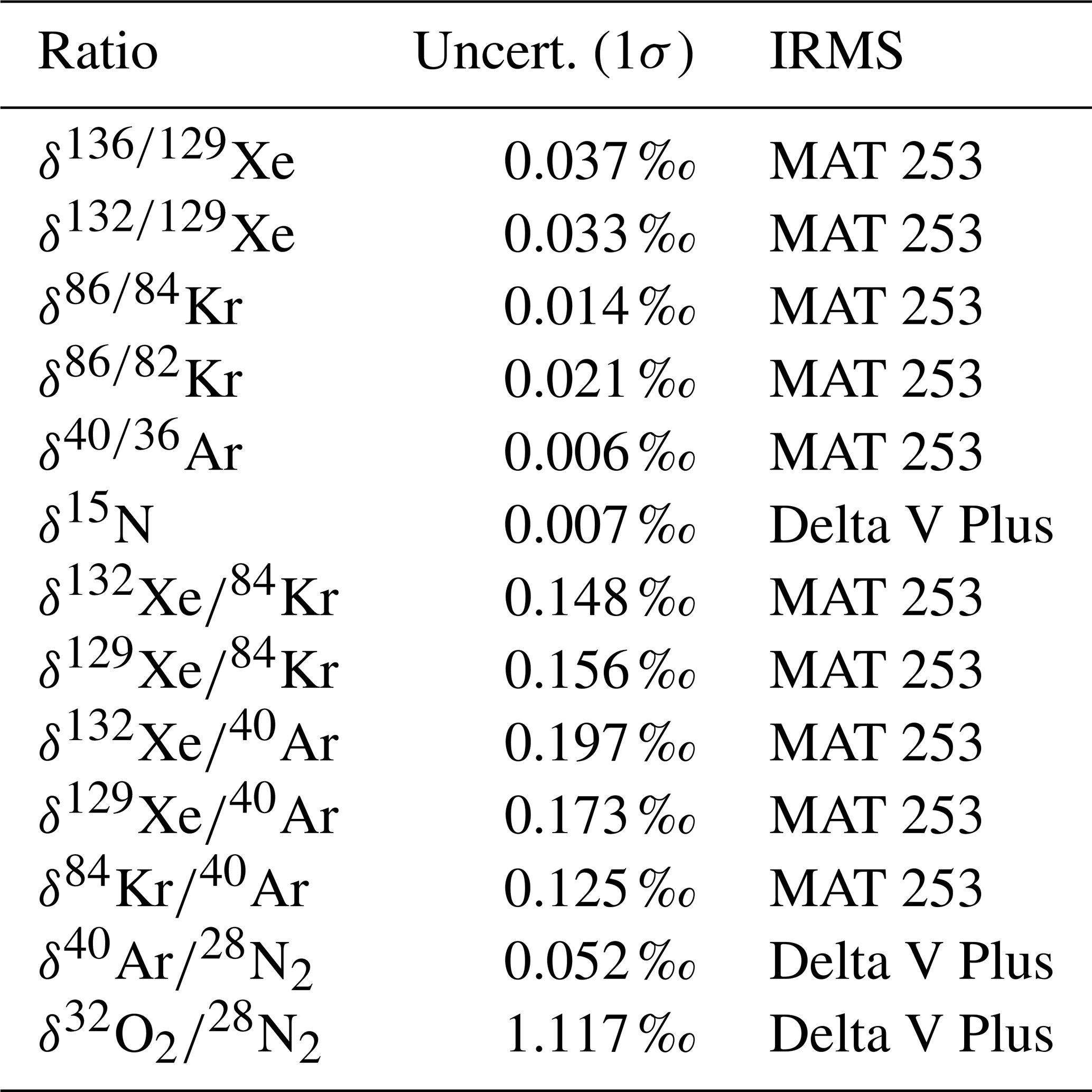
The long-term reproducibility of our system, which was determined using outside air samples, may be found in Table 1. When normalized to one unit of mass difference, all isotopic ratios can be quantified to better than 10 per meg with uncertainties as low as 5 per meg per difference mass unit for , 7 per meg per difference mass unit for , and as low as 1.5 per meg per unit mass difference for . Only δ15N values measured in this study did not yet reach the expected precision per unit mass difference. Accordingly, we refrain from using δ15N to correct for gravitational or thermal diffusion fractionation in this study.
Despite this high analytical long-term reproducibility derived from outside air samples, some species showed a much higher scatter in ice core samples due to remnants of drill fluid in the gas sample after processing. Drill fluid interference in the mass spectrometer alters δ15N and in the analysis of the smaller, non-gettered aliquot. The affected samples can be identified using an outlier routine and removed from the data set. Nitrogen isotopes were precisely measured by Dreyfus et al. (2010), Landais et al. (2013), and Bréant et al. (2019) in previous studies. Despite the lower precision of our δ15N analyses, our results for samples not affected by drill fluid contamination are on average in good agreement with these values (see also Fig. 3). Nevertheless, we refrain from using the δ15N and values measured using the smaller aliquot.
Unexpectedly, we also see outliers in Kr and Kr values in the gettered larger aliquot in the same samples in which we find the δ15N and outliers, which points to an interference at mass 82. We have no conclusive evidence yet to indicate what is causing this interference. Potentially, the large variety of higher organic compounds in the drill fluid allows some component not to be completely gettered if the drill fluid contamination is too large and causes the mass 82 interference. Further lab experiments are required to elucidate this issue. In summary, we only use values in our further data evaluation.
To derive MOT, we need to know the changes in the noble gas mixing ratios (, , and ). To obtain them, we mathematically combine , , and . Ar itself is not used as a reference element because argon is preferentially excluded relative to N2, xenon, and krypton during bubble formation at the firn–ice transition (Severinghaus and Battle, 2006). The uncertainties calculated by error propagation of the analytical errors in the elemental ratios used in this calculation are 0.136 ‰ and 0.181 ‰ for and , respectively.
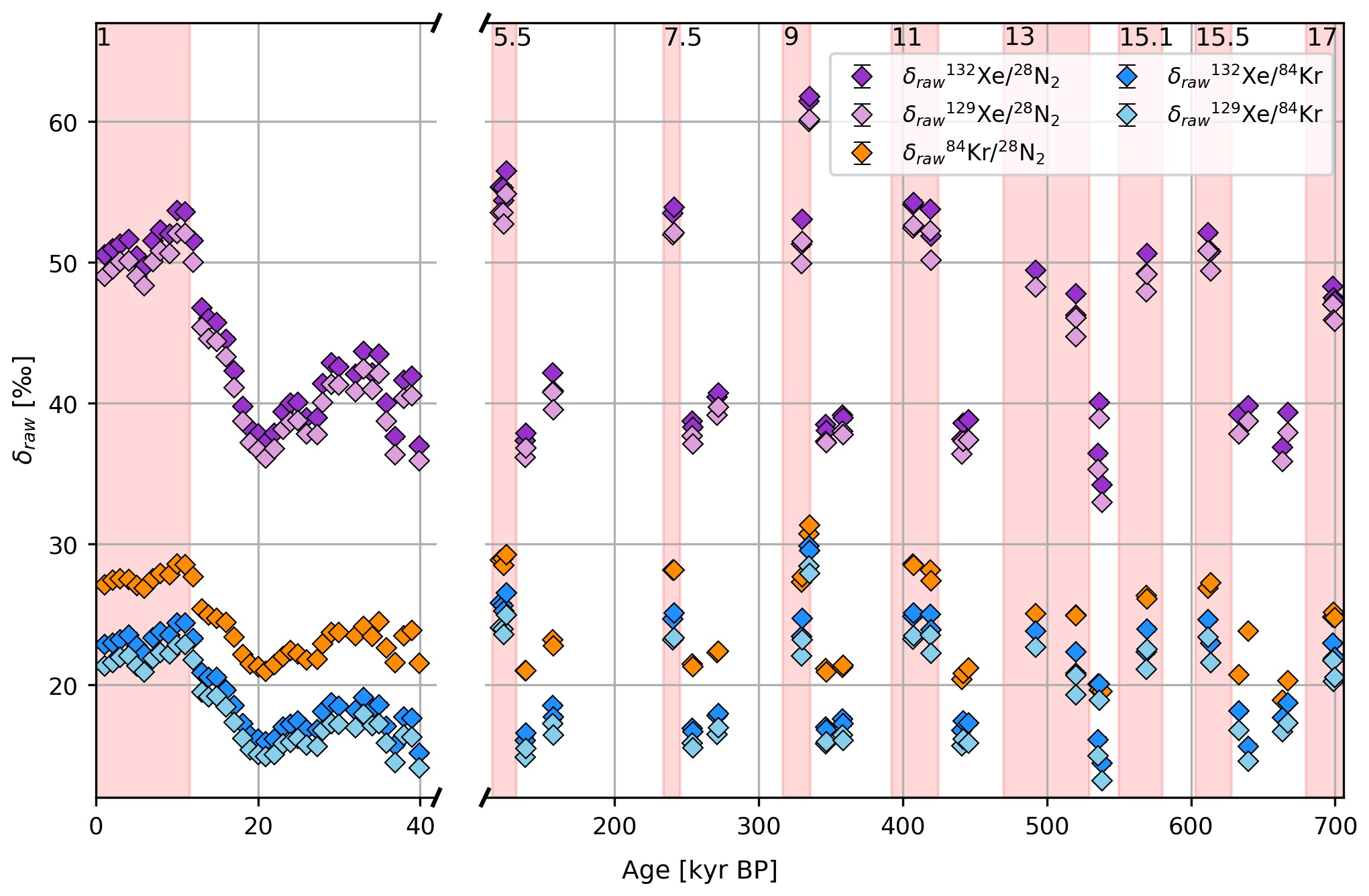
Figure 1Measured delta values of the EDC elemental ratios from 700 kyr BP to the present. The analytical uncertainties of the elemental ratios are too small (on the order of 0.1‰; see text) to be displayed here. The red shaded intervals indicate interglacials as identified by Masson-Delmotte et al. (2010).
2.2 Inferring atmospheric noble gas ratios from raw data
While the troposphere is well-mixed through turbulent processes, the low permeability of the firn restricts bulk flow; thus, the gas transport is controlled by molecular diffusion. All measured isotope and elemental ratios we extract from the ice core samples (reported as “raw ratios”) are therefore highly fractionated with respect to the atmospheric values (as illustrated by the strongly positive δ values in Fig. 1), mainly due to gravitational enrichment in the diffusive zone of the firn but also thermal diffusion if a temperature gradient is present in the firn column (Schwander et al., 1988) or non-diffusive transport processes that disturb the diffusive equilibrium (so-called kinetic fractionation). These systematic fractionations in the isotopic and elemental ratios have to be corrected for, as illustrated in Fig. 2.
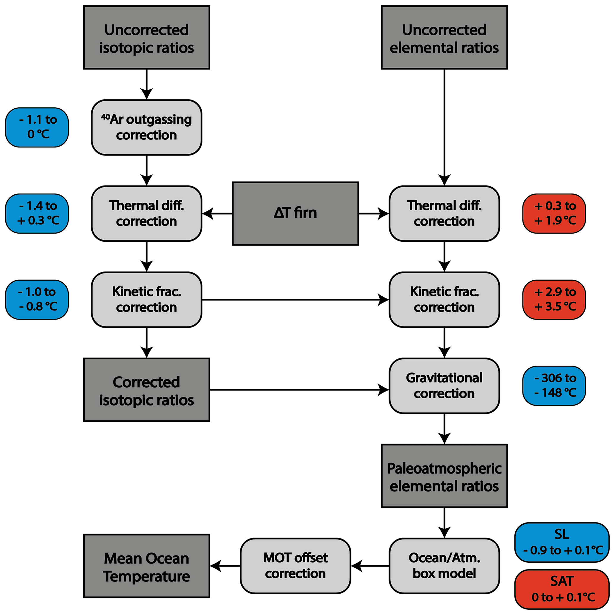
Figure 2Flow scheme to infer paleo-atmospheric elemental ratios and finally MOT using the measured elemental (, , and ) and isotopic ratios (, , ). Values are indicated by dark grey square boxes, while applied corrections are illustrated by rounded boxes in lighter grey. In a first step, the isotope ratios have to be corrected for changes in 40Ar due to geological outgassing. The isotopic and elemental ratios are then corrected for thermal diffusion and kinetic fractionation. The temperature difference between the top and the bottom of the diffusive column height required for the correction of thermal diffusion is derived using either a firn column model (Michel, 2016) or the full matrix of noble gas isotopes. For the kinetic fractionation, we assume fixed ratios between isotopic and elemental ratios (Birner et al., 2018). Finally, the corrected isotopic ratios are used to correct the elemental ratios for the gravitational enrichment. The corrected elemental ratios are then translated into MOT using an ocean atmosphere box model. Here, we correct for the influences of sea level (SL) change and the saturation state (SAT) of the global ocean. In a last step, the resulting MOTs are corrected for their Holocene offset (see text for details). The approximate range of the respective correction performed on all our samples for MOT values can be found in the colored boxes. Positive values (red boxes) imply that the correction leads to an increase in absolute MOT values. It is important to stress that the size of the correction is not a measure of the uncertainty associated with it. The gravitational enrichment correction, for example, dominates all other corrections by orders of magnitude. Nonetheless, the analytical uncertainty of that correction is only minor, as it is largely given by the uncertainty in diffusive column height, the exact determination of which is one of our analytical foci. Also note that it is the size of the range of a correction, rather than the absolute value of the correction, that has an influence on glacial–interglacial MOT differences. For example, although the correction of elemental ratios for kinetic fractionation appears to be the second most influential correction, when considering its absolute value, its range is only narrow. Thus, it alters the glacial–interglacial MOT difference only slightly.
Moreover, post-coring gas losses accompanied by gas fractionation processes have been observed in our samples in the bubble–clathrate transition zone (BCTZ) and in poorly preserved and cracked ice, mainly in the deepest section of the ice core. While the gas fractionation processes mentioned above can be corrected for using the full matrix of noble gases and their isotopes, the gas loss fractionation cannot yet be quantitatively corrected for, and affected samples have to be unambiguously identified using clear detection criteria and removed from the data set. In the following sections, the systematic correction of the isotopic and elemental ratios is described, while the post-coring gas loss and its detection are described in Sect. 3.
2.2.1 Systematic processes altering the isotopic and elemental ratios
Geological outgassing of 40Ar
In contrast to the nitrogen, krypton, and xenon isotopes as well as 36Ar and 38Ar, the atmospheric abundance of 40Ar has gradually increased over time. This atmospheric 40Ar increase is caused by integrated 40Ar outgassing throughout Earth's history due to the radioactive decay of 40K in the crust and mantle (Bender et al., 2008). Assuming the 40Ar increase is constant in time, the effect can be corrected if the age of the sample is known. In this study, we use values corrected for outgassing according to Bender et al. (2008).
Here, the gas age tgas has units of thousands of years before present (kyr BP). The outgassing effect on MOT is small for samples from the last transition (<0.1 ∘C), but it becomes more important for samples in the deeper and older ice (on the order of 1 ∘C for the oldest samples).
Gravitational enrichment
Gas transport in the pore space of the firn column is controlled by molecular diffusion below a convective zone in the top meters of the firn. In this diffusive column molecules of different masses are separated, leading to gravitational enrichment of the heavier gases and isotopes at the bottom of the firn column where bubble close-off occurs. Thus, all elemental and isotopic ratios are strongly enriched in the heavier gases compared to the atmosphere according to
where g is the local gravitational acceleration, R the gas constant, and T the mean firn temperature (Craig et al., 1988; Schwander, 1996). To correct for the gravitational enrichment of the elemental ratios at the lock-in depth, we have to know the diffusive column height (DCH) z of the firn (where z is defined positive downward), which can be directly derived from the isotopic enrichment of the individual gas species after corrections for thermal diffusion and kinetic effects (see below).
Thermal diffusion
The second diffusive process leading to fractionation of the air in the firn column is thermal diffusion. It refers to the fractionation of a gas mixture in the presence of a temperature gradient. This leads to an enrichment of the heavier components at the cold end of the firn column according to the laboratory-determined thermal diffusion sensitivity ΩX/Y for two gas or isotope species X and Y, where ΩX/Y is specific for the gas mixture (Severinghaus et al., 2003).
Here, ΔT is defined as the temperature difference between the top and the bottom of the DCH. As EPICA Dome C is a low-accumulation site, the mean annual firn temperature increases with depth (in the absence of temporal climate changes at the surface; Ritz et al., 1982) due to the geothermal heat flux at the bottom, and the gas enclosed in bubbles is expected to be slightly depleted by thermal diffusion relative to its gravitational value. Note that this thermal fractionation is gas-species-dependent and much larger for the lighter gases. Here we use the thermal diffusion sensitivities given by Kawamura et al. (2013) and Headly (2008).
Kinetic fractionation: the heavy isotope deficit
If only diffusive processes occurred in the firn column, the differences between any of the measured isotope ratios could be used to unambiguously reconstruct the thermal and gravitational fractionation components using the well-known thermal diffusion sensitivity parameters (Kawamura et al., 2013; Headly, 2008). In particular, as the gravitational enrichment of two gases only differs according to the mass difference between two gases, the gravitational enrichment normalized to unit mass difference should be the same for all gases. However, even after the thermal diffusion correction the isotopic ratios of different gases per unit mass difference still reveal systematic offsets (see Fig. 3a), indicating that there is another mechanism at play that we have yet to correct for.
The reason for the systematic differences in the isotopic ratios per unit mass difference between the different gases at Dome C in Fig. 3 is the occurrence of advective processes in the firn such as turbulent mixing at the surface (Kawamura et al., 2013), barometric pumping, and the net vertical movement of air by ice flow and compression (Buizert and Severinghaus, 2016; Birner et al., 2018) that all disturb the diffusive equilibrium in the firn column. The term coined for this difference in measured isotopic ratios per unit mass difference after thermal correction is heavy isotope deficit (HID) (Buizert and Severinghaus, 2016) or differential kinetic fractionation (Birner et al., 2018) between the isotopic or elemental ratio X and another isotopic or elemental ratio Y. Further on, we will use the difference between the kinetic fractionation of an isotopic or elemental ratio X per unit mass difference relative to the kinetic fractionation in N2 isotopes (Kawamura et al., 2013; Birner et al., 2018; Buizert and Severinghaus, 2016). For example, for Ar isotopes this fractionation is defined as
Here, ∗ indicates that the values are normalized to unit mass difference, for example . Note that the heavier (and slowly diffusing) gases like xenon and krypton will be further from diffusive equilibrium than lighter (and faster-diffusing) gases like argon and nitrogen. Another way to put this is that the effective DCH of different gases is not the same, with z being a little shorter for heavier, less diffusive gases.
In our measurements the total deficit of xenon and krypton isotopes relative to argon isotopes per unit mass difference over the last 40 kyr is on average −0.046 ± 0.007 ‰ and −0.029 ± 0.007 ‰, respectively (here and throughout the paper all uncertainties refer to 1σ). This total deficit comes about through the combined effect of different thermal diffusion sensitivities of the different gases and gas-specific kinetic fractionation. Separation of these two effects on the total deficit requires corrections for the thermal gradient, as described in Sect. 2.2.2.
Birner et al. (2018) discovered that while the absolute magnitude of kinetic fractionation may vary substantially between different ice core sites, the kinetic fractionations between two gases occur in fixed ratios between isotopic and elemental ratios for a variety of firn regimes. Thus, although we do not know the absolute kinetic fractionation at Dome C for an individual gas for past firn conditions a priori, we can use the results by Birner et al. (2018) together with our multiple gas species and transient firn temperature modeling to correct for the HID and other gas transport effects. It is worth noting that the ratios of the mean kinetic fractionations over the last 40 kyr as displayed in Fig. 3 agree well within uncertainties with the ratios predicted by Birner et al. (2018). Note that the kinetic fractionations for the last 40 kyr displayed in Fig. 3 also suggest, apart from substantial analytical scatter, some systematic variations. As these systematic variations are generally in line with the fractionation ratios predicted by Birner et al. (2018), the changes are likely caused by changing kinetic fractionation conditions with time (stronger barometric pumping, higher wind speeds at the surface, etc.). However, some samples older than 40 kyr show much higher deviations from the mean that cannot be explained by analytical uncertainty or changing kinetic fractionation. Accordingly, we do not use the individual HID values of each sample as displayed in Fig. 3b for samples older than 40 kyr to quantify . Instead, we use the mean isotopic fractionation derived for the last 40 kyr and assume that this mean value is also representative for the correction of our samples older than 40 kyr. As the choice of has a systematic effect on the final reconstructed MOT, we also take the variation of over the last 40 kyr into account to quantify the systematic uncertainty introduced by this choice. Thus, we use the mean kinetic fractionation over the last 40 kyr plus (minus) its standard deviation as upper (lower) bounds of the kinetic fraction to calculate MOT. We regard this as a systematic uncertainty in our MOT reconstruction and separate this uncertainty from the stochastic uncertainty introduced by the analytical error.
Gas loss effects on isotopic ratios
As mentioned in the previous paragraph, ice core samples with heavy post-coring gas loss exhibit enriched , while δ15N is unaffected (J. Severinghaus, personal communication, 2021). Due to their large size, the krypton and xenon isotopes are also not affected. Correction coefficients for argon isotope enrichment in bubble ice have been suggested by Kobashi et al. (2008b), but it is not certain whether these correction factors describe the gas loss quantitatively and in particular whether they can be used for ice from any depth and for all ice cores. We refrain from trying to correct this effect because we do not see evidence for an isotope fractionating effect by artifactual gas loss (see Sect. 3.1) and because no correction coefficients have been established for clathrate ice.
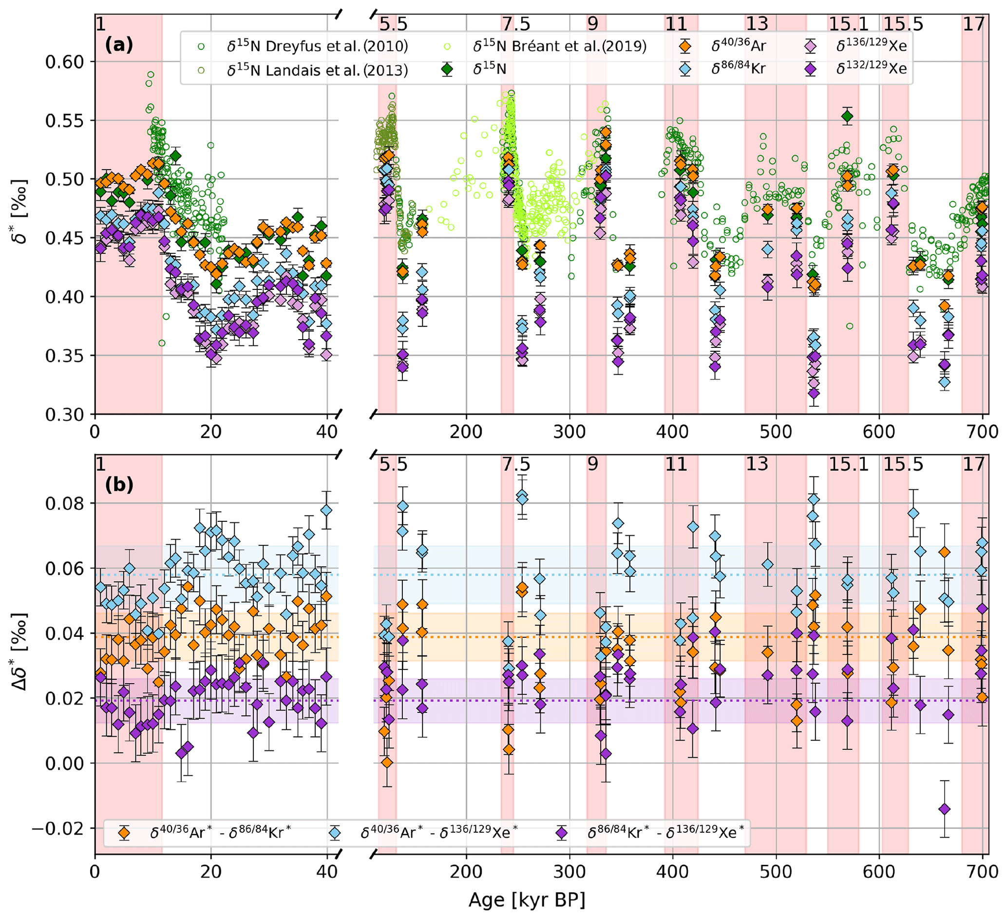
Figure 3(a) Isotopic enrichment of the EDC samples from 700 kyr BP to the present. All isotopic data are shown per unit mass difference and reported relative to modern air sampled in Bern, Switzerland. The data are corrected for thermal fractionation as described in the text. In the case of δ15N, data points contaminated with drilling fluid have been excluded. The circles in darker green, olive, and lighter green represent measurements from the EDC ice core from Dreyfus et al. (2010), Landais et al. (2013), and Bréant et al. (2019), which have been corrected for thermal fractionation using our model-derived firn temperatures. (b) Difference between the isotopic ratios of the EDC samples after correction for thermal fractionation. The dashed line is the mean difference from the samples over the last 40 kyr, with the shaded areas representing their standard deviation. The red shaded intervals and the MIS numbers on top indicate interglacials as identified by Masson-Delmotte et al. (2010).
2.2.2 Correcting isotopic ratios for transport processes in the firn column
As outlined above, the measured isotopic ratio is influenced by a series of processes that alter the paleo-atmospheric value . We can write the following for the measured isotopic ratio.
Note that we assume ocean solubility effects on the isotopic ratios to be negligible (in contrast to the elemental ratios, for which we use these effects to quantify MOT). This can be justified using a two-box model calculation with the recently determined solubility fractionation factors in seawater (Seltzer et al., 2019) and imposed ocean temperature differences, which yields glacial–interglacial changes in atmospheric noble gas isotope composition of less than 0.001 ‰ per unit mass difference. We can thus safely assume that for isotopic ratios (where for Ar isotopes the atmospheric value has to be corrected for Ar outgassing as described in Sect. 2.2.2).
Using the measured isotopic ratios we are able to quantify the fractionation effects and correct the isotopic and elemental ratios. Here we explore two different correction pathways that differ in the derivation of ΔT, which is required to quantify the thermal diffusion effect. Both possibilities use the matrix of isotopic ratios to constrain the gravitational enrichment and the HID. However, one possibility uses a 1D ice flow model connected to a dynamic heat advection and diffusion model (Michel, 2016) to quantify the thermal diffusion effect, while the other uses the full matrix of noble gas isotopes measured in this study to quantify ΔT empirically.
(a) Correction using a firn temperature model
To correct for the strong gravitational enrichment (large mass difference) we can use the precisely measured isotopic ratios after correcting for thermal diffusion and kinetic fractionation. Due to the firn temperature slightly increasing with depth at EDC and due to the negative kinetic fractionation for heavier gases, the corrected isotopic ratios are slightly increased compared to the measured ratio. The results for the thermally corrected isotopic ratios reflecting the remnant kinetic fractionation are shown in Fig. 3a, where ΔT used for the thermal correction of each individual sample was calculated using an ice flow–heat flow model as described below. The isotopic ratio least affected by kinetic fractionation is δ15N; however, our δ15N measurements are not as precise as per unit mass difference, and some of the δ15N values had to be discarded due to drill fluid contamination affecting the mass spectrometric analysis. Accordingly, we use as our reference isotope. In many applications to reconstruct temperature using isotopic ratios of permanent gases (e.g., Kobashi et al., 2008a), the small kinetic fraction of Ar relative to N2 is neglected and the gravitational enrichment per unit mass difference in units of per mill is calculated according to
where the ∗ in indicates that the thermal sensitivity has been normalized to unit mass difference.
However, firn gas pumping and modeling experiments (Kawamura et al., 2013) show that all gases are subject to kinetic fractionation, and therefore even Ar isotopes show a small heavy isotope deficit after correction of thermal diffusion effects (Buizert and Severinghaus, 2016) compared to nitrogen isotopes. Thus, should be calculated according to
The absolute kinetic fractionation in Eq. (7) is not known a priori and is dependent on firn and meteorological conditions at the site that may have changed in the past. Using the equivalent equation for Xe isotopes and the linear relationship of the kinetic fractionations given by Birner et al. (2018), can be calculated from our measurements according to
Note that while including the kinetic fractionation may improve the accuracy of the reconstruction, it slightly decreases the precision, as the analytical error for Xe isotopes also comes into play.
ΔT in Eqs. (7) and (8) is unknown but can be estimated for each individual sample using an ice flow–heat flow model that solves the ice advection–firn compaction and the heat advection and diffusion equation transiently over the last million years. Here we used the model by Michel (2016) and a parameterization of heat diffusion and heat conductivity according to Cuffey and Paterson (2010). The density of the firn was estimated by the Herron–Langway model (Michel, 2016). Heat diffusivity of the very porous top 10 m of the firn was corrected according to Weller and Schwerdtfeger (1970). The recent firn temperature difference ΔT in this run agreed within ±0.2 ∘C between the model and measured firn temperature profiles at Dome C (Buizert et al., 2020). We assume that ±0.2∘C represents the analytical uncertainty of the model. Surface temperature and snow accumulation used in the model are prescribed using the EDC temperature record over the last 800 000 years (Jouzel et al., 2007; Bazin et al., 2013), and a scaled version of the stacked marine δ18O record (Lisiecki and Raymo, 2005) is used for earlier times. For an optimal fit with the measured temperature profile over the entire ice thickness at Dome C, a +2 ∘C correction of glacial temperatures was applied by Michel (2016); however, this has only a very small effect on the firn temperature difference. Ice thickness changes over the last 800 kyr are taken from Parrenin et al. (2007), and a scaled version of the stacked marine δ18O record is used for earlier times. The constant geothermal heat flux and the thinning function were chosen to optimize the agreement of the modeled temperature profile with borehole temperature measurements (Buizert et al., 2020) and the age profile at Dome C (Bazin et al., 2013).
The DCH affects both the gravitational enrichment and the absolute value of the temperature gradient. Accordingly, we use an iterative approach for Eq. (7) to determine the firn temperature gradient from the model results. In the first step we neglect the temperature gradient, and thus thermodiffusion effects, to estimate the DCH:
where Δm∗ is the unit mass difference in kilograms per mole (kg mol−1). After this first step we read out the modeled firn temperature difference for this depth and use it for the thermal diffusion correction in the next step. Using this iterative approach the firn column depth converges after two iterations. This model-based analysis shows that the firn column depth is about 70–80 m for glacial periods and 90–100 m for interglacials.
The kinetic fractionation calculated using modeled ΔT is on average ‰ (1σ) over the last 40 kyr (note that the HID values given in Fig. 3b represent a measure of scaled by a factor of 6.3, 4.25, and 2.05 for , , and , respectively, as derived from Birner et al., 2018). As described above, we use the mean plus or minus the standard deviation of the kinetic fractionation over the last 40 kyr to also correct the samples older than 40 kyr and to assess the uncertainty introduced by this correction.
The last unknown in Eqs. (7) and (4) is the amount of kinetic fractionation for nitrogen isotopes . Modeling and firn air studies by Buizert and Severinghaus (2016) and Birner et al. (2018) show that at WAIS Divide, i.e., a site on the West Antarctic Plateau, this fractionation is less than 0.005 ‰, while at Law Dome, a site subject to strong barometric pumping, it may be larger (J. Severinghaus, personal communication, 2021). Assuming a kinetic fractionation at Dome C that is similar to WAIS, this small fractionation in translates into an offset in the final MOT values on the order of 0.01 ∘C and can therefore be safely neglected in our MOT reconstruction.
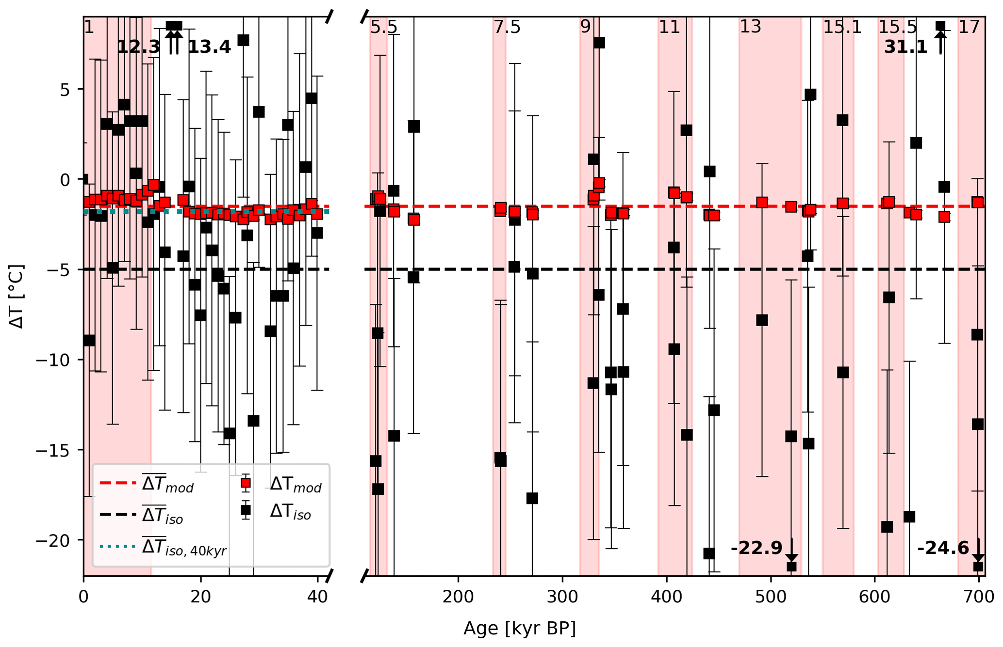
Figure 4Comparison of the firn temperature difference ΔTmod, as derived from the ice flow–heat flow model of Michel (2016) (red squares), and ΔTiso obtained using measured isotopic ratios only (black squares). Dashed lines in red and black indicate the overall mean values for ΔTmod and ΔTiso, while the dotted line in cyan represents the mean ΔTiso when considering samples from the first 40 kyr only. The red shaded intervals and the MIS numbers on top indicate interglacials as identified by Masson-Delmotte et al. (2010).
In the following, we assume for Dome C, where synoptic pressure variations and wind speeds are rather low. Neglecting potential errors in the thermal diffusion sensitivities, the uncertainty in introduced by this model-based method to correct the data is 0.003 ‰ (1σ).
(b) Correction using measured isotopic ratios only
Using the firn temperature model as in (a) assumes that the firn temperature difference in the model over the DCH realistically resembles the temperature difference seen by the gas at the age of each individual sample. The model neglects, for example, seasonal variations in the temperature gradient, which may not cancel out in the long-term annual average, and also assumes that the current parameterizations used for firn density, heat conduction, and heat diffusivity profiles in the firn are also representative for past conditions. An alternative way is therefore to use only experimental evidence from our full matrix of isotope ratios. Assuming that gravitational enrichment, thermal diffusion, and kinetic fractionation completely describe the fractionation processes occurring in the firn column, this approach provides a purely measurement-based estimate of and ΔT.
The equivalent to Eq. (8) for Kr isotopes is
with the constant ratio of kinetic fractionations for different isotopes given by Birner et al. (2018).
Solving Eq. (8) for ΔT and inserting it into Eq. (10), it follows that
where . Note that the mean kinetic fractionation derived using this data-based approach is on average −0.009 ‰ over the last 40 kyr and thus in perfect agreement with the results from the firn temperature model approach.
Using Eq. (11) in Eq. (8) finally leads to
While this method in principle avoids any potential systematic uncertainties in the firn temperature gradient, it substantially increases the uncertainty of the reconstruction, as now the analytical uncertainties of all three noble gas isotopic ratios have to be taken into account for each individual sample. Using Monte Carlo error propagation, the uncertainty in derived in this approach is increased to 0.01 ‰ (i.e., roughly 10 times larger than in the model-based approach), and the uncertainty in ΔT becomes about 8 ∘C. This translates into an error for of roughly 0.08 ‰ (i.e., almost 30 times higher than in the model-based approach) and finally into an error in the corrected elemental ratios (see Sect. 2.2.3) of several per mill, which is prohibitive for a reliable reconstruction of MOT for individual samples.
The very high scatter in data-derived ΔT is displayed in Fig. 4. The standard deviation of ΔT over the last 40 kyr is 6 ∘C, which is of the same order as the expected analytical uncertainty in ΔT of 8 ∘C derived from error propagation. Hence, this large scatter can be explained by analytical noise and shows that any systematic variation in ΔT over the last 40 kyr cannot be reliably quantified using the data-based approach.
Looking at Fig. 4 it should be stressed that despite the large scatter the mean ΔT over the last 40 kyr derived in this data-based approach is in excellent agreement with ΔT derived in the model-based approach. This points to the fact that using our noble gas isotope measurements we are able to accurately (but not sufficiently precisely) reconstruct and ΔT over the last 40 kyr and that thermal diffusion and kinetic fractionation fully explain the systematic offsets of the isotopic ratios.
However, for the samples older than 40 kyr the average ΔT is ∘C, which is physically not in line with the observed or modeled firn temperature differences and also not in line with the results younger than 40 kyr. As we do not expect that any unknown firn fractionation processes were active prior to 40 kyr BP that did not occur over the last 40 kyr, this apparent offset in ΔT either reflects the large scatter of the data or is related to an isotope fractionating Ar loss process during transport, when the samples got relatively warm for a short period of time.
As mentioned above, using the data-based approach to correct the elemental ratios for each individual sample is not a viable solution, as the scatter in reconstructed ΔT, , and thus MOT is too large. Therefore, we regard the mean and ΔT values over the last 40 kyr to be representative for the entire record and use those to calculate . To quantify the systematic uncertainty introduced by this choice of and ΔT, we calculate an upper (lower) estimate of ΔT and as defined by their mean values over the last 40 kyr plus (minus) their standard deviation. This provides us with a range of values for for the systematic corrections of the elemental ratios (see Sect. 2.2.3). We refer to this correction as the mean data-based approach further on.
We stress that while such a constant correction with a systematic range of possible values has a significant impact on the absolute reconstructed MOT value, the impact of the correction on the glacial–interglacial difference in MOT is small. Moreover, the glacial–interglacial difference in MOT is very similar whether one uses the model-based approach in (a) or the mean data-based approach in (b). Accordingly, only MOT differences relative to the Holocene are considered, as was also the case in the study by Shackleton et al. (2020).
In summary, the data-based approach shows that we can quantitatively correct the gas-transport-related fractionations that occur in the firn column; however, the precision of the data-based approach is not sufficient for single samples. Accordingly, in the discussion of our final MOT data in Sect. 4 we do not use the data-based approach and rely on the much more precise model-based correction.
2.2.3 Correction of the elemental ratios
Equivalent to isotopic ratios of one gas species, the ratios of two different gas species (here referred to as elemental ratios) have to be corrected for gravitational enrichment. Due to the large mass difference between two gas species, this gravitational correction of elemental ratios is substantial. In addition, thermal diffusion and kinetic fractionation have to be corrected in the elemental ratios. For the ratio this can be summarized according to
where again we set , as the effect of is negligible compared to other uncertainties. The first factor in brackets on the right-hand side represents the measured value of the elemental ratio corrected for thermal diffusion and kinetic fractionation, while the second factor corrects this isotopic ratio for its gravitational enrichment. ΔT, , and can be calculated from the firn temperature model and from the isotopic data as described above using the fixed ratios of kinetic fractionation given by Birner et al. (2018). Note that the exponent is very large (e.g., 56 for 84Kr and 28N2); thus, the gravitational correction is substantial and sensitive to any analytical error in the isotopic ratios as well as in uncertainties in the thermal correction and the kinetic fractionation.
Here we use both the model-based and the mean data-based reconstruction of ΔT and described above and apply these to Eq. (13) and equivalent equations for and ratios. The results of these corrections are shown in panel (a) (model-based reconstruction) and (b) (mean data-based reconstruction) of Fig. 5. Note that the whiskers in Fig. 5 represent the stochastic error (1σ) due to error propagation of the analytical uncertainties, while the size of the boxes represents the systematic uncertainties (1σ) introduced by our choice of mean ΔT and .
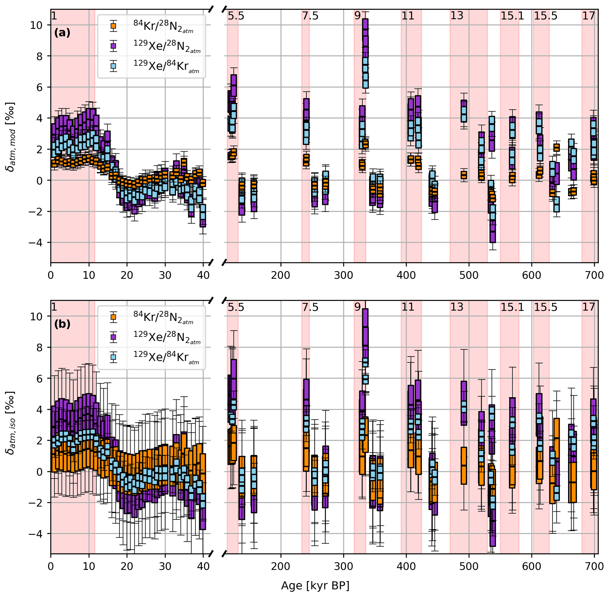
Figure 5Comparison of the reconstructed atmospheric ratios of (orange), (purple), and (blue) (a) as derived from the calibrated firn model of Michel (2016) (b) using measured isotopic ratios only. The reconstructed value is drawn as a black line in the middle of each box. The magnitude of the systematic uncertainty is indicated by the size of the colored boxes, and the statistical uncertainties are depicted as whiskers (1σ each). The red shaded intervals and the MIS numbers on top indicate interglacials as identified by Masson-Delmotte et al. (2010).
The first observation is that the three different atmospheric elemental ratios have different glacial–interglacial amplitudes, primarily reflecting the different temperature sensitivities of gas solubility in the ocean as expected. Secondly, the corrected elemental ratios show that although our data are referenced to recent outside air at Bern, reflecting late Holocene ocean temperatures, the Holocene elemental ratios after all corrections are not equal to zero but systematically shifted to positive values.
Holocene elemental ratios larger than zero have also been recently observed by Shackleton et al. (2020) using Taylor Glacier ice, reflecting our insufficient quantitative understanding of fractionation processes in the firn; this requires more dedicated firn gas sampling and firn gas transport modeling studies that realistically resolve seasonal variations in the gas transport, pressure variability, and kinetic fractionation. However, glacial–interglacial differences in our corrected elemental ratios are not sensitive to this overall offset. If we use changes in atmospheric elemental ratios relative to the Holocene mean, both the model-based and the mean data-based approach provide very similar results. For example, using the model-based approach, the corrected last glacial values are on average about 3.0 ‰ lower than the Holocene values, which is in agreement within uncertainties with the results by Bereiter et al. (2018b) using ice from the WAIS Divide ice core.
The final observation pertains to the scatter of the data. Elemental ratios corrected using ΔT and derived using the data-based approach for each individual sample provide no meaningful results, as the analytical scatter introduced from all three isotopic ratios is too large.
Using the model-based approach, we introduce uncertainty through the elemental ratio analysis, the uncertainty in our model-based ΔT, and systematic uncertainty through our use of the mean over the last 40 kyr to correct the kinetic fractionation. This leads to a substantially smaller scatter than in the individual data-based approach. The stochastic errors (1σ) in δKr / N2,atm, δXe / N2,atm, and δXe / Kratm introduced by the measurement errors are 0.20 ‰, 0.45 ‰, and 0.32 ‰, respectively, in our model-based approach. The systematic uncertainty in this case is 0.23 ‰, 0.70 ‰, and 0.48 ‰, respectively.
Alternatively, we can use the mean data-based correction approach. Using the mean ΔT and over the last 40 kyr leads to the smallest scatter in our atmospheric elemental ratios, as we average over 39 data points for our correction. However, this also implies a large systematic uncertainty that derives from the choice of mean ΔT and . Moreover, both parameters may have been subject to systematic changes over time that we cannot decipher using this mean correction. The stochastic errors (1σ) in δKr / N2,atm, δXe / N2,atm, and δXe / Kratm introduced by the measurement errors are 1.68 ‰, 2.12 ‰, and 0.66 ‰, respectively, in our mean data-based approach. The systematic uncertainty in this case is on average 1.22 ‰, 1.49 ‰, and 0.40 ‰, respectively.
In summary, our different correction pathways lead to similar results in the differences of atmospheric elemental ratios relative to their Holocene value. In the following, we will use only the atmospheric elemental ratios after correction using the model-based approach, which is based on well-understood physical laws of heat conduction–advection and provides elemental ratios with sufficient precision and accuracy to reconstruct glacial–interglacial changes in MOT after correction for gravitational, thermal, and kinetic fractionation.
2.3 Box model to infer the MOT from atmospheric values
To reconstruct MOT values from the corrected elemental ratios, we use the ocean–atmosphere box model described by Bereiter et al. (2018b), except for one slight update, as we use the solubility equations given by Jenkins et al. (2019). The basic assumption in the model is that N2, Kr, and Xe are conserved in the ocean–atmosphere system and that their distribution between the two reservoirs is controlled by the temperature-dependent dissolution in the ocean water. The model accounts for the effects of changes in ocean salinity, volume, and atmospheric pressure on the oceanic inventories of each of the three gases, which have individual temperature-dependent solubilities. The records of Lambeck et al. (2014) and Spratt and Lisiecki (2016) are used to reconstruct the sea level for the last 27 kyr and the time interval 28–800 kyr BP, respectively. We assume a constant undersaturation of the heavy noble gases in the ocean by 3 % for Xe and 1.5 % for Kr (Hamme and Severinghaus, 2007; Loose et al., 2016; Hamme et al., 2019). In contrast to Bereiter et al. (2018b) we do not impose a temporal change in this undersaturation, as we have no observational evidence about such a change in saturation state and we cannot provide a convincing argument on whether the saturation may have increased or decreased during glacial times. The overall slower ocean overturn in the glacial may suggest an increase in saturation, while the expansion of sea ice (especially in the Southern Ocean) would speak for a stronger undersaturation of the heavy noble gases. Accordingly, we refrain from changing the saturation state in our model. Sensitivity analyses show that a reduction of the glacial undersaturation to half its current value will lead to a warming of our glacial MOT reconstruction by a few tens of a degree.
Using this box model we can translate the reconstructed and corrected atmospheric elemental ratios (, , and ) into changes in MOT relative to the Holocene. Using our model-based correction approach described above leads to an MOT change over the last glacial–interglacial transition of on average 3.0 ± 0.4 ∘C, 3.3 ± 0.4 ∘C, and 3.6 ± 0.4 ∘C for δKr N2,atm, δXe N2,atm, and atm, respectively (see Fig. 6 and Table 2). This is in general agreement within uncertainties with independently derived results over the last glacial termination for the WAIS Divide ice core from Bereiter et al. (2018a).
Table 2Absolute MOT anomaly based on in degrees Celsius (∘C) relative to the Holocene mean using both of our correction approaches. The Holocene value is the average of 10 EDC samples from 0–10.0 kyr BP, the LGM value is the average of nine samples between 17.8 and 26 kyr BP, LIG is the average of four samples between 120 and 129.9 kyr BP, and MIS 6 includes four samples from 135–160 kyr BP. MIS 9 and MIS 10 each comprise four samples.
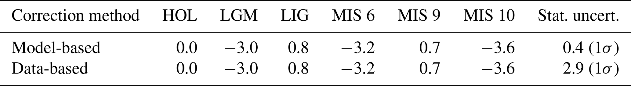
As described above, the uncertainties in the model-based correction approach for elemental ratios are introduced by uncertainties in the modeled ΔT, the measurement errors of the elemental ratios, and the choice of . For the Ar isotopes we also corrected for the steady increase in 40Ar through the decay of 40K in the crust and mantle, which leads to a small long-term increase in . This increase was experimentally determined by Bender et al. (2008) and has a slope of 0.066 ± 0.007 ‰ per million years, which we include in our error propagation. Moreover, the box model approach may add some minor systematic uncertainty, which we cannot quantify. Using the analytical uncertainties in the elemental ratios in the model-based approach leads to a stochastic uncertainty (1σ) in the MOT values between 0.35 and 0.41 ∘C for all three elemental ratios and a systematic uncertainty of 0.38–0.51 ∘C.
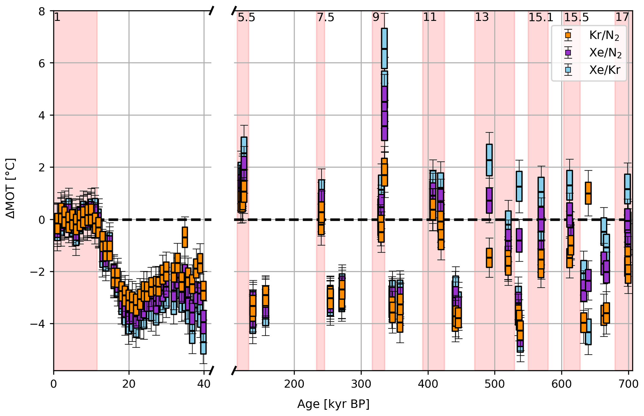
Figure 6Reconstructed MOT for the EDC samples over the last 700 kyr relative to the Holocene value (using the model-based correction). MOTs are derived from (orange), (purple), and (blue). The horizontal line in the middle of the filled box provides the corrected value. The boundaries of the filled boxes refer to the systematic uncertainty, while whiskers reflect the stochastic uncertainty introduced by the measurement errors (each 1σ). The red shaded intervals and the MIS numbers on top indicate interglacials as identified by Masson-Delmotte et al. (2010).
Additional changes in the elemental ratios may occur if post-coring gas loss leads to fractionation between different gases. While visible cracks are avoided in the sample preparation, previous ice core studies showed that invisible microcracks can occur, leading to gas loss fractionation processes that affect, for example, and , but little is known about gas loss effects on heavy noble gas ratios. Ice subject to such internal microcracks is most susceptible to post-coring gas loss, and accordingly we find systematic deviations in the MOT values derived from the three different elemental ratios in (i) ice from the bubble–clathrate transition zone (BCTZ), which is characterized by brittle ice, and (ii) in the oldest, bottommost meteoric ice of the EDC core, which is characterized by particularly large ice crystals and high in situ temperatures and which is prone to increased microfracturing. The following sections address potential gas loss fractionations in these ice zones.
3.1 Post-coring gas loss effects in the BCTZ
Post-coring fractionation of elemental gas ratios is caused by the selective loss of specific gases in poorly preserved samples or in samples from the bubble–clathrate transition zone (BCTZ), i.e., the depth section between the formation of the first clathrate and the disappearance of the last bubble (Lipenkov, 2000).
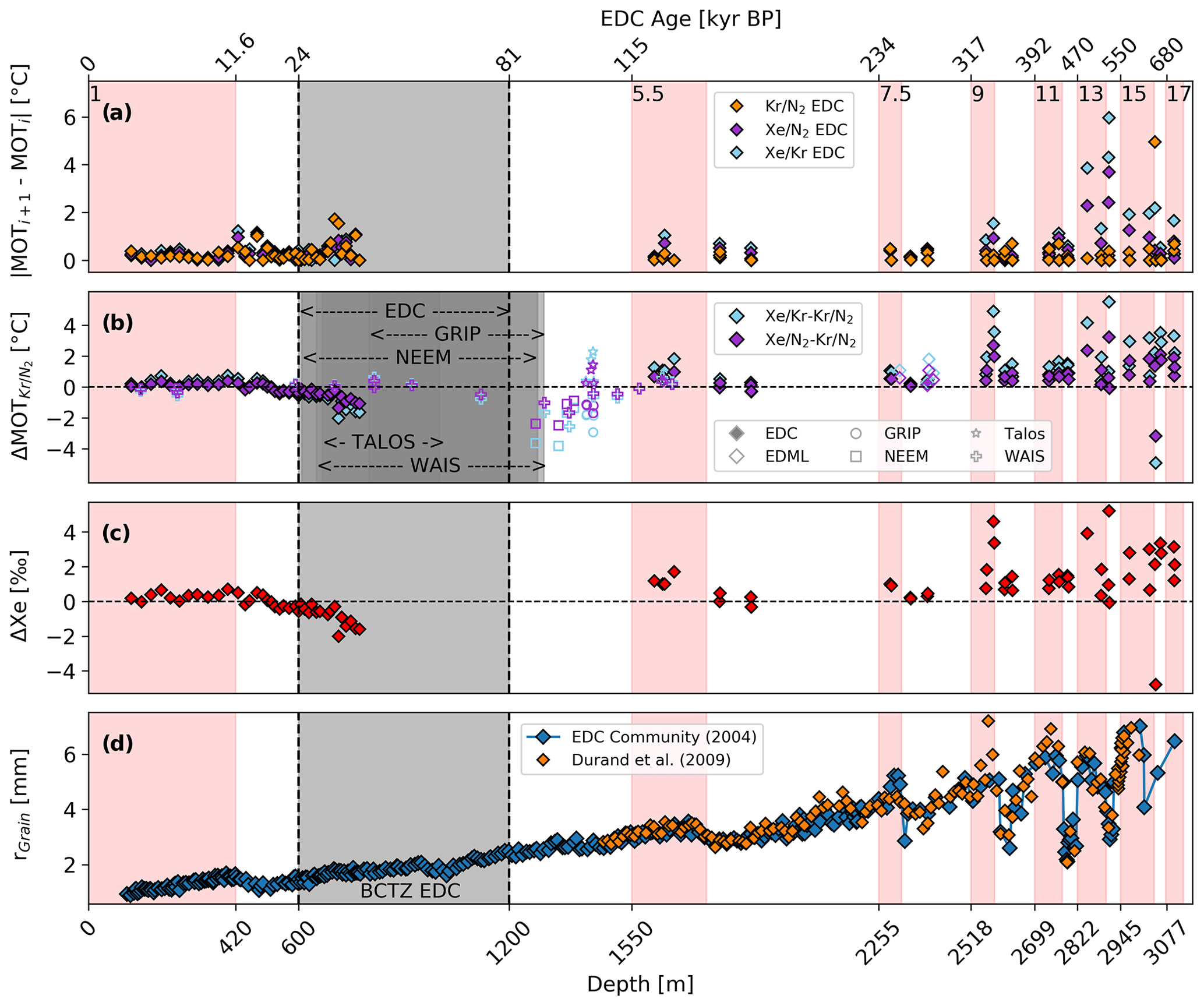
Figure 7(a) Absolute MOT pair difference between two adjacent samples for the three different atmospheric noble gas ratios. (b) Difference in the MOT from and compared to . EDC, GRIP, NEEM, and Talos samples were measured at the University of Bern. WAIS samples were measured by Bereiter et al. (2018b). The grey shaded bars and arrows indicate the BCTZ for the different cores as identified by Neff (2014). All data are corrected for gravitational and thermal fractionation using argon isotopes. EDC samples are also corrected for HID fractionation. (c) Potential xenon change required for the EDC samples to match the MOTs using a least square approach. Given in red is the potential xenon change that minimizes the difference between the MOTs derived from , , and . Negative values indicate a xenon loss, i.e., a depletion of the raw elemental ratios and caused by post-coring gas loss. Positive values represent apparent net xenon “gains” due to higher losses of krypton and nitrogen compared to xenon. (d) Evolution of the grain radius in the EDC core (EPICA community members, 2004; Durand et al., 2009). Note that the ages provided on the upper x axis only apply for samples from the EDC ice core. MIS interglacials (red shaded intervals) as identified by Masson-Delmotte et al. (2010) are labeled at the top for orientation.
Bender (2002) called such gas loss through cracks or microcracks “core-cracking fractionation” and observed this effect to strongly affect in the BCTZ of the Vostok ice core. The effect is explained by gas fractionation occurring between coexisting bubbles and clathrates in combination with post-coring gas loss. In our record we observe small but linearly increasing differences with age (and depth) in the MOT derived from the different noble gas combinations in ice at the top of the BCTZ, i.e., in the zone where clathrates form (600–775 m; 24–40 kyr BP). In particular, MOTs derived from show higher temperatures compared to and in this ice, while the three values agree within their uncertainties in pure bubble ice. Similar systematic offsets are observed around the BCTZ in cores from various sites (GRIP, NEEM, and Talos) but to a variable extent, as shown in Fig. 7b. Bereiter et al. (2018a) also observed pronounced alteration in the trapped gas towards the lower end of the BCTZ or even below for the WAIS ice core.
In the following discussion, we will try to motivate the processes that we think are responsible for this fractionation. Studies of air bubbles and clathrate inclusions on the Dome Fuji ice core provide information on clathrate formation and clathrate growth in cold Antarctic ice (Uchida et al., 2011). Clathrate formation starts when the bubble pressure, which increases linearly with depth due to the increasing hydrostatic pressure, reaches the dissociation pressure of air hydrate. The dissociation pressure of the air hydrate is given by the dissociation pressure of hydrates formed by the pure gas species multiplied by the mole fraction of the gas species in air (Miller 1969). Accordingly, the air hydrate dissociation pressure in the ice is mainly determined by the dissociation pressure of N2 and O2, with minor contributions from Ar or CO2. We assume that any SII-clathrate-forming gas species (Sloan and Koh, 2007) will be quantitatively incorporated into the SII air hydrate structure during its nucleation from an air bubble; however, we speculate that SI-forming gases (such as Xe) may not (or not quantitatively) be incorporated into the SII air hydrate structure in the ice.
As described in Uchida et al. (2011), the number and also the radius of air hydrate crystals increase in the BCTZ at Dome Fuji, which has very similar climatic conditions compared to EDC. This can be interpreted in the BCTZ as more and more hydrates slowly nucleating from bubbles and bubbles and clathrates coexisting for a long time. Due to the higher partial pressures of gas species in bubbles compared to clathrates a constant permeation flux of gas from the bubbles to the clathrates exists, which is the main cause of clathrate growth in the BCTZ at Dome Fuji (or EDC). Note that due to the different permeation constants of different gas species in ice, this transport implies a fractionation of different gas species, which enriches fast-permeating gases (such as O2; Ikeda et al., 2000) in the hydrate and depletes them in the remaining bubble. For Xe we speculate that there is either no permeation flux (if Xe is not included in the SII hydrate structure) or the permeation flux is very small due to the very low permeation coefficient of the large Xe atom. Thus, Xe is depleted in the air hydrate forming in the BCTZ and enriched in the remaining bubbles. After complete collapse of the bubble, we expect the Xe to be “dissolved” in the ice matrix.
Below the BCTZ Uchida et al. (2011) observe an increase in hydrate radius and at the same time a decline in hydrate number. This can be explained by an Ostwald ripening process, leading to the growth of large hydrates at the cost of small ones through the Gibbs–Thomson effect (Uchida et al., 2011). Again, the accompanying gas transport from a small to a large hydrate crystal is supplied by (fractionating) permeation of gas species through the ice. If this process goes on for a sufficiently long time, however, a diffusive re-equilibration of the mole fractions of gas species in the hydrates (such as CO2) is been observed (Lüthi et al., 2010). We assume that this permeation acts on all SII-forming gas species but that SI-forming Xe either does not permeate at all or that the permeation flux is strongly reduced compared to other gas species. Thus, Xe would be depleted in the large clathrates formed by this Ostwald ripening process and would remain dissolved in the ice matrix after complete disappearance of a small clathrate.
We attribute the gradually increasing offsets in reconstructed MOT at the top of the BCTZ to core-cracking gas loss in combination with the fractionation of gases by permeation. Gas enclosed in bubbles is more likely to be lost through cracks after core retrieval than gas in hydrates; thus, if post-coring gas loss from bubbles occurs, the remaining gas of the ice sample will be enriched in O2 relative to N2 and depleted in Xe. The small but significant and decrease in the BCTZ can therefore be explained by the observation that during the gas loss process, Xe is preferentially lost via cracks from the Xe-enriched bubbles.
To quantify a potential Xe loss we use a least squares approach that artificially changes the Xe abundance in the ice to minimize the difference between the three MOT proxies. The respective calculated post-coring Xe loss is shown in Fig. 7c, where the per mill value is the change in the elemental ratio used to minimize the MOT differences compared to . It shows that Xe loss is almost negligible in the top 500 m, i.e., in bubble ice, and increases to about 2 ‰, meaning that the elemental ratio is depleted in Xe by up to 2 ‰ caused by post-coring Xe loss from ice in the BCTZ.
Previous studies have shown that the gas loss effect on is most pronounced when the ice is brittle with an enhanced number of cracks but that the quality of the data is also affected in non-brittle ice if the samples are stored for an extended amount of time at relatively warm temperatures of around −25 ∘C (Ikeda-Fukazawa et al., 2005; Landais et al., 2012). The storage temperature may also affect our noble gas ratio results because our samples from the last transition were stored for about 15 years at about −22 ∘C. The samples from older climatic intervals presented in this study were stored at Dome C and later in Bern in a freezer at a temperature below −50 ∘C. Thus, no gas loss is expected for these samples during storage. However, these samples experienced a short-term warming during transport, when cooling failed during transit. Temperatures were as warm as −16 ∘C at the bottom of the well-insulated transport box and −6 ∘C on top of the box for several hours; however, the ice never reached the melting point.
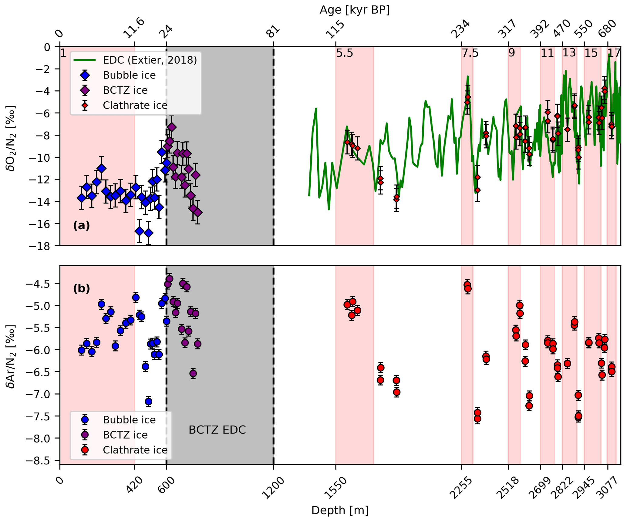
Figure 8Measurements of δ and from the Dome C ice core on the EDC depth scale. The δ record from Extier et al. (2018) is corrected for gravitational enrichment using δ15N2. Our δ data are corrected for gravitational enrichment using , while the data are corrected for gravitational enrichment, thermal diffusion, kinetic fractionation, and geological Ar outgassing. The data show a large variability in the BCTZ and reproducible values for clathrated ice. (a) The green line represents measurements from Extier et al. (2018), and diamonds represent the EDC measurements of δ in this study. (b) EDC measurements of from this study. Interglacial MISs (red shaded areas) as identified by Masson-Delmotte et al. (2010) are labeled for orientation.
To assess the potential loss of gas due to high storage or transport temperature, we compare the that we measure alongside the noble gases with previous measurements on EDC ice stored at −50 ∘C by Extier et al. (2018); the latter did not experience significant warming during transport. Similar to previous observations in BCTZ ice, our values suggest a variable enrichment of up to 4 ‰ in O2 relative to N2 at the top of the BCTZ and also slightly elevated relative to the values in pure bubble ice (as shown in Fig. 8). This suggests that our samples from the BCTZ are indeed subject to slight core-cracking fractionation. Note that for we do not see such an enrichment at the top of the BCTZ, which implies that the difference in permeation constants for Kr and N2 is too small to create a sizable anomaly. For the deeper ice no significant offset relative to the data from Extier et al. (2018) can be found, suggesting that the short cooling interruption during transport did not affect our elemental ratios. For the ratios of samples older than 40 kyr BP we see a number of glacial values that are more depleted than the average value during the Last Glacial Maximum (LGM); however, the large spread of the data does not allow us to draw a firm conclusion on an Ar loss for these older samples. Furthermore, both and of neighboring samples agree well with each other, indicating a common cause for the large overall variability. The main factor influencing on these timescales is a change in local summer insolation (Kawamura et al., 2007; Extier et al., 2018), and should be affected in a similar fashion. This suggests that gas loss during transport and storage is of minor importance, as such artifactual gas loss is typically a chaotic process that randomly affects some samples more than others. Based on this, we refrain from making a gas loss correction for as described in Sect. 2.2.6.
In summary, although the Xe depletion is relatively small in the ice at the top of the BCTZ, we believe that the MOTs derived from our and values are slightly biased towards overly cold temperatures. Accordingly, we use the MOT values derived from to quantitatively reconstruct changes in MOT for ice from the BCTZ, as appears not to be affected by gas loss and as replicates agree well within their analytical uncertainty thus making an effect of (unreproducible) gas loss unlikely. The latter also suggests that any fractionation of Kr relative to N2 that may be caused by a permeation fractionation between bubbles and clathrates is too small to have a sizable effect on our measured values.
3.2 Post-coring gas loss in ice deeper than 2500 m
In clathrate ice below the BCTZ, MOT values derived from the three different elemental ratios showed good agreement down to an age of about 450 kyr BP but revealed systematic offsets mainly for the lowest 400 m, where the MOTs derived from and suggest much higher temperatures than those derived from . A similar observation can be made for two interglacial samples from MIS 9. Moreover, the values derived from and of neighboring quasi-replicate samples in the lowest 400 m of the core do not agree within their analytical uncertainties, while those for do, as shown by differences in the MOT of each sample pair in Fig. 7a. Each of the pairs (with the exception of one sample at a depth of about 3100 m from 630 kyr BP) agrees within less than 0.5 ∘C, in line with our stochastic error estimate (see Fig. 7). The cause of the outlier in at 630 kyr BP has not yet been identified. Interestingly, pair differences in the bottommost ice are also not elevated compared to shallower fully clathrated ice samples in the time interval 100–450 kyr BP. Taking the good reproducibility of and the elevated MOTs derived from and in the deepest ice together, we conclude that a Kr and N2 core-cracking loss must have occurred, which leaves the ice enriched in Xe.
In the EDC core, Durand et al. (2009) observed large variations in the fabric of the ice in different samples and extraordinarily large grains in interglacial ice below 2500 m, as shown in Fig. 7. A recent microscopic inspection of two deep EDC ice samples stored at the Alfred Wegener Institute in Bremerhaven at −30 ∘C showed significant visual glittering in this ice, indicative of so-called plate-like inclusions (PLIs) due to clathrate relaxation (Bereiter et al., 2015). These suggest the coexistence of reformed gaseous inclusions and clathrates in this increasingly relaxed ice. Weikusat et al. (2012) and Nedelcu et al. (2009) studied the ice structure and relaxation of the EDML core. Although the ice is comparatively young in this core and the accumulation rates are larger than at the EDC site, it is likely that the observations of EDML also apply to some degree to the EDC core. Particularly interesting are relaxation-induced air inclusions such as microscopic bubbles (“microbubbles”) and PLIs that are found with increasing depth at grain boundaries and clathrate hydrate surfaces (Nedelcu et al., 2009). The PLIs are flat inclusions of air (a few micrometer in thickness) and are more common in deep, fully clathrated ice, while the microbubbles are spherical objects and more common in shallower, bubbly ice (Weikusat et al., 2012). Direct measurements of such microscopic air inclusions are only possible for the main air constituents N2 and O2 using Raman spectroscopy. The results from Nedelcu et al. (2009) show substantially higher values in such inclusions compared to air, indicating an enrichment of O2 in these gas-filled features similar in magnitude to the O2 enrichment reported for air hydrates in the BCTZ of polar ice cores.
Diffusive gas loss from the outer surface of our samples can be safely ruled out due to the large sample size and the careful removal of several millimeters of ice from each surface (Bereiter et al., 2009). In combination with the complete gas extraction achieved in our melt extraction technique, any occurring net gas fractionation in our samples requires a gas loss process through microcracks and some gas fractionating exchange between gas enclosures in the ice. Similar to the core-cracking gas loss in the BCTZ discussed above, any gas loss through microcracks in the ice is more likely for gas-filled features such as bubbles and PLIs than for clathrates. Hence, we would assume that gas loss from O2-enriched PLIs would lead to a depletion in the values measured in our ice samples. As shown in Fig. 8, however, an O2 enrichment is observed that is increasing for older ice and that has been attributed to a long-term change in the O2 content of the atmosphere over the last 800 kyr (Stolper et al., 2016). Thus, either an O2 loss did not occur or it is very small and dwarfed by the atmospheric O2 change.
Nevertheless, we suggest that the apparent enrichment of Xe relative to N2 and Kr in our data is related to a fractionation and gas loss process that is opposite to that what is observed in the BCTZ and that is related to the clathrate relaxation process. The fractionation is apparently particularly pronounced in ice below 2500 m with large crystals (see Fig. 7d) and in situ temperatures warmer than −10 ∘C, at which this ice may experience enhanced microcracking during core retrieval and storage. Once the ice core is brought to the surface, it starts to relax and gas-filled features such as PLIs slowly form (the higher the storage temperature of the core, the faster the relaxation). Note that due to the very cold storage temperature of our samples older than 40 kyr (50 ∘C) at Concordia Station and later in a −50 ∘C freezer chest in our lab, relaxation of the core is strongly suppressed, and we expect far fewer PLIs to have formed in our samples compared to the EDML samples in Nedelcu et al. (2009). Thus, it is likely that any O2 loss is too small to be discerned.
How can we explain a Xe enrichment in our samples without significant fractionation? As discussed in Sect. 3.1, the SII clathrates are likely to be depleted in Xe and part of the Xe is expected to remain dissolved in the ice matrix. Thus, while any gas inclusions reforming from clathrates will be depleted in Xe and can be subject to gas loss, the Xe molecules dissolved in the ice are not accessible to gas loss. Accordingly, we speculate that any gas loss leads to an enrichment of Xe in our deep EDC ice samples, while all other gas species do not show significant fractionation as long as very cold storage ensures the clathrate relaxation to be small. This is also the reason why ratios apparently do not show any signs of gas loss fractionation as illustrated by the small pair differences between adjacent samples in the deep ice. Experiments using old EDC ice that has been stored for an extended time at a higher storage temperature may help researchers to test this hypothesis in the future.
In summary, apart from analytical issues related to achieving the required high precision and accuracy in atmospheric values of elemental ratios, fractionation and gas loss effects also have to be taken into account when interpreting MOT values in deep ice cores. As observed earlier for δ, the gas composition in brittle ice from the BCTZ suffers from post-coring gas loss effects, while pure bubble ice provides good storage conditions for permanent gases. MOT values from pure clathrate ice below the BCTZ but well above the bedrock (>400 m) show little signs of post-coring gas loss and provide reliable MOTs for all three elemental ratios. In the warm deep ice closer to the bedrock, we observed an apparent Xe enrichment, and the and ratios did not allow us to derive reliable MOT values. The consistency of values over the entire record, particularly their reproducibility within the analytical uncertainty, gives us confidence that reliable MOT values can be derived from this parameter throughout the EDC ice core.
Following the discussion about gas loss above, MOTs derived from and show significant anomalies in samples from the BCTZ, especially from very deep ice as shown in Fig. 6.
Based on the good reproducibility of values within the analytical uncertainty throughout the record, we conclude that the MOT derived from is not significantly affected by the gas loss described in Sect. 3 and shows consistent results throughout the record. One sample at 638 kyr BP is, however, considered an outlier for two reasons: the sample has a pair difference in , which is larger than 3σ of the reproducibility, and the order of the three proxies indicates a substantial xenon loss in contrast to all other samples from pure clathrate ice. We neglect the value at 638 kyr BP and restrict our discussion of past MOT changes to the values derived from as presented in Fig. 9.
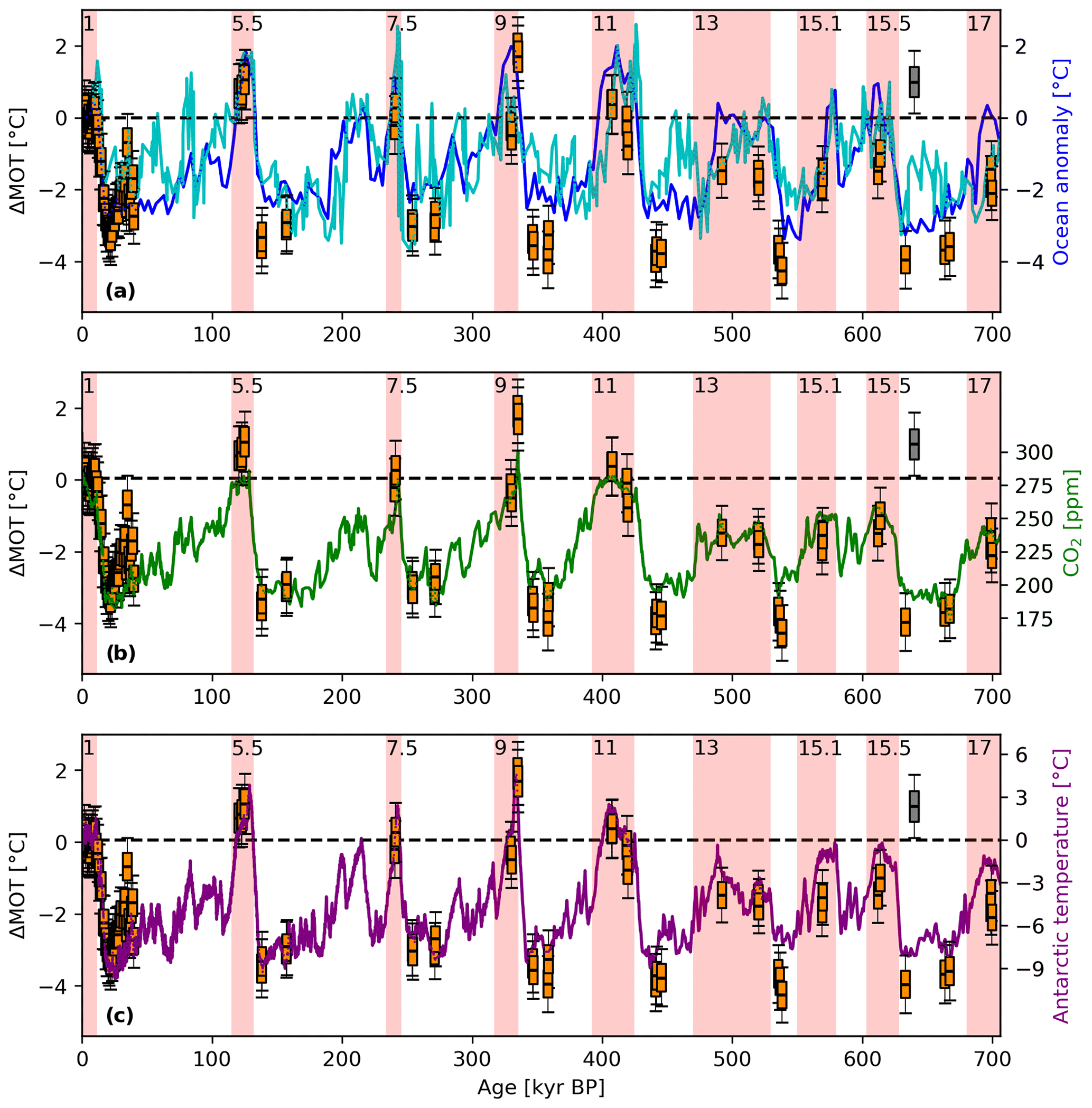
Figure 9MOT record relative to the Holocene from the ratios in comparison with other climate records. The EDC record is based on 85 samples, which are displayed as orange boxes (except one outlier at 638 kyr BP indicated in grey). The uncertainty is shown as described in Sect. 2.3. (a) Deep-ocean reconstructions from a global compilation of 49 paired planktic δ18O records are shown in dark blue (Shakun et al., 2015). Given in cyan is the benthic -derived temperature from Elderfield et al. (2012). (b) The CO2 record is based on measurements from the EDC and Vostok ice core (Nehrbass-Ahles et al., 2020; Bereiter et al., 2015; Lüthi et al., 2008; Petit et al., 1999). (c) Antarctic temperatures are taken from Parrenin et al. (2013). Red shaded bars and MIS numbers on top indicate interglacials according to Masson-Delmotte et al. (2010).
Despite the pointwise character of our data, the -derived MOT record generally supports the main findings from the deep-ocean temperature reconstruction of Elderfield et al. (2012) and Shakun et al. (2015), but in contrast to these studies our record is based on a purely physical proxy and by definition is globally representative for MOT. The main findings are the following.
- i.
Some episodes during the interglacial periods MIS 5.5 and MIS 9.3 are significantly warmer than the Holocene.
- ii.
Glacial MOTs are similar throughout the last 800 kyr, although glacials prior to 450 kyr BP appear slightly colder.
- iii.
The MOTs during interglacial periods prior to 450 kyr BP are significantly colder than after the Mid-Brunhes Event.
Note that each of our samples only represents an MOT snapshot representative of a time interval of a few centuries (Fourteau et al., 2019) given by the width of the gas age distribution for the EDC ice core. Thus individual samples are not representative of the mean interglacial (or glacial) value but may be subject to the millennial-scale variability of MOT. We stress that MOT is strongly influenced by changes in the Atlantic Meridional Overturning Circulation (AMOC) (Baggenstos et al., 2019; Shackleton et al., 2020) and can therefore vary on multi-centennial to millennial timescales, as also seen in coupled climate model experiments (Pedro et al., 2018; Galbraith et al., 2016). A sudden slowdown of the AMOC leads to a long-lasting accumulation of heat in the ocean interior (Pedro et al., 2018; Galbraith et al., 2016; Ritz et al., 2011), while a recovery of the AMOC slowly lowers the MOT. Accordingly, samples very close to the onset of interglacials, which may still be affected by a previously reduced AMOC, may still show elevated MOTs. The heat stored in the global ocean is only removed in the course of 2000–3000 years into the subsequent interglacial after strengthening of the AMOC. This is clearly observed in higher-resolution data for MIS5.5 (Shackleton et al., 2020), which allowed us to temporally resolve this transient feature. Such a deepwater mass reorganization that marks the onset of the subsequent interglacial period is also inferred from changing ocean water tracer distributions (Deaney et al., 2017).
In line with this, our MOT data based on from the onset of MIS 5.5 are on average 1.0 ± 0.4 ∘C warmer than the Holocene and decline to interglacial values only 0.7 ∘C warmer than the Holocene later in MIS5.5. This is in agreement with the findings from Shackleton et al. (2020) that show significantly warmer MOTs reaching a maximum value of 1.1 ± 0.3 ∘C at about 129 kyr BP. Shackleton et al. (2020) attribute the early last interglacial maximum in MOT to the weakening of the AMOC that occurred over termination II during the major iceberg discharge event from Hudson Strait in the North Atlantic commonly known as Heinrich event 11 (Capron et al., 2014). The subsequent release of heat from the ocean after the AMOC resumed led to a MOT decrease of ∼ 1 ∘C with stable MOT only reached after 127 kyr BP.
A similar but even more pronounced ocean warming feature is found in our new data during interglacial MIS 9.3. The samples later in the interglacial (329 and 330 kyr BP) show within uncertainty the same temperatures as the Holocene; however, the very early interglacial samples (334 and 335 kyr BP) show 1.8 ± 0.4 ∘C warmer MOTs than the Holocene. Similarly, global deep-ocean temperatures for early MIS 9.3 compiled from marine sediment records in the study by Shakun et al. (2015) are intermittently nearly 2 ∘C warmer than the Holocene. Our two early MIS 9.3 samples occur also in parallel with a rapid CO2 and CH4 increase at the very end of termination IV. At the onset of interglacial MIS 9.3, Nehrbass-Ahles et al. (2020) measured the highest CO2 values during the last 800 kyr, coeval with the highest CH4 levels (Loulergue et al., 2008) and warm Antarctic temperatures, providing an excellent chronological constraint for the timing of AMOC resumption. An intriguing hypothesis for the high values at the onset of interglacial MIS 9.3 is therefore that the MOT overshoot observed in the final phases of termination IV is also a result of a long preceding period of freshwater-induced AMOC suppression and deepwater mass reorganization (Ganopolski and Brovkin, 2017) that only ended with the AMOC resumption at that time. This suggests, similar to the case in MIS 5.5, that MOT was still elevated by the reduced AMOC in the millennia before and was able to regain interglacial levels several millennia after the rapid CO2 and CH4 increases. This emphasizes the transient character of this feature and the role of an increasing AMOC in Antarctic and ocean temperature as well as in marine and terrestrial biogeochemical cycles.
Our data show glacial mean ocean temperatures very similar throughout the last 800 kyr. On average our measured glacial MOTs are 3.3 ± 0.4 ∘C colder than the Holocene. This is in agreement with the deep-ocean anomaly derived from Elderfield et al. (2012) based on a sediment record from Chatham rise east of New Zealand. There appears to be a slight increasing trend in glacial MOT over the last 700 kyr that is also suggested by the global ocean data compilation of Shakun et al. (2015); however, the trend in our data is of the same order as the uncertainty of our reconstruction. Accordingly, we refrain from interpreting this trend at this point in time; more higher-resolution MOT data are required to show whether this feature persists.
Our data also support the finding of lukewarm interglacials in MOT prior to the Mid-Brunhes Event 450 kyr ago (Shakun et al., 2015; Elderfield et al., 2012), as also seen in Antarctic temperatures (EPICA community members, 2004), but also lower interglacial concentrations of the greenhouse gases CO2 (Bereiter et al., 2015; Lüthi et al., 2008) and CH4 (Loulergue et al., 2008), at least for MIS 13–17. Thus, a potential compensation for the excess effective energy not used for ice sheet melting during lukewarm interglacials, as discussed in the Introduction, can be ruled out based on our ice core and the marine sediment data. Accordingly, the lukewarm interglacials must be connected to a net change in the radiative balance of the globe compared to later warmer interglacials. The MOT anomaly relative to the Holocene during the interglacials MIS 13, 15.1, 15.5, and 17 is −1.6 ± 0.4, −1.7 ± 0.4, −1.3 ± 0.4, and −1.8 ± 0.4 ∘C, respectively. Interglacial bottom-water temperatures also increased by about 1 ∘C after ∼ 450 kyr BP (Elderfield et al., 2012; Shakun et al., 2015); however, Holocene bottom-water temperatures seem to be colder again than during the three preceding interglacials MIS 5.5, MIS 9.3, and MIS 11. Using the global benthic δ18O stack by Lisiecki and Raymo (2005), Bintanja et al. (2005) reconstructed global ice volume changes and the contributions of individual ice sheets back in time. Again, the lukewarm interglacials are significantly different compared to the later interglacials in this model reconstruction and are characterized by up to 20 m lower sea level compared to the Holocene, with the largest contribution to this sea level reduction caused by larger ice sheets in Eurasia. Note, however, that sea levels lower than in the Holocene during lukewarm interglacials can be observed in some but not all sea level reconstructions from marine sediments (Rohling et al., 2014; Spratt and Lisiecki, 2016). In any case, an increase in ice volume during lukewarm interglacials cannot be easily attributed to changes in orbital forcing, as the effective energy at high northern latitudes (Tzedakis et al., 2017) during these intervals did not significantly differ from the insolation conditions during later interglacials. Thus, the lukewarm interglacials require additional changes in the Earth system that prevented Northern Hemisphere ice sheets from retreating and temperatures from increasing to the same extent as in later interglacials.
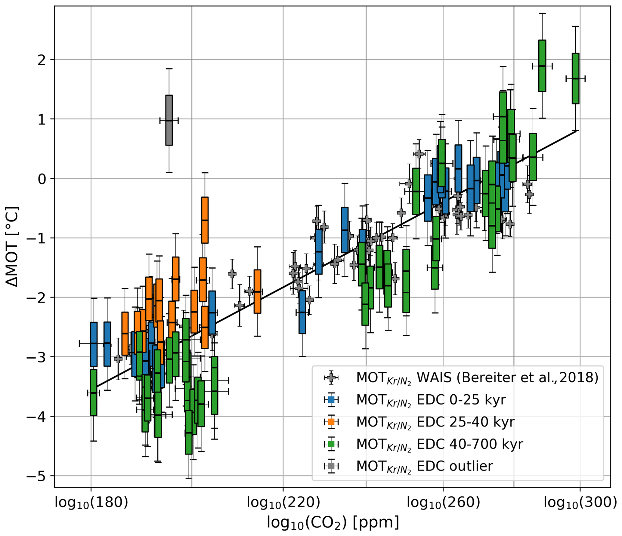
Figure 10Scatter plot showing a linear relationship between logarithmic CO2 (values taken from Bereiter et al., 2015) and the MOT relative to the Holocene. MOT reconstructions are based on and corrected for thermal, gravitational, and HID fractionation. MOTs from the last 25 kyr are shown in blue, samples from 25–40 kyr BP are shown in orange, and samples from 120 to 700 kyr BP are in green. The linear regression (black line) is based on EDC data only and has an r2 of 0.75. Given in grey is the MOT reconstruction over the last 22 kyr from Bereiter et al. (2018b) relative to the Holocene.
Irrespective of the ultimate cause of the incomplete deglaciation during the lukewarm interglacials, our significantly lower MOT values during these lukewarm interglacials provide robust evidence for a significantly altered energy budget of our planet compared to the Holocene. Note that an MOT lowering of about 1 ∘C translates into a decrease in the ocean heat content of 5–6×1024 J, or about 30 % of our typical glacial–interglacial change in heat content. We can estimate whether the deviation in climate boundary conditions (greenhouse gas concentrations and albedo) is sufficient to explain the heat deficit. Lukewarm interglacial CO2 concentrations are typically 245 ppm (instead of 280 ppm in later interglacials) and CH4 concentrations 620 ppb (instead of 700 ppb thereafter). This translates into a radiative forcing of about −0.8 W m−2 (Myhre et al., 1998), and using a recent paleo-based value of the equilibrium climate sensitivity of 3.8 ∘C for a doubling of CO2 (Tierney et al., 2020) (which includes fast feedbacks such as sea ice coverage) it translates into a reduction of the global mean surface temperature (GMST) of about 0.8 ∘C. In addition, we also need to take into account the long-term Earth system feedbacks such as planetary albedo increase due to extended land ice coverage. For the LGM, the fraction of greenhouse gas forcing to total forcing has been estimated as approximately 0.4 (Baggenstos et al., 2019). Using the greenhouse gas forcing for the lukewarm interglacials as given above, the estimated total forcing is thus close to 2 W m−2, which yields an expected GMST decrease of 2.0 ∘C for the lukewarm interglacials. However, comparing global surface temperature to MOT is not straightforward (Bereiter et al., 2018b) because (i) MOT is biased towards sea surface temperatures in deepwater formation regions, for example in the North Atlantic, and is thus subject to polar amplification, and (ii) land temperature change is poorly known and cannot easily be linked to MOT change. However, a recent study has tightly constrained LGM GMST change to 6 ∘C (Tierney et al., 2020), which goes along with an approximately 3 ∘C MOT change for the LGM. Assuming this relationship also holds for earlier interglacials, we scale our average MOT decrease of 1.6 ∘C into a GMST reduction of 3.2 ∘C. This is somewhat larger than the expected GMST lowering of 2.0 ∘C due to radiative forcing and suggests that either the ratio of greenhouse gas forcing to total forcing or the scaling from MOT to GMST was different during the lukewarm interglacials. Note, however, that both of these factors are poorly constrained, and, for example, using 0.3 instead of 0.4 for the forcing ratio along with a slightly smaller MOT and GMST scaling would bring the two estimates into agreement. Thus, our MOT lowering during lukewarm interglacials is within the range expected from the radiative forcing caused by the lower CO2 and CH4 in those intervals and the connected longer-term Earth system feedbacks.
The close relationship of MOT and global radiative forcing with changing greenhouse gas concentrations is not only valid for lukewarm vs. full interglacials but to first order also holds for the entire noble-gas-based MOT record available so far. Bereiter et al. (2018b) showed that MOT is closely correlated with Antarctic temperature and the MOT evolution is essentially synchronous with CO2 during the last transition. Our record from the last 40 kyr supports this correlation. The scatter plot presented in Fig. 10 shows the correlation between MOT and logarithmic CO2, as expected from the radiative forcing of surface temperatures by CO2 concentration (IPCC, 2013). The squared correlation coefficient for all the reconstructed MOTs from EDC and logarithmic CO2 suggests that 75 % of the variance in the MOT record can be explained by changing CO2 and the accompanying Earth system feedbacks. Taking a closer look at Fig. 10 we see again that the peak glacials and the lukewarm interglacials prior to 450 kyr BP show approximately 1 ∘C colder temperatures than expected from the CO2 relationship derived for the last 40 kyr. In view of the considerable systematic uncertainties introduced by the correction of the data, we refrain from speculating on a possible cause of these lower temperatures at this point.
Our study presents MOT snapshots of peak glacial and interglacial periods during the last 700 kyr. The comparison of MOT values derived from different elemental ratios revealed systematically lower MOTs based on and values from the BCTZ and higher MOTs from and in the ice deeper than 2500 m. We attribute this to a Xe depletion during clathrate formation through its low permeation coefficient and/or reduced incorporation of Xe in SII clathrates in the ice. This leads to an enrichment of Xe in bubbles in the BCTZ and a depletion of Xe in reforming PLIs in the deep ice. Together with gas loss through post-coring microcracks, this leads to a depletion of Xe relative to N2 and Kr in the BCTZ and an enrichment in the deep ice. Continuing work on understanding firn gas, especially the HID, is crucial to reduce the uncertainties of the MOT reconstructions based on noble gases.
Despite these limitations we find that glacial MOTs based on , which appear to be free of gas loss and fractionation processes, are on average 3.3 ± 0.4 ∘C colder than the Holocene throughout this noble gas record and that the MOTs during interglacial periods prior to 450 kyr BP are on average 1.6 ± 0.4 ∘C lower compared to the Holocene. Episodes during the onsets of interglacials MIS 5.5 and 9.3 are significantly warmer than the Holocene and can be attributed to the ocean heat uptake during preceding times of lowered AMOC. The most pronounced feature of the record is the significantly increased MOT at the onset of MIS 9.3, which is coeval with the CO2 and CH4 overshoot at that time and reflects maximum ocean heat uptake before the AMOC resumption.
Our data provide only snapshots of MOT in glacial and interglacial conditions; however, these define the natural range in which the global heat budget has changed over the last 700 kyr. Our data show that the range in MOT can be quantitatively explained by changes in global radiative forcing (due to changes in greenhouse gas concentrations), taking into account long-term Earth system feedbacks, and that MOT is biased towards sea surface temperature changes in high latitudes. More high-resolution and high-precision MOT data from noble gases in ice cores (avoiding gas loss issues) and a better understanding of the firn fractionation processes affecting the gas composition in ice cores are needed to make use of the full potential of noble-gas-derived MOT in future studies.
Noble gas data derived in this study will be made available on the NOAA paleoclimate database at https://www.ncdc.noaa.gov/paleo/study/33072 (Haeberli et al., 2021, last access: 31 March 2021). The Python code used for the correction of the data will be made available on request.
The concept of this study was created by HF, JS, and TK, and the research was supported by third-party funding by HF. The analytical method was established by TK, DB, and MH with input by JS and HF. The sample analyses were performed by MH and DB. Data evaluation was performed by MG and MH with inputs from DB and HF. The paper was written by HF and MH, with support by all coauthors, who also contributed heavily to the discussion of the data.
The authors declare that they have no conflict of interest.
We thank Eric Wolff, Gregory Teste, and Catherine Ritz for their help with sample selection and cutting. Catherine Ritz kindly provided borehole temperature profiles at Dome C. Most helpful discussions on noble gases as well as gas and heat transport in the firn with Jeff Severinghaus, Benjamin Birner, Sarah Shackleton, Bernhard Bereiter, and Jakob Schwander are gratefully acknowledged. The research leading to these results has received funding from the European Research Council (ERC) under the European Union's Seventh Framework Programme FP7/2007-2013 through ERC grant 226172 (ERC Advanced Grant Modern Approaches to Temperature Reconstructions in Polar Ice Cores (MATRICs)) and the Swiss National Science Foundation (grant numbers 200021-155906, 200020-172506). This work is a contribution to EPICA, a joint European Science Foundation/European Commission scientific program funded by the European Union and national contributions from Belgium, Denmark, France, Germany, Italy, The Netherlands, Norway, Sweden, Switzerland, and the United Kingdom. The main logistic support was provided by the Institut Polaire Français Paul-Emile Victor (IPEV), PNRA (at Dome C), and AWI (at EDML). This work is EPICA publication no. 317.
This research has been supported by the European Research Council (grant no. 226172) and the Swiss National Science Foundation (SNF) (grant nos. 200021-155906, 200020-172506).
This paper was edited by Amaelle Landais and reviewed by Jeff Severinghaus and one anonymous referee.
Baggenstos, D., Häberli, M., Schmitt, J., Shackleton, S. A., Birner, B., Fischer, H., Severinghaus, J., and Kellerhals, T.: The Earth's radiative imbalance from the Last Glacial Maximum to the present, P. Natl. Acad. Sci. USA, 110, 14881–14886, https://doi.org/10.1073/pnas.1905447116, 2019. a, b, c, d, e
Bazin, L., Landais, A., Lemieux-Dudon, B., Toyé Mahamadou Kele, H., Veres, D., Parrenin, F., Martinerie, P., Ritz, C., Capron, E., Lipenkov, V., Loutre, M.-F., Raynaud, D., Vinther, B., Svensson, A., Rasmussen, S. O., Severi, M., Blunier, T., Leuenberger, M., Fischer, H., Masson-Delmotte, V., Chappellaz, J., and Wolff, E.: An optimized multi-proxy, multi-site Antarctic ice and gas orbital chronology (AICC2012): 120–800 ka, Clim. Past, 9, 1715–1731, https://doi.org/10.5194/cp-9-1715-2013, 2013. a
Bender, M., Sowers, T., and Lipenkov, V.: On the concentrations of O2, N2, and Ar in trapped gases from ice cores, J. Geophys. Res., 100, 18651, https://doi.org/10.1029/94JD02212, 1995. a
Bender, M. L.: Orbital tuning chronology for the Vostok climate record supported by trapped gas composition, Earth Planet. Sc. Lett., 204, 275–289, https://doi.org/10.1016/S0012-821X(02)00980-9, 2002. a
Bender, M. L., Barnett, B., Dreyfus, G., Jouzel, J., and Porcelli, D.: The contemporary degassing rate of 40Ar from the solid Earth, P. Natl. Acad. Sci. USA, 105, 8232–8237, https://doi.org/10.1073/pnas.0711679105, 2008. a, b, c
Bereiter, B., Schwander, J., Lüthi, D., and Stocker, T. F.: Change in CO2 concentration and ratio in ice cores due to molecular diffusion, Geophys. Res. Lett., 36, L05703, https://doi.org/10.1029/2008GL036737, 2009. a
Bereiter, B., Eggleston, S., Schmitt, J., Nehrbass-Ahles, C., Stocker, T. F., Fischer, H., Kipfstuhl, S., and Chappellaz, J.: Revision of the EPICA Dome CO2 record from 800 to 600 kyr before present, Geophys. Res. Lett., 42, 542–549, https://doi.org/10.1002/2014GL061957, 2015. a, b, c, d
Bereiter, B., Kawamura, K., and Severinghaus, J. P.: New methods for measuring atmospheric heavy noble gas isotope and elemental ratios in ice core samples, Rapid Commun. Mass Sp., 32, 801–814, https://doi.org/10.1002/rcm.8099, 2018a. a, b, c
Bereiter, B., Shackleton, S., Baggenstos, D., Kawamura, K., and Severinghaus, J.: Mean global ocean temperatures during the last glacial transition, Nature, 553, 39, https://doi.org/10.1038/nature25152, 2018b. a, b, c, d, e, f, g, h, i
Bintanja, R., Van De Wal, R. S., and Oerlemans, J.: Modelled atmospheric temperatures and global sea levels over the past million years, Nature, 437, 125–128, https://doi.org/10.1038/nature03975, 2005. a, b
Birner, B., Buizert, C., Wagner, T. J. W., and Severinghaus, J. P.: The influence of layering and barometric pumping on firn air transport in a 2-D model, The Cryosphere, 12, 2021–2037, https://doi.org/10.5194/tc-12-2021-2018, 2018. a, b, c, d, e, f, g, h, i, j, k, l
Bréant, C., Landais, A., Orsi, A., Martinerie, P., Extier, T., Prié, F., Stenni, B., Jouzel, J., Masson-Delmotte, V., and Leuenberger, M.: Unveiling the Anatomy of Termination 3 Using Water and Air Isotopes in the Dome C Ice Core, East Antarctica, Quat. Sci. Rev., 211, 156–165, https://doi.org/10.1016/j.quascirev.2019.03.025, 2019. a, b
Buizert, C. and Severinghaus, J. P.: Dispersion in deep polar firn driven by synoptic-scale surface pressure variability, The Cryosphere, 10, 2099–2111, https://doi.org/10.5194/tc-10-2099-2016, 2016. a, b, c, d, e
Buizert, C., Fudge, T., Roberts, W., Steig, E., Sherriff-Tadano, S., Ritz, C., Lefebvre, E., Kawamura, K., Oyabu, I., Motoyama, H., Kahle, E., Jones, T., Abe-Ouchi, A., Obase, T., Martin, C., Corr, H., Severinghaus, J., Beaudette, R., Epifanio, J., Brook, E., Martin, K., Chappellaz, J., Aoki, S., Nakazawa, T., Sowers, T., Ahn, J., Sigl, M., Severi, M., Dunbar, N., Svensson, A., Schwander, J., and Johnsen, S.: A revision of last glacial maximum temperatures in East Antarctica, submitted to Science, 2020. a, b
Capron, E., Govin, A., Stone, E. J., Masson-Delmotte, V., Mulitza, S., Otto-Bliesner, B., Rasmussen, T. L., Sime, L. C., Waelbroeck, C., and Wolff, E. W.: Temporal and spatial structure of multi-millennial temperature changes at high latitudes during the Last Interglacial, Quat. Sci. Rev., 103, 116–133, https://doi.org/10.1016/j.quascirev.2014.08.018, 2014. a
Craig, H. and Wiens, R.: Gravitational enrichment of 84Kr/36Ar ratios in polar ice caps: A measure of firn thickness and accumulation temperature, Science, 271, 1708–1710, 1996. a
Craig, H., Horibe, Y., and Sowers, T.: Gravitational Separation of Gases and Isotopes in Polar Ice Caps, Science, 242, 1675–1678, https://doi.org/10.1126/science.242.4886.1675, 1988. a
Cuffey, K. M. and Paterson, W. S. B.: The temperatures in ice masses, Butterworth-Heinemann, Burlington, MA, 704 pp., 2010. a
Deaney, E. L., Barker, S., and van de Flierdt, T.: Timing and nature of AMOC recovery across Termination 2 and magnitude of deglacial CO2 change, Nat. Commun., 8, 14595, https://doi.org/10.1038/ncomms14595, 2017. a
Dreyfus, G. B., Jouzel, J., Bender, M. L., Landais, A., Masson-Delmotte, V., and Leuenberger, M.: Firn Processes and δ15N: Potential for a Gas-Phase Climate Proxy, Quat. Sci. Rev., 29, 28–42, https://doi.org/10.1016/j.quascirev.2009.10.012, 2010. a, b
Durand, G., Svensson, A., Persson, A., Gagliardini, O., Gillet-Chaulet, F., Sjolte, J., Montagnat, M., and Dahl-Jensen, D.: Evolution of the texture along the EPICA Dome C ice core, Low Temp. Sci., 68, 91–105, https://eprints.lib.hokudai.ac.jp/dspace/handle/2115/45436 (last access: 28 March 2021), 2009. a, b
Dutton, A., Carlson, A. E., Long, A. J., Milne, G. A., Clark, P. U., DeConto, R., Horton, B. P., Rahmstorf, S., and Raymo, M. E.: Sea-level rise due to polar ice-sheet mass loss during past warm periods, Science, 349, aaa4019, https://doi.org/10.1126/science.aaa4019, 2015. a
Elderfield, H., Ferretti, P., Greaves, M., Crowhurst, S., McCave, I. N., Hodell, D., and Piotrowski, A. M.: Evolution of Ocean Temperature and Ice Volume Through the Mid-Pleistocene Climate Transition, Science, 337, 704–709, https://doi.org/10.1126/science.1221294, 2012. a, b, c, d, e, f, g
EPICA community members: Eight glacial cycles from an Antarctic ice core., Nature, 429, 623–628, https://doi.org/10.1038/nature02599, 2004. a, b, c, d
Extier, T., Landais, A., Bréant, C., Prié, F., Bazin, L., Dreyfus, G., Roche, D. M., and Leuenberger, M.: On the use of δ18Oatmfor ice core dating, Quat. Sci. Rev., 185, 244–257, https://doi.org/10.1016/j.quascirev.2018.02.008, 2018. a, b, c, d, e
Fourteau, K., Martinerie, P., Faïn, X., Schaller, C. F., Tuckwell, R. J., Löwe, H., Arnaud, L., Magand, O., Thomas, E. R., Freitag, J., Mulvaney, R., Schneebeli, M., and Lipenkov, V. Ya.: Multi-tracer study of gas trapping in an East Antarctic ice core, The Cryosphere, 13, 3383–3403, https://doi.org/10.5194/tc-13-3383-2019, 2019. a
Galbraith, E. D., Merlis, T. M., and Palter, J. B.: Destabilization of glacial climate by the radiative impact of Atlantic Meridional Overturning Circulation disruptions, Geophys. Res. Lett., 43, 8214–8221, https://doi.org/10.1002/2016GL069846, 2016. a, b
Ganopolski, A. and Brovkin, V.: Simulation of climate, ice sheets and CO2 evolution during the last four glacial cycles with an Earth system model of intermediate complexity, Clim. Past, 13, 1695–1716, https://doi.org/10.5194/cp-13-1695-2017, 2017. a
Gleckler, P. J., Durack, P. J., Stouffer, R. J., Johnson, G. C., and Forest, C. E.: Industrial-era global ocean heat uptake doubles in recent decades, Nat. Clim. Change, 6, 394–398, https://doi.org/10.1038/nclimate2915, 2016. a
Hamme, R. C. and Severinghaus, J. P.: Trace gas disequilibria during deep-water formation, Deep Sea-Res. Pt. I, 54, 939–950, https://doi.org/10.1016/j.dsr.2007.03.008, 2007. a
Hamme, R. C., Nicholson, D. P., Jenkins, W. J., and Emerson, S. R.: Using Noble Gases to Assess the Ocean's Carbon Pumps, Annu. Rev. Mar. Sci., 11, 75–103, https://doi.org/10.1146/annurev-marine-121916-063604, 2019. a
Headly, M. A.: Krypton and xenon in air trapped in polar ice cores: Paleo-atmospheric measurements for estimating past mean ocean temperature and summer snowmelt frequency, PhD thesis, University of California, San Diego, 229 pp., 2008. a, b
Headly, M. A. and Severinghaus, J. P.: A method to measure Kr/N2 ratios in air bubbles trapped in ice cores and its application in reconstructing past mean ocean temperature, J. Geophys. Res.-Atmos., 112, D19105, https://doi.org/10.1029/2006jd008317, 2007. a
Hoffman, J. S., Clark, P. U., Parnell, A. C., and He, F.: Regional and global sea-surface temperatures during the last interglaciation, Science, 355, 276–279, https://doi.org/10.1126/science.aai8464, 2017. a
Ikeda, T., Salamatin, A. N., Lipenkov, V. Y., Mae, S., and Hondoh, T.: Spatial distribution of air molecules within individual clathrate hydrates in polar ice sheets, in: Annals of Glaciology, Vol. 31, 2000, edited by: Steffen, K., Vol. 31 of Annals of Glaciology, 252–256, Int Glaciol Soc; ETH; Univ Zurich; Schweizer Akad Nat Wissensch; Schweizer Stift Alphine Forsch, Int glaciological soc, Lensfield rd, Cambridge, England, CB2 1er, https://doi.org/10.3189/172756400781820390, 2000. a
Ikeda-Fukazawa, T., Fukumizu, K., Kawamura, K., Aoki, S., Nakazawa, T., and Hondoh, T.: Effects of molecular diffusion on trapped gas composition in polar ice cores, Earth Planet. Sc. Lett., 229, 183–192, https://doi.org/10.1016/j.epsl.2004.11.011, 2005. a
IPCC: IPCC Climate Change 2013: The Physical Science Basis, edited by: Stocker, T. F., Dahe, Q., Plattner, G.-K., Tignor, M. M. B., Allen, S. K., Boschung, J., Nauels, A., Yu, X., Bex, V., and Midgley, P. M., Cambridge Univ. Press, Cambridge, 1535 pp., 2013. a
Jenkins, W., Lott, D., and Cahill, K.: A Determination of Atmospheric Helium, Neon, Argon, Krypton, and Xenon Solubility Concentrations in Water and Seawater, Mar. Chem., 211, 94–107, https://doi.org/10.1016/j.marchem.2019.03.007, 2019. a
Kawamura, K., Parrenin, F., Lisiecki, L., Uemura, R., Vimeux, F., Severinghaus, J. P., Hutterli, M. A., Nakazawa, T., Aoki, S., Jouzel, J., Raymo, M. E., Matsumoto, K., Nakata, H., Motoyama, H., Fujita, S., Goto-Azuma, K., Fujii, Y., and Watanabe, O.: Northern Hemisphere forcing of climatic cycles in Antarctica over the past 360,000 years, Nature, 448, 912–916, https://doi.org/10.1038/nature06015, 2007. a
Kawamura, K., Severinghaus, J. P., Albert, M. R., Courville, Z. R., Fahnestock, M. A., Scambos, T., Shields, E., and Shuman, C. A.: Kinetic fractionation of gases by deep air convection in polar firn, Atmos. Chem. Phys., 13, 11141–11155, https://doi.org/10.5194/acp-13-11141-2013, 2013. a, b, c, d, e
Kobashi, T., Severinghaus, J. P., and Barnola, J.-M.: 4 ± 1.5 ∘C abrupt warming 11,270 yr ago identified from trapped air in Greenland ice, Earth Planet. Sc. Lett., 268, 397–407, https://doi.org/10.1016/j.epsl.2008.01.032, 2008a. a
Kobashi, T., Severinghaus, J. P., and Kawamura, K.: Argon and nitrogen isotopes of trapped air in the GISP2 ice core during the Holocene epoch (0-11,500 B.P.): Methodology and implications for gas loss processes, Geochim. Cosmochim. Ac., 72, 4675–4686, https://doi.org/10.1016/j.gca.2008.07.006, 2008b. a
Lambeck, K., Rouby, H., Purcell, A., Sun, Y., and Sambridge, M.: Sea level and global ice volumes from the Last Glacial Maximum to the Holocene, P. Natl. Acad. Sci. USA, 111, 15296–15303, https://doi.org/10.1073/pnas.1411762111, 2014. a
Landais, A., Dreyfus, G., Capron, E., Pol, K., Loutre, M. F., Raynaud, D., Lipenkov, V. Y., Arnaud, L., Masson-Delmotte, V., Paillard, D., Jouzel, J., and Leuenberger, M.: Towards orbital dating of the EPICA Dome C ice core using , Clim. Past, 8, 191–203, https://doi.org/10.5194/cp-8-191-2012, 2012. a
Landais, A., Dreyfus, G., Capron, E., Jouzel, J., Masson-Delmotte, V., Roche, D. M., Prié, F., Caillon, N., Chappellaz, J., Leuenberger, M., Lourantou, A., Parrenin, F., Raynaud, D., and Teste, G.: Two-Phase Change in CO2, Antarctic Temperature and Global Climate during Termination II, Nat. Geosci., 6, 1062–1065, https://doi.org/10.1038/ngeo1985, 2013. a, b
Lipenkov, V.: Air bubbles and air-hydrate crystals in the Vostok ice core, Physics of Ice Core Records, 327–358, 2000. a
Lisiecki, L. E. and Raymo, M. E.: A Pliocene-Pleistocene stack of 57 globally distributed benthic δ18O records, Paleoceanography, 20, PA1003, https://doi.org/10.1029/2005PA001164, 2005. a, b
Loose, B., Jenkins, W. J., Moriarty, R., Brown, P., Jullion, L., Naveira Garabato, A. C., Torres Valdes, S., Hoppema, M., Ballentine, C., and Meredith, M. P.: Estimating the recharge properties of the deep ocean using noble gases and helium isotopes, J. Geophys. Res.-Oceans, 121, 5959–5979, https://doi.org/10.1002/2016JC011809, 2016. a
Loulergue, L., Schilt, A., Spahni, R., Masson-Delmotte, V., Blunier, T., Lemieux, B., Barnola, J.-M., Raynaud, D., Stocker, T. F., and Chappellaz, J.: Orbital and millennial-scale features of atmospheric, Nature, 453, 383–386, https://doi.org/10.1038/nature06950, 2008. a, b
Lüthi, D., Le Floch, M., Bereiter, B., Blunier, T., Barnola, J.-M., Siegenthaler, U., Raynaud, D., Jouzel, J., Fischer, H., Kawamura, K., and Stocker, T. F.: High-resolution carbon dioxide concentration record 650,000–800,000 years before present, Nature, 453, 379, https://doi.org/10.1038/nature06949, 2008. a, b
Masson-Delmotte, V., Stenni, B., Pol, K., Braconnot, P., Cattani, O., Falourd, S., Kageyama, M., Jouzel, J., Landais, A., Minster, B., Barnola, J. M., Chappellaz, J., Krinner, G., Johnsen, S., Röthlisberger, R., Hansen, J., Mikolajewicz, U., and Otto-Bliesner, B.: EPICA Dome C record of glacial and interglacial intensities, Quat. Sci. Rev., 29, 113–128, https://doi.org/10.1016/j.quascirev.2009.09.030, 2010. a, b, c, d, e, f, g, h
Melles, M., Brigham-Grette, J., Minyuk, P. S., Nowaczyk, N. R., Wennrich, V., DeConto, R. M., Anderson, P. M., Andreev, A. A., Coletti, A., Cook, T. L., Haltia-Hovi, E., Kukkonen, M., Lozhkin, A. V., Rosén, P., Tarasov, P., Vogel, H., and Wagner, B.: 2.8 Million Years of Arctic Climate Change from Lake El'gygytgyn, NE Russia, Science, 337, 315–320, https://doi.org/10.1126/science.1222135, 2012. a
Michel, A.: Transient modeling of borehole temperature and basal melting in an ice sheet, Master thesis, University of Bern, 125 pp., 2016. a, b, c, d, e, f, g
Milankovic, M.: Kanon der Erdbestrahlung und seine Anwendung auf das Eiszeitenproblem. Belgrade, Royal Serbian Acad. Sciences, Spec. Publ. 132, Sect. Math, Nat. Sci, 33, 633 pp., 1941. a
Myhre, G., Highwood, E. J., Shine, K. P., and Stordal, F.: New estimates of radiative forcing due to well mixed greenhouse gases, Geophys. Res. Lett., 25, 2715–2718, https://doi.org/10.1029/98GL01908, 1998. a
Nedelcu, A. F., Faria, S. H., and Kuhs, W. F.: Raman spectra of plate-like inclusions in the EPICA-DML (Antarctica) ice core, J. Glaciol., 55, 183–184, https://doi.org/10.3189/002214309788609010, 2009. a, b, c, d
Neff, P. D.: A review of the brittle ice zone in polar ice cores, Ann. Glaciol., 55, 72–82, https://doi.org/10.3189/2014AoG68A023, 2014. a
Nehrbass-Ahles, C., Shin, J., Schmitt, J., Bereiter, B., Joos, F., Schilt, A., Schmidely, L., Silva, L., Teste, G., Grilli, R., Chappellaz, J., Hodell, D., Fischer, H., and Stocker, T. F.: Abrupt CO2 release to the atmosphere under glacial and early interglacial climate conditions, Science, 369, 1000–1005, https://doi.org/10.1126/science.aay8178, 2020. a, b
PAGES Past Interglacials Working Group, o. p.: Interglacials of the last 800,000 years, Rev. Geophys., 54, 162–219, https://doi.org/10.1002/2015RG000482, 2016. a
Parrenin, F., Barnola, J.-M., Beer, J., Blunier, T., Castellano, E., Chappellaz, J., Dreyfus, G., Fischer, H., Fujita, S., Jouzel, J., Kawamura, K., Lemieux-Dudon, B., Loulergue, L., Masson-Delmotte, V., Narcisi, B., Petit, J.-R., Raisbeck, G., Raynaud, D., Ruth, U., Schwander, J., Severi, M., Spahni, R., Steffensen, J. P., Svensson, A., Udisti, R., Waelbroeck, C., and Wolff, E.: The EDC3 chronology for the EPICA Dome C ice core, Clim. Past, 3, 485–497, https://doi.org/10.5194/cp-3-485-2007, 2007. a
Parrenin, F., Masson-Delmotte, V., Koehler, P., Raynaud, D., Paillard, D., Schwander, J., Barbante, C., Landais, A., Wegner, A., and Jouzel, J.: Synchronous change of atmospheric CO2 and antarctic temperature during the last deglacial warming, Science, 339, 1060–1063, https://doi.org/10.1126/science.1226368, 2013. a
Pedro, J. B., Jochum, M., Buizert, C., He, F., Barker, S., and Rasmussen, S. O.: Beyond the bipolar seesaw: Toward a process understanding of interhemispheric coupling, Quat. Sci. Rev., 192, 27–46, https://doi.org/10.1016/j.quascirev.2018.05.005, 2018. a, b
Petit, J. R., Jouzel, J., Raynaud, D., Barkov, N. I., Barnola, J.-M., Basile, I., Bender, M., Chappellaz, J., Davis, M., Delaygue, G., Delmotte, M., Kotlyakov, V. M., Legrand, M., Lipenkov, V. Y., Lorius, C., Pepin, L., Ritz, C., Saltzman, E., and Stievenard, M.: Climate and atmospheric history of the past 420,000 years from the Vostok ice core, Antarctica, Nature, 399, 429–436, 1999. a
Ritz, C., Lliboutry, L., and Rado, C.: Analysis of a 870 m Deep Temperature Profile at Dome C, Ann. Glaciol., 3, 284–289, https://doi.org/10.3189/S0260305500002937, 1982. a
Ritz, S. P., Stocker, T. F., and Severinghaus, J. P.: Noble gases as proxies of mean ocean temperature: Sensitivity studies using a climate model of reduced complexity, Quat. Sci. Rev., 30, 3728–3741, https://doi.org/10.1016/j.quascirev.2011.09.021, 2011. a, b
Rohling, E. J., Foster, G. L., Grant, K. M., Marino, G., Roberts, A. P., Tamisiea, M. E., and Williams, F.: Sea-level and deep-sea-temperature variability over the past 5.3 million years, Nature, 508, 477–482, https://doi.org/10.1038/nature13230, 2014. a
Schwander, J.: Gas Diffusion in Firn, in: Chemical Exchange Between the Atmosphere and Polar Snow, Springer Berlin Heidelberg, Berlin, Heidelberg, 527–540, https://doi.org/10.1007/978-3-642-61171-1{_}22, 1996. a
Schwander, J., Stauffer, B., and Sigg, A.: Air mixing in firn and the age of the air at pore close-off, Ann. Glaciol., 10, 141–145, https://doi.org/10.1017/S0260305500004328, 1988. a
Seltzer, A. M., Pavia, F. J., Ng, J., and Severinghaus, J. P.: Heavy Noble Gas Isotopes as New Constraints on the Ventilation of the Deep Ocean, Geophys. Res. Lett., 46, 8926–8932, https://doi.org/10.1029/2019GL084089, 2019. a
Severinghaus, J. P. and Battle, M. O.: Fractionation of gases in polar lee during bubble close-off: New constraints from firn air Ne, Kr and Xe observations, Earth Planet. Sc. Lett., 244, 474–500, https://doi.org/10.1016/j.epsl.2006.01.032, 2006. a
Severinghaus, J. P., Grachev, A., Luz, B., and Caillon, N.: A method for precise measurement of argon 40/36 and krypton/argon ratios in trapped air in polar ice with applications to past firn thickness and abrupt climate change in Greenland and at Siple Dome, Antarctica, Geochim. Cosmochim. Ac., 67, 325–343, https://doi.org/10.1016/s0016-7037(02)00965-1, 2003. a, b
Shackleton, S., Baggenstos, D., Menking, J. A., Dyonisius, M. N., Bereiter, B., Bauska, T. K., Rhodes, R. H., Brook, E. J., Petrenko, V. V., McConnell, J. R., Kellerhals, T., Häberli, M., Schmitt, J., Fischer, H., and Severinghaus, J. P.: Global ocean heat content in the Last Interglacial, Nat. Geosci., 13, 77–81, https://doi.org/10.1038/s41561-019-0498-0, 2020. a, b, c, d, e, f, g
Shakun, J. D., Clark, P. U., He, F., Marcott, S. A., Mix, A. C., Liu, Z., Otto-Bliesner, B., Schmittner, A., and Bard, E.: Global warming preceded by increasing carbon dioxide concentrations during the last deglaciation, Nature, 484, 49–54, https://doi.org/10.1038/nature10915, 2012. a
Shakun, J. D., Lea, D. W., Lisiecki, L. E., and Raymo, M. E.: An 800-kyr record of global surface ocean δ18O and implications for ice volume-temperature coupling, Earth Planet. Sc. Lett., 426, 58–68, https://doi.org/10.1016/j.epsl.2015.05.042, 2015. a, b, c, d, e, f, g, h, i
Sloan, E. D. and Koh, C. A.: Clathrate Hydrates of Natural Gases, Third Edition, CRC Press, 3 Edn., https://doi.org/10.1201/9781420008494, 2007. a
Spratt, R. M. and Lisiecki, L. E.: A Late Pleistocene sea level stack, Clim. Past, 12, 1079–1092, https://doi.org/10.5194/cp-12-1079-2016, 2016. a, b
Stolper, D. A., Bender, M. L., Dreyfus, G. B., Yan, Y., and Higgins, J. A.: A Pleistocene ice core record of atmospheric O2 concentrations, Science, 353, 1427–1430, https://doi.org/10.1126/science.aaf5445, 2016. a
Tierney, J. E., Zhu, J., King, J., Malevich, S. B., Hakim, G. J., and Poulsen, C. J.: Glacial cooling and climate sensitivity revisited, Nature, 584, 569–573, https://doi.org/10.1038/s41586-020-2617-x, 2020. a, b
Tzedakis, P. C., Hooghiemstra, H., and Pälike, H.: The last 1.35 million years at Tenaghi Philippon: revised chronostratigraphy and long-term vegetation trends, Quat. Sci. Rev., 25, 3416–3430, https://doi.org/10.1016/j.quascirev.2006.09.002, 2006. a
Tzedakis, P. C., Crucifix, M., Mitsui, T., and Wolff, E. W.: A simple rule to determine which insolation cycles lead to interglacials, Nature, 542, 427–432, https://doi.org/10.1038/nature21364, 2017. a, b, c, d
Uchida, T., Miyamoto, A., Shin'yama, A., and Hondoh, T.: Crystal growth of air hydrates over 720 ka in Dome Fuji (Antarctica) ice cores: microscopic observations of morphological changes below 2000 m depth, J. Glaciol., 57, 1017–1026, https://doi.org/10.3189/002214311798843296, 2011. a, b, c, d
von Schuckmann, K., Cheng, L., Palmer, M. D., Hansen, J., Tassone, C., Aich, V., Adusumilli, S., Beltrami, H., Boyer, T., Cuesta-Valero, F. J., Desbruyères, D., Domingues, C., García-García, A., Gentine, P., Gilson, J., Gorfer, M., Haimberger, L., Ishii, M., Johnson, G. C., Killick, R., King, B. A., Kirchengast, G., Kolodziejczyk, N., Lyman, J., Marzeion, B., Mayer, M., Monier, M., Monselesan, D. P., Purkey, S., Roemmich, D., Schweiger, A., Seneviratne, S. I., Shepherd, A., Slater, D. A., Steiner, A. K., Straneo, F., Timmermans, M.-L., and Wijffels, S. E.: Heat stored in the Earth system: where does the energy go?, Earth Syst. Sci. Data, 12, 2013–2041, https://doi.org/10.5194/essd-12-2013-2020, 2020. a
Weikusat, C., Freitag, J., and Kipfstuhl, S.: Raman spectroscopy of gaseous inclusions in EDML ice core: first results – microbubbles, J. Glaciol., 58, 761–766, https://doi.org/10.3189/2012JoG11J222, 2012. a, b
Weller, G. and Schwerdtfeger, P.: Thermal properties and heat transfer processes of the snow of the central Antarctic Plateau, in: International Association of Scientific Hydrology, Publication No. 86, 284–298, 1970. a
- Abstract
- Introduction
- Measurement and corrections
- Post-coring gas loss effects on MOT reconstructions
- MOT snapshots of peak glacial and interglacial periods during the last 700 kyr
- Conclusions
- Code and data availability
- Author contributions
- Competing interests
- Acknowledgements
- Financial support
- Review statement
- References