the Creative Commons Attribution 4.0 License.
the Creative Commons Attribution 4.0 License.
 | 06 Apr 2021
Evaluating the biological pump efficiency of the Last Glacial Maximum ocean using δ13C
Jörg Schwinger
Ulysses S. Ninnemann
Aurich Jeltsch-Thömmes
Ingo Bethke
Christoph Heinze
Although both physical and biological marine changes are required to explain the 100 ppm lower atmospheric pCO2 of the Last Glacial Maximum (LGM, ∼21 ka) as compared to preindustrial (PI) times, their exact contributions are debated. Proxies of past marine carbon cycling (such as δ13C) document these changes and thus provide constraints for quantifying the drivers of long-term carbon cycle variability. This modeling study discusses the physical and biological changes in the ocean needed to simulate an LGM ocean in satisfactory agreement with proxy data, here focusing especially on δ13C. We prepared a PI and LGM equilibrium simulation using the ocean model NorESM-OC with full biogeochemistry (including the carbon isotopes δ13C and radiocarbon) and dynamic sea ice. The modeled LGM–PI differences are evaluated against a wide range of physical and biogeochemical proxy data and show agreement for key aspects of the physical ocean state within the data uncertainties. However, the lack of a simulated increase of regenerated nutrients for the LGM indicates that additional biogeochemical changes are required to simulate an LGM ocean in agreement with proxy data. In order to examine these changes, we explore the potential effects of different global mean biological pump efficiencies on the simulated marine biogeochemical tracer distributions. Through estimating which biological pump efficiency reduces LGM model–proxy biases the most, we estimate that the global mean biological pump efficiency increased from 38 % (PI) to up to 75 % (LGM). The drivers of such an increase in the biological pump efficiency may be both biological and related to circulation changes that are incompletely captured by our model – such as stronger isolation of Southern Source Water. Finally, even after considering a 75 % biological pump efficiency in the LGM ocean, a remaining model–proxy error in δ13C exists that is 0.07 ‰ larger than the 0.19 ‰ data uncertainty. This error indicates that additional changes in ocean dynamics are needed to simulate an LGM ocean in agreement with proxy data.
- Article
(2534 KB) - Full-text XML
-
Supplement
(2767 KB) - BibTeX
- EndNote


Model and proxy reconstructions of the Last Glacial Maximum (LGM) suggest major redistributions of marine biogeochemical tracers and water masses as compared to preindustrial (PI) times, as well as lower carbon storage in both the land biosphere and atmosphere. The culmination of these changes into a ∼100 ppm lower LGM atmospheric pCO2 concentration (pCO2atm; EPICA Project Members, 2004) has driven extensive research to identify, understand, and quantify the processes contributing to these major pCO2atm variations (e.g., Broecker, 1982; Broecker and Peng, 1986; Heinze and Hasselmann, 1993; Heinze et al., 2016; Sigman et al., 2010; Adkins, 2013; Jeltsch-Thömmes et al., 2019; Rae et al., 2018). The oceans are of particular interest as they form the largest carbon reservoir available for atmospheric exchange on millennial timescales, and in addition they need to have stored the extra carbon coming from the land biosphere and atmosphere during the LGM. Both physical (circulation, solubility) and biological processes (biological pump efficiency) likely played a role in the differences between the LGM and PI oceans, although their relative importance is under debate. Between ∼25 % and ∼60 % is attributed to biological processes and the remainder to physical changes (Bouttes et al., 2011; Buchanan et al., 2016; Khatiwala et al., 2019; Yamamoto et al., 2019; Kobayashi et al., 2015; Stein et al., 2020; Marzocchi and Jansen, 2019).
LGM model–data comparisons provide a powerful tool to test hypotheses on glacial–interglacial changes of physical–biogeochemical ocean state, to attribute observed changes to processes, and to validate paleoclimatic model simulations. δ13C of DIC (total dissolved inorganic carbon) is a particularly well-suited tracer because it reflects variations in circulation, biological production, and remineralization in parallel and because of the wealth of δ13C measurements available from the sediment core archives. This was demonstrated in previous studies on LGM model–data comparisons involving δ13C (e.g., Tagliabue et al., 2009; Hesse et al., 2011; Gebbie, 2014; Schmittner and Somes, 2016; Menviel et al., 2017; Muglia et al., 2018; Menviel et al., 2020).
Here, we explore the marine physical and biological changes needed to simulate an LGM ocean in optimal agreement with proxy data. We use the concept of the biological pump efficiency (defined as the ability of marine organisms to consume surface ocean phosphate, or more specifically the ratio of global mean regenerated to total phosphate, Sect. 2.4) to examine its effect on LGM marine biogeochemical tracer distributions in concert with physical changes. The global mean efficiency of the biological pump is strongly and nearly linearly correlated with atmospheric CO2 concentrations (Ito and Follows, 2005) and is considered a key concept to understand the atmospheric CO2 drawdown potential of the ocean (Ödalen et al., 2018) through its influence on the vertical gradient of marine dissolved inorganic carbon (DIC). In our evaluation and discussion, we pay particular attention to the role of Southern Source Water (SSW, waters originating in the Southern Ocean), which are thought to be a key component in altering ocean interior tracer distributions and glacial pCO2atm drawdown (e.g., Lynch-Stieglitz et al., 2016; Schmitt et al., 2012; Moy et al., 2019; Sigman et al., 2010; Ferrari et al., 2014; Morée et al., 2018; Khatiwala et al., 2019; Rae et al., 2018; Kobayashi et al., 2015; Marzocchi and Jansen, 2019; Stein et al., 2020).
Our work represents the first LGM simulation using a forced isopycnic ocean model (NorESM-OC; Schwinger et al., 2016; Tjiputra et al., 2020), where all atmospheric forcing fields have been adjusted to represent the LGM (Sect. 2). Besides a general ocean circulation model (MICOM), NorESM-OC simulates full biogeochemistry including the 13C and 14C carbon isotopes (model HAMOCC), as well as dynamic sea ice (model CICE) and a prognostic box atmosphere. The simulation of the carbon isotopes is particularly useful here as they (i) can be directly compared to data from sediment cores (e.g., Gebbie et al., 2015; Skinner et al., 2017), (ii) are influenced by both biological and physical processes (e.g., Broecker and McGee, 2013), (iii) give an indication which oceanic regions could be most relevant (Schmitt et al., 2012; Morée et al., 2018; Skinner et al., 2017), and, given the above, (iv) are useful in model evaluation (Schmittner et al., 2013; Braconnot et al., 2012). We focus on the standardized carbon isotope ratio (δ13C; Zeebe and Wolf-Gladrow, 2001), for which a relatively large number of LGM data are available (e.g., Peterson et al., 2014; Oliver et al., 2010). In addition, the carbon isotope ratio (expressed as Δ14C) provides the model with an age tracer (radiocarbon age), which can be used to understand water mass ventilation and circulation rates and for comparison with reconstructed Δ14C (Skinner et al., 2017; Gebbie and Huybers, 2012). We furthermore evaluate the LGM simulation against proxy and/or model reconstructions of water mass distributions, sea surface temperature, salinity, sea ice extent, export production, vertical nutrient redistribution, pCO2atm, the change in marine dissolved inorganic carbon, and O2 (Sect. 3.2). We apply the concept of true oxygen utilization (TOU; Ito et al., 2004) instead of apparent oxygen utilization (AOU) and make use of the explicit simulation of preformed biogeochemical tracers in our model (Tjiputra et al., 2020). This approach makes it possible to separate physical and biogeochemical drivers of the tracer distributions more thoroughly and accounts for the role of the air–sea carbon disequilibrium pump (Khatiwala et al., 2019). We acknowledge that without a land source of C in our simulated LGM ocean (of ∼850 Gt C, Jeltsch-Thömmes et al., 2019) or sediments that could alter CaCO3 cycling and long-term organic matter burial (Sigman et al., 2010), we do not expect to simulate the full range of processes contributing to glacial–interglacial pCO2atm changes. Rather, we include estimates of these carbon reservoir changes in our evaluation of the LGM biological pump efficiency (Sect. 3.3).
The evaluation against proxy data allows us to evaluate both the physical and biological changes needed for simulating the LGM ocean. Notably, in fully coupled paleoclimate Earth system modeling, such as in the most recent Paleoclimate Modeling Intercomparison Project 3 (PMIP3), only two out of nine Earth system models included marine biogeochemistry in their LGM simulation (IPSL-CM5A-LR, Dufresne et al., 2013; and MIROC-ESM, Sueyoshi et al., 2013). Earth system models of intermediate complexity (and coarse-resolution ocean model studies) have shown that changes in model (biogeochemical) parameterizations are needed to simulate glacial–interglacial cycles in agreement with proxy records (e.g., Jeltsch-Thömmes et al., 2019; Ganopolski and Brovkin, 2017; Buchanan et al., 2016; Heinze et al., 1991; Heinze and Hasselmann, 1993; Heinze et al., 2016). In our forced ocean model setup, we are able to reveal aspects important for modeling the LGM and relevant for improving the agreement between fully coupled paleo modeling and proxy data. Moreover, our work will help to gain insight into the changes (i.e., physical and biological) needed to simulate a different climate state (such as the LGM) – which also applies to Earth-system-model-based climate projections.
2.1 Model description
We apply the ocean carbon-cycle stand-alone configuration of the Norwegian Earth System Model (NorESM), as described by Schwinger et al. (2016), but with several modifications for the next-generation NorESM version 2 already included. The physical ocean component MICOM (Miami Isopycnic Coordinate Ocean Model; Bentsen et al., 2013) has been updated as described in Guo et al. (2019). The biogeochemistry component HAMOCC (HAMburg Ocean Carbon Cycle model; Maier-Reimer, 1993; Maier-Reimer et al., 2005) adopted for use with the isopycnic MICOM (Assmann et al., 2010; Tjiputra et al., 2013; Schwinger et al., 2016) has undergone a few minor technical improvements (e.g., updated initialization based on the latest data products, additional diagnostic tracers) and employs a new tuning of the ecosystem parameterization as described in Tjiputra et al. (2020).
In addition to these changes, the carbon isotopes (13C and 14C) are implemented in HAMOCC (Tjiputra et al., 2020), a prognostic box atmosphere is made available for atmospheric CO2 (including 13CO2 and 14CO2; Tjiputra et al., 2020), and an LGM setup is made (Sect. 2.2). This is an ocean-only modeling study, where the atmospheric forcing is prescribed from a data set (except atmospheric CO2, δ13C, and Δ14C, which evolve freely; Sect. 2.2). All simulations in this study are done without the sediment module of HAMOCC (this is done in order to avoid prohibitively long spin-up times, especially for the carbon isotopes; an acceleration method for the model spin-up including interactive water column–sediment interaction is work in progress for a separate paper). Applying the current setup, detritus arriving at the sediment-water interface is evenly redistributed over the entire water column, while opal and CaCO3 are dissolved immediately in the bottom-most mass-containing layer. Riverine input of carbon and nutrients is also turned off. Furthermore, nitrogen deposition, denitrification and nitrogen fixation are excluded from our simulations, as these processes cause a long-term drift in the alkalinity inventory of the ocean (and thereby the pCO2 of the prognostic atmosphere).
The two main isotopes of carbon, 13C and 14C, are newly implemented in HAMOCC (Tjiputra et al., 2020). The model includes fractionation during air–sea gas exchange and photosynthesis, as well as radiocarbon decay. Fractionation during CaCO3 formation is small as compared to the effects of air–sea gas exchange and photosynthesis, as well as uncertain (Zeebe and Wolf-Gladrow, 2001), and is therefore omitted (e.g., Schmittner et al., 2013; Lynch-Stieglitz et al., 1995). Air–sea gas exchange fractionation (∼8 ‰–11 ‰) is a function of surface ocean temperature and the fraction of total DIC such that fractionation increases with decreasing temperatures (Zhang et al., 1995; Mook, 1986). Biological fractionation (∼19 ‰) increases surface water δ13C of DIC while producing low-δ13C organic matter. In the interior ocean, this light isotope signal from organic matter is released back into the water column during remineralization and respiration, thereby creating a vertical gradient. HAMOCC applies the parameterization by Laws et al. (1997), where the biological fractionation εbio depends on the ratio between phytoplankton growth rate and the aqueous CO2 concentration. For 14C, each fractionation factor is set to the quadratic of the respective 13C value (i.e., ). In addition, 14C is radioactive and decays with a half-life of 5730 years to 14N.
In order to evaluate the carbon isotopes against observations, we derive δ13C and Δ14C. δ13C is calculated using the standard equation
where ()standard is the Pee Dee Belemnite standard ratio (0.0112372; Craig, 1957). Δ14C is calculated by standardizing DI14C following
where is the NBS standard (; Orr et al., 2017). Δ14C is δ14C, following . Δ14C age presented in this study is derived from Δ14C of DIC, following , and is based on calibrated Δ14C of DIC using an atmospheric value of 0 ‰ for both the LGM and PI spinup (Tjiputra et al., 2020). This approach facilitates comparison with the radiocarbon disequilibrium data of Skinner et al. (2017).
2.2 Last Glacial Maximum setup
Several adjustments were made to the model in order to obtain an LGM circulation field. First, the land–sea mask and ocean bathymetry were adjusted for the ∼120 m lower sea level in the LGM caused by the increased land ice volume as compared to the PI. Following the PMIP4 guidelines in Kageyama et al. (2017), the Bering Strait is closed and the Canadian Archipelago (including Borrow Strait and Nares Strait), Barents Sea, Hudson Bay, Black Sea, Red Sea, and the Baltic and North seas are defined as land in the LGM. The PI land–sea mask formed the basis for the LGM land–sea mask through shifting the PI bathymetry 116 m upwards. If the resulting depth in a grid cell was between 0–25 m, the depth was set to 25 m, and negative depths were set to land grid points. After this, any channels with a width of only one grid cell were closed off as well, as these inhibit sea ice movement in the sea ice model causing unrealistic sea ice build-up. LGM freshwater runoff is routed to the nearest ocean grid cell but otherwise unadjusted.
Changes in isopycnal densities and sea surface salinity restoring are applied in the LGM model setup in order to ensure an adequate vertical model resolution and ocean circulation. A net LGM increase in density due to decreased ocean temperatures and increased ocean salinity required increasing all 53 isopycnal layer densities by 1.3 kg m−3 in the LGM setup as compared to the PI model setup. NorESM-OC uses salinity restoring to avoid long-term drift away from a predefined sea surface salinity (SSS) state. Here, this predefined state is chosen, consistent with the atmospheric forcing (see below), as the mean of the LGM minus PI SSS anomaly modeled by PMIP3 models added to a PI SSS climatology. However, the unadjusted application of the PMIP3-based SSS anomaly caused an Atlantic Water mass distribution and overturning strength in poor agreement with proxy reconstructions (Sect. S1, Fig. S2 in the Supplement). Earlier studies have shown a high sensitivity of models to SSS restoring, especially in the North Atlantic (Rahmstorf, 1996; Spence et al., 2008; Bopp et al., 2017). Indeed, the density contrast between Northern Source Water and Southern Source Water drives the simulated Atlantic Meridional Overturning Circulation (AMOC) strength in many of the PMIP2 models (Weber et al., 2007) and is therefore important for the simulation of overturning strength in agreement with proxy records. Therefore, we adjust the SSS-restoring present in NorESM-OC to obtain a circulation field in better agreement with proxy reconstructions. In addition to the PMIP3-based SSS anomaly, we apply a region of −0.5 psu in the North Atlantic and +0.5 psu in the Southern Ocean (for specifics, see Sect. S1), similar to what has been done previously by Winguth et al. (1999), or through freshwater fluxes by Menviel et al. (2017) and Bopp et al. (2017).
An atmospheric LGM forcing for NorESM-OC was created by adding anomalies (relative to the preindustrial state) derived from PMIP3 models (Morée and Schwinger, 2019; version 1, Sect. S2) to the CORE Normal Year Forcing (NYF; Large and Yeager, 2004). The use of mean PMIP and Coupled Model Intercomparison Project (CMIP) anomalies to force stand-alone models is a standard approach that has been tested before (Mitchell et al., 2017; Chowdhury and Behera, 2019; Muglia and Schmittner, 2015; Muglia et al., 2018). Through this approach, the effect of the presence of sea ice on the atmospheric state is included in the forcing, but the sea ice model handles the actual formation and melt of sea ice. Compared to the PI CORE-NYF, the LGM forcing over the ocean has a lower specific humidity (especially in the tropics); decreased downwelling longwave radiation, precipitation, and air temperature; and a heterogeneous change in downwelling shortwave radiation and zonal and meridional winds. In addition to the adjustments to the NYF, the dust fluxes of Lambe et al. (2015) are used in the LGM model setup, following PMIP4 guidelines (Kageyama et al., 2017). The change to the dust forcing alters the amount of iron available for biology during photosynthesis and is considered an important component of glacial ocean biogeochemistry and pCO2atm drawdown (e.g., Yamamoto et al., 2019; Kohfeld et al., 2005; Bopp et al., 2003; Lamy et al., 2014; Ziegler et al., 2013). The PI setup uses the Mahowald et al. (2006) dust data set. Note that atmospheric δ13C can freely evolve in our setup due to the inclusion of a prognostic box atmosphere.
2.3 Initialization and tuning
All marine biogeochemical tracers were initialized in the LGM as was done for the PI spin-up using the WOA and GLODAPv2 data sets. For the LGM, consistent with the decreased ocean volume, all biogeochemical tracer concentrations are increased at initialization by 3.26 %. Similarly, ocean salinity is uniformly increased by 1 psu, following PMIP recommendations. The carbon isotopes (Sect. 2.1) are only enabled after an initial spin-up of the model in order to first obtain reasonably stabilized total carbon tracer distributions. DI13C is initialized after 1000 years using the correlation between δ13C and apparent oxygen utilization (AOU) in combination with the model's DIC distribution. We applied the δ13C:AOU relationship of the preindustrial Eide et al. (2017) data ( and converted to absolute model 13C using model DIC and AOU. As this approach uses the model's “native” AOU and DIC, the equilibration time of δ13C was reduced as compared to initialization with a δ13C data product such as that of Eide et al. (2017). Model DI14C is initialized after 4000 years by first calculating δ14C using a combination of preindustrial δ13C (Eide et al., 2017) (with the missing upper 200 m copied from 200 m depth to all empty surface layers) and the observational-based estimate of preindustrial Δ14C (Key et al., 2004). Then, model DI14C is derived from the δ14C by rewriting and solving the standardization equation (, with model DIC as C). Subsequently, isotopic DOC, particulate organic carbon (POC), phytoplankton C, and zooplankton C are initialized as done for the corresponding total carbon variable but multiplied with 0.98 (as an estimate of the photosynthetic fractionation effect) and the respective DI13C DI12C or DI14C DI12C ratio. Isotopic CaCO3 is initialized as for total carbon and multiplied with DI13C DI12C or DI14C DI12C, as we do not consider fractionation during CaCO3 formation.
The prognostic pCO2atm is initialized at 278 ppm for both spin-ups. At initialization of the carbon isotopes, atmospheric δ13C is set to −6.5 ‰ and atmospheric Δ14C is set to 0 ‰, after which these are allowed to freely evolve. pCO2atm at the time of initialization is then used to calculate the absolute 13C and 14C model concentrations (13Catm and 14Catm, in ppm).
Two main spin-ups have been made with NorESM-OC: one for the LGM and one for the PI, designed as described in Sect. 2.1–2.3. Both the PI and LGM simulations are run for a total of 5600 years.
2.4 Analysis of the biological pump efficiency
Here, we explore the effect of an increase in the global mean biological pump efficiency (, Eq. 1), which we define, following Ito and Follows (2005), as the ratio between global mean regenerated phosphate () and global mean total phosphate ().
Regenerated phosphate is calculated as the difference between total phosphate and preformed phosphate (). is explicitly simulated in the model (Tjiputra et al., 2020) and represents phosphate that leaves the mixed layer in inorganic form (unutilized by biology).
We work with the global mean value of , as this governs pCO2atm (Ito and Follows, 2005; Ödalen et al., 2018). However, we note that major local differences in the ratio of regenerated to total phosphate exist in the ocean, for example between North Atlantic Deep Water (high ratio) and Antarctic Bottom Water (low ratio) (Ito and Follows, 2005; DeVries et al., 2012), which thus indicate the differences in the potential to sequester carbon and nutrients in the ocean interior. Here, changes in are calculated to better understand the LGM redistribution of carbon between the land, atmosphere, and ocean and its effects on marine biogeochemistry (and corresponding proxy data). Our approach also allows us to give an upper estimate of the of the LGM ocean.
In our approach, we explore the effects of different on DIC, O2, and δ13C and PO4 distributions in an offline framework (i.e., without running additional simulations). Simulated is adjusted by adding or removing PO4reg to or from the simulated PO4reg (), while keeping the total PO4 distribution the same. The calculated local (i.e., grid cell) change in PO4reg (ΔPO4reg) is consecutively used to estimate the effects on DIC, O2, and δ13C using the following relationships:
Model Redfield ratios and rC : P are set to 172 and 122, respectively (following Takahashi et al., 1985). is the slope of the relationship, which is found to be 0.67 in the model (R2=0.76).
The spatial distribution of ΔPO4reg is an important consideration. We therefore explore the effect of changes in on local ΔPO4reg by applying three different methods (visualized in Fig. S3): the first method (method “add”) equally distributes the mean change in ΔPO4reg over the entire ocean. The second method (method “factor”) takes into account the original distribution of PO4 (by first calculating the global value and calculating for every grid cell). The third method is the same as the first method but only adds the extra regenerated tracers to SSW, the location of which is determined from the conservative PO tracer (method “SSW”; see Sect. 3.2 and Fig. 1b for the LGM PO tracer distribution).
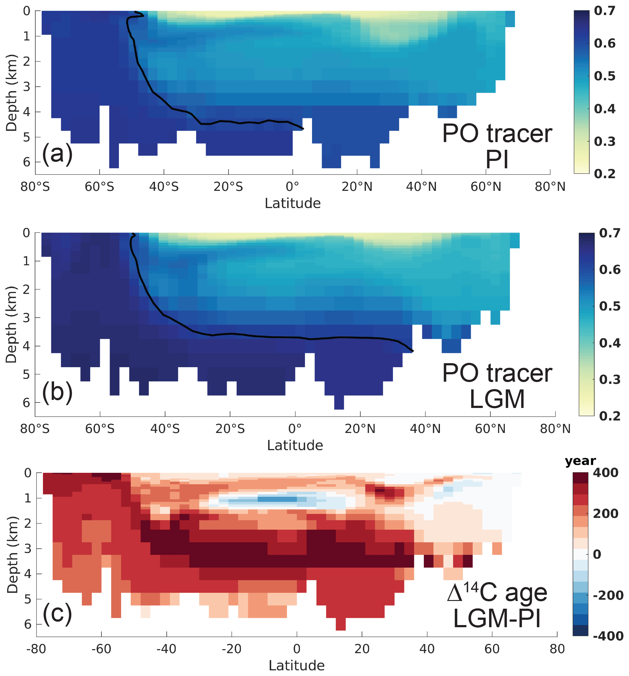
Figure 1Atlantic zonal mean of the conservative water mass tracer “PO” (25–35∘ W) for (a) the PI and (b) the LGM model states. (Broecker, 1974). The line represents the respective end-member PO of the Southern Source Water (mean Southern Ocean surface PO) and thus the extent of Southern Source Water. (c) The change in radiocarbon age between the LGM and PI. See Fig. S11 for the corresponding Pacific zonal mean transects.
It is important to note that can be changed by several processes: through the soft- and hard-tissue biological pumps, the solubility pump (Heinze et al., 1991; Volk and Hoffert, 1985), and changes in the physical carbon pump (circulation or stratification of the water column).
2.5 The Bern3D model
In order to put our offline calculations of the biological pump efficiency as applied to NorESM-OC (i.e., Sect. 2.4) in perspective, we performed an additional analysis using results from the Bern3D v2.0s intermediate complexity model. The Bern3D model includes a 3-D geostrophic frictional balance ocean (Edwards et al., 1998, Müller et al., 2006) coupled to a thermodynamic sea-ice component, a single-layer energy–moisture balance atmosphere (Ritz et al., 2011), and a 10-layer ocean sediment module (Tschumi et al., 2011). The Bern3D model components share the same horizontal resolution of 41×40 grid cells, and the ocean has 32 logarithmically spaced depth layers (Roth et al., 2014). A four-box representation of the land biosphere (Siegenthaler and Oeschger, 1987) is used to calculate the dilution of carbon isotopic perturbations. Further information on the Bern3D model is provided in the Supplement (Sect. S3). We used the Bern3D model to estimate the LGM–PI change in the marine DIC inventory (ΔDIC) in regard to changes in four observational targets (pCO2atm, δ13Catm, marine δ13C of DIC, and deep equatorial Pacific ), following the approach of Jeltsch-Thömmes et al. (2019). This is done by evaluating forcing–response relationships in seven generic carbon cycle mechanisms. These mechanisms are obtained from factorial deglacial simulations with the Bern3D model in a reduced form emulator – constrained by the observational targets. The seven generic forcings comprise changes in wind stress, air–sea gas exchange, the export rain ratio between organic and inorganic carbon, the remineralization depth of organic particles, coral growth, weathering of organic material, and carbon stocks in the land biosphere. More details on the experimental setup are given in Appendix A1. ΔDIC is estimated with this approach to be ∼3900 Gt C (±1σ range of [3350,4480] Gt C), based on the four given constraints. If only a single constraint of the four is applied, ΔDIC estimates are shifted by about 1000 Gt C towards lower values (see Appendix A2, Fig. A1). Contributions to ΔDIC from different carbon reservoirs that changed over the deglacial and eventually drew carbon from the ocean (atmosphere, land biosphere, coral reef regrowth, sedimentation–weathering imbalances) are discussed in Appendix A2.
The results presented in Sect. 3.1 and 3.2 are the annual mean climatologies over the last 30 years of the 5600-year PI and LGM spin-ups. The total integration time is long enough to eliminate most model drift at this point in time. Over the last 1000 years of the LGM spin-up simulation, ocean temperature does not show a significant trend, instead showing small oscillations with an amplitude of 0.015∘ (Fig. S4). SSS is stable for all practical purposes with a small positive trend of about 0.004 psu per 1000 years (Fig. S4). Likewise, AMOC strength is stable, while Drake Passage transport shows a small negative trend superimposed by variations in its strength of about 2 Sv (Fig. S5). We present an evaluation of the PI (Sect. 3.1) and LGM (Sect. 3.2) spin-ups, compare the latter to proxy reconstructions, and discuss the LGM–PI changes by exploring the efficiency of the biological pump (Sect. 3.3).
3.1 The simulated preindustrial ocean
The simulated preindustrial ocean state has a maximum AMOC strength of Sv north of 20∘ N, which compares favorably to the mean observational estimates of 17.2–18.7 Sv (Srokosz and Bryden, 2015; McCarthy et al., 2015), especially when noting the wide range of modeled AMOC strengths in similar forced ocean setups (Danabasoglu et al., 2014). The interannual variability of the simulated AMOC is small compared to observations (about ±4 Sv; Srokosz and Bryden, 2015), due to the annually repeating forcing. Drake Passage transport is simulated at ∼114 Sv, lower than recent observational estimate of 173.3±10.7 Sv (Donohue et al., 2016). The depth of the transition between the upper and lower Atlantic overturning cells at 30∘ S lies at ∼2700 m, comparable to other model estimates (Weber et al., 2007; Fig. S6). Temperature biases (Figs. S7a, b and S8a, b) are generally modest (smaller than ±1.5∘) for most of the ocean above 3000 m, except for a warm bias related to a too deep tropical and subtropical thermocline and a warm bias related to a too strong Mediterranean outflow at mid-depth in the Atlantic. At depth (>3000 m) there is a widespread cold bias that originates from the Southern Ocean (too much deep mixing and associated heat loss to the atmosphere). Salinity biases (Figs. S7c, d and S8c, d) are generally small, except for a positive bias related to the too strong Mediterranean outflow at mid-depth in the Atlantic. Furthermore, the ocean is ∼0.2–0.3 psu too fresh at depths over ∼3 km. The mixed-layer depth (MLD) is generally simulated too deep (compared to the observational estimates of De Boyer Montégut et al., 2004). In the high latitudes, winter month MLD biases in excess of 200 m are present in our model. In low latitudes, MLD is about 20 m too deep year-round. The simulated biogeochemistry of the PI ocean is described in more detail in Schwinger et al. (2016) although there have been some improvements due to the model updates mentioned above as described in Tjiputra et al. (2020). Some features of relevance for this study are summarized here: the spatial pattern of primary production (PP, Fig. S9) compares well with observation-based estimates with the exception of the tropical Pacific upwelling, where PP is too high, and the subtropical gyres and the coastal ocean where PP is generally too low. Because of too high PP and export in the equatorial Pacific, a far too large oxygen minimum zone (OMZ) with elevated concentrations of regenerated phosphate develops in the model (Fig. S10). Otherwise, the global nutrient concentrations are in reasonable agreement with modern observations (WOA, Glodapv2). is 38 % for the simulated PI ocean, in good agreement with observational estimates of 32 %–46 % (Ito and Follows, 2005; Primeau et al., 2013).
3.2 The simulated LGM ocean
3.2.1 The physical ocean state
Proxy-based reconstructions describe an LGM circulation that includes a shoaling of the upper circulation cell in the Atlantic (glacial North Atlantic Deep Water – NADW) and expansion and slow-down of a cooler and more saline lower circulation cell (glacial Antarctic Bottom Water – AABW; Adkins, 2013; Sigman et al., 2010; Ferrari et al., 2014). In this study, we assume these aspects of the LGM ocean to be qualitatively correct and therefore aim for a model simulation in agreement with these features. We note that discussion continues as to the magnitude and veracity of these changes (e.g., Gebbie, 2014). Most reconstructions estimate a weakened AMOC for the LGM as compared to the PI state, although estimates vary between a 50 % weakening and an invigoration of AMOC (McManus et al., 2004; Kurahashi-Nakamura et al., 2017; Böhm et al., 2014; Lynch-Stieglitz et al., 2007; Muglia et al., 2018). The maximum overturning strength north of 20∘ N simulated by NorESM-OC is 15.6 Sv (∼7 % weaker than simulated for our PI ocean, which we attribute to our adjustments and tuning of the salinity restoring). Higher uncertainties are involved with reconstructions of the strength of the Antarctic Circumpolar Current (ACC), with consensus leaning towards a slight invigoration (Lynch-Stieglitz et al., 2016; Lamy et al., 2015; McCave et al., 2013; Mazaud et al., 2010; Buchanan et al., 2016). We simulate a Drake Passage transport of 129 Sv (varying between ∼128 and ∼130 Sv, Fig. S5), which is about 13 % stronger than simulated for the PI ocean. The strengthening of the ACC in our simulation goes along with a strengthening in upwelling south of ∼55∘ S (not shown). The simulated transition between the Atlantic overturning cells shoals by ∼350 m (Fig. S6), which falls within the uncertainty of reconstructions (Gebbie, 2014; Adkins, 2013; Oppo et al., 2018) and is not captured in most PMIP simulations (Muglia and Schmittner, 2015). The transition between the overturning cells lies well above the main bathymetric features of the Atlantic Ocean in our LGM simulation (as visible in Fig. 1 from the transition line in the conservative PO water mass tracer). This could have been an important feature of the glacial Atlantic water mass configuration due to reduced mixing along topography (Adkins, 2013; Ferrari et al., 2014) – i.e., shifting water mass boundaries away from the regions of intense internal mixing increases chemical and tracer stratification. The changes in water mass circulation cause an increased SSW volume contribution to the Atlantic and Pacific basins, as visible from the conservative PO tracer (Figs. 1a, b and S11 for the Pacific) (Broecker, 1974) and in agreement with proxy reconstructions. Furthermore, the Atlantic abyssal cell is weaker in the LGM simulation as compared to the PI, which is important for the effects of the Southern Ocean on LGM pCO2atm drawdown (e.g., Kobayashi et al., 2015). Indeed, radiocarbon age increases at depth (Figs. 1c and S11 for the Pacific), with a global volume-weighted mean increase of 269 years. This is low compared to the estimate of Skinner et al. (2017) of 689±53 years, and we find the majority of our radiocarbon age bias to lie at depth in the Atlantic (not shown) indicating too strong ventilation and/or biased equilibration of these waters (which have a southern source, Fig. 1a, b). Our simulation shows a radiocarbon age increase particularly at mid-depth in the South Atlantic and South Pacific (at 2–3 km; Figs. 1c and S11). Burke et al. (2015) describe this “mid-depth radiocarbon bulge” as relating to the reorganization of the Atlantic overturning cell structure driven by Southern Ocean sea ice expansion. We simulate an increase in Southern Ocean sea ice cover for both summer and winter (Fig. S12), but it is less than is inferred from proxy-based reconstructions for the LGM (Gersonde et al., 2005) – similar to PMIP models (Roche et al., 2012). If the driving mechanism of the mid-depth radiocarbon bulge is indeed expanded sea ice as argued by Burke et al. (2015), improving our simulated LGM sea ice extent (Fig. S12) may increase (mid-depth) radiocarbon ages and improve agreement with proxy records like those of Skinner et al. (2017). Besides aging of SSW (Fig. 1c), the SSW salinity increases (Fig. S13), which is in good agreement with proxy reconstructions as well (Adkins, 2013). The simulated increased SSW salinity, radiocarbon age, and larger volume are important for simulation of LGM biogeochemistry and not a straightforward combination in glacial simulations (e.g., Kobayashi et al., 2015, PMIP). Nevertheless, our simulation of the LGM physical ocean state is most likely still not fully alike the LGM ocean (see also our discussion in Sect. 4). Also relevant for the water mass circulation, as well as marine biogeochemistry (Marzocchi and Jansen, 2019; Jansen, 2017), are the low LGM atmospheric temperatures that cause a mean ocean temperature decrease of 1.9 ∘C in the model. This is less than the 2.57±0.24 ∘C estimated from proxy reconstructions of mean ocean temperature (Bereiter et al., 2018), likely because the SSW may not carry a strong enough temperature decrease from the atmosphere into the interior ocean in our simulation (Fig. S14) – implying an underestimation of negative buoyancy fluxes. While the differences between our simulated LGM–PI changes in SST (Fig. S15) do not exhibit the same amount of heterogeneity as observed in proxy reconstructions (MARGO Project Members, 2009), the simulated mean SST change (−1.97 ∘C) seems reasonable when taking into account the uncertainty of SST reconstructions (MARGO Project Members, 2009 estimate ∘C; Ho and Laepple, 2015). Further, the general pattern of stronger SST cooling outside of the polar regions is captured, which is important for the air–sea disequilibrium pump (Khatiwala et al., 2019).
3.2.2 The biogeochemical ocean state
Proxies for the past biogeochemical state of the ocean (such as export production, oxygen concentrations, δ13C) allow us to make a further evaluation of our simulated LGM ocean (Fig. 2). The global mean efficiency of the biological pump decreases from 38 % in the PI simulation to 33 % in the LGM simulation, as opposed to reconstructions that infer an increased regenerated signature in the interior ocean (Jaccard et al., 2009; Umling et al., 2018; Freeman et al., 2016; Yamamoto et al., 2019). The simulated increase in preformed phosphate (Fig. 2) represents an increased (but unused) potential for the ocean to draw down pCO2atm (Ödalen et al., 2018). We can attribute our simulated decrease in to the increase in SSW volume (Fig. 1), as SSW has a low regenerated signature (Ito and Follows, 2005). Despite the decrease in , simulated pCO2atm is 20.3 ppm lower in our LGM setup as compared to the PI setup. We attribute this change to the net effect of the (i) smaller ocean volume, causing the concentration of alkalinity, DIC, and salinity and a reportedly ∼16 ppm pCO2atm increase (Sarmiento and Gruber, 2006), and (ii) the decrease in water temperature, which drives a pCO2atm drawdown of ∼30 ppm (Sigman and Boyle, 2000). As we made no additional changes to the marine biogeochemical model (except for the LGM dust input field) and have no sediment or land model included in our simulation, the ∼20 ppm pCO2atm drawdown, as well as limited changes in regenerated nutrient inventories, is expected and found in earlier studies (e.g., Buchanan et al., 2016). Physical processes thus mostly drive the simulated changes in pCO2atm and marine δ13C between our LGM–PI simulations, also evidenced by the LGM increase in preformed DIC (Fig. S16). The atmospheric and marine mean δ13C change due to glacial land–vegetation loss is not simulated because we only simulate the ocean. Simulated atmospheric δ13C remains approximately constant with a small increase of 0.07 ‰ from the PI (−7.46 ‰) to the LGM (−7.39 ‰). Mean marine δ13C increases 0.21 ‰ from 0.54 ‰ (PI) to 0.76 ‰ (LGM) at odds with the reconstructed LGM–PI 0.34±0.19 ‰ decrease reconstructed by, for example, Peterson et al. (2014), but this is partly expected in absence of a sediment or land model (see also the discussion in Sect. 4.4).
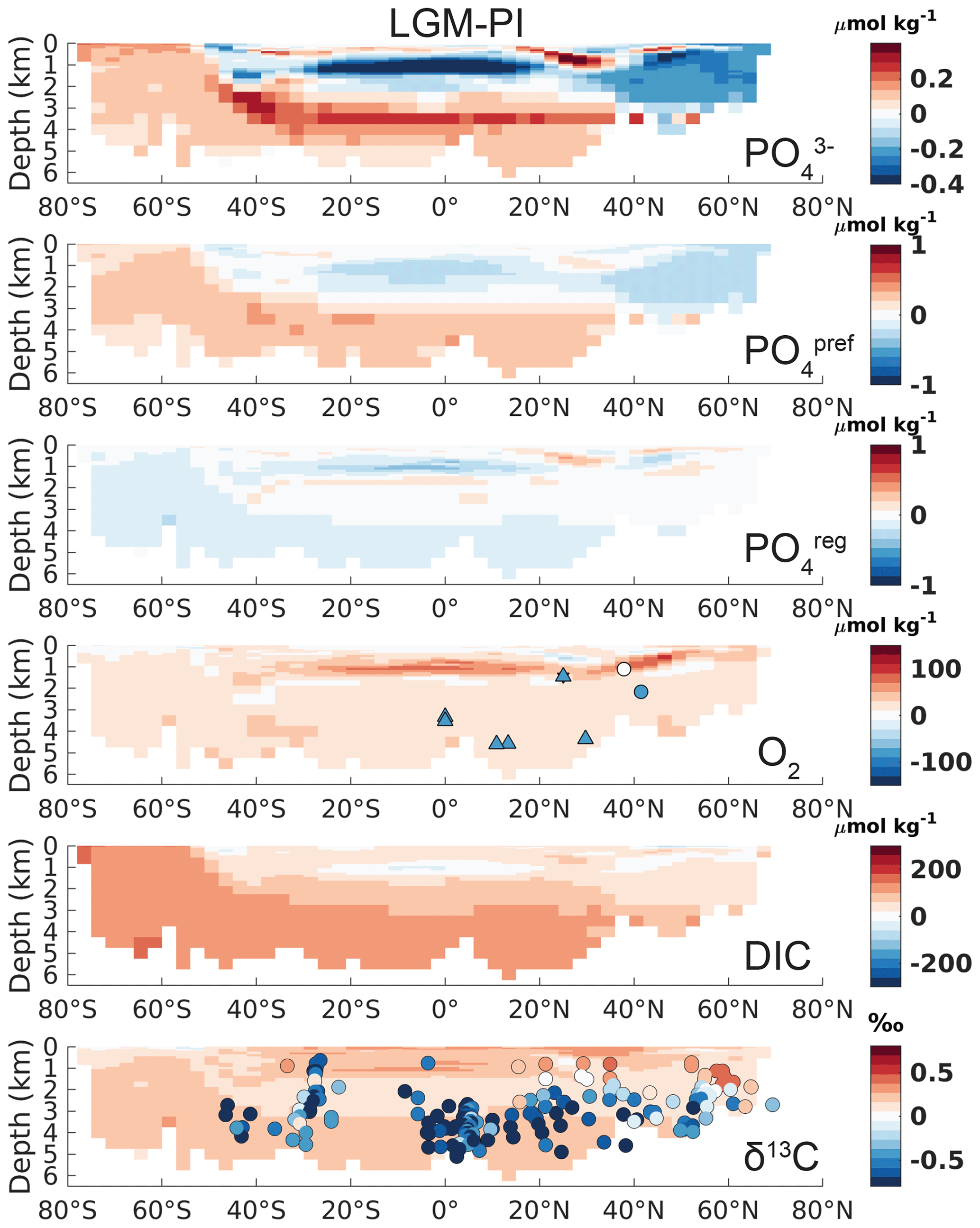
Figure 2Atlantic zonal mean (25–35∘ W) of LGM–PI changes for the original model output. See the left-hand column of Fig. S17 for the corresponding Pacific sections. Overlaid onto O2 are the qualitative estimates of LGM–PI changes in O2 within 30∘ from 30∘ W, with blue being a decrease, white indicating unclear changes, and red indicating an increase in O2 (Jaccard and Galbraith, 2011). Simulated LGM–PI δ13C is compared to a compilation of LGM minus Late Holocene δ13C data within 30∘ from 30∘ W (Peterson et al., 2014; Muglia et al., 2018; Molina-Kescher et al., 2016; Sikes et al., 2016; Burckel et al., 2016; Gottschalk et al., 2016b, c; Hodell and Channell, 2016; Howe and Piotrowski, 2017).
Simulated changes in Atlantic total phosphate (Fig. 2) agree well qualitatively with reconstructed nutrient redistributions, which describe a deep-ocean nutrient increase and mid-to-surface decrease (Buchanan et al., 2016; Gebbie, 2014; Marchitto and Broecker, 2006; Oppo et al., 2018). Northern Pacific waters >2.5 km depth exhibit a lower LGM phosphate (and DIC) compared to the PI, due to the lack of accumulated regenerated phosphate (Fig. S17). In agreement with the expectation of increased interior carbon storage, simulated interior DIC increases – especially in SSW (Fig. 2). As for phosphate, this increase is driven by the physical carbon pump only, through higher saturation of surface DIC in the Southern Ocean driven by lower T and increased alkalinity (see also Sect. 4 for a discussion on the contribution from the different DIC components).
However, the biases in simulated O2 and δ13C LGM–PI changes and their respective proxy reconstructions are large and in disagreement with proxy data (Fig. 2). Any mismatch in the absolute values of δ13C is not shown here because we compare LGM–PI differences in both the sediment cores and model. In line with decreased remineralization and increased O2 solubility due to lower temperatures in the model, O2 concentrations increase throughout the ocean (Fig. 2). There is a notable difference between northern and southern end-members in the Atlantic: Northern Source Waters have increased O2 concentrations due to physical O2 pumping (colder waters have higher O2 solubility), as is visible in preformed O2, while SSW O2 increases due to a lack of remineralization at depth due to low oxygen utilization (Fig. 3). As a final comparison, we evaluate our modeled changes in export production against proxy data, even though such data have poor global coverage and large spatial heterogeneity and are largely qualitative (Kohfeld et al., 2005). LGM export production generally decreases outside of upwelling zones in our model (Fig. 4) and increases in upwelling zones (model and proxy data, Fig. 4). We conclude that the simulated export production increase may be too weak in the sub-Antarctic and is lacking in the tropical Atlantic (Fig. 4).
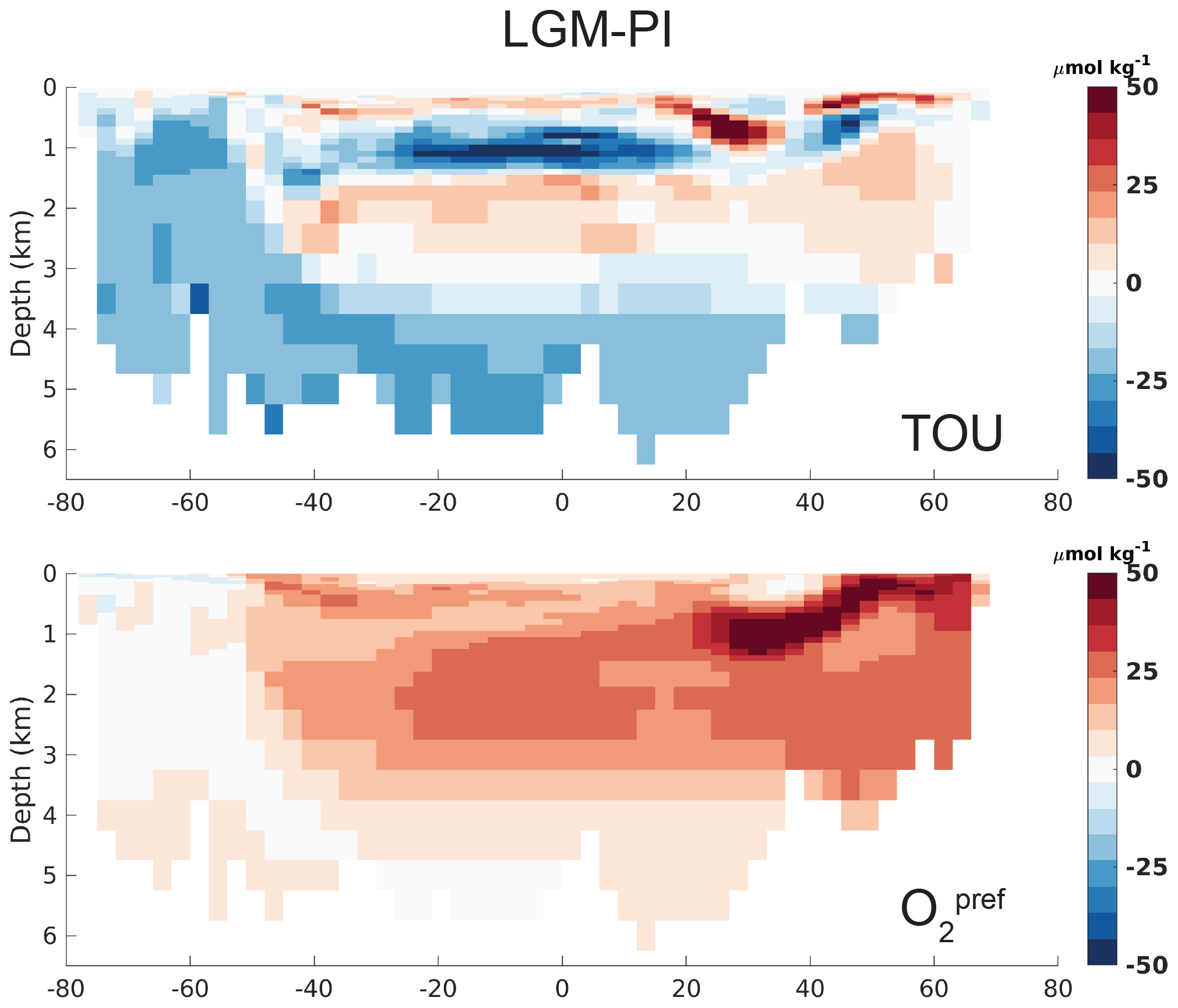
Figure 3Atlantic zonal mean (25–35∘ W) of simulated LGM–PI O2 component true oxygen utilization () (Ito et al., 2004) and preformed O2 (), which is simulated as the O2 concentration that leaves the surface ocean and is thus different from saturated O2 (Tjiputra et al., 2020).
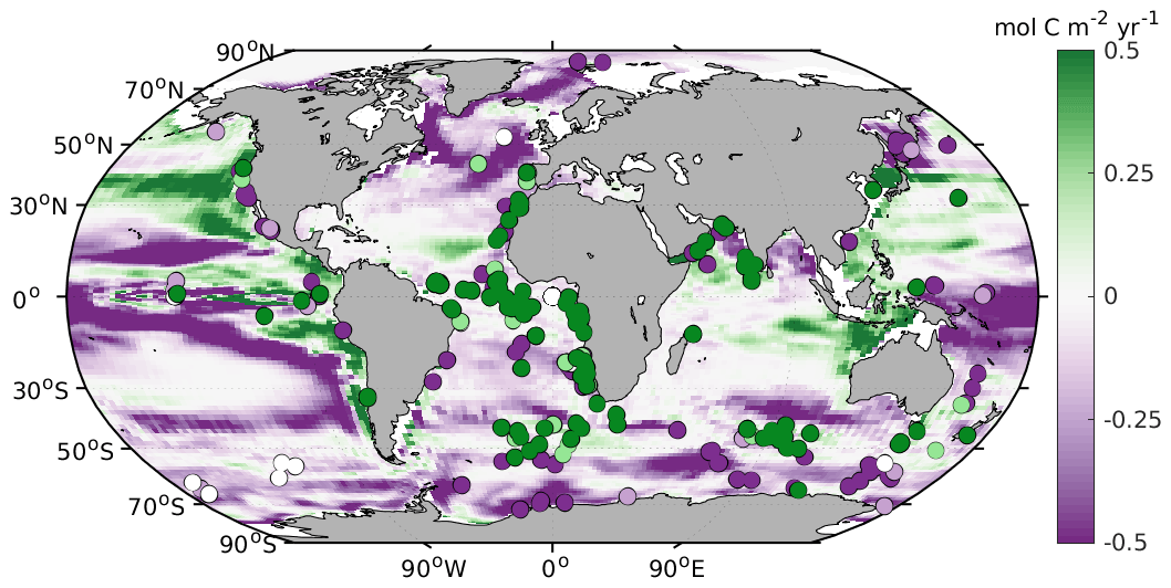
Figure 4Comparison between the simulated LGM–PI change in export production at 100 m depth and Kohfeld et al. (2005) qualitative data (dots: dark purple represents a decrease, light purple represents a small decrease, white represents no change, light green represents a light increase, and dark green represents an increase).
3.3 The potential of the biological pump
A decrease in pCO2atm and increase in regenerated nutrients, despite an increase in low regenerated nutrient SSW volume, is likely to occur through the increase of BPeff (and thus regenerated nutrients) of SSW (Jaccard et al., 2009). In addition, an increase in the (Southern Ocean) air–sea disequilibrium of DIC may have kept more carbon sequestered in the deep ocean through increased stratification and inhibition of air–sea gas exchange (Khatiwala et al., 2019) by, for example, sea ice (Marzocchi and Jansen, 2019). An increase in the regenerated signature of Northern Source Water would have further contributed to a global increase in regenerated carbon and nutrients in the interior ocean (Yu et al., 2019), although it would have occupied a smaller volume. As natural preformed concentrations in SSW are high (Ito and Follows, 2005), there is a high potential for these waters to obtain a stronger regenerated signature and thereby facilitate pCO2atm drawdown (Ödalen et al., 2018). Our model results for the LGM–PI change in O2 and δ13C show a strong mismatch with proxy records (Sect. 3.2.2 and Fig. 2). Here, we explore the effect of a potential increase of regenerated nutrients in the ocean by increasing regenerated phosphate and updating O2, DIC, and δ13C accordingly (Sect. 2.4). The increase is projected on the same simulated physical ocean state presumed to represent LGM conditions (i.e., Sect. 3.2.1). To the extent that this physical state represents true glacial conditions (see also the discussion in Sect. 4.1), it allows for an assessment of the magnitude and nature of marine biogeochemical changes needed for lowering LGM pCO2atm. In our approach, the additional regenerated phosphate is taken from preformed phosphate, thus leaving the total phosphate inventory unchanged. Proxy reconstructions of global LGM phosphate, however, show that LGM phosphate was redistributed as well as elevated (Tamburini and Föllmi, 2009; Filippelli et al., 2007). As we consider a closed system (no sediments or land input of phosphate or other elements), only redistributions of phosphate can be captured in our model setup.
We compare the mean error between the model and the δ13C proxy data across a wide range of (20 %–100 %, Fig. 5) and for the different methods of adding regenerated δ13C (Sect. 2.4). The best fit between the modeled and sediment core LGM–PI changes in δ13C is found for a of ∼75 % (Fig. 5). A of ∼75 % would lead to the adjusted tracer distributions shown in Fig. 6 (applying Eqs. 2–4). This is true for the approach “factor” (described in Sect. 2.4), indicating that taking the distribution of the original simulated LGM and strengthening that regenerated signal gives the best agreement with sediment core data. The of 75 % corresponds to an LGM–PI ΔDIC of ∼1850 Gt C. This ΔDIC estimate falls below the overall range (2400 to 5500 Gt C) given by the Bern3D model and its constraints (Sect. 2.5). If using only one of the Bern3D model constraints (pCO2atm, δ13Catm, marine δ13C of DIC, and deep equatorial Pacific ), however, the ΔDIC estimate of ∼1850 Gt C lies in the range of Bern3D results (see Appendix A for details). The estimated ΔDIC of ∼1850 Gt C allows for full (i.e., ∼80 ppm more than simulated, which is ∼170 Gt C) LGM pCO2atm drawdown, a profound decrease in land carbon (∼850 Gt C as estimated in Jeltsch-Thömmes et al., 2019), and a source of DIC from the deep ocean sediments/CaCO3. We can, however, not determine these sources and sinks in our model setup.
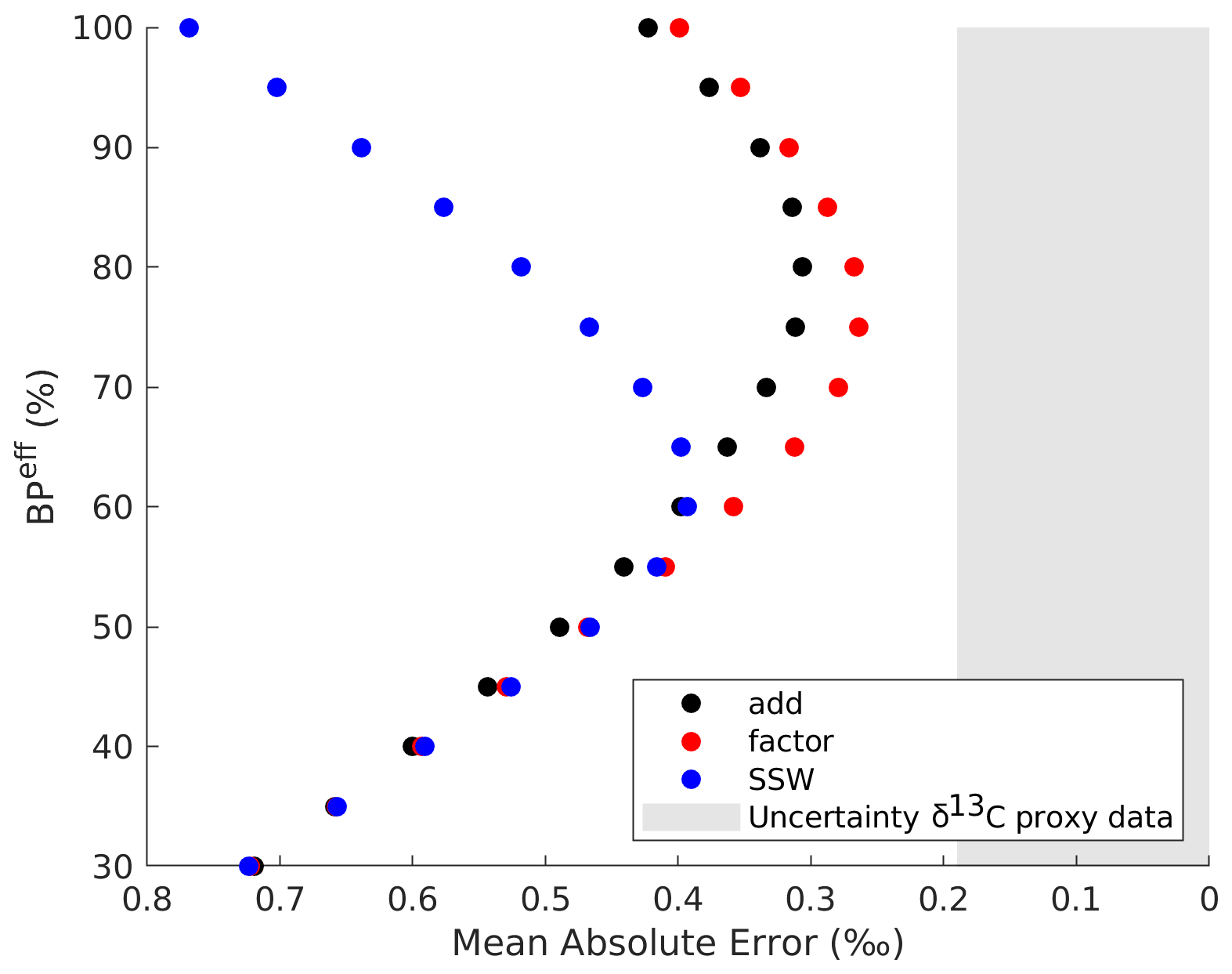
Figure 5Efficiency of the biological pump () versus the mean absolute error between all δ13C proxy data and the nearest model grid cell δ13C for different methods (Sect. 2.4). Note that the original LGM is 33 %. The δ13C sediment core data have an uncertainty of ∼0.19 ‰, which is shaded in grey (Peterson et al., 2014).
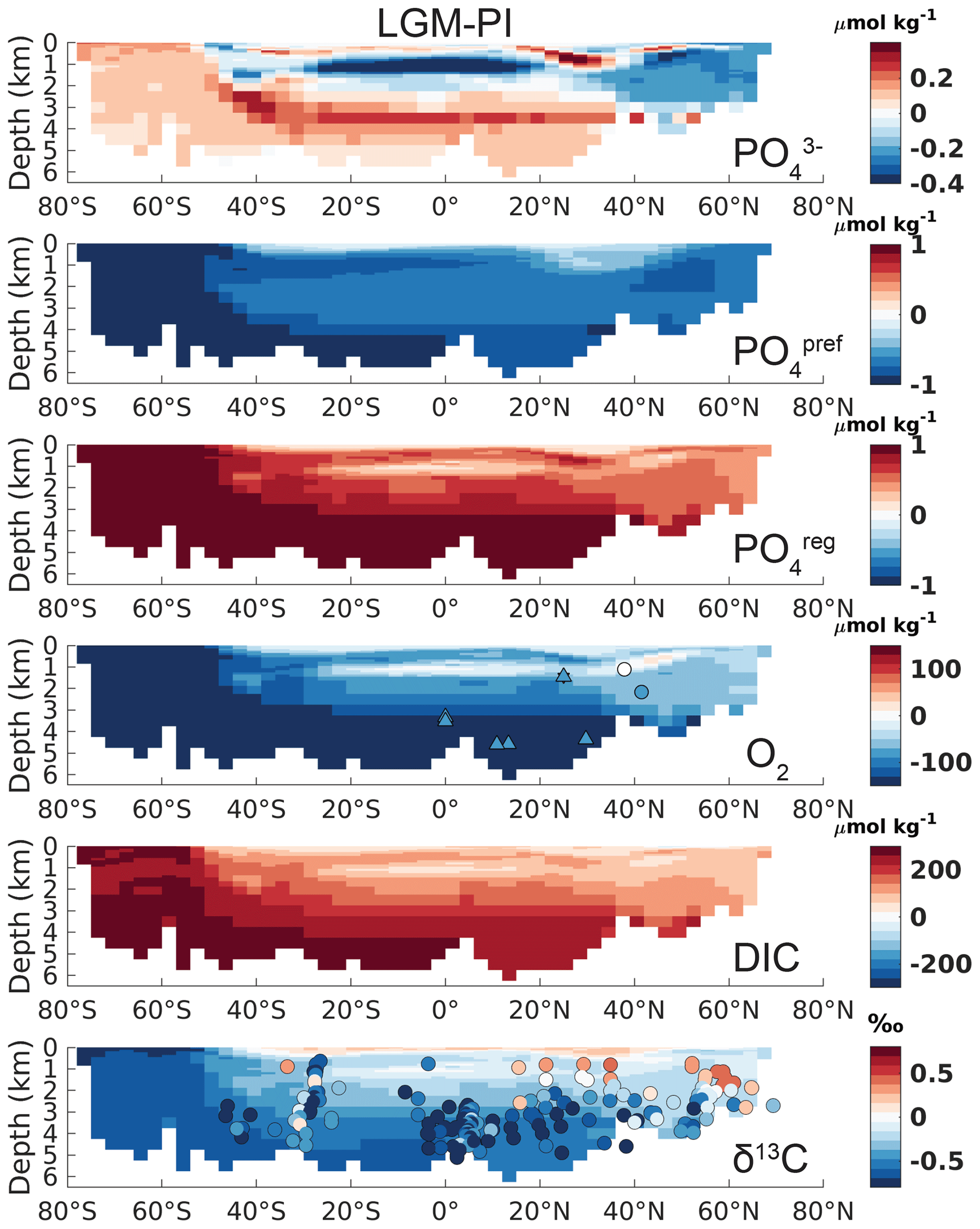
Figure 6The same as Fig. 2 but for an adjusted of 75 %. See the right-hand column of Fig. S17 for the Pacific transects.
In addition to evaluating the model–data fit of δ13C, we evaluate the effect of the tracer adjustments on O2. The decrease in O2 for an adjusted (Fig. 6) shows better agreement with qualitative proxy data in the Atlantic (compare Figs. 2 and 6; Jaccard and Galbraith, 2011), as well as the estimated 175±20 µmol kg−1 LGM–PI decrease in sub-Antarctic Atlantic Bottom Water (Gottschalk et al., 2016a). Absolute LGM O2 (Fig. S18) would decrease to sub-zero O2 concentrations in the northern Pacific (ca. −100 µmol kg−1). This is of a similar magnitude as the size of the PI model–observation bias in this area (Tjiputra et al., 2020) but may be too extreme, as indicated by qualitative proxy data that describe an LGM–PI O2 increase for the northern Pacific above 3 km depth (Fig. S17; Jaccard and Galbraith, 2011). An increase in denitrification could have played a role here but cannot be evaluated in our model setup. Additional (quantitative) estimates of LGM–PI O2 for major water masses would thus help to provide further constraints on LGM .
Our mean absolute error in δ13C decreases from 0.67 ‰ for the original LGM state estimate (Fig. 2) to 0.26 ‰ for the 75 % ocean (Figs. 5 and 6). The remaining absolute δ13C error is therefore 0.07 ‰ larger than the proxy data uncertainty. After adjustment of to 75 %, the remaining mean model–data δ13C mismatch of 0.07 ‰ (Fig. 5) as well as the possibly too low Pacific O2 (Fig. S18) indicate that projecting changes in onto the simulated glacial circulation field still does not fully align with the actual LGM state – despite exploring different approaches for the redistribution of the regenerated nutrients (Sect. 2.4). In Sect. 4.4 we discuss possible mechanisms that could contribute to understand this remaining mismatch.
Earth system models are generally found to incompletely capture the biogeochemistry and strengthening of the biological pump for the LGM ocean, and identification of the exact processes that are missing in these models is a major challenge in modeling the LGM ocean (e.g., Galbraith and Skinner, 2020). Previous studies show that both physical and biological marine changes must have contributed to the LGM pCO2atm drawdown (Bouttes et al., 2011; Buchanan et al., 2016; Khatiwala et al., 2019; Yamamoto et al., 2019; Kobayashi et al., 2015; Stein et al., 2020; Marzocchi and Jansen, 2019). The physical ocean state of our LGM simulation compares quite well to proxy data (Sect. 3.2.1), while the simulated biogeochemical state (Sect. 3.2.2) reveals major disagreements with proxy data and a too weak LGM . Nevertheless, our modeled can be increased through both physical and biological mechanisms.
Previous studies on LGM model–data comparisons employing δ13C of DIC reveal that a change in ocean circulation is mandatory in explaining the change in global ocean δ13C pattern with respect to the late Holocene and preindustrial (Heinze et al., 1991; Winguth et al., 1999; Crucifix, 2005; Tagliabue et al., 2009; Hesse et al., 2011; Gebbie, 2014; Schmittner and Somes, 2016; Menviel et al., 2017; Muglia et al., 2018; Menviel et al., 2020). Some of the model simulations can achieve a fairly good fit to δ13C from the LGM sedimentary δ13C archive by varying the oceanic forcing and the ocean circulation alone (e.g., Winguth et al., 1999; Hesse et al., 2011, Gebbie, 2014; Menviel et al., 2017). However, there is no convincing case where, based on circulation changes alone, a quantitatively correct drawdown of atmospheric pCO2 could be explained. This dilemma had been addressed in Tagliabue et al. (2009) through stating that ocean circulation changes can explain a large part of the δ13C signal in the ocean but not the atmospheric pCO2 drawdown. The latter may require further processes – in addition to ocean circulation changes – such as an ecologically or biogeochemically induced vertical redistribution of nutrients and carbon as addressed in this study here. This viewpoint is corroborated by multi-tracer–multi-parameter studies (e.g., Heinze and Hasselmann, 1993; Brovkin et al., 2007; Heinze et al., 2016).
4.1 Physical model–data biases of the LGM simulation
To start, our results may indicate that the water mass production processes in the model are not (yet) fully adequate and contribute to the too low simulated LGM and too weak chemocline. Interior δ13C is influenced by the source of deep waters and intermediate waters, the extent of deep convection, and mixing processes between interior water masses (e.g., Duplessy et al., 1988), partly on spatial and temporal scales possibly not resolved by our model. An example is the role of shelf processes and the related localized sea ice formation and brine excretion in the Southern Ocean, which are highly relevant for SSW characteristics and the transition between the overturning cells (Klockmann et al., 2016; Mariotti et al., 2016; Bouttes et al., 2011; Jansen, 2017; Marzocchi and Jansen, 2017; Stein et al., 2020). The PI simulation of a generally too deep Southern Ocean mixed-layer depth, as well as Southern Ocean-attributed model biases in the PI biogeochemical tracers (Sect. 3.1; Tjiputra et al., 2020), suggests that deep-water formation processes are indeed not simulated in full agreement with observational data – which may lead to biases in the LGM simulation as well. Furthermore, the lack of a reliable glacial freshwater forcing is likely to be partly responsible for biases in the LGM simulation. The weak LGM–PI reduction of SSW temperature (Fig. S14) is in disagreement with proxy records and implies an underestimation of negative buoyancy fluxes. Improving this bias may, however, lead to more vigorous sinking of SSW in the Southern Ocean and possible speed-up of the abyssal overturning cell, equally in disagreement with proxy data. Additionally, too strong exchange (mixing) in the LGM ocean between the deep and intermediate waters could contribute to maintaining a too weak glacial chemocline. Our simulated SSW radiocarbon ages are too young compared to reconstructions (Fig. 1), consistent with inadequate isolation of these waters in the simulation. Further aging of these SSW could increase their regenerated signature (consuming O2 and decreasing δ13C of DIC) and steepen the chemocline while additionally improving agreement with the Bern3D model ΔDIC estimate and radiocarbon age. Indeed, both increased stratification and enhanced biological pumping in the glacial Southern Ocean likely played a role in deoxygenating SSW (Yamamoto et al., 2019).
Several key physical processes may be central to improving our model biases: (i) polar wind stress forcing, related to the ice sheets (e.g., Muglia and Schmittner, 2015; Galbraith and Lavergne, 2019), (ii) polar sea surface salinity forcing (this study, Rahmstorf, 1996; Spence et al., 2008; Bopp et al., 2017; Weber et al., 2007), and (iii) Southern Ocean sea ice cover. The simulation of a larger increase in LGM Southern Ocean sea ice extent (Fig. S12) and/or formation rate may lead to a more stratified and isolated SSW (Ferrari et al., 2014; Nadeau et al., 2019; Jansen, 2017; Marzocchi and Jansen, 2017, 2019; Stephens and Keeling, 2000; Stein et al., 2020). This could create older waters with higher regenerated signatures and increase the air–sea disequilibrium of biogeochemical tracers such as DIC and O2 (Gottschalk et al., 2016a; Khatiwala et al., 2019; Yamamoto et al., 2019), thereby further lowering atmospheric CO2 (Khatiwala et al., 2019) and increasing SSW radiocarbon aging.
4.2 Biogeochemical model–data biases of the LGM simulation
Regarding biological mechanisms that could underlie our model bias, it is instructive to first look at our simulation of a simultaneous decrease in and pCO2atm (Sects. 3.2 and 4.1). This apparent contradictive result can be attributed to the fact that our model mostly captures the physical carbon pump, as driven by temperature and ocean volume decrease. Indeed, decomposition of DIC into its components (DICsoft, DICpref, DICsat, DICbio, DICcarb, and DICdiss: Fig. S16; Bernardello et al., 2014) shows that the increased ocean inventory of DIC (which is driving down pCO2atm) can be attributed to the increase in the physical DICpref component. Specifically, DICpref increases due to increased DIC disequilibrium (DICdiss) of SSW with the atmosphere and a strengthened solubility pump, as evidenced by increased DICsat. The more isolated abyssal cell (and accompanying increase in DICdiss) is central for the lower glacial pCO2atm, as described throughout this paper. Nevertheless, our study shows that the increased DICdiss is not sufficient for the simulation of a full glacial pCO2atm drawdown and that additional changes in the biological carbon pump must have played a role. In our simulation, DICsoft lowers the ocean inventory of DIC in line with the simulated decrease in but in disagreement with proxy records.
The lack of an increased marine C inventory through the increase in DICsoft is also evident from simulated O2 and δ13C. In our simulation, O2 concentrations increase due to the lack of biological O2 consumption at depth in SSW and increased solubility in Northern Source Waters (Fig. 3). Such an O2 increase is in disagreement with proxy reconstructions (Jaccard and Galbraith, 2011) and argues for biological processes to explain the missing regenerated nutrients (i.e., remineralization) and low DICsoft in our simulation. As for O2, the widespread increase in simulated δ13C of DIC contradicts δ13C records from sediment cores, in which the strengthening of the vertical gradient is a main feature (Fig. 2). Importantly, deep δ13C and its vertical gradient is partly governed by biological processes (Morée et al., 2018), further arguing for biological processes to contribute to our simulated biases. Nevertheless, δ13C of DIC is governed by both ocean circulation (ventilation rate) and the efficiency of the biological pump (respiration rate), and their relative importance depends on their location in complex and highly spatially heterogeneous ways (Gruber et al., 1999; Schmittner et al., 2013; Eide et al., 2017; Morée et al., 2018). A possible candidate to increase deep DICsoft is found in Southern Ocean export production, which has a great potential to affect interior and lower-latitude nutrient and DIC concentrations (Sarmiento et al., 2004; Primeau et al., 2013). Iron fertilization likely played a central role in the increase in production and export fluxes as well (e.g., Winckler et al., 2016; Costa et al., 2016; Oka et al., 2011; Lambert et al., 2015; Yamamoto et al., 2019) and may be insufficiently captured by our model. Comparison between our simulation and proxy data point to an underestimation of LGM export production in the ice-free Southern Ocean (Fig. 4), which we conclude may have contributed to the simulated low and low regenerated signature in the biogeochemical tracer distributions. The biological pump efficiency and hence the Δδ13C further depend on the details of the particle flux mode through the water column. This flux depends on the size of the sinking particles, their composition, aggregation, and weight. The plankton community structure plays an important role here (Bach et al., 2019). The vertical particle flux can be accelerated, e.g., through enhanced dust deposition (clay), biogenic opal, and calcium carbonate (Haake and Ittekkot, 1990; Armstrong et al., 2001; Klaas and Archer, 2002; Honda and Watanabe, 2010; Mendes and Thomsen, 2012). The production of transparent exopolymer particles (TEP) also modifies the vertical flux mode of organic matter substantially (De La Rocha and Passow, 2007; Mari et al., 2017). These details of marine particle fluxes still need to be accounted for in marine biogeochemical models and can have differential effects on the regional biological pump efficiency. Finally, we note that many of the biogeochemical processes mentioned here are closely related to ocean circulation. Therefore, changes in LGM–PI water mass configuration and overturning strength beyond those captured by our model are strong candidates for reducing model–proxy data biases.
4.3 Other sources of model–data bias of the LGM simulation
Besides alleviating model biases in physical or biological processes, our simulation of the LGM ocean may be improved through model development: for example, the results of our simulations on pCO2atm may be amplified through carbonate compensation in interplay with Southern Ocean stratification (Kobayashi and Oka, 2018) if we also included the ocean sediments in our simulations. The latter would also facilitate direct comparison with sediment core records, especially if the carbon isotopes are included in the sediment model. In addition, changes in the CaCO3 counter pump provide a “wild card” for adding to the atmospheric pCO2 reduction with only negligible influence on the oceanic δ13C distribution. In order to reduce the uncertainties in ocean forcing during glacial times, it is vital to narrow down the freshwater flux uncertainties, e.g., through data assimilation methods. Finally, a decreased δ13C of DIC is possible without drastic increases in regenerated nutrients when considering changes in C:P ratios (Ödalen et al., 2020). Such C:P changes could contribute to resolve the model–proxy error and provide an interesting direction for future work.
Despite the possible shortcomings of our simulation discussed here, our simulation of a salinity increase (Fig. S13), a slowdown (Fig. S6), cooling (Fig. S14), increased volume (Fig. 1a, b), and aging (Figs. S11, 1c) of the abyssal overturning cell combined with reduced pCO2atm are rarely obtained (compare to, e.g., Kobayashi et al., 2015; Weber et al., 2007; Muglia and Schmittner, 2015; Sigman et al., 2010; Klockmann et al., 2016).
4.4 The remaining model–data bias after adjustment
Changes between preindustrial and LGM ocean circulation fields as simulated by ocean models generally fail to account for the full 100–120 ppm drawdown in atmospheric CO2 (taken the outgassing by the land biosphere into account) when used in global ocean carbon cycle models (Heinze et al., 1991; Brovkin et al., 2007). Indeed, our study gives an estimate of ∼20 ppm drawdown with an unadjusted biological pump efficiency.
The adjustment of the to 75 % in addition to the reorganized circulation captures most of the magnitude of the LGM–PI δ13C change (Figs. 5, 6 and S17). However, the strength of the glacial chemocline (the vertical δ13C gradient) remains too weak (Fig. 6). Other modeling studies of the glacial ocean show similar biases (e.g., Heinze et al., 2016; Schmittner and Somes, 2016). This suggests that additional processes, which would allow stronger chemical stratification between intermediate and deep waters, are missing in the model(s) and are not explained in a simple way by intensification of the (soft-tissue) biological pump or our simulated changes in circulation. We recognize that optimizing the model to additional (quantitative) proxies such as the nitrogen isotopes could provide more constraints (Schmittner and Somes, 2016). Aside from this, our offline calculations to increase the biological pump efficiency may be too simplified to capture the vertical redistribution of regenerated nutrients, which is also suggested by the too weak chemocline.
Using their idealized model setup, Schmittner and Somes (2016) estimated an LGM of 54 %–59 % (41 % in PI) and a ΔDIC of 590–790 Gt C by exploring the effects of a uniform change in the maximum growth rate of phytoplankton. A direct comparison between these studies is complicated by the large differences between the models, but the differences indicate remaining uncertainties in the magnitude of both ΔDIC and LGM . Nevertheless, LGM seems to have been about 18 (i.e., 59–41) % and up to 37 (i.e., 75–38) % higher than in the PI. Finally, we note that the total marine ΔDIC (∼1850 Gt C) estimate points towards a central role of the Pacific basin in storing glacial carbon, if we consider Atlantic LGM storage >3 km depth to be on the order of 50 Gt C (Yu et al., 2016).
Finally, we wish to make an estimate of the effect of land biosphere and sedimentation–weathering imbalances on our analysis. The net excess transfer of light 12C to the ocean during the LGM is estimated in the Bern3D model to cause a relatively uniform ∼0.4 ‰ decrease in LGM mean marine δ13C as compared to the PI ocean for a 890 Gt C change in land biosphere carbon, along with a similar −0.4 ‰ shift in δ13Catm (Jeltsch-Thömmes et al., 2019). The proxy-based mean marine LGM–PI δ13C shift of 0.34±0.19 ‰ (Peterson et al., 2014) constitutes the combined effect of land biosphere, atmospheric, and sedimentation–weathering imbalances, in addition to a strengthening of the δ13C gradient (the latter of which represents a low deep-ocean δ13C, thereby lowering mean marine LGM δ13C through its large volume). We provide an estimate of the potential effect of a shift in mean marine δ13C on our analysis: if we choose to make a uniform correction to the simulated LGM δ13C of −0.4 ‰ (such that mean marine δ13C LGM–PI ‰ in our model) before comparing to proxy data, Fig. 5 looks like what is shown in Fig. S19a. In this case, adjusted with the lowest mean absolute error is ∼55 % and corresponds to a ΔDIC of ∼1000 Gt C. If we make a smaller mean shift of −0.2 ‰, we obtain a best fit for of ∼65 % and a ΔDIC of ∼1425 Gt C (Fig. S19b). We note, however, that such mean shifts in marine δ13C would also affect δ13Catm, thus calling for the consideration of additional processes in order to fulfill the observational constraints in δ13C in the ocean and atmosphere simultaneously (see also the discussion in Jeltsch-Thömmes et al., 2019). To our knowledge, no consensus exists on the relative importance of the different drivers on LGM–PI shifts in mean marine δ13C due to the large uncertainties of the LGM–PI changes in the relevant carbon reservoirs (as illustrated for the Bern3D model in Fig. A1b). We therefore limit ourselves to quantifying the potential effects of such a shift on our analysis.
We present a model simulation of the preindustrial and Last Glacial Maximum (LGM) oceans. We use the simulations to explore a realization of physical and biological marine changes needed to simulate an LGM ocean in satisfactory agreement with proxy data. Despite the good agreement between (qualitative and quantitative) proxy reconstructions and our simulation of different LGM and preindustrial (PI) ocean circulation, our model is unable to simulate the complete set of biogeochemical changes implied by proxy data. Therefore, our results (mainly the lack of increased regenerated nutrients) confirm the idea that both biogeochemical (beyond those represented by the model) and physical changes must have been at play in the ocean to create the LGM pCO2atm drawdown (Heinze et al., 2016; Bouttes et al., 2011; Buchanan et al., 2016). Comparison between a range of qualitative and quantitative proxy data and simulated biogeochemical tracers (specifically total dissolved inorganic carbon, regenerated phosphate, true oxygen utilization, O2, and δ13C) reveals that there is a too small signature of regenerated nutrients in our simulated LGM ocean. We conduct offline calculations of changes in the global mean efficiency of the biological pump and quantify its effect on the global mean absolute error between simulated δ13C and proxy δ13C data. The smallest error is found for an approximate doubling in the global mean efficiency of the biological pump (from 38 % in the PI ocean to ∼75 % in the LGM), when omitting the influence from land biosphere and sedimentation–weathering imbalances on mean marine δ13C from our analysis. This approximate doubling is likely driven by a combination of additional biological and physical changes, such as stronger isolation of SSW (as discussed in detail in Sect. 4.1 and 4.2). A of ∼75 % reduces the simulated global mean absolute error for δ13C from 0.67 ‰ (for the original simulated 33 % of the LGM) to 0.26 ‰ – only distinguishable by 0.07 ‰ from the δ13C data uncertainty. It additionally improves the agreement with both qualitative and quantitative O2 reconstructions.
A mean shift of marine LGM δ13C due to sedimentation–weathering imbalances and land biosphere release of low δ13C can affect our analysis (Fig. S19). Our ocean model does not capture such a shift since we omit the land biosphere and sediments. Since quantification of the contribution of different mechanisms to the shift in mean marine δ13C is still under debate, we limit ourselves to quantifying the potential effect of a mean shift in marine δ13C on our analysis: a uniform marine shift of −0.2 ‰ and −0.4 ‰ is made to our LGM simulation to estimate the effect on our analysis of . In these cases, the best-fit LGM lies closer to ∼65 % and ∼55 %, respectively (Fig. S19). We conclude that our analysis, which omits mean shifts in marine δ13C due to sediment–weathering imbalances or land biosphere changes, provides an upper estimate of LGM . Future work could explore how changes in δ13Catm and sedimentation–weathering imbalances could affect marine δ13C in NorESM-OC.
Much of the remaining model–proxy δ13C data mismatch is due to a too weak vertical chemocline in glacial simulations. Therefore, scaling of the biological pump efficiency does not fully explain the glacial ocean proxy data using the modeled circulation field thought to most closely represent the glacial state. We see different explanations of the bias that could strengthen the glacial chemocline, such as the further aging (by isolation and stratification) of interior waters through improved simulation of deep-water formation, which would increase the regenerated signature of the interior LGM ocean. Southern Source Waters would have an especially large potential (due to their large volume contribution) to increase global interior radiocarbon ages and regenerated signatures of the interior ocean.
The estimated increase to 75 % corresponds to an increase in oceanic DIC (ΔDIC) of ∼1850 Gt C. This lies in the range of estimates as derived by the Bern3D Earth System Model of Intermediate Complexity constrained by single-proxy targets (pCO2atm, δ13Catm, marine δ13C of DIC, or deep equatorial Pacific ). If all four targets are used as constraints, the range of ΔDIC estimates based on the Bern3D model is higher than 1850 Gt C (see Fig. A1 and Appendix A2). In order to disentangle and understand the processes contributing to ΔDIC, especially the large contribution from sedimentation–weathering imbalances, further work seems necessary.
Our results underline that only those coupled climate models that contain processes and/or components that realistically change both ocean circulation and biogeochemistry will be able to simulate an LGM ocean in satisfactory agreement with proxy data. Such a simulation is also a test of Earth system models for their ability to reproduce natural climate variations adequately as a basis for reliable future projections, including human-induced forcing (e.g., Zhu et al., 2021); i.e., a satisfactory fidelity of Earth system models in reproducing orbitally forced climate variations will increase our confidence in these models as tools for projecting future anthropogenic climate change. Therefore, future research should aim to identify the exact physical and biogeochemical processes that could have driven the increase in global mean biological pump efficiency (i.e., the interior regenerated signature) between the PI and LGM, with a likely central role for Southern Source Waters.
The general agreement between our model results and proxy data for ocean circulation (within the uncertainty of reconstructions), after adjustments to the sea surface salinity field, demonstrates an advantage of our forced ocean model setup and its flexibility over fully coupled Earth system models in exploring different circulation and biological pump scenarios for explaining glacial CO2 changes. We conclude that a large PI-to-LGM increase in the efficiency of the biological pump (from 38 to up to ∼75 %), as well as a reorganization of ocean circulation and stratification, are essential for simulating an LGM ocean in optimal agreement with proxy data.
A1 Experimental setup of the Bern3D model
We estimate the LGM–PI change in marine DIC content (ΔDIC) by applying a reduced form emulator based on forcing–response relationships obtained from factorial simulation over the deglacial with the Bern3D model (see Jeltsch-Thömmes et al., 2019). The mean over 21 to 19 ka BP and over 500 to 200 years BP are used as LGM and PI time intervals for the calculation of ΔDIC. To estimate ΔDIC, the forcing–response relationships of seven generic deglacial carbon cycle mechanisms in regard to LGM–PI changes in four observational targets (pCO2atm, δ13Catm, marine δ13C of DIC, and deep equatorial Pacific ) and DIC are investigated with the Bern3D. The seven generic forcings comprise changes in wind stress, air–sea gas exchange, the export rain ratio between organic and inorganic carbon, the remineralization depth of organic particles, coral growth, weathering of organic material, and carbon stocks in the land biosphere. These seven generic deglacial carbon cycle mechanisms were varied individually by systematic parameter variations in addition to well-established forcings such as orbital parameters, greenhouse gas radiative forcing, land ice albedo, coral reef regrowth, and North Atlantic freshwater forcing. In a next step, Latin hypercube parameter sampling was used to vary the processes in combination, probe for nonlinear interactions, and use the results to adjust the above forcing–response relationships. An emulator of the form
is derived from the forcing–response relationships. is the sensitivity for each target T to the change in each mechanism Δpi. aT is the offset and bT the slope of the respective linear fit from the multi-parameter adjustment in order to correct for nonlinearities stemming from the addition of the seven generic mechanisms. We use the same half a million parameter combinations as Jeltsch-Thömmes et al. (2019) and investigate ΔDIC. The four proxy targets (pCO2atm, δ13Catm, marine δ13C of DIC, and deep equatorial Pacific ) are used as constraints.
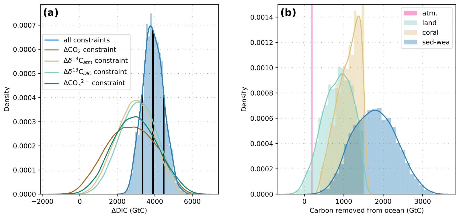
Figure A1(a) Histogram (blue bars, normalized) and kernel density estimate (blue line, all constraints) of ΔDIC (Δ is taken here as LGM minus PI) of parameter combinations fulfilling all four proxy constraints. Black vertical lines show the median ΔDIC estimate of ∼3900 Gt C and the ±1σ range of [3350,4480] Gt C. The other four lines are kernel density estimates of ΔDIC for parameter combinations fulfilling only one of the four proxy constraints at a time. (b) Contributions to ΔDIC (all four proxy constraints fulfilled) from the atmosphere, land, corals, and sedimentation–weathering imbalances.
A2 Results from the Bern3D model
Applying single constraints only yields similar ranges for ΔDIC for each constraint, covering the range of ΔDIC values from about 0 to 6000 Gt C (Fig. A1). Considering all four proxy targets simultaneously shifts the estimate of ΔDIC to higher values such that the covered range amounts to about 2400 to 5500 Gt C and a median estimate of about 3900 Gt C (±1σ range of [3350,4480] Gt C; Fig. A1). This might seem large at first. Considering changes in the different carbon reservoirs that changed over the deglacial and eventually drew carbon from the ocean (atmosphere, land biosphere, coral reef regrowth, sedimentation–weathering imbalances) helps to put the estimated ΔDIC into context (Fig. A1). The atmospheric increase over the deglacial is well constrained from ice cores and amounts to about 200 Gt C. The change in the land biosphere carbon storage is more uncertain. A recent estimate, which integrates multiple proxy data sources, derives an increase of the land biosphere over the deglacial of about 850 Gt C (median estimate) (Jeltsch-Thömmes et al., 2019), in good accordance with another recent estimate based on a dynamic global vegetation model (Müller and Joos, 2020). The growth of coral reefs during sea level rise removed an additional 380 Gt C (Vecsei and Berger, 2004) to 1200 Gt C and more (Milliman, 1993; Kleypas, 1997; Ridgwell et al., 2003) from the ocean. Imbalances in the sedimentation–weathering cycle of carbon need to be considered on the multi-millennial timescales. The contribution from sedimentation–weathering imbalances to ΔDIC is uncertain and ranges from a removal of almost 0 Gt C to more than 3000 Gt C from the ocean as estimated with the Bern3D model. The results thus point to an important role and large contribution from sedimentation–weathering imbalances to ΔDIC estimates over glacial–interglacial timescales but with a large uncertainty. Finally, it has to be noted that in order to use the cost-efficient emulator and explore a large parameter space, only the change between LGM and PI was considered. Including the spatiotemporal evolution of several proxies in transient model simulations will help to gain further understanding of governing processes and narrow down the ΔDIC estimate but is beyond the scope of this paper.
The model output data for the last 30 years of the PI (https://doi.org/10.11582/2020.00061, Morée et al., 2020a) and LGM (https://doi.org/10.11582/2020.00062, Morée et al., 2020b) simulations are freely available at the NIRD Research Data Archive. The LGM ocean simulation was forced from the atmosphere using the PMIP3-based atmospheric LGM-PI anomalies of Morée and Schwinger (2019, version 1).
The supplement related to this article is available online at: https://doi.org/10.5194/cp-17-753-2021-supplement.
ALM, JS, and CH conceptualized the study and developed the methodology in cooperation with IB and with contributions from AJT. ALM did the formal analysis of the data and wrote the original draft for which she visualized the results. ALM, JS, CH, AJT, and UN investigated the results. All authors contributed to the review and editing of the original draft. JS and ALM curated the data, contributed to the software, and validated the results. CH and JS supervised the project and provided the resources and funding acquisition needed for this work.
The authors declare that they have no conflict of interest.
This article reflects only the authors' view – the funding agencies, as well as their executive agencies, are not responsible for any use that may be made of the information that the article contains.
This is a contribution to the Bjerknes Centre for Climate Research (Bergen, Norway). Anne L. Morée is grateful for PhD funding through the Faculty for Mathematics and Natural Sciences of the University of Bergen (UoB), as well as support by the Meltzer fund of UoB and Erasmus Mundus to stay at ETH Zürich for part of this work. Besides his funding from the Swiss National Science Foundation, Aurich Jeltsch-Thömmes acknowledges support from the Oeschger Centre for Climate Change Research (Bern, Switzerland).
This research has been supported by the National Infrastructure for High Performance Computing and Data Storage in Norway (grant nos. ns2980k, ns2345k, nn2345k, and nn2980k), the Research Council of Norway (grant nos. INES 270061 and EVA 229771), the European Commission, Horizon 2020 Framework Programme (CRESCENDO, grant no. 641816), and the Swiss National Science Foundation (grant no. 200020_172476).
This paper was edited by Laurie Menviel and reviewed by two anonymous referees.
Adkins J. F.: The role of deep ocean circulation in setting glacial climates, Paleoceanography, 28, 539–561, https://doi.org/10.1002/palo.20046, 2013.
Armstrong, R. A., Lee, C., Hedges, J. I., Honjo, S., and Wakeham, S. G.: A new, mechanistic model for organic carbon fluxes in the ocean based on the quantitative association of POC with ballast minerals, Deep-Sea Res Pt. II, 49, 219–236, https://doi.org/10.1016/S0967-0645(01)00101-1, 2001.
Assmann, K. M., Bentsen, M., Segschneider, J., and Heinze, C.: An isopycnic ocean carbon cycle model, Geosci. Model Dev., 3, 143–167, https://doi.org/10.5194/gmd-3-143-2010, 2010.
Bach, L. T., Stange, P., Taucher, J., Achterberg, E. P., Alguero-Muniz, M., Horn, H., Esposito, M., and Riebesell, U.: The Influence of Plankton Community Structure on Sinking Velocity and Remineralization Rate of Marine Aggregates, Global Biogeochemical Cy., 33, 971–994, https://doi.org/10.1029/2019gb006256, 2019.
Bentsen, M., Bethke, I., Debernard, J. B., Iversen, T., Kirkevåg, A., Seland, Ø., Drange, H., Roelandt, C., Seierstad, I. A., Hoose, C., and Kristjánsson, J. E.: The Norwegian Earth System Model, NorESM1-M – Part 1: Description and basic evaluation of the physical climate, Geosci. Model Dev., 6, 687–720, https://doi.org/10.5194/gmd-6-687-2013, 2013.
Bereiter, B., Shackleton, S., Baggenstos, D., Kawamura, K., and Severinghaus, J.: Mean global ocean temperatures during the last glacial transition, Nature, 553, 39–44, https://doi.org/10.1038/nature25152, 2018.
Bernardello, R., Marinov, I., Palter, J. B., Sarmiento, J. L., Galbraith, E. D., and Slater, R. D.: Response of the Ocean Natural Carbon Storage to Projected Twenty-First-Century Climate Change, J. Climate, 27, 2033–2053, https://doi.org/10.1175/JCLI-D-13-00343.1, 2014.
Bopp, L., Kohfeld Karen, E., Le Quéré, C., and Aumont, O.: Dust impact on marine biota and atmospheric CO2 during glacial periods, Paleoceanography, 18, 1046, https://doi.org/10.1029/2002PA000810, 2003.
Bopp, L., Resplandy, L., Untersee, A., Le Mezo, P., and Kageyama, M.: Ocean (de)oxygenation from the Last Glacial Maximum to the twenty-first century: insights from Earth System models, Philos. T. R. Soc. A, 375, 20160323, https://doi.org/10.1098/rsta.2016.0323, 2017.
Bouttes, N., Paillard, D., Roche, D. M., Brovkin, V., and Bopp, L.: Last Glacial Maximum CO2 and δ13C successfully reconciled, Geophys. Res. Lett., 38, L02705, https://doi.org/10.1029/2010GL044499, 2011.
Braconnot, P., Harrison, S., Kageyama, M., Bartlein, P., Masson-Delmotte, V., Abe-Ouchi, A., Otto-Bliesner, B., and Zhao, Y.: Evaluation of climate models using palaeoclimatic data, Nat. Clim. Change, 2, 417–424, https://doi.org/10.1038/nclimate1456, 2012.
Broecker, W. S.: “NO”, a conservative water-mass tracer, Earth Planet. Sci. Lett., 23, 100–107, https://doi.org/10.1016/0012-821X(74)90036-3, 1974.
Broecker, W. S.: Glacial to interglacial changes in ocean chemistry, Prog. Oceanogr., 11, 151–197, https://doi.org/10.1016/0079-6611(82)90007-6, 1982.
Broecker, W. S. and McGee, D.: The 13C record for atmospheric CO2: What is it trying to tell us?, Earth Planet. Sci. Lett., 368, 175–182, https://doi.org/10.1016/j.epsl.2013.02.029, 2013.
Broecker, W. S. and Peng, T.-H.: Carbon Cycle: 1985 Glacial to Interglacial Changes in the Operation of the Global Carbon Cycle, Radiocarbon, 28, 309–327, https://doi.org/10.1017/S0033822200007414, 1986.
Brovkin, V., Ganopolski, A., Archer, D., and Rahmstorf, S.: Lowering of glacial atmospheric CO2 in response to changes in oceanic circulation and marine biogeochemistry, Paleoceanography, 22, Pa4202, https://doi.org/10.1029/2006pa001380, 2007.
Buchanan, P. J., Matear, R. J., Lenton, A., Phipps, S. J., Chase, Z., and Etheridge, D. M.: The simulated climate of the Last Glacial Maximum and insights into the global marine carbon cycle, Clim. Past, 12, 2271–2295, https://doi.org/10.5194/cp-12-2271-2016, 2016.
Burckel, P., Waelbroeck, C., Luo, Y., Roche, D. M., Pichat, S., Jaccard, S. L., Gherardi, J., Govin, A., Lippold, J., and Thil, F.: Changes in the geometry and strength of the Atlantic meridional overturning circulation during the last glacial (20–50 ka), Clim. Past, 12, 2061–2075, https://doi.org/10.5194/cp-12-2061-2016, 2016.
Burke, A., Stewart, A. L., Adkins, J. F., Ferrari, R., Jansen, M. F., and Thompson, A. F.: The glacial mid-depth radiocarbon bulge and its implications for the overturning circulation, Paleoceanography, 30, 1021–1039, https://doi.org/10.1002/2015PA002778, 2015.
Böhm, E., Lippold, J., Gutjahr, M., Frank, M., Blaser, P., Antz, B., Fohlmeister, J., Frank, N., Andersen, M. B., and Deininger, M.: Strong and deep Atlantic meridional overturning circulation during the last glacial cycle, Nature, 517, 73–76, https://doi.org/10.1038/nature14059, 2014.
Chowdhury, P. and Behera, M. R.: Evaluation of CMIP5 and CORDEX derived wave climate in Indian Ocean, Clim. Dynam., 52, 4463–4482, https://doi.org/10.1007/s00382-018-4391-0, 2019.
Costa, K. M., McManus, J. F., Anderson, R. F., Ren, H., Sigman, D. M., Winckler, G., Fleisher, M. Q., Marcantonio, F., and Ravelo, A. C.: No iron fertilization in the equatorial Pacific Ocean during the last ice age, Nature, 529, 519–522, https://doi.org/10.1038/nature16453, 2016.
Craig, H.: Isotopic standards for carbon and oxygen and correction factors for mass-spectrometric analysis of carbon dioxide, Geochim. Cosmochim. Ac., 12, 133–149, https://doi.org/10.1016/0016-7037(57)90024-8, 1957.
Crucifix, M.: Distribution of carbon isotopes in the glacial ocean: A model study, Paleoceanography, 20, PA4020, https://doi.org/10.1029/2005PA001131, 2005.
Danabasoglu, G., Yeager, S. G., Bailey, D., Behrens, E., Bentsen, M., Bi, D., Biastoch, A., Böning, C., Bozec, A., Canuto, V. M., Cassou, C., Chassignet, E., Coward, A. C., Danilov, S., Diansky, N., Drange, H., Farneti, R., Fernandez, E., Fogli, P. G., Forget, G., Fujii, Y., Griffies, S. M., Gusev, A., Heimbach, P., Howard, A., Jung, T., Kelley, M., Large, W. G., Leboissetier, A., Lu, J., Madec, G., Marsland, S. J., Masina, S., Navarra, A., George Nurser, A. J., Pirani, A., y Mélia, D. S., Samuels, B. L., Scheinert, M., Sidorenko, D., Treguier, A.-M., Tsujino, H., Uotila, P., Valcke, S., Voldoire, A., and Wang, Q.: North Atlantic simulations in Coordinated Ocean-ice Reference Experiments phase II (CORE-II). Part I: Mean states, Ocean Model., 73, 76–107, https://doi.org/10.1016/j.ocemod.2013.10.005, 2014.
De Boyer Montégut, C., Madec, G., Fischer, A. S., Lazar, A., and Iudicone, D.: Mixed layer depth over the global ocean: An examination of profile data and a profile-based climatology, J. Geophys. Res.-Oceans, 109, C12003, https://doi.org/10.1029/2004JC002378, 2004.
De La Rocha, C. L. and Passow, U.: Factors influencing the sinking of POC and the efficiency of the biological carbon pump, Deep-Sea Res. Pt. II, 54, 639–658, https://doi.org/10.1016/j.dsr2.2007.01.004, 2007.
DeVries, T., Primeau, F., and Deutsch, C.: The sequestration efficiency of the biological pump, Geophys. Res. Lett., 39, L13601, https://doi.org/10.1029/2012GL051963, 2012.
Donohue, K. A., Tracey, K. L., Watts, D. R., Chidichimo, M. P., and Chereskin, T. K.: Mean Antarctic Circumpolar Current transport measured in Drake Passage, Geophys. Res. Lett., 43, 11760–11767, https://doi.org/10.1002/2016GL070319, 2016.
Duplessy, J. C., Shackleton, N. J., Fairbanks, R. G., Labeyrie, L., Oppo, D., and Kallel, N.: Deepwater source variations during the last climatic cycle and their impact on the global deepwater circulation, Paleoceanography, 3, 343–360, https://doi.org/10.1029/PA003i003p00343, 1988.
Edwards, N. R., Willmott, A. J., and Killworth, P. D.: On the Role of Topography and Wind Stress on the Stability of the Thermohaline Circulation, J. Phys. Oceanogr., 28, 756–778, https://doi.org/10.1175/1520-0485(1998)028<0756:OTROTA<2.0.CO;2, 1998.
Eide, M., Olsen, A., Ninnemann, U. S., and Johannessen, T.: A global ocean climatology of preindustrial and modern ocean δ13C, Global Biogeochem. Cy., 31, 515–534, https://doi.org/10.1002/2016GB005473, 2017.
EPICA Project Members: Eight glacial cycles from an Antarctic ice core, Nature, 429, 623–628, https://doi.org/10.1038/nature02599, 2004.
Ferrari, R., Jansen, M. F., Adkins, J. F., Burke, A., Stewart, A. L., and Thompson, A. F.: Antarctic sea ice control on ocean circulation in present and glacial climates, P. Natl. Acad. Sci. USA, 111, 8753, https://doi.org/10.1073/pnas.1323922111, 2014.
Filippelli, G. M., Latimer, J. C., Murray, R. W., and Flores, J.-A.: Productivity records from the Southern Ocean and the equatorial Pacific Ocean: Testing the glacial Shelf-Nutrient Hypothesis, Deep Sea Res. Pt. II, 54, 2443–2452, https://doi.org/10.1016/j.dsr2.2007.07.021, 2007.
Freeman, E., Skinner, L. C., Waelbroeck, C., and Hodell, D.: Radiocarbon evidence for enhanced respired carbon storage in the Atlantic at the Last Glacial Maximum, Nat. Commun., 7, 11998, https://doi.org/10.1038/ncomms11998, 2016.
Galbraith, E. and de Lavergne, C.: Response of a comprehensive climate model to a broad range of external forcings: relevance for deep ocean ventilation and the development of late Cenozoic ice ages, Clim. Dynam., 52, 653–679, https://doi.org/10.1007/s00382-018-4157-8, 2019.
Galbraith, E. D. and Skinner, L. C.: The Biological Pump During the Last Glacial Maximum, Ann. Rev. Mar. Sci., 12, 559–586, https://doi.org/10.1146/annurev-marine-010419-010906, 2020.
Ganopolski, A. and Brovkin, V.: Simulation of climate, ice sheets and CO2 evolution during the last four glacial cycles with an Earth system model of intermediate complexity, Clim. Past, 13, 1695–1716, https://doi.org/10.5194/cp-13-1695-2017, 2017.
Gebbie, G.: How much did Glacial North Atlantic Water shoal?, Paleoceanography, 29, 190–209, https://doi.org/10.1002/2013PA002557, 2014.
Gebbie, G. and Huybers, P.: The Mean Age of Ocean Waters Inferred from Radiocarbon Observations: Sensitivity to Surface Sources and Accounting for Mixing Histories, J. Phys. Oceanogr., 42, 291–305, https://doi.org/10.1175/jpo-d-11-043.1, 2012.
Gebbie, G., Peterson, C. D., Lisiecki, L. E., and Spero, H. J.: Global-mean marine δ13C and its uncertainty in a glacial state estimate, Quaternary Sci. Rev., 125, 144–159, https://doi.org/10.1016/j.quascirev.2015.08.010, 2015.
Gersonde, R., Crosta, X., Abelmann, A., and Armand, L.: Sea-surface temperature and sea ice distribution of the Southern Ocean at the EPILOG Last Glacial Maximum–a circum-Antarctic view based on siliceous microfossil records, Quaternary Sci. Rev., 24, 869–896, https://doi.org/10.1016/j.quascirev.2004.07.015, 2005.
Gottschalk, J., Skinner, L. C., Lippold, J., Vogel, H., Frank, N., Jaccard, S. L., and Waelbroeck, C.: Biological and physical controls in the Southern Ocean on past millennial-scale atmospheric CO2 changes, Nat. Commun., 7, 11539, https://doi.org/10.1038/ncomms11539, 2016a.
Gottschalk, J., Vázquez Riveiros, N., Waelbroeck, C., Skinner, L. C., Michel, E., Duplessy, J.-C., Hodell, D. A., and Mackensen, A.: Stable oxygen and carbon isotopes of C. wuellerstorfi, C. kullenbergi and Uvigerina spp. from MD07-3076Q (sub-Antarctic Atlantic) over the last 22 kyrs, PANGAEA, https://doi.org/10.1594/PANGAEA.858257, 2016b.
Gottschalk, J., Vázquez Riveiros, N., Waelbroeck, C., Skinner, L. C., Michel, E., Duplessy, J.-C., Hodell, D. A., and Mackensen, A.: Stable oxygen and carbon isotopes of C. wuellerstorfi, C. kullenbergi and Uvigerina spp. from TN057-6GC (sub-Antarctic Atlantic) over the last 29 kyrs, PANGAEA, https://doi.org/10.1594/PANGAEA.858264, 2016c.
Gruber, N., Keeling, C. D., Bacastow, R. B., Guenther, P. R., Lueker, T. J., Wahlen, M., Meijer, H. A. J., Mook, W. G., and Stocker, T. F.: Spatiotemporal patterns of carbon-13 in the global surface oceans and the oceanic suess effect, Global Biogeochem. Cy., 13, 307–335, https://doi.org/10.1029/1999GB900019, 1999.
Guo, C., Bentsen, M., Bethke, I., Ilicak, M., Tjiputra, J., Toniazzo, T., Schwinger, J., and Otterå, O. H.: Description and evaluation of NorESM1-F: a fast version of the Norwegian Earth System Model (NorESM), Geosci. Model Dev., 12, 343–362, https://doi.org/10.5194/gmd-12-343-2019, 2019.
Haake, B. and Ittekkot, V.: The Wind-Driven Biological Pump and Carbon Removal in the Ocean, Naturwissenschaften, 77, 75–79, https://doi.org/10.1007/Bf01131777, 1990.
Heinze, C. and Hasselmann, K.: Inverse Multiparameter Modeling of Paleoclimate Carbon Cycle Indices, Quaternary Res., 40, 281–296, https://doi.org/10.1006/qres.1993.1082, 1993.
Heinze, C., Maier-Reimer, E., and Winn, K.: Glacial pCO2 Reduction by the World Ocean: Experiments With the Hamburg Carbon Cycle Model, Paleoceanography, 6, 395–430, https://doi.org/10.1029/91PA00489, 1991.
Heinze, C., Hoogakker, B. A. A., and Winguth, A.: Ocean carbon cycling during the past 130 000 years – a pilot study on inverse palaeoclimate record modelling, Clim. Past, 12, 1949–1978, https://doi.org/10.5194/cp-12-1949-2016, 2016.
Hesse, T., Butzin, M., Bickert, T., and Lohmann, G.: A model-data comparison of delta C-13 in the glacial Atlantic Ocean, Paleoceanography, 26, Pa3220, https://doi.org/10.1029/2010pa002085, 2011.
Ho, S. and Laepple, T.: Glacial cooling as inferred from marine temperature proxies TEX and U, Earth Planet. Sci. Lett., 409, 15–22, https://doi.org/10.1016/j.epsl.2014.10.033, 2015.
Hodell, D. A. and Channell, J. E. T.: Mode transitions in Northern Hemisphere glaciation: co-evolution of millennial and orbital variability in Quaternary climate, Clim. Past, 12, 1805–1828, https://doi.org/10.5194/cp-12-1805-2016, 2016.
Honda, M. C. and Watanabe, S.: Importance of biogenic opal as ballast of particulate organic carbon (POC) transport and existence of mineral ballast-associated and residual POC in the Western Pacific Subarctic Gyre, Geophys. Res. Lett., 37, L02605, https://doi.org/10.1029/2009gl041521, 2010.
Howe, J. N. W. and Piotrowski, A. M.: (Table S2) Stable carbon and oxygen isotopic composition of benthic foraminifera of ODP Site 154-929, PANGAEA, https://doi.org/10.1594/PANGAEA.882968, 2017.
Ito, T. and Follows, M. J.: Preformed phosphate, soft tissue pump and atmospheric CO2, J. Marine Res., 63, 813–839, https://doi.org/10.1357/0022240054663231, 2005.
Ito, T., Follows, M. J., and Boyle, E. A.: Is AOU a good measure of respiration in the oceans?, Geophys. Res. Lett., 31, L17305, https://doi.org/10.1029/2004GL020900, 2004.
Jaccard, S. L., Galbraith, E. D., Sigman, D. M., Haug, G. H., Francois, R., Pedersen, T. F., Dulski, P., and Thierstein, H. R.: Subarctic Pacific evidence for a glacial deepening of the oceanic respired carbon pool, Earth Planet. Sci. Lett., 277, 156–165, https://doi.org/10.1016/j.epsl.2008.10.017, 2009.
Jaccard, S. L. and Galbraith, E. D.: Large climate-driven changes of oceanic oxygen concentrations during the last deglaciation, Nat. Geosci., 5, 151, https://doi.org/10.1038/ngeo1352, 2011.
Jansen, M. F.: Glacial ocean circulation and stratification explained by reduced atmospheric temperature, P. Natl. Acad. Sci. USA, 114, 45–50, https://doi.org/10.1073/pnas.1610438113, 2017.
Jeltsch-Thömmes, A., Battaglia, G., Cartapanis, O., Jaccard, S. L., and Joos, F.: Low terrestrial carbon storage at the Last Glacial Maximum: constraints from multi-proxy data, Clim. Past, 15, 849–879, https://doi.org/10.5194/cp-15-849-2019, 2019.
Kageyama, M., Albani, S., Braconnot, P., Harrison, S. P., Hopcroft, P. O., Ivanovic, R. F., Lambert, F., Marti, O., Peltier, W. R., Peterschmitt, J.-Y., Roche, D. M., Tarasov, L., Zhang, X., Brady, E. C., Haywood, A. M., LeGrande, A. N., Lunt, D. J., Mahowald, N. M., Mikolajewicz, U., Nisancioglu, K. H., Otto-Bliesner, B. L., Renssen, H., Tomas, R. A., Zhang, Q., Abe-Ouchi, A., Bartlein, P. J., Cao, J., Li, Q., Lohmann, G., Ohgaito, R., Shi, X., Volodin, E., Yoshida, K., Zhang, X., and Zheng, W.: The PMIP4 contribution to CMIP6 – Part 4: Scientific objectives and experimental design of the PMIP4-CMIP6 Last Glacial Maximum experiments and PMIP4 sensitivity experiments, Geosci. Model Dev., 10, 4035–4055, https://doi.org/10.5194/gmd-10-4035-2017, 2017.
Key, R. M., Kozyr, A., Sabine, C. L., Lee, K., Wanninkhof, R., Bullister, J. L., Feely, R. A., Millero, F. J., Mordy, C., and Peng, T. H.: A global ocean carbon climatology: Results from Global Data Analysis Project (GLODAP), Global Biogeochem. Cy., 18, GB4031, https://doi.org/10.1029/2004GB002247, 2004.
Khatiwala, S., Schmittner, A., and Muglia, J.: Air-sea disequilibrium enhances ocean carbon storage during glacial periods, Sci. Adv., 5, eaaw4981, https://doi.org/10.1126/sciadv.aaw4981, 2019.
Klaas, C. and Archer, D. E.: Association of sinking organic matter with various types of mineral ballast in the deep sea: Implications for the rain ratio, Global Biogeochem. Cy., 16, 1116, https://doi.org/10.1029/2001gb001765, 2002.
Kleypas, J. A.: Modeled estimates of global reef habitat and carbonate production since the last glacial maximum, Paleoceanography, 12, 533–545, https://doi.org/10.1029/97PA01134, 1997.
Klockmann, M., Mikolajewicz, U., and Marotzke, J.: The effect of greenhouse gas concentrations and ice sheets on the glacial AMOC in a coupled climate model, Clim. Past, 12, 1829–1846, https://doi.org/10.5194/cp-12-1829-2016, 2016.
Kobayashi, H., Abe-Ouchi, A., and Oka, A.: Role of Southern Ocean stratification in glacial atmospheric CO2 reduction evaluated by a three-dimensional ocean general circulation model, Paleoceanography, 30, 1202–1216, https://doi.org/10.1002/2015pa002786, 2015.
Kobayashi, H. and Oka, A.: Response of Atmospheric pCO2 to Glacial Changes in the Southern Ocean Amplified by Carbonate Compensation, Paleoceanogr. Paleoclimatol., 33, 1206–1229, https://doi.org/10.1029/2018pa003360, 2018.
Kohfeld, K. E., Quéré, C. L., Harrison, S. P., and Anderson, R. F.: Role of Marine Biology in Glacial-Interglacial CO2 Cycles, Science, 308, 74–78, https://doi.org/10.1126/science.1105375, 2005.
Kurahashi-Nakamura, T., Paul, A., and Losch, M.: Dynamical reconstruction of the global ocean state during the Last Glacial Maximum, Paleoceanography, 32, 326–350, https://doi.org/10.1002/2016PA003001, 2017.
Lambert, F., Tagliabue, A., Shaffer, G., Lamy, F., Winckler, G., Farias, L., Gallardo, L., and De Pol‐Holz, R.: Dust fluxes and iron fertilization in Holocene and Last Glacial Maximum climates, Geophys. Res. Lett., 42, 6014–6023, https://doi.org/10.1002/2015GL064250, 2015.
Lamy, F., Gersonde, R., Winckler, G., Esper, O., Jaeschke, A., Kuhn, G., Ullermann, J., Martinez-Garcia, A., Lambert, F., and Kilian, R.: Increased Dust Deposition in the Pacific Southern Ocean During Glacial Periods, Science, 343, 403–407, https://doi.org/10.1126/science.1245424, 2014.
Lamy, F., Arz, H. W., Kilian, R., Lange, C. B., Lembke-Jene, L., Wengler, M., Kaiser, J., Baeza-Urrea, O., Hall, I. R., Harada, N., and Tiedemann, R.: Glacial reduction and millennial-scale variations in Drake Passage throughflow, P. Natl Acad. Sci. USA, 112, 13496, https://doi.org/10.1073/pnas.1509203112, 2015.
Large, W. G. and Yeager, S. G.: Diurnal to decadal global forcing for ocean and sea-ice models: the data sets and flux climatologies, Tech. Note NCAR/TN-460+STR, National Center of Atmospheric Research, Boulder, Colorado, USA, available at: https://opensky.ucar.edu/islandora/object/technotes:434 (last acceess: 6 Febraury 2021), 2004.
Laws, E. A., Bidigare, R., R., and Popp, B. N.: Effects of growth rate and CO2 concentration on carbon isotopic fractionation by the marine diatom Phaeodactylum tricornutum, Limnol. Oceanogr., 42, 1552–1560, https://doi.org/10.4319/lo.1997.42.7.1552, 1997.
Lynch-Stieglitz, J., Stocker, T. F., Broecker, W. S., and Fairbanks, R. G.: The influence of air-sea exchange on the isotopic composition of oceanic carbon: Observations and modeling, Global Biogeochem. Cy., 9, 653–665, https://doi.org/10.1029/95GB02574, 1995.
Lynch-Stieglitz, J., Adkins, J. F., Curry, W. B., Dokken, T., Hall, I. R., Herguera, J. C., Hirschi, J. J. M., Ivanova, E. V., Kissel, C., Marchal, O., Marchitto, T. M., McCave, I. N., McManus, J. F., Mulitza, S., Ninnemann, U., Peeters, F., Yu, E.-F., and Zahn, R.: Atlantic Meridional Overturning Circulation During the Last Glacial Maximum, Science, 316, 66–69, https://doi.org/10.1126/science.1137127, 2007.
Lynch-Stieglitz, J., Ito, T., and Michel, E.: Antarctic density stratification and the strength of the circumpolar current during the Last Glacial Maximum, Paleoceanography, 31, 539–552, https://doi.org/10.1002/2015PA002915, 2016.
Mahowald, N. M., Muhs, D. R., Levis, S., Rasch, P. J., Yoshioka, M., Zender, C. S., and Luo, C.: Change in atmospheric mineral aerosols in response to climate: Last glacial period, preindustrial, modern, and doubled carbon dioxide climates, J. Geophys. Res.-Atmos., 111, D10202, https://doi.org/10.1029/2005JD006653, 2006.
Maier-Reimer, E.: Geochemical cycles in an ocean general circulation model. Preindustrial tracer distributions, Global Biogeochem. Cy., 7, 645–677, https://doi.org/10.1029/93GB01355, 1993.
Maier-Reimer, E., Kriest, I., Segschneider, J., and Wetzel, P.: The Hamburg Oceanic Carbon Cycle Circulation model HAMOCC5.1 – Technical Description Release 1.1, Max Planck Institute for Meteorology, Hamburg, Germany, 2005.
Marchitto, T. M. and Broecker, W. S.: Deep water mass geometry in the glacial Atlantic Ocean: A review of constraints from the paleonutrient proxy Cd/Ca, Geochem. Geophy. Geosy., 7, Q12003, https://doi.org/10.1029/2006GC001323, 2006.
MARGO Project Members: Constraints on the magnitude and patterns of ocean cooling at the Last Glacial Maximum, Nat. Geosci., 2, 127, https://doi.org/10.1038/ngeo411, 2009.
Mari, X., Passow, U., Migon, C., Burd, A. B., and Legendre, L.: Transparent exopolymer particles: Effects on carbon cycling in the ocean, Prog. Oceanogr., 151, 13–37, https://doi.org/10.1016/j.pocean.2016.11.002, 2017.
Mariotti, V., Paillard, D., Bopp, L., Roche, D. M., and Bouttes, N.: A coupled model for carbon and radiocarbon evolution during the last deglaciation, Geophys. Res. Lett., 43, 1306–1313, https://doi.org/10.1002/2015GL067489, 2016.
Marzocchi, A. and Jansen, M. F.: Connecting Antarctic sea ice to deep-ocean circulation in modern and glacial climate simulations, Geophys. Res. Lett., 44, 6286–6295, https://doi.org/10.1002/2017GL073936, 2017.
Marzocchi, A. and Jansen, M. F.: Global cooling linked to increased glacial carbon storage via changes in Antarctic sea ice, Nat. Geosci., 12, 1001–1005, https://doi.org/10.1038/s41561-019-0466-8, 2019.
Mazaud, A., Michel, E., Dewilde, F., and Turon, J. L.: Variations of the Antarctic Circumpolar Current intensity during the past 500 ka, Geochem. Geophy. Geosy., 11, Q08007, https://doi.org/10.1029/2010GC003033, 2010.
McCarthy, G. D., Smeed, D. A., Johns, W. E., Frajka-Williams, E., Moat, B. I., Rayner, D., Baringer, M. O., Meinen, C. S., Collins, J., and Bryden, H. L.: Measuring the Atlantic Meridional Overturning Circulation at 26∘ N, Prog. Oceanogr., 130, 91–111, https://doi.org/10.1016/j.pocean.2014.10.006, 2015.
McCave, I. N., Crowhurst, S. J., Kuhn, G., Hillenbrand, C. D., and Meredith, M. P.: Minimal change in Antarctic Circumpolar Current flow speed between the last glacial and Holocene, Nat. Geosci., 7, 113–116, https://doi.org/10.1038/ngeo2037, 2013.
McManus, J. F., Francois, R., Gherardi, J. M., Keigwin, L. D., and Brown-Leger, S.: Collapse and rapid resumption of Atlantic meridional circulation linked to deglacial climate changes, Nature, 428, 834–837, https://doi.org/10.1038/nature02494, 2004.
Mendes, P. A. D. and Thomsen, L.: Effects of Ocean Acidification on the Ballast of Surface Aggregates Sinking through the Twilight Zone, Plos One, 7, e50865, https://doi.org/10.1371/journal.pone.0050865, 2012.
Menviel, L., Yu, J., Joos, F., Mouchet, A., Meissner, K. J., and England, M. H.: Poorly ventilated deep ocean at the Last Glacial Maximum inferred from carbon isotopes: A data-model comparison study, Paleoceanography, 32, 2–17, https://doi.org/10.1002/2016pa003024, 2017.
Menviel, L. C., Spence, P., Skinner, L. C., Tachikawa, K., Friedrich, T., Missiaen, L., and Yu, J.: Enhanced Mid-depth Southward Transport in the Northeast Atlantic at the Last Glacial Maximum Despite a Weaker AMOC, Paleoceanogr. Paleoclimatol., 35, e2019PA003793, https://doi.org/10.1029/2019PA003793, 2020.
Milliman, J. D.: Production and accumulation of calcium carbonate in the ocean: Budget of a nonsteady state, Global Biogeochem. Cy., 7, 927–957, https://doi.org/10.1029/93GB02524, 1993.
Mitchell, D., AchutaRao, K., Allen, M., Bethke, I., Beyerle, U., Ciavarella, A., Forster, P. M., Fuglestvedt, J., Gillett, N., Haustein, K., Ingram, W., Iversen, T., Kharin, V., Klingaman, N., Massey, N., Fischer, E., Schleussner, C.-F., Scinocca, J., Seland, Ø., Shiogama, H., Shuckburgh, E., Sparrow, S., Stone, D., Uhe, P., Wallom, D., Wehner, M., and Zaaboul, R.: Half a degree additional warming, prognosis and projected impacts (HAPPI): background and experimental design, Geosci. Model Dev., 10, 571–583, https://doi.org/10.5194/gmd-10-571-2017, 2017.
Molina-Kescher, M., Frank, M., Tapia, R., Ronge, T. A., Nürnberg, D., and Tiedemann, R.: Radiogenic neodymium, strontium and lead isotopes of authigenic and detrital sedimentary phases and stable oxygen and carbon isotopes of benthic foraminifera from gravity cores SO213-59-2 and SO213-60-1 (central South Pacific), PANGAEA, https://doi.org/10.1594/PANGAEA.861362, 2016.
Mook, W. G.: 13C in atmospheric CO2, Neth. J. Sea Res., 20, 211–223, https://doi.org/10.1016/0077-7579(86)90043-8, 1986.
Morée, A. and Schwinger, J.: Last Glacial Maximum minus pre-industrial anomaly fields for use in forced ocean modelling, based on PMIP3, Norstore, https://doi.org/10.11582/2019.00011, 2019.
Morée, A. L. and Schwinger, J.: A Last Glacial Maximum forcing dataset for ocean modelling, Earth Syst. Sci. Data, 12, 2971–2985, https://doi.org/10.5194/essd-12-2971-2020, 2020.
Morée, A. L., Schwinger, J., and Heinze, C.: Southern Ocean controls of the vertical marine δ13C gradient – a modelling study, Biogeosciences, 15, 7205–7223, https://doi.org/10.5194/bg-15-7205-2018, 2018.
Morée, A., Schwinger, J., Bethke, I., and Heinze, C.: Ocean output of NorESM-OC simulation of the Pre-Industrial control (∼1850), Dataset, Norstore, https://doi.org/10.11582/2020.00061, 2020a.
Morée, A., Schwinger, J., Bethke, I., and Heinze, C.: Ocean output of NorESM-OC simulation of the Last Glacial Maximum (21 kya), Data set, Norstore, https://doi.org/10.11582/2020.00062, 2020b.
Moy, A. D., Palmer, M. R., Howard, W. R., Bijma, J., Cooper, M. J., Calvo, E., Pelejero, C., Gagan, M. K., and Chalk, T. B.: Varied contribution of the Southern Ocean to deglacial atmospheric CO2 rise, Nat. Geosci., 12, 1006–1011, https://doi.org/10.1038/s41561-019-0473-9, 2019.
Muglia, J. and Schmittner, A.: Glacial Atlantic overturning increased by wind stress in climate models, Geophys. Res. Lett., 42, 9862–9868, https://doi.org/10.1002/2015gl064583, 2015.
Muglia, J., Skinner, L. C., and Schmittner, A.: Weak overturning circulation and high Southern Ocean nutrient utilization maximized glacial ocean carbon, Earth Planet. Sci. Lett., 496, 47–56, https://doi.org/10.1016/j.epsl.2018.05.038, 2018.
Müller, J. and Joos, F.: Global peatland area and carbon dynamics from the Last Glacial Maximum to the present – a process-based model investigation, Biogeosciences, 17, 5285–5308, https://doi.org/10.5194/bg-17-5285-2020, 2020.
Müller, S. A., Joos, F., Edwards, N. R., and Stocker, T. F.: Water Mass Distribution and Ventilation Time Scales in a Cost-Efficient, Three-Dimensional Ocean Model, J. Climate, 19, 5479–5499, https://doi.org/10.1175/JCLI3911.1, 2006.
Nadeau, L.-P., Ferrari, R., and Jansen, M. F.: Antarctic Sea Ice Control on the Depth of North Atlantic Deep Water, J. Climate, 32, 2537–2551, https://doi.org/10.1175/JCLI-D-18-0519.1, 2019.
Oka, A., Abe-Ouchi, A., Chikamoto, M. O., and Ide, T.: Mechanisms controlling export production at the LGM: Effects of changes in oceanic physical fields and atmospheric dust deposition, Global Biogeochem. Cy., 25, GB2009, https://doi.org/10.1029/2009GB003628, 2011.
Oliver, K. I. C., Hoogakker, B. A. A., Crowhurst, S., Henderson, G. M., Rickaby, R. E. M., Edwards, N. R., and Elderfield, H.: A synthesis of marine sediment core δ13C data over the last 150 000 years, Clim. Past, 6, 645–673, https://doi.org/10.5194/cp-6-645-2010, 2010.
Oppo, D. W., Gebbie, G., Huang, K.-F., Curry, W. B., Marchitto, T. M., and Pietro, K. R.: Data Constraints on Glacial Atlantic Water Mass Geometry and Properties, Paleoceanogr. Paleoclimatol., 33, 1013–1034, https://doi.org/10.1029/2018PA003408, 2018.
Ödalen, M., Nycander, J., Oliver, K. I. C., Brodeau, L., and Ridgwell, A.: The influence of the ocean circulation state on ocean carbon storage and CO2 drawdown potential in an Earth system model, Biogeosciences, 15, 1367–1393, https://doi.org/10.5194/bg-15-1367-2018, 2018.
Ödalen, M., Nycander, J., Ridgwell, A., Oliver, K. I. C., Peterson, C. D., and Nilsson, J.: Variable CP composition of organic production and its effect on ocean carbon storage in glacial-like model simulations, Biogeosciences, 17, 2219–2244, https://doi.org/10.5194/bg-17-2219-2020, 2020.
Peterson, C. D., Lisiecki, L. E., and Stern, J. V.: Deglacial whole-ocean δ13C change estimated from 480 benthic foraminiferal records, Paleoceanography, 29, 549–563, https://doi.org/10.1002/2013PA002552, 2014.
Primeau, F. W., Holzer, M., and DeVries, T.: Southern Ocean nutrient trapping and the efficiency of the biological pump, J. Geophys. Res.-Oceans, 118, 2547–2564, https://doi.org/10.1002/jgrc.20181, 2013.
Rae, J. W. B., Burke, A., Robinson, L. F., Adkins, J. F., Chen, T., Cole, C., Greenop, R., Li, T., Littley, E. F. M., Nita, D. C., Stewart, J. A., and Taylor, B. J.: CO2 storage and release in the deep Southern Ocean on millennial to centennial timescales, Nature, 562, 569–573, https://doi.org/10.1038/s41586-018-0614-0, 2018.
Rahmstorf, S.: On the freshwater forcing and transport of the Atlantic thermohaline circulation, Clim. Dynam., 12, 799–811, https://doi.org/10.1007/s003820050144, 1996.
Ridgwell, A. J., Watson, A. J., Maslin, M. A., and Kaplan, J. O.: Implications of coral reef buildup for the controls on atmospheric CO2 since the Last Glacial Maximum, Paleoceanography, 18, 1083, https://doi.org/10.1029/2003PA000893, 2003.
Ritz, S. P., Stocker, T. F., and Joos, F.: A Coupled Dynamical Ocean–Energy Balance Atmosphere Model for Paleoclimate Studies, J. Climate, 24, 349–375, 2011.
Roche, D. M., Crosta, X., and Renssen, H.: Evaluating Southern Ocean sea-ice for the Last Glacial Maximum and pre-industrial climates: PMIP-2 models and data evidence, Quaternary Sci. Rev., 56, 99–106, https://doi.org/10.1016/j.quascirev.2012.09.020, 2012.
Roth, R., Ritz, S. P., and Joos, F.: Burial-nutrient feedbacks amplify the sensitivity of atmospheric carbon dioxide to changes in organic matter remineralisation, Earth Syst. Dynam., 5, 321–343, https://doi.org/10.5194/esd-5-321-2014, 2014.
Sarmiento, J. L., Gruber, N., Brzezinski, M. A., and Dunne, J. P.: High-latitude controls of thermocline nutrients and low latitude biological productivity, Nature, 427, 56–60, https://doi.org/10.1038/nature02127, 2004.
Sarmiento, J. L. and Gruber, N.: Ocean biogeochemical dynamics, Princeton University Press, Princeton, 2006.
Schmitt, J., Schneider, R., Elsig, J., Leuenberger, D., Lourantou, A., Chappellaz, J., Köhler, P., Joos, F., Stocker, T. F., Leuenberger, M., and Fischer, H.: Carbon Isotope Constraints on the Deglacial CO2 Rise from Ice Cores, Science, 336, 711–714, https://doi.org/10.1126/science.1217161, 2012.
Schmittner, A., Gruber, N., Mix, A. C., Key, R. M., Tagliabue, A., and Westberry, T. K.: Biology and air–sea gas exchange controls on the distribution of carbon isotope ratios (δ13C) in the ocean, Biogeosciences, 10, 5793–5816, https://doi.org/10.5194/bg-10-5793-2013, 2013.
Schmittner, A. and Somes, C. J.: Complementary constraints from carbon (13C) and nitrogen (15N) isotopes on the glacial ocean's soft-tissue biological pump, Paleoceanography, 31, 669–693, https://doi.org/10.1002/2015PA002905, 2016.
Schwinger, J., Goris, N., Tjiputra, J. F., Kriest, I., Bentsen, M., Bethke, I., Ilicak, M., Assmann, K. M., and Heinze, C.: Evaluation of NorESM-OC (versions 1 and 1.2), the ocean carbon-cycle stand-alone configuration of the Norwegian Earth System Model (NorESM1), Geosci. Model Dev., 9, 2589–2622, https://doi.org/10.5194/gmd-9-2589-2016, 2016.
Sueyoshi, T., Ohgaito, R., Yamamoto, A., Chikamoto, M. O., Hajima, T., Okajima, H., Yoshimori, M., Abe, M., O'ishi, R., Saito, F., Watanabe, S., Kawamiya, M., and Abe-Ouchi, A.: Set-up of the PMIP3 paleoclimate experiments conducted using an Earth system model, MIROC-ESM, Geosci. Model Dev., 6, 819–836, https://doi.org/10.5194/gmd-6-819-2013, 2013
Siegenthaler, U. and Oeschger, H.: Biospheric CO2 emissions during the past 200 years reconstructed by deconvolution of ice core data, Tellus B, 39B, 140–154, https://doi.org/10.1111/j.1600-0889.1987.tb00278.x, 1987.
Sigman, D. M. and Boyle, E. A.: Glacial/interglacial variations in atmospheric carbon dioxide, Nature, 407, 859–869, https://doi.org/10.1038/35038000, 2000.
Sigman, D. M., Hain, M. P., and Haug, G. H.: The polar ocean and glacial cycles in atmospheric CO2 concentration, Nature, 466, 47–55, https://doi.org/10.1038/nature09149, 2010.
Sikes, E. L., Elmore, A. C., Allen, K. A., Cook, M. S., and Guilderson, T. P.: Glacial water mass structure and rapid δ18O and δ13C changes during the last glacial termination in the Southwest Pacific, Earth Planet. Sci. Lett., 456, 87–97, https://doi.org/10.1016/j.epsl.2016.09.043, 2016.
Skinner, L. C., Primeau, F., Freeman, E., de la Fuente, M., Goodwin, P. A., Gottschalk, J., Huang, E., McCave, I. N., Noble, T. L., and Scrivner, A. E.: Radiocarbon constraints on the glacial ocean circulation and its impact on atmospheric CO2, Nat. Commun., 8, 16010, https://doi.org/10.1038/ncomms16010, 2017.
Spence, J. P., Eby, M., and Weaver, A. J.: The Sensitivity of the Atlantic Meridional Overturning Circulation to Freshwater Forcing at Eddy-Permitting Resolutions, J. Climate, 21, 2697–2710, https://doi.org/10.1175/2007JCLI2103.1, 2008.
Srokosz, M. A. and Bryden, H. L.: Observing the Atlantic Meridional Overturning Circulation yields a decade of inevitable surprises, Science, 348, 1255575, https://doi.org/10.1126/science.1255575, 2015.
Stein, K., Timmermann, A., Kwon, E. Y., and Friedrich, T.: Timing and magnitude of Southern Ocean sea ice/carbon cycle feedbacks, P. Natl. Acad. Sci. USA, 117, 4498, https://doi.org/10.1073/pnas.1908670117, 2020.
Stephens, B. B. and Keeling, R. F.: The influence of Antarctic sea ice on glacial–interglacial CO2 variations, Nature, 404, 171–174, https://doi.org/10.1038/35004556, 2000.
Takahashi, T., Broecker, W. S., and Langer, S.: Redfield ratio based on chemical data from isopycnal surfaces, J. Geophys. Res.-Oceans, 90, 6907–6924, https://doi.org/10.1029/JC090iC04p06907, 1985.
Tagliabue, A., Bopp, L., Roche, D. M., Bouttes, N., Dutay, J.-C., Alkama, R., Kageyama, M., Michel, E., and Paillard, D.: Quantifying the roles of ocean circulation and biogeochemistry in governing ocean carbon-13 and atmospheric carbon dioxide at the last glacial maximum, Clim. Past, 5, 695–706, https://doi.org/10.5194/cp-5-695-2009, 2009.
Tamburini, F. and Föllmi, K. B.: Phosphorus burial in the ocean over glacial-interglacial time scales, Biogeosciences, 6, 501–513, https://doi.org/10.5194/bg-6-501-2009, 2009.
Tjiputra, J. F., Roelandt, C., Bentsen, M., Lawrence, D. M., Lorentzen, T., Schwinger, J., Seland, Ø., and Heinze, C.: Evaluation of the carbon cycle components in the Norwegian Earth System Model (NorESM), Geosci. Model Dev., 6, 301–325, https://doi.org/10.5194/gmd-6-301-2013, 2013.
Tjiputra, J. F., Schwinger, J., Bentsen, M., Morée, A. L., Gao, S., Bethke, I., Heinze, C., Goris, N., Gupta, A., He, Y.-C., Olivié, D., Seland, Ø., and Schulz, M.: Ocean biogeochemistry in the Norwegian Earth System Model version 2 (NorESM2), Geosci. Model Dev., 13, 2393–2431, https://doi.org/10.5194/gmd-13-2393-2020, 2020.
Tschumi, T., Joos, F., Gehlen, M., and Heinze, C.: Deep ocean ventilation, carbon isotopes, marine sedimentation and the deglacial CO2 rise, Clim. Past, 7, 771–800, https://doi.org/10.5194/cp-7-771-2011, 2011.
Umling, N. E., Thunell, R. C., and Bizimis, M.: Deepwater Expansion and Enhanced Remineralization in the Eastern Equatorial Pacific During the Last Glacial Maximum, Paleoceanogr. Paleoclimatol., 33, 563–578, https://doi.org/10.1029/2017PA003221, 2018.
Vecsei, A. and Berger, W. H.: Increase of atmospheric CO2 during deglaciation: Constraints on the coral reef hypothesis from patterns of deposition, Global Biogeochem. Cy., 18, GB1035, https://doi.org/10.1029/2003GB002147, 2004.
Volk, T. and Hoffert, M. I.: Ocean Carbon Pumps: Analysis of Relative Strengths and Efficiencies in Ocean-Driven Atmospheric CO2 Changes, in: The Carbon Cycle and Atmospheric CO2: Natural Variations Archean to Present, edited by: Sundquist, E. and Broecker, W., American Geophysical Union (AGU), https://doi.org/10.1029/GM032p0099, 1985.
Weber, S. L., Drijfhout, S. S., Abe-Ouchi, A., Crucifix, M., Eby, M., Ganopolski, A., Murakami, S., Otto-Bliesner, B., and Peltier, W. R.: The modern and glacial overturning circulation in the Atlantic ocean in PMIP coupled model simulations, Clim. Past, 3, 51–64, https://doi.org/10.5194/cp-3-51-2007, 2007.
Winckler, G., Anderson, R. F., Jaccard, S. L., and Marcantonio, F.: Ocean dynamics, not dust, have controlled equatorial Pacific productivity over the past 500,000 years, P. Natl. Acad. Sci. USA, 113, 6119, https://doi.org/10.1073/pnas.1600616113, 2016.
Winguth, A. M. E., Archer, D., Duplessy, J. C., Maier-Reimer, E., and Mikolajewicz, U.: Sensitivity of paleonutrient tracer distributions and deep-sea circulation to glacial boundary conditions, Paleoceanography, 14, 304–323, https://doi.org/10.1029/1999PA900002, 1999.
Yamamoto, A., Abe-Ouchi, A., Ohgaito, R., Ito, A., and Oka, A.: Glacial CO2 decrease and deep-water deoxygenation by iron fertilization from glaciogenic dust, Clim. Past, 15, 981–996, https://doi.org/10.5194/cp-15-981-2019, 2019.
Yu, J., Menviel, L., Jin, Z. D., Thornalley, D. J. R., Barker, S., Marino, G., Rohling, E. J., Cai, Y., Zhang, F., Wang, X., Dai, Y., Chen, P., and Broecker, W. S.: Sequestration of carbon in the deep Atlantic during the last glaciation, Nat. Geosci., 9, 319–324, https://doi.org/10.1038/ngeo2657, 2016.
Yu, J., Menviel, L., Jin, Z. D., Thornalley, D. J. R., Foster, G. L., Rohling, E. J., McCave, I. N., McManus, J. F., Dai, Y., Ren, H., He, F., Zhang, F., Chen, P. J., and Roberts, A. P.: More efficient North Atlantic carbon pump during the Last Glacial Maximum, Nat. Commun., 10, 2170, https://doi.org/10.1038/s41467-019-10028-z, 2019.
Zeebe, R. and Wolf-Gladrow, D.: CO2 in Seawater: Equilibrium, Kinetics, Isotopes, Elsevier Oceanography Series, edited by: Halpern, D., Elsevier Science B. V., Amsterdam, The Netherlands, 346 pp., 2001.
Zhang, J., Quay, P. D., and Wilbur, D. O.: Carbon isotope fractionation during gas-water exchange and dissolution of CO2, Geochim. Cosmochim. Ac., 59, 107–114, https://doi.org/10.1016/0016-7037(95)91550-D, 1995.
Zhu, J., Otto-Bliesner, B. L., Brady, E. C., Poulsen, C. J., Tierney, J. E., Lofverstrom, M., and DiNezio, P.: Assessment of equilibrium climate sensitivity of the Community Earth System Model version 2 through simulation of the Last Glacial Maximum, Geophys. Res. Lett., 48, e2020GL091220, https://doi.org/10.1029/2020GL091220, 2021.
Ziegler, M., Diz, P., Hall, I. R., and Zahn, R.: Millennial-scale changes in atmospheric CO2 levels linked to the Southern Ocean carbon isotope gradient and dust flux, Nat. Geosci., 6, 457, https://doi.org/10.1038/ngeo1782, 2013.