Atlantic hurricane response to Saharan greening and reduced dust emissions during the mid-Holocene

We use a high-resolution regional climate model to investigate the changes in Atlantic tropical cyclone (TC) activity during the period of the mid-Holocene (MH: 6000 years BP) with a larger amplitude of the seasonal cycle relative to today. This period was characterized by increased boreal summer insolation over the Northern Hemisphere, a vegetated Sahara and reduced airborne dust concentrations. A set of sensitivity experiments was conducted in which solar insolation, vegetation and dust concentrations were changed in turn to disentangle their impacts on TC activity in the Atlantic Ocean. Results show that the greening of the Sahara and reduced dust loadings (MH_GS+RD) lead to a larger increase in the number of Atlantic TCs (27 %) relative to the pre-industrial (PI) climate than the orbital forcing alone (MH_PMIP; 9 %). The TC seasonality is also highly modified in the MH climate, showing a decrease in TC activity during the beginning of the hurricane season (June to August), with a shift of its maximum towards October and November in the MH_GS+RD experiment relative to PI. MH experiments simulate stronger hurricanes compared to PI, similar to future projections. Moreover, they suggest longer-lasting cyclones relative to PI. Our results also show that changes in the African easterly waves are not relevant in altering the frequency and intensity of TCs, but they may shift the location of their genesis. This work highlights the importance of considering vegetation and dust changes over the Sahara region when investigating TC activity under a different climate state.

1 Introduction

Tropical cyclones (TCs) are one of the most powerful atmospheric phenomena on Earth. With increasing damages and costs due to natural disasters and recent upswing in Atlantic TCs, it becomes more and more important to understand how TC activity may change in the future. As TC development is strongly influenced by, among others, vertical wind shear, sea surface temperature (SST) and humidity, changes in these environmental parameters due to climate change may result in large variability in TC activity. The ongoing global warming can affect those environmental variables both directly by increasing the SST and indirectly through changes in the atmospheric stability and circulation. A recent study (Evan et al., 2016) has shown that changes in atmospheric circulation at the end of the century could potentially reduce dust loadings over the tropical North Atlantic by around 10 %. Evan et al. (2006) showed that Saharan dust layer is strongly linked to changes in North Atlantic TC activity, acting as an inhibiting factor for TC formation, as also previously suggested by Dunion and Velden (2004). These studies suggest that reducing the Saharan dust layer could lead to an increase in TC genesis occurrence, as well as more intense TCs by changes in the midlevel jet, directly impacting the vertical wind shear, and by increasing incoming solar radiation at the surface, directly warming the ocean surface. Local changes in the energy fluxes could also affect the atmospheric circulation through changes in the position of the Intertropical Convergence Zone (ITCZ) or the West African monsoon (WAM) affecting TC activity (Schneider et al., 2014; Seth et al., 2019). For these reasons, a better understanding of the role of WAM intensity and dust loading in altering hurricane activity is of paramount importance.

Dramatic intensifications of the WAM have occurred in the past (Shanahan et al., 2009), the most recent during the early and middle Holocene (MH, 12 000–5000 years BP), when the WAM was much stronger and extended further inland than today. The northward penetration of the WAM led to an expansion of the northern African lakes and wetlands, as well as to an extension of Sahelian vegetation into areas that are now desert, giving origin to the so-called “green Sahara” (e.g., Holmes, 2008; Kowalski et al., 1989; Rohling et al., 2004). Therefore, the MH climate represents a good test case to investigate the TC response to changes in orbital forcing and also investigate how radiative forcing caused by a greener Northern Hemisphere can impact their genesis.

Paleotempestology records are, however, sparse and most of them only span a few millennia, making it difficult to evaluate TC variability further back than the observational period. Nevertheless, records from the western North Atlantic suggest large variations in the frequency of hurricane landfalls during the late Holocene, together with strong positive anomalies in the WAM (Donnelly and Woodruff, 2007; Greer and Swart, 2006; Liu and Fearn, 2000; Toomey et al., 2013).

Only a handful of modeling studies investigating TC changes during the MH are currently available (Korty et al., 2012; Koh and Brierley, 2015; Pausata et al., 2017). Both Korty et al. (2012) and Koh and Brierley (2015) have focused on simulations of the Paleoclimate Modelling Intercomparison Project (PMIP), which only account for the change in orbital forcing and the greenhouse gas (GHG) concentrations during the MH, assuming pre-industrial vegetation cover and dust concentrations. These studies do not explicitly simulate the changes in TCs but rather investigate how key environmental variables affect TC genesis due to the insolation forcing. Both studies came to similar conclusions that considering changes in the orbital forcing makes the environment less prone to develop TCs in Northern Hemisphere summer and more prone in the Southern Hemisphere summer. More recently, Pausata et al. (2017) used a statistical thermodynamical downscaling approach (Emanuel, 2006; Emanuel et al., 2008) to generate a large number of synthetic TCs and assess their changes during the MH with an enhanced vegetation cover over the Sahara and reduced airborne dust concentrations. Their results suggest a large increase in TC activity worldwide and in particular in the Atlantic Ocean in the MH climate. However, this kind of downscaling approach does not consider how the TC genesis may have been affected by changes in atmospheric dynamics, such as those associated with the African easterly waves (AEWs; Gaetani et al., 2017) that are known to seed TC genesis (Caron and Jones, 2012; Frank and Roundy, 2006; Landsea, 1993; Thorncroft and Hodges, 2001; Patricola et al., 2018). Here, we use the same modeling simulations as in Pausata et al. (2017) to drive a high-resolution regional climate model to investigate the impact of the atmospheric dynamics changes induced by Saharan vegetation and dust reduction on TC activity during the MH compared to the PI climate. This study will compare the dynamical downscaling results to those obtained with the statistical thermodynamical downscaling approach used by Pausata et al. (2017) and how they compare with the findings of Koh and Brierley (2015) and Korty et al. (2012). It will also provide insights into how a potential warmer and greener Northern Hemisphere could alter future Atlantic TC activity.

The paper is structured as follows. The model description, experimental design and the analytical tools used in the study are presented in Sect. 2. Section 3 focuses on (1) the model's response to the changes in climate conditions on TC activity, (2) the seasonal distribution of TCs and (3) their intensity. Discussion and conclusions are presented in Sect. 4.

2 Model description and methodology

2.1 Models

The simulations carried out by Pausata et al. (2016) and Gaetani et al. (2017) and performed with an Earth system model (EC-Earth version 3.1) at horizontal resolution of $\mathrm{1.125}{}^{\circ }\times \mathrm{1.125}{}^{\circ }$ and 62 levels in the vertical for the atmosphere (Hazeleger et al., 2012) are used in this study to drive a developmental version of the sixth generation Canadian Regional Climate Model (CRCM6; see Girard et al., 2014 and McTaggart-Cowan et al., 2019). The experiments with CRCM6 are carried out on a grid mesh of 0.11^∘. This high-horizontal-resolution grid allows us to capture many processes that are related to TC genesis and simulate intense tropical cyclones (Strachan et al., 2013; Walsh et al., 2013; Shaevitz et al., 2014; Camargo and Wing, 2016; Kim et al., 2018; Wing et al., 2019). An additional 0.22^∘ reference experiment has been performed to evaluate the results against reanalysis and observations. CRCM6 is derived from the Global Environmental Multiscale version 4.8 (GEM4.8), an integrated forecasting and data assimilation system developed by the Recherche en Prévision Numérique (RPN), Meteorological Research Branch (MRB) and the Canadian Meteorological Centre (CMC). GEM4.8 is a fully non-hydrostatic model that uses a semi-implicit, semi-Lagrangian time discretization scheme on a horizontal Arakawa staggered C grid. It can be run either as a global climate model (GCM), covering the entire globe, or as a nested regional climate model (RCM). In the RCM configuration, the model uses a hybrid terrain-following vertical coordinate with 53 levels topping at 10 hPa. For shallow convection, GEM uses the Kuo transient scheme (Bélair al., 2005; Kuo, 1965), and for deep convective processes, it uses the Kain–Fritsch scheme (Kain and Fritsch, 1990). Finally, CRCM6 is coupled at its lower boundary with the Canadian Land Surface Scheme (CLASS; Verseghy, 2000, 2009) and the FLake lake model (Mironov, 2008; Martynov et al., 2012) to represent the different surfaces. More details regarding GEM4.8 can be found in Girard et al. (2014). In this study, CRCM6 is integrated on a domain encompassing the Atlantic Ocean from Cabo Verde to the North American west coast (0 to 45^∘ N and ∼25 to 120^∘ W; see Fig. 1).

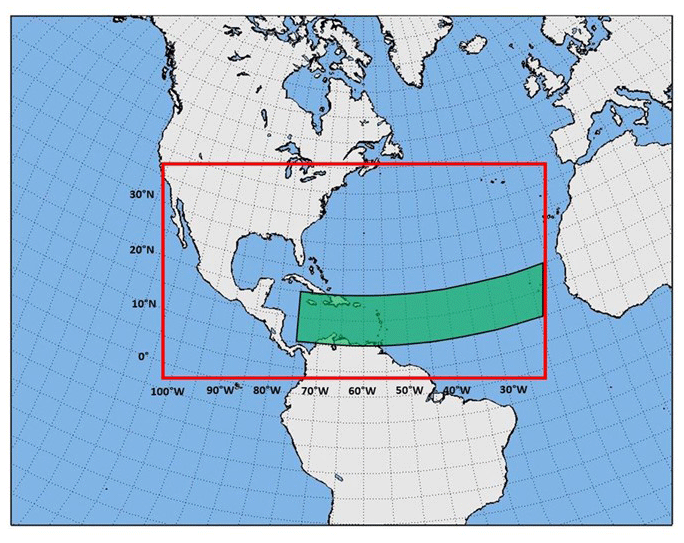
Figure 1 CRCM6 simulation domain (red box). The black/green shaded box shows the approximate present-day tropical cyclone main development region (MDR). Note that the data are projected over an equidistant cylindrical projection.

2.2 Experimental design

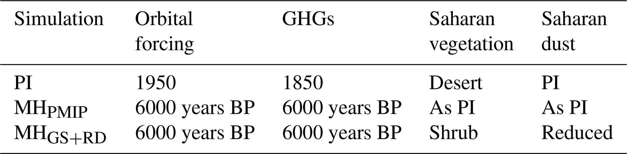
We performed three distinct 30-year experiments with CRCM6 (see Table 1). The first experiment, the control or reference case, is a pre-industrial (PI; performed at 0.11 and 0.22^∘ for validation purposes only) climate simulation that follows the protocol set by the Paleoclimate Modelling Intercomparison Project (PMIP) and the fifth phase of the Coupled Model Intercomparison Project (CMIP5) (Taylor et al., 2012). Two MH simulations were also performed: in the first one, the PMIP protocol is followed, only accounting for changes in the orbital forcing (∼5 % increase in Northern Hemisphere insolation compared to present-day values) and the greenhouse gas concentrations (MH_PMIP) relative to PI. The aim here is to evaluate the effect of the insolation forcing alone on TC activity compared to the reference case. In the second MH experiment, in addition to the changes in the MH_PMIP, the Sahara (11–33^∘ N, 15^∘ W–35^∘ E) was replaced by evergreen shrub and airborne dust concentrations reduced by up to 80 % in the EC-Earth experiment (MH_GS+RD) relative to PI. Due to those changes in vegetation in the Sahara, the albedo of the region decreased from 0.30 to 0.15 and the leaf area index increased from 0.2 to 2.6 (for details refer to Pausata et al., 2016, and Gaetani et al., 2017). GEM has a basic representation of aerosol, accounting for only the extinction coefficient, single scattering albedo and asymmetry factor for continental and maritime particles. These values are spread evenly over the longitudes with higher values at the Equator and lower at the poles and higher values over land than over the ocean. Given such a coarse representation of the aerosol optical properties, we did not change them when performing the regional MH_GS+RD experiment. Therefore, the major impacts of dust changes in the regional simulation (MH_GS+RD) were accounted for through the changes in the prescribed SST and lateral boundary conditions.

Table 1 Boundary conditions for each modeling experiment.

2.3 Tracking algorithm

In this study, a storm-tracking algorithm was developed using a three-step procedure (storm identification, storm tracking and storm lifetime) to detect tropical cyclones, following previous studies (Gualdi et al., 2008; Scoccimarro et al., 2011; Walsh et al., 2007). In comparison to most routines, our algorithm performs a double filtering approach similar to that applied in Caron and Jones (2012) to ensure that the genesis and dissipation phases of TCs are well represented and that TCs are not counted twice in the case of a temporary decrease of intensity followed by a restrengthening. Looser detection criteria (with lower values than the standard thresholds values) were first used in order to detect all storm centers; then criteria were enforced to standard values following the literature (strict criteria). Centers that satisfy the strict criteria are then classified as being “strong” centers (storm identification), while the others are classified as “weak” centers. To correctly represent each track (storm tracking), the strong and weak centers are then paired following two different methods: the storm history using a similar approach to that of Sinclair (1997) and the nearest-neighbor method as in Blender et al. (1997), Blender and Schubert (2000) and Schubert et al. (1998). Once the storm tracks are defined, the algorithm determines the core of each track as the centers sitting between the first and the last strong centers found in the track, thus neglecting the genesis and dissipation phases. This subsection of the track (representing the main TC lifetime) has to satisfy a third set of criteria that reject TCs that do not live long enough, that do not travel a long-enough distance or that do not reach the strength of a tropical storm. If the core of the storm track satisfies all these criteria, the genesis and dissipation phases (represented by the weak centers that occurred before the first and after the last strong centers) are added to form the complete storm track. A detailed description of the storm identification and tracking can be found in Appendix A.

2.4 Potential intensity and genesis indices

Many environmental proxies have been used to link the changes in the dynamical and thermodynamical fields to TC activity. Here, two well-known environmental proxies were adopted – the potential intensity (V_PI) and the genesis potential index (GPI) – to investigate the changes between different climate states in TC achievable intensity and in the areas more prone to develop TCs, respectively. To calculate the theoretical maximum intensity of TCs given specific environmental conditions, the V_PI formulation includes the SST, the temperature at the level of convective outflow (T_o), the ratio of drag and enthalpy exchange coefficients ($C_k/C_{\mathrm{d}}=\mathrm{0.9}$) and the available potential convective energy difference between an air parcel lifted from saturation at sea level (CAPE^*) at the radius of maximum winds and an air parcel located in the boundary layer (CAPE_b). The formula defined by Emanuel (1995) and updated by Bister and Emanuel (1998, 2002) was used to account for dissipative heating:

$$\begin{array}{}\text{(1)}& V_{\mathrm{PI}}=\sqrt{{\displaystyle \frac{C_k\cdot \text{SST}}{C_{\mathrm{d}}\cdot T_{\mathrm{o}}}}\left({\text{CAPE}}^{*}-{\text{CAPE}}_{\mathrm{b}}\right)}.\end{array}$$

The GPI is an empirical fit of the most important environmental variables known to affect TC formation. These variables include dynamical (wind shear and absolute vorticity) and thermodynamical (potential intensity and moist entropy deficit) factors. The first genesis index was introduced by Gray (1975, 1979). Since then, various genesis indices have been formulated (e.g., Emanuel and Nolan, 2004; Emanuel, 2010; Korty et al., 2012). Here, the genesis index formulation from Korty et al. (2012) was used, which is a modified version of the GPI described in Emanuel (2010). This GPI includes the entropy deficit between different atmospheric levels, as the one of Emanuel (2010), with the addition of the “clipped vorticity” (Tippett et al., 2011):

$$\begin{array}{}\text{(2)}& \text{GPI}={\displaystyle \frac{a{\left[min\left(\left|\mathit{\eta }\right|,\mathrm{4}\times {\mathrm{10}}^{-\mathrm{5}}\right)\right]}^{\mathrm{3}}{\left[max\left(V_{\mathrm{PI}}-\mathrm{35},\mathrm{0}\right)\right]}^{\mathrm{2}}}{{\mathit{\chi }}^{\mathrm{4}/\mathrm{3}}{\left[\mathrm{25}+V_{\mathrm{shear}}\right]}^{\mathrm{4}}}},\end{array}$$

where V_PI is the potential intensity, V_shear is the wind shear between 250 and 850 hPa levels, η is the absolute vorticity at 850 hPa, and a is a normalization coefficient. The entropy deficit χ is defined as

$$\begin{array}{}\text{(3)}& \mathit{\chi }={\displaystyle \frac{s_{\mathrm{b}}-s_{\mathrm{m}}}{s_{\mathrm{o}}^{*}-s_{\mathrm{b}}}},\end{array}$$

where s_b, s_m and $s_{\mathrm{o}}^{*}$ represent, respectively, the moist entropies of the boundary layer (900 hPa), middle troposphere (600 hPa) and the saturation entropy at the sea surface. Other indices have shown similar performance to the GPI, as, for example, the tropical cyclone genesis index (TCGI; Tippett et al., 2011; Menkes et al., 2011).

2.5 Regional model evaluation

To evaluate the CRCM6 performance in simulating tropical cyclones, an additional 0.22^∘ simulation was carried out using the ERA-Interim reanalysis as lateral boundary conditions and SSTs, and compared with 25 km ERA5 reanalysis data for the period 1980 to 2009 (see Hersbach et al., 2018). Our storm-tracking algorithm was used to detect tropical cyclones in the ERA5 reanalysis for validation and to ensure the accuracy of simulated results against the observed track density obtained from the Atlantic “best-track” dataset (the revised Atlantic hurricane database; HURDAT2) (Landsea and Franklin, 2013) for the same period (1980–2009). The use of the high-resolution ERA5 reanalysis data allowed us to directly compare the obtained results to our modeled 0.22^∘ data and the HURDAT2 observations. The comparison between the detected TCs in ERA5 reanalysis data and the observed TCs from the HURDAT2 database also provided a quick test case to evaluate ERA5 ability to represent observed TCs while using the same detection criteria, which cannot be done with the coarser resolution of the raw ERA-Interim data (∼80 km). The model evaluation is presented in Appendix A. In general, our tracking algorithm captures well the main characteristics of the observed tracks (Fig. A1). However, the number of detected TCs in ERA5 data is lower than observations, even when considering lower threshold values. On the other hand, when comparing the ERA-Interim-driven model-simulated TCs in the simulation against observations, there is a better agreement in the mean track characteristics and number of Atlantic TCs (Fig. A1a). Murakami (2014) and Hodges et al. (2017) found significant biases in the representation of TCs in various reanalysis datasets, using different tracking algorithms. Although these results strongly stem from the tracking algorithm's ability to capture weaker storms, our comparison between the HURDAT2 TC tracks and those obtained with ERA5 reanalysis shows important differences between the two.

In this study, we use a two-tailed Student t test to determine the statistical significance of changes at the 5 % confidence level. The significance of the changes in TC frequency has been determined using twice the standard error of the mean (∼5 % confidence level). The accumulated cyclone energy (ACE; Bell et al., 2000) was also calculated. ACE is defined as the sum of the square of the maximum sustained wind speed (in knots; 1 kn =0.514 m s⁻¹) higher than 35 kn every 6 h over all the storm tracks. ACE is an integrated measure depending on TC number, intensity and duration, and less sensitive than TC counts to tracking schemes and thresholds (Zarzycki and Ullrich, 2017). Besides the total ACE, the mean ACE per storm was also considered, and ACE per mean storm duration, in order to analyze the contribution of the different components of ACE to the total value.

To evaluate the statistical significance in the difference in TC counts between different climate states, a bootstrap method was used to create 100 randomly selected 30-year samples out of the 40-year (1979–2018) distributions of the annual number of observed TCs and ERA5 TCs.

3 Results

In this section, the TCs in the MH and PI climate conditions are studied to evaluate how changes in orbital forcing, dust and vegetation feedbacks impact TC activity in the Atlantic Ocean, by focusing on TC trajectories and annual frequency (Sect. 3.1), seasonality (Sect. 3.2) and intensity (Sect. 3.3). We also highlight the impacts of such changes on the different variables known to affect TC genesis.

3.1 Change in TC density and frequency

The PI climate simulation has a spatial distribution of Atlantic hurricanes that is similar to present climate, where most of the TCs form in the main development region (MDR) and move west–northwestward towards the North American east coast (Fig. 2b). However, there are fewer TCs in the simulated PI climate than in the present-day climate simulation driven by ERA-Interim (cf. Fig. 2a and A2); this is due to a large extent to the SST cold bias in the EC-Earth simulation (∼5 ^∘C; see Fig. A3). When only the orbital forcing is considered (MH_PMIP), there is a northward shift of the Atlantic TC tracks, as well as an eastward displacement of the tracks away from the US east coast at higher latitudes and a small increase in the TC track density relative to the PI experiment (Fig. 2c). This anomaly pattern is similar to that of the MH_GS+RD experiment, but the anomalies are notably stronger in the latter simulation (Fig. 2d), extending further north and westward into the Greater Antilles and Gulf of Mexico. The TC northward shift in the MH experiments and the strong eastward shift at higher latitudes are related to both the northward displacement of the ITCZ and the intensification of the WAM relative to the PI simulation (Fig. A4).

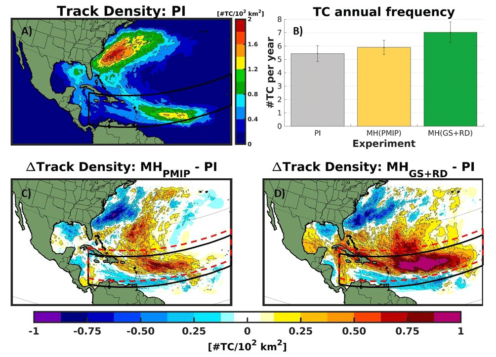
Figure 2 June to November (JJASON) climatology of (a) track density for the pre-industrial (PI) experiment; (b) TC frequency in the Atlantic Ocean for each experiment. Error bars (whiskers) indicate the standard error of the mean; changes in track density for the MH_PMIP (c) and the MH_GS+RD (d) experiments relative to the PI. The black box shows the present-day MDR; the dotted red box shows the approximate shift of the MDR in the MH experiments. Only values that are significantly different at the 5 % level using a local (grid-point) t test are shaded. The contour lines follow the color-bar scale (dashed, negative anomalies; solid, positive anomalies); the 0 line is omitted for clarity.

The northward shift of the ITCZ in the MH is due to energetic constraints associated with the changes in orbital forcing causing a warming of the NH and a cooling of SH during boreal summer relative to PI (Merlis et al., 2013; Schneider et al., 2014; Seth et al., 2019). The ITCZ is associated with more favorable conditions for cyclogenesis by increasing the ambient vorticity and therefore the TC activity (Merlis et al., 2013). Our analysis shows that the absolute vorticity maximum undergoes a northward shift relative to the control experiment, following the ITCZ displacement (Fig. A5), supporting the northward shift of the TC tracks (Fig. 2c). Higher absolute vorticity values are also found over the Greater Antilles and the western part of the Gulf of Mexico where there is a higher TC occurrence in the MH_GS+RD relative to PI.

The northward shift and the increase of TC activity in the MH experiments are also related to the strengthening of the WAM, which amplifies the westerly winds, and the SST anomaly (Fig. A6). Such changes lead to the development of a wind shear pattern anomaly in the MDR, with lower values of wind shear in the central–western region of the MDR and higher values on the eastern side of the MDR relative to PI. Thus, while the area more favorable for TC development is reduced (Fig. A7), the more favorable conditions present on the western side more than compensate the decrease in the east, allowing more cyclones to develop in the MH experiment. In addition to the zonal atmospheric circulation changes, the enhanced northward penetration of the WAM together with the displacement of the ITCZ leads to a northward shift of the maximum in AEW activity in the MH experiments relative to PI (see Fig. A8). The poleward displacement of the AEWs may also contribute to the changes in TC genesis location as they influence the region where TCs develop (e.g., Caron and Jones, 2012).

The vegetation changes and the associated reduction in dust concentrations further strengthen the WAM in the MH_GS+RD relative to the MH_PMIP experiment (Pausata et al., 2016, 2017), hence amplifying the changes seen in the MH_PMIP. Furthermore, the reduction in dust concentration in the MH_GS+RD experiment directly affects the SST (Fig. A6b), leading to an environment more prone to develop TCs relative to the MH_PMIP and PI simulations. This is consistent with previous studies that found that the Saharan dust layer can have large impacts on TC activity (Evan et al., 2016; Pausata et al., 2017; Reed et al., 2019).

The GPI anomalies of both MH experiments relative to PI closely follow the changes in the atmospheric and oceanic environmental factors that can affect TCs (cf. Figs. 3, A5–A9). The GPI shows more favorable conditions with higher values of vorticity and SST and lower wind shear values. Similarly to the absolute vorticity field (Fig. A5), the GPI shows a small northward shift relative to the control experiment, thus contributing to the poleward displacement of the TC genesis locations and therefore the the TC tracks (cf. Figs. 3 and 4).

Figure 3 Changes in seasonal GPI (JJASON) for (a) MH_PMIP and (b) MH_GS+RD experiments relative to PI. The black box shows the approximate present-day MDR. Only values that are significantly different at the 5 % level using a local (grid-point) t test are shaded. The contour lines follow the color-bar scale (dashed, negative anomalies; solid, positive anomalies); the 0 line is omitted for clarity.

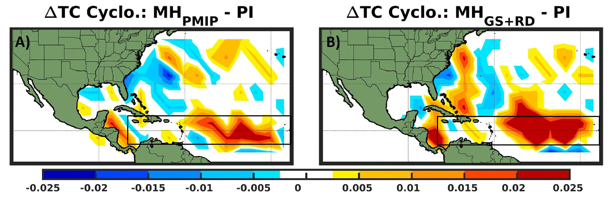
Figure 4 TC seasonal (JJASON) cyclogenesis density anomaly for (a) MH_PMIP and (b) MH_GS+RD experiments relative to PI represented over a 5^∘ mesh-grid Mercator projection. The black box shows the approximate present-day MDR.

The largest changes in GPI are seen in the MH_GS+RD experiment (Fig. 3b). The greening of the Sahara and the reduced dust concentrations over the Atlantic Ocean not only lead to higher potential for cyclogenesis in the MDR but also extend the region westward towards the Caribbean where the model simulates a higher occurrence of TCs in this experiment relative to the PI (see Fig. 2c). Overall, the changes in cyclogenesis density for both MH experiment follow closely the changes in GPI (cf. Figs. 3 and 4), suggesting that GPI is a good predictor of the TC activity changes, even in very different climate states. Moreover, in Pausata et al. (2017), the TC genesis anomalies in the MH experiments show a westward shift, while in our analysis the TC genesis anomalies relative to PI present a net northward displacement of its locations, highlighting an important difference between the two downscaling techniques (see Fig. A10). These changes in the TC genesis are likely responsible for the downstream changes in the TCs' track density in both studies.

In terms of frequency, an average of 5.5 TCs per year is simulated in the PI experiment (Fig. 2b). This is ∼45 % less than the present-day climatology (∼10 TCs per year; Landsea, 2014), which is likely due to a strong cold bias in the SST of the coupled model simulation (see Fig. A3 and Pausata et al., 2017). Many high-resolution global models have similar biases in the Atlantic (e.g., Shaevitz et al., 2014; Wing et al., 2019). The MH_PMIP experiment shows a small increase (+9 %; statistically significant) in the TC frequency relative to the PI, highlighting the minor impact of the orbital forcing alone on the number of Atlantic TCs (Fig. 2b). In the MH_GS+RD simulation, more TCs are generated (7 per year) with a significant increase of around 1.5 TCs per year (+27 %) relative to the PI experiment (Fig. 2b). Bootstrap tests with both HURDAT2 (Fig. 5a) and ERA5 (Fig. 5b) datasets show that the chances of obtaining an increase of 27 % (9 %) in the mean of each distribution are significantly (slightly) higher than the 95th percentile of these distributions. Our sensitivity experiments hence roughly show that the orbital forcing alone contributes for about 33 % (∼0.5 TCs per year) of the total increase in TC frequency occurring in the MH_GS+RD relative to the PI experiment, while the Saharan greening and reduced dust concentrations account for about 66 % of this increase (∼1 TC per year). Thus, these results suggest that the TC activity is strongly dominated by the vegetation and dust changes, in close agreement with Pausata et al. (2017).

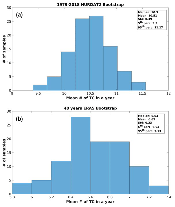
Figure 5 Bootstrap distributions based on (a) the 1979–2018 HURDAT database and (b) 1979–2018 ERA5 reanalysis data. The legend presents the median, mean, standard deviation, 5th and 95th percentiles of the distributions.

3.2 Changes in TC seasonal cycle

To analyze changes in TC seasonal cycle, we consider changes in the monthly number of TCs rather than change of the length of the TC season. The PI climate has a TC seasonal cycle that is similar to the present climate, with a peak in TC in September (Fig. 6). The MH experiments show a distinct pattern: a decrease in TC activity at the beginning of the hurricane season for both MH experiments (statistically significant for the MH_PMIP in July and August; non-significant for the MH_GS+RD), followed by a large increase at the end of TC season (statistically significant during September and October in the MH_PMIP; MH_GS+RD from September to November, SON) relative to PI.

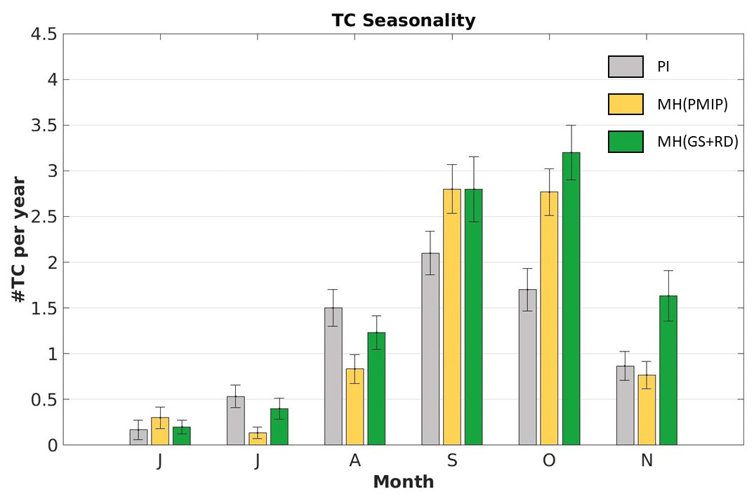
Figure 6 TC climatological distribution throughout the extended TC season (JJASON) for each experiment. Error bars (whiskers) indicate the standard error of the mean.

Gaetani et al. (2017), using the same global model experiments performed with EC-Earth, showed a large decrease in the AEWs in the MH_GS+RD relative to the MH_PMIP simulation due to the strengthening of the WAM. As AEWs can potentially act as seeds for TC genesis (Caron and Jones, 2012; Frank and Roundy, 2006; Landsea, 1993; Thorncroft and Hodges, 2001), we analyze the changes in the AEW seasonality in the MH experiments relative to PI to determine whether there is a direct link between the changes in the seasonality of AEW and TCs (Fig. 7). The AEWs' activity is remarkably reduced between July and September – 80 % less relative to PI – and intensified in October and November in the MH_GS+RD relative to PI (Fig. 7b).

Figure 7 Monthly AEW anomalies represented through the variance of the meridional wind at 700 hPa, filtered in the 2.5 to 5 d band, for (a) MH_PMIP and (b) MH_GS+RD relative to PI. The black box shows the approximate present-day MDR. Only values that are significantly different at the 5 % level using a local (grid-point) t test are shaded. The contour lines follow the color-bar scale (dashed, negative anomalies; solid, positive anomalies); the 0 line is omitted for clarity.

The reduction of the AEWs in the MH_GS+RD experiment is related to the strengthening and northward shift of the WAM. The anomalous westerly wind flow associated with the northward expansion of the WAM rainfall significantly alters the African easterly jet (AEJ) (Fig. 8) and the Saharan heat low. In particular, the disappearance of the 600 hPa AEJ and northward displacement of the wind circulation are responsible for the lower frequency of AEWs during the summer months in the MH_GS+RD relative to PI. On the other hand, the withdrawal phase of the WAM towards the end of the season (SON) is associated with an increase in the frequency of AEWs relative to PI, potentially contributing to the increase in TC activity in those months. While the changes in the frequency of AEWs in the MH_GS+RD are potentially in agreement with the simulated changes in TC seasonality, the frequency of AEWs in the MH_PMIP is higher relative to PI, especially in June and July, which is at odds with the changes in TC frequency in the MH_PMIP experiment (no change in June and slight decrease in July; Fig. 7a). Furthermore, in July and August, fewer TCs are simulated in the MH_PMIP relative to the MH_GS+RD, which has fewer AEWs. Hence, it is not possible to draw a direct link between the changes in the seasonality of AEWs and TCs between the MH and the PI simulations. These results agree with the findings of Patricola et al. (2018) that, while AEWs can affect TC genesis, their contribution may not be necessary, and TCs can also be formed from other processes such as wave breaking of the ITCZ, disturbance from the Asian monsoon trough or self-aggregation of convection (Patricola et al., 2018). Furthermore, Vecchi et al. (2019) showed that a combination of the large-scale environmental factors (in particular ventilation) and the frequency of disturbances determined the TC frequency in their model.

Figure 8 AEJ represented through a vertical cross section of zonal mean (0–40^∘ N; 20–30^∘ W) seasonal climatological zonal winds for (a) PI and (b) MH_GS+RD experiments, respectively.

Other factors could be playing a role in modifying the TC seasonal cycle. In particular, the shift in TC seasonal cycle could be related to changes in the orbital forcing, most importantly the precession of the equinoxes: during the MH, the perihelion was in September instead of January, as today, with the stronger insolation anomalies peaking in late summer at NH low latitudes. Furthermore, while higher potential intensity (due mostly to warmer SSTs; see Figs. A6 and A11) develops on the western part of the MDR and most of the North Atlantic Ocean from June to September relative to the PI experiment, the strengthening of the WAM causes a cold anomaly response over the eastern part of the MDR, together with stronger vertical wind shear and weaker absolute vorticity values. The withdrawal of the WAM in late September then causes the decrease in wind shear and positive anomalies in both absolute vorticity and SSTs to extend eastward. These environmental anomalies are likely the reason for the TC seasonality changes during the MH experiments (Figs. A11a, A12a, A13a). The cyclogenesis anomalies and the GPI changes are consistent with these assumptions (cf. Figs. 9a and A14a). Korty et al. (2012), who studied the response to orbital forcing in PMIP2 models during the MH, also found that the TC season in the Northern Hemisphere was less favorable during summer, while it became more favorable during fall (October and November) relative to pre-industrial climate. The authors pointed out that these findings were due to the difference between the warming rate of the atmosphere (which warms faster during the summer months) and that of the ocean surface, which led to a negative potential intensity anomaly during the first half of their TC season (June to September) and a positive anomaly during the second half (October to November). Using PMIP3 models, Koh and Brierley (2015) drew similar conclusions; however, the changes in fall were not a robust signal across models.

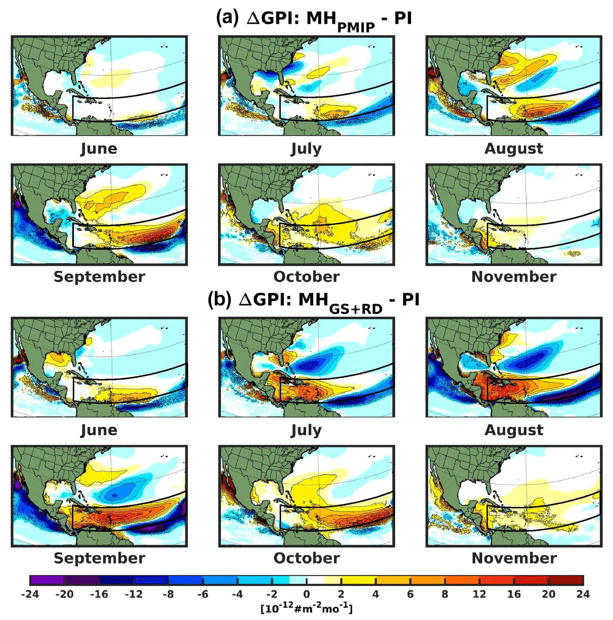
Figure 9 Changes in climatological monthly GPI for (a) MH_PMIP and (b) MH_GS+RD relative to the PI experiment. The black box shows the approximate present-day MDR. Only values that are significantly different at the 5 % level using a local (grid-point) t test are shaded. The contour lines follow the color-bar scale (dashed, negative anomalies; solid, positive anomalies); the 0 line is omitted for clarity.

Accounting for the Saharan greening and reduced airborne dust concentrations (MH_GS+RD) leads to even larger changes relative to PI (Figs. A11b, A12b, A13b), strengthening the GPI anomalies in the MDR (Fig. 9b). These changes strongly increased the total GPI over the ocean from September to November in the MH_GS+RD experiment and led to almost twice as many cyclones in November relative to the PI and MH_PMIP experiments (see Figs. 6, 10 and A14b). Furthermore, there is a westward extension of the region prone to TC development towards the Greater Antilles and the Caribbean Sea from July to September relative to the other two experiments (Figs. 9b and 11), which is also reflected in the seasonal GPI (Fig. 3b). These anomalies led to a small increase in cyclogenesis over the Caribbean Sea relative to PI during this part of the season and may explain the increased TC activity during July and August in the MH_GS+RD relative to the MH_PMIP and why almost as many cyclones formed during September (cf. Figs. 6, A14).

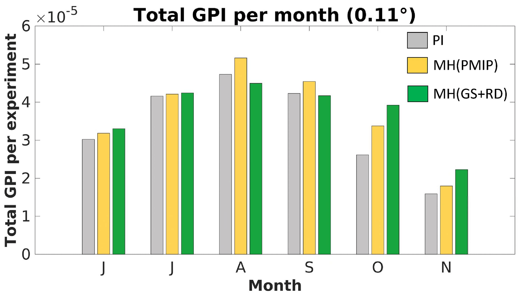
Figure 10 Seasonal variation (JJASON) of the GPI summed over the experimental domain for the three experiments.

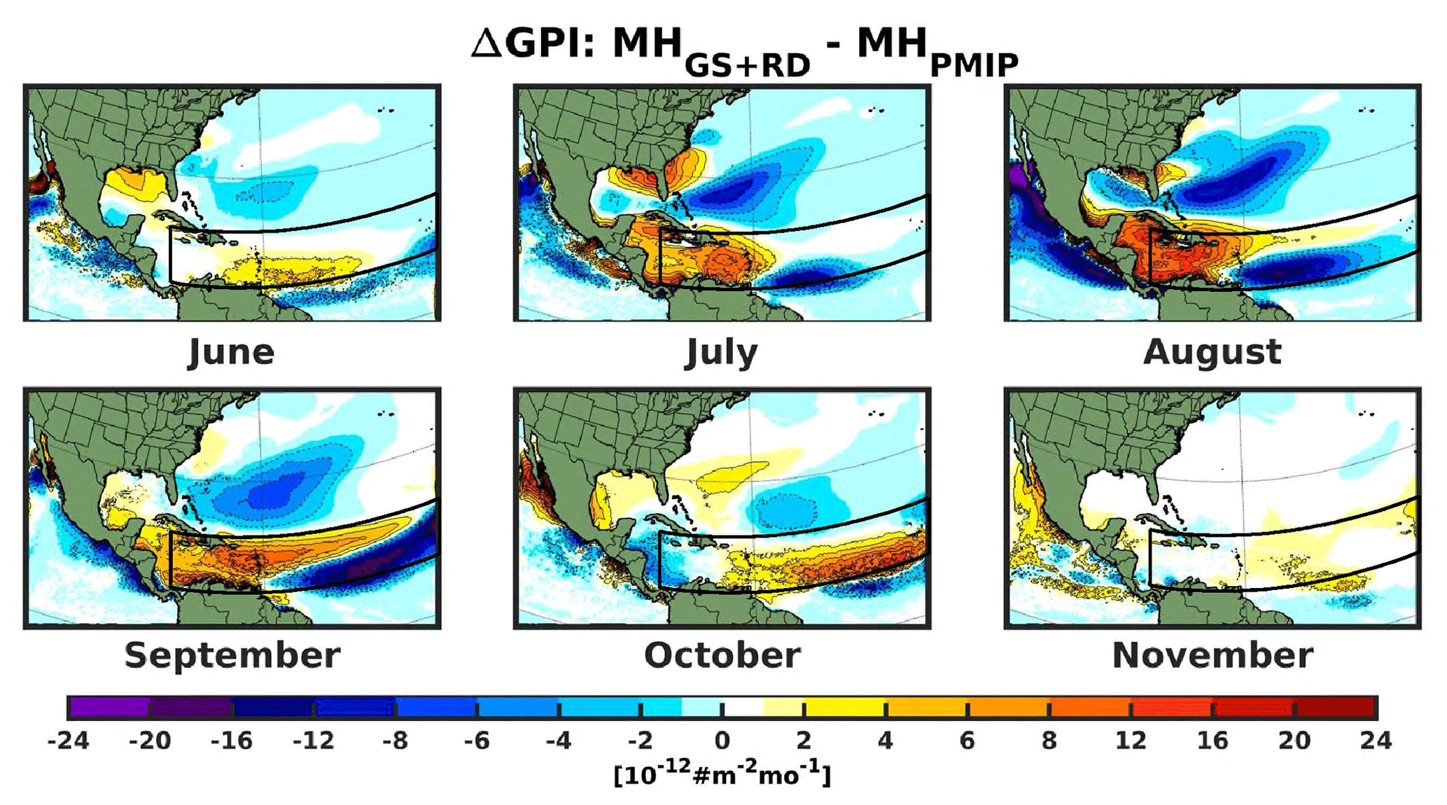
Figure 11 Changes in climatological monthly GPI for MH_GS+RD relative to the MH_PMIP experiment. The black box shows the approximate present-day MDR. Only values that are significantly different at the 5 % level using a local (grid-point) t test are shaded. The contour lines follow the color-bar scale with different styles (dashed, negative anomalies; solid, positive anomalies); the 0 line is omitted for clarity.

3.3 Changes in intensity

To assess TC intensity, we considered the 10 m maximum wind speed in 3 h intervals and then classified them using the Saffir–Simpson scale categories. For the three experiments, most tropical cyclones reach only tropical storm or hurricane Category 1 (93 %, 88 % and 91 % for PI, MH_PMIP and MH_GS+RD, respectively), with only a few reaching Category 2 (7 %, 11 % and 8 %) (Fig. 12). Both MH simulations generated Category 3 hurricanes (∼1 % in both cases), while there were no major hurricanes in the PI experiment. Our analysis of the ACE also reveals that, in general, the mean ACE per cyclone in the MH experiments is higher than in the PI experiment ($\sim \mathrm{6.6}\times {\mathrm{10}}^{\mathrm{4}}$ m² s⁻² and $\sim \mathrm{7.4}\times {\mathrm{10}}^{\mathrm{4}}$ m² s⁻² for MH_PMIP and MH_GS+RD, respectively, $\sim \mathrm{6.1}\times {\mathrm{10}}^{\mathrm{4}}$ m² s⁻² for PI; see legend in Fig. 13c). The increase in ACE in MH simulations arises from two different aspects: (1) TCs in the MH climate are more intense than in the PI experiment (as shown in Fig. 12), therefore leading to higher rate of energy generation, and (2) TCs in the MH experiments tend to last longer (PI: 199 h, MH_PMIP: 217 h and MH_GS+RD: 283 h; see legend in Fig. 13c), meaning that the same amount of energy can be spend over a longer time lapse. The combination of these two aspects with increased mean TC count per season in the MH experiments (Figs. 2b and 14a) therefore leads to a larger total mean ACE per experiment in the MH simulations compared to PI (see legend in Fig. 13b).

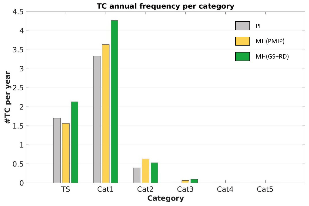
Figure 12 Climatological number of TCs per year in various categories for the three experiment during the TC extended season (JJASON).

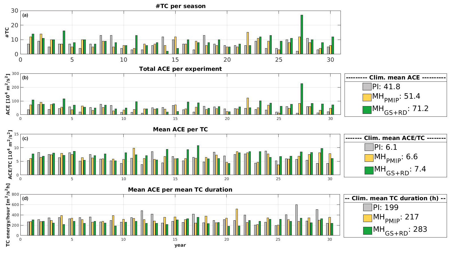
Figure 13 (a) Total number of cyclones per season for each experiment (30 years; gray: PI, yellow: MH_PMIP and green: MH_GS+RD). (b) Total ACE (10⁴ m² s⁻²). (c) Mean ACE per cyclone per season (10⁴ m² s⁻²). (d) Mean ACE per cyclone normalized by the mean tropical cyclone duration in every season (10⁴ m² s⁻² h⁻¹). Legends present the climatological mean of each distribution.

To better understand the cause of these changes, we turn to the seasonal V_PI (Fig. 14) and examine the regions where the atmospheric conditions are more favorable for TC intensification. The area showing the most favorable conditions for cyclone intensification in the MH_PMIP relative to the PI experiment is located around the central–western portion of MDR and extends northwards over the central Atlantic Ocean and westward along the northernmost part of the US east coast (Fig. 14a). Less favorable conditions are present east and south of the MDR where colder SSTs are present. The mean V_PI pattern for the MH_GS+RD yields even stronger anomalies than the ones simulated by the MH_PMIP, with substantially more favorable conditions for intensification in the MDR (Fig. 14b). More conducive conditions are also present in the Caribbean Sea, where markedly lower values of vertical wind shear are simulated (Fig. A7). The combination of more favorable environmental conditions (e.g., wind shear) along with the occurrence of more TCs crossing this area in the MH_GS+RD experiment relative to both PI and MH_PMIP (see Fig. 2d) increases the chances of getting more intense and long-living cyclones. The main factors contributing to the increase in V_PI in the MH_GS+RD relative to the PI and MH_PMIP experiments are the warmer SSTs (∼1.5 ^∘C higher; Fig. A6b) and enhanced levels of convective available potential energy (CAPE; Fig. A15) as direct consequences of the reduced dust emissions. In comparison to the change seen in the MH_PMIP relative to PI, less favorable conditions for intensification are simulated north of the MDR in the MH_GS+RD (Fig. 14b). Overall, the V_PI anomalies for both MH experiments strongly resemble those presented in Pausata et al. (2017) and closely follow the changes in GPI, therefore leading to more intense and potentially longer-living cyclones where better conditions are available for cyclogenesis.

Figure 14 Changes in climatological seasonal V_PI (JJASON) for the (a) MH_PMIP and (b) MH_GS+RD experiments relative to PI. The black box shows the present-day MDR. Only values that are significantly different at the 5 % level using a local (grid-point) t test are shaded. The contour lines follow the color-bar scale (dashed, negative anomalies; solid, positive anomalies); the 0 line is omitted for clarity.

4 Discussion and conclusions

In this study, we use the CRCM6 regional climate model with a high horizontal resolution (0.11^∘) to better investigate the role played by vegetation cover in the Sahara and airborne dust on TC activity in the Atlantic Ocean during a warm climate period, the mid-Holocene (MH, 6000 years BP). We compared two different MH experiments – where only orbital forcing is considered (MH_PMIP) and where also changes in vegetation and dust concentration are accounted for (MH_GS+RD) – to a control PI experiment. Our results show that the Saharan greening and related reduction in dust concentrations (MH_GS+RD experiment) significantly increase the number of TCs in the North Atlantic Ocean by about 27 %, whereas the increase associated with the orbital forcing alone is smaller (9 %; MH_PMIP). In general, our results are consistent with the findings of Pausata et al. (2017), who used the same coupled global model simulation to drive a statistical–thermodynamical downscaling technique (Emanuel et al., 2008) to assess changes in TC activity; however, the changes in TC activity simulated in our study between the MH experiments and the PI simulation are smaller. Furthermore, the displacement of TC activity is different in our study (meridional vs. zonal) and most likely related to the fact that dynamical changes in ITCZ and AEW are not accounted for in Pausata et al. (2017). Our experiments show that the MH climate induces a northward shift of the North Atlantic TC tracks and an eastward displacement of those away from the US east coast at higher latitudes. A zonal shift of the storm track relative to PI is instead simulated in Pausata et al. (2017). Our work also suggests an important reduction of the TC activity during the first half of the TC seasonal cycle in the MH experiments together with a shift of the maximum TC activity towards the second half.

Gaetani et al. (2017) showed a strong decrease in AEW in the MH_GS+RD simulations and suggested a potential impact on TC activity; however, our analysis does not show a consistent relationship between the frequency of AEWs and tropical cyclones. These results support the findings of Patricola et al. (2018), who showed through a set of sensitivity experiments that the AEWs may not be necessary for TC genesis as TC formation occurs even in the absence of AEWs through other mechanisms. This is supported by observational studies that could not find a direct relation in the frequency of AEWs and TCs (Russell et al., 2017). Instead, the AEWs seem to play a more important role in the location of TC genesis rather than the total TC frequency. Furthermore, the RCM domain size and location of the lateral boundary conditions impact the frequency of AEWs TCs inside the domain (Caron and Jones, 2012; Landman et al., 2005).

Our study suggests that the different orbital parameters together with the changes in the WAM intensity may have been the main causes of the changes in TC seasonality, offering better conditions for cyclogenesis towards the end of the hurricane season. WAM intensity affects the wind shear on the eastern side of the MDR. The WAM withdrawal towards the end of the summer extended the more favorable conditions from the central–western portion towards the eastern portion of the MDR, causing an increase in TC activity during the second half of the season in the MH simulations. These results are consistent with the findings of Korty et al. (2012), who also showed higher cyclogenesis potential towards the end of the PI hurricane season in their MH experiment, with likely increase in TC activity during October when the GPI is at its maximum. However, their results are based on the entire Northern Hemisphere, while here we only focus on the North Atlantic Ocean. In addition, our results compare well to those of Koh and Brierly (2015), who found less favorable environmental conditions for TC development during Northern Hemisphere summer in the MH relative to pre-industrial when analyzing PMIP3 model simulations. Hence, the impact on TCs on changes in orbital forcing is consistent across different models and highlights an interesting point where there may be a repression of the modeled environmental conditions that negatively affects proxies associated with TC (i.e., the V_PI and GPI) and supports these results during the summer months, which is later offset by opposite changes during the autumnal season in many of them. Moreover, even if airborne dust variations are dominant in controlling the TC annual total, the orbital forcing still has a detectable role in affecting TC activity. Our work also shows that the GPI is able to represent the regions more prone to TC development in different climate states, in agreement with previous studies (Camargo et al., 2007; Koh and Brierley, 2015; Korty et al., 2012; Pausata et al., 2017). The reduced dust emissions in the MH_GS+RD experiment induce an additional SST warming that enhances the available thermodynamic energy, increasing the V_PI even further compared to the MH_PMIP and PI experiments and thus leading to more intense TCs. This SST warming-induced effect is consistent with the model-based projections for TC intensity in a warmer future climate (Knutson et al., 2013; Walsh et al., 2016; Knutson et al., 2020).

Finally, the simulated impact of dust changes needs further investigation, as rainfall in the north of Africa can be strongly affected by the dust optical properties (e.g., “heat pump” effect where the atmospheric dust layer warms the atmosphere, enhancing deep convection and intensifying the WAM; see Lau et al., 2009). In particular, in EC-Earth, dust particles are moderately to highly absorbing particles (single scattering albedo ω₀<0.95), with ω₀=0.89 at 550 nm. Such a value is too absorbing compared to observations (see Fig. 1 in Albani et al., 2014), and consequently the radiative impact of dust may well be overestimated. In a recent study, Albani and Mahowald (2019) showed how different choices in terms of dust optical properties and size distributions may yield opposite results in terms of rainfall changes. However, in the EC-Earth simulations, most of the changes in the WAM intensity were associated with changes in surface albedo due to greening of the Sahara, which was enhanced by dust reduction through a further decrease in planetary albedo. This response is opposite to what one would expect from a reduced heat pump effect (decreased rainfall), suggesting that the heat pump effect is overwhelmed by the changes in surface albedo under green Sahara conditions in EC-Earth simulations. Another important aspect that was not considered in our study is dust–cloud interactions which may further feed back in TC activity, both directly in the TC formation and indirectly by affecting the intensity of the WAM. A recent study (Thompson et al., 2019) showed that this interaction could indeed influence the WAM rainfall. Therefore, additional studies investigating the impact of dust optical properties and dust–cloud interactions on TC activity are needed.

In conclusion, our study highlights the importance of vegetation and dust changes in altering TC activity and calls for additional modeling efforts to better assess their role on climate. For example, employing regional model simulations with atmosphere and ocean coupling will be important to better represent the interactions between TC activity and TC–ocean feedbacks as a large amount of energy is transferred through TC activity between the atmosphere and the ocean (Scoccimarro et al., 2017). Furthermore, to validate the model results, additional new paleotempestology records across the Gulf of Mexico and Caribbean Sea will be of paramount importance. While our study shows an increase in TC frequency and intensity during a climate state with warmer summers and a stronger WAM, it is difficult to draw a direct conclusion for the future, as environmental proxies associated with TCs (i.e., the V_PI and GPI) are less sensitive to temperature anomalies caused by CO₂ than by those caused by orbital forcing (Emanuel and Sobel, 2013). However, in the view of a potential future “regreening” of the Sahel and/or reduced Saharan dust layer, as shown in Biasutti (2013), Evan et al. (2016) and Giannini and Kaplan (2019), our work suggests that these changes may further enhance TC frequency due to only greenhouse gases, in particularly over the MDR, the Greater Antilles and the western portion of the Gulf of Mexico, and could generate more intense and potentially longer-living cyclones, increasing the vulnerability of society to damages from severe TCs.

Appendix A: Tracking algorithm

In this study, we developed a tracking algorithm that makes use of a three-step procedure to detect cyclones, following previous studies (Gualdi et al., 2008; Scoccimarro et al., 2011; Walsh et al., 2007).

A1 Storm identification

The storms are identified with the following criteria:

• a.

  The surface pressure at the center must be lower than 1013 hPa and lower than its surrounding grid boxes within a radius of 24 km (2Δx); this pressure is then taken as the center of the storm.

• b.

  The center must be a closed pressure center so that the minimum pressure difference between the center and a circle of grid points in a small and a large radius around the center (200 and 400 km radii) must be greater than 1 and 2 hPa, respectively.

• c.

  There must be a maximum relative vorticity at 850 hPa around the center (200 km radius) higher than 10⁻⁵ s⁻¹.

• d.

  The maximum surface wind speed around the center (100 km radius) must be stronger than 8 m s⁻¹.

• e.

  To account for the warm core, temperature anomalies at 250, 500 and 700 hPa are calculated, where each anomaly is defined as the deviation from a spatial mean over a defined region. The sum of the temperature anomalies between the three levels must then be larger than 0.5 ^∘C.

• f.

  If there are two centers nearby, they must be at least 250 km apart from each other; otherwise, the stronger one is taken.

To identify the genesis and dissipative phases of the TCs, a double filtering approach was used, similar to that applied by Caron and Jones (2012). The aforementioned threshold values were used to first detect all the potential centers that could belong to a storm for each time step. Then, these criteria were enforced to the standard values (defined below) following the literature (Gualdi et al., 2008; Scoccimarro et al., 2011; Walsh, 1997; Walsh et al., 2007), and these new threshold values were applied to each center to identify the ones that satisfied these enforced criteria among the potential weak ones that were predefined. The centers that satisfied the standard criteria were labeled by the algorithm as being strong centers (or real TC centers), while those that only satisfied the first set of criteria were identified as being weak centers (with standard value properties defined below).

The enforced criteria are the following:

• a.

  surface pressure at the center deeper than 995 hPa;

• b.

  minimum pressure difference between the center and a 200 and 400 km radius greater than 4 and 6 hPa, respectively;

• c.

  relative vorticity maximum larger than 10⁻⁴ s⁻¹;

• d.

  wind speed maximum above 17 m s⁻¹; and

• e.

  warm core temperature anomaly above 2 ^∘C.

Another condition was added that only the strong centers needed to satisfy:

• f.

  The maximum wind velocity at 850 hPa must be larger than the maximum wind velocity at 300 hPa.

In doing so, we avoided double counting cyclones that may decreased in intensity before re-intensifying. Conditions (e) and (f) are the main conditions that filtered the TCs centers from other low-pressure systems and extratropical cyclones, as TCs have a warm core in their upper part and stronger low-level wind speed than other storms.

A2 Storm tracking

Storms were then tracked as follows: for each potential center found, the algorithm used the nearest-neighbor method, which was also applied in many other studies (Blender et al., 1997; Blender and Schubert, 2000; Schubert et al., 1998), to find a corresponding center in the following 3 h time interval within a 250 km radius around the storm center. Once two centers were paired, they formed a storm track. The potential position of the next center to be a continuation of the storm was then calculated using the storm history, based on the position of the previous two centers, which allowed us to establish a possible speed and direction for the predicted center. A similar procedure was applied in Sinclair (1997) and was derived from Murray and Simmonds (1991). The algorithm then searches around the last storm center using the nearest-neighbor method and around this potential position at the next time step to find a matching center. The nearest center was always chosen first.

A3 Storm lifetime

Once a track was completed, it had to satisfy the following final conditions:

1. The TC had to exist for at least 36 h (with a minimum of 12 centers at 3 h intervals).

2. The TC needed to have at least 12 strong centers along its entire track, so that the shortest TC had only strong centers (36 h).

3. The TC had to travel at least 10^∘ (∼1000 km) of combined longitude and latitude in its lifetime.

4. The number of strong storm centers needed to represent at least 77 % of a subpart of the complete storm track delimited by the first and last strong center found by the algorithm. This way, we ensured that the storm was classified as a TC during most of its time.

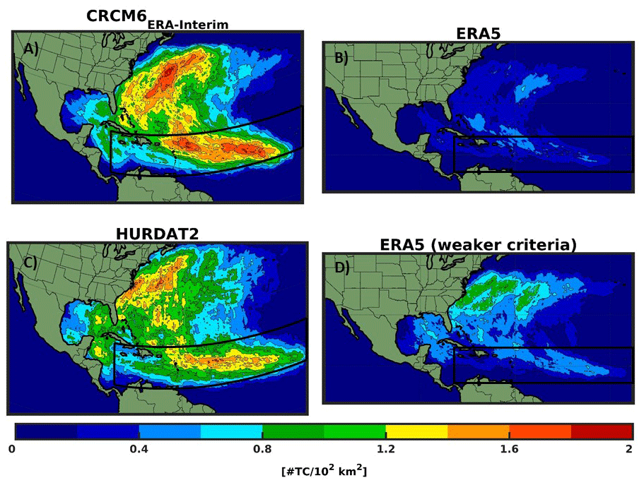
Figure A1 JJASON climatology (1980–2009) of (a) track density for the CRCM6 ERA-Interim-driven experiment at 0.22^∘; (b) ERA5 reanalysis data at 0.25 ^∘; (c) observed TCs from the HURDAT database at 0.11^∘ and (d) ERA5 reanalysis data using weaker detection criteria at 0.25^∘. The black box shows the present-day MDR. Note that the ERA5 figures are projected over a Mercator grid while the other two figures use the equidistant cylindrical projection. The contour lines follow the color-bar scale.

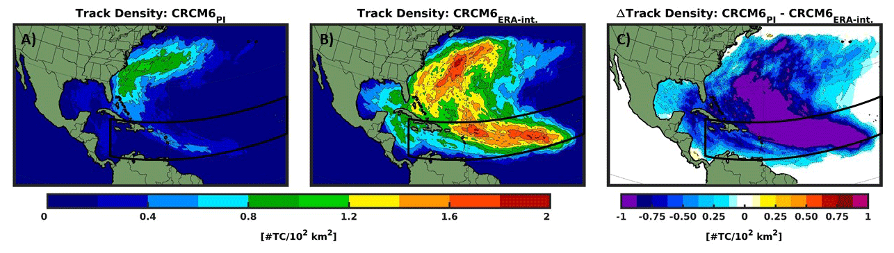
Figure A2 Climatological track density (JJASON) for the (a) pre-industrial experiment at 0.22^∘ and (b) ERA-Interim-driven experiment at 0.22^∘. (c) Changes in track density between the two simulations. The black box shows the approximate present-day MDR. Only values that are significantly different at the 5 % level using a local (grid-point) t test are shaded. The contour lines follow the color-bar scale (dashed, negative anomalies; solid, positive anomalies); the 0 line is omitted for clarity.

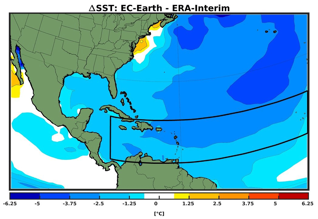
Figure A3 Climatological changes in SST between simulated EC-Earth pre-industrial climate and ERA-Interim reanalysis from 1979 to 2008. The black box shows the approximate present-day MDR. The contour lines follow the color-bar scale (dashed, negative anomalies; solid, positive anomalies); the 0 line is omitted for clarity.

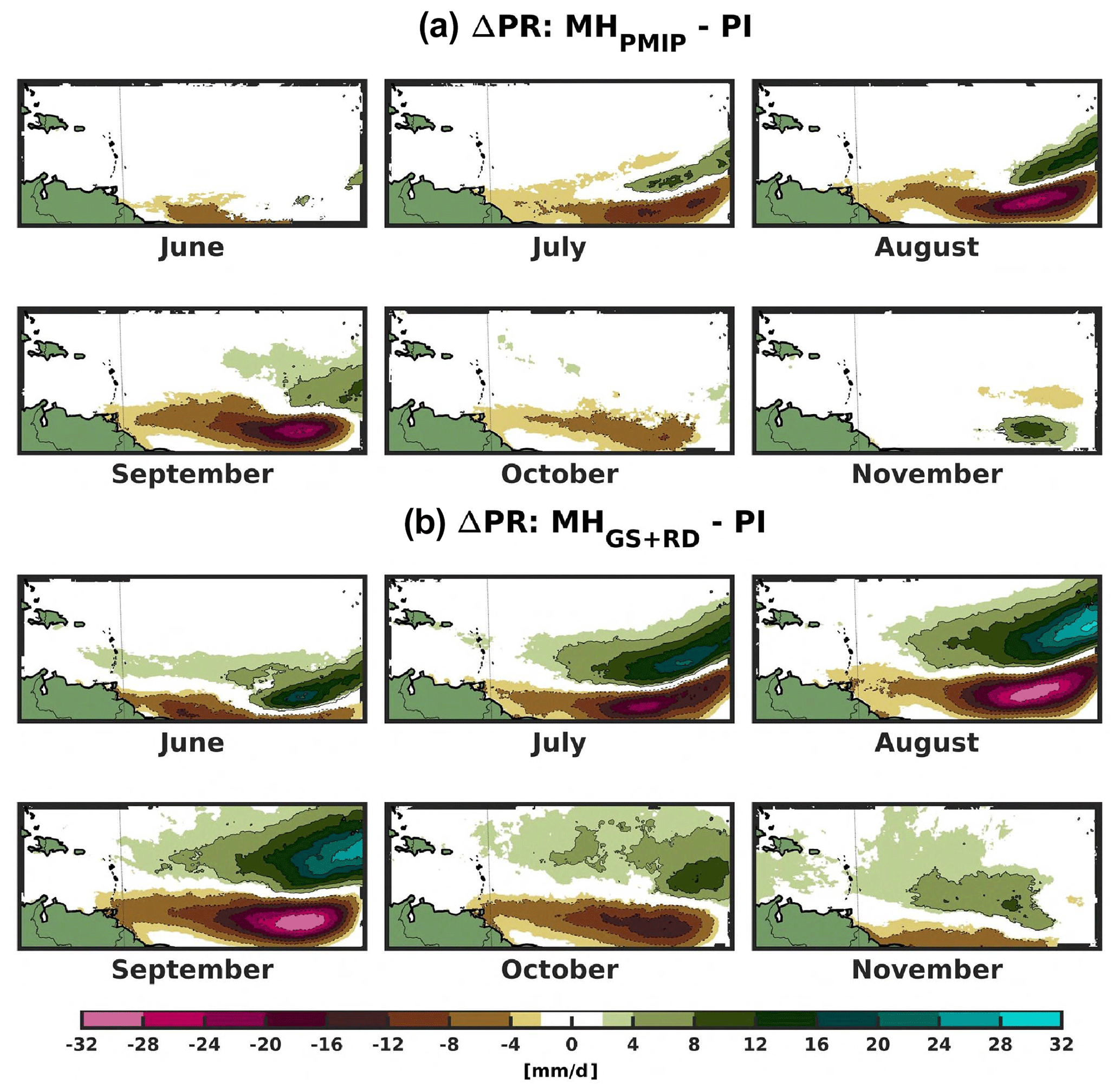
Figure A4 Monthly mean climatological changes in precipitation for (a) MH_PMIP and (b) MH_GS+RD relative to PI in the domain of 5–23^∘ N, 23–75^∘ W. Only values that are significantly different at the 5 % level using a local (grid-point) t test are shaded. The contour lines follow the color-bar scale (dashed, negative anomalies; solid, positive anomalies); the 0 line is omitted for clarity.

Figure A5 Climatological (JJASON) changes in 850 hPa absolute vorticity relative to PI for the (a) MH_PMIP experiment and (b) MH_GS+RD experiment. The black box represents the approximate present-day MDR. The dotted red box shows the approximate shift in the absolute vorticity maxima. Only values that are significantly different at the 5 % level using a local (grid-point) t test are shaded. The contour lines follow the color-bar scale (dashed, negative anomalies; solid, positive anomalies); the 0 line is omitted for clarity.

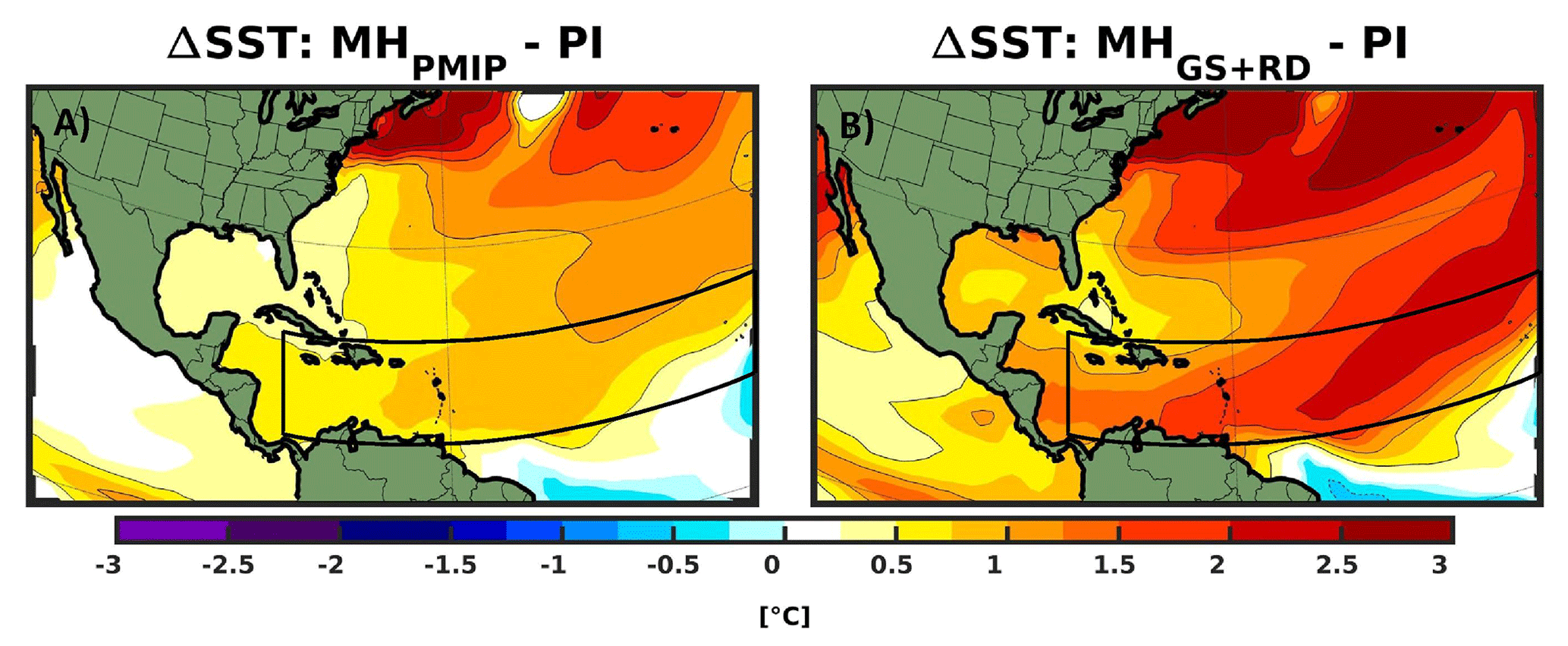
Figure A6 Climatological (JJASON) changes in SST for the (a) MH_PMIP and (b) MH_GS+RD experiments relative to PI. The black box shows the approximate present-day MDR. Only values that are significantly different at the 5 % level using a local (grid-point) t test are shaded. The contour lines follow the color-bar scale (dashed, negative anomalies; solid, positive anomalies); the 0 line is omitted for clarity.

Figure A7 Changes in vertical wind shear (300–850 hPa) for the (a) MH_PMIP and (b) MH_GS+RD experiments relative to PI. The black box shows the approximate present-day MDR. Only values that are significantly different at the 5 % level using a local (grid-point) t test are shaded. The contour lines follow the color-bar scale (dashed, negative anomalies; solid, positive anomalies); the 0 line is omitted for clarity.

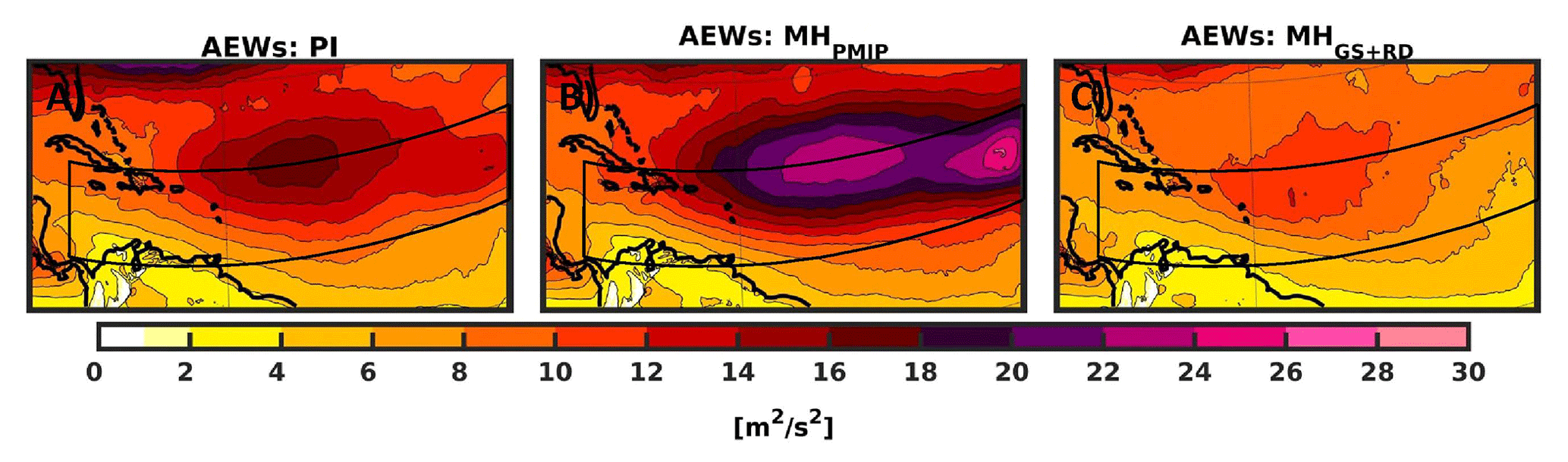
Figure A8 AEWs represented through the variance of the meridional wind at 700 hPa, filtered in the 2.5 to 5 d band, for the (a) PI, (b) MH_PMIP and (c) MH_GS+RD experiments. The black box shows the approximate present-day MDR. The contour lines follow the color-bar scale.

Figure A9 Climatological (JJASON) changes in 200 hPa wind speed for the (a) MH_PMIP and (b) MH_GS+RD experiments relative to PI. The black box shows the approximate present-day MDR. Only values that are significantly different at the 5 % level using a local (grid-point) t test are shaded. The contour lines follow the color-bar scale (dashed, negative anomalies; solid, positive anomalies); the 0 line is omitted for clarity.

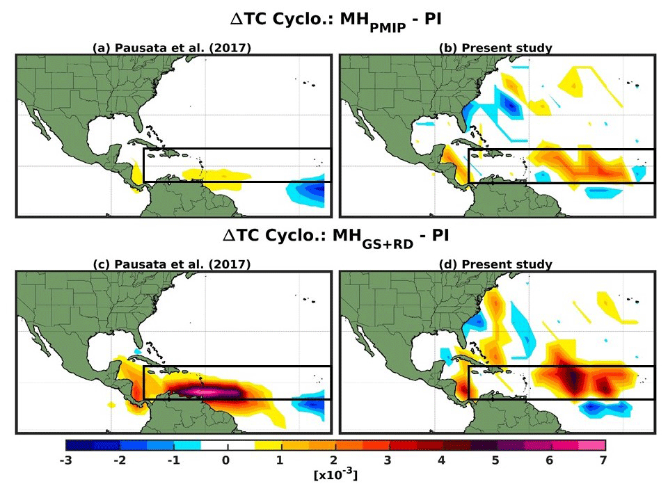
Figure A10 Comparison between TC seasonal cyclogenesis density anomalies for the (a, b) MH_PMIP and (c, d) MH_GS+RD experiments relative to PI between (a–c) Pausata et al. (2017) and (b–d) the present study. Note that data are represented over a 5^∘ mesh-grid Mercator projection in the present study, while in Pausata et al. (2017) a 4^∘ mesh grid is used to represent the fields. The black box shows the approximate present-day MDR.

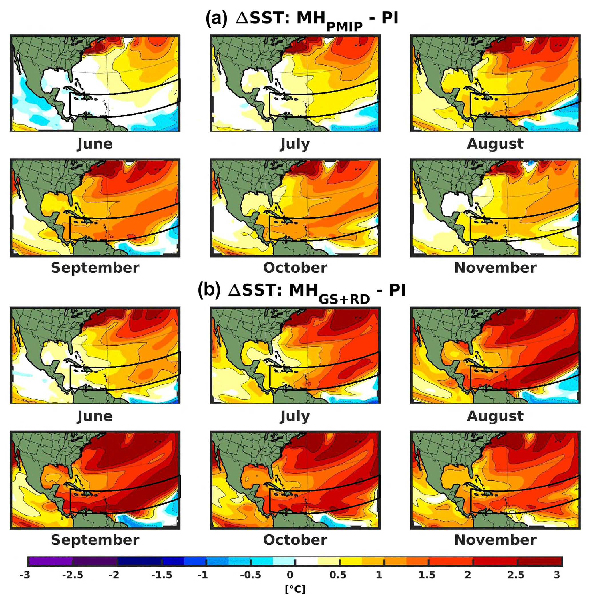
Figure A11 Monthly mean changes in climatological SSTs for the (a) MH_PMIP and (b) MH_GS+RD experiments relative to the PI experiment. The black box shows the approximate present-day MDR. Only values that are significantly different at the 5 % level using a local (grid-point) t test are shaded. The contour lines follow the color-bar scale (dashed, negative anomalies; solid, positive anomalies); the 0 line is omitted for clarity.

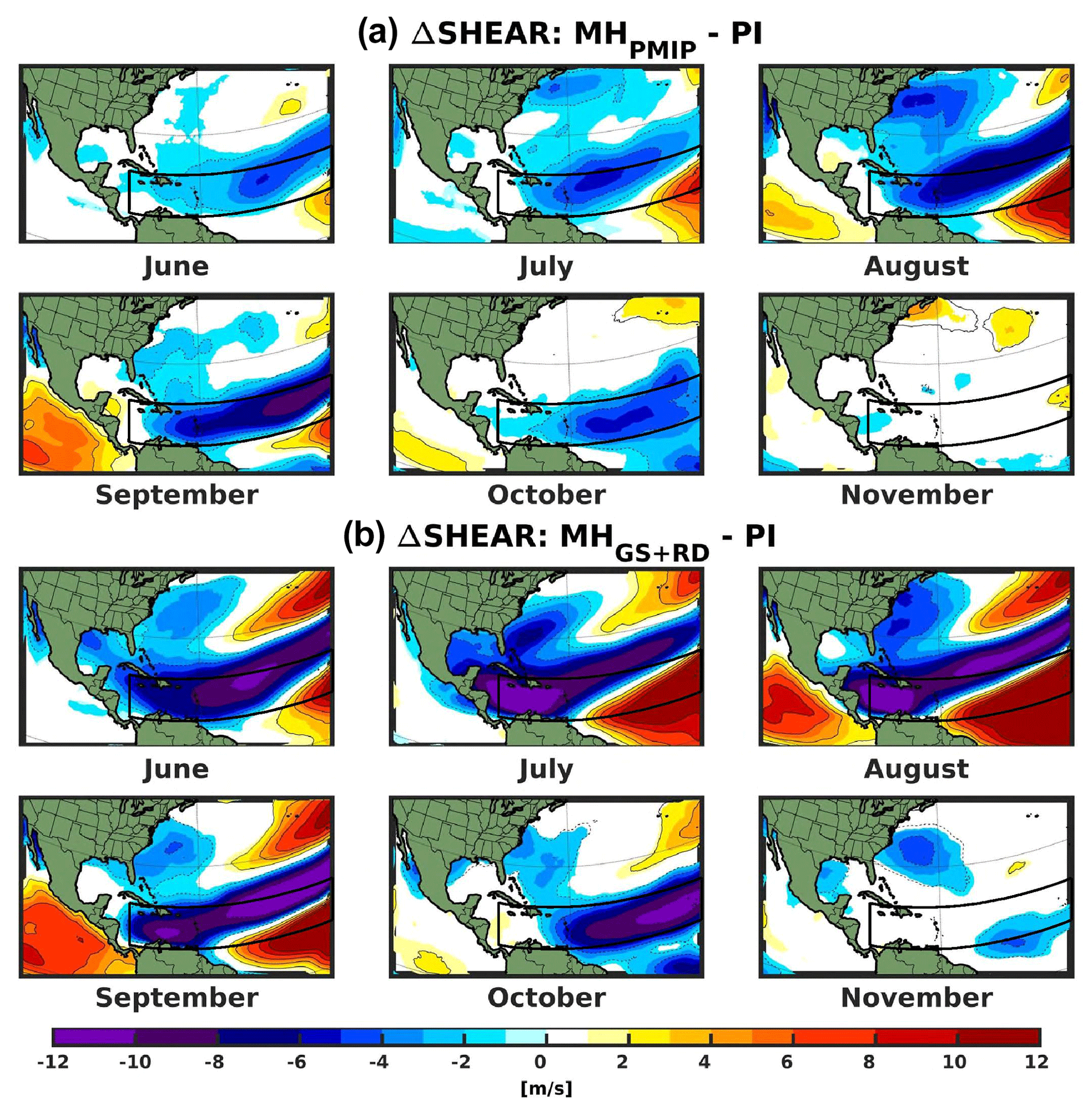
Figure A12 Monthly mean changes in climatological wind shear (200–850 hPa) for the (a) MH_PMIP and (b) MH_GS+RD experiments relative to PI. The black box shows the approximate present-day MDR. Only values that are significantly different at the 5 % level using a local (grid-point) t test are shaded. The contour lines follow the color-bar scale (dashed, negative anomalies; solid, positive anomalies); the 0 line is omitted for clarity.

Figure A13 Monthly mean changes in 850 hPa absolute vorticity for the (a) MH_PMIP and (b) MH_GS+RD experiments relative to PI. The black box shows the approximate present-day MDR. Only values that are significantly different at the 5 % level using a local (grid-point) t test are shaded. The contour lines follow the color-bar scale (dashed, negative anomalies; solid, positive anomalies); the 0 line is omitted for clarity.

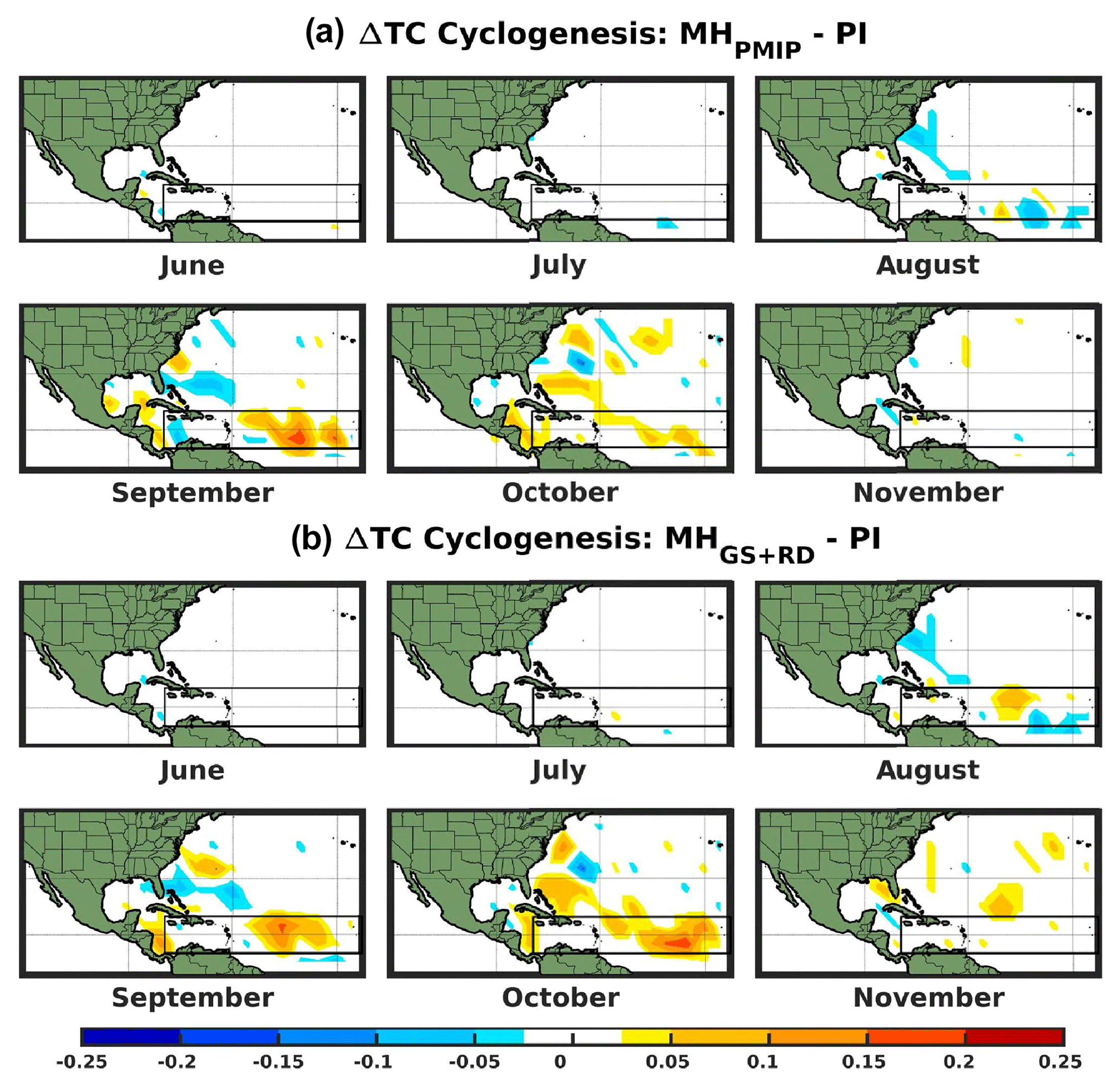
Figure A14 TC seasonal (JJASON) cyclogenesis density anomaly for the (a) MH_PMIP and (b) MH_GS+RD experiments relative to PI represented over a 5^∘ mesh-grid Mercator projection. The black box shows the approximate present-day MDR.

Figure A15 Changes in climatological seasonal CAPE between a saturated boundary layer air parcel and an air parcel that has been isothermally lowered to a reference level (JJASON) for the (a) MH_PMIP and (b) MH_GS+RD experiments relative to PI. The black box shows the approximate present-day MDR. Only values that are significantly different at the 5 % level using a local (grid-point) t test are shaded. The contour lines follow the color-bar scale with different styles (dashed, negative anomalies; solid, positive anomalies); the 0 line is omitted for clarity.