Atmospheric iron supply and marine productivity in the glacial North Pacific Ocean

Iron (Fe) is a key element in the Earth climate system, as it can enhance marine primary productivity in the high-nutrient low-chlorophyll (HNLC) regions where, despite a high concentration of major nutrients, chlorophyll production is low due to iron limitation. Eolian mineral dust represents one of the main Fe sources to the oceans; thus, quantifying its variability over the last glacial cycle is crucial to evaluate its role in strengthening the biological carbon pump. Polar ice cores, which preserve detailed climate records in their stratigraphy, provide a sensitive and continuous archive for reconstructing past eolian Fe fluxes. Here, we show the Northern Hemisphere Fe record retrieved from the NEEM ice core (Greenland), which offers a unique opportunity to reconstruct the past Fe fluxes in a portion of the Arctic over the last 108 kyr. Holocene Fe fluxes (0.042–11.7 ka, 0.5 mg m⁻² yr⁻¹) at the NEEM site were 4 times lower than the average recorded over the last glacial period (11.7–108 ka, 2.0 mg m⁻² yr⁻¹), whereas they were greater during the Last Glacial Maximum (LGM; 14.5–26.5 ka, 3.6 mg m⁻² yr⁻¹) and Marine Isotope Stage 4 (MIS 4; 60–71 ka, 5.8 mg m⁻² yr⁻¹). Comparing the NEEM Fe record with paleoceanographic records retrieved from the HNLC North Pacific, we found that the coldest periods, characterized by the highest Fe fluxes, were distinguished by low marine primary productivity in the subarctic Pacific Ocean, likely due to the greater sea ice extent and the absence of major nutrients upwelling. This supports the hypothesis that Fe fertilization during colder and dustier periods (i.e., LGM and MIS 4) was more effective in other regions, such as the midlatitude North Pacific, where a closer relationship between marine productivity and the NEEM Fe fluxes was observed.

1 Introduction

Greenland and Antarctic ice cores are unique archives that can provide records of temperature, atmospheric dust load and atmospheric gas composition variability during the Holocene and the late Pleistocene (Jouzel et al., 1996; Lambert et al., 2008; Schüpbach et al., 2018; Watanabe et al., 2003). Glacial periods were dustier and were characterized by a lower CO₂ concentration (≈ 180 ppm) than interglacials (≈ 280 ppm) (Lambert et al., 2008; Lüthi et al., 2008). This dichotomy is explained through several different hypotheses: the increase in aridity and newly exposed continental shelves (Fuhrer et al., 1999), an increase in the aerosol atmospheric lifetime resulted from a reduced hydrological cycle (Lambert et al., 2008; Yung et al., 1996), increased glacial-derived mobilization of highly bioavailable iron (Fe) from physical breakdown of bedrock (Shoenfelt et al., 2018), and, lastly, more vigorous polar circulation capable of entraining additional dust from lower latitudes (Mayewski et al., 1994). Regardless of the source, the higher atmospheric burden of mineral dust during glacial periods affected climate through both physical and biological mechanisms. Dust particles can directly influence the Earth's radiative budget by scattering, absorbing and re-emitting shortwave and longwave radiation (Miller and Tegen, 1998; Schepanski, 2018). During the Last Glacial Maximum (LGM), model results showed that the enhanced dust transport alone caused a 1.0 W m⁻² globally averaged radiative forcing decrease compared with present-day conditions, which contributed to a 0.85 ^∘C cooling relative to the current climate (Mahowald et al., 2006). Conversely, once deposited on the ocean surface, the mineral dust delivered major and micronutrients (including Fe) that could have stimulated the biological carbon pump (Martin et al., 1990). Indeed, Fe can limit marine primary production (MPP) in the high-nutrient low-chlorophyll (HNLC) oceans, which are characterized by a high concentration of nutrients but low productivity (Martin et al., 1990). The largest (HNLC) oceans are the Southern Ocean, the equatorial Pacific and the North Pacific Ocean (Duggen et al., 2010). In these regions, the Fe role in modulating marine productivity has been demonstrated through both artificial Fe fertilization experiments (Smetacek et al., 2012; Tsuda et al., 2003; Yoon et al., 2018) and natural Fe inputs from iceberg melting, volcanic eruptions and glacially sourced dust (Duprat et al., 2016; Langmann et al., 2010; Shoenfelt et al., 2017). For its biological relevance, it has been hypothesized that the recorded decrease in the atmospheric CO₂ concentration during glacial periods was linked to the Fe-modulated enhancement of the biological carbon pump in the HNLC regions due to the increase in Fe availability (Martin et al., 1990). Evidence of the existence of a strong link between atmospheric Fe deposition and marine productivity was retrieved from a marine sediment core collected in the subantarctic zone of the Southern Ocean, where the coldest periods were mirrored by an increase in atmospheric Fe fluxes and by an enhancement in both MPP and the degree of nutrient consumption (Martínez-García et al., 2014). Yet, according to both modeling (Lambert et al., 2015) and observational (Gaspari et al., 2006; Röthlisberger et al., 2004; Vallelonga et al., 2013) studies, the Fe fertilization mechanism itself cannot completely explain the ≈ 100 ppmv glacial–interglacial atmospheric CO₂ variability, only accounting for around 8–20 ppmv of it (Lambert et al., 2015).

However, the role of Fe fertilization in the Northern Hemisphere and in the HNLC region of the North Pacific is unclear due to the few available Arctic Fe flux records, which are either limited to the last century or only cover short time periods (Burgay et al., 2019; Hiscock et al., 2013). Thus, reconstructing how the Fe concentrations and fluxes have changed in the Northern Hemisphere during the last glacial cycle is essential in order to understand the evolution of the global atmospheric circulation, the human impact on dust mobilization (Mahowald et al., 2008) as well as to evaluate the impact that Fe might have had on MPP in the North Pacific HNLC region. Here, we present a high-resolution 108 kyr record of total dissolvable Fe (TDFe) retrieved from the North Greenland Eemian Ice Drilling (NEEM) ice core (Rasmussen et al., 2013; Schüpbach et al., 2018), which provides a unique insight into the atmospheric Fe supply in the Arctic both during the Holocene and the last glacial period. Furthermore, we performed a comparison between the TDFe NEEM record and various paleoproductivity records from the HNLC North Pacific region (Fig. 1) to evaluate whether the increase in eolian Fe fluxes was mirrored by an increase in marine productivity. We underline that the TDFe concentration, as it will be discussed in the following, derives from the acidification of the snow samples for 1 month at pH 1. Thus, the values represent an upper limit of the eolian Fe potentially available for the phytoplankton, and they might overestimate the actual bioavailable Fe.

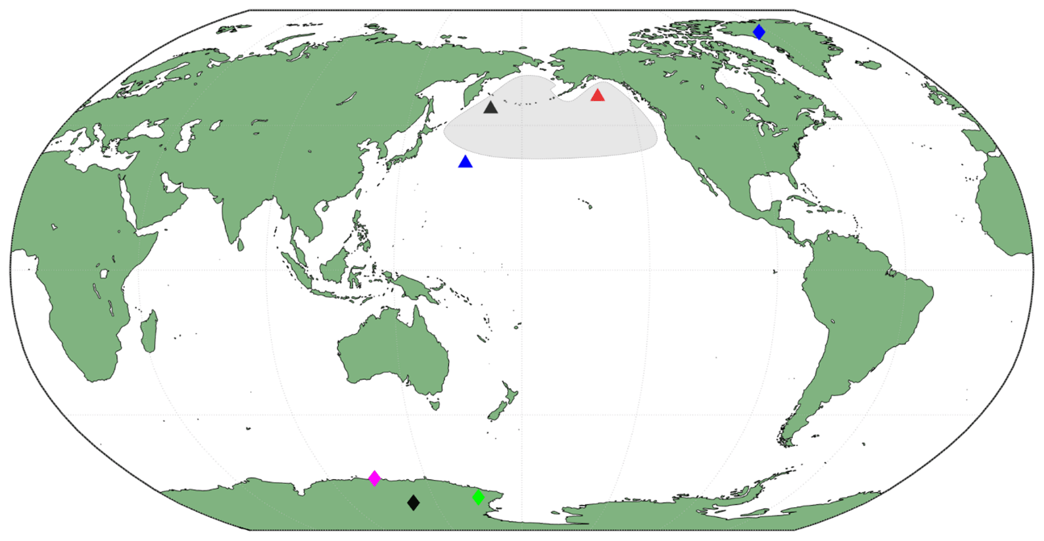
Figure 1 Location of the NEEM ice core (blue diamond; this study), the LD ice core (pink triangle; Edwards et al., 2006), the EDC ice core (black diamond; Wolff et al., 2006) and the TD ice core (green diamond; Vallelonga et al., 2013). We retrieved paleoproductivity data for the eastern North Pacific (black triangle) from the ODP882 (Haug et al., 1995) and SO202-27-6 (Méheust et al., 2018) sediments cores, and we retrieved these data for the western Pacific Ocean (red triangle) from the ODP887 (McDonald et al., 1999) and SO202-07-6 (Méheust et al., 2018) sediment cores. The paleoproductivity record from the midlatitude North Pacific was retrieved from the S-2 sediment core (blue triangle; Amo and Minagawa, 2003).

2 Materials and methods

2.1 Sampling and processing

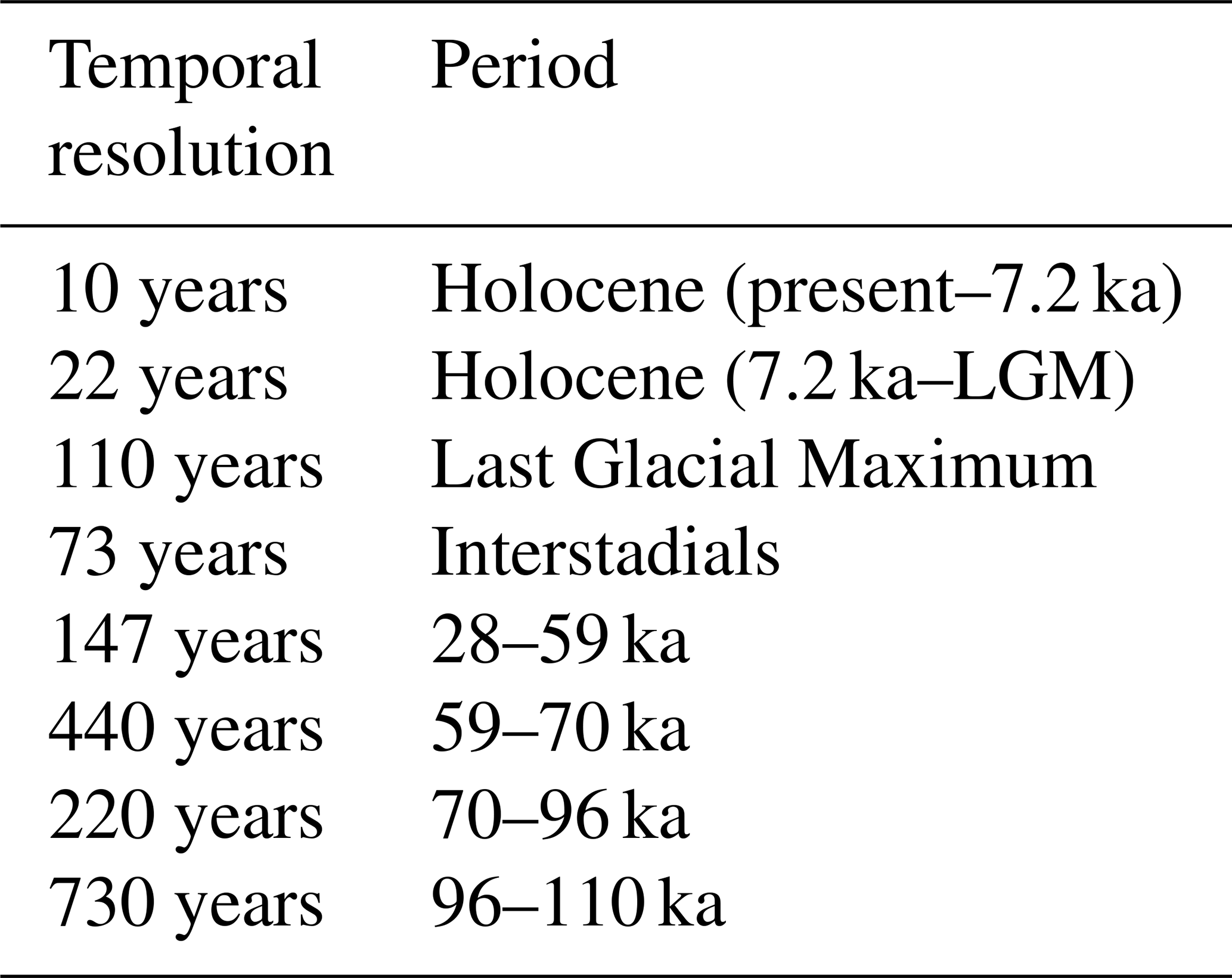
In the framework of the NEEM project, a 2540 m deep ice core was drilled in northwestern Greenland (77^∘45^′ N, 51^∘06^′ W) at 2479 m a.s.l. The site is characterized by an average annual temperature of −29 ^∘C and a modern accumulation of 22 cm ice equivalent per year. According to the GICC05modelext-NEEM-1 timescale, the ice core covers the last 128 kyr (Rasmussen et al., 2013). The ice cores were cut to obtain ice sticks with a square cross section of 36 mm × 36 mm. They were continuously melted on a continuous flow analysis (CFA) system with a typical melt speed of 3.5 cm min⁻¹ (Schüpbach et al., 2018). The CFA system provides meltwater from the inner and least likely to be contaminated part of the core; thus, we did not adopt any further decontamination procedure. The inductively coupled plasma mass spectrometry (ICP-MS) samples were manually collected at a low resolution (110 cm). The temporal resolution depends on the accumulation rate and decreases with depth because of the ice thinning. According to the available timescale (Rasmussen et al., 2013) and considering the 110 cm sampling resolution, the temporal resolution varies from decadal to millennial (Table 1).

Table 1 Temporal resolution of the NEEM ice core in accordance with the GICC05modelext-NEEM-1 age scale (Rasmussen et al., 2013). Ice samples for ICP-MS analysis were collected with a resolution of 110 cm.

Samples were collected in vials that had been previously cleaned as follows: stored in HNO₃ 5 % for 7 d (Suprapure, ROMIL, UK), rinsed three times with ultrapure water (UPW, ELGA, UK), stored in HNO₃ 2 % for 7 d (Suprapure, ROMIL, UK), rinsed three times with UPW and then stored in HNO₃ 1 % (Ultrapure, ROMIL, UK) until the day before the sample collection, when they were rinsed three times with UPW and dried overnight under a laminar flow hood (Class 100). The samples were kept frozen and shipped to Italy for analysis. Once melted, the samples were acidified to pH 1 using HNO₃ (Suprapure, ROMIL, UK). To ensure an effective dissolution of Fe particles, samples were stored at room temperature and analyzed 30 d after the acidification without any additional filtration step. We adopted this approach because analysis immediately after the acidification step might have led to uncertainties attributable to the Fe dissolution kinetics (Edwards, 1999; Koffman et al., 2014). Our choice was consistent with other studies that have indicated that samples to be used for the calculation of atmospheric fluxes must be acidified for at least 1 month prior to analysis in order to avoid any possible misinterpretation of the trace element data (Koffman et al., 2014). We will refer to this fraction as total dissolvable Fe (TDFe); total dissolvable Fe includes both the most labile fraction (dissolved iron, DFe), which is rendered soluble under mildly acidic conditions (Hiscock et al., 2013), and the fraction enclosed in iron-bearing mineral particles. TDFe does not directly represent the actual bioavailable Fe that can be dissolved into seawater at pH 8, but, considering that TDFe and DFe are significantly correlated (Du et al., 2020; Xiao et al., 2020), it represents an upper limit of the eolian Fe potentially available for the phytoplankton (Edwards et al., 2006).

2.2 Analytical procedure and performances

The ice samples were analyzed with an Inductively Coupled Plasma Single Quadrupole Mass Spectrometer (ICP-qMS, Agilent 7500 series, USA) equipped with a quartz Scott spray chamber for the determination of Ca, Na and Fe. To minimize any kind of contamination, all of the instrument tubes were flushed before the analysis for 2 h with 2 % HNO₃ (Suprapure, ROMIL, UK). A 120 s rinsing step with 2 % HNO₃ (Suprapure, ROMIL, UK) occurred after each sample analysis to reduce any possible memory effect. The vials used for the standard preparation were cleaned following the same procedure adopted for the ice samples. Considering the isobaric and polyatomic interferences affecting Fe, this element was quantified using the interference-free isotope ⁵⁷Fe. External calibration curves with acidified standards (2 % HNO₃, Suprapure, ROMIL, UK) were prepared for Ca, Na and Fe from the dilution of a certified single-element 1000 ppm ± 1 % standard solution (Fisher Chemical, USA). The resulting R² for the external calibration curves was 0.999 for all of the elements. The limit of detection (LoD) for ⁵⁷Fe, calculated as 3 times the standard deviation of the blank, was 0.8 µg L⁻¹. To assess accuracy for Fe, the TM-RAIN04 certified reference material (National Research Council of Canada) was measured every 50 samples. The accuracy was determined as a recovery percentage calculated as $O/T$ %, where O is the determined value, and T is the certified value. For Fe, the accuracy was 104 %, whereas precision, calculated as relative standard deviation (RSD %) of selected samples read multiple times (n = 5) during the analysis, was on average 5 % (7 % for samples (n = 3) from the interglacial period, and 4 % for samples (n = 3) from the last glacial period). For Ca and Na, the LoD was 1 and 3 µg L⁻¹, respectively. In the absence of a certified reference material, Ca and Na accuracy was calculated using a quality control (QC) sample prepared at 10 µg L⁻¹ and measured every 50 samples. Accuracy for Ca and Na, calculated as described above, was 94 % and 108 %, respectively, whereas precision (RSD %) was on average 6 % (4 % for samples from the interglacial period, and 7 % for samples from the last glacial period) and 2 % (for both periods), respectively.

The non-sea-salt Ca concentration is commonly used as proxy for terrestrial inputs in polar regions, and it is calculated as nssCa = [Ca] − ([Ca] $/$ [Na])_sw ⋅ [Na], where “sw” indicates seawater.

3 Results and discussion

3.1 Fe fluxes from the NEEM core

Fe and nssCa concentrations and fluxes were calculated as $F=C\cdot A$, where F is the Fe flux (in mg m⁻² yr⁻¹), C is the Fe or nssCa concentration (in ng g⁻¹) and A the accumulation (in m yr⁻¹ ice equivalent) previously determined by Rasmussen et al. (2013). A pattern of higher dust (expressed as nssCa²⁺) and Fe fluxes during colder climate periods and lower dust and Fe fluxes during warmer climate periods is clearly recognizable (Fig. 2, Table 2).

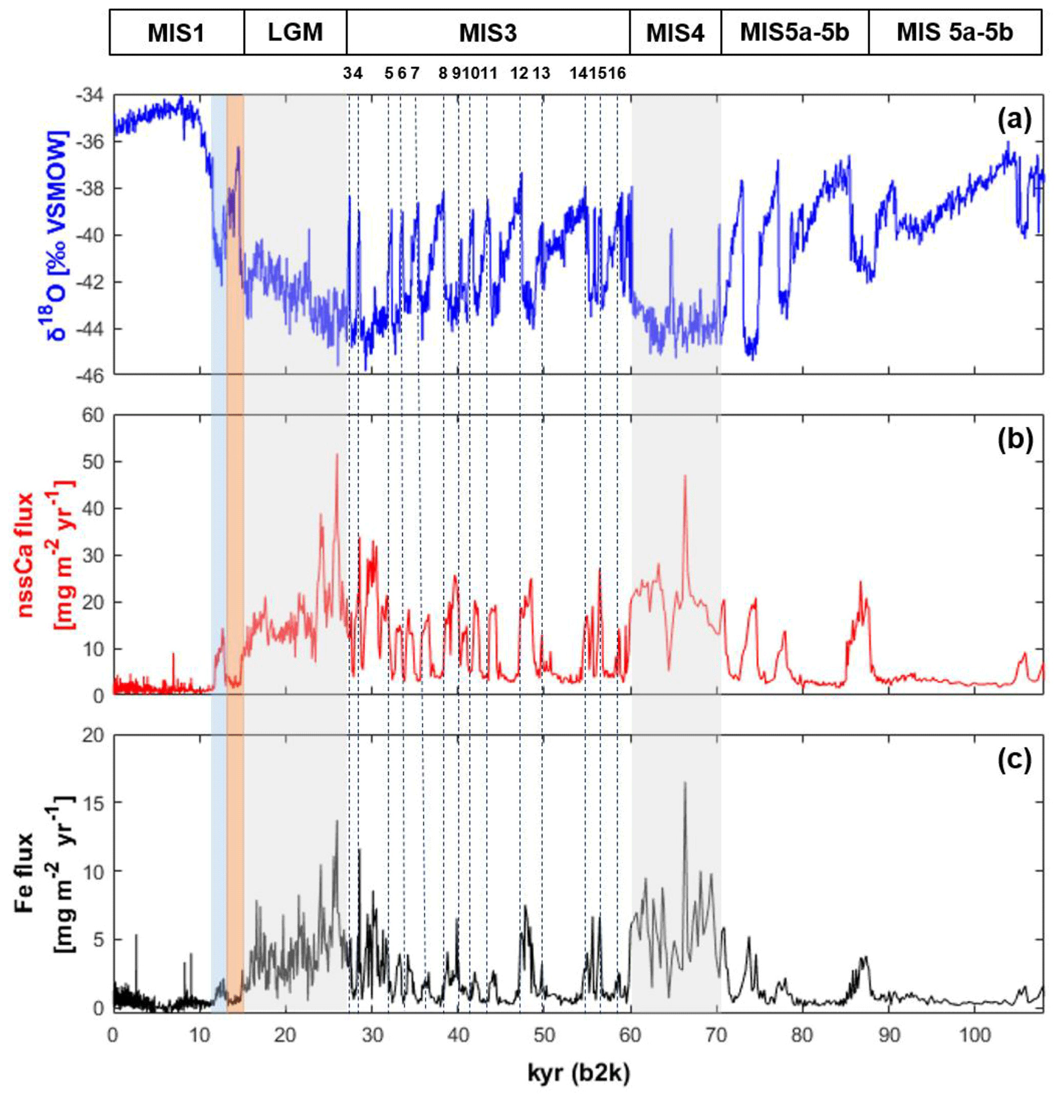
Figure 2 (a) The δ¹⁸O (blue line) profile from the NGRIP ice core (North Greenland Ice Core Project Members, 2007). (b) The nssCa flux (red line) from the NEEM ice core, and (c) the Fe flux (black line) from the NEEM ice core. The shaded blue rectangle denotes the Younger Dryas, and the shaded orange rectangle denotes the Bølling–Allerød. The numbers above panel (a) indicate the Dansgaard–Oeschger events from 3 to 16.

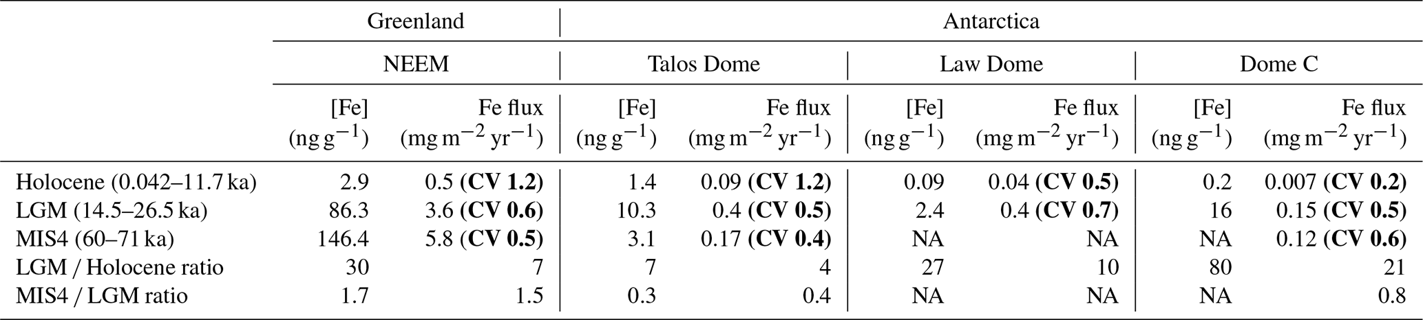
Table 2 Fe and nssCa average concentrations (ng g⁻¹) and fluxes (mg m⁻² yr⁻¹) from the NEEM ice core. More details are given in the text. The coefficient of variability (CV) was calculated for Fe and nssCa fluxes and is reported in bold.

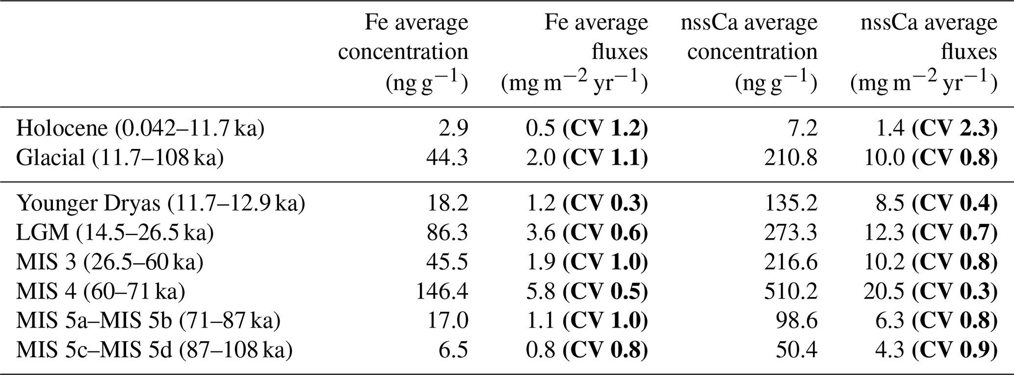
The Holocene (0.042–11.7 ka) was characterized by average Fe fluxes of 0.5 mg m⁻² yr⁻¹ that varied between 0.01 and 5.3 mg m⁻² yr⁻¹ (Fig. 2). The coefficient of variability (CV), calculated as the ratio between the standard deviation and the mean value, was 1.2. The more recent 4000 years are characterized by the highest average Fe fluxes (0.6 ± 0.4 mg m⁻² yr⁻¹). The lowest Fe fluxes were recorded between 4000 and 8000 years b2k (0.3 ± 0.2 mg m⁻² yr⁻¹). During the Younger Dryas (YD; 11.7–12.9 ka), an abrupt cooling was observed with a drop in the δ¹⁸O value from −36.9 ‰ to −43.1 ‰. Coincidently, the recorded average Fe fluxes rose to 1.2 ± 0.4 mg m⁻² yr⁻¹, higher than both the 12.9–13.9 ka (0.5 ± 0.3 mg m⁻² yr⁻¹) and the 10.7–11.7 ka (0.3 ± 0.2 mg m⁻² yr⁻¹) periods.

The last glacial period (11.7–108 ka) showed Fe fluxes 4 times higher (2.0 ± 2.2 mg m⁻² yr⁻¹) than the Holocene, spanning from 0.05 to 16.5 mg m⁻² yr⁻¹ (Fig. 2). However, a significant variability during the last glacial period was detected. During the LGM and MIS 4, average Fe fluxes were 7 times (3.6 ± 2.3 mg m⁻² yr⁻¹) and 10 times (5.8 ± 2.8 mg m⁻² yr⁻¹) greater than the Holocene average. Fe fluxes also increased during the MIS 5c–MIS5b transition (87 ka), when a concurrent decrease in δ¹⁸O values was observed. During MIS 5c and MIS 5d, Fe fluxes were comparable with those detected during the Holocene. The high frequency of the Dansgaard–Oeschger (D–O) events during MIS 3 was mirrored by the high variability in both nssCa and Fe fluxes. Each stadial period corresponded to an increase in both Fe and nssCa. However, their variability was significantly different. During MIS 3, Fe fluxes showed maximum values greater than 5 mg m⁻² yr⁻¹ during D–O 4, 9, 12 and 15 (8.5, 6.5, 7.5 and 6.6 mg m⁻² yr⁻¹ respectively), and lower than 5 mg m⁻² yr⁻¹ during D–O 6, 7, 8, 10, 11 and 13 (3.9, 2.6, 4.1, 2.6, 2.7 and 3.2 mg m⁻² yr⁻¹ respectively). This variability was significantly higher than that recorded for nssCa, which showed maximum values close to 20 mg m⁻² yr⁻¹ for all of the D–O events.

3.2 Comparison with Fe fluxes from Antarctic ice cores

The NEEM Fe ice core record allows for the first comparison of Fe concentrations and fluxes between the Arctic and Antarctica (Fig. 3, Table 3). The only Antarctic Fe records that can reach at least the LGM are from Talos Dome (TD) (Spolaor et al., 2013; Vallelonga et al., 2013), Law Dome (LD) (Edwards et al., 2006; Edwards et al., 1998) and EPICA Dome C (EDC) (Wolff et al., 2006). However, we point out that both the samples from Dome C and Talos Dome were acidified for at least 24 h, leading to a possible underestimation of the actual TDFe concentration. This implies that the general trends and features can be comparable with the NEEM record, whereas absolute concentrations might differ due to the different acidification procedure used (Koffman et al., 2014).

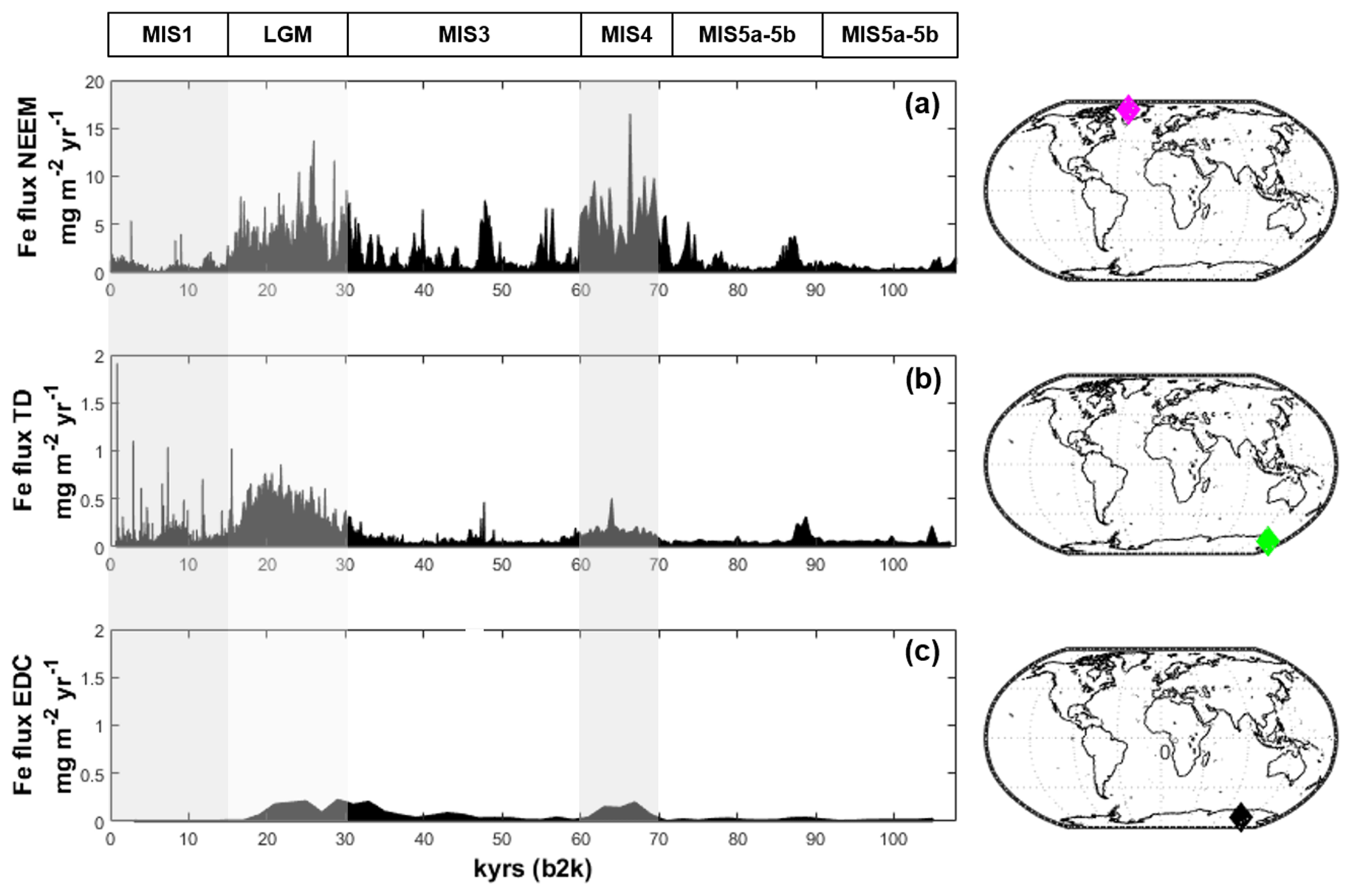
Figure 3 Comparison of the Fe fluxes among (a) NEEM (pink diamond; this work), (b) TD (green diamond; Vallelonga et al., 2013) and (c) EDC (black diamond; Wolff et al., 2006). Note that the y axis for NEEM ranges from 0 to 20 mg m⁻² yr⁻¹, whereas the y axis for TD and EDC ranges from 0 to 2 mg m⁻² yr⁻¹.

Table 3 Comparison of the average Fe concentration ([Fe], in ng g⁻¹) and fluxes (in mg m⁻² yr⁻¹) among four different ice cores: NEEM, Talos Dome (Vallelonga et al., 2013), Law Dome (Edwards et al., 2006) and Dome C (Wolff et al., 2006). NA stands for not available. The average Fe concentration at DC is not available, as the accumulation rate at that site during MIS4 is unavailable. Data from Law Dome span from 59 to 8.5 ka (for the Holocene) and from 18.2 to 23.7 ka (for the LGM). The coefficient of variability (CV) was calculated for Fe fluxes and is reported in bold for all of the cores.

In Antarctica, the average Fe flux and concentration values varied significantly among the different sites during the Holocene with similar values recorded at the coastal sites (TD) and lower values recorded in the internal Antarctic Plateau (EDC) (Table 3). For TD, this was explained both through changes in atmospheric transport patterns across Antarctica and through an additional local input of dust from proximal Antarctic ice-free zones that affected coastal sites more than the central plateau, which was exclusively exposed to remote sources such as southern South America (Albani et al., 2012; Delmonte et al., 2010b; Vallelonga et al., 2013).

During the LGM, both TD and EDC shared a similar dust flux loading, comprised between 10 and 15 mg m⁻² yr⁻¹ (Baccolo et al., 2018), and the same dust source region, as confirmed by the Sr–Nd isotopes (Delmonte et al., 2010a). Compared with the Holocene, the atmospheric dust fluxes in TD increased by a factor 6, whereas the increase was by approximately a factor 25 in EDC (Delmonte et al., 2010b). This is mirrored by a similar average Fe flux enhancement compared to the Holocene with values that were up to 4- and 21-fold higher, respectively (Vallelonga et al., 2013; Wolff et al., 2006). These discrepancies between the two sites are likely due to the higher Holocene dust flux observed in TD compared with EDC, as a consequence of a relevant local dust contribution at TD (Baccolo et al., 2018; Delmonte et al., 2010b).

During the last glacial period, the most relevant dust source was southern South America for both TD and EDC (Basile et al., 1997; Delmonte et al., 2010b; Lambert et al., 2008). Dust fluxes peaked during MIS 4 where both sites recorded maximum values around 10 mg m⁻² yr⁻¹ (Lambert et al., 2008; Vallelonga et al., 2013) and comparable Fe fluxes (0.17 ± 0.07 mg m⁻² yr⁻¹ at TD and 0.12 ± 0.07 mg m⁻² yr⁻¹ at EDC) (Vallelonga et al., 2013; Wolff et al., 2006).

The LD record, due to the different analytical preparation of the samples, is not directly comparable with TD and EDC. Nevertheless, we can still evaluate and discuss the Fe flux ratio between the Holocene and the LGM. Unfortunately, for the LD record, there is no dust profile available, meaning that it is not possible to define the main dust and Fe sources for this location, although the Australian continent has been an important source of mineral dust in the recent past (Edwards et al., 2006; Vallelonga et al., 2002). During the LGM, Fe fluxes increased 10-fold compared with the Holocene period, 2.5 times more than what was observed in TD. Similarly to what was observed in the EDC record, this difference might be explained by the absence of local dust sources that affected LD during the Holocene or by the lower sampling frequency for the LD record (n = 27) compared with TD (n = 801).

Despite the different acidification times, the overall picture during the Holocene is that the average Fe fluxes in NEEM (0.5 mg m⁻² yr⁻¹, CV = 1.2) were higher than in Antarctica. Among the Antarctic Fe fluxes, TD (0.09 mg m⁻² yr⁻¹, CV = 1.2) and LD (0.04 mg m⁻² yr⁻¹, CV = 0.5) were higher than those recorded at EDC (0.007 mg m⁻² yr⁻¹, CV = 0.2).

In NEEM, the LGM (19–26.5 ka) was characterized by a 10-fold and 7-fold enhancement in dust (expressed as nssCa) and Fe fluxes, respectively. A similar behavior was observed in the Antarctic cores as described above (Table 3). Considering that the atmospheric CO₂ concentration dropped down to 180 ppm (Köhler et al., 2017), the global Fe flux enhancement likely contributed to part of this decrease, promoting marine productivity in some HNLC regions (Amo and Minagawa, 2003; Kawahata et al., 2000; Martínez-Garcia et al., 2011).

During MIS 4 (60–71 ka), NEEM Fe fluxes were higher than all of the other investigated records. Compared with the LGM average, dust (Ruth, 2007), nssCa and Fe fluxes (this work) in the Arctic during MIS 4 exhibited a ≈ 1.5-fold increase (Table 3), while they were lower both in TD and EDC. To explain this behavior we advance some hypotheses. The first is that the increase in dust and Fe fluxes can be attributable to changes in the atmospheric circulation, likely due to the topographic influence of the Laurentide Ice Sheet (LIS). Indeed, during the LGM, the LIS was nearly 2 times larger than at MIS 4 (Löfverström et al., 2014; Tulenko et al., 2020), and it might have caused a stronger meridional splitting of the westerlies (Löfverström et al., 2014) and a southward migration of their mean position (Kang et al., 2015; Manabe and Broccoli, 1985). The southward shift during the LGM might have produced a reduction in strong winds passing over the source areas (i.e., Taklimakan and Gobi deserts) (Kang et al., 2015) and/or a stronger southward Fe and dust deposition over the Chinese Loess Plateau (Zhang et al., 2014) and the midlatitude North Pacific (Sun et al., 2018). In contrast, during MIS 4, the westerlies might have been located northward (i.e., over the Taklimakan and Gobi deserts) and characterized by a less marked meridional splitting (Löfverström et al., 2014), conveying a larger amount of dust to Greenland. We also propose two alternative hypotheses that rely on (1) the possibility that additional dust sources (e.g., Saharan dust) might have reached Greenland during MIS 4 and on the fact that (2) during MIS 4, the Asian monsoon system was stronger in winter than in summer, producing drier conditions that caused an enhanced dust production and transport to Greenland (Xiao et al., 1999). However, to better address this point, a more comprehensive investigation that involves a large set of paleorecords and atmospheric modeling is required, although this is beyond the scope of this paper.

3.3 Comparison with lower-resolution Fe NEEM measurements

A parallel study that reported the Fe concentration from the NEEM ice core was recently published (Xiao et al., 2020). It reports the TDFe and DFe concentrations and fluxes with a lower temporal resolution (n = 166) than the current investigation (n = 1596). Moreover, the analytical approach was different, as the melted ice samples were filtered at 0.45 µm and acidified for 6 weeks before the analysis. Even though the overall pattern between the two records is similar, we observe several differences between Xiao et al. (2020) and our study: (a) the average Fe concentration over the entire record is 4-fold higher than that found in our investigation (101.4 ng g⁻¹ vs. 20.4 ng g⁻¹); (b) the Fe concentration range is wider (1.5–1194.5 ng g⁻¹ vs. > LoD – 457.6 ng g⁻¹) compared with the data presented in this paper; (c) average Fe fluxes are 2.4-fold higher during the Holocene (1.2 mg m⁻² yr⁻¹ vs. 0.5 mg m⁻² yr⁻¹) and 3.5-fold higher during the LGM (12.5 mg m⁻² yr⁻¹ vs. 3.6 mg m⁻² yr⁻¹) compared with those recorded in this study; (d) the LGM Fe flux showed a 10-fold increase during the Holocene, compared with the 7-fold enhancement that we observed; (e) the TDFe fluxes and concentrations were higher during the LGM than during MIS 4, whereas we found higher fluxes during MIS 4, consistent with a similar enhancement of nssCa and dust (Ruth, 2007).

Possible reasons for these differences might stem from the different temporal resolution and the discrepancies between the adopted analytical approaches; this highlights the need to standardize the analytical procedures when trace elements are analyzed in ice and snow samples in order to have a more reliable comparison among both different and identical locations.

3.4 Fe and marine productivity in the Northern Hemisphere

Considering the biological relevance of Fe and taking advantage of the Fe flux record retrieved from the NEEM ice core, one important question remains regarding whether its flux increase during the last glacial period triggered the marine productivity in the HNLC region of the North Pacific (Olgun et al., 2011).

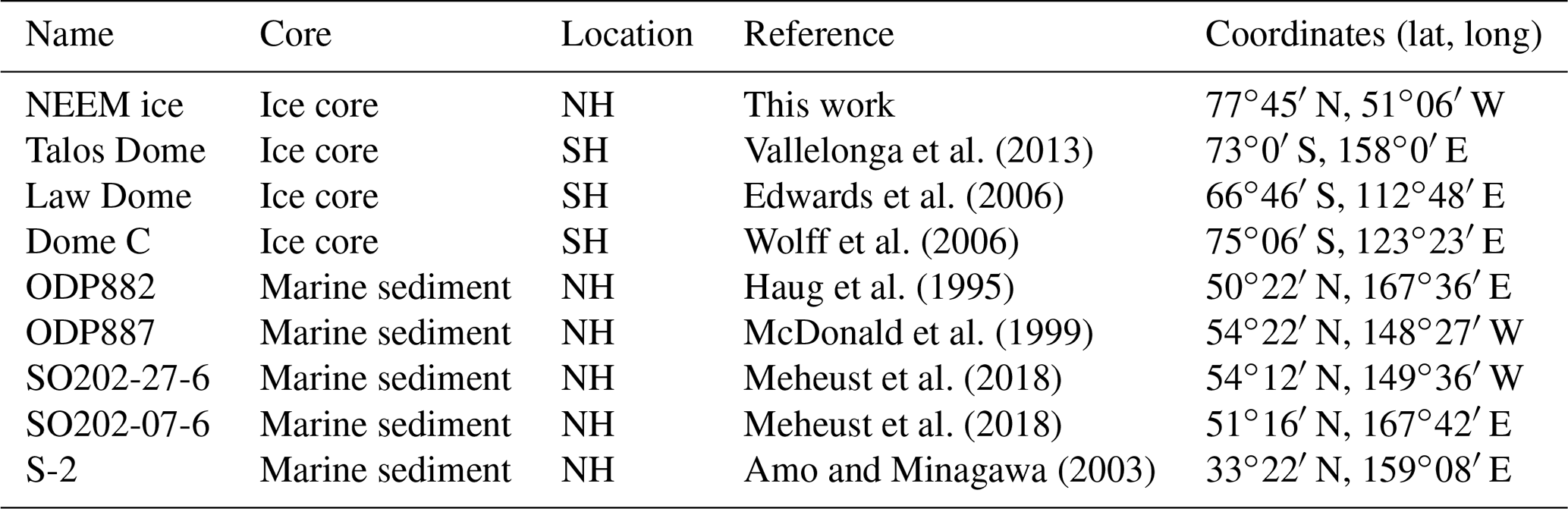
Table 4 Summary of locations and data sources for all the cores (both ice and sediment cores) discussed in the text. (NH stands for Northern Hemisphere, and SH stands for Southern Hemisphere.)

Nowadays, a significant amount of Asian dust (250 Mt yr⁻¹) is primarily deposited over the HNLC region of the subarctic Pacific (Serno et al., 2014; Zhang et al., 2003), and the marine productivity changes in this oceanic region might reflect potential Fe fertilization effects promoted by atmospheric Fe supply. During modern times, both increases in the eolian influx from Asia (Young et al., 1991) and sporadic Fe input from volcanic eruptions (Langmann et al., 2010) have resulted in an enhancement of MPP by more than 60 %. Moreover, recent Fe fertilization experiments performed south of the Gulf of Alaska (McDonald et al., 1999; Tsuda et al., 2003) have shown significant increases in the abundance of diatoms and in the chlorophyll-a concentration (Boyd et al., 1996), indicating that the North Pacific is possibly sensitive to atmospheric Fe inputs. However, no data are available to evaluate if the Fe sensitivity of the subarctic Pacific Ocean holds over even longer timescales or if an increase in the eolian Fe supply, observed during glacial periods, could explain the MPP variability in the subarctic Pacific Ocean. To address these points, we compared the NEEM Fe record with different marine sediment cores (Table 4).

For both interglacial and glacial periods, previous geochemical evidence indicates that the dust source influencing Greenland and the North Pacific mainly originated from the East Asian deserts (Schüpbach et al., 2018; Serno et al., 2014). However, considering that there are no eolian Fe flux records from the marine sediment cores, they might have received different amount of Fe compared with what is observed in the ice core record. Through a comparison between a marine sediment record from the western subarctic Pacific Ocean (SO202-07-6) and the NGRIP ice core, it has been shown that dust fluxes changed coherently and simultaneously during abrupt climate changes, although the amplitude of the change was different (Serno et al., 2015). The larger variability observed in NGRIP, as well as in NEEM, compared with marine sediments indicates changes in the atmospheric dust transport from the source areas to Greenland (e.g., rate of aerosol rainout and different wind strength).

Recently, it has been proposed that additional dust sources might have influenced Greenland in the last 31 kyr (Han et al., 2018; Lupker et al., 2010). Strontium and lead isotopes indicate that Saharan dust contributed to the overall NEEM dust budget during the Younger Dryas (12 %–73 %) and between 17 and 22 ka (16 %–70 %), while the Taklimakan and Gobi contribution (i.e., eastern Asia sources) was dominant (55 %–94 %) prior to 22 ka (Han et al., 2018). However, despite the Saharan dust source, we assume that the main dust source for the NEEM ice core during the last glacial period is represented by the Gobi and Taklimakan deserts (Svensson et al., 2000). This is coherent with the dust changes' synchronicity among Greenland, the Chinese loess (Ruth et al., 2007) and the northern Pacific sediment records located downwind of the Asian dust sources (Schüpbach et al., 2018; Serno et al., 2015). Nevertheless, additional investigations to assess the magnitude of the Saharan dust contribution prior to 31 ka and to identify other possible source regions are needed.

All variables considered (i.e., different dust amplitude and other potential dust sources), and observing that the overall pattern of higher dust deposition during the coldest periods is consistent between the ice and sediment core records, we assumed that the Fe flux changes observed in NEEM are representative for the eolian Fe supply to the subarctic Pacific Ocean.

Figure 4 Comparison between Fe fluxes (black line, a) from NEEM (pink diamond; this work) and marine productivity (red line, b) from ODP887 in the eastern subarctic Pacific (green triangle; McDonald et al., 1999), ODP882 (red line, c) in the western subarctic Pacific (black triangle; Haug et al., 1995) and S-2 (red line, d) in the midlatitude North Pacific (red triangle; Amo and Minagawa, 2003). Due to their limited temporal extension, productivity records from SO202-07-6 and SO202-07-26 are not discussed in this figure and are instead shown in Fig. 5.

To evaluate whether past marine productivity was influenced by the atmospheric Fe supply for the period ranging from the LGM to the Holocene, we compared the NEEM record with the high temporal resolution SO202-27-6 (from the Patton–Murray Rise plateau, eastern subarctic Pacific Ocean) and the SO202-07-6 (from the Detroit Seamount, western subarctic Pacific Ocean) productivity records (Méheust et al., 2018). For a long-term record, we relied on the ODP887 (McDonald et al., 1999) and the ODP882 (Haug et al., 1995) sediment cores, located close to SO202-27-6 and SO202-07-6, respectively. A comparison over the last 108 kyr between the NEEM record and the S-2 sediment core (from the Shatsky Rise, midlatitude North Pacific) was also performed (Amo and Minagawa, 2003) (Fig. 4, Table 4).

The past marine primary productivity reconstruction was performed relying on the $\mathrm{Si}/\mathrm{Al}$ ratio, the percentage of biogenic silica and the brassicasterol concentration. The $\mathrm{Si}/\mathrm{Al}$ ratio is used as a proxy for opal, or biogenic silica (diatoms), in the absence of directly measured opal concentrations. The normalization to Al removes any possible variable inputs of lithogenic detritus (McDonald et al., 1999). Brassicasterol is a sterol compound that has been used as a molecular indicator of the presence of diatoms (Sachs and Anderson, 2005). The brassicasterol concentration is also used, along with highly branched isoprenoid alkenes (IP₂₅), for the phytoplankton IP₂₅ index (PIP₂₅) calculation, which is a proxy for the evaluation of past sea ice conditions (Méheust et al., 2018; Müller et al., 2011)

3.4.1 From the LGM to the Holocene

During the Last Glacial Maximum, the Fe fluxes recorded in the NEEM ice core were 7 times higher than during the Holocene. However, marine productivity in the subarctic Pacific Ocean, expressed as the $\mathrm{Si}/\mathrm{Al}$ ratio (McDonald et al., 1999), the percentage of biogenic silica (Haug et al., 1995) and the brassicasterol concentration (Méheust et al., 2018), was at its lowest level (Figs. 4, 5). Reconstructions based on the foraminifera-bound δ¹⁵N (FB-δ¹⁵N), a proxy which indicates the degree of nitrate consumption by phytoplankton (Martínez-García et al., 2014), showed that, in the western subarctic Pacific Ocean, the nitrate consumption was more complete during the LGM and the YD (i.e., when MPP was low) compared with the warmest periods (Ren et al., 2015). In other words, during the coldest and dustiest periods, the nitrate consumption efficiency was higher (i.e., increase in the FB-δ¹⁵N values) than during the interglacials, even though MPP was low. This apparent contradiction can be explained by an increase in water stratification (either by reduced upwelling or vertical mixing), where the most nutrient-rich and oxygen-depleted waters were shifted to deeper depths, whereas nutrient-depleted and better-ventilated waters rested above a hydrographic boundary at 1500–2000 m (Kohfeld and Chase, 2017). Water stratification led to the minimal input of nutrients to the surface ocean, leading the system towards a major nutrient limitation (Kienast et al., 2004; Ren et al., 2015). Among the several possible reasons that can explain the increase in water stratification in the glacial North Pacific, we propose two hypotheses. The first relies on the glacial closure of the Bering Strait that reduced the freshwater export from the Pacific Ocean to the Atlantic, retaining more freshwater in the North Pacific (Talley, 2008). The second involves sea ice formation. When sea ice forms, in the Okhotsk and Bering seas, brine rejection occurs, increasing water density and creating the more saline and denser North Pacific Intermediate Water (NPIW). When the wind blows the sea ice away from where it was originally formed, brine rejection can further proceed at the same location following the formation of new sea ice. The continuous brine rejection promotes the freshening of surface waters and strengthens water stratification (Costa et al., 2018).

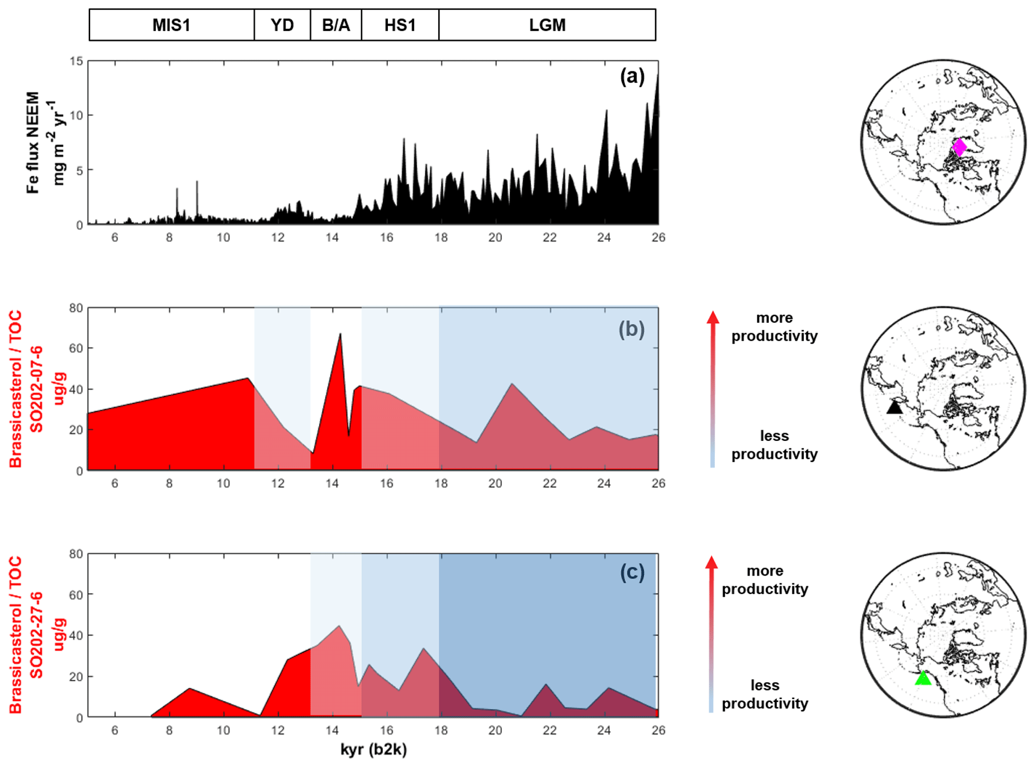
Figure 5 Relationship between the Fe flux in the NEEM core and MPP in subarctic Pacific Ocean over the last 26 kyr, where a higher brassicasterol–total organic carbon ratio represents an increase in productivity. Sea ice data are from Meheust et al. (2018): prevalently extended sea ice (dark blue rectangle), prevalently marginal sea ice (blue rectangle), prevalently variable sea ice (light blue rectangle) and prevalently ice-free (white rectangle). The Fe flux record (black line, a), productivity in the eastern subarctic Pacific Ocean (SO202-07-6, red line, b) and productivity in the western subarctic Pacific Ocean (S0202-27-6, red line, c) are also shown. Productivity pulses were recorded when sea ice changed its conditions towards ice-free conditions. YD stands for Younger Dryas, B/A stands for Bølling–Allerød, HS1 stands for Heinrich Stadial 1 and LGM stands for Last Glacial Maximum.

An additional explanation for the observed lower productivity during glacial periods arises from the higher extent of perennial sea ice that might have played a role in creating a physical barrier between the atmosphere and the marine environment, reducing the amount of available sunlight and the direct deposition of bioavailable Fe on the seawater surface (Kienast et al., 2004; Méheust et al., 2018). Marine sediment records, collected in the eastern and western subarctic Pacific and in the Bering Sea, have shown extended spring ice cover during the LGM (Méheust et al., 2018; Méheust et al., 2016) when the Fe fluxes were at their maxima. The progressive decrease in perennial sea ice coverage recorded after the LGM led to an increase in the marine productivity (Fig. 5), with a maximum during the Bølling–Allerød (B/A) warm event (≈ 13–15 kyr ago). The possible relevance of sea ice in modulating MPP at the highest latitude of the Pacific Ocean during the LGM is strengthened by a marine sediment record collected in the midlatitude North Pacific (Amo and Minagawa, 2003), which, because of its southernmost location, did not experience any sea ice condition. During the LGM, contrarily to what is observed in the subarctic Pacific, a prominent maximum in marine productivity was recorded, suggesting that Fe could have triggered an important phytoplankton response (Fig. 4d). The Fe sensitivity of the midlatitude North Pacific is confirmed during the Holocene, when the Fe fluxes were at their minima and the productivity, expressed as MAR (mass accumulation rate) C₃₇ alkenone (µg cm⁻² kyr⁻¹), was at its lowest level. A plausible explanation is that stratified waters did not characterize this region during the last glacial period and, thus, it was not affected by the limitation of major nutrients. Unfortunately, neither FB-δ¹⁵N nor information about water stratification is available for this record.

However, there might be other reasons that could explain the strengthening in MPP during the B/A warm period in the subarctic North Pacific. Among them, we propose the increase in the sea level that inundated previously exposed lands which might have entrained iron and other nutrients to the marine ecosystem (Davies et al., 2011), or changes in the oceanic circulation (McManus et al., 2004). Indeed, at the onset of the B/A event, the meridional overturning circulation rapidly accelerated, and this might have produced an upward displacement of the nutrient-rich North Pacific Deep Water towards intermediate depths, promoting an injection of nutrients to surface waters and enhancing marine productivity.

These additional explanations shed light on the marginal role that atmospheric Fe fertilization had in promoting MPP in the subarctic Pacific Ocean, as other players might have had a more significant impact (Kohfeld and Chase, 2017).

3.4.2 From 108 ka to the LGM

According to the available records, marine productivity changed heterogeneously in the Pacific Ocean during the last glacial period (Fig. 4).

It is challenging to state, with a high degree of confidence, whether or not Fe fertilization triggered a phytoplankton bloom in the HNLC subarctic North Pacific. This is due to the different responses that the western and the eastern side of the subarctic North Pacific showed with respect to the atmospheric Fe supply (Fig. 4). In the eastern subarctic Pacific, the increase in the eolian Fe fluxes was mirrored by a phytoplankton response during the MIS 5.2 and the MIS 5–MIS 4 transition. The subsequent decrease in MPP during the MIS 4 suggests that the prolonged Fe supply during the coldest stadial might have led the ecosystem towards the limitation of other nutrients (Kienast et al., 2004), following the same mechanisms described in the previous section. The enhanced water stratification during those periods, as suggested by stable oxygen isotope ratios in planktonic foraminifera (Zahn et al., 1991), did not allow a supply of macronutrients from below the mixed layer. Thus, the additional atmospheric Fe supply had little effect on phytoplankton productivity, suggesting their growth was likely limited by the lack of major nutrients (Kienast et al., 2004). In the western subarctic Pacific, the increase in productivity was also recorded in periods with low atmospheric Fe fluxes (e.g., from 100 to 90 ka at ODP882), strengthening the hypothesis that other influences (e.g., meltwater inputs, continental margin supply and sea ice) had a more relevant role (Kienast et al., 2004; Lam and Bishop, 2008) than the atmospheric Fe supply.

Contrary to what was observed in the subarctic Pacific, the S-2 sediment core collected in the midlatitude North Pacific (Amo and Minagawa, 2003) showed a marked increase in MPP during MIS 4 and the overall last glacial period when the Fe fluxes were higher (Fig. 4). MPP in the midlatitude North Pacific might have been more sensitive to the atmospheric Fe supply, suggesting that the high degree of upper-ocean stratification that characterized the subarctic region of the Pacific Ocean did not affect the midlatitude North Pacific, allowing for a continuous supply of macronutrients. The observed increase in dust transport (and Fe deposition) could have then stimulated marine productivity (Kienast et al., 2004).

4 Conclusions and future perspectives

In this study, we provided a high temporal resolution Fe record from mineral dust input retrieved from the NEEM ice core. Through the comparison with other available Fe records, we observed that Fe fluxes were higher in Greenland than in Antarctica. The greatest difference between the Arctic and Antarctic records occurred during MIS4, when Fe fluxes in NEEM were 1.5 times higher than during the LGM, whereas, in TD and EDC, they were lower. To explain this behavior, we advanced two hypotheses (i.e., change in the atmospheric circulation or additional dust sources that reached Greenland), although more detailed investigations are needed.

Merging our record with marine productivity data, we found that a link between Fe transport and ocean productivity holds in the midlatitude North Pacific, indicating that this area might be sensitive to the atmospheric Fe supply. On the contrary, in the subarctic Pacific, we did not find any overwhelming evidence that the increase in the atmospheric Fe fluxes triggered a phytoplankton response. This indicates that other players, such as sea ice and increased water stratification during the coldest periods, had a more relevant role in modulating MPP in the HNLC region of the North Pacific on a millennial timescale.

This study provides an upper limit for estimating the potentially bioavailable Fe supplied to marine phytoplankton in the North Pacific region; however, additional studies should focus on analyzing the labile and bioavailable Fe fractions to constrain the realistic Fe supply and response of the marine ecosystem.