the Creative Commons Attribution 4.0 License.
the Creative Commons Attribution 4.0 License.
 | 03 Dec 2021
Climate and ecology in the Rocky Mountain interior after the early Eocene Climatic Optimum
Rebekah A. Stein
Sarah E. Allen
Michael E. Smith
Rebecca M. Dzombak
Brian R. Jicha
As atmospheric carbon dioxide (CO2) and temperatures increase with modern climate change, ancient hothouse periods become a focal point for understanding ecosystem function under similar conditions. The early Eocene exhibited high temperatures, high CO2 levels, and similar tectonic plate configuration as today, so it has been invoked as an analog to modern climate change. During the early Eocene, the greater Green River Basin (GGRB) of southwestern Wyoming was covered by an ancient hypersaline lake (Lake Gosiute; Green River Formation) and associated fluvial and floodplain systems (Wasatch and Bridger formations). The volcaniclastic Bridger Formation was deposited by an inland delta that drained from the northwest into freshwater Lake Gosiute and is known for its vast paleontological assemblages. Using this well-preserved basin deposited during a period of tectonic and paleoclimatic interest, we employ multiple proxies to study trends in provenance, parent material, weathering, and climate throughout 1 million years. The Blue Rim escarpment exposes approximately 100 m of the lower Bridger Formation, which includes plant and mammal fossils, solitary paleosol profiles, and organic remains suitable for geochemical analyses, as well as ash beds and volcaniclastic sandstone beds suitable for radioisotopic dating. New 40Ar 39Ar ages from the middle and top of the Blue Rim escarpment constrain the age of its strata to ∼ 49.5–48.5 Myr ago during the “falling limb” of the early Eocene Climatic Optimum. We used several geochemical tools to study provenance and parent material in both the paleosols and the associated sediments and found no change in sediment input source despite significant variation in sedimentary facies and organic carbon burial. We also reconstructed environmental conditions, including temperature, precipitation (both from paleosols), and the isotopic composition of atmospheric CO2 from plants found in the floral assemblages. Results from paleosol-based reconstructions were compared to semi-co-temporal reconstructions made using leaf physiognomic techniques and marine proxies. The paleosol-based reconstructions (near the base of the section) of precipitation (608–1167 mm yr−1) and temperature (10.4 to 12.0 ∘C) were within error of, although lower than, those based on floral assemblages, which were stratigraphically higher in the section and represented a highly preserved event later in time. Geochemistry and detrital feldspar geochronology indicate a consistent provenance for Blue Rim sediments, sourcing predominantly from the Idaho paleoriver, which drained the active Challis volcanic field. Thus, because there was neither significant climatic change nor significant provenance change, variation in sedimentary facies and organic carbon burial likely reflected localized geomorphic controls and the relative height of the water table. The ecosystem can be characterized as a wet, subtropical-like forest (i.e., paratropical) throughout the interval based upon the floral humidity province and Holdridge life zone schemes. Given the mid-paleolatitude position of the Blue Rim escarpment, those results are consistent with marine proxies that indicate that globally warm climatic conditions continued beyond the peak warm conditions of the early Eocene Climatic Optimum. The reconstructed atmospheric δ13C value (−5.3 ‰ to −5.8 ‰) closely matches the independently reconstructed value from marine microfossils (−5.4 ‰), which provides confidence in this reconstruction. Likewise, the isotopic composition reconstructed matches the mantle most closely (−5.4 ‰), agreeing with other postulations that warming was maintained by volcanic outgassing rather than a much more isotopically depleted source, such as methane hydrates.
- Article
(19639 KB) - Full-text XML
-
Supplement
(3427 KB) - BibTeX
- EndNote


1.1 The Eocene period as an analog for a future warm world
The anthropogenic release of fossil fuels drives a rapid and sustained increase in atmospheric carbon dioxide (CO2) that is coupled with climate change (Bernstein et al., 2007). To understand the effects of elevated CO2 on the Earth (e.g., Cotton et al., 2013), we seek out geological periods with high temperatures and high atmospheric CO2 for comparison. The early Eocene Climatic Optimum (EECO) has been invoked as a climate analog for our projected future (e.g., Zhu et al., 2019). This warming during the EECO occurred 53.26–49.14 million years ago (Cramwinckel et al., 2018; Westerhold et al., 2018), with peak warming from 51.5–50.9 Ma; this period consisted of long-term global temperature maxima and high CO2 levels but was tectonically comparable to today (Hyland and Sheldon, 2013; West et al., 2020). From the Paleocene to early Eocene, it has been inferred that there were extensive temperate forests dispersed throughout North America (Smith et al., 2012; Breedlovestrout et al., 2013; Greenwood et al., 2016; West et al., 2020) up to high latitudes at 65∘ N (Dillhoff et al., 2013). However, the nearby Bighorn Basin is inferred to have undergone aridification based on magnetic properties in paleosols (Maxbauer et al., 2016; Carmichael et al., 2017), and global climate models predict low- and lower–middle-latitude sites, including areas like central Utah, to experience aridification due to changes in meridional vapor transport distribution (Pagani et al., 2006). As the planet warms, there is increasing concern about water availability and dry climates getting drier. For example, the North American Southwest, composed of a series of deserts and dry ecosystems, is at risk of having its already severe droughts increase in frequency and severity (Poore et al., 2005; Coats et al., 2015; Cheeseman, 2016). Therefore, the study of ancient climate and ecosystems in these hydrologically vulnerable areas can provide examples for what may happen to these ecosystems in the context of emerging climate and societal challenges.
1.2 Continental interior and foreland basins in the Rocky Mountains
The marine foreland of the North American Cordillera was partitioned into a series of terrestrial basins by an anastomosing network of Laramide basement structures during the Paleogene, likely due to coupling between the shallow Farallon slab with the North American lithosphere (Dickinson et al., 1988; Snoke et al., 1993; DeCelles, 2004). Geomorphic evolution of drainage patterns during the Paleocene and Eocene that were driven by Laramide orogenesis led to the formation of a series of large lakes, preserved as several kilometers of lacustrine and fluvial strata (Smith et al., 2008). High sediment accumulation rates in these basins contributed locally to excellent preservation of the biota, allowing us to study deep time at high resolution (Looy et al., 2014). The carbonate-rich lacustrine Green River Formation was deposited from Lake Gosiute within the greater Green River Basin (Fig. 1). The predominantly siliciclastic Wasatch and Bridger formations reflect contemporaneous fluvial and floodplain deposition adjacent to Lake Gosiute.
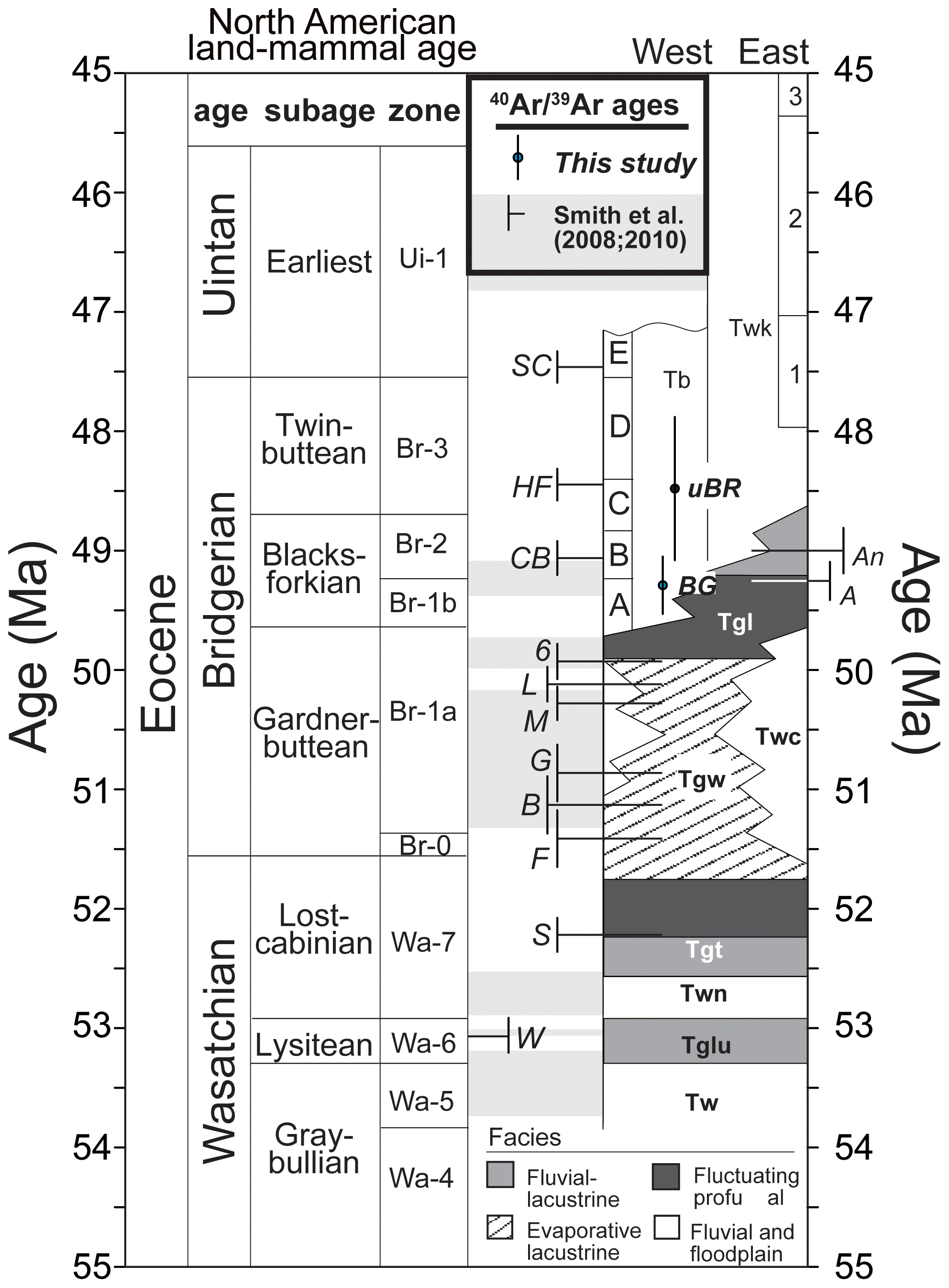
Figure 1Age model of Eocene Wyoming. The North American land mammal age (NALMA) is shown for context. The upper Blue Rim is shown as “uBR”, the blue–green marker is depicted as “BG”, and both are shown with dots and error bars. Dates from M. E. Smith et al. (2008, 2010) are shown in perpendicular lines. The abbreviations included are designated as follows. Green River Formation: Tglu – Luman Member, Tgt – Tipton Member, Tgl – Laney Member. Wasatch Formation: Tw – “main body,” Twn – Niland Tongue, Twc – Cathedral Bluffs Member, Tb – Bridger Formation, Twk – Washakie Formation. Tuff beds as measured in M. E. Smith et al. (2008, 2010) are denoted as follows. W: Willwood, S: Scheggs, R: Rife, F: Firehole, B: Boar, G: Grey, M: Main, L: Layered, 6: Sixth, A: Analcite, CB: Church Butte, HF: Henry's Fork, and SC: Sage Creek.
The greater Green River Basin lies to the east of the Sevier fold-and-thrust belt and is bounded on the north, east, and south by Laramide basement structures, each of which likely contributed water and sediment to the basin (Smith et al., 2008, 2014). The basin also likely received water and sediment at times from paleoriver(s) which drained the high-elevation Cordilleran hinterland to the west (Chetel and Carroll, 2010; Chetel et al., 2011; Smith et al., 2014). Over 2 km of terrestrial strata accumulated in it depocenter during the Paleogene. The paleolatitude of southwestern Wyoming in the early Eocene (∼ 41∘ N; Wolfe et al., 1998; Hyland and Sheldon, 2013) is thought to be relatively comparable to its position today, and thus changes in the climate of this region are not related to changes in latitude.
1.3 Using multiple proxies to characterize an environment
High-resolution, well-informed snapshots in time of individual regions with thorough climate reconstructions help us to understand climate change and subsequent ecosystem dynamics (Guiot et al., 2009; Li et al., 2010; Shala et al., 2017). There are several terrestrial proxies that can be used to reconstruct paleoclimate and paleoecology, e.g., pedogenic carbonate isotope values (Cerling, 1992), floral assemblages (Wilf, 2000; Spicer et al., 2009), and stomatal density (Royer, 1999). The preservation of abundant, high-quality organic and inorganic specimens and samples due to the tectonic assemblage of the basin makes the Green River Basin (GGRB) an excellent location for a multi-proxy approach. Organic geochemistry, specifically isotopic values of plants (δ13Cplant), has been used to reconstruct the value of the isotopic composition of the atmosphere – termed δ13Catm (Arens et al., 2000; Stein et al., 2019). δ13Catm reflects sources of CO2 gas to the atmosphere (Keeling, 1979; Boutton, 1991); for example, mantle degassed values of δ13Catm tend to be around −5.4 ‰ (Deines, 1992). Identifiable organic fossils with individually compressed leaves can be used to reconstruct the value of the atmosphere. Multiple inorganic geochemistry proxies (see methods) can provide context for the depositional environment (e.g., Sheldon et al., 2006), climate (e.g., Gallagher and Sheldon, 2013), hydroclimate (e.g., Sheldon et al., 2002), age (e.g., Turner, 1971), and origin of sediments (e.g., Sheldon and Tabor, 2009). Together, these proxies can inform us on ecosystem and depositional dynamics in the context of Eocene climate. This study seeks to combine these proxies to create a holistic reconstruction of the greater GGRB during the early Eocene using the extensive deposits of the Blue Rim escarpment.
The Bridger Formation is an approximately 842 m thick series of tuffaceous deltaic–alluvial and minor lacustrine sedimentary strata which overlie and interfinger with the Green River Formation (Koenig, 1960; Kistner, 1973; Murphey, 2001; Murphey and Evanoff, 2011; Clyde et al., 2001). Vertebrate fossils collected from the Bridger Formation formed the basis for defining the Bridgerian North American land mammal “age” (NALMA; e.g., Osborn, 1909; Wood et al., 1941; Van Houten, 1944; Gingerich et al., 2003; Robinson et al., 2004). Mapping and biostratigraphy have permitted further subdivision of the Bridger Formation into intervals A–E (Matthew, 1909; Murphey and Evanoff, 2011; Murphey et al., 2011). Several volcanic ash horizons within the Bridger Formation and the underlying Green River Formation have been radioisotopically dated using 40Ar 39Ar geochronology to have accumulated between approximately 50 and 46 Ma (Fig. 1; Table S2; Murphey and Evanoff, 2011; Smith et al., 2008). Radioisotopic ages reported or discussed in this contribution have all been calculated using the 28.201 Ma age for the Fish Canyon tuff sanidine standard and are thus comparable with modern U–Pb geochronology (Kuiper et al., 2008; M. E. Smith et al., 2010). Strata exposed along the Blue Rim study area represent the oldest exposed portion of the Bridger Formation. Unlike much of the Bridger Formation, these “Bridger A” deposits have not been radioisotopically dated, but regional mapping and correlations suggest they were deposited above the Sand Butte bed of the Laney Member of the Green River Formation and likely occur beneath the more extensively mapped Bridger B interval (Murphey, 2001; Murphey and Evanoff, 2011), bracketing a depositional age between the ca. 50 Ma “sixth tuff” of the Green River Formation and the ca. 49 Ma age for the Church Butte tuff, which occurs within Bridger B (Fig. 1).
Several potential sediment sources may have contributed to the Bridger Formation, including siliciclastic material of a variety of compositions derived from Phanerozoic strata and underlying basement exposed by Laramide uplifts which surround the basin (Smith et al., 2015), volcaniclastic and siliciclastic sediment delivered by the Idaho paleoriver (Chetel et al., 2011), volcanic ashfall from the Challis and Absaroka volcanic fields, and autochthonous lacustrine carbonates (Murphey and Evanoff, 2011; Fig. 1a). Evidence supporting these as potential sources include common detrital feldspar ages in the sand grains that are similar to depositional ages (i.e., recently erupted volcanic grains) and many euhedral volcanic biotite and felsic volcanic lithic grains in the Bridger Formation sandstones (Chetel et al., 2011). Whereas the older, and in part coeval, Laney Member of the Green River Formation is composed primarily of carbonate lacustrine sediments, the Bridger Formation is composed principally of siliciclastic sediment, with several minor intervals of lacustrine carbonate (Buchheim et al., 2000; Murphey and Evanoff, 2011). Sediment accumulation during Bridger Formation deposition appears to have been relatively continuous in the basin center based on existing age control (Murphey and Evanoff, 2011). Because of this, the Bridger Formation has pristine faunal and floral preservation, making it an excellent candidate for understanding ecosystem function (Brand et al., 2000; Allen et al., 2015; Allen, 2017b).
The Bridger Formation is exposed laterally over 12 km at Blue Rim and is locally approximately 100 m thick (Kistner, 1973). The flora at Blue Rim has been collected and described in great depth and is known for excellent plant preservation including leaves, flowers, fruits, seeds, wood, pollen, and spores (Allen, 2017a, b). Eocene floral assemblages at Blue Rim occupy warm, wet biomes not unlike modern subtropical ecosystems; angiosperms including palms were abundant and dicotyledonous taxa were up to 28 m tall (Allen, 2015, 2017a, b), antithetical to the dry scrub desert found at the Blue Rim escarpment today. Of the multiple quarries created for plant fossil excavation (see Allen, 2017a, b), the lower horizon (older) floral assemblage consists of taxa such as the abundant climbing fern Lygodium kaulfussi (fern, Lygodiaceae), “dicots” like Serjania rara (soapberry, Sapindaceae), Populus cinnamomoides (poplar, Salicaceae), and Landeenia arailiodes (Sapindales, Goweria bluerimensis (Icacinaceae), and Phoenix windmillis (palm; Arecaceae; Allen, 2015; Allen et al., 2015; Allen, 2017b). The upper horizon preserves taxa such as Macginitiea wyomingensis (sycamore; Platanaceae), Populus cinnamomoides (poplar, Salicaceae), Cedrelospermum nervosum (elm; Ulmaceae), Serjania rara (soapberry, Sapindaceae), and many more (Allen, 2017b).
3.1 Geochronology
Volcaniclastic beds were sampled from the Blue Rim escarpment for 40Ar 39Ar geochronological dating (e.g., Turner, 1971): two samples from the prominent “blue–green marker” unit (Fig. 3, 31 m in Figs. 4–7) that occurs approximately halfway up the section and two sand beds that crop out near the top of the exposure. To prepare sanidine phenocrysts for analysis, samples were crushed, leached in dilute hydrochloric acid (HCl) and hydrofluoric acid (HF) prior to hand-picking of sanidine in refractive index oils using a petrographic microscope, and then ultrasonically cleaned in acetone and ethanol. Sanidine phenocrysts from sampled ash beds were irradiated adjacent to standard sanidine crystals from Fish Canyon tuff (FCs) in cadmium shielding within the TRIGA (Training, Research, Isotopes, General Atomics) water-cooled, low-enriched uranium–zirconium fuel reactor at Oregon State University. Single sanidine crystals were fused using a 25W CO2 laser and then analyzed for 40Ar 39Ar composition using a MAP 215-50 mass spectrometer attached to a metal ultrahigh-vacuum (UHV) gas extraction and clean-up line at the University of Wisconsin Madison WiscAr laboratory. A 28.201 Ma age for Fish Canyon sanidine standard (FCs; Kuiper et al., 2008) was used to calculate apparent ages for each laser fusion analysis, and weighted mean ages were calculated for the youngest coherent population of sanidine dates from each sample. For populations that exceed a mean square weighted deviation (MSWD) of 1, uncertainties in the weighted mean were multiplied by the inverse of the square root of the MSWD to reflect the additional uncertainty implied by the associated age scatter.
3.2 Physical measurements
3.2.1 Stratigraphy and fossils
Starting at the base of the Blue Rim escarpment, adjacent to the first sampled paleosol (Fig. 2), an updated stratigraphic column to that found in Allen's (2017b) dissertation was measured (41.7985∘ N, −109.5856∘ E) in September 2019 (Figs. 3, 4, 5, 6, 7). This 67 m stratigraphic column traced the flanks of the escarpment to the top of the badlands. The stratigraphic column was sampled every 3 m (approximately the height of two Jacob staffs) or at every interval of visual change (color, texture). In addition, plant fossils and plant hash were quarried at two locations approximately halfway (26, 33 m) and close to the top of the stratigraphic section (51.5, 52 m) for organic-rich fossil samples for isotope and bulk chemistry analysis.
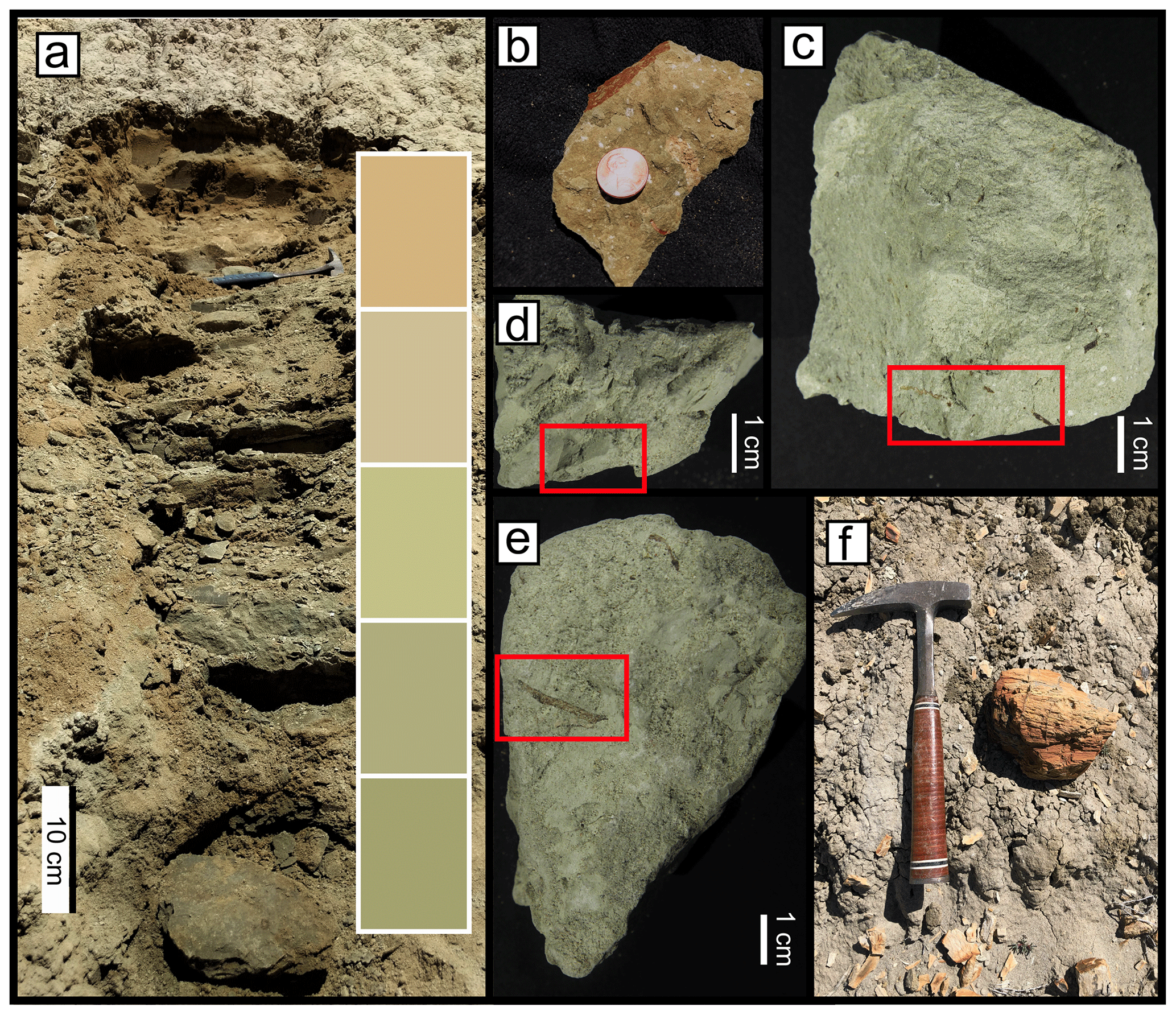
Figure 2Paleosol images and features. (a) Full profile of 19BRWY3 with a rock hammer for scale, (b) drab-haloed root trace from 19BRWY-2UB, (c) A-horizon fine organic rootlets in red box from 19BRWY2UA, (d) slickensides on 19BRWY1UA, (e) rhizoliths from 19BRWY1UA, and (f) mineralized wood with a rock hammer for scale, excavated ∼ 3 m above 19BRWY1.

Figure 3Map and profile of the Blue Rim escarpment. (a) Landscape image of the escarpment from the uppermost strata. (b) Location of the Blue Rim escarpment (blue square) at present in the context of the present tectonic configuration of the world using a Robinson projection map. (c) Shaded relief map of the North American Cordillera showing the paleogeographic position of the Blue Rim (BR) relative to major paleorivers, lake basins, and tectonic elements. EC refers to early Bridgerian Elderberry Canyon local fauna of Emry (1990). Core complexes occur near the Cordilleran paleodivide: B – Bitterroot; A – Anaconda; W – Wildhorse; G – Albion–Raft River–Grouse Creek; S – Snake. Note that the Bridger Formation at Blue Rim represents the topsets of the Sand Butte delta (see Smith et al., 2008). Paleorivers are summarized from Henry et al. (2012), Dickinson et al. (2012), and Chetel et al. (2011).
3.2.2 Paleosol sampling
Six profiles of the same paleosol were identified and excavated along a lateral transect at the base of the Blue Rim escarpment (41.79892625, −109.58362614, WGS 1984 – 19BRWY1; Figs. 7, S8). Paleosols were sampled by horizon based on pedogenic features including root traces, burrows, drab-haloed and kerogenized roots, and horizonation (Fig. S1a, Table S1). Fresh rock material was excavated by digging at least 20 cm into the surface, avoiding all traces of modern pedogenesis or surficial climate influence (i.e., modern roots or carbonate nodules). One distinctive, laterally continuous paleosol at the base of the section was sampled in five individual profiles over 440 m (Figs. 3, S1, S2, 19BRWY2-6). Samples were collected from each horizon present, with no fewer than three samples per paleosol profile. At each location, every present horizon (A, B, C) was sampled. Epipedons were present for all paleosols except 19BRWY4. For horizons that had color, texture, and/or other physical intra-horizonal changes, multiple samples were collected.
3.2.3 Isotope analyses
Paleosol samples were ground to 70 µm in a shatterbox. Approximately 10 g aliquots of samples were weighed out and then acidified in 5 % hydrochloric acid (HCl) for 30 min to remove carbonate and leave behind total organic carbon of the bulk sample. After 30 min, these samples were decanted, then re-acidified a total of three times (and/or until the solution stopped bubbling). After these acid washes, they were rinsed with deionized water three times (or more, if given > 3 acid washes). Samples were then dried in an oven at 50 ∘C for 72 h.
Between 20 and 25 mg of each sample was loaded into tin capsules and run on a Costech elemental analyzer to determine weight %C and %N in the University of Michigan's Earth Systems Lab with acetanilide (71.09 %C, 10.36 %N) for elemental composition calibration as well as acetanilide and atropine (70.56 %C, 4.18 %N) standards. The %C was used to calculate idealized loading size for isotope analysis; these samples were then run through Picarro cavity ring-down spectroscopy (CRDS) on low carbon (mode 9) for organic carbon isotope values (δ13Corg), with external precision better than ± 0.3 ‰ for low-carbon samples, and internal standard replication of < 0.34 ‰ for all standards. Specimen aliquots weighing 20–25 mg were run with IAEA standards (IAEA-CH6: sucrose, δ13C = −10.45 ‰; IAEA-600: caffeine, δ13C = −27.77 ‰) and laboratory internal standards (C3 sugar, δ13C = −26.18 ‰, C4 sugar, δ13C = −12.71 ‰, acetanilide, δ13C = −28.17 ‰).
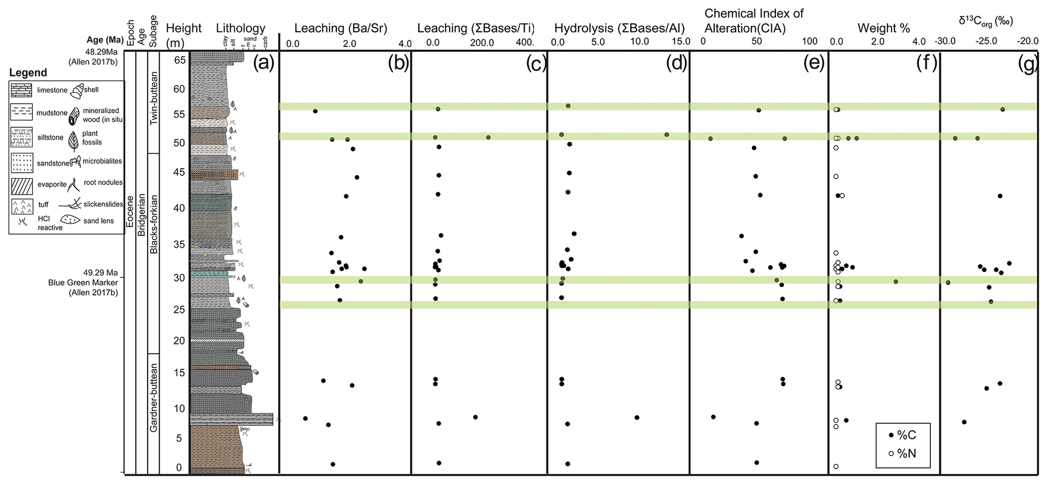
Figure 4Stratigraphy with sedimentary geochemistry. (a) Stratigraphic column at the Blue Rim escarpment of the Bridger Formation. Geochemistry including (b) leaching calculated using molar ratios of , (c) leaching calculated using the ratio of the sum of bases to titanium, (d) hydrolysis calculated using the ratio of the sum of bases to aluminum, (e) the Chemical Index of Alteration to measure weathering (Eq. 1), (f) weight % C (black circles) and % N (white circles), and (g) δ13Corg values. Light green transparent areas show stratigraphic levels containing plant fossils.
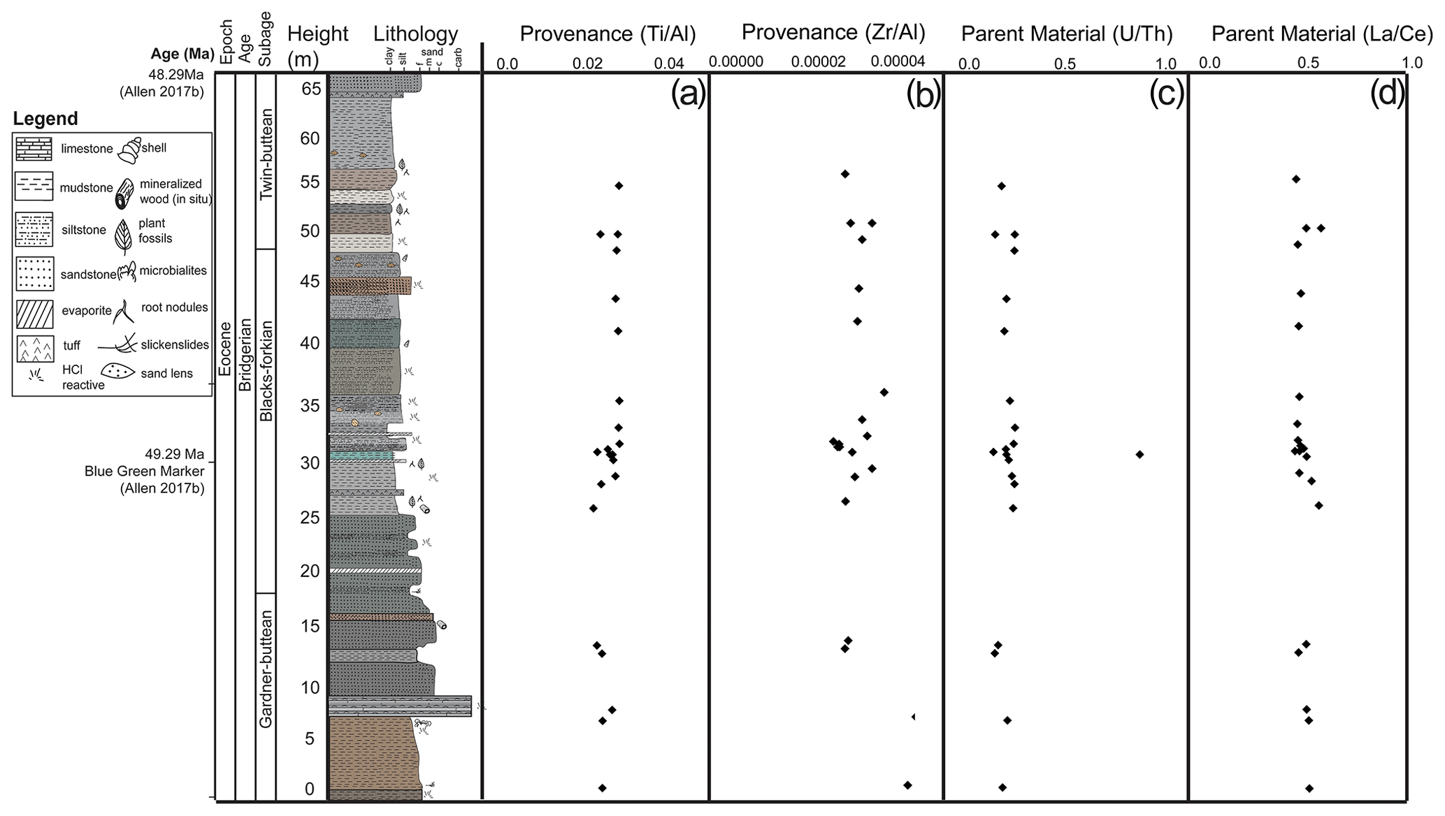
Figure 5Stratigraphy with parent material and provenance proxies. (a) Provenance using molar ratios of , (b) provenance using molar ratios of , (c) parent material using molar ratios of , and (d) parent material using molar ratios of .
3.2.4 Bulk geochemistry
Approximately 10 g aliquots of crushed paleosols, mudstone, and siltstone were measured and sent to ALS Laboratories in Vancouver, British Columbia, Canada, for bulk elemental analysis. At ALS, samples were digested with perchloric (HClO4), hydrofluoric (HF), nitric (HNO3), and hydrochloric (HCl) acids, and concentrations were determined by inductively coupled plasma (ICP) optical emission spectrometry and ICP mass spectrometry. The ICP-OES and ICP-MS were calibrated using internal standards, with major element precision better than 0.2 wt %, and error was calculated based on the maximum error of duplicates and standard tolerance. Additional information regarding the methodology is proprietary and can be sought from ALS Laboratories directly. Elements measured included aluminum (Al), arsenic (As), barium (Ba), calcium (Ca), iron (Fe), potassium (K), lanthanum (La), magnesium (Mg), sodium (Na), sulfur (S), titanium (Ti) (wt %), silver (Ag), beryllium (Be), bismuth (Bi), cadmium (Cd), cerium (Ce), cobalt (Co), chromium (Cr), cesium (Cs), copper (Cu), gallium (Ga), germanium (Ge), hafnium (Hf), indium (In), manganese (Mn), molybdenum (Mo), niobium (Nb), phosphorus (P), lead (Pb), rubidium (Rb), rhenium (Re), antimony (Sb), scandium (Sc), selenium (Se), strontium (Sr), tantalum (Ta), tellurium (Te), thorium (Th), thallium (Tl), uranium (U), vanadium (V), tungsten (W), yttrium (Y), zinc (Zn), and zirconium (Zr) (weight ppm).

Figure 6Stratigraphic column with climate proxies. (a) Reconstructed mean annual precipitation (mm yr−1) and (b) mean annual air temperature (∘C). The boxes are ranges reconstructed for physiognomic proxies, and the circles are values reconstructed using paleosols. The lines for both are established errors for the proxies used based on the initial proxy calibrations. Errors were calculated for each estimate, and the error bars span the total range of calculated error. More information on error can be found within these proxy calibrations (e.g., Wilf, 2000; Sheldon et al., 2002; Spicer et al., 2009; Gallagher and Sheldon, 2013).
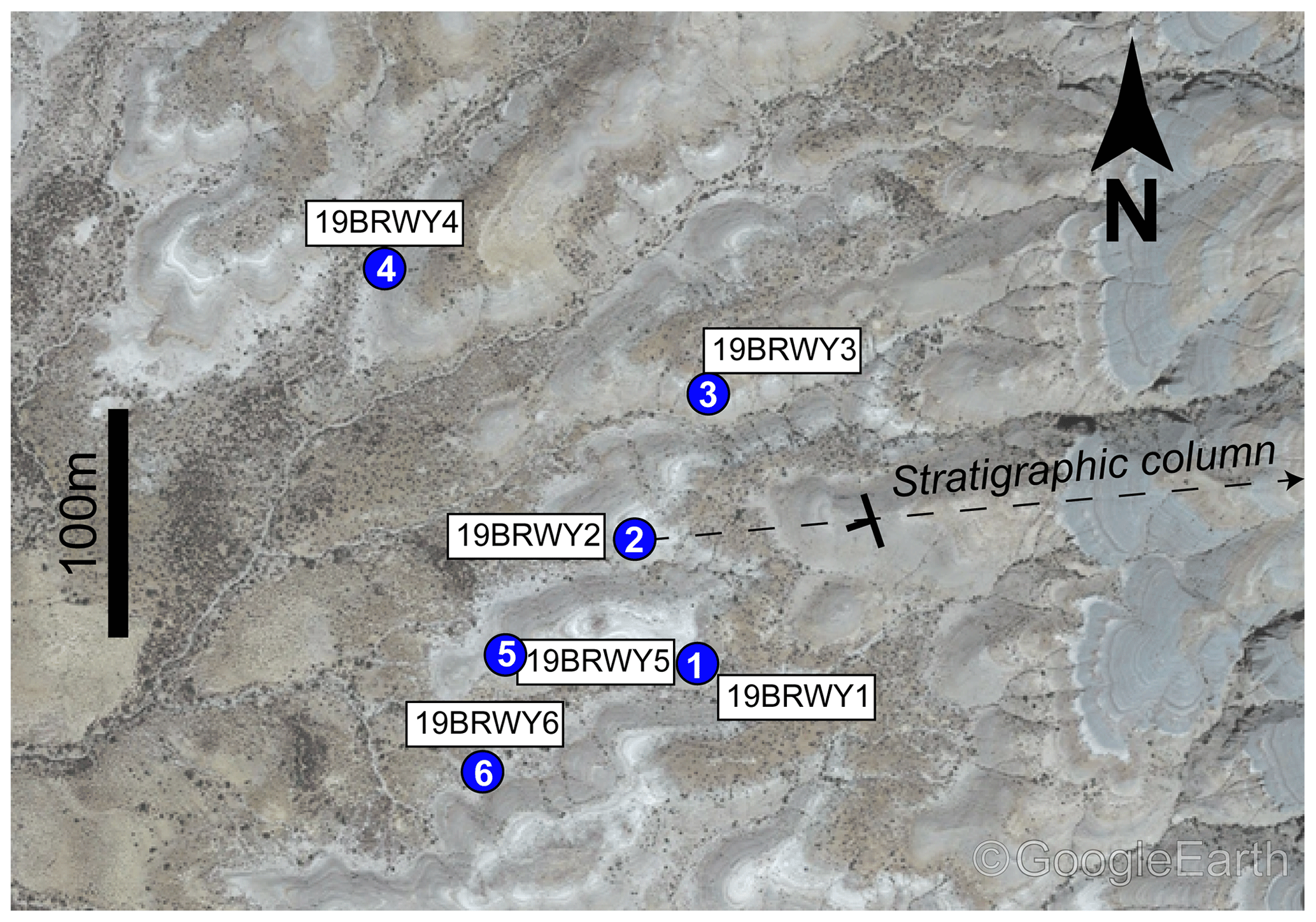
Figure 7Lateral extent of paleosols. Included are paleosols 19BRWY1-6 atop an image of the Blue Rim escarpment topography with a 100 m scale bar. Paleosol numbers are noted in white text on blue circles. Image taken in Google Earth V 9.123.0.2 (July 2019) in Wyoming, USA; 41∘48′02′′ N, 109∘35′36′′ W; eye altitude 2625 m. © Google Earth.
3.3 Paleoclimatic and paleoenvironmental calculations
3.3.1 Weathering indices and leaching
Weathering was quantified using the Chemical Index of Alteration of B horizons (CIA; Eq. 1; Nesbitt and Young, 1982), a feldspar weathering index based on the discrepancy in ion mobility during weathering.
To test for alteration and expected pedogenic elemental trends, changes in individual element mobility and strain were explored using mass balance (Eqs. 2–3; Chadwick et al., 1990), where ε represents the strain on an immobile element like Ti or Zr and τ represents the relative gain or loss of a mobile element relative to the paleosol's parent material. Average values of 2.7 and 1.5 g cm−3 were used for reworked ash and soil density, respectively (e.g., Sheldon and Tabor, 2009).
The paleosol weathering index (PWI; Eq. 4; Gallagher and Sheldon, 2013), which is based on differential bond strengths in cation oxides, provided additional means for examining weathering. Molar concentrations are used to make calculations in Eqs. (1)–(4) rather than elemental concentrations.
We used several geochemical proxies to examine intensity of leaching, including the ratio of barium to strontium (), which is higher with more leaching and lower with less leaching (Sheldon, 2006; Retallack, 2001) due to differential solubility; Sr is more soluble than Ba (Vinogradov, 1959). The ratio of the sum of base cations to titanium is another metric for leaching under the assumption that titanium is immobile, while other bases are mobile (Sheldon and Tabor, 2009). The ratio of the sum of base cations to aluminum has been used as a metric for hydrolysis (Retallack, 1999; Bestland, 2000; Sayyed and Hundekari, 2006).
3.3.2 Provenance and parent material
The molar ratios of titanium to aluminum () and zirconium to aluminum () were used to screen for consistency in sediment source in soils; direction of change in ratios is related to differences in chemical weathering, while ratios are related to changes in physical weathering (Sheldon and Tabor, 2009). The molar ratios of uranium to thorium () and lanthanum to cerium () were used to trace potential changes in parent material composition through the stratigraphic unit, where constant down-profile and ratios reflect a single-parent source (Sheldon, 2006; Sheldon and Tabor, 2009). Absolute parent material values for each of these ratios are not well calibrated, but direction of change observed at any site indicates a change in parent material. The ratio is redox-sensitive, so ratios are used as a comparative point in the case of highly reduced environments, resulting in skewed ratios.
The molar ratios of titanium to aluminum () and zirconium to aluminum () were used to screen for consistency in sediment source in soils; direction of change in ratios is related to differences in chemical weathering, while ratios are related to changes in physical weathering (Sheldon and Tabor, 2009). The molar ratios of uranium to thorium (), and lanthanum to cerium () were used to trace potential changes in parent material composition through the stratigraphic unit, where constant down-profile and ratios reflect a single-parent source (Sheldon, 2006; Sheldon and Tabor, 2009). Absolute parent material values for each of these ratios are not well calibrated, but direction of change observed at any site indicates a change in parent material. is redox-sensitive, so ratios are used as a comparative point in the case of highly reduced environments.
3.3.3 Paleoclimate reconstructions using foliar assemblages
Before and up to 2017, co-author SAE surveyed and described 69 leaf morphotypes collected from multiple quarries at Blue Rim. As per Allen's (2017b) dissertation, two techniques were used to reconstruct precipitation from foliar assemblages: the univariate approach of leaf area analysis (LAA; Wilf et al., 1998) and a multivariate approach with the Climate Leaf Analysis Multivariate Program (CLAMP; Wolfe, 1993). LAA is based on the correlation between mean leaf area and annual precipitation, related to transpiration. Leaves with higher surface-area-to-volume ratios transpire more during gas exchange; these larger leaves are typically found in wet areas (Wilf et al., 1998). Leaves in drier climates have smaller leaf-area-to-volume ratios, as they do not have as much plant-available water accessible to transpire (Wilf et al., 1998). CLAMP uses 31 morphological characters on at least 20 species of woody dicots from any given site to reconstruct 11 aspects of climate, including mean annual precipitation and mean annual temperature (MAT, comparable to mean annual air temperature – MAAT – discussed in this study; Wolfe, 1993; Spicer et al., 2009). This method is premised on the relationship between these morphological characteristics in modern flora and corresponding climate parameters.
Physiognomic techniques including CLAMP and leaf margin analysis (LMA; Wilf, 1997) were used to calculate mean annual air temperature. LMA uses the correlation between MAAT and the proportion of untoothed to total (untoothed + toothed) species in a local flora (Wolfe, 1979; Wilf, 1997; Wing and Greenwood, 1993; Peppe et al., 2011). See Allen (2017b) for additional reconstruction details based on floral assemblages.
3.3.4 Paleoclimate and paleoenvironmental reconstructions using organic and inorganic geochemistry
Mean annual precipitation was reconstructed using the Chemical Index of Alteration minus potassium (CIA-K; Eqs. 5, 6; Sheldon et al., 2002; error ± 182 mm yr−1), modified from CIA to control for potassium metasomatism in paleosols (Maynard, 1992; Ennis et al., 2000; Sheldon et al., 2002). Mean annual air temperature was calculated using PWI (Eq. 7; error of ± 2.1 ∘C; Gallagher and Sheldon, 2013). We applied the empirical relationship between δ13Cplant and δ13Catm values found by Arens et al. (2000; Eq. 8; R2 = 0.34, p<0.001) and used δ13Cplant values of all individual fossils to reconstruct generalized, non-taxon-specific δ13Catm values. We compared this reconstructed value based on a generalized equation with reconstructed values based on species-specific carbon isotope discrimination values (as measured in Cornwell et al., 2018) using fossil Lygodium and Populus to reconstruct δ13Catm values based on taxon-specific parameters (e.g., Stein et al., 2019, 2021).
Holdridge life zones are ecoregions classified by water availability and temperature that can be further subdivided into successional stages reflecting land use, disturbance history, latitude, altitude (Holdridge, 1967; Lugo et al., 1999). The parameters for each life zone are calculated based on potential evapotranspiration and humidity provinces (Holdridge, 1967; see Appendix D). Similar metrics that use evapotranspiration and precipitation to quantify ecosystems into “floral humidity provinces” based on paleosol measurements have been established more recently by Gulbranson et al. (2011; see Appendix D). See the Supplement for the methodology used to determine Holdridge life zones and floral humidity provinces for paleosols (this study) and previously published floras (Leopold and MacGinitie, 1972; Roehler, 1993; Wing et al., 2005; Smith et al., 2008; Wing and Currano, 2013; Allen, 2017a, b).
4.1 Geochronology
Single-crystal sanidine 40Ar 39Ar analyses of four sampled beds yielded ages for the middle and top of the Blue Rim escarpment that are broadly consistent with deposition during the early Eocene (Fig. 1; Tables 1, S2). Two samples (BR-3 and BR-4) of a horizon containing pumice clasts and biotite grains taken from the base and middle of the blue–green marker bed yielded similar coherent young populations of Eocene apparent ages (Figs. 4a, 8a), which are mixed with a subsidiary population of older, presumably detrital or xenocrystic grains (Fig. 8b). Sample BR-3 was collected at the base of the main blue–green marker layer just above the UF 15761S plant quarry (elevation 2053 m; Allen, 2017b), whereas sample BR-4 was collected from the lower part of the blue–green layer in the 2014/UF 19297 stratigraphic section at 2056 m (Allen, 2017b). A total of 27 of 40 fusions of sanidine from these beds form a coherent population that yields a weighted mean age of 49.29 ± 0.18 Ma (MSWD = 1.08; Table 1), which we interpret to reflect the best estimate of the age of deposition. This age is consistent with the Blue Rim being coeval with Bridger A/1b (Fig. 1).
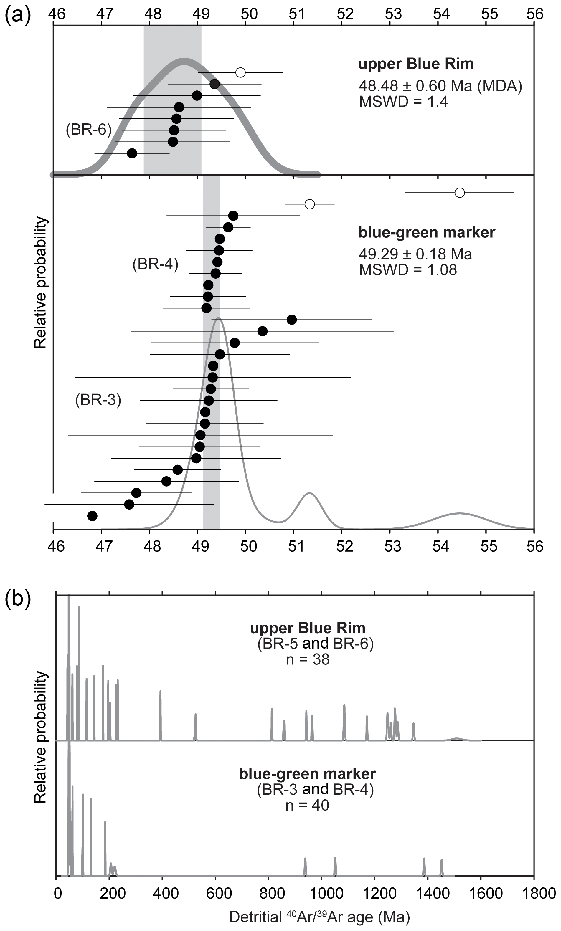
Figure 840Ar 39Ar geochronology: (a) relative probability plots of Eocene-aged sanidine from the volcaniclastic–lacustrine blue–green marker and an overlying pumice-bearing volcaniclastic sandstone (sample BR-6); (b) relative probability plot of 40Ar 39Ar ages for detrital feldspar grains from the middle and upper Blue Rim, showing Phanerozoic and late Paleozoic ages characteristic of the Idaho paleoriver (see Chetel et al., 2011).
Table 1Summary of single-crystal sanidine 40Ar 39Ar analyses: Bridger Formation, Blue Rim, WY.
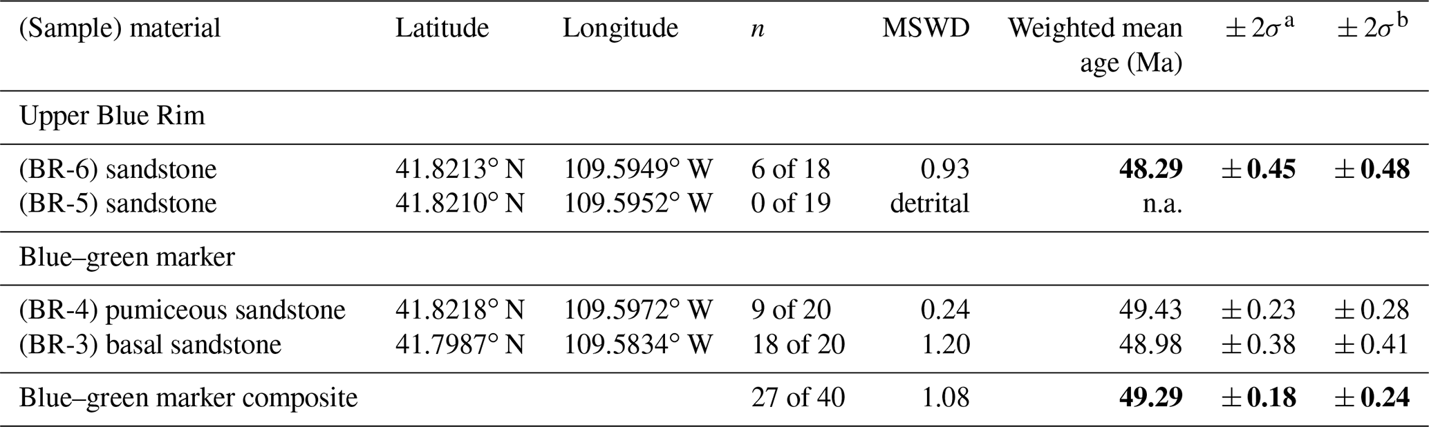
Notes: all ages are calculated relative to the 28.201 Ma age for FCs using the equations of Kuiper et al. (2008) and Renne et al. (1998) with the decay constants of Min et al. (2000) and are shown with 2σ analytical and fully propagated uncertainties, which incorporate decay constant and intercalibration uncertainties. Neutron flux monitor: FCs – Fish Canyon Tuff sanidine; see Table S2 for analytical details. Ages in bold reflect interpreted depositional ages. a Analytical uncertainty. b Fully propagated uncertainty.
Single fusions of sanidine from two sand beds (samples BR-5 and BR-6) collected near the top of the escarpment (elevation 2091 m; Allen, 2017b) yielded a greater proportion (31 of 38) of older detrital and/or xenocrystic ages than occur in samples of the blue–green marker. Nevertheless, the seven youngest grains from the uppermost sample BR-6 form a coherent population that yields a weighted mean age of 48.48 ± 0.60 Ma (MSWD = 0.60), which can be interpreted to be a maximum depositional age. This imprecise age suggests that the uppermost Blue Rim could be as old as Bridger B/B-2 or as young as Bridger D/Br-3 (Fig. 1). Altogether, new geochronology indicates that the stratigraphy between the blue–green marker bed and sand beds likely spans Bridger B, with the uppermost part of the Blue Rim escarpment being time-equivalent to Bridger C or D/3 (Figs. 4, 5, 6). This constrains the age of the lower plant horizon to be slightly older than 49.29 Ma (Allen, 2017b), whereas the upper plant horizon is likely equivalent to Bridger Br-2. Detrital or xenocrystic grains not included in weighted means discussed above yield a combination of Phanerozoic and Proterozoic apparent ages, which are consistent with detrital feldspar grains sampled from volcaniclastic strata of the Sand Butte bed of the Laney Member (Green River Formation, Smith et al., 2008; Chetel et al., 2011). The Sand Butte bed forms thick (> 40 m) deltaic foresets that prograded into and filled Lake Gosiute and parts of Lake Uintah from northwest to southeast (Surdam and Stanley, 1980; Smith et al., 2008; Chetel and Carroll, 2010). These deposits have been hypothesized to represent the inland delta or megafan of the Idaho paleoriver, which drained areas as far west as central Idaho (Chetel et al., 2011).
4.2 Paleosol descriptions
Six profiles were sampled laterally from a single paleosol at the base of the Blue Rim escarpment (located at 1 m in the stratigraphic column; Figs. 4–7). Paleosol profiles (Figs. 7, S1) typically consisted of a silty and/or sandy brown to yellow A horizon over a parent material C horizon of green–grey silty mudstone from ∼ 20 to 112 cm below the surface. Paleosol no. 1 was missing a B horizon due to erosion, while paleosol no. 4 was missing an A horizon, likely truncated during burial. Typically, each profile was lighter colored in upper horizons and darker in lower B and C horizons. In the paleosol profiles sampled, every A horizon but one, and several upper B horizons, had root traces, kerogenized roots, and/or rhizoliths. We observed drab-haloed roots in paleosols no. 1 and 4. Paleosol no. 2 had vertical burrows of up to 1 cm diameter and ∼ 3 cm length, and paleosol no. 1 had visible peds (Table S1; Fig. 3a). These soils were well-developed Inceptisols based on features, textures, and extrapolation from the local flora (Figs. 2a, S1, S5; Table S1).
4.3 Paleosol geochemistry
On average, the lateral extent of the paleosol found at the base of the Blue Rim stratigraphic section had A-horizon CIA-K values of 50–59 with a maximum of ∼ 60 in B and C horizons (consistent with expectations for CIA-K values based on past work; Sheldon et al., 2002; Sheldon and Tabor, 2009; Fig. S1b). ratios were constant throughout, ranging from 0.040 to 0.045, which is typical of values of mudstones and sandstone parented materials (Sheldon and Tabor, 2009) like those seen in sediments throughout the Blue Rim escarpment (Fig. S1c; Table S2).
Tau (used to measure mobile element transport) was calculated for soil profiles following Chadwick et al. (1990; Eqs. 2 and 3) and is displayed in Supplement Fig. S2a–f. Overall, tau values for K, Mg, and Na all ranged from 0.0 to −0.5, and tau values for Ca ranged from 0.0 to −1.0, except in paleosol no. 2 (which was extremely high in Ca), as is typical for Inceptisols. Tau values for Rb and Fe were generally also between 0.0 and −0.5, though this was less consistent between profiles. To note is that paleosol no. 1 (19BRWY1; Fig. 7) was excluded for paleoclimate reconstructions due to the lack of the presence of the B horizon (we identified this soil as an Entisol, which cannot be used for climate reconstructions; see Fig. 7 for location). Paleosol no. 2 (19BRWY2) was also excluded for climate reconstructions due to the high % Ca, which is likely of carbonate origin as this site was reactive to HCl. Likewise, the CIA-K values for 19BRWY1 and 19BRWY2 B-horizon specimens were not reasonably different than the parent material, indicating they were not in equilibrium with the environment (e.g., Sheldon and Tabor, 2009). Based on both field taxonomy and these geochemical results (see the Supplement, Table S3), paleosols no. 3–no. 6 are identified as Inceptisols (Soil Survey Staff, 2014).
4.4 Sedimentary geochemistry
All Blue Rim escarpment geochemical data have been published at the Mendeley Data Repository (https://data.mendeley.com/datasets/z6twpstz4r, last access: 24 November 2021). With a few individual outlier analyses, proxies for leaching intensity ( and sum ; Fig. 4b, c), hydrolysis (sum ; Fig. 4d), and measurements of weathering (CIA; Fig. 4e) are consistent throughout the section. Proxies for provenance also remained nearly constant (Fig. 5a, b) as did proxies for parent material (Fig. 5c, d). Organic carbon wt % was high in the same locations throughout the section as CIA, and % N was low throughout the section. δ13Corg values were the most depleted in the sections with the highest % C and % N.
4.5 Flora
The identifiable fossils from the 2019 field excursion sampled specifically for organic isotope analyses included multiple compression fossils of Lygodium kaulfussi (climbing fern, family Lygodiaceae; Manchester and Zavada, 1987), as well as one specimen of Asplenium sp. (fern, family Aspleniaceae; as described in Allen, 2017b), an example of cf. Populus cinnamomoides (poplar, family Salicaceae; Manchester et al., 2006), one specimen assigned to cf. Cedrela, (undefined species; mahogany, family Meliaceae; Fig. S5), several dense leaf mats, and assorted twig and branchlet fossils. These specimens were collected from the same strata as the lower horizon (e.g., UF 15761N, Allen, 2017b) located 26 m on the stratigraphic column included in this study (Figs. 3–5). There were also fragments of several unidentified monocots preserved, though no isotope analyses were run on these fossils.
4.6 Climate
Mean annual precipitation (MAP) values reconstructed using CIA without potash (CIA-K) on paleosol B horizons (Eq. 6) ranged from 608–1167 mm yr−1, with an average of 845 mm yr−1 (± 181 mm yr−1; n=6) (Eq. 6; Figs. 6, S6). The lowest estimated MAP value (288 mm yr−1) was excluded due to high % Ca (10.25 %) in the B horizon of paleosol 2, skewing CIA-K calculations by artificially minimizing the ratio of Al to other metals in the calculation (see Dzombak et al., 2021). Mean annual air temperature values (MAAT) reconstructed using PWI on paleosol B horizons (Eq. 7; standard error of ± 2.1 ∘C) ranged from 10.4 to 12.0 ∘C (± 0.7 ∘C standard deviation of all values from the same paleosol, or temperature reproducibility), with an average of 11.0 ∘C (n=6 profiles). Temperature reproducibility from these paleosols falls within the standard error of the paleothermometer model.
A wide range of δ13Catm values were reconstructed from δ13Cleaf from the 34 individual leaf fossils (2019 collection) using a generalized relationship (Arens et al., 2000). Reconstructions using the generalized Arens et al. (2000) model were done on all 34 individual fossil leaves, even though many of these were unidentified. Additional species-specific tests were done on all samples of Lygodium, cf. Cedrela, and Populus fossils using isotope discrimination values from extant plants of these genera. A total of 38 % (n=13) of the 34 δ13Catm values reconstructed using the generalized Arens et al. (2000) model suggested a δ13Catm value between −5.32 ‰ and −5.82 ‰; 56 % of these reconstructed values were between −5.0 ‰ and −6.0 ‰ (n=19; Eq. 8; Fig. 9). One limitation on this reconstruction is that it does not account for species-specific isotope discrimination behavior that varies taxonomically (Beerling and Royer, 2002; Stein et al., 2019; Sheldon et al., 2020). Values on the fringes (44 %) may be extreme after having experienced diagenesis of certain compounds while others were left behind, skewing the isotopic values to be representative of the compounds and not the bulk tissue (Beerling and Royer, 2002; Tu et al., 2004). Using identified Lygodium, cf. Cedrela, and Populus fossils (n=8 total), we applied the taxon-specific isotope discrimination principle and reconstructed an average value of −4.40 ‰ (minimum value of −5.23 ‰ and maximum value of −3.83 ‰). These reconstructions were based on isotope discrimination values of 19.99 ‰ for Lygodium and 20.05 ‰ for Populus (as reported in modern isotope analyses by Cornwell et al., 2018).
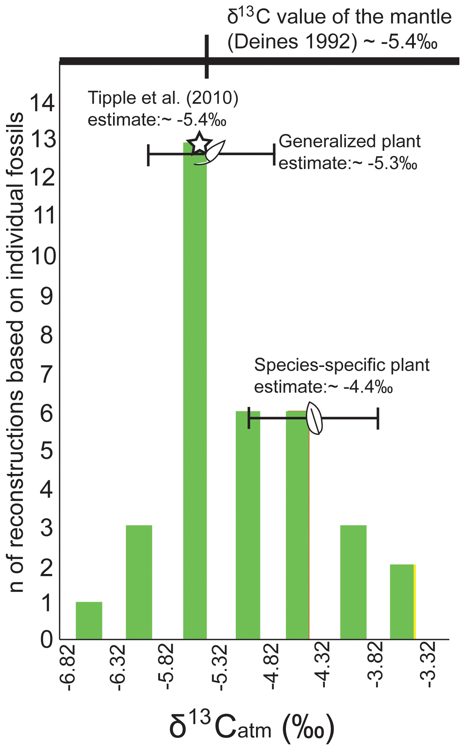
Figure 9δ13Catm as reconstructed from δ13Cleaf of the Blue Rim fossil flora. Reconstructions utilized the generalized relationship between δ13Catm and δ13Cplant (Arens et al., 2000; n=34; Eq. 8). The species-specific mean and standard deviation are shown (based on Lygodium and Populus fossils, n=8), as are the generalized plant mean and standard deviation. The Tipple et al. (2010) foraminiferal reconstruction is denoted with a star, and the δ13C value of the mantle is shown above (Deines, 1992).
5.1 Geochronology
The new 40Ar 39Ar dates presented here for the blue–green marker bed and sand beds above the floral quarries suggest that the Blue Rim section likely spans ca. 49.5 to 48.5 Ma, making it slightly younger than the EECO. Assuming constant sedimentation rates based on a linear interpolation between ages of 1 m per ∼ 23 kyr (or ∼ 44 µm yr−1, which is slightly slower than accumulation rates of 65 µm yr−1 in the Laney Member below; e.g., M. E. Smith et al., 2010), the newly described paleosols are roughly 684 300 years older than the blue–green marker bed, or 49.97 Ma. The Wilkins Peak Member and part of the Laney Member of the Green River Formation underlie the Blue Rim strata; thus, the approximate age for the paleosols based on a constant sedimentation rate is consistent with Blue Rim being younger than ∼ 50 Ma, when the Wilkins Peak Member transitioned to the Laney Member (Smith et al., 2015; see Fig. 1).
5.2 Stratigraphy, provenance, and weathering
Detrital feldspar geochronology and geochemistry strongly suggest that provenance remained constant throughout accumulation of the stratigraphic section, which can be interpreted to mean that the material did not systemically change across deposition, and geochemical proxies used to reconstruct climate are not affected by provenance shifts. A sudden 6 ‰ decrease in δ18O was previously observed in micritic lacustrine carbonates within sections of the Green River Formation, and it was hypothesized that this could be due to a sudden change in river capture to include a river with isotopically depleted waters from different headwaters (e.g., Norris et al., 1996, 2000; Doebbert et al., 2010). With new river catchments, there is a potential change in sedimentological inputs that could overwrite climate signals, so these geochemical proxies provide assurance that the climate interpretations based on geochemical proxies are not actually changes in allochthonous materials. Assumptions about provenance were supported by parent material data, which showed that all sources were primarily sedimentary. The consistent , , and ratios correspond to constant parent material throughout the 1-million-year section covered by the Blue Rim stratigraphic column, demonstrating that basin-scale hydrology was likely not reorganized during this time. The one exception to constant parent material and provenance ratios is the anomalously high ratio in the blue–green marker bed (0.87). This proxy is redox-sensitive, so this anomalously high ratio is due to the preferential redistribution and accumulation of U in this section, as Th is insoluble and immobile (Pett-Ridge et al., 2007; Sheldon and Tabor, 2009), which is intuitive with the blue–green marker color. Weathering and leaching were highest in the sections where there was high carbon content; this correlation could be due to organic acids produced by plants in the ecosystem (as represented by % C present) that contribute to chemical weathering or differences in taphonomic histories of samples. More compound-specific analyses of organic compounds would be needed to determine if and how plant influence is contributing to weathering in high % C sections (Fig. S4; R2=0.20; p-value = 0.01; Ong et al., 1970; Berner, 1992).
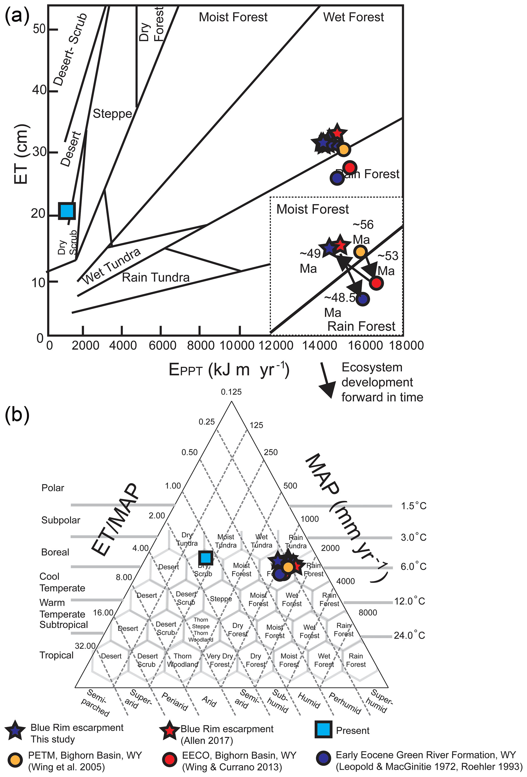
Figure 10Ecosystem-level characterization of the Blue Rim escarpment and other Cenozoic Wyoming ecosystems. Paleosol-based (a) floral humidity province and (b) Holdridge life zones (Holdridge, 1967) show with blue stars. (a) Includes an inset showing climate progression over time, with (1) the PETM (Bighorn Basin, ∼ 56 Ma), (2) the EECO (Bighorn Basin, ∼ 53 Ma), (3) this site (∼ 49 Ma), and (4) the latest stage of Lake Gosiute (Green River Formation, ∼ 48.5 Ma; Smith et al., 2008). Comparative studies for this region based on nearby temperature and precipitation reconstructions are shown with yellow, red, and blue circles, while the climate of the present (as measured in Rock Springs, Wyoming, USA) is shown as light blue squares. Average values from Allen (2017b) using leaf margin analysis to reconstruct MAAT and leaf area analysis to reconstruct MAP are shown by red stars.
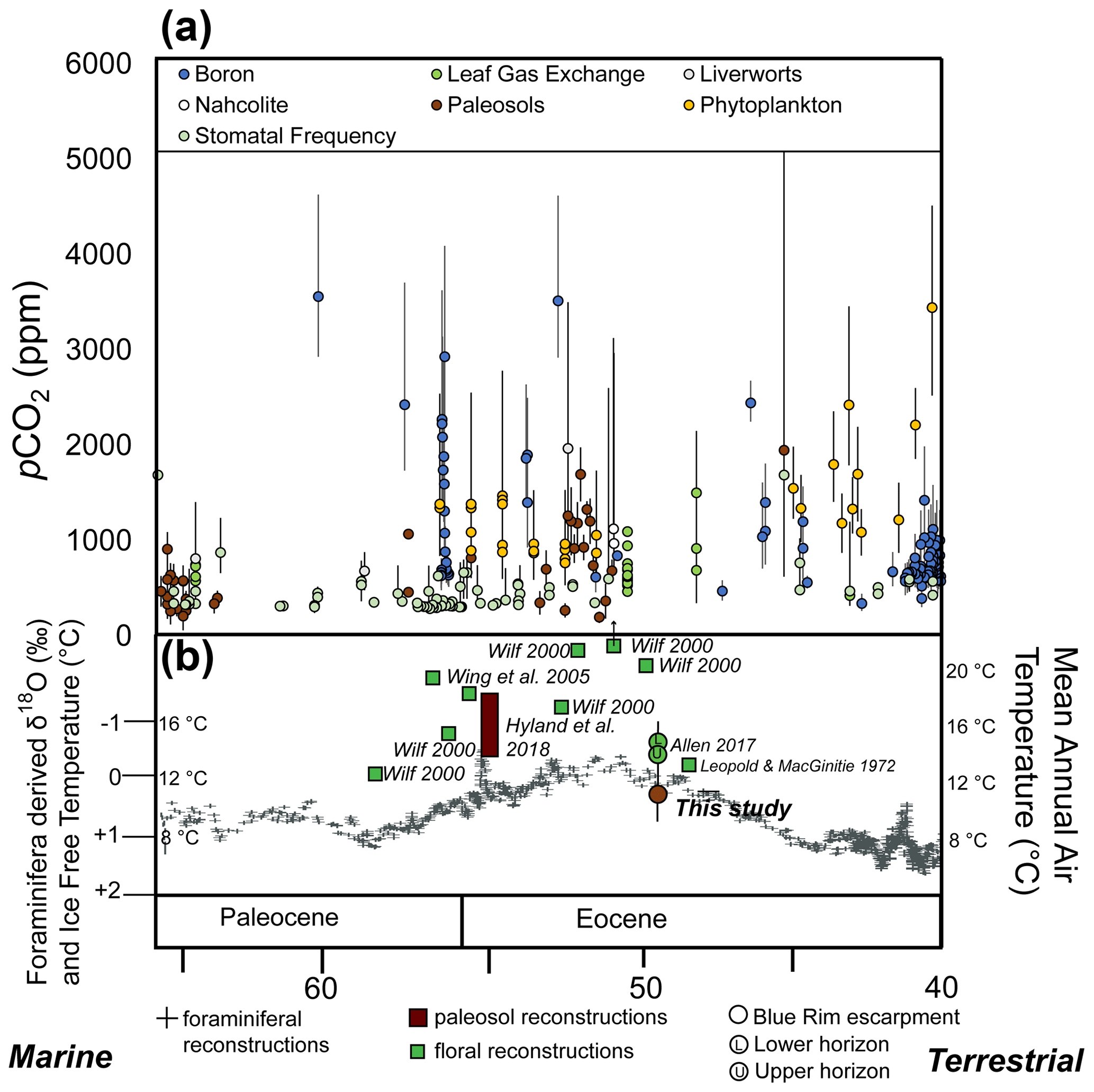
Figure 11Paleoclimate reconstructions from the Blue Rim escarpment in the context of the evolution of climate from 66 to 40 Ma. (a) pCO2 from 66 to 40 Ma based on multiple proxies compiled on paleo-CO2.org (McElwain, 1998; Ekart et al., 1999; Pearson and Palmer, 2000; Royer et al., 2001; Greenwood et al., 2003; Royer, 2003; Pagani et al., 2005; Lowenstein and Demicco, 2006; Fletcher et al., 2008; Zachos et al., 2008; Franks and Beerling, 2009; Retallack, 2009; Bijl et al., 2010; R. Y. Smith et al., 2010; Grein et al., 2011; Pagani et al., 2011; Hyland and Sheldon, 2013; Hyland et al., 2013; Huang et al., 2013; Franks et al., 2014; Maxbauer et al., 2014; Jagniecki et al., 2015; Anagnostou et al., 2016; Barclay and Wing, 2016; Liu et al., 2016; Kowalczyk et al., 2018; Witkowski et al., 2018; Zhang et al., 2018; Milligan et al., 2019; Steinthorsdottir et al., 2019; Haynes et al., 2020; Henehan et al., 2019, 2020). (b) Marine δ18O and ice-free temperature reconstructions based on foraminiferal data (Zachos et al., 2008) and mean annual air temperatures reconstructed from physiognomic (green) and paleosol (brown) proxies in the Paleocene and Eocene. Error bars are from the paleo-CO2.org site and associated citations; how they were calculated can be found in these sources.
5.3 Global and regional climate
Generally, the early Eocene of North America had widespread wet forests comparable to modern temperate and subtropical forests due to globally warmer, wetter conditions (Leopold and MacGinitie, 1972; Wing and Greenwood, 1993; Greenwood and Wing, 1995; Inglis et al., 2017; Murphey et al., 2017). Depending on the latitude of the site, other studies indicate slightly to moderately warmer conditions in temperature reconstructions from Blue Rim (Allen, 2017a, b). Generally, mean annual air temperatures reconstructed from other middle- to high-latitude sites between 36 and 80∘ N have ranges from 35 ∘C (36∘ N) to 8 ∘C (80∘ N; using leaf margin analyses and oxygen isotopes; Fricke and Wing, 2004).
More locally, temperature reconstructions of other Wyoming formations based on floral assemblages from earlier in the Eocene were higher than paleosol-based temperature reconstructions at Blue Rim (i.e., paleosol-based estimates were 12 ∘C, while other temperature reconstructions were higher; Wilf, 2000, Wing et al., 2005; Hyland et al., 2018; Fig. 11), though contemporaneous plant-based reconstructions were more comparable ∼ 12 ∘C (Leopold and MacGinitie, 1972; Allen 2017b; Fig. 11). Summer months were warm and winter months mild, with temperatures from 18 to 34 ∘C and 4 to 7 ∘C, respectively (based on Δ47; Kelson et al., 2017; Hyland et al., 2018).
The location of Blue Rim appears to have been a “wet forest” at the time of deposition, as calculated from temperature and precipitation estimates from paleosols and using leaf physiognomic techniques (see the Supplement for details; Fig. 10). The paleosol-based temperature and precipitation results are within the error of flora-only estimates based on contemporaneous Blue Rim reconstructions by Allen (2017b) and Wilf et al. (2000; other southwestern Wyoming localities including Little Mountain, Niland Tongue, Sourdough, Latham, Wasatch Main Body, Big Multi Quarry, and Bison Basin), and the ecosystem deposited is similar to Wing et al.'s (2005) ecosystem reconstruction of the Paleocene–Eocene thermal maximum (PETM; Bighorn Basin in north–central Wyoming; McInerney and Wing, 2011; Figs. 11, S7). Indeed, fossils collected for organic analysis at the Blue Rim escarpment included mineralized trunks as well as fern and angiosperm leaf macrofossils including Lygodium kaulfussii, Asplenium, Populus cinnamomoides, cf. Cedrela, and dense leaf mats. These collected fossils (sampled at 26 m on the stratigraphic section, housed at ESS laboratory at the University of Michigan) are taxonomically comparable to fossils found by Allen (2017b; Bridger Formation) and MacGinitie (1969; Green River Formation). The flora sampled are characteristic of a mesic, forested environment (e.g., wet forest; Hamzeh and Dayanandan, 2004; Hamzeh et al., 2006).
While the leaf physiognomic and paleosol-based estimates are modestly different, we cannot differentiate between whether there was a slight increase in both MAAT and MAP or whether climate was generally steady throughout the reconstructed portions of the sections because calculated values were within error. One possible explanation for the slight discrepancy between leaf physiognomic and soil-based temperature reconstructions at Blue Rim could be related to the soil taxonomy; the PWI tool used to reconstruct temperature was calibrated for Inceptisols, Alfisols, and Ultisols. However, none of the Inceptisols sampled to calibrate this proxy were from mean annual air temperatures > 12 ∘C (Gallagher and Sheldon, 2013). Therefore, it is possible that temperature reconstructions based on PWI for these Inceptisols are underestimates. Due to the complexities in the formation of soil related to seasonality of precipitation and temperature, seasonal bias has been found in paleosol reconstructions based on carbonates (e.g., Kelson et al., 2020), but B-horizon bulk geochemical data are in equilibrium with the environment and take so long to form that they not resolved enough to be affected by seasonality (e.g., Sheldon et al., 2002). Seasonal bias would not be seen in leaf physiognomic techniques either.
Leaf physiognomic proxies could contribute to the discrepancy as well; CLAMP has been cited as often producing overestimates of precipitation (Wilf et al., 1998; Allen, 2017b). This is exacerbated when there are fewer than 25 morphotypes available, which was the case at Blue Rim (Wolfe, 1993; Spicer et al., 2009; Allen, 2017b). CLAMP estimates may be less accurate due to the threshold number of morphotypes used at the Blue Rim escarpment (20); the number of morphotypes used for CLAMP temperature reconstructions was exactly the minimum recommended value (Allen, 2017b).
Regardless of the cause of discrepancy or if it represents modest actual change versus stasis, this study demonstrates the importance of the holistic approach that combines both types of proxies. However, based upon their close statistical agreement (Fig. 6) and implications for the overall ecosystem (Fig. 10), we interpret the overall climate as relatively steady (± 5 ∘C) on 100 000-year or longer timescales during this interval.
5.4 Maintaining warmth in the Paleogene
The maintenance of extended warmth and its relation to elevated CO2 during the early Eocene is debated (Hyland and Sheldon, 2013; Anagnostou et al., 2016; Gutjahr et al., 2017; Cramwinckel et al., 2018), which emphasizes the importance of δ13Catm values that can help to contextualize potential CO2 sources. Some scientists invoke the destabilization of deep-sea methane hydrates as the mechanism for CO2 increase (e.g., Dickens, 2011), while others pinpoint volcanic emissions (Reagan et al., 2013; Gutjahr et al., 2017; Jones et al., 2019) and reduced silica weathering (Zachos et al., 2008; Lunt et al., 2011). These mechanisms occur on very different timescales (e.g., methane has a lifetime of 12 years in the atmosphere; Schiermeier, 2020) and thus require vastly different environmental processes and landscapes. It is possible to determine changes in the source of atmospheric CO2 by examining the isotopic signature of the atmosphere; volcanic CO2 has an isotopic composition of −5.4 ‰ (Deines, 1992), while methane hydrates are far more depleted (e.g., −64.5 ‰ to −67.5 ‰ off the coast of central Oregon; Kastner et al., 1998). As mentioned above, based on the comparative Arens et al. (2000) model, δ13Cleaf values can be used to infer δ13Catm values. These values are also important parameters in models that reconstruct additional environmental variables, such as the concentration of atmospheric CO2 using paleosol carbonates (Cerling et al., 1991; Cerling, 1992) or using stomatal parameters (Franks et al., 2014). Our large sample size of distinguishable leaf fossils from a single horizon (n=34) allowed us to statistically determine the most likely δ13Catm value based on the general relationship proposed by Arens et al. (2000) to be between −5.32 ‰ and −5.82 ‰. Analyses with taxon-specific reconstructions (n=9 total specimens of these genera: Lygodium, cf. Cedrela, and Populus fossils) using extant members of these genera to determine isotope discrimination and reconstruct the atmosphere (as published in Cornwell et al., 2018) had an average value of −4.82 ‰ (± 0.92 ‰ standard deviation). Both generalized and taxon-specific reconstructions were within the error of the isotopic value of mantle CO2 (−5.4 ‰; Deines, 1992) and comparable to the value reconstructed for ∼ 49 Ma using benthic and planktonic foraminifera of −5.4 ‰ (Tipple et al., 2010). Although we cannot rule out short-term perturbations of other C pools (e.g., methane hydrates during the PETM, Foster et al., 2018; shift in carbon from the deep ocean due to changes in the carbon compensation depth; Zeebe et al., 2009; Pälike et al., 2012; Zeebe, 2012), these results support previous findings indicating a long-term volcanic source of CO2 that drove long-term warmth in the Paleogene. However, this observation is incomplete without full constraints regarding the calcite compensation depth and the distribution of carbon isotopes in carbon ocean chemistry (e.g., Komar et al., 2013), both of which are not constrained in the scope of this study. As per other studies, the early Cenozoic period of elevated rates of volcanism (locally in the Rocky Mountains; e.g., Challis volcanics; Fig. 3a; Chetel et al., 2011; globally with the North American Igneous Province; ∼ 61 to ∼ 50 Ma; e.g., Meyer et al., 2007; Storey et al., 2007) can account for this.
The age findings contained in this study constrain the time for the Blue Rim wet forests to be slightly younger than previous estimates, with the upper half of the section clearly deposited after the EECO. Based on dating and sedimentation rates, the lower part of the section could overlap with the end of the EECO, but there is an absence of observable changes in proxy records. During the EECO, the Blue Rim escarpment received between 608 and 1167 mm yr−1 of precipitation, likely related to different moisture regimes, and was a productive paratropical (non-equatorial tropical) forest. Although reconstructed temperature and precipitation values using paleosol and sedimentary geochemistry are lower than published values reconstructed from flora, the values from all the proxies fall within error of one another (see the Supplement). Furthermore, the Holdridge life zones and floral humidity provinces calculated for both leaf physiognomic-based and geochemistry-based reconstructions are comparable, pinpointing this region as a warm, wet forest at ∼ 49 Ma.
The new age constraints, evidence from leaf fossils, and inorganic and organic geochemical proxies at the Blue Rim escarpment make it possible to reconstruct the depositional environment of the central region of Lake Gosiute in an unprecedented way. The consistent , , and ratios to determine provenance and parent material throughout the Blue Rim stratigraphic column demonstrate that the hydrological and sedimentological inputs remained stable for this location throughout the ∼ 1 million years spanned by this section. The use of multiple proxies to cross-compare sites is under-utilized in paleoclimate reconstructions but allows for an improved understanding of regional and more broad-scale climate regimes. Based on ample floral and geochemical data, ∼ 49.5–48.5 million years ago – after the peak of the EECO – southwestern Wyoming was a warm, wet forest atop deltaic deposition (Fig. 3a; Chetel et al., 2011) with little to no frost and mild temperatures, in agreement with previous work based only on fossil floras (e.g., MacGinitie, 1969; Wilf, 2000) or paleosols (Hyland et al., 2018) individually.
The geochemical dataset for this paper can be found at the Mendeley Data Repository under the title “Blue Rim escarpment geochemical data”, Mendeley Data, V1: https://doi.org/10.17632/z6twpstz4r.2 (Stein and Sheldon, 2021).
The supplement related to this article is available online at: https://doi.org/10.5194/cp-17-2515-2021-supplement.
NDS and RAS conceived and designed the study. RMD and RAS collected the data in the field. MES, SEA, and BRJ contributed data. NDS and MES were responsible for funding acquisition, and RAS acquired funding for fieldwork. NDS was responsible for project administration, provision of resources, and supervision for RAS. RAS was primarily responsible for the investigation and performed many of the visualizations. RMD, MES, and SEA contributed visualizations as well. RAS and NDS were responsible for the original draft, and all authors (RMD, RAS, MES, SEA, BRJ) were responsible for review and editing.
The contact author has declared that neither they nor their co-authors have any competing interests.
Publisher's note: Copernicus Publications remains neutral with regard to jurisdictional claims in published maps and institutional affiliations.
We thank Nikolas C. Midttun for assistance measuring, creating, and sampling the stratigraphic column at the Blue Rim escarpment in June 2019. We thank Steven R. Manchester for personal communications regarding the location of floral fossil quarries at Blue Rim. We thank Selena Y. Smith for personal communications and consultation regarding fossils and for access to her camera and camera stand for fossil photographs. We acknowledge Naomi E. Levin, Christopher J. Poulsen, and Gretchen Keppel-Aleks for their feedback on this paper.
This research has been supported by the National Science Foundation (grant no. 1812949 to Nathan D. Sheldon and Michael E. Smith) and the Evolving Earth Foundation (Graduate Student Research Grant).
This paper was edited by Alberto Reyes and reviewed by Erik Gulbranson and one anonymous referee.
Allen, S. E.: Fossil palm flowers from the Eocene of the Rocky Mountain region with affinities to Phoenix L. (Arecaceae: Coryphoideae), Int. J. Plant Sci., 176, 586–596, 2015.
Allen, S. E.: Reconstructing the local vegetation and seasonality of the Lower Eocene Blue Rim site of southwestern Wyoming using fossil wood, Int. J. Plant Sci., 17, 689–714, 2017a.
Allen, S. E.: The Uppermost Lower Eocene Blue Rim Flora from the Bridger Formation of Southwestern Wyoming: Floristic Composition, Paleoclimate, and Paleoecology, Doctoral Dissertation, University of Florida, 2017b.
Allen, S. E., Stull, G. W., and Manchester, S. R.: Icacinaceae from the Eocene of western North America, Am. J. Bot., 102, 725–744, 2015.
Anagnostou, E., John, E. H., Edgar, K. M., Foster, G. L., Ridgwell, A., Inglis, G. N., Pancost, R. D., Lunt, D. J., and Pearson, P. N.: Changing atmospheric CO2 concentration was the primary driver of early Cenozoic climate, Nature, 533, 380–384, 2016.
Arens, N. C., Jahren, A. H., and Amundson, R.: Can C3 plants faithfully record the carbon isotopic composition of atmospheric carbon dioxide?, Paleobiology, 26, 137–164, 2000.
Barclay, R. S. and Wing, S. L.: Improving the Ginkgo CO2 barometer: implications for the early Cenozoic atmosphere, Earth Planet. Sc. Lett., 439, 158–171, 2016.
Beerling, D. J. and Royer, D. L.: Fossil plants as indicators of the Phanerozoic global carbon cycle, Ann. Rev. Earth Pl. Sc., 30, 527–556, 2002.
Berner, R. A.: Weathering, plants, and the long-term carbon cycle, Geochim. Cosmochim. Ac., 56, 3225–3231, 1992.
Bernstein, L., Bosch, P., Canziani, O., Chen, Z., Christ, R., and Riahi, K.: IPCC, climate change 2007, synthesis report, 2007.
Bestland, E. A.: Weathering flux and CO2 consumption determined from paleosol sequences across the Eocene–Oligocene transition, Palaeogeogr. Palaeocl., 156, 301–326, 2000.
Bijl, P. K., Houben, A. J., Schouten, S., Bohaty, S. M., Sluijs, A., Reichart, G. J., Damsté, J. S. S., and Brinkhuis, H.: Transient Middle Eocene atmospheric CO2 and temperature variations, Science, 330, 819–821, 2010.
Boutton, T. W.: Stable Carbon Isotope Ratios of Natural Materials: I. Sample Preparation and Mass Spectrometric, Carbon isotope techniques, 1, 152–155, 1991.
Brand, L. R., Goodwin, H. T., Ambrose, P. D., and Buchheim, H. P.: Taphonomy of turtles in the middle Eocene Bridger Formation, SW Wyoming, Palaeogeogr. Palaeocl., 162, 171–189, 2000.
Breedlovestrout, R. L., Evraets, B. J., and Parrish, J. T.: New Paleogene climate analysis of western Washington using physiognomic characteristics of fossil leaves, Palaeogeogr. Palaeocl., 392, 22–40, 2013.
Buchheim, H. P., Brand, L. R., and Goodwin, H. T.: Lacustrine to fluvial floodplain deposition in the Eocene Bridger Formation, Palaeogeogr. Palaeocl., 162, 191–209, 2000.
Carmichael, M. J., Inglis, G. N., Badger, M. P., Naafs, B. D. A., Behrooz, L., Remmelzwaal, S., Monteiro, F. M., Rohrssen, M., Farnsworth, A., Buss, H. L., Dickson, A. J., Valdes, P. J., Lunt, D. J., and Pancost, R. D. Hydrological and associated biogeochemical consequences of rapid global warming during the Paleocene-Eocene Thermal Maximum, Glob. Planet. Change, 157, 114–138, 2017.
Cerling, T. E., Solomon, D. K., Quade, J. A. Y., and Bowman, J. R.: On the isotopic composition of carbon in soil carbon dioxide, Geochim. Cosmochim. Ac., 55, 3403–3405, 1991.
Cerling, T. E.: Use of carbon isotopes in paleosols as an indicator of the P(CO2) of the paleoatmosphere, Global Biogeochem. Cy., 6, 307–314, 1992.
Chadwick, O. A., Brimhall, G. H., and Hendricks, D. M.: From a black to a gray box – a mass balance interpretation of pedogenesis, Geomorphology, 3, 369–390, 1990.
Cheeseman, J.: Food security in the face of salinity, drought, climate change, and population growth, in: Halophytes for food security in dry lands, Academic Press, 111–123, 2016.
Chetel, L. M. and Carroll, A. R.: Terminal infill of Eocene Lake Gosiute, Wyoming, USA, J. Sediment. Res., 80, 492–514, 2010.
Chetel, L. M., Janecke, S. U., Carroll, A. R., Beard, B. L., Johnson, C. M., and Singer, B. S.: Paleogeographic reconstruction of the Eocene Idaho River, North American Cordillera, GSA Bulletin, 123, 71–88, 2011.
Clyde, W. C., Sheldon, N. D., Koch, P. L., Gunnell, G. F., and Bartels, W. S.: Linking the Wasatchian/Bridgerian boundary to the Cenozoic Global Climate Optimum: new magnetostratigraphic and isotopic results from South Pass, Wyoming, Palaeogeogr. Palaeocl., 167, 175–199, 2001.
Coats, S., Smerdon, J. E., Cook, B. I., and Seager, R.: Are simulated megadroughts in the North American Southwest forced?, J. Clim., 28, 124–142, 2015.
Cotton, J. M., Jeffery, M. L., and Sheldon, N. D.: Climate controls on soil respired CO2 in the United States: implications for 21st century chemical weathering rates in temperate and arid ecosystems, Chem. Geol., 358, 37–45, 2013.
Cornwell, W. K., Wright, I. J., Turner, J., Maire, V., Barbour, M. M., Cernusak, L. A., Dawson, T., Ellsworth, D., Farquhar, G. D., Griffiths, H., and Keitel, C.: Climate and soils together regulate photosynthetic carbon isotope discrimination within C3 plants worldwide, Glob. Ecol. Biogeogr., 27, 1056–1067, 2018.
Cramwinckel, M. J., Huber, M., Kocken, I. J., Agnini, C., Bijl, P. K., Bohaty, S. M., Frieling, J., Goldner, A., Hilgen, F. J., Kip, E. L., Peterse, F., and Sluijs, A.: Synchronous tropical and polar temperature evolution in the Eocene, Nature, 559, 382–386, 2018.
DeCelles, P. G.: Late Jurassic to Eocene evolution of the Cordilleran thrust belt and foreland basin system, western USA, Am. J. Sci., 304, 105–168, 2004.
Deines, P.: Mantle carbon: concentration, mode of occurrence, and isotopic composition, in: Early Organic Evolution, Springer, Berlin, Heidelberg, 133–146, 1992.
Dickinson, W. R., Klute, M. A., Hayes, M. J., Janecke, S. U., Lundin, E. R., McKittrick, M. A., and Olivares, M. D.: Paleogeographic and paleotectonic setting of Laramide sedimentary basins in the central Rocky Mountain region, Geol. Soc. Am. Bull., 100, 1023–1039, 1988.
Dickens, G. R.: Down the Rabbit Hole: toward appropriate discussion of methane release from gas hydrate systems during the Paleocene-Eocene thermal maximum and other past hyperthermal events, Clim. Past, 7, 831–846, https://doi.org/10.5194/cp-7-831-2011, 2011.
Dillhoff, R. M., Dillhoff, T. A., Greenwood, D. R., DeVore, M. L., and Pigg, K. B.: The Eocene Thomas Ranch flora, Allenby Formation, Princeton, British Columbia, Canada, Botany, 91, 514–529, 2013.
Doebbert, A. C., Carroll, A. R., Mulch, A., Chetel, L. M., and Chamberlain, C. P.: Geomorphic controls on lacustrine isotopic compositions: evidence from the Laney Member, Green River Formation, Wyoming, GSA Bull., 122, 236–252, 2010.
Dzombak, R. M., Midttun, Nikolas C., Stein, R. A., and Sheldon, N. D.: Incorporating lateral variability and extent of paleosols into proxy uncertainty, Palaeogeogr. Palaeocl., 582, 110641, https://doi.org/10.1016/j.palaeo.2021.110641, 2021.
Ekart, D. D., Cerling, T. E., Montanez, I. P., and Tabor, N. J.: A 400-million-year carbon isotope record of pedogenic carbonate: implications for paleoatmospheric carbon dioxide, Am. J. Sci., 299, 805–827, 1999.
Emry, R. J.: Mammals of the Bridgerian (middle Eocene) Elderberry Canyon local fauna of eastern Nevada, Geol. Soc. Am. Spec. Paper, 243, 187–210, 1990.
Ennis, D. J., Dunbar, N. W., Campbell, A. R., and Chapin, C. E.: The effects of K-metasomatism on the mineralogy and geochemistry of silicic ignimbrites near Socorro, New Mexico, Chem. Geol., 167, 285–312, 2000.
Fletcher, B. J., Brentnall, S. J., Anderson, C. W., Berner, R. A., and Beerling, D. J.: Atmospheric carbon dioxide linked with Mesozoic and early Cenozoic climate change, Nat. Geosci., 1, 43–48, 2008.
Foster, G. L., Hull, P., Lunt, D. J., and Zachos, J. C.: Placing our current “hyperthermal” in the context of rapid climate change in our geological past, Philoso. T. R. Soc. A, 376, 20170086, https://doi.org/10.1098/rsta.2017.0086, 2018.
Franks, P. J. and Beerling, D. J.: CO2-forced evolution of plant gas exchange capacity and water-use efficiency over the Phanerozoic, Geobiology, 7, 227–236, 2009.
Franks, P. J., Royer, D. L., Beerling, D. J., Van de Water, P. K., Cantrill, D. J., Barbour, M. M., and Berry, J. A.: New constraints on atmospheric CO2 concentration for the Phanerozoic, Geophys. Res. Lett., 41, 4685–4694, 2014.
Fricke, H. C. and Wing, S. L.: Oxygen isotope and paleobotanical estimates of temperature and δ18O–latitude gradients over North America during the early Eocene, Am. J. Sci., 304, 612–635, 2004.
Gallagher, T. M. and Sheldon, N. D.: A new paleothermometer for forest paleosols and its implications for Cenozoic climate, Geology, 41, 647–650, 2013.
Gingerich, P. D.: Mammalian responses to climate change at the Paleocene-Eocene boundary: Polecat Bench record in the northern Bighorn Basin, Wyoming, in: Causes and Consequences of Globally Warm Climates in the Early Paleogene, edited by: Wing, S. L., Gingerich, P. D., Schmitz, B., and Thomas, E., Geol. Soc. Am. Sp. Paper, 369, 463–478, 2003.
Greenwood, D. R. and Wing, S. L.: Eocene continental climates and latitudinal temperature gradients, Geology, 23, 1044–1048, 1995.
Greenwood, D. R., Scarr, M. J., and Christophel, D. C.: Leaf stomatal frequency in the Australian tropical rainforest tree Neolitsea dealbata (Lauraceae) as a proxy measure of atmospheric pCO2, Palaeogeogr. Palaeocl., 196, 375–393, 2003.
Greenwood, D. R., Pigg, K. B., Basinger, J. F., and DeVore, M. L.: A review of paleobotanical studies of the Early Eocene Okanagan (Okanogan) Highlands floras of British Columbia, Canada and Washington, USA, Can. J. Earth Sci., 53, 548–564, https://doi.org/10.1139/cjes-2015-0177, 2016.
Grein, M., Konrad, W., Wilde, V., Utescher, T., and Roth-Nebelsick, A.: Reconstruction of atmospheric CO2 during the early middle Eocene by application of a gas exchange model to fossil plants from the Messel Formation, Germany, Palaeogeogr. Palaeocl., 309, 383–391, 2011.
Gulbranson, E. L., Montanez, I. P., and Tabor, N. J.: A proxy for humidity and floral province from paleosols, J. Geol., 119, 559–573, 2011.
Guiot, J., Wu, H. B., Garreta, V., Hatté, C., and Magny, M.: A few prospective ideas on climate reconstruction: from a statistical single proxy approach towards a multi-proxy and dynamical approach, Clim. Past, 5, 571–583, https://doi.org/10.5194/cp-5-571-2009, 2009.
Gutjahr, M., Ridgwell, A., Sexton, P. F., Anagnostou, E., Pearson, P. N., Pälike, H., Morris, R. D., Thomas, E., and Foster, G. L.: Very large release of mostly volcanic carbon during the Palaeocene–Eocene Thermal Maximum, Nature, 548, 573–577, 2017.
Hamzeh, M., and Dayanandan, S.: Phylogeny of Populus (Salicaceae) based on nucleotide sequences of chloroplast TRNT-TRNF region and nuclear rDNA, Am. J. Bot., 91, 1398–1408, 2004.
Hamzeh, M., Périnet, P., and Dayanandan, S.: Genetic Relationships among species of Populus (Salicaceae) based on nuclear genomic data, J. Torr. Bot. Soc., 133, 519–527, 2006.
Haynes, S. J., MacLeod, K. G., Ladant, J. B., Guchte, A. V., Rostami, M. A., Poulsen, C. J., and Martin, E. E.: Constraining sources and relative flow rates of bottom waters in the Late Cretaceous Pacific Ocean, Geology, 48, 509–513, 2020.
Henehan, M. J., Ridgwell, A., Thomas, E., Zhang, S., Alegret, L., Schmidt, D. N., Rae, J. W., Witts, J. D., Landman, N. H., Green, S. E., and Huber, B. T.: Rapid ocean acidification and protracted Earth system recovery followed the end-Cretaceous Chicxulub impact, P. Natl. Acad. Sci., 116, 22500–22504, 2019.
Henehan, M., Edgar, K., Foster, G., Oenman, D., Hull, P., Greenop, R., Anagnostou, E., and Pearson, P.: Revisiting the Middle Eocene Climatic Optimum “Carbon Cycle Conundrum” with new estimates of atmospheric pCO2 from boron isotopes, Paleoceanogr. Paleocl., 35, e2019PA003713, https://doi.org/10.1029/2019PA003713, 2020.
Henry, C. D., Hinz, N. H., Faulds, J. E., Colgan, J. P., John, D. A., Brooks, E. R., and Castor, S. B.: Eocene–Early Miocene paleotopography of the Sierra Nevada–Great Basin–Nevadaplano based on widespread ash-flow tuffs and paleovalleys, Geosphere, 8, 1–27, 2012.
Holdridge, L. R.: Life Zone Ecology, Tropical Science Center, San Jose, Costa Rica, 1–206, 1967.
Huang, C., Retallack, G. J., Wang, C., and Huang, Q.: Paleoatmospheric pCO2 fluctuations across the Cretaceous–Tertiary boundary recorded from paleosol carbonates in NE China, Palaeogeogr. Palaeocl., 385, 95–105, 2013.
Hyland, E. G. and Sheldon, N. D.: Coupled CO2-climate response during the early Eocene climatic optimum, Palaeogeogr. Palaeocl., 369, 125–135, 2013.
Hyland, E., Sheldon, N. D., and Fan, M.: Terrestrial paleoenvironmental reconstructions indicate transient peak warming during the early Eocene climatic optimum, GSA Bull., 125, 1338–1348, 2013.
Hyland, E. G., Huntington, K. W., Sheldon, N. D., and Reichgelt, T.: Temperature seasonality in the North American continental interior during the Early Eocene Climatic Optimum, Clim. Past, 14, 1391–1404, https://doi.org/10.5194/cp-14-1391-2018, 2018.
Inglis, G. N., Collinson, M. E., Riegel, W., Wilde, V., Farnsworth, A., Lunt, D. J., Valdes, P., Robson, B. E., Scott, A. C., Lenz, O. K., Naafs, B. D. A., and Pancost, R. D.: Mid-latitude continental temperatures through the early Eocene in western Europe, Earth Planet. Sc. Lett., 460, 86–96, 2017.
Jagniecki, E. A., Lowenstein, T. K., Jenkins, D. M., and Demicco, R. V.: Eocene atmospheric CO2 from the nahcolite proxy, Geology, 43, 1075–1078, 2015.
Jones, S. M., Hoggett, M., Greene, S. E., and Jones, T. D.: Large Igneous Province thermogenic greenhouse gas flux could have initiated Paleocene-Eocene Thermal Maximum climate change, Nat. Commun., 10, 1–16, 2019.
Kastner, M., Kvenvolden, K. A., and Lorenson, T. D.: Chemistry, isotopic composition, and origin of a methane-hydrogen sulfide hydrate at the Cascadia subduction zone, Earth Planet. Sc. Lett., 156, 173–183, 1998.
Keeling, C. D., MOOK, W. G., and Tans, P. P.: Recent trends in the 13C 12C ratio of atmospheric carbon dioxide, Nature, 277, 121–123, 1979.
Kelson, J. R., Huntington, K. W., Schauer, A. J., Saenger, C., and Lechler, A. R.: Toward a universal carbonate clumped isotope calibration: Diverse synthesis and preparatory methods suggest a single temperature relationship, Geochim. Cosmochim. Ac., 197, 104–131, 2017.
Kelson, J. R., Huntington, K. W., Breecker, D. O., Burgener, L. K., Gallagher, T. M., Hoke, G. D., and Petersen, S. V.: A proxy for all seasons? A synthesis of clumped isotope data from Holocene soil carbonates, Quaternary Sci. Rev., 234, 106259, https://doi.org/10.1016/j.quascirev.2020.106259, 2020.
Kistner, F. B.: Stratigraphy of the Bridger Formation in the Big Island-Blue Rim area, Sweetwater County, Wyoming, Masters' Thesis, University of Wyoming, Laramie, Wyoming, 1973.
Koenig, K. J.: Bridger Formation in the Bridger Basin, Wyoming, Overthrust Belt of Southwestern Wyoming and Adjacent Areas, 15th Annual Field Conference Guidebook, 163–168, 1960.
Komar, N., Zeebe, R. E., and Dickens, G. R.: Understanding long-term carbon cycle trends: The late Paleocene through the early Eocene, Paleoceanography, 28, 650–662, 2013.
Kowalczyk, J. B., Royer, D. L., Miller, I. M., Anderson, C. W., Beerling, D. J., Franks, P. J., Grein, M., Konrad, W., Roth-Nebelsick, A., Bowring, S. A., and Johnson, K. R.: Multiple proxy estimates of atmospheric CO2 from an early Paleocene rainforest, Paleoceanogr. Paleocl., 33, 1427–1438, 2018.
Kowalski, E. A. and Dilcher, D. L.: Warmer paleotemperatures for terrestrial ecosystems, P. Natl. Acad. Sci. USA, 100, 167–170, 2003.
Kuiper, K. F. A., Deino, F. J. K., Hilgen, W., Renne, P. R., and Wijbrans, J. R.: Synchonizing rock clocks of Earth history, Science, 320, 500–504, 2008.
Leopold, E. B. and MacGinitie, H. D.: Development and affinities of Tertiary floras in the Rocky Mountains, in: Floristics and Paleoflorists of Asia and Eastern North America, edited by: Graham, A., Elsevier Publishing Company, 147–200, 1972.
Li, B., Nychka, D. W., and Ammann, C. M.: The value of multiproxy reconstruction of past climate, J. Am. Stat. Assoc., 105, 883–895, 2010.
Liu, X. Y., Gao, Q., Han, M., and Jin, J. H.: Estimates of late middle Eocene pCO2 based on stomatal density of modern and fossil Nageia leaves, Clim. Past, 12, 241–253, https://doi.org/10.5194/cp-12-241-2016, 2016.
Looy, C., Kerp, H., Duijnstee, I., and DiMichele, B.: The late Paleozoic ecological-evolutionary laboratory, a land-plant fossil record perspective, Sediment. Record, 12, 4–18, 2014.
Lowenstein, T. K. and Demicco, R. V.: Elevated Eocene atmospheric CO2 and its subsequent decline, Science, 313, 1928–1928, 2006.
Lugo, A. E., Brown, S. L., Dodson, R., Smith, T. S., and Shugart, H. H.: The Holdridge life zones of the conterminous United States in relation to ecosystem mapping, J. Biogeogr., 26, 1025–1038, 1999.
Lunt, D. J., Ridgwell, A., Sluijs, A., Zachos, J., Hunter, S., and Haywood, A.: A model for orbital pacing of methane hydrate destabilization during the Palaeogene, Nat. Geosci., 4, 775–778, 2011.
MacGinitie, H. D.: The Eocene Green River flora of northwestern Colorado and northeastern Utah, University of California Press, Berkeley, California, USA 1969.
Manchester, S. R. and Zavada, M. S.: Lygodium foliage with intact sorophores from the Eocene of Wyoming, Bot. Gaz., 148, 392–399, 1987.
Manchester, S. R., Judd, W. S., and Handley, B.: Foliage and fruits of early poplars (Salicaceae: Populus) from the Eocene of Utah, Colorado, and Wyoming, Int. J. Plant Sci., 167, 897–908, 2006.
Matthew, W. D.: The Carnivora and Insectivora of the Bridger basin, middle Eocene, EW Wheeler, printer, Bulletin of the American Museum of Natural History, New York, NY, 1909.
Maxbauer, D. P., Royer, D. L., and LePage, B. A.: High Arctic forests during the middle Eocene supported by moderate levels of atmospheric CO2, Geology, 42, 1027–1030, 2014.
Maxbauer, D. P., Feinberg, J. M., Fox, D. L., and Clyde, W. C.: Magnetic minerals as recorders of weathering, diagenesis, and paleoclimate: A core–outcrop comparison of Paleocene – Eocene paleosols in the Bighorn Basin, WY, USA, Earth Planet. Sc. Lett., 452, 15–26, 2016.
Maynard, J. B.: Chemistry of modern soils as a guide to interpreting Precambrian paleosols, J. Geol., 100, 279–289, 1992.
McElwain, J. C.: Do fossil plants signal palaeoatmospheric carbon dioxide concentration in the geological past?, Philos. T. R. Soc. Lond. Ser. B, 353, 83–96, 1998.
McInerney, F. A. and Wing, S. L.: The Paleocene-Eocene Thermal Maximum: A perturbation of carbon cycle, climate, and biosphere with implications for the future, Annu. Rev. Earth Pl. Sc., 39, 489–516, 2011.
Meyer, R., Van Wijk, J., and Gernigon, L.: The North Atlantic Igneous Province: A review of models for its formation, Special Papers-Geol. Soc. Am., 430, 525–552, 2007.
Milligan, J. N., Royer, D. L., Franks, P. J., Upchurch, G. R., and McKee, M. L.: No evidence for a large atmospheric CO2 spike across the Cretaceous-Paleogene boundary, Geophys. Res. Lett., 46, 3462–3472, 2019.
Murphey, P. C.: Stratigraphy, Fossil Distribution and Depositional Environments of the Upper Bridger Formation (Middle Eocene), Southwestern Wyoming, Doctoral Dissertation at University of Colorado at Boulder, Boulder, Colorado, USA, 2001.
Murphey, P. C. and Evanoff, E. M. M. E. T. T.: Paleontology and stratigraphy of the middle Eocene Bridger Formation, southern Green River basin, Wyoming, in: Proceedings of the Ninth Conference on Fossil Resources, Brigham Young University Geology Studies, 49, 83–109, 2011.
Murphey, P., Townsend, K. E., Friscia, A., Westgate, J., Evanoff, E., and Gunnell, G.: Paleontology and stratigraphy of Middle Eocene rock units in the southern Green River and Uinta Basins, Wyoming and Utah, Geology of the Intermountain West, 4, 1–53, 2017.
Nesbitt, H. and Young, G. M.: Early Proterozoic climates and plate motions inferred from major element chemistry of lutites, Nature, 299, 715–717, 1982.
Norris, R. D., Jones, L. S., Corfield, R. M., and Cartlidge, J. E.: Skiing in the Eocene Uinta Mountains? Isotopic evidence in the Green River Formation for snow melt and large mountains, Geology, 24, 403–406, 1996.
Norris, R. D., Corfield, R. M., Hayes-Baker, K., Huber, B. T., MacLeod, K. G., and Wing, S. L.: Mountains and Eocene climate, Huber, BT, MacLeod, KG, Wing, SL, 161–196, 2000.
Ong, H. L., Swanson, V. E., and Bisque, R. E.: Natural organic acids as agents of chemical weathering, Geol. Surve. Res. Paper, 1970, C130–137, 1970.
Osborn, H. F.: Cenozoic mammal horizons of western North America, U.S. Geological Survey Bulletin, 361, 1–138, 1909.
Pagani, M., Zachos, J. C., Freeman, K. H., Tipple, B., and Bohaty, S.: Marked decline in atmospheric carbon dioxide concentrations during the Paleogene, Science, 309, 600–603, 2005.
Pagani, M., Pedentchouk, N., Huber, M., Sluijs, A., Schouten, S., Brinkhuis, H., Damste, J. S. S., and Dickens, G. R.: Arctic hydrology during global warming at the Palaeocene/Eocene thermal maximum, Nature, 442, 671–675, 2006.
Pagani, M., Huber, M., Liu, Z., Bohaty, S. M., Henderiks, J., Sijp, W., Krishnan, S., and DeConto, R. M.: The role of carbon dioxide during the onset of Antarctic glaciation, Science, 334, 1261–1264, 2011.
Pälike, H., Lyle, M. W., Nishi, H., Raffi, I., Ridgwell, A., Gamage, K., Klaus, A., Acton, G., Anderson, L., Backman, J., Baldauf, J., and Zeebe, R. E.: A Cenozoic record of the equatorial Pacific carbonate compensation depth, Nature, 488, 609–614, 2012.
Pearson, P. N. and Palmer, M. R.: Atmospheric carbon dioxide concentrations over the past 60 million years, Nature, 406, 695–699, 2000.
Peppe, D. J., Royer, D. L., Cariglino, B., Oliver, S. Y., Newman, S., Leight, E., Enikolopov, G., Fernandez-Burgos, M., Herrera, F., Adams, J. M., and Correa, E.: Sensitivity of leaf size and shape to climate: global patterns and paleoclimatic applications, New Phytol., 190, 724–739, 2011.
Pett-Ridge, J. C., Monastra, V. M., Derry, L. A., and Chadwick, O. A.: Importance of atmospheric inputs and Fe-oxides in controlling soil uranium budgets and behavior along a Hawaiian chronosequence, Chem. Geol., 244, 691–707, 2007.
Poore, R. Z., Pavich, M. J., and Grissino-Mayer, H. D.: Record of the North American southwest monsoon from Gulf of Mexico sediment cores, Geology, 33, 209–212, 2005.
Reagan, M. K., McClelland, W. C., Girard, G., Goff, K. R., Peate, D. W., Ohara, Y., and Stern, R. J.: The geology of the southern Mariana fore-arc crust: Implications for the scale of Eocene volcanism in the western Pacific, Earth Planet. Sc. Lett., 380, 41–51, 2013.
Retallack, G. J.: Postapocalyptic greenhouse paleoclimate revealed by earliest Triassic paleosols in the Sydney Basin, Australia, Geol. Soc. Am. Bull., 111, 52–70, 1999.
Retallack, G. J.: Soils of the past. An introduction to palaeopedology, Blackwell Science Limited, Oxford, England, 2001.
Retallack, G. J.: Refining a pedogenic-carbonate CO2 paleobarometer to quantify a middle Miocene greenhouse spike, Palaeogeogr. Palaeocl., 281, 57–65, 2009.
Roehler, H. W.: Eocene climates, depositional environments, and geography, greater Green River Basin, Wyoming, Utah, and Colorado, United States Geological Survey, Professional Paper, 1–74, 1993.
Robinson, P., Gunnell, G. F., Walsh, S. L., Clyde, W. C., Storer, J. E., Stucky, R. K., Froehlich, D. J., Ferrusquia-Villafranca, I., and McKenna, M. C.: Wasatchian through Duchesnean biochronology, Late Cretaceous and Cenozoic Mammals of North America, Columbia University Press, New York, 106–155, 2004.
Royer, D. L.: Depth to pedogenic carbonate horizon as a paleoprecipitation indicator?, Geology, 27, 1123–1126, 1999.
Royer, D. L.: Estimating latest Cretaceous and Tertiary atmospheric CO2 from stomatal indices, in: Causes and Consequences of Globally Warm Climates in the Early Paleogene, edited by: Wing, S. L., Gingerich, P. D., Schmitz, B., and Thomas, E., Geological Society of America Special Paper, 369, 79–93, 2003.
Royer, D. L., Wing, S. L., Beerling, D. J., Jolley, D. W., Koch, P. L., Hickey, L. J., and Berner, R. A.: Paleobotanical evidence for near present-day levels of atmospheric CO2 during part of the Tertiary, Science, 292, 2310–2313, 2001.
Sayyed, M. R. G. and Hundekari, S. M.: Preliminary comparison of ancient bole beds and modern soils developed upon the Deccan volcanic basalts around Pune (India): Potential for paleoenvironmental reconstruction, Quaternary Int., 156, 189–199, 2006.
Schiermeier, Q.: Global methane levels soar to record high, Nature, https://doi.org/10.1038/d41586-020-02116-8, 2020.
Shala, S., Helmens, K. F., Luoto, T. P., Salonen, J. S., Väliranta, M., and Weckström, J.: Comparison of quantitative Holocene temperature reconstructions using multiple proxies from a northern boreal lake, The Holocene, 27, 1745–1755, 2017.
Sheldon, N. D., Retallack, G. J., and Tanaka, S.: Geochemical climofunctions from North American soils and application to paleosols across the Eocene-Oligocene boundary in Oregon, J. Geol., 110, 687–696, 2002.
Sheldon, N. D.: Abrupt chemical weathering increase across the Permian–Triassic boundary, Palaeogeogr. Palaeocl., 231, 315–321, 2006.
Sheldon, N. D. and Tabor, N. J.: Quantitative paleoenvironmental and paleoclimatic reconstruction using paleosols, Earth-Sci. Rev., 95, 1–52, 2009.
Sheldon, N. D., Smith, S. Y., Stein, R., and Ng, M.: Carbon isotope ecology of gymnosperms and implications for paleoclimatic and paleoecological studies, Glob. Planet. Change, 184, 103060, https://doi.org/10.1016/j.gloplacha.2019.103060, 2020.
Smith, M. E., Carroll, A. R., and Singer, B. S.: Synoptic reconstruction of a major ancient lake system: Eocene Green River Formation, western United States, GSA Bull., 120, 54–84, 2008.
Smith, M. E., Chamberlain, K. R., Singer, B. S., and Carroll, A. R.: Eocene clocks agree: Coeval 40Ar 39Ar, U-Pb, and astronomical ages from the Green River Formation, Geology, 38, 527–530, 2010.
Smith, M. E., Carroll, A. R., Jicha, B. R., Cassel, E. J., and Scott, J. J.: Paleogeographic record of Eocene Farallon slab rollback beneath western North America, Geology, 42, 1039–1042, 2014.
Smith, M. E., Carroll, A. R., and Scott, J. J.: Stratigraphic expression of climate, tectonism, and geomorphic forcing in an underfilled lake basin: Wilkins Peak Member of the Green River Formation, in: Stratigraphy and Paleolimnology of the Green River Formation, Western USA, Springer, Dordrecht, 61–102, 2015.
Smith, R. Y., Greenwood, D. R., and Basinger, J. F.: Estimating paleoatmospheric pCO2 during the Early Eocene Climatic Optimum from stomatal frequency of Ginkgo, Okanagan Highlands, British Columbia, Canada, Palaeogeogr. Palaeocl., 293, 120–131, 2010.
Smith, R. Y., Basinger, J. F., and Greenwood, D. R.: Early Eocene plant diversity and dynamics in the Falkland flora, Okanagan Highlands, British Columbia, Canada, Palaeobio. Palaeoenv., 92, 309–328, https://doi.org/10.1007/s12549-011-0061-5, 2012.
Snoke, A. W., Steidtmann, J. R., and Roberts, S. M.: Geologic history of Wyoming within the tectonic framework of the North American Cordillera, Geology of Wyoming: Geological Survey of Wyoming Memoir, 5, 2–56, 1993.
Soil Survey Staff: Keys to Soil Taxonomy, 12th Edn., USDA-Natural Resources Conservation Service, Washington, DC, 2014.
Spicer, R. A., Valdes, P. J., Spicer, T. E. V., Craggs, H. J., Srivastava, G., Mehrotra, R. C., and Yang, J.: New developments in CLAMP: calibration using global gridded meteorological data, Palaeogeogr. Palaeocl., 283, 91–98, 2009.
Stein, R. and Sheldon, N.:Blue Rim escarpment geochemical data, Mendeley Data [data set], V2, https://doi.org/10.17632/z6twpstz4r.2, 2021.
Stein, R. A., Sheldon, N. D., and Smith, S.: Rapid response to anthropogenic climate change by Thuja occidentalis: implications for past climate reconstructions and future climate predictions, Peer J., 7, e7378, https://doi.org/10.7717/peerj.7378, 2019.
Stein, R. A., Sheldon, N. D., and Smith, S.: C3 plant carbon isotope discrimination does not respond to CO2 concentration on decadal to centennial timescales, New Phytol., 229, 2576–2585, https://doi.org/10.1111/nph.17030, 2021.
Steinthorsdottir, M., Vajda, V., Pole, M., and Holdgate, G.: Moderate levels of Eocene pCO2 indicated by Southern Hemisphere fossil plant stomata, Geology, 47, 914–918, 2019.
Storey, M., Duncan, R. A., and Tegner, C.: Timing and duration of volcanism in the North Atlantic Igneous Province: Implications for geodynamics and links to the Iceland hotspot, Chem. Geol., 241, 264–281, 2007.
Surdam, R. C. and Stanley, K. O.: Lacustrine sedimentation during the culminating phase of Eocene Lake Gosiute, Wyoming (Green River Formation), Geol. Soc. Am. Bull., 90, 93–110, 1979.
Tipple, B. J., Meyers, S. R., and Pagani, M.: Carbon isotope ratio of Cenozoic CO2: A comparative evaluation of available geochemical proxies., Paleoceanography, 25, 1–11, 2010.
Tu, T. N., Derenne, S., Largeau, C., Bardoux, G., and Mariotti, A.: Diagenesis effects on specific carbon isotope composition of plant n-alkanes, Org. Geochem., 35, 317–329, 2004.
Turner, G.: Argon 40-argon 39 dating: The optimization of irradiation parameters, Earth Planet. Sc. Lett., 10, 227–234, 1971.
Van Houten, F. B.: Stratigraphy of the Willwood and Tatman formations in northwestern Wyoming, Bull. Geol. Soc. Am., 55, 165–210, 1944.
Vinogradov, A. P.: Geochemistry of rare and dispersed chemical elements in soils, Consultants Bureau, New York, 1959.
West, C. K., Greenwood, D. R., Reichgelt, T., Lowe, A. J., Vachon, J. M., and Basinger, J. F.: Paleobotanical proxies for early Eocene climates and ecosystems in northern North America from middle to high latitudes, Clim. Past, 16, 1387–1410, https://doi.org/10.5194/cp-16-1387-2020, 2020.
Westerhold, T., Rohl, U., Donner, B., and Zachos, J. C.: Global Extent of Early Eocene Hyperthermal Events: A New Pacific Benthic Foraminiferal Isotope Record from Shatsky Rise (ODP Site 1209), Paleoceanogr. Paleocl., 33, 626–642, 2018.
Wilf, P.: When are leaves good thermometers? A new case for leaf margin analysis, Paleobiology, 23, 373–390, 1997.
Wilf, P., Wing, S. L., Greenwood, D. R., and Greenwood, C. L.: Using fossil leaves as paleoprecipitation indicators: an Eocene example, Geology, 26, 203–206, 1998.
Wilf, P.: Late Paleocene–early Eocene climate changes in southwestern Wyoming: Paleobotanical analysis, Geol. Soc. Am. Bull., 112, 292–307, 2000.
Wing, S. L. and Greenwood, D. R.: Fossils and fossil climate: the case for equable continental interiors in the Eocene, Philos. T. R. Soc. Lond. Ser. B, 341, 243–252, 1993.
Wing, S. L., Harrington, G. J., Smith, F. A., Bloch, J. I., Boyer, D. M., and Freeman, K. H.: Transient floral change and rapid global warming at the Paleocene-Eocene boundary, Science, 310, 993–996, 2005.
Wing, S. L. and Currano, E. D.: Plant response to a global greenhouse event 56 million years ago, Am. J. Bot., 100, 1234–1254, 2013.
Witkowski, C. R., Weijers, J. W., Blais, B., Schouten, S., and Damsté, J. S. S.: Molecular fossils from phytoplankton reveal secular PCO2 trend over the Phanerozoic, Sci. Adv., 4, eaat4556, https://doi.org/10.1126/sciadv.aat4556, 2018.
Wolfe, J. A.: A method of obtaining climatic parameters from leaf assemblages, United States Geological Survey Bulletin, 2040, 1–73, 1993.
Wolfe, J. A.: Temperature parameters of humid to mesic forests of eastern Asia and relation to forests of other regions of the northern hemisphere and Australasia, United States Geological Survey Professional Paper, 1106, 1–37, 1979.
Wolfe, J. A., Forest, C. E., and Molnar, P.: Paleobotanical evidence of Eocene and Oligocene paleoaltitudes in midlatitude western North America, Geol. Soc. Am. Bull., 110, 664–678, 1998.
Wood II, H. E., Chaney, R. W., Clark, J., Colbert, E. H., Jepsen, G. L., Reeside Jr., J. B., Stock, C., and Committee: Nomenclature and correlation of the North American continental Tertiary, Bull. Geol. Soc. Am., 52, 1–48, 1941.
Zachos, J. C., Dickens, G. R., and Zeebe, R. E.: An early Cenozoic perspective on greenhouse warming and carbon-cycle dynamics, Nature, 451, 279–283, 2008.
Zeebe, R. E.: History of seawater carbonate chemistry, atmospheric CO2, and ocean acidification, Annu. Rev. Earth Pl. Sci., 40, 141–165, 2012.
Zeebe, R. E., Zachos, J. C., and Dickens, G. R.: Carbon dioxide forcing alone insufficient to explain Palaeocene–Eocene Thermal Maximum warming, Nat. Geosci., 2, 576–580, 2009.
Zhang, L., Wang, C., Wignall, P. B., Kluge, T., Wan, X., Wang, Q., and Gao, Y.: Deccan volcanism caused coupled pCO2 and terrestrial temperature rises, and pre-impact extinctions in northern China, Geology, 46, 271–274, 2018.
Zhu, J., Poulsen, C. J., and Tierney, J. E.: Simulation of Eocene extreme warmth and high climate sensitivity through cloud feedbacks, Sci. Adv., 5, eaax1874, https://doi.org/10.1126/sciadv.aax1874, 2019.