the Creative Commons Attribution 4.0 License.
the Creative Commons Attribution 4.0 License.
 | 02 Dec 2021
Holocene vegetation transitions and their climatic drivers in MPI-ESM1.2
Anne Dallmeyer
Martin Claussen
Stephan J. Lorenz
Michael Sigl
Matthew Toohey
Ulrike Herzschuh
We present a transient simulation of global vegetation and climate patterns of the mid- and late Holocene using the MPI-ESM (Max Planck Institute for Meteorology Earth System Model) at T63 resolution. The simulated vegetation trend is discussed in the context of the simulated Holocene climate change. Our model captures the main trends found in reconstructions. Most prominent are the southward retreat of the northern treeline that is combined with the strong decrease of forest in the high northern latitudes during the Holocene and the vast increase of the Saharan desert, embedded in a general decrease in precipitation and vegetation in the Northern Hemisphere monsoon margin regions. The Southern Hemisphere experiences weaker changes in total vegetation cover during the last 8000 years. However, the monsoon-related increase in precipitation and the insolation-induced cooling of the winter climate lead to shifts in the vegetation composition, mainly between the woody plant functional types (PFTs).
The large-scale global patterns of vegetation almost linearly follow the subtle, approximately linear, orbital forcing. In some regions, however, non-linear, more rapid changes in vegetation are found in the simulation. The most striking region is the Sahel–Sahara domain with rapid vegetation transitions to a rather desertic state, despite a gradual insolation forcing. Rapid shifts in the simulated vegetation also occur in the high northern latitudes, in South Asia and in the monsoon margins of the Southern Hemisphere. These rapid changes are mainly triggered by changes in the winter temperatures, which go into, or move out of, the bioclimatic tolerance range of individual PFTs. The dynamics of the transitions are determined by dynamics of the net primary production (NPP) and the competition between PFTs. These changes mainly occur on timescales of centuries. More rapid changes in PFTs that occur within a few decades are mainly associated with the timescales of mortality and the bioclimatic thresholds implicit in the dynamic vegetation model, which have to be interpreted with caution.
Most of the simulated Holocene vegetation changes outside the high northern latitudes are associated with modifications in the intensity of the global summer monsoon dynamics that also affect the circulation in the extra tropics via teleconnections. Based on our simulations, we thus identify the global monsoons as the key player in Holocene climate and vegetation change.
- Article
(17031 KB) - Full-text XML
- BibTeX
- EndNote


The Holocene (the last ∼ 11 500 years) has been a period of strong global environmental changes. These were mainly forced by the retreat of the continental ice masses, variations in the seasonal insolation associated with changes in the Earth orbital constellation and solar variability (Mayewski et al., 2004).
Due to the precession of the equinoxes and the Earth's axis, the timing of perihelion (the point closest to the Sun on the Earth's orbit) has been shifted continuously from August at 9 ka (i.e. 9000 years before present) to January at present day (Ruddiman, 2008). This contributed mainly to the gradual changes in the seasonal energy input from the Sun. For instance, the Northern Hemisphere received approximately 10 % more summer insolation at 9 ka, whereas winter insolation was reduced by approximately 10 % (Berger, 1978). Hence, the seasonality in the Northern Hemisphere has weakened over the Holocene, while it has strengthened in the Southern Hemisphere (e.g. Fischer and Jungclaus, 2011). As a consequence, the atmospheric and oceanic circulations have continuously adjusted to the energy change, affecting in turn the precipitation and temperature distribution and thus also the global vegetation patterns.
Winter climate was colder and summer climate was warmer on the northern hemispheric continents during the mid-Holocene compared to the present day (e.g. Zhang et al., 2018; Viau et al., 2006; Davis et al., 2003).
Fewer studies have focused on Holocene temperature evolution on the Southern Hemisphere. Model experiments reveal a cooling trend in austral winter and a warming trend in austral summer over the course of the Holocene (Lorenz et al., 2006), in line with the orbital forcing.
The decrease in boreal summer insolation induced a southward movement of the Intertropical Convergence Zone (ITCZ, e.g. Haug et al., 2001) and a southward retreat and weakening of the summer monsoons in the Northern Hemisphere (e.g. Kutzbach, 1981; Liu et al., 2003; Dallmeyer et al., 2015; D'Agostino et al., 2019), implying a drying trend in subtropical Asia, Africa and Central America. In contrast, the summer monsoon systems in the Southern Hemisphere strengthen during the Holocene (e.g. Zhao and Harrison, 2012; Jiang et al., 2015; Prado et al., 2013a) and result in a moistening trend roughly north of 40∘ S (e.g. Rojas and Moreno, 2011).
In the extratropics, reconstructions have revealed a moistening trend in large parts of North America (Viau and Gajewski, 2001; Williams et al., 2010) and South America since the mid-Holocene (Lamy et al., 2001; Prado et al., 2013b). As possible explanations for this in-phase climate change in the Americas, Holocene weakening of the northern hemispheric subtropical anticyclones and an enhancement of the north–southward migration of the ITCZ have been proposed (Grimm et al., 2001). Furthermore, the southern hemispheric westerly winds were probably shifted poleward and were intensified during the mid-Holocene, but reconstructions reveal contradictory signals (Fletcher and Moreno, 2012, and references therein). As another explanation, the reduced El Niño–Southern Oscillation activity and a more La Niña-like mean state of the tropical Pacific during the mid-Holocene are proposed (e.g. Clement et al., 2004; Overpeck and Webb, 2000), leading to drier conditions on the extratropical American continents (Barr et al., 2019) and wetter conditions particularly in Australia. A detailed summary of the mid-to-late Holocene climate change is given in Wanner et al. (2008).
Pollen-based reconstructions reveal substantial vegetation changes as response to the Holocene climate signal. The forests in the northern mid-to-high latitudes were expanded during the mid-Holocene compared to the present day distributions, replacing tundra areas (MacDonald et al., 2000; Prentice et al., 2000) and coinciding a northward-shifted northern treeline (Bigelow et al., 2003).
In the Afro-Asian monsoon region, the forest and steppe belts penetrated further northward onto the continents and the northern hemispheric desert regions were substantially reduced during the mid-Holocene compared to present day (Zhao et al., 2009; Feng et al., 2006; Yu et al., 2000; Jolly et al., 1998; Metcalfe et al., 2015). At least for north Africa, reconstructions suggest a rapid increase of the Saharan desert over the course of the Holocene (e.g. deMenocal et al., 2000; Shanahan et al., 2015).
In North America, plant populations have expanded northwards over the Holocene (Williams et al., 2004). Biome reconstructions show rather stable conditions but also reveal a northward expansion of the temperate forest and evergreen taiga (Cao et al., 2019a). Furthermore, forest taxa have re-invaded the prairie (eastern Great Plains), reflecting the increase in precipitation over the mid- and late Holocene (Grimm et al., 2001). Most of the American equatorial savanna regions were more widespread during the mid-Holocene (Behling and Hooghiemstra, 2001).
In the Amazonian region, Holocene vegetation changes were minor, with the exception of southeast Brazil and southwest Amazonia indicating an increase in forests over the Holocene. Southern hemispheric grasslands have revealed a transition to communities requiring more moisture, reflecting the increase in moisture levels over the course of the Holocene (Grimm et al., 2001).
Biome reconstructions for Australia show only little and locally varying vegetation changes since the mid-Holocene. Some records from the southeastern part reveal moisture-stressed vegetation types at 6 ka (i.e. before present), implying drier conditions there. Other records, e.g. from the Great Dividing Range, indicate increased vegetation cover and more moisture-demanding plants during the mid-Holocene. The biome changes in the tropics have been minor, rather showing transitions between different forest types (Pickett et al., 2004).
Reconstructions for southern Africa are rare and often incomplete, and show contradictory signals. During the early Holocene, desert pollen concentrations in sediments off the western South African coast were increased, followed by a period of increasing moisture during the mid-Holocene. Vegetation was more open on the southern continent (Scott and Lee-Thorp, 2004). Numerous records indicate an aridification during the mid- and late Holocene (Burrough and Thomas, 2013). In tropical southeast Africa, more humid vegetation types have occurred during the mid-Holocene (e.g. Marchant et al., 2018).
These assessments indicate that reconstructions have generally provided a comprehensive overview of the vegetation changes during the Holocene. But so far, most studies deal with the vegetation dynamics at individual sites or regional comparisons. Several continental-scale syntheses are available (e.g. Cao et al., 2019a; Williams, 2003; Williams et al., 2011; Trondman et al., 2015; Marquer et al., 2017), but no global overview exists, showing the Holocene vegetation trend in its global context. This is partly related to the fact that the spatial coverage of records is low outside Europe and North America, limiting the possibilities of reconstructions. Even more systematic investigations of vegetation–climate relationships are not possible at all, because terrestrial climate proxy data independent from vegetation are scarce. The climatic background of the vegetation changes can only be assessed. Therefore, we still lack substantial understanding of the climatic drivers associated with the Holocene vegetation dynamics, not only at the global scale but also at the regional to continental scale. Earth system modelling can provide insights into these processes.
So far, global simulations of Holocene vegetation change mostly focused on the comparison of vegetation composition between time slices, while the dynamics were seldom taken into consideration (e.g. Brovkin et al., 2002; Crucifix et al., 2002). Recently, Braconnot et al. (2019) discussed the advantages and challenges of transient vegetation simulations in comparison to time-slice simulations by using the Institut Pierre Simon Laplace (IPSL) Earth system model. In their simulation, the vegetation reduction in northern Africa occurs and ends later than the forest decline in the Northern Hemisphere. In addition, the model indicates large variations in the forest composition throughout the Holocene. However, the vegetation–climate relationships in time and space were hitherto not investigated systematically in transient vegetation simulations conducted with Earth system models.
Here, we use a transient simulation of the mid- to late Holocene period performed with the comprehensive MPI-ESM (Max Planck Institute for Meteorology Earth System Model) v1.2 to analyse the Holocene vegetation change in the context of the simulated global climate change. The aim of the study is to provide a detailed overview on the global and regional pattern of the Holocene vegetation changes and their main climatic drivers in the model. We focus on the long-term, multi-centennial vegetation trends.
After the description of the model and the transient simulation, the simulated vegetation change is evaluated against global biome reconstructions for the mid-Holocene and present-day time slices.
In Sect. 4, we provide an overview of the general trend in the global vegetation pattern to specify the main regions of strong vegetation transitions. By performing a cluster analysis the coincidence of the regional vegetation trends are figured out. A redundancy analysis is undertaken to assess the main climatic drivers (precipitation vs. temperature) of the vegetation change. In Sect. 5, we zoom into the global Holocene vegetation clusters to discuss the regional vegetation transitions and interpret them in the context of the changes in climate and the large-scale atmospheric circulation systems (Sect. 5). As some reconstructions reveal abrupt local transitions in the vegetation composition over the Holocene, we furthermore test and discuss the simulated vegetation changes with respect to their rapidity compared to the long-term change and orbital forcing (Sect. 6). We summarize the results and conclude our study in Sect. 7.
2.1 MPI-ESM1.2
The MPI-ESM1.2 model (Mauritsen et al., 2019), developed at the Max Planck Institute for Meteorology, consists of the general circulation model of the ocean MPIOM (Jungclaus et al., 2013), including the ocean biogeochemistry model HAMOCC (Ilyina et al., 2013), coupled to the atmospheric general circulation model ECHAM6.3 (Stevens et al., 2013). The terrestrial carbon cycle and vegetation dynamics are calculated by the JSBACH3 land-surface scheme (Reick et al., 2013) that incorporates the dynamic vegetation module developed by Brovkin et al. (2009). Through the inclusion of the JSBACH and HAMOCC subsystem models, the full carbon cycle is considered in MPI-ESM. Nevertheless, the carbon cycle is not fully interactive in this simulation as the atmospheric CO2 concentration is prescribed. ECHAM6 and the land model were configured with a spectral resolution of T63 (corresponding to a horizontal resolution of approximately 200km on a Gaussian grid) with 47 levels in the vertical atmosphere. For the ocean model, the horizontal resolution GR15 (i.e. 256 × 220 on a bipolar grid, corresponding to 12 to 180 km) and 64 vertical levels have been used.
2.2 The dynamic vegetation module
In the dynamic vegetation module (see Brovkin et al., 2009; Reick et al., 2013), natural vegetation is represented by eight different plant functional types (PFTs). Trees are classified into either tropical or extratropical trees and their phenology can be evergreen or deciduous. Shrubs are distinguished as raingreen (moisture-limited) and cold-resistant (temperature-limited) shrubs. Grass is differentiated as C3 and C4 grass. JSBACH uses a tiling approach; thus, all PFTs can coexist in each grid cell of the land surface in principle and are assigned certain cover fractions, ranging from 0 (not present) to 1 (covering the full grid cell).
Table 1Bioclimatic limits and timescale of allocation and mortality for the eight natural plant functional types (PFTs) used in the dynamic vegetation module of the model JSBACH. Listed are phenology type, PFT-specific minimum (Tcold,min) and maximum (Tcold,max) of the mean temperature of the coldest month, PFT-specific maximum mean temperature (Twarm,max) of the warmest month and growing degree days, i.e. temperature sum of days with temperatures exceeding 5 ∘C (GDD5). All temperature values are given in ∘C.
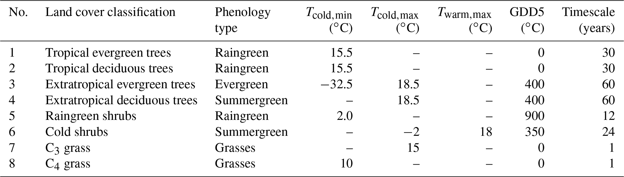
The occurrence of each PFT is limited by temperature constraints that reflect the bioclimatic tolerance of the individual PFTs. These environmental thresholds represent the chilling requirements of the plants by the maximum mean temperature of the coldest month (Tcold,max) and the cold resistance of the plants by the minimum mean temperature of the coldest month (Tcold,min). Furthermore, the presence of the PFTs is regulated by their heat requirements during their growth phase. This limit is realized by temperature sums over days on which mean temperature exceeds different thresholds (0 and 5 ∘C), called growing degree days (GDD0 and GDD5, respectively). Cold shrubs are also not able to survive in too-warm climates and are limited by the maximum mean temperature of the warmest month (Twarm,max). The different bioclimatic limits for the individual PFTs are listed in Table 1.
In addition to these limits, the dynamics of changes in the fractional coverage of PFTs in response to climatic change are governed by the dynamics of the net primary production (NPP) of the competing PFTs. The timescales of NPP dynamics include timescales for allocation, mortality and perturbation. The timescales of allocation and mortality are the same for each individual PFT but differ between PFTs. They range from 50 years for extratropical trees to 1 year for grass (see Table 1). If climate changes and if different PFTs can exist within the range of climate variability, then the PFT with the strongest NPP dominates, and the timescale of the transition mainly depends on the difference in the NPP allocation of the competing PFTs. If this difference is small, the transition is slow. The transition can be faster if one of the PFTs has much shorter timescales of allocation and mortality. The fastest changes occur if the climate crosses a bioclimatic threshold (see Table 1) or if a large-scale perturbation, such as windbreak or fire, occurs. Then, the PFT affected decays exponentially within a few decades or less.
The fractional PFT coverage of a grid cell can also change if the bare soil fraction (BSF), which represents the seasonal and permanently non-vegetated ground, varies. The BSF is determined by the relation of the carbon actually stored in the carbon pool for living tissues via the NPP of the individual plants to the maximum yearly carbon storage in this pool. This maximum is defined by the carbon costs needed by the plants to build up the leaves, stems, etc. completely and depends on the ratio of the maximum leaf area index to the specific leaf area of the PFTs.
2.3 Transient simulation
To run the model in quasi-equilibrium between early mid-Holocene boundary conditions, climate and the carbon cycle, a spin-up simulation has been performed with all forcings fixed to the values of the year 6000 BCE. This simulation was initialized from the pre-industrial climate and vegetation state and was run for more than 1000 years. The transient simulation then started from this equilibrium state and continued until pre-industrial times (i.e. 1850 CE). The transient simulation used in this study has been performed nearly identical to the simulation described in Bader et al. (2020), Brovkin et al. (2019) and Dallmeyer et al. (2020). The following forcings were prescribed:
- a.
Orbital-induced insolation changes (Berger, 1978), updated every decade. These mainly impact the seasonal cycle of, e.g. temperature and precipitation. The seasonality increases in the Southern Hemisphere and reduces in the Northern Hemisphere during the Holocene.
- b.
Greenhouse gas concentration (methane, carbon dioxide and nitrous oxide) inferred from ice-core records (Fortunat Joos, personal communication, 2016; see Brovkin et al., 2019; Köhler, 2019), updated every decade. The difference in CO2 between start and end of the simulations amounts to approximately 20 ppm.
- c.
Stratospheric sulfate aerosol injections imitating volcanic eruptions, prescribed from the Easy Volcanic Aerosol (EVA) forcing generator (Toohey et al., 2016), read annually, but calculated daily by linear interpolation. This forcing has been reconstructed based on ice-cores from both hemispheres to better identify volcanic eruptions with global impact on the climate. From Greenland, we employed sulfate data from the Greenland Ice Sheet Project 2 (GISP2; 72.97∘ N, 38.80∘ W) ice core (Mayewski et al., 1997). From Antarctica, we used sulfate data from the European Project for Ice Coring in Antarctica (EPICA) Dronning Maud Land (EDML; 75.00∘ S, 00.07∘ E) and Dome Concordia (EDC; 75.10∘ S, 123.35∘ E) ice cores (Severi et al., 2007), as well as sulfur and sulfate data from the WAIS (West Antarctic Ice Sheet) Divide ice-core project (WD; 79.48∘ S, 112.11∘ W) (Cole-Dai et al., 2021). These four ice cores were synchronized to the WD2014 chronology (Sigl et al., 2016) and volcanic sulfate mass deposition rates over Greenland and Antarctica were estimated using established methods (Sigl et al., 2014, 2015). Using the methodology developed (Gao et al., 2007) and applied to a similar bipolar network of ice cores over the past 2500 years (Toohey and Sigl, 2017), we estimated stratospheric sulfur injection (SSI) for in total 528 volcanic eruptions. Conversion of SSI into the aerosol properties is performed with the Easy Volcanic Aerosol module (Toohey et al., 2016). Aerosol extinction is assumed to be linearly proportional to mass for eruptions smaller than the 1815 Tambora eruption and follows a two-thirds power-law scaling for larger eruptions (Crowley and Unterman, 2013). The previous volcanic forcing reconstruction used in Bader et al. (2020) was based on a Greenland ice core (GISP2, Zielinski et al., 1996) only and therefore overestimated the effect of Icelandic and other extratropical volcanic eruptions on the global climate.
- d.
Spectral solar irradiance forcing includes an extrapolated 11-year solar cycle based on sun-spot observation datasets of far-infrared, near-infrared and visible radiation (Krivova et al., 2011), read annually, but calculated daily by linear interpolation.
- e.
Land use has been prescribed according to the LUH2 land-use dataset by Hurtt et al. (2020); it conforms to the CMIP6 simulations, is read annually, but is calculated daily by linear interpolation. This forcing begins 850 CE with a quasi-linear transition period (1000 years) starting 150 BCE to slowly build up the land use. Bader et al. (2020) used a preliminary (unpublished) version of the LUH2 dataset.
In the analysis of this study, the period 6000 to 150 BCE is considered only, to exclude the effect of land use on the vegetation distribution in the model. For easier nomenclature, we define the early mid-Holocene time slice (further referred to as 8 ka) by the climatological mean of the first 100 years of this transient simulations (i.e. years 6000–5901 BCE) and the late Holocene reference period (further referred to as 2.15 ka) by the climatological mean of the last 100 years of this simulations without land use (i.e. years 250–150 BCE). Accordingly, we define the 6 ka time slice by the climatological mean of the years 4000–3901 BCE.
2.4 Analysis methods
To summarize Holocene vegetation change, we choose the fuzzy c-means clustering technique (Bezdek, 1981). This method calculates a set of independent cluster centres (here: time series of vegetation development), such that the sum of the square distances between the items assigned to the cluster and the cluster centre is minimized. This means that grid cells showing similar vegetation changes over the course of the Holocene are grouped into the same cluster. We here use the c-means clustering function in R (Meyer et al., 2017) and calculate the cluster on the basis of 100-year running mean time series for the “forest”, “shrubs”, “grass” and “bare soil” PFT groups. The number of independent clusters has been optimized by the Xie–Beni method (Xie and Beni, 1991).
To test the most important climatic driver in the different regions, we performed a constrained ordination via the redundancy analysis function “rda” implemented in the “vegan” package of R (Oksanen et al., 2018).
The redundancy analysis (RDA) is an extended multiple linear regression method and measures the linear relationship between a set of response variables (here the PFT groups “forest”, “grass” and “shrubs”) and explanatory variables (here precipitation, temperature of the warmest month and temperature of the coldest month). It ordinates the vegetation on axes that are constructed in such a way that their relationship to linear combinations of the climate variables is maximized. Therefore, the RDA technique can also be seen as a constrained version of the principal component analysis. In this study, it is taken as a measure of the variation in vegetation that can be explained by the climate variables. The temperature of the coldest month explains only a small part of the variance in an initial RDA and was thus excluded in the final RDA shown here.
To assess the change in monsoon strength during the Holocene, we calculated the global monsoon area and the global monsoon precipitation following Zhou et al. (2008) with the modifications of Liu et al. (2009). In this definition, monsoon areas are characterized by a precipitation maximum (> 55 % of the annual total) in the summer season and a large annual range in rainfall. The summer season includes the months May to September for the Northern Hemisphere and the months November to March for the Southern Hemisphere. The reverse is applied for the respective winter season. As “annual range” the difference between summer and winter precipitation is taken. The monsoon precipitation is given by the sum of total summer rainfall in the monsoon area, taking the latitudinal changes in the grid-cell area into account.
For some analyses, seasonal means are considered. We are aware of the fact that the length of the season changes during the Holocene due to the precessional cycle (cf. Bartlein and Shafer, 2019). However, this does not change the response of the atmospheric physics in the model to the insolation change, so we assume that the results are not affected by a fixed calendar. But please keep in mind that we define the seasons according to the modern calendar implemented in the model; i.e. any statements regarding seasonal changes only refer to the simulation and might not necessarily be transferable to the real Holocene seasonal changes.
So far, palaeovegetation reconstructions have mostly been synthesized by biome distributions for individual time slices (e.g. Harrison, 2017; Cao et al., 2019a). Quantitative vegetation reconstructions are only available for few regions (e.g. Trondman et al., 2015; Cao et al., 2019b; Li et al., 2020). Therefore, we decided to evaluate the simulated vegetation against pollen-based biome reconstructions for the mid-Holocene (6 ka). The simulated PFT cover fractions were converted into mega-biome distributions using the approach by Dallmeyer et al. (2019). The agreement was tested by using the best neighbour score (BNS, Table 2; cf. Dallmeyer et al., 2019) that also considers the agreement in the surrounding grid cells of the record sites.
Table 2Best neighbour score (BNS) showing the agreement between pollen-based reconstructions and the mega-biomes converted from the simulated plant functional type cover fractions. Values between 0.2 and 0.5 mean “fair to good” agreement, above 0.5 “good to very good” agreement and above 0.8 “excellent” agreement. For details on the metric, see Dallmeyer et al. (2019).
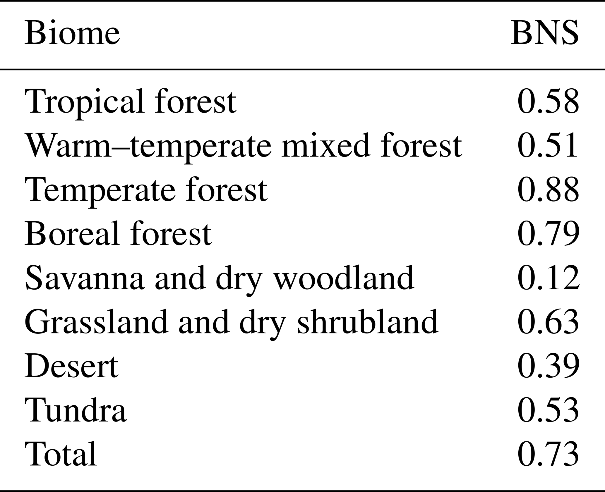
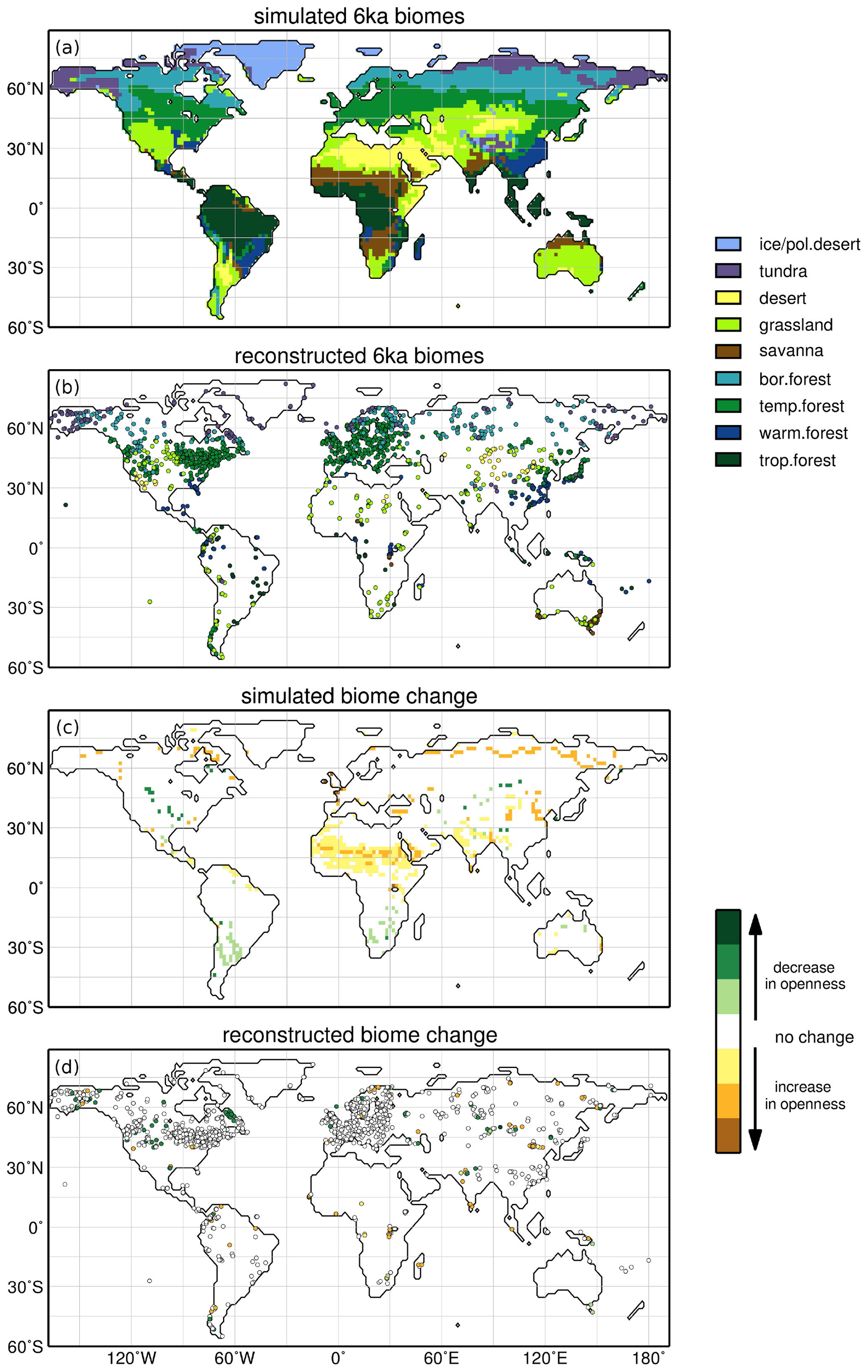
Figure 1Simulated (a) and reconstructed (b) biomes for the 6 ka time slice and the simulated (c) and reconstructed (d) change in vegetation between 6 ka and the pre-industrial (PI) era, expressed in terms of landscape openness. To assess the biome change, the biomes have been further grouped into the main categories of forest, savannas, grassland/tundra and desert. A decrease in openness describes the transition from biomes indicating more open landscape to biomes indicating less open landscape (e.g. desert in 6 ka to grasslands or to savannas or to forests in PI). Increase in openness of negative development describes the opposite transition (e.g. from grassland in 6 ka to desert in PI).
In principle, the vegetation in the model is well in line with the reconstructions (BNS of 0.73, Fig. 1). All major biome belts are reproduced. In particular, the extratropical forest biomes are well represented, showing a BNS of 0.79 (boreal forest) and 0.88 (temperate forest). The simulated deserts (BNS of 0.39) and savannas (BNS of 0.12) show little correspondence with the reconstructions. This is related to the fact that also in this simulation the northward spread of vegetation into the Sahara during the mid-Holocene is underestimated compared to the reconstructions (cf. Dallmeyer et al., 2020). Furthermore, the extent of the desert area in central Asia is too small. The reconstructed desert in the southwest of North America (mainly around the Mojave and Sonoran desert) is not reflected in the model. Very few reconstructions exist for the savanna regions, probably biasing the comparison. However, the method for biomizing PFTs has shortcomings in mapping savannas as this biome can hardly be delimited by climatic constraints and PFT compositions (cf. Dallmeyer et al., 2019). Tropical savannas can only be distinguished from forests by, e.g. their fire and shade tolerance and unique functional ecology (Ratman et al., 2011).
To analyse the main change in biomes towards PI, the biomes were further grouped into the main categories forests, savannas, grassland/tundra and deserts. Figure 1c–d show qualitatively the simulated and reconstructed difference for these biome categories between 6 ka and PI on the basis of the change in openness. Decrease in openness designates the transition from a more open landscape to a tree-dominated landscape (e.g. desert in 6 ka to grassland, grasslands to savannas or to forests in PI). Similarly, increase in openness refers to the transition from tree-dominated biomes to a more open landscape (e.g. forest in 6 ka to grassland in PI).
Since not all reconstructions mapped for 6 ka reach into pre-industrial times, we also considered PI records in the grid cells surrounding those of sites mapped in 6 ka. This method does not lead to a significant improvement of the record density in the difference plot. Therefore, we retained the original selection, i.e. showing only records with a counterpart at PI. Both the model and the reconstructions show only little change in the area covered by these main biomes. Most remarkable is the decrease in forest and grassland in the northern hemispheric monsoon regions and the decrease of forest along the taiga–tundra boundary in the high northern latitudes indicated by the model. The reconstructions in principle also suggest this development, even if the record density is too low to show a detailed picture, particularly in north Africa.
The decrease in openness in central North America and central Asia is visible in the model and in the reconstructions. The records furthermore suggest a greening at the Labrador Sea coast, which is not shown by the model. This may be related to the migration of plants after the retreat of the Laurentide Ice Sheet. The changes in land ice coverage are not considered in the model so this process cannot be represented. The model indicates a decrease in openness in the southern African and South American extratropics. This is not seen in the records showing rather no change in main biome category, but only few records exist that are located directly in the regions in which the model shows this positive signal. Hence our prediction, or hindcast, awaits further evaluation.
The simulated Holocene vegetation change from 8 to 2.15 ka has been clustered on the basis of the 100-year running mean time series. The desert and forest change can be grouped into four and the shrubs and grass change into five different clusters (Fig. 2). Figure 2a, c, e, h mark the regions that can be assigned to the respective cluster. Figure 2b, d, f, g show the trends in the respective cluster centre. Overall, the Holocene vegetation changes in this global view are quite linear, overlaid by weak multi-centennial variability. However, non-linear changes in PFTs may occur on local or regional level. The most striking vegetation shifts seen in Fig. 2 are
- a.
a strong decrease in forest and increase in grass and shrubs in the high northern latitudes reflecting the southward retreat of the northern treeline and the shift from taiga forest to tundra;
- b.
a (strong) increase in the subtropical northern hemispheric deserts coinciding with a decrease and equatorward retreat of all vegetation types in the monsoon regions;
- c.
an increase in the vegetated area in extratropical North America (mainly 300–60∘ N, 90–120∘ W) related to an increase in forest and partly grass;
- d.
an increase in the vegetation in extratropical South America and southern Africa due to an increase in forest, grass and shrubs (southern Africa), including the southern hemispheric monsoon regions; and
- e.
a bipolar vegetation change in Australia, mostly driven by an increase in grass on the northern and a decrease of grass on the southern part of the continent.
Figure 3 shows a similarly calculated cluster analysis for the 100-year running means of annual mean precipitation and the temperature of the warmest and coldest months, respectively, assuming that these variables are the main climatic factors affecting the vegetation change. In line with the increasing wintertime insolation during the Holocene, the temperature of the coldest month (Tcold) uniformly increases in the Northern Hemisphere, in particular on the continents by up to 1.6 K (cluster centre). In the Southern Hemisphere, Tcold only changes in a few grid boxes in southern Africa and in the northern part of Australia, showing an overall decreasing trend with strong millennial variability.
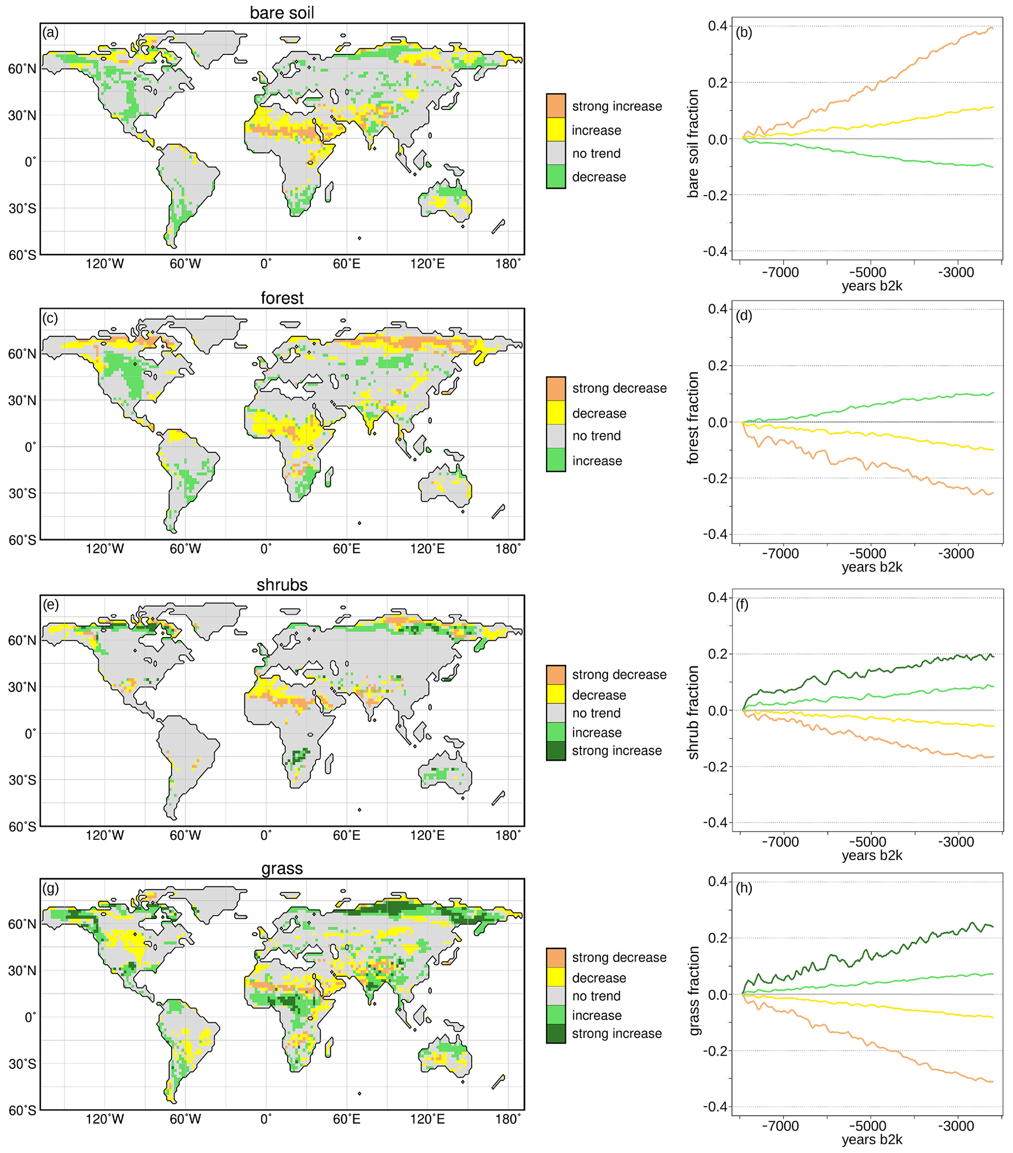
Figure 2Simulated Holocene vegetation cluster, derived by the c-means clustering method (R, Meyer et al., 2017). The left panel displays the cluster pattern for (a) the bare soil cover, which is 1 minus the total vegetation in the model, (c) forest cover, (e) shrub cover and (g) grass cover. The right panel shows the respective trends in the cluster centres, i.e. for (b) bare soil fraction, (d) forest fraction, (f) shrub fraction and (h) grass fraction. For the analysis, 100-year running means of the anomaly time series (fraction at certain time step – 8 ka climatological mean) have been taken. The cover fraction change of the cluster centres can range from −1 to 1 in the model, i.e. decrease of 100 % or increase of 100 %, respectively.
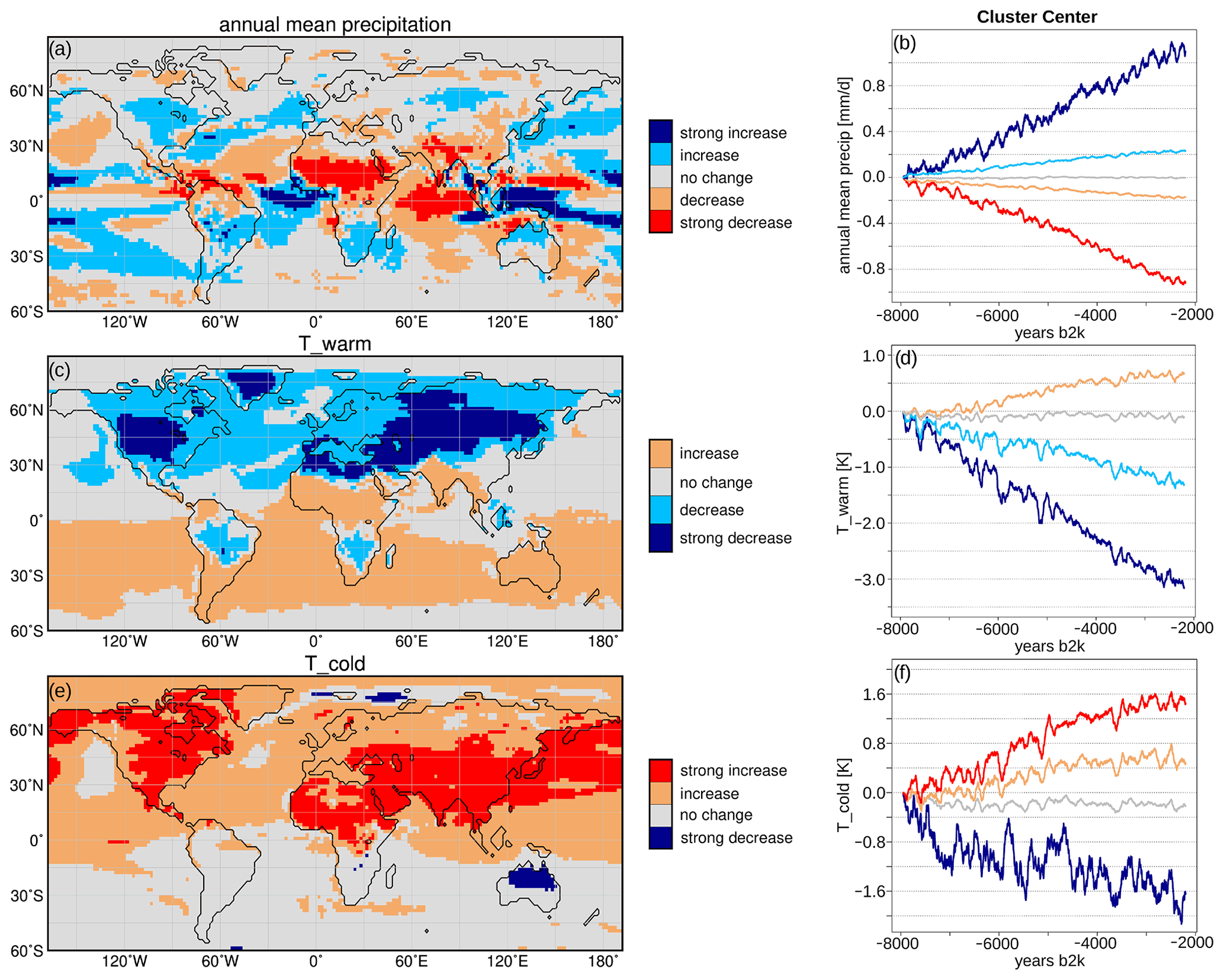
Figure 3Simulated Holocene climate cluster, derived by c-means clustering method (R, Meyer et al., 2017). The left panel displays the cluster pattern for (a) annual mean precipitation, (c) temperature of the warmest month (Twarm) and (e) temperature of the coldest month (Tcold). The right panel shows the respective trends in the cluster centres, i.e. for (b) annual mean precipitation (mm d−1), (d) Twarm (K) and (f) Tcold (K). For the analysis, 100-year running means of the anomaly time series (value at certain time step – 8 ka climatological mean) have been taken.
The temperature of the warmest month (Twarm) shows the opposite trend, in line with the summertime insolation change. Twarm decreases in the Northern Hemisphere, particularly in the continental midlatitudes (up to 3.2 K). In the Southern Hemisphere, Twarm increases moderately during the Holocene by 0.7 K. The signal is reversed in the tropical monsoon areas, probably due to a drop in evaporative cooling in the northern and an increase in evaporative cooling in the southern hemispheric tropical monsoon regions. Both Twarm and Tcold are intercepted by relatively strong “events”, leading to a drop in temperature in all cluster centres by up to 0.7 K for several hundred years. These events may at least partly be associated with the volcanic forcing prescribed to the model. The Pearson correlation coefficient between the detrended Twarm cluster centres and the volcanic forcing ranges from 0.6 (for the increasing cluster centre) to 0.8 (for the decreasing cluster centre). The Pearson correlation coefficient between the detrended Tcold cluster centres and the volcanic forcing ranges from 0.27 (for the decreasing cluster centre) to 0.74 (for the increasing cluster centre). These events have hardly any effect on the general vegetation trends.
In contrast to the hemispheric uniform temperature trends, the annual mean precipitation (Pann) varies at regional level. Pann increases in large parts of North America and in central northern Asia (approximately 45–60∘ N, 70–110∘ E). In the northern hemispheric monsoon regions, precipitation decreases, particularly in the north African monsoon domain and the southern rim of the Himalayas.
In the Southern Hemisphere, Pann increases in the monsoon region and the extratropics with the exception of Australia showing a decline in precipitation at the eastern coast and no change in the central and western parts (south of 22∘ S). The signal in the continental monsoon domains is well in line with the orbital monsoon hypothesis (Kutzbach, 1981) that directly links an increase in summer insolation with a strengthening of the summer monsoons, and vice versa. Pann also increases in northern Brazil and along the western coasts of the South American continent and southern Africa. Precipitation does not change much north of 60∘ N, which implies that the shifts in vegetation distribution are rather controlled by temperature changes in this region.
To test the most important climatic driver in the different regions, we performed a constrained ordination via the redundancy analysis function “rda” implemented in the “vegan” package of R (Oksanen et al., 2018).
Figure 4 summarizes the results, qualitatively showing the main contributors (Twarm vs. Pann) explaining the variance in the vegetation change. The temperature of the coldest month explains only a small part of the variance in an initial RDA and was thus excluded in the final RDA.
The RDA result confirms that temperature is the most important variable constraining the vegetation change in the high northern latitudes, with the exception of East Siberia where the decrease in forest can only be explained by the combined effect of Pann and Twarm. The shared variance of both variables is higher than the unique contribution by Twarm. Also, in most other regions, both variables jointly explain the vegetation dynamics during the Holocene (not shown), but in most regions, precipitation contributes most (Fig. 4). Variations in Twarm are only important in the maritime areas of the Northern Hemisphere, where changes in vegetation are generally very small (i.e. cluster centre shows no change), in western Canada, central-west Brazil, Patagonia, equatorial Africa and around the Tibetan Plateau.
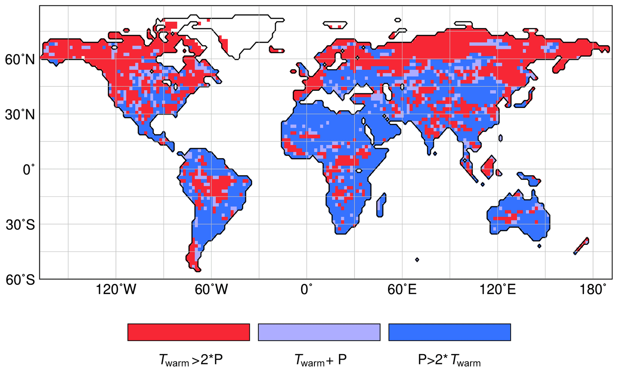
Figure 4Results of the redundancy analyses performed by the “vegan” routine in R (Oksanen et al., 2018) for the vegetation groups forest, shrubs and grass, with precipitation (P) and temperature of the warmest month (Twarm) as explanatory variables. This figure is based on the ratio of the variance explained by Twarm and by precipitation. When P > 2 × Twarm, then precipitation explains more than twice as much of the variance as Twarm, and vice versa for Twarm > 2 × P.
This pattern of climate drivers resembles the findings by Seddon et al. (2016) analysing the effect of cloudiness, temperature and precipitation on recent vegetation productivity based on satellite data. In their study, temperature is also the most influential factor in the high northern latitudes, whereas elsewhere precipitation explains most of the vegetation variability. In north Africa and the northern part of South America, the climatic driver is not as pronounced as in our RDA analysis, but the results can only be compared to a limited extent, as the modern data are influenced by land use that is excluded in our analysis.
Although the shared variance accounts for the largest part, precipitation in all monsoon regions explains much more of the vegetation change than Twarm. Given the uniform hemispheric trend in temperatures, precipitation is the factor that imprints the regional variations on the vegetation signal. We therefore focus on analysing the precipitation change as the main driver of the global vegetation trend rather than disentangling the temperature signal whose sign is directly forced by the Holocene insolation change. The simulated vegetation distributions for 2.15 and 8 ka are displayed in Appendix A. Reference maps for the 2.15 ka climate states can be found in Appendix B.
5.1 The northern hemispheric monsoon domain
In both hemispheres, warm season precipitation is the most important driver of the Holocene precipitation signal (Fig. 5). For the global monsoon domains, this is well in line with the orbital monsoon hypothesis (Kutzbach, 1981). The rise in northern hemispheric summertime insolation during the early Holocene leads to a strengthening of the thermal gradient between the continents and the oceans, enhancing the monsoon circulation and increasing the summertime precipitation over land. Climate model simulations and reconstructions indicate an increase in moisture availability in the monsoon margin regions and an inland penetration of the vegetation belts (Jolly et al., 1998; Hély et al., 2014; Feng et al., 2006; Zhao et al., 2009; Metcalfe et al., 2015). In the Southern Hemisphere, the decrease in insolation generally leads to a weakening of the monsoon circulation over land and the opposite effect on precipitation and vegetation (Wang et al., 2014, and references therein).

Figure 5Season which contributes most to the annual mean precipitation change between 8 and 2.15 ka in the model, i.e. September to November (SON), June to August (JJA), March to May (MAM) and December to February (DJF). Please note that the seasons are calculated on the fixed model calendar and are not adjusted to the astronomical forcing (cf. Bartlein and Shafer, 2019).
To assess the change in monsoon strength, we calculated the global monsoon area and the global monsoon precipitation following Zhou et al. (2008) with the modifications of Liu et al. (2009) (cf. Methods section).
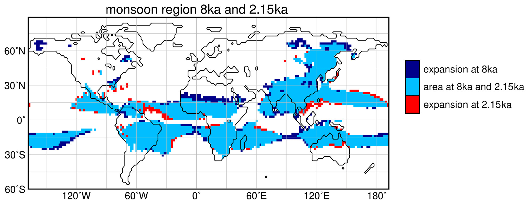
Figure 6Monsoon region at 8 ka and 2.15 ka, derived by the method by Zhou et al. (2008) with the modifications by Liu et al. (2009). The figure shows the monsoon area that is indicated for both time periods, i.e. the area that does not change from mid- to late Holocene (light blue), the area additionally assigned to the monsoon domain at 8 ka but not at 2.15 ka (dark blue) and the area additionally assigned to the monsoon domain at 2.15 ka but not at 8 ka (red).
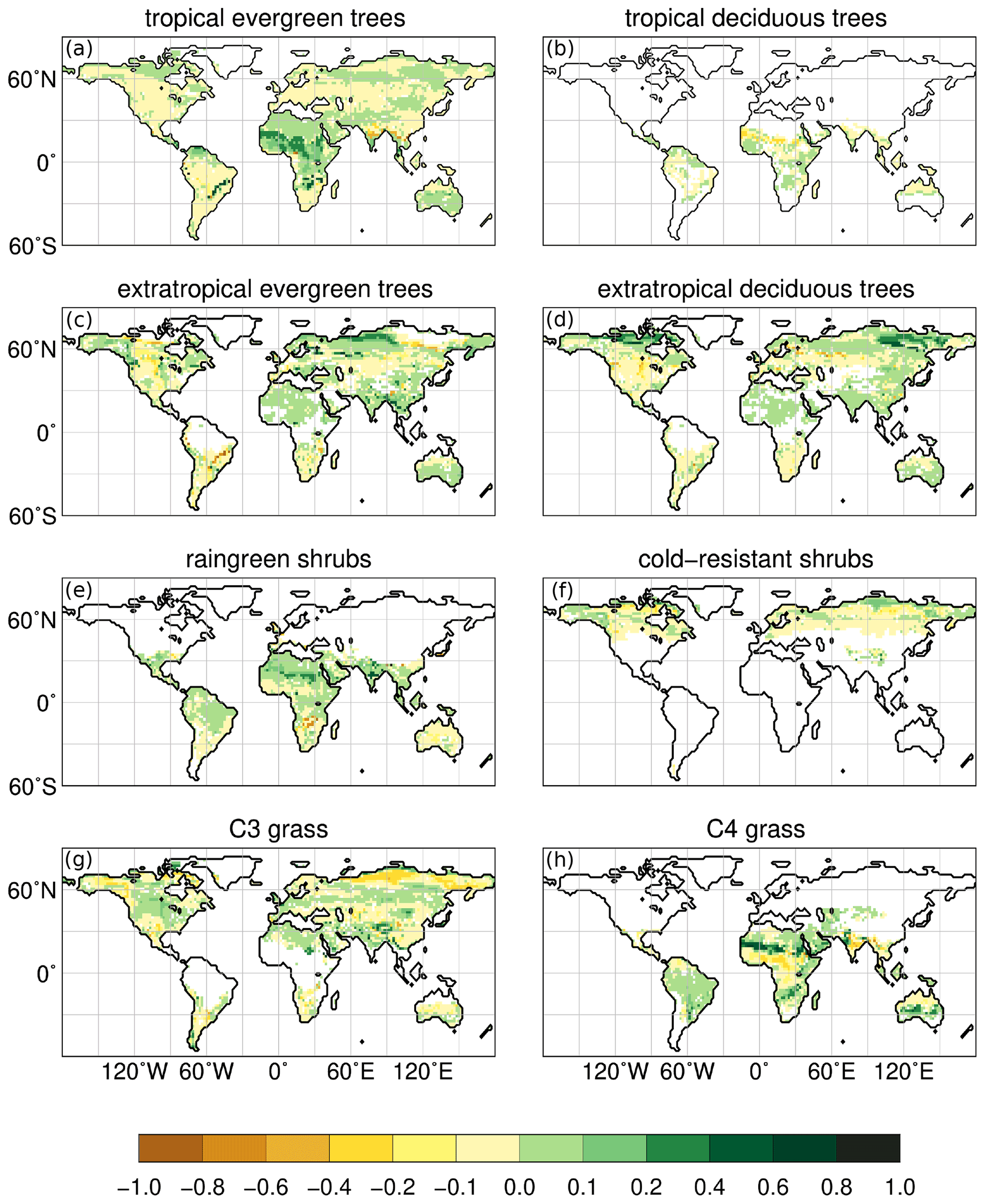
Figure 7Simulated changes in PFTs for the early mid-Holocene time slice (at 8 ka) compared to the late Holocene (2.15 ka); i.e. the yellowish colour indicates a decreased in PFT cover fraction at 8 ka, greenish colour an increased PFT cover fraction at 8 ka compared to 2.15 ka. Values of “1.0” mean that the grid box is fully covered by the PFT during 8 ka, but does not occur at 2.15 ka in this grid cell, and vice versa for values of “−1.0”. Only significant changes are shown (t test, 99 % confidence interval).
According to our model, the northern hemispheric monsoon region is expanded by more than 25 % on the continents at 8 ka compared to 2.15 ka (Table 3, Fig. 6). The monsoon precipitation is increased by 40 % over land. With a northward expansion of about 600 km (up to 22∘ N), the north African monsoon area is the most enlarged monsoon domain during 8 ka. This coincides with a vegetation expansion into the Sahara at 8 ka. In the extended monsoon area, raingreen shrubs are increased by up to 30 % (Fig. 7e) and the grass fraction by up to 60 %, reflected by the cluster centres with strong decreasing trend over the Holocene (cf. Fig. 2). Raingreen shrubs populate the entire western Sahara and reach a coverage of about 10 % in large parts, going up to 20 % in the coastal regions at 8 ka (Figs. 7e and A2 in Appendix A). In the eastern Sahara, they are spread out substantially to only about 24∘ N. At the northwestern monsoon boundary, the forest cover fraction is decreased during 8 ka. This is related to the colder northern hemispheric winter climate during the mid-Holocene leading to unfavourable growth conditions for tropical trees in these grid cells. The temperature of the coldest month is around 15.5 ∘C, which is a fixed bioclimatic limit for tropical trees in the model. With the continuous boreal winter warming towards PI, cold season temperature exceeds this limit more and more, leading to an establishment of tropical deciduous trees. The overall non-vegetated area north of 15∘ N is diminished by 22 % in the mean at 8 ka, ranging up to 82 % in the central Sahel. Thus, the vegetation changes in our model are significantly stronger and more expanded into the Sahara than in other recent global climate model simulations (e.g. Rachmayani et al., 2015; Hopcraft et al., 2017).
Table 3Simulated change in northern hemispheric (NH) and southern hemispheric (SH) monsoon area and monsoon precipitation for the mid-Holocene (8 ka) compared to the late Holocene (2.15 ka). The changes have been calculated following the method of Zhou et al. (2008) with the modifications of Liu et al. (2009).

In the core monsoon domain (0–15∘ N), total vegetation cover is not increased during the early mid-Holocene, but tropical evergreen trees are much more widespread (Fig. 7a). In the course of the Holocene, these forested areas are replaced by grassland. Tropical eastern Africa experienced an increased total vegetation cover during the early mid-Holocene that is determined by an enhanced monsoon related moisture flux convergence in spring in the model (not shown) leading to an expansion of grass covered areas. This is in line with general higher early and mid-Holocene moisture levels in large parts of tropical eastern Africa as shown, e.g. in lake-level reconstructions (see overview by Tierney et al., 2011).
In the other northern hemispheric monsoon domains, the vegetation change is more regionally confined. The East Asian monsoon area is expanded to the northwest into western Mongolia by up to 800 km at 8 ka compared to 2.15 ka (Fig. 6). This leads to an increased in total vegetation cover by up to 27 % per grid cell, mainly due to an expansion of the grass cover (Fig. 7g). The cover fraction of the extratropical deciduous and evergreen trees is also increased in total, although in several grid boxes it is only one tree PFT being replaced by the other. Pollen-based reconstructions reveal a regionally strongly increased tree cover fraction during the mid-Holocene, particularly in the middle and lower reaches of the Yellow River (Ren, 2007; Tian et al., 2016). This is also the area in which our model indicates the largest changes in tree cover. Over the course of the Holocene, the vegetation belts retreat back to their modern position, coincident with the monsoon retreat, so that the grass fraction at the eastern rim (approximately 41–46∘ N, 117–120∘ E) increases towards 2.15 ka at the expense of the tree cover fraction (Fig. 7c, d).
The South Asian monsoon is expanded at its northwestern rim by about 1–2 grid cells (approximately 200 km) into western South Asia and onto the Tibetan Plateau (Fig. 6), leading to a bare soil fraction decreased by up to 50 % at 8 ka. The enhanced monsoon coincides with a widespread increase in area covered by raingreen shrubs, extratropical evergreen trees and grassland, in particular on the Tibetan Plateau and along its eastern margin, along the Gulf of Kutch, and in the Thar Desert during the early mid-Holocene (Fig. 7). Tropical evergreen forest are decreased along the western coastal region of South Asia due to temperature limitations in the cold season. Our model reveals less vegetation in central South Asia (17.5–21.5∘ N, 75–82.5∘ E) during the early mid-Holocene, driven by a tropical evergreen forest cover decreased by up to 50 % and a C4 grass cover reduced by up to 35 %. Partly, these PFTs are replaced by raingreen shrubs and C3 grass at 8 ka, reflecting a cooler winter climate. This region is close to sites at which reconstructions reveal a less humid climate and more open landscape during the early mid-Holocene compared to the late Holocene (Chauhan et al., 2013). Our model shows rather decreased precipitation levels (less significant) at 8 ka summers, caused by a high-pressure anomaly in the lower atmosphere above South Asia and Indochina (Fig. 8d). The anticyclonic atmospheric flow around this anomaly exhibits low-level easterly wind above southern India (Fig. 8c), inhibiting the moisture flux to central South Asia. Furthermore, the high-pressure anomaly is associated with strong subsidence (Fig. 8a). The monsoon flow stretches more to the north at 8 ka compared to 2.15 ka. All these factors lead to a decreased moisture availability in this region, worsening the climatic conditions for the establishment of vegetation in the model during the early mid-Holocene.
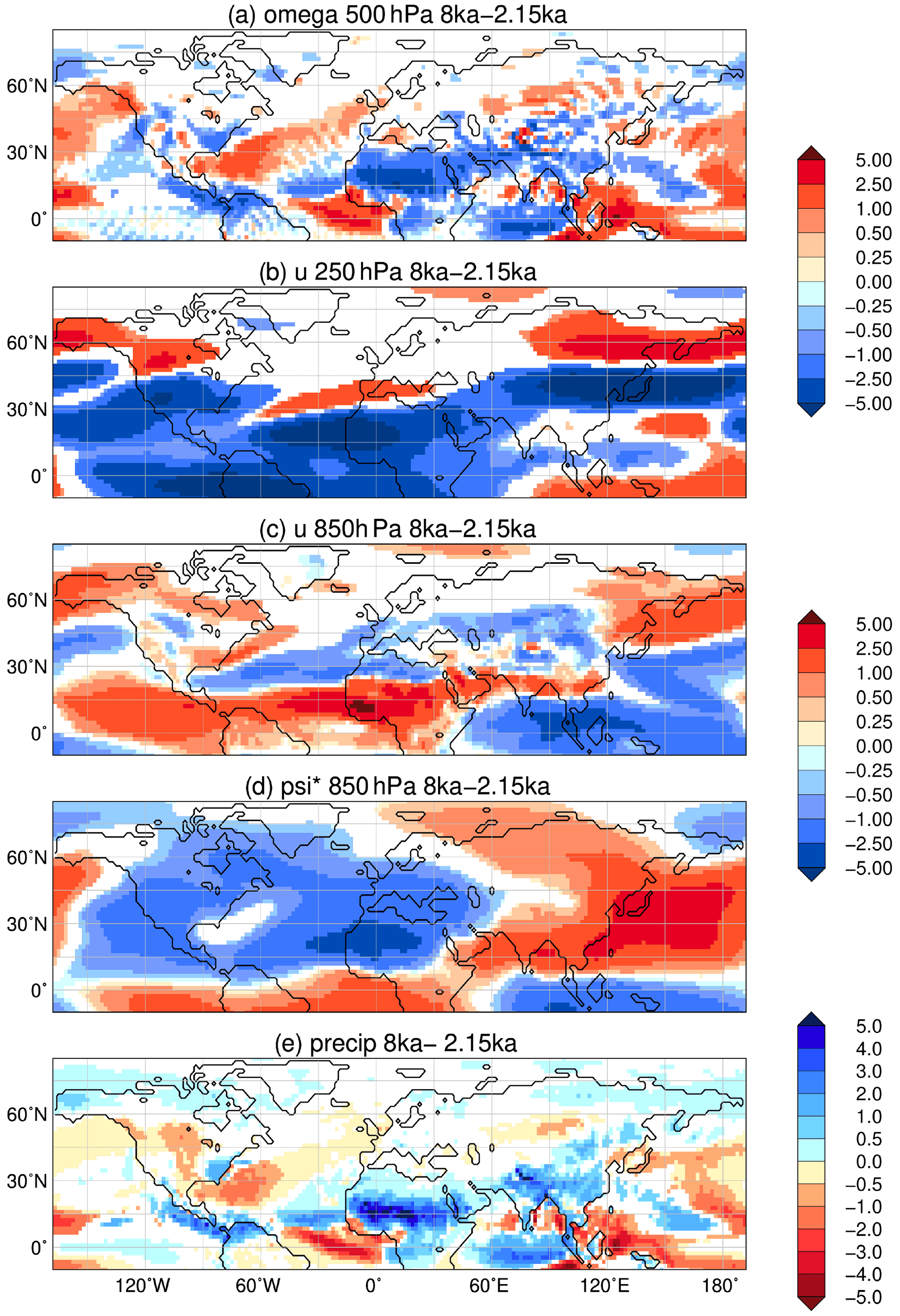
Figure 8Simulated difference in June to August (JJA) mean climate in the model for the time slice 8 ka compared to 2.15 ka, i.e. (a) vertical velocity (omega) in 500 hPa (10−2 m s−1) with blue colour showing increased uplift during 8 ka; (b) upper-tropospheric zonal wind (u) in 250 hPa (m s−1) with blue colours indicating enhanced easterly wind; (c) low-level zonal flow (u) in 850 hPa (m s−1); (d) zonal anomaly in lower-tropospheric streamfunction (psi*, in 107 m2 s−1) reflecting the change in standing waves, with blue colours indicating increased cyclonic circulation at 8 ka compared to 2.15 ka; and (e) mean seasonal precipitation (mm d−1) with blue colours showing enhanced precipitation during 8 ka. Only significant changes are shown (t test, 99 % confidence interval).
The reduction in the South Asian monsoon strength during the Holocene also affects the vegetation on and around the Tibetan Plateau. At 8 ka, extratropical evergreen forests are more widespread along the northeastern and southwestern edge (Fig. 7c). On the Tibetan Plateau, grass cover is strongly increased compared to 2.15 ka (up to 40 %), owing to the higher summer precipitation (Fig. 8e). This pattern of changes is in line with pollen-based vegetation reconstructions (e.g. Herzschuh et al., 2010; Van Campo et al., 1996).
The North American monsoon area is expanded southward and westward by approximately 200 km during the early mid-Holocene (Fig. 6). Summer precipitation is substantially increased above the ocean, in Central America and the northwestern part of the South American continent, similar to that seen by reconstructions (Metcalfe et al., 2015). The increase in precipitation leads to a larger area covered by tropical evergreen forests in the model. In the course of the Holocene, tree cover reduces and is replaced by grass (Fig. 7).
5.2 The southern hemispheric monsoon domain
In total, the southern hemispheric monsoon domain is enlarged by 8 % and receives 7 % more precipitation at 8 ka compared to 2.15 ka. However, the continental monsoon area is smaller by 5 % and precipitation level only reaches 89 % of the 2.15 ka values (Table 3). Thus, the changes in the strength of the monsoon during the Holocene are much smaller in the Southern Hemisphere than in the Northern Hemisphere. For example, the monsoon area in South America is reduced by only a few grid cells, mainly in the western part (Fig. 6) during the early mid-Holocene. Nevertheless, annual precipitation in nearly the entire continental monsoon area is lower at 8 ka than at 2.15 ka (Fig. 3), due to a generally northward displaced Intertropical Convergence Zone and diminished uplift of moist air over the central continent during the monsoon season (cf. Fig. 9). Both are also mirrored in the slightly increased precipitation on the northeasternmost continent (i.e. northeastern Brazil and the Caribbean region). This pattern is supported by reconstructions and other simulations (Maksic et al., 2019; Prado et al., 2013a, b; Cruz et al., 2009) for the mid-Holocene.
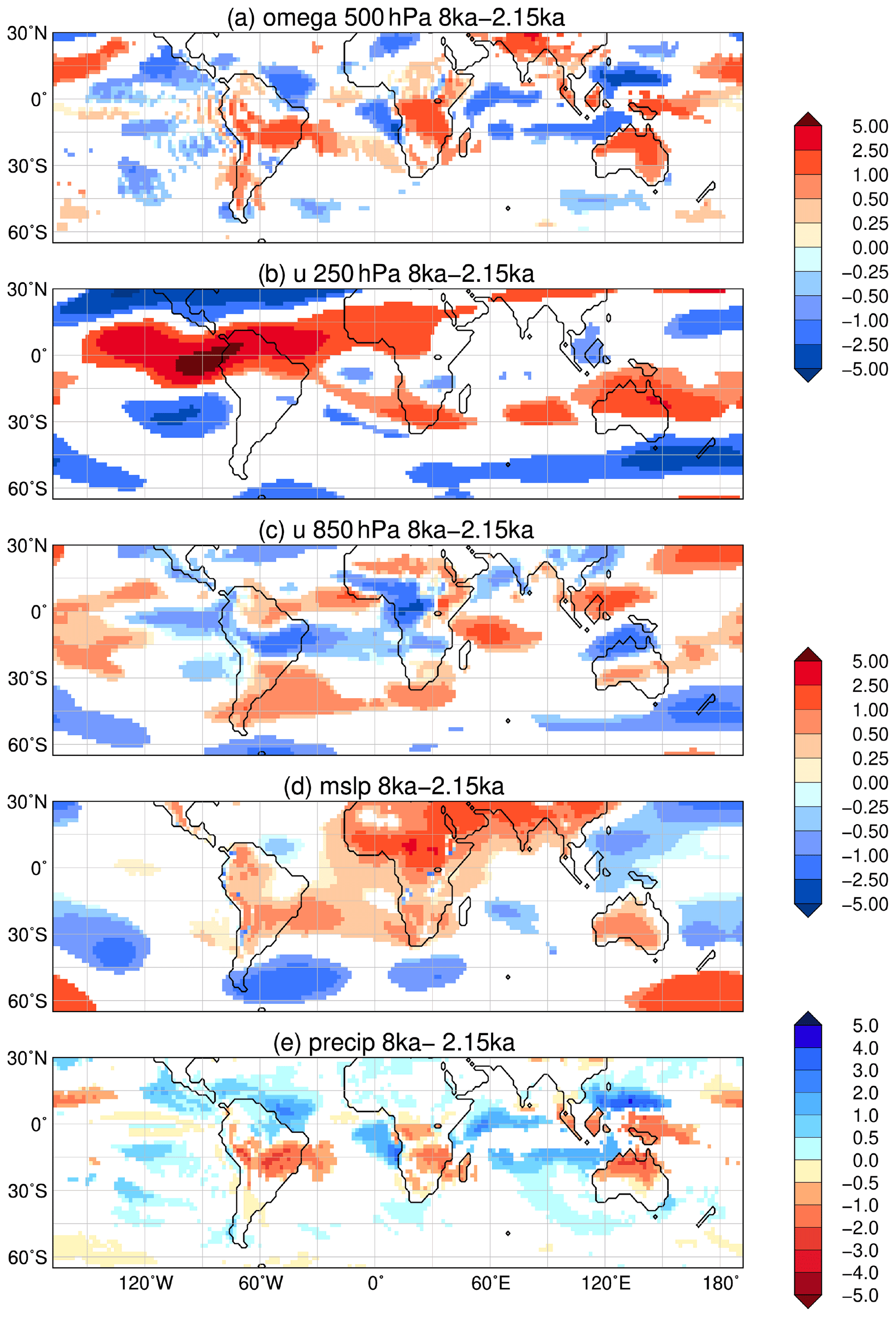
Figure 9Simulated difference in December to February (DJF, austral summer) mean climate in the model for the time slice at 8 ka compared to 2.15 ka, i.e. (a) vertical velocity (omega) in 500 hPa (10−2 m s−1) with blue colour showing increased uplift during 8 ka; (b) upper-tropospheric zonal wind (u) in 250 hPa (m s−1) with blue colours indicating enhanced easterly wind; (c) low-level zonal flow (u) in 850 hPa (m s−1); (d) mean sea level pressure (hPa) with low-pressure anomaly given in blue colours; and (e) mean seasonal precipitation (mm d−1) with blue colours showing enhanced precipitation during 8 ka. Only significant changes are shown (t test, 99 % confidence interval).
The reduced precipitation has a minor effect on the total vegetation cover that is only slightly decreased along the foot of the Bolivian Andes. The vegetation in the Amazon rainforest region is relatively stable, but forest is shrunk at its southern edge during the early mid-Holocene, confirming the picture revealed by reconstructions (e.g. Mayle et al., 2000; Mayle and Power, 2008; Rossetti et al., 2017). Outside of this region, it is rather the vegetation composition that changes. The cover fraction of tropical evergreen trees is increased by up to 86 % in a broad band in southeastern Brazil (Fig. 7a), which is overcompensated by a diminished fraction of extratropical evergreen trees and partly also extratropical deciduous trees. Thus, the total tree cover in this region is decreased and replaced by grassland at 8 ka compared to 2.15 ka, indicating a decreased Atlantic rainforest and more open vegetation similar as proposed in reconstructions (e.g. Ledru et al., 2009). In the model, this is the effect of a climate characterized by warmer winters, but that is still not moisture limited in the monsoon domain.
On the central continent (approximately 15–30∘ S, along 60∘ W), extratropical and tropical evergreen tree covers are diminished by up to 22 %, leading to less forested area during the early mid-Holocene. In this region, grass cover is slightly enhanced during 8 ka. This pattern of forest transitions fits well to a recent palaeorecord synthesis revealing the most significant Holocene transitions in vegetation for southwestern Amazonia and southeastern Brazil, induced by a less intense South American summer monsoon (cf. Smith and Mayle, 2018).
The precipitation on the southern African continent is diminished in the entire monsoon domain during the early mid-Holocene austral summer (Fig. 9e) as well as the annual mean (Fig. 3). This can mostly be attributed to the less powerful monsoon circulation at 8 ka compared to 2.15 ka. The Angola Low is weakened and the South Atlantic High is shifted northwards (Fig. 9d), reducing the moisture flux to the continent and thereby decreasing precipitation (cf. Vigaud et al., 2009). The relatively weaker South Indian High induces an anticyclonic circulation with a northerly wind anomaly along the coast and landward low-level winds (Fig. 9c). This leads to increased precipitation over the ocean and decreased precipitation over land at 8 ka. The ITCZ is weakened, coinciding with reduced uplift (Fig. 9a) and inhibited convection.
The South African monsoon area is reduced by about 200 km in its northwestern part (approximately 3.5–5.5∘ S, 14–24∘ E) at 8 ka (Fig. 6). This is related to the fact that the west African monsoon dynamics also imprint on the tropics in the Southern Hemisphere (up to approximately 10∘ S), probably due to easterly moisture-bearing trade winds off the Indian Ocean (e.g. Burrough and Thomas, 2013; Vincens et al., 2005). As a result, the tropical region not only experiences an increase in summer precipitation due to the intensification of the South African monsoon over the course of the Holocene but also a decrease in winter precipitation due to the weakening of the west African monsoon and easterly flux from the Indian Ocean (Fig. 8). Therefore the annual range of precipitation in this region is reduced during the early mid-Holocene, not fulfilling the criteria of monsoon areas used in this study.
The overall result of the change in precipitation is an increased cover fraction of tropical evergreen trees (up to 16 %) in parts of central (12–20∘ S, 20–29∘ E) and eastern (12–14∘ S, 31–36∘ E) Africa at 8 ka (Fig. 7a). Over the course of the Holocene, tree cover reduces and is replaced by grassland, in line with the tropical regions on the north African continent. South of 15∘ S, the vegetation change is more complex. The total vegetation is decreased in three north–south-orientated stripes, mainly due to a decreased grass cover at 8 ka. East of 30∘ E, extratropical trees are reduced during the early mid-Holocene and partly replaced by grassland. West of 30∘ E, tropical evergreen trees strongly recede over the course of the Holocene and give way to raingreen shrubs and C4 grass. This is probably also related to the bioclimatic limit for the temperature of the coldest month needed for the establishment of tropical trees in the model (Table 1) that is at some point in time no longer met in the cooling winter climate in the Southern Hemisphere during the Holocene. Southern Africa experiences rather an increase in C3 grass and extratropical trees from 8 ka to 2.15 ka, while raingreen shrubs slightly decrease (Fig. 7e).
Reconstructions show a diverse picture but rather show more humid vegetation types during the mid-Holocene and aridification afterwards (Olago, 2001; Burrough and Thomas, 2013, and references therein). This may at least partly be related to the fact that the vegetation distribution in southern Africa is strongly controlled by fires, maintaining grassland and savannas despite sufficient rainfall for the establishment of forest (Bond et al., 2003; Bond, 2008). JSBACH includes a fire model, but the effect of fires may be underestimated in the southern African region. At least southern African vegetation seems to be highly correlated with climate in our simulation.
The Australian monsoon region is shrunk at its southeastern rim by approximately 200 km at 8 ka (Fig. 6). The high-pressure anomaly above the continent leads to an anticyclonic flow with low-level westerly winds south of the monsoon domain (approximately 22∘ S) and easterly winds in the monsoon region (Fig. 9c). This results in a weakened monsoon-related moisture flux and less precipitation during austral summer during the early mid-Holocene in the model (Fig. 9e). Other climate model simulations reveal contradictory results with some even showing a stronger monsoon and increased precipitation during the mid-Holocene (e.g. Liu et al., 2004). In MPI-ESM, the total vegetation is decreased by up to 19 % in the north Australian monsoon region during the early mid-Holocene, mainly due to a decreased C4 grass cover and less tropical evergreen trees. On the southern edge of the monsoon domain, the tropical evergreen tree cover is raised by up to 20 % at the expense of extratropical evergreen trees and raingreen shrubs (Fig. 7). This switch between different woody PFTs is mainly determined by the warmer southern hemispheric winter climate during the mid-Holocene.
5.3 Extratropical North America
According to the model, the total vegetation cover in large parts of North America increases from 8 ka to 2.15 ka (Fig. 2). Most prominent is the vast expansion of trees, ranging from the southern Great Plains to the Canadian interior plains and the northeastern Rockies that is also seen in reconstructions (Grimm et al., 2001). In the model, this is manifested by a rise in the extratropical evergreen tree fraction by up to 24 % west of 100∘ W and a rise in extratropical deciduous tree fraction by up to 45 % east of 100∘ W (Fig. 7). During the early mid-Holocene, most of this region is covered by grassland or bare soil. In the southern Great Plains, raingreen shrubs are more widespread at 8 ka; these are replaced by grass during the Holocene.
The precipitation response to the orbital forcing in the model is a complex mixture of several interacting processes. In total, the Great Plains receive less precipitation during the early mid-Holocene (Fig. 3a). Figure 5 shows that the summer months contribute most to the annual mean precipitation change. These are also the months in which the northern hemispheric monsoon dynamics are most vigorous and the orbital forcing has the strongest imprint on the monsoon circulation. Summer monsoon precipitation coincides with a strong condensational latent heat release, affecting also the tropospheric circulation in the extratropics (e.g. Gaetani et al., 2011; Nakanishi et al., 2021). The subtropical anticyclones are stated to be related to Kelvin and Rossby wave responses to the heating in the monsoon rainband (Matsuno, 1966; Gill, 1980; Rodwell and Hoskins, 2001; Trenberth et al., 2000). These anticyclones cover about 40 % of the Earth's surface (Rodwell and Hoskins, 2001) and are therefore a major player in the global circulation of the atmosphere and oceans and the atmospheric teleconnection pattern. This suggests that the strong changes in the northern hemispheric monsoon systems also play a decisive role in modifying the extratropical vegetation change over the course of the Holocene. Figure 8d displays the mean change in the atmospheric standing waves during June, July and August (JJA). The Bermuda High is strengthened in the core at 8 ka leading to a rerouting of the moisture transport from the Gulf of Mexico along the Atlantic coast, thereby enhancing the precipitation along the Appalachian mountain range (cf. also Williams et al., 2010). In this region of raised precipitation levels, the extratropical deciduous tree fraction and with it the total forest cover is even higher during the mid-Holocene than at 2.15 ka.
The moisture flux is more divergent in the Great Plains and the atmosphere is generally drier, inhibiting convection and rainfall. The intensity change of the Bermuda High has so far been seen as one possible explanation for the change in Holocene vegetation pattern seen in pollen-based reconstructions (e.g. Grimm et al., 2001, and references therein). In addition, the model shows a rainfall-reducing subsidence anomaly over the Great Plains south of 45∘ N at 8 ka (Fig. 8a) that could at least partly be attributed to a Rodwell–Hoskins-like Rossby wave response to the enhanced updrafts in the North American summer monsoon (Harrison et al., 2003). The northward-shifted upper-level westerly jet during the mid-Holocene (Fig. 8b) coincides with a northward replacement of the storm tracks, which probably results in less transient eddy transport to the northern Great Plains at 8 ka (Seager et al., 2014). The model also reveals less precipitation during spring and therefore limited evaporation during mid-Holocene summer (not shown), reducing water recycling and the northward transport of moisture in the Great Plains low-level jet. The influence of evaporation on vegetation change may also explain the relatively large proportion of vegetation variance explained by the temperature of the warmest month (cf. Fig. 4).
The more La Niña-like sea surface temperature pattern (Fig. B1, Appendix B) may also contribute to the drier surface conditions in the Great Plains during the mid-Holocene, although the pattern is probably less pronounced in the model than indicated by reconstructions (Shin et al., 2006). Which of these mechanisms is actually the main driver in the Holocene precipitation change cannot be disentangled in the model without performing a complex set of sensitivity experiments. Teleconnections with the northern hemispheric monsoons could strongly have contributed to the vegetation changes in the North American extratropics.
The reduced precipitation above the Canadian Interior Plains and northeastern Rockies (approximately 45–60∘ N, 120–90∘ W) during the mid-Holocene, accompanying the decreased extratropical evergreen tree fraction there (Fig. 7c), is probably related to the strengthened and westward-shifted North Pacific subtropical high (Fig. 8d). This leads to enhanced northerly winds transporting rather dry continental air inland. The subsidence is increased in large parts during mid-Holocene summers (Fig. 8a), further limiting the convection. At least partly, the differences in subsidence can be contributed to the change in dynamics, coinciding with the northward displaced westerly jet at 8 ka. This also affects the region along the northern Rockies and Alaska (45–60∘ N, east of 120∘ W). Here, the westward shift in the north Pacific High reduce the moisture flux to the area, resulting in less moisture convergence in the region. Therefore, precipitation is decreased at 8 ka in the annual mean that leads to less total vegetation, mainly due to a reduced grass cover (up to 35 %) during the mid-Holocene. The fraction of extratropical evergreen trees decreases over the course of the Holocene and is replaced by cold-resistant shrubs and grassland (Fig. 7), probably reflecting the typical Holocene signal in the taiga–tundra margin.
5.4 Taiga–tundra dynamics in the high northern latitudes
The taiga–tundra region and the dependence of the vegetation signal on temperature changes has been widely discussed before (e.g. Bigelow et al., 2003; MacDonald et al., 2000; Wanner et al., 2008). Our model is in line with previous results and shows no new insights regarding the long-term trend. Therefore, this region will not be explored in detail in this study. The main signal is the decrease of tundra along the Arctic coast and the strong decrease of boreal forest further south, both reflecting the southward shift of the boreal vegetation zones over the course of the Holocene (Figs. 2 and 7), also found in previous transient vegetation simulations (e.g. Braconnot et al., 2019). The main forcing is the cooling of the summer climate and the warming of the winter climate during the Holocene (Fig. 3) that is induced by the seasonal changes in insolation. In North America, the boreal forest area is reduced by 25.5 % and the mean northern treeline (here ad hoc defined as isoline of a zonal mean tree cover fraction of 10 %) moves approximately 2∘ in latitude to the south over the course of the Holocene (Fig. 7). Europe experiences less change. The boreal forest area shrinks by 5.9 % and the mean northern treeline shifts southward by approximately 0.5∘ in latitude. In Asia, the boreal tree cover fraction is reduced by nearly one-third from 8 ka to 2.15 ka and the northern treeline shifts southward by approximately 3∘ in latitude. The boreal trees are mainly replaced by C3 grass and cold-resistant shrubs.
However, two regions stand out due to an increase in the bare soil fraction during the Holocene. These are an area in central Siberia (about north of 58∘ N, 100–140∘ E) and a region in northern Canada (about 100–120∘ W, north of 60∘ N). The increase may be a model-specific response. During the mid-Holocene, modelled winter temperatures are too cold to allow the establishment of extratropical evergreen trees in these regions (limited by a mean temperature of the coldest month below −32.5 ∘C). With the increase in wintertime insolation and a successive winter warming over the Holocene, this limit no longer applies, and extratropical evergreen trees replace the extratropical deciduous trees (Fig. 7). However, the NPP of the evergreen trees is too low to build up their living tissues completely. This, by definition, increases the simulated bare soil fraction.
In another inland region in Siberia (approximately 48–58∘ N, 70–110∘ E), the increase in forest cover south of the modern treeline is disproportionately higher than in the other regions. This is in line with a substantial increase in precipitation in this region (Fig. 3) over the course of the Holocene. During the mid-Holocene, the westerly wind jet is shifted to the north and is weaker (Fig. 8b). The coincident subsidence results in decreased summer precipitation at 8 ka, similar to the changes in Canada.
In line with the results by Braconnot et al. (2019), the worldwide strongest changes in tree cover fraction occur north of 60∘ N, while tree cover changes in the rest of Eurasia are rather small.
5.5 Extra-monsoonal Australia and South America
The northern part of Australia (north of 22∘ S) is characterized by an increase in total vegetation during the Holocene related to the strengthening of the Australian monsoon (cf. Sect. 4.2.2). South of 22∘ S vegetation decreases during the Holocene (Fig. 2a). At 8 ka, extratropical evergreen trees are more widespread. Along the eastern coast, where proxy records and our model reveal wetter mid-Holocene conditions (e.g. McGlone et al., 1992), the cover fraction of extratropical forests is increased by up to 16 % (Fig. 7). In central Australia, forest fraction is raised by up to 6 %. The grass cover is enhanced in large parts of the (today) rather dry continental interior. Over the course of the Holocene, these grasslands and forested area are partly replaced by raingreen shrubs.
These vegetation changes are related to a slightly wetter climate during the mid-Holocene. In large parts of the continent, the precipitation difference between 8 ka and 2.15 ka are largest during November (continental interior, Fig. 5), October (eastern coast) and June (parts of the southern coast). During these months, the subtropical ridge is weaker at 8 ka (also seen in Fig. 10d). This leads to less subsidence (Fig. 10a) and favours convection and precipitation (Fig. 10c). In addition, the moisture influx from the western Pacific is increased. The enhanced low-pressure system over northwestern Australia during austral spring causes monsoon-like conditions and suggest an earlier onset of the Australian summer monsoon at 8 ka, coinciding with an enhanced precipitation level in entire Australia. The warmer sea surface temperatures in the ocean around Indonesia may additionally favour increased winter precipitation during the mid-Holocene (Verdon and Franks, 2005). Furthermore, a more La Niña sea surface pattern in the tropical Pacific is known to increase moisture level in arid Australia (Nicholls, 1992; Quigley et al., 2010; Barr et al., 2019).
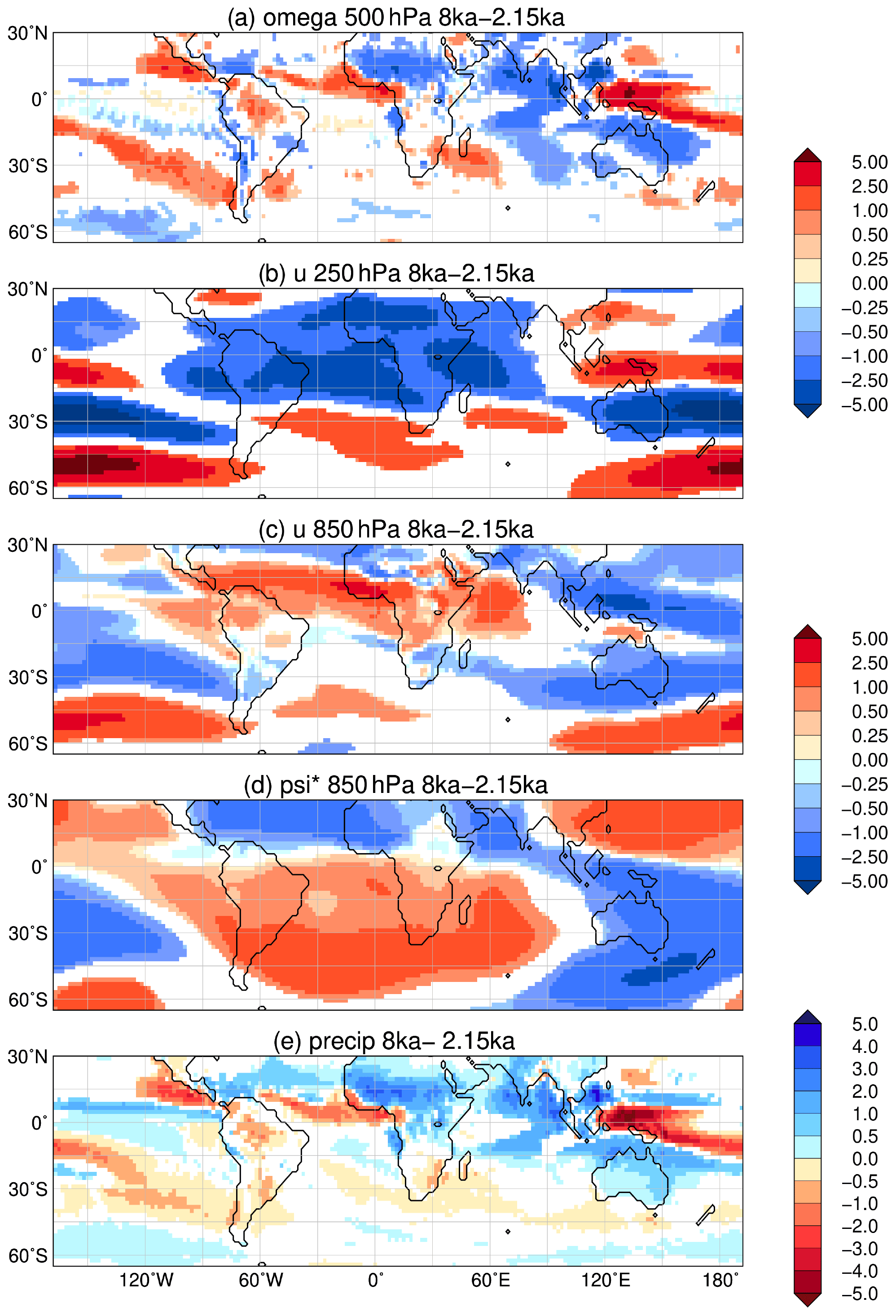
Figure 10Simulated difference in September to November (SON) mean climate in the model for the time slice at 8 ka compared to 2.15 ka, i.e. (a) vertical velocity (omega) in 500 hPa (10−2 m s−1) with blue colour showing increased uplift during 8 ka; (b) upper-tropospheric zonal wind (u) in 250 hPa (m s−1) with blue colours indicating enhanced easterly wind; (c) low-level zonal flow (u) in 850 hPa (m s−1); (d) zonal anomaly in lower-tropospheric streamfunction (psi*, in 107 m2 s−1) reflecting the change in standing waves, with blue colours indicating increased cyclonic circulation at 8 ka compared to 2.15 ka; and (e) mean seasonal precipitation (mm d−1) with blue colours showing enhanced precipitation during 8 ka. Only significant changes are shown (t test, 99 % confidence interval).
The Gran Chaco and Pampas regions east of the South American Andes experience an increase in vegetation during the Holocene, mainly due to an increase in grass cover in the model (Fig. 7). On the southern part of continent, extratropical evergreen trees cover up to 27 % less area at 8 ka compared to 2.15 ka. These vegetation changes are probably related to the increase in both austral wintertime and summertime precipitation during the Holocene. Large parts of the region get precipitation mainly due to the moisture influx in the northeasterly branch of the subtropical Atlantic High. During 8 ka austral winters, this anticyclone is shifted equatorwards, leading to diverging easterly wind anomalies in the lower level and a decrease in moisture flux convergence (not shown). The upper-tropospheric westerly jet is squeezed and intensified along the core (approximately 30∘ S), a pattern that is underlined by Holocene reconstructions (Lamy et al., 2010). The changes in westerlies probably enhance the subsidence in the lee of the Andes. The subsidence is furthermore enhanced by the updraft of the Afro-Asian monsoon that leads to a strong divergence anomaly in the upper-tropospheric velocity potential (Fig. 11) and accordingly to a strong convergence anomaly above South America during austral winter, triggering subsidence. Thus, the change in monsoons is also a key driver of the South American vegetation changes.
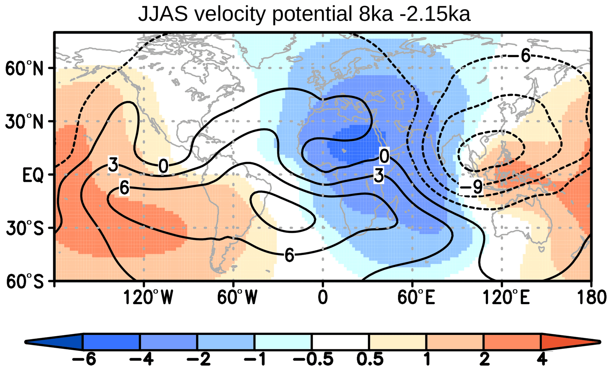
Figure 11Simulated difference (shaded) in June–September mean upper-tropospheric (250 hPa) velocity potential (km2 s−1) between the time slice at 8 ka and 2.15 ka. Bluish colour indicates enhanced divergence, coinciding with vertical ascent in the troposphere below; reddish colour indicates stronger convergence, coinciding with subsidence below. The contours plotted on top show the respective velocity potential at 2.15 ka. Negative values display divergence and positive values convergence.
Figure 5 indicates that the precipitation difference between 8 ka and 2.15 ka in this region is largest during the month November and December. During austral summer, a deep continental low evolves above the South American continent that additionally deflects the easterly winds to the south so that the wind is channelled between the Brazilian Plateau and the Andes. This low-level jet transports huge amounts of moisture southwards at present (Marengo et al., 2004; Garreaud et al., 2009). During mid-Holocene November and December, this low is weakened, in line with the weakened South American monsoon (Fig. 9), whose outflow touches this region at 2.15 ka but not at 8 ka. The model indicate a south wind anomaly in the lower troposphere (i.e. a reduced low-level jet), diminishing the inflow from the monsoon area (not shown).
Overall, the model reveals that vegetation changes south of 60∘ N during the Holocene occur predominantly in monsoon regions, their margins and in extratropical regions that are connected with the monsoons via teleconnections. Thus, our model results point to a strong effect of the monsoon-related changes in atmospheric circulation on the global Holocene vegetation dynamics outside the high northern latitudes. These results confirm earlier findings of monsoon-extratropical teleconnections (e.g. Rodwell and Hoskins, 2001; Gaetani et al., 2011; Nakanishi et al., 2021) and stress the importance of the monsoon system for the global climate and ecosystems. At least during the Holocene, the monsoon systems seemed to be the key player in the climate and vegetation dynamics.
The overview of the patterns of clustered vegetation trends reveals rather linear transitions between different PFT groups during the Holocene (Fig. 2). This appears to be consistent with the assumption that large-scale vegetation change and climate change directly follow the subtle, approximately linear orbital forcing over the last 8000 years. In addition, it agrees with the analysis by Mottl et al. (2021) that reveals a linear, steady change in the vegetation composition between 8 and 4.2 ka before early land use sets in (which is excluded in our simulations in the millennia before 2 ka). However, reconstructions also report of rapid, or abrupt, vegetation changes in different regions of the world. The most prominent example is the expansion of the Sahara from a rather “green Sahara” to its current extent some 5500 years ago. Indicators of regionally (mainly in the western part) rapid changes include the rapid increase in dust deposition found in marine sediments core off the western Sahara coast (e.g. deMenocal et al., 2000). Abrupt regional vegetation changes, at least for individual taxa, are also suggested to exist in central Asia (Zhao et al., 2017), the high northern latitudes (MacDonald et al., 2000), parts of North America (e.g. Marsicek et al., 2013; Shuman et al., 2009; Foster et al., 2006) and Europe (Giesecke et al., 2011; Seddon et al., 2015). How rapid these changes were and whether these changes only reflect local phenomena are still a matter of discussion. Mayewski et al. (2004) identified several phases with rapid global climate changes during the Holocene which might have forced changes in vegetation composition. Ecosystems can respond quite slowly to changes in the local environmental conditions but can also change rapidly when the conditions approach critical thresholds (Scheffer et al., 2001). In addition, initially slow changes can be amplified by feedbacks in the climate system, giving rise to non-linear responses to the orbital forcing (Williams et al., 2002).
The cluster method used to group the globally wide trend in main PFTs in this study is not designed to properly identify rapid changes. The aggregation of the PFTs in the main PFT groups complicates the occurrence of rapid changes as these changes would have to be very extensive and accompanied by very strong climatic changes for an entire PFT group to collapse. Furthermore, the global view masks regionally appearing transitions. To detect non-linearity in the Holocene vegetation change, we suggest evaluating the relative change (R) in the individual PFT fractions (see Appendix C). The change in the individual PFT fraction between two consecutive time steps is compared to the maximum possible change during the period of interest. The noise time series are filtered by a Butterworth filter with a cut-off frequency years. As measure for rapid changes, the maximum Rmax of the absolute value of R is taken.

Figure 12Maximum relative change in PFTs (R) indicating the rapidness of the PFT change. The more yellowish the more rapid is the transition. The model reveals six different regions with rapid changes (regions 1–6).
Figure 12 shows the global patterns of Rmax for the individual PFTs. In total, six regions can be identified that indicate rapid changes in PFT cover fractions, i.e. shifts that exceed the linear trend by a factor of up to 5, given the low-pass filter of 500 years. These regions include areas in the high northern latitudes and the monsoon margins in each hemisphere. The areas coincide with regions where the cluster method also shows relatively strong changes, except for the region of South America in which the rapid changes occur within the forest PFTs.
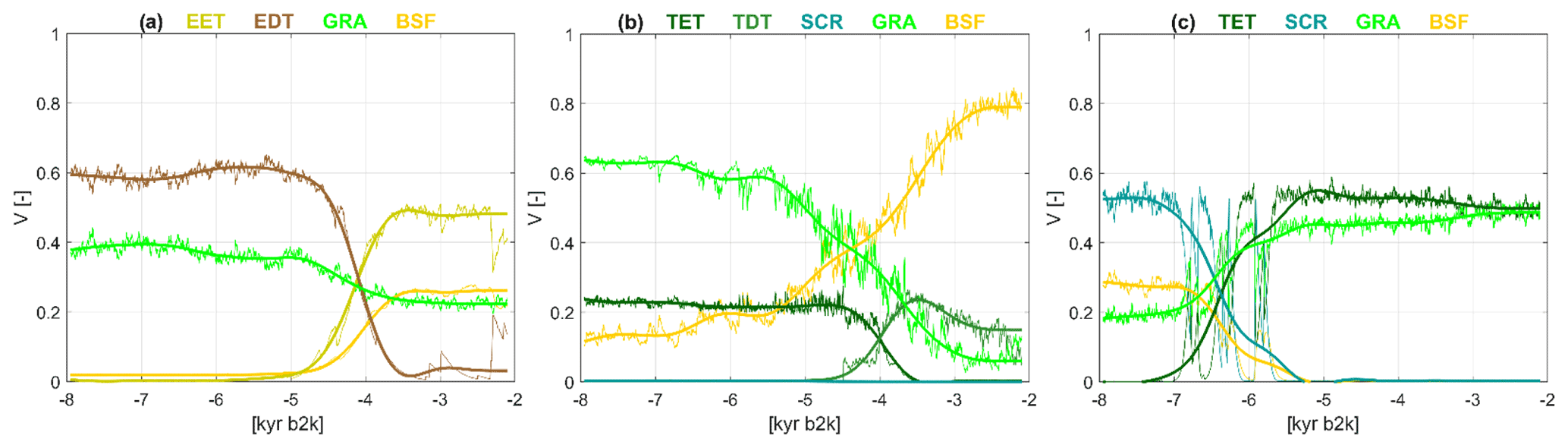
Figure 13Examples of rapid transitions between simulated PFTs in a grid cell in (a) East Siberia (at the grid cell centred at 62.49∘ N, 120∘ E, in region 2 in Fig. 12), (b) today's Sahara–Sahel region (at 19.59∘ N, 7.5∘ W, in region 3) and (c) South Asia (at 19.59∘ N, 78.75∘ E, in region 4), shown as fractional coverage V(t) as function of time t, given as kyr b2k. The colours refer to different PFTs as indicated in the title line. EET: extratropical evergreen trees; EDT: extratropical deciduous trees; TET: tropical evergreen trees; TDT: tropical deciduous trees; SCR: shrubs; GRA: grass; BSF: bare soil fraction. The thin lines are annual values of fractional vegetation coverage, and the thick lines are filtered time series using a Butterworth filter of the order of 5 with a low-pass filter of 500 years.
In northern Canada and eastern Siberia (region 1 and 2), rapid shifts mainly occur between the extratropical deciduous trees and extratropical evergreen trees and, to a weaker extent, in the bare soil fraction. The main processes for the transition are the same as discussed above in Sect. 5.4. A typical example of such a transition in region 1 and 2 is depicted in Fig. 13a for a grid box in eastern Siberia. During the first millennia, extratropical evergreen trees cannot exist, because the temperature of the coldest month is too low. This bioclimatic limit mimics the dependence of extratropical trees on moisture in the high latitudes, because there are no moisture-related bioclimatic thresholds defined in JSBACH. In a very cold, and thus dry, climate, the deciduous trees have an advantage over evergreen trees. Extratropical evergreen trees and extratropical deciduous trees can coexist after about 6 ka. The timescale of the transition from around 6 to some 3.5 ka is governed by the small difference in NPP between the tree PFTs. During the last millennium, rapid fluctuations within a few decades between extratropical evergreen and deciduous trees are found in the simulations. These are induced by fluctuations in the temperature of the coldest month, which may fall below the bioclimatic limit at which extratropical evergreen trees can exist in some years. The extratropical evergreen trees decay within a few decades, and this decay is governed by the timescale of mortality of 50 years prescribed in JSBACH. The extratropical evergreen trees eventually recover at a slower pace which follows the difference in NPP development and which is not explicitly determined by the timescales prescribed in JSBACH.
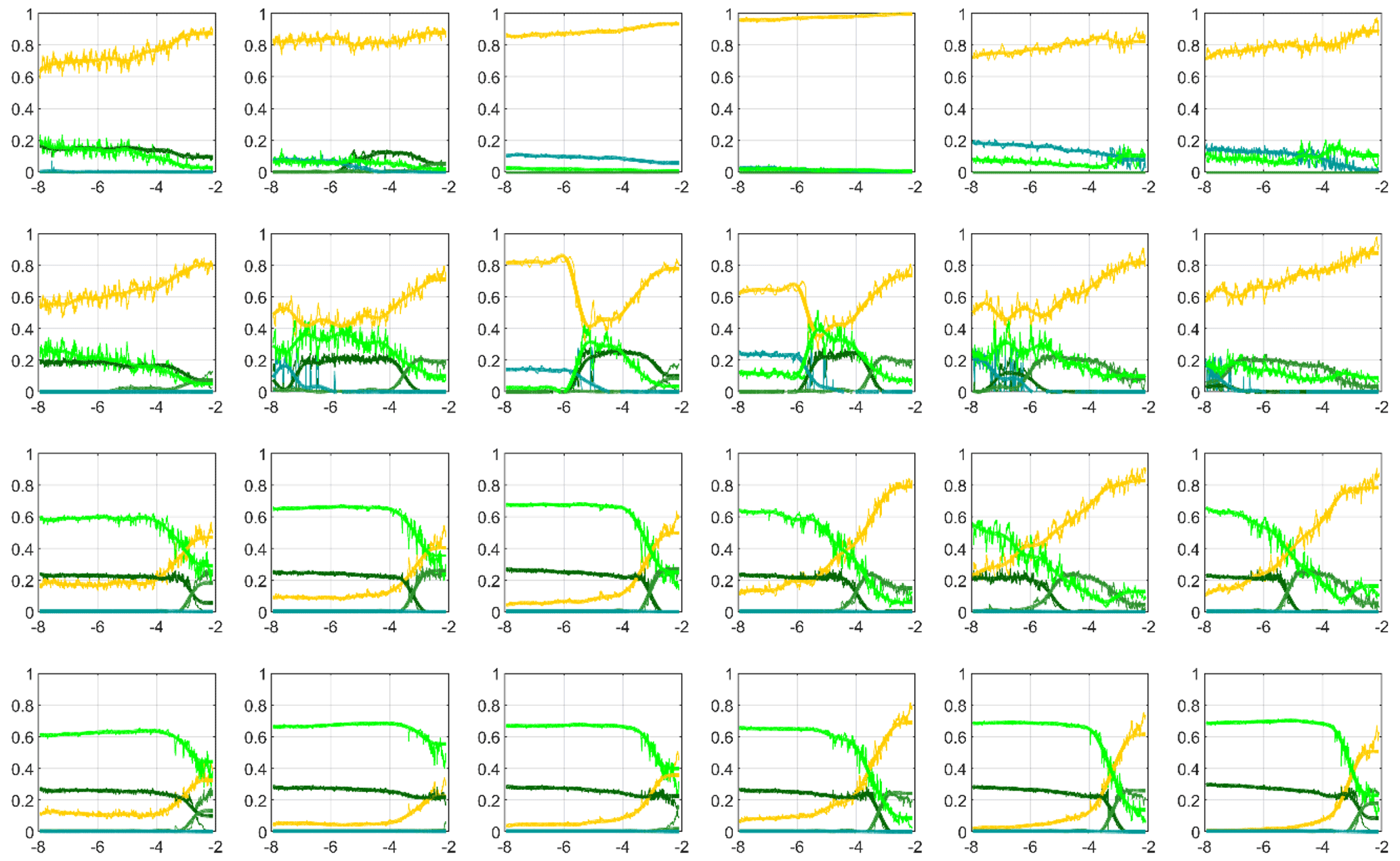
Figure 14Simulated changes in PFTs in the today Sahara–Sahel region (part of region 3 in Fig. 12). The box in the upper left corner is centred at 25.18∘ N, 15∘ W, and the box in the lower right corner is at 19.59∘ N, 5.63∘ W. Like in Fig. 13, the fractional coverage V of PFTs in each grid cell is depicted as function of time, given as kyr b2k. The colours refer to bare soil fraction (yellow), grass (light green), tropical evergreen trees (dark green), tropical deciduous trees (green) and shrubs (blue).
In the Sahel–Sahara transition zone (region 3), the model reveals rapid changes which are also found in some, but not all, pollen records (e.g. Kröpelin et al., 2008; Shanahan et al., 2015) or in Saharan dust transport (e.g. deMenocal et al., 2000). The latter change can directly be linked to rapid landscape changes mainly in the western part of the Sahara (Egerer et al., 2016). The simulated bare soil fraction rapidly increases at the expense of grass cover and, to a much lesser extent, of raingreen shrubs (see Figs. 12 and 14, which provides a zoom into the region 19.59–25.18∘ N and 15.0–5.63∘ W). Bioclimatic limits affect the vegetation change only in the appearance of tropical tree types. Because early mid-Holocene insolation in the tropics is lower than today during winter, the simulated temperature of the coldest month falls below 15.5 ∘C at the beginning of the simulation. This temperature threshold represents the bioclimatic limit for frost-free climate, which is the prerequisite for the existence of tropical trees. During the Holocene, the winter temperature increases, and tropical trees emerge as seen in the in the grid cells centred at the latitude of 25.18∘ N (the first row of grid cells in Fig. 14) and east of 13.13∘ W (the second grid cell from the left in the first row of grid cells). The rapid transition between simulated tropical evergreen trees and tropical deciduous trees seen in some grid cells (e.g. Fig. 13b representing the grid cell centred at 19.59∘ N, 7.5∘ W) is not triggered by crossing a bioclimatic limit. The plant functional types “tropical evergreen tree” and “tropical deciduous tree” have the same temperature requirement in our model. They differ, however, in the parameter values implicit in the rate of carbon fixation computed for the photosynthesis. Therefore, it is the difference in NPP which governs the transition between these PFTs. This transition can be interpreted as a non-linear response to the steady decline in moisture level caused by the retreating summer monsoon during the Holocene, and it generally takes several centuries in our simulations. Similar is valid for the transition between grass and bare soil fraction. Also in this case, it is the decrease in NPP which leads to an increase in bare soil fraction. The simulated shift between tropical tree PFTs appears to be more rapid than the shift between grass and bare soil. The amplitude of the shift in tropical tree cover is, however, much smaller than the decrease in grass and increase in bare soil fraction. A more detailed discussion of simulated and reconstructed vegetation changes in the Sahara–Sahel region is in preparation for a subsequent study.
In South Asia and parts of southeast Asia (region 4), various combinations of rapid changes are found in the simulation. In South Asia, raingreen shrubs decrease rapidly and are replaced by tropical evergreen trees and grasses. As an example, the vegetation dynamics of one grid cell from this region are depicted in Fig. 13b. The transition between the different PFTs is discussed in Sect. 5.1. As in the high northern latitudes, the pace of the transition during the mid-Holocene is governed by the differences in NPP of the PFTs involved. The timescales of allocation and mortality of the competing PFTs differ. They range from 30 years for tropical trees to 12 years for raingreen shrubs. The bioclimatic limit which restricts the occurrence of tropical trees is imposed by the temperature of the coldest month (see Sect. 5.1). In the time period from around 7 to 5.5 ka, this limit is frequently crossed. Because the timescales of allocation and mortality are shorter than those of the PFTs at high northern latitudes, the change between PFTs appears to be more rapid, and the amplitude is larger.
The climatic changes that drive the rapid swings in PFTs in the South American region (region 5) and in the southern African region (region 6) are discussed in Sect. 5.2. The governing timescales of PFT dynamics and the bioclimatic limits involved are the same as those for tropical Asia (region 4).
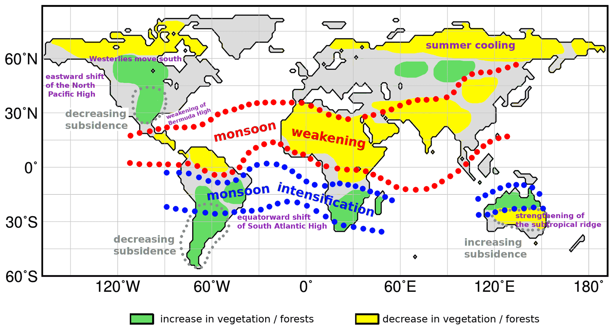
Figure 15Summarizing sketch of the main vegetation, climate and circulation changes from 8 ka to 2.15 ka. South of 60∘ N, the vegetation trend positively correlates with the precipitation trend, i.e. regions with an increasing vegetation and/or forest fraction during the Holocene experienced increasing precipitation, and vice versa for regions with decreasing trend.
Using a cluster analysis technique on a Holocene simulation for the period 8 ka to 2.15 ka with MPI-ESM, the main global natural vegetation trends during the Holocene are identified and discussed in the context of the climate change over the Holocene. A redundancy analysis reveals that precipitation is the main climatic driver leading to regional differences in the vegetation change outside the high northern latitudes. The model is well in line with the overall trends reported by pollen-based vegetation reconstructions. These main trends and their atmospheric drivers in the model are summarized in Fig. 15. They include the following:
- a.
The southward retreat of the tundra and northern treeline by up to 3∘ in latitude, expressed by a bipolar change pattern for all PFT groups with a decrease on the northern site and an increase further south. Asia has been facing the major change in the model by a reduction of the boreal tree cover by nearly one-third since the early mid-Holocene. This transition is mainly related to the seasonal temperature trend driven by the change in insolation during the Holocene. Boreal winter temperatures rise and summer temperatures decline, reducing the growing season and stressing the vegetation in the high northern latitudes. In the polar regions, climate becomes even too harsh for vegetation to survive.
- b.
A decrease and equatorward retreat of all vegetation types in the northern hemispheric monsoon regions, leading to an increase in the deserts, particularly to a vast expansion of the Sahara. The mean non-vegetated area in north Africa north of 15∘ N increases by 22 % during the Holocene, ranging up to 82 % in southern Niger. The reduction in vegetation coincides with the equatorward retreat and the weakening of the northern hemispheric monsoon belts. Our model indicates a decrease of the continental northern hemispheric monsoon area by approximately 25 % since 8 ka. The precipitation in the monsoon regions decreases by approximately 40 % over land, leading to limited moisture availability in large regions.
- c.
An increase in the forest and partly the grass fraction in extratropical North America, leading to an overall increase in vegetated area over the Holocene, forced by a rising moisture level. From the model simulation, we find several possible mechanisms triggering the Holocene increase in precipitation in North America. The North Pacific High is shifted westward and the westerly jet and the related storm tracks are shifted northward during the mid-Holocene, leading to less moisture transport to Canada and the northern Great Plains and enhanced subsidence in large parts of the region. The Bermuda High is slightly strengthened during 8 ka summer, rerouting the moisture transport along the coast and reducing the moisture flux convergence over the Great Plains. Additionally, the strengthening of the ascent in the North American summer monsoon is probably responsible for enhanced subsidence in the Great Plains at 8 ka.
- d.
A small increase in vegetation in the southern hemispheric monsoon regions, induced by an increase in forest, grass and shrubs (southern Africa). Due to the decreased austral summer insolation during the mid-Holocene, the southern hemispheric monsoon systems are weaker at 8 ka compared to 2.15 ka. The continental monsoon domain is reduced by 5 % and the precipitation is decreased by 11 %. Hence, the change in the monsoon strength is weaker than for the Northern Hemisphere. This is also reflected in the relatively minor changes in total vegetation cover. Instead, the southern hemispheric monsoon regions experiences (strong) shifts in the woody PFT composition. The warmer winter climate during the mid-Holocene allows for the establishment of tropical evergreen trees in the model. In the course of the gradual cooling during the Holocene, winter temperatures at some point fall outside the tolerance range of tropical trees, which give way for other woody PFTs. Under the relatively humid conditions in South America, extratropical trees win this competition. In southern Africa, where the moisture is more limited, evergreen trees are replaced by raingreen shrubs. Australia experiences both an increase in extratropical trees (mainly at the east coast) and in raingreen shrubs.
- e.
An increase in the bare soil fraction in extra-monsoonal Australia and an increase in grass and total vegetation in extra-monsoonal South America. Mid-Holocene Australian climate (south of 22∘ S) is slightly wetter than that at 2.15 ka due to a weaker subtropical ridge, less subsidence and a stronger moisture influx from the Pacific Ocean. During the Holocene, precipitation declines, leading to a decrease of the grass cover and extratropical trees that can not be overcompensated by the establishing raingreen shrubs. In South America, austral wintertime precipitation is decreased during the mid-Holocene due to increased subsidence and a decreased moisture flux convergence caused by the poleward-shifted South Atlantic subtropical high. At least partly, the stronger subsidence is related to a remote response to the enhanced north African summer monsoon. In addition, austral summer precipitation is decreased, probably due to a weaker influence of the South American monsoon, upstream of the main lower-tropospheric wind field. The increase in rainfall during the Holocene leads to an increase in grass cover (Gran Chaco and Pampas region) and extratropical evergreen trees (eastern Argentina).
At large scales, the global shifts in vegetation appear to follow the slow, to first order linear, orbital forcing. In some regions, however, the model simulates rapid, strongly non-linear changes in PFTs. These regions include two domains in the high northern latitudes (Canada and central Siberia) and four regions in the monsoon margin area on both hemispheres (Sahel–Sahara, India and southeast Asia, South America and southern Africa). The rapid change in bare soil fraction in the Sahara region can be attributed to the non-linear response of the monsoon precipitation and vegetation to the orbital forcing (cf. Dallmeyer et al., 2020).
Transitions between individual PFTs triggered by changes in climate appear on a large spectrum of timescales. The transitions are governed by the difference in NPP of the competing PFTs. If the PFTs have the same timescales of allocation and mortality, then transitions can take place over many centuries. More rapid transitions in PFTs can occur within a few decades or less, if the climate moves in or out the bioclimatic tolerance so that some temperature thresholds in the model are suddenly met or not fulfilled any more. These rapid changes in simulated vegetation pattern have to be interpreted with care. Bioclimatic limits are known to exist for plant species. Whether the concept of bioclimatic limits can be applied to the temporal dynamics of PFTs has to be critically reassessed. PFTs encompass a variety of different and diverse plant species. Because of this plant diversity within a PFT, PFTs presumably show a larger resilience to climate changes than individual species do. Hence, our model results should be taken as an indicator of possible rapid changes in the vegetation rather than a precise prediction of rapid changes themselves.
This study explores the Holocene vegetation changes around the world and interprets them in terms of the Holocene climate change. The model results reveal that most of the Holocene vegetation trends seen outside the high northern latitudes can be attributed to modifications in the intensity of the global summer monsoons. Due to the seasonal changes in insolation, the monsoon systems in the Northern Hemisphere weaken, while the monsoon systems in the Southern Hemisphere intensify during the Holocene. Due to teleconnections (Rodwell–Hoskins response to the diabatic heating), the intensity change of the monsoons affect the subtropical anticyclones, whose modification in turn leads to an adjustment of the wind field over the extratropical continents. In addition, the magnitude of the updrafts in the monsoon belts determines the strength of the subsidence in the extra-monsoonal areas, such that a weakening of the monsoon rainfall coinciding ascent also weakens the descent abroad. The model results thus identify the global monsoon system as the key player in Holocene climate and vegetation history and point to a far greater importance of the monsoon systems on the extra-monsoonal vegetation dynamics than previously assumed. The model results indicate that changes in the global monsoon dynamic should always be considered as an actor in past and future climate changes, even in regions not primarily influenced by monsoons.
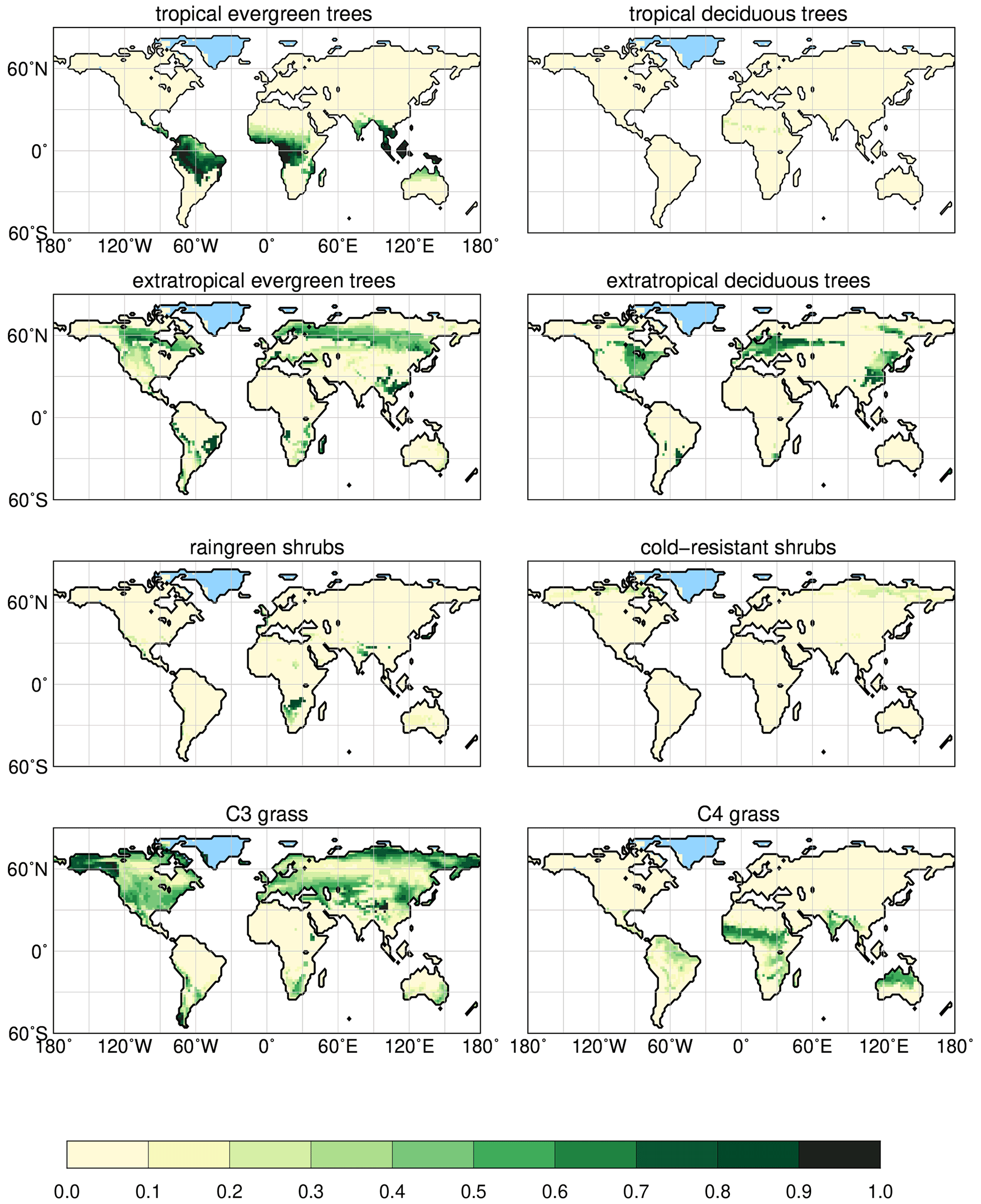
Figure A1Simulated plant functional type distributions at 2.15 ka.
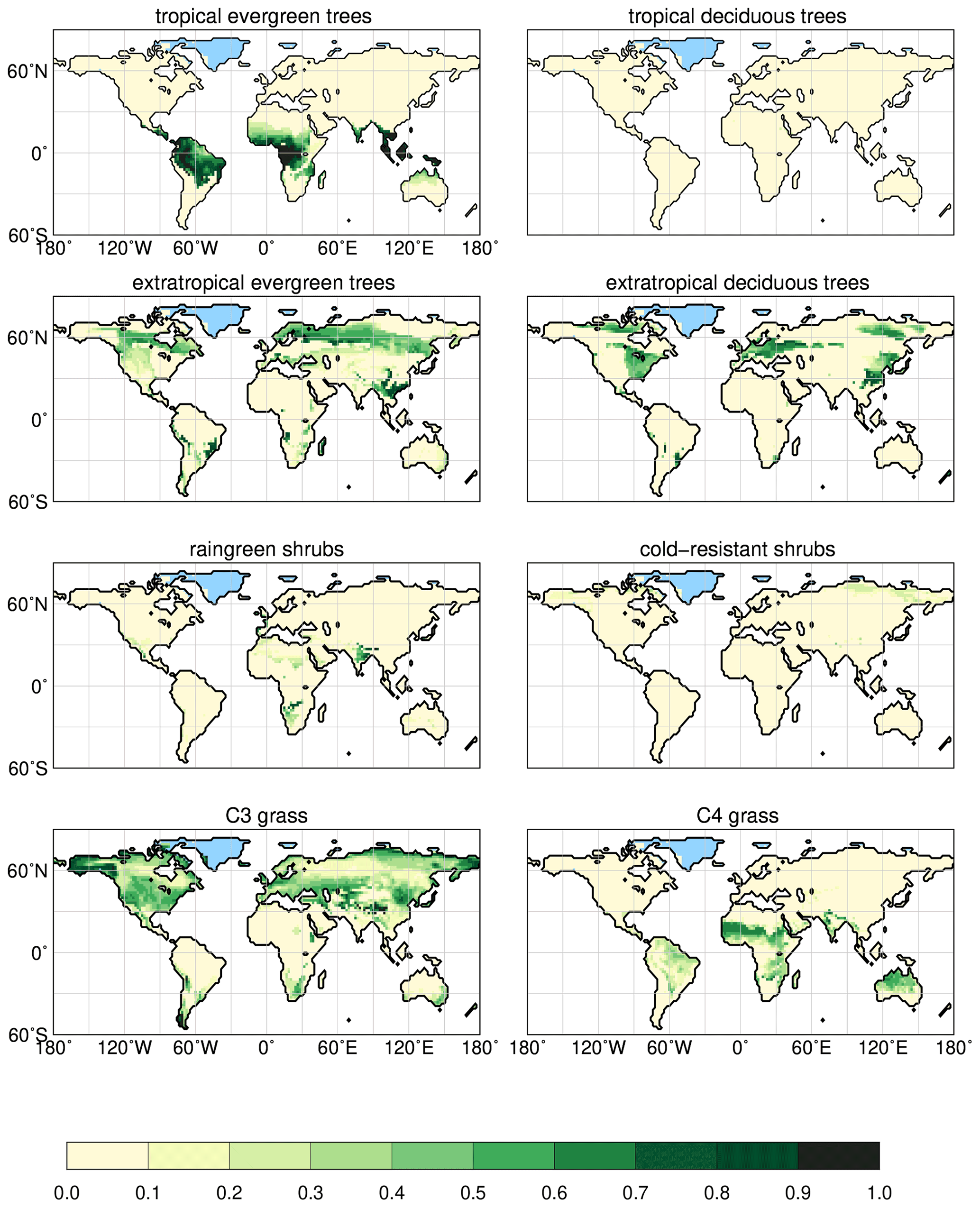
Figure A2Simulated plant functional type distributions at 8 ka.

Figure B1Simulated annual mean sea surface temperatures (SSTs) (K) for (a) the 2.15 ka time slice and (b) the difference between 8 ka and 2.15 ka.
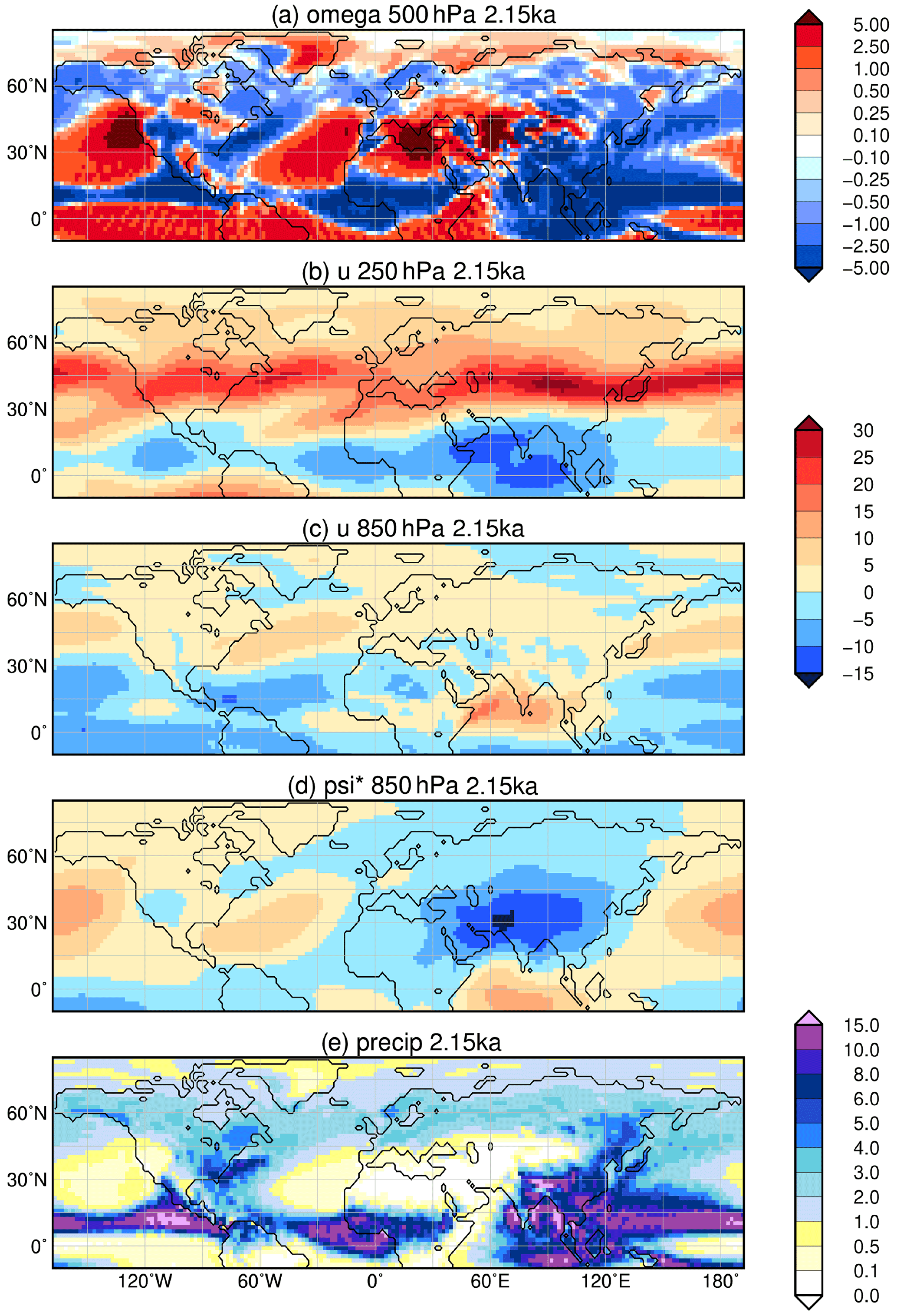
Figure B2Simulated JJA mean climate at 2.15 ka, i.e. (a) vertical velocity (omega) in 500 hPa (10−2 m s−1) with blue colour showing uplift; (b) upper-tropospheric zonal wind (u) in 250 hPa (m s−1) with blue colours indicating easterly wind; (c) low-level zonal flow (u) in 850 hPa (m s−1); (d) zonal anomaly in lower-tropospheric streamfunction (psi*, in 107 m2 s−1) reflecting the standing waves, with blue colours indicating cyclonic circulation; and (e) mean seasonal precipitation (mm d−1).
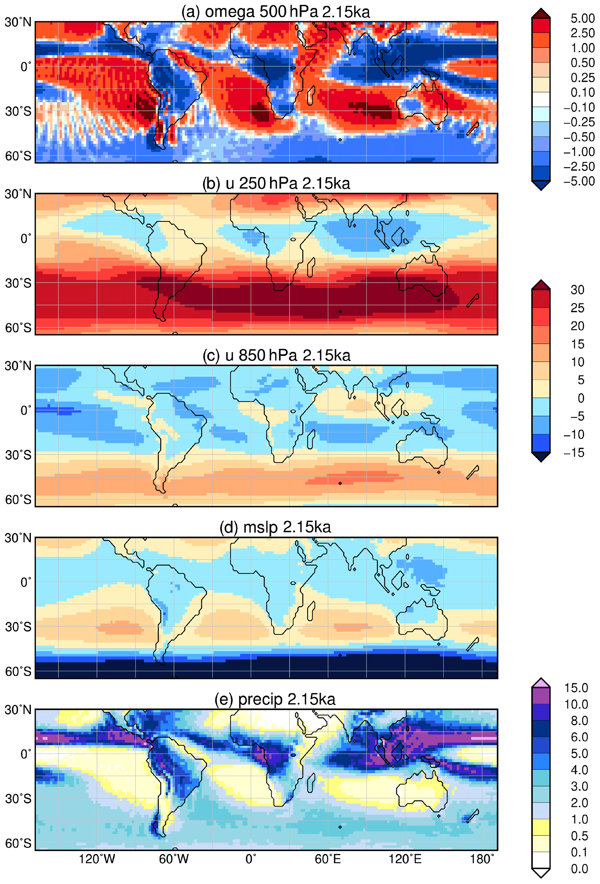
Figure B3Simulated SON mean climate at 2.15 ka, i.e. (a) vertical velocity (omega) in 500 hPa (10−2 m s−1) with blue colour showing uplift; (b) upper-tropospheric zonal wind (u) in 250 hPa (m s−1) with blue colours indicating easterly wind; (c) low-level zonal flow (u) in 850 hPa (m s−1); (d) mean sea level pressure anomaly (hPa) to standard atmospheric mean pressure (here 1013.25 hPa), with blue colours indicating low-pressure systems; and (e) mean seasonal precipitation (mm d−1).
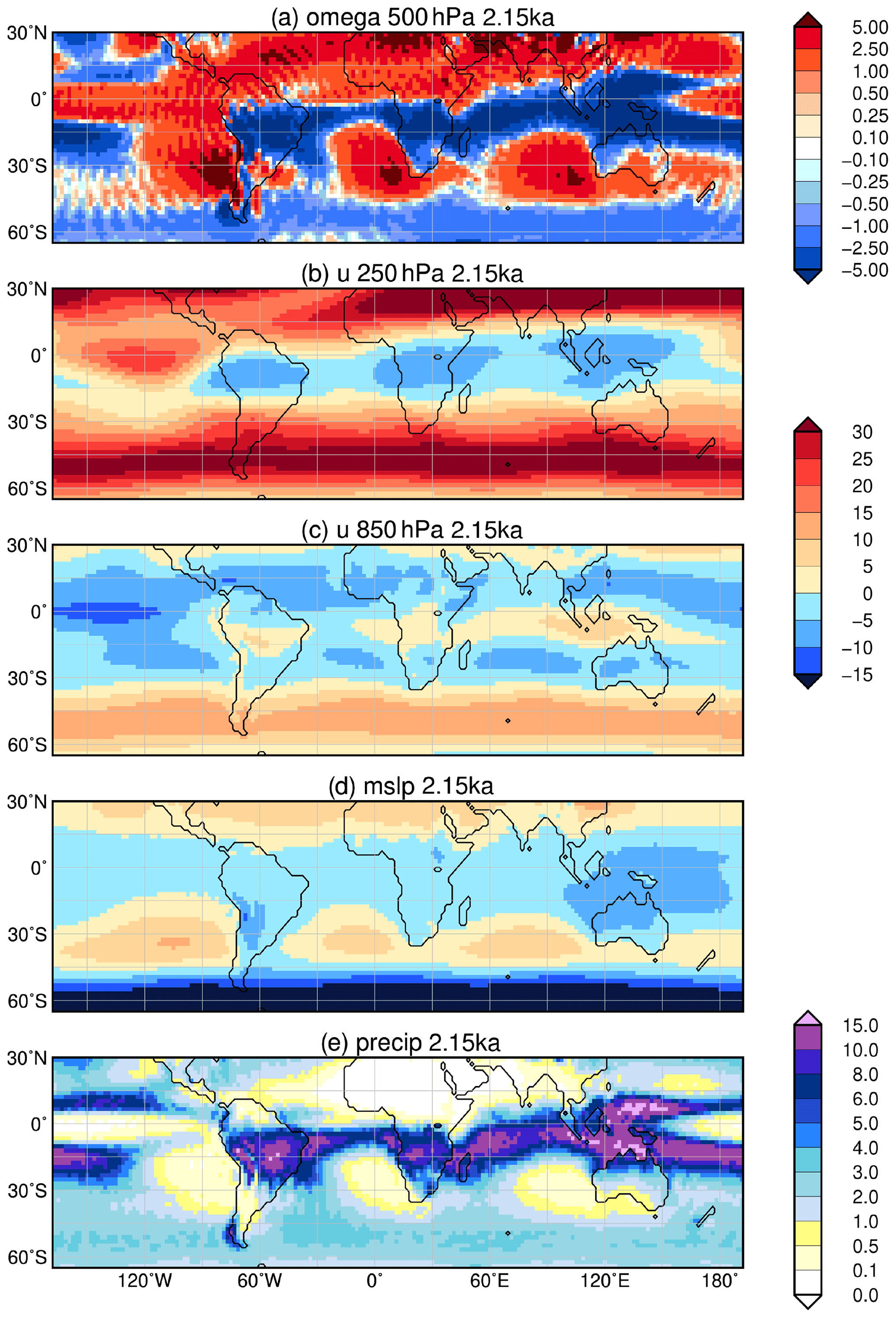
Figure B4Simulated DJF mean climate at 2.15 ka, i.e. (a) vertical velocity (omega) in 500 hPa (10−2 m s−1) with blue colour showing uplift; (b) upper-tropospheric zonal wind (u) in 250 hPa (m s−1) with blue colours indicating easterly wind; (c) low-level zonal flow (u) in 850 hPa (m s−1); (d) mean sea level pressure anomaly (hPa) to standard atmospheric mean pressure (here 1013.25 hPa), with blue colours indicating low-pressure systems; and (e) mean seasonal precipitation (mm d−1).
We evaluate the temporal change of the simulated vegetation fraction V of a PFT relative to an overall amplitude ΔV and over the entire period ΔT considered, in our case, ΔT=6000 years. We define the relative change R by
We define the overall amplitude ΔV as the maximum possible change that the vegetation fraction can reach, i.e. ΔV=1, to focus on large and rapid vegetation changes. The simulated vegetation cover V varies on all timescales. Some of these variations can be attributed to fluctuations in climate which affect the net primary productivity (NPP). Variations in V also occur when the bioclimatic limit at which a PFT can exist is crossed. Then V decreases exponentially on timescales of decades and shorter, or it increases abruptly, if colonizable space is available, or the PFT grows at the expense of other PFTs. Examples are given in Fig. 13a and c. This type of abrupt change, which is known to happen at species level, is likely to be a model artefact at biome level. Therefore, we apply a Butterworth filter of the order of 5 to separate very brief fluctuations in simulated vegetation fraction from fluctuations beyond the decadal timescale.
Figure C1 demonstrates the effect of filtering. In Fig. C1, changes in extratropical deciduous trees in a grid box in East Siberia (the same grid box as that shown in Fig. 13a) are depicted. The unfiltered time series reveals small, rapid changes at decadal timescale in the first millennia of the simulation, a large transition around 4 ka, and larger and rapid decadal fluctuations during the last millennia. When applying a Butterworth filter of the order of 5 with a cut-off frequency years, only the large transition around 4 ka is identified as the most rapid change.
Figure 12 shows the maxima of the absolute value of R using years,
hence, we do not differentiate cases of strong increase or decrease in vegetation fraction. Using smaller or larger values of F would result in different values of Rmax, as indicated in the example Fig. C1, but the overall global patterns, specifically the regions of strongest non-linear change shown in Fig. 12, would be more or less the same.

Figure C1Effect of filtering on Rmax. Black lines indicate fractional coverage of extratropical deciduous trees in a grid box in East Siberia centred at 62.48∘ N, 120∘ E, in region 2 (see Figs. 12 and 13a) as function of time (in ka). The thin lines are annual values of fractional vegetation coverage V(t), and the thick lines are filtered time series of V(t) using a Butterworth filter of the order of 5 with a low-pass filter of (a) F of 100 years, (b) F of 250 years, (c) F of 500 years, (d) F of 750 years. The absolute value of the relative change R is shown as a dotted red line. The titles of each subfigure indicate the strength of the low-pass filter F, the maximum of the absolute value of the relative change Rmax and the time t at which Rmax occurs.
The primary data, i.e. the model code for MPI-ESM, are freely available to the scientific community and can be accessed with a license (https://mpimet.mpg.de/en/science/modeling-with-icon/code-availability, last access: 24 November 2021). In addition, secondary data and scripts that may be useful in reproducing the authors' work are archived by the Max Planck Institute for Meteorology and are accessible without any restrictions (http://hdl.handle.net/21.11116/0000-0008-8051-B, MPG.PuRe, 2021).
The Biome6000 pollen-based biome reconstructions that we used for the evaluation of the model can be downloaded from https://doi.org/10.17864/1947.99 (Harrison, 2017).
Volcanic forcing data are available at https://doi.org/10.1594/PANGAEA.928646 (Sigl et al., 2021).
AD and MC wrote the manuscript; SJL ran the simulation; MS and MT provided the volcanic forcing data. MC, UH and AD planned the study and were involved in the analysis. All authors discussed the analysis and the manuscript.
Martin Claussen is editor of Climate of the Past. The peer-review process was guided by an independent editor, and the authors also have no other competing interests to declare.
Publisher's note: Copernicus Publications remains neutral with regard to jurisdictional claims in published maps and institutional affiliations.
This work contributes to the project PalMod, funded by the German Federal Ministry of Education and Research (BMBF), Research for Sustainability initiative (FONA, http://www.fona.de, last access: 24 November 2021). Anne Dallmeyer was financed by PalMod (grant no. 01LP1920A). Michael Sigl acknowledges funding from the European Research Council (ERC) under the European Union's Horizon 2020 research and innovation programme (grant agreement no. 820047). This work also contributes to the project African and Asian Monsoon Margins of the Cluster of Excellence EXC 2037: Climate, Climatic Change, and Society (CLICCS). We thank Thomas Kleinen (MPI-M) for his helpful comments on an earlier version of the manuscript. We acknowledge Joseph R. McConnell, Jihong Cole-Dai and Mirko Severi for providing ice-core data. We would like to thank the editor, Steven Phipps, for kindly handling this paper. We thank the referee Qiong Zhang and the two anonymous referees for their constructive suggestions for improving our manuscript.
This research has been supported by the Bundesministerium für Bildung und Forschung (grant no. 01LP1920A) and the H2020 European Research Council (grant no. 820047).
The article processing charges for this open-access publication were covered by the Max Planck Society.
This paper was edited by Steven Phipps and reviewed by Qiong Zhang and two anonymous referees.
Bader, J., Jungclaus, J., Krivova, N., Lorenz, S., Maycock, A., Raddatz, T., Schmidt, H., Toohey, M., Wu, C.-J, and Claussen, M.: Global temperature modes shed light on the Holocene temperature conundrum, Nat. Commun., 11, 4726, https://doi.org/10.1038/s41467-020-18478-6, 2020.
Barr, C., Tibby, J., Leng, M. J., Tyler, J. J., Henderson, A. C. G., Overpeck, J. T., Simpson, G. L., Cole, J. E., Phipps, S. J., Marshall, J. C., Mcgregor, G. B., Hua, Q., and Mcrobie, F. H.: Holocene El Niño–Southern Oscillation variability reflected in subtropical Australian precipitation, Sci. Rep., 9, 1627, https://doi.org/10.1038/s41598-019-38626-3, 2019.
Bartlein, P. J. and Shafer, S. L.: Paleo calendar-effect adjustments in time-slice and transient climate-model simulations (PaleoCalAdjust v1.0): impact and strategies for data analysis, Geosci. Model Dev., 12, 3889–3913, https://doi.org/10.5194/gmd-12-3889-2019, 2019.
Behling, H. and Hooghiemstra, H.: Neotropical savanna environments in space and time: Late Quaternary interhemispheric comparisons, chap. 18, in: Interhemispheric Climate Linkages, edited by: Markgraf, V., Academic Press, San Diego, USA, 2001.
Berger, A. L.: Long-term variations of daily insolation and quater-nary climatic changes, J. Atmos. Sci., 35, 2362–2367, 1978.
Bezdek, J. C.: Pattern Recognition with Fuzzy Objective Function Al-gorithms, Plenum, New York, USA, 1981.
Bigelow, N. H., Brubaker, L. B., Edwards, M. E., Harrison, S. P., Prentice, I. C., Anderson, P. M., Andreev, A. A., Bartlein, P. J., Christensen, T. R., Cramer, W., Kaplan, J. O., Lozhkin, A. V., Matveyeva, N. V., Murray, D. F., McGuire, A. D., Razzhivin, V. Y., Ritchie, J. C., Smith, B., Walker, D. A., Gajewski, K., Wolf, V., Holmqvist, B. H., Igarashi, Y., Kremenetskii, K., Paus, A., Pisaric, M. F. J., and Volkova, V. S.: Climate change and Arctic ecosystems: 1. Vegetation changes north of 55 degrees N between the last glacial maximum, mid-Holocene, and present, J. Geophys. Res.-Atmos., 108, 8170, https://doi.org/10.1029/2002JD002558, 2003.
Bond, W. J.: What limits trees in C4 grasslands and savannas?, Annu. Rev. Ecol. Evol. Syst., 39, 641–659, https://doi.org/10.1146/annurev.ecolsys.39.110707.173411, 2008.
Bond, W. J., Midgley, G. F., and Woodward, F. I.: What controls South African vegetation-climate or fire?, S. Afr. J. Bot., 69, 79–91, 2003.
Braconnot, P., Zhu, D., Marti, O., and Servonnat, J.: Strengths and challenges for transient Mid- to Late Holocene simulations with dynamical vegetation, Clim. Past, 15, 997–1024, https://doi.org/10.5194/cp-15-997-2019, 2019.
Brovkin, V., Bendtsen, J., Claussen, M., Ganopolski, A., Kubatzki, C., Petoukhov, V., and Andreev, A.: Carbon cycle, vegetation, and climate dynamics in the Holocene: Experiments with the CLIMBER-2 model, Global Biogeochem. Cy., 16, 1139, https://doi.org/10.1029/2001GB001662, 2002.
Brovkin, V., Raddatz, T., Reick, C. H., Claussen, M., and Gayler, V.: Global biogeophysical interactions between forest and climate. Geophys. Res. Lett., 36, L07405, https://doi.org/10.1029/2009GL037543, 2009.
Brovkin, V., Lorenz, S., Raddatz, T., Ilyina, T., Stemmler, I., Toohey, M., and Claussen, M.: What was the source of the atmospheric CO2 increase during the Holocene?, Biogeosciences, 16, 2543–2555, https://doi.org/10.5194/bg-16-2543-2019, 2019.
Burrough, S. L. and Thomas, D. S. G.: Central southern Africa at the time of the African Humid Period: a new analysis of Holocene palaeoenvironmental and palaeoclimate data, Quaternary Sci. Rev., 80, 29–46, https://doi.org/10.1016/j.quascirev.2013.08.001, 2013.
Cao, X., Tian, F., Dallmeyer, A., and Herzschuh, U.: Northern Hemisphere biome changes (> 30∘ N) since 40 cal ka BP and their driving factors inferred from model-data comparisons, Quaternary Sci. Rev., 220, 291–309, https://doi.org/10.1016/j.quascirev.2019.07.034, 2019a.
Cao, X., Tian, F., Li, F., Gaillard, M.-J., Rudaya, N., Xu, Q., and Herzschuh, U.: Pollen-based quantitative land-cover reconstruction for northern Asia covering the last 40 ka cal BP, Clim. Past, 15, 1503–1536, https://doi.org/10.5194/cp-15-1503-2019, 2019b.
Chauhan, M. S., Sharma, A., Phartiyal, B., and Kumar, K.: Holocene vegetation and climatic variations in Central India: A study based on multiproxy evidences, J. Asian Earth Sci., 77, 45–58, https://doi.org/10.1016/j.jseaes.2013.08.005, 2013.
Clement, A. C., Hall, A., and Broccoli, A.: The importance of precessional signals inthe tropical climate, Clim. Dynam., 22, 327–341, 2004.
Cole-Dai, J., Ferris, D. G., Kennedy, J. A., Sigl, M., McConnell, J. R., Fudge, T. J., Geng, L., Maselli, O. J., Taylor, K. C., and Souney, J. M.: Comprehensive record of volcanic eruptions in the Holocene (11 000 years) from the WAIS Divide, Antarctica ice core, J. Geophys. Res.-Atmos., 126, e2020JD032855, https://doi.org/10.1029/2020JD032855, 2021.
Crowley, T. J. and Unterman, M. B.: Technical details concerning development of a 1200 yr proxy index for global volcanism, Earth Syst. Sci. Data, 5, 187–197, https://doi.org/10.5194/essd-5-187-2013, 2013.
Crucifix, M., Loutre, M. F, Tulkens, P., Fichefet, T., and Berger, A.: Climate evolution during the Holocene: A study with an Earth system model of intermediate complexity, Clim. Dynam., 19, 43–60, 10.1007/S00382-001-0208-6, 2002.
Cruz, F. W., Vuille, M., and Burns, S. J.: Orbitally driven east–west antiphasing of South American precipitation, Nat. Geosci., 2, 210–214, 2009.
D'Agostino, R., Bader, J., Bordoni, S., Ferreira, D., and Jungclaus, J: Northern hemisphere monsoon response to mid-holocene orbital forcing and greenhouse gas-induced global warming, Geophys. Res. Lett., 46, 1591–1601, 2019.
Dallmeyer, A., Claussen, M., Fischer, N., Haberkorn, K., Wagner, S., Pfeiffer, M., Jin, L., Khon, V., Wang, Y., and Herzschuh, U.: The evolution of sub-monsoon systems in the Afro-Asian monsoon region during the Holocene– comparison of different transient climate model simulations, Clim. Past, 11, 305–326, https://doi.org/10.5194/cp-11-305-2015, 2015.
Dallmeyer, A., Claussen, M., and Brovkin, V.: Harmonising plant functional type distributions for evaluating Earth system models, Clim. Past, 15, 335–366, https://doi.org/10.5194/cp-15-335-2019, 2019.
Dallmeyer, A., Claussen, M., Lorenz, S. J., and Shanahan, T.: The end of the African humid period as seen by a transient comprehensive Earth system model simulation of the last 8000 years, Clim. Past, 16, 117–140, https://doi.org/10.5194/cp-16-117-2020, 2020.
Davis, B. A. S., Brewer, S., Stevenson, A. C., and Guiot, J.: The temperature of Europe during the Holocene reconstructed from pollen data, Quaternary Sci. Rev. 22, 1701–1716, 2003.
deMenocal, P. B., Ortiz, J., Guilderson, T., Adkins, J., Santhein, M., Baker, L., and Yarusinsky, M.: Abrupt onset and termination of the African Humid Period: Rapid climate responses to gradual insolation forcing, Quaternary Sci. Rev., 19, 347–361, 2000.
Egerer, S., Claussen, M., Reick, C., and Stanelle, T.: The link between marine sediment records and changes in Holocene Saharan landscape: simulating the dust cycle, Clim. Past, 12, 1009–1027, https://doi.org/10.5194/cp-12-1009-2016, 2016.
Feng, Z.-D., An, C. B., and Wang, H. B.: Holocene climatic and environmental changes in the arid and semi-arid areas of China: a review, Holocene, 16, 119–130, 2006.
Fischer, N. and Jungclaus, J. H.: Evolution of the seasonal temperature cycle in a transient Holocene simulation: orbital forcing and sea-ice, Clim. Past, 7, 1139–1148, https://doi.org/10.5194/cp-7-1139-2011, 2011.
Fletcher, M. S. and Moreno, P. I.: Have the Southern Westerlies changed in a zonally symmetric manner over the last 14 000 years? A hemisphere-wide take on a controversial problem, Quatern. Int., 253, 32-46, https://doi.org/10.1016/j.quaint.2011.04.042, 2012.
Foster, D. R., Oswald, W. W., Faison, E. K., Doughty, E. D., and Hansen, B. C. S.: A climatic driver for abrupt mid-Holocene vegetation dynamics and the hemlock decline in New England, Ecology, 87, 2959–2966, 2006.
Gaetani, M., Pohl, B., Douville, H., and Fontaine, B.: West African Monsoon influence on the summer Euro-Atlantic circulation, Geophys. Res. Lett., 38, 38–42, https://doi.org/10.1029/2011GL047150, 2011.
Gao, C. C., Oman, L., Robock, A., and Stenchikov, G. L.: Atmospheric volcanic loading derived from bipolar ice cores: Accounting for the spatial distribution of volcanic deposition, J. Geophys. Res.-Atmos., 112, D09109, https://doi.org/10.1029/2006JD007461, 2007.
Garreaud, R. D., Vuille, M., Compagnucci, R., and Marengo, J.: Present-day South American climate. Palaeogeogr. Palaeocl., 281, 180–195, 2009.
Giesecke, T., Bennett, K. D., Birks, H. J. B., Bjune, A. E., Bozilova, E., Feurdean, A., Finsinger, W., Froyd, C., Pokorny, P., Rosch, M., Seppa, H., Tonkov, S., Valsecchi, V., and Wolters, S.: The pace of Holocene vegetation change – testing for synchronous developments, Quaternary Sci. Rev., 30, 2805–2814, https://doi.org/10.1016/j.quascirev.2011.06.014, 2011.
Gill, A. E.: Some simple solutions for heat-induced tropical circulation, Quart. J. Roy. Meteor. Soc., 106, 447–462, 1980.
Grimm, E. C.: Lozano-García, S., Behling, H., Markgraf, V.: Holocene Vegetation and Climate Variability in the Americas, Interhemispheric Climate Linkages, chap. 19, Academic Press, 325–370, https://doi.org/10.1016/B978-012472670-3/50022-7, 2001.
Harrison, S.: BIOME 6000 DB classified plotfile version 1, University of Reading [data set], https://doi.org/10.17864/1947.99, 2017.
Harrison, S. P., Kutzbach, J. E., Liu, Z., Bartlein, P. J., Otto-Bliesner, Muhs, D., Prentice, I. C., and Thompson, R. S.: Mid-Holocene climates of the Americas: A dynamical response to changed seasonality, Clim. Dynam., 20, 663–688, 2003.
Haug, G. H., Hughen, K. A., Sigman, D. M., Peterson, L. C., and Rfhl, U.: Southward migration of the Intertropical Convergence Zone through the Holocene, Science, 293, 1304–1308, 2001.
Hély, C., Lézine, A.-M., and contributors, A.: Holocene changes in African vegetation: tradeoff between climate and water availability, Clim. Past, 10, 681–686, https://doi.org/10.5194/cp-10-681-2014, 2014.
Herzschuh, U., Birks, H. J. B., Ni, J., Zhao, Y., Liu, H., Liu, X., and Grosse, G.: Holocene land-cover changes on the Tibetan Plateau, Holocene, 20, 91–104, 2010.
Hopcroft, P., Valdes, P., Harper, A., and Beerling, D.: Multi vegetation model evaluation of the Green Sahara climate regime, Geophys. Res. Lett., 44, 6804–6813, https://doi.org/10.1002/2017GL073740, 2017.
Hurtt, G. C., Chini, L., Sahajpal, R., Frolking, S., Bodirsky, B. L., Calvin, K., Doelman, J. C., Fisk, J., Fujimori, S., Klein Goldewijk, K., Hasegawa, T., Havlik, P., Heinimann, A., Humpenöder, F., Jungclaus, J., Kaplan, J. O., Kennedy, J., Krisztin, T., Lawrence, D., Lawrence, P., Ma, L., Mertz, O., Pongratz, J., Popp, A., Poulter, B., Riahi, K., Shevliakova, E., Stehfest, E., Thornton, P., Tubiello, F. N., van Vuuren, D. P., and Zhang, X.: Harmonization of global land use change and management for the period 850–2100 (LUH2) for CMIP6, Geosci. Model Dev., 13, 5425–5464, https://doi.org/10.5194/gmd-13-5425-2020, 2020.
Ilyina, T., Six, K., Segschneider, J., Maier-Reimer, E., Li, H., and Núñez-Riboni, I.: Global ocean biogeochemistry model HAMOCC: Model architecture and performance as component of the MPI-Earth System Model in different CMIP5 experimental realizations, J. Adv. Model. Earth Syst., 5, 287–315, https://doi.org/10.1029/2012MS000178, 2013.
Jiang, D., Tian, Z., and Lang, X.: Mid-Holocene global monsoon area and precipitation from PMIP simulations, Clim. Dynam., 44, 2493–2512, https://doi.org/10.1007/s00382-014-2175-8, 2015.
Jolly, D., Prentice, I. C., Bonneille, R., Ballouche, A., Bengo, M., Brenac, P., Buchet, G., Burney, D., Cazet, J.-P., Cheddadi, R., Edorh, T., Elenga, H., Elmoutaki, S., Guiot, J., Laarif, F., Lamb, H., Lezine, A.-M., Maley, J., Mbenza, M., Peyron, O., Reille, M., Reynaud-Farrera, I., Riollet, G., Ritchie, J. C., Roche, E., Scott, L., Ssemmanda, I., Straka, H., Umer, M., Van Campo, E., Vilimumbalo, S., Vincens, A., and Waller, M.: Biome reconstruction from pollen and plant macrofossil data for Africa and the Arabian peninsula at 0 and 6000 years, J. Biogeogr., 25, 1007–1027, 1998.
Jungclaus, J. H., Fischer, N., Haak, H., Lohmann, K., Marotzke, J., Matei, D., Mikolajewicz, U., Notz, D., and von Storch, J. S.: Characteristics of the ocean simulations in the Max Planck Institute Ocean Model (MPIOM) the ocean component of the MPI-Earth system model, J. Adv. Model. Earth Syst., 5, 422–446, https://doi.org/10.1002/jame.20023, 2013.
Köhler, P.: Interactive comment on “What was the source of the atmospheric CO2 increase during the Holocene?” by Victor Brovkin et al., Biogeosciences Discuss., https://doi.org/10.5194/bg-2019-64-SC1, 2019.
Krivova, N. A., Solanki, S. K., and Unruh, Y. C.: Towards a long-term record of solar total and spectral irradiance, J. Atmos. Sol.-Terr. Phy., 73, 223–234, 10.1016/j.jastp.2009.11.013, 2011.
Kröpelin, S., Verschuren, D., Lézine, A.-M., Eggermont, H., Cocquyt, C., Francus, P., Cazet, J.-P., Fagot, M., Rumes, B., Russell, J. M., Darius, F., Conley, D. J., Schuster, M., von Suchodoletz, H., and Engstrom, D. R.: Climate-driven ecosystem succession in the Sahara: the past 6000 years, Science, 320, 765–768, 2008.
Kutzbach, J. E.: Monsoon climate of the early Holocene – climate experiment with the earths orbital parameters for 9000 years ago, Science, 214, 59–61, 1981.
Lamy, F., Hebbeln, D., Röhl, U., and Wefer, G.: Holocene rainfall variability in southern Chile: a marine record of latitudinal shifts of the Southern Westerlies, Earth Planet. Sc. Lett., 185, 369–382, https://doi.org/10.1016/S0012-821X(00)00381-2, 2001.
Lamy, F., Kilian, R., Arz, H. W., Francois, J.-P., Kaiser, J., Prange, M., and Steinke, T.: Holocene changes in the position and intensity of the southern westerly wind belt, Nat. Geosci., 3, 695–699, https://doi.org/10.1038/ngeo959, 2010.
Ledru, M. P., Mourguiart, P., and Riccomini, C.: Related changes in biodiversity, insolation and climate in the Atlantic rainforest since the last interglacial, Palaeogeogr. Palaeocl., 271, 140–152, 2009.
Li, F., Gaillard, M.-J., Cao, X., Herzschuh, U., Sugita, S., Tarasov, P. E., Wagner, M., Xu, Q., Ni, J., Wang, W., Zhao, Y., An, C., Beusen, A. H. W., Chen, F., Feng, Z., Klein Goldewijk, C. G. M., Huang, X., Li, Y., Li, Y., Liu, H., Sun, A., Yao, Y., Zheng, Z., and Jia, X.: Toward quantification of Holocene anthropogenic land-cover change in temperate China: a review in the light of pollen-based REVEALS reconstructions of regional plant cover, Earth-Sci. Rev., 203, 103119, https://doi.org/10.1016/j.earscirev.2020.103119, 2020.
Liu, J., Wang, B., Ding, Q., Kuang, X., Soon, W., and Zorita, E.: Centennial variations of the global monsoon precipitation in the last millennium: Results from ECHO-G model, J. Climate, 22, 2356–2371, https://doi.org/10.1175/2008JCLI2353.1, 2009.
Liu, Z., Otto-Bliesner, B., Kutzbach, J., Li, L., and Shields, C.: Coupled Climate Simulation of the Evolution of Global Monsoons in the Holocene, J. Climate, 16, 2472–2490, https://doi.org/10.1175/1520-0442(2003)016<2472:CCSOTE>2.0.CO;2, 2003.
Liu, Z., Harrison, S. P., Kutzbach, J., and Otto-Bliesner, B.: Global monsoons in the mid-Holocene and oceanic feedback, Clim. Dynam., 22, 157–182, https://doi.org/10.1007/s00382-003-0372-y, 2004.
Lorenz, S. J., Kim, J.-H., Rimbu, N., Schneider, R. R., and Lohmann, G.: Orbitally driven insolation forcing onHolocene climate trends: Evidence from alkenone data and climate modeling, Paleoceanography, 21, PA1002, https://doi.org/10.1029/2005PA001152, 2006.
MacDonald, G. M., Velichko, A. A., Kremenetski, C. V., Borisova, O. K., Goleva, A. A., Andreev, A. A., Cwynar, L. C., Riding, R. T., Forman, S. L., Edwards, T. W. D., Aravena, R., Hammarlund, D., Szeicz, J. M., and Gattaulin, V. N.: Holocene treeline history and climate change across northern Eurasia, Quat. Res., 53, 302–311, 2000.
Maksic, J., Shimizu, M. H., Sampaio, G., Venancio, I. M., Cardoso, M., and Ferreira, F. A.: Simulation of the holocene climate over South America and impacts on the vegetation, Holocene, 29, 287–299, 2019.
Marchant, R., Richer, S., Boles, O., Capitani, C., Courtney-Mustaphi, C. J., Lane, P., Prendergast, M. E., Stump, D., De Cort, G., Kaplan, J. O., Phelps, L., Kay, A., Olago, D., Petek, N., Platts, P. J., Punwong, P., Widgren, M., Wynne-Jones, S., Ferro-Vázquez, C., Benard, J., Boivin, N., Crowther, A., Cuní-Sanchez, A., Deere, N. J., Ekblom, A., Farmer, J., Finch, J., Fuller, D., Gaillard-Lemdahl, M.-J., Gillson, L., Githumbi, E., Kabora, T., Kariuki, R., Kinyanjui, R., Kyazike, E., Lang, C., Lejju, J., Morrison, K. D., Muiruri, V., Mumbi, C., Muthoni, R., Muzuka, A., Ndiema, E., Kabonyi Nzabandora, C., Onjala, I., Schrijver, A. P., Rucina, S., Shoemaker, A., Thornton-Barnett, S., van der Plas, G., Watson, E. E., Williamson, D., and Wright, D.: Drivers and trajectories of land cover change in East Africa: Human and environmental interactions from 6000 years ago to present, Earth-Sci. Rev., 178, 322–378, https://doi.org/10.1016/j.earscirev.2017.12.010, 2018.
Marengo, J. A., Soares, W. R., Saulo, C., and Nicolini, M.: Climatology of the Low-Level Jet East of the Andes as Derived from the NCEP–NCAR Reanalyses: Characteristics and Temporal Variability, J. Climate, 17, 2261–2280, https://doi.org/10.1175/1520-0442(2004)017<2261:COTLJE>2.0.CO;2, 2004.
Marquer, L., Gaillard, M.-J., Sugita, S., Poska, A., Trondman, A.-K., Mazier, F., Nielsen, A. B., Fyfe, R. M., Jönsson, A. M., Smith, B., Kaplan, J. O., Alenius, T., Birks, H. J. B., Bjune, A. E., Christiansen, J., Dodson, J., Edwards, K. J., Giesecke, T., Herzschuh, U., Kangur, M., Koff, T., Latalowa, M., Lechterbeck, J., Olofsson, J., and Seppä, H.: Quantifying the effects of land use and climate on Holocene vegetation in Europe, Quaternary Sci. Rev., 171, 20–37, 2017.
Marsicek, J. P., Shuman, B., Brewer, S., Foster, D. R., and Oswald, W. W.: Moisture and temperature changes associated with the mid-Holocene Tsuga decline in the northeastern United States, Quaternary Sci. Rev., 80, 129–142, https://doi.org/10.1016/j.quascirev.2013.09.001, 2013.
Matsuno, T.: Quasi-geostrophic motions in the equatorial area, J. Meteor. Soc. Jpn., 44, 25–43, 1966.
Mauritsen, T., Bader, J., Becker, T., Behrens, J., Bittner, M., Brokopf, R., Brovkin, V., Claussen, M., Crueger, T., Esch, M., Fast, I., Fiedler, S., Popke, D., Gayler, V., Giorgetta, M., Goll, D., Haak, H., Hagemann, S., Hedemann, C., Hohenegger, C., Ilyina, T., Jahns, T., Jimenez Cuesta de la Otero, D., Jungclaus, J., Kleinen, T., Kloster, S., Kracher, D., Kinne, S., Kleberg, D., Lasslop, G., Kornblueh, L., Marotzke, J., Matei, D., Meraner, K., Mikolajewicz, U., Modali, K., Möbis, B., Müller, W., Nabel, J., Nam, C., Notz, D., Nyawira, S., Paulsen, H., Peters, K., Pincus, R., Pohlmann, H., Pongratz, J., Popp, M., Raddatz, T., Rast, S., Redler, R., Reick, C., Rohrschneider, T., Schemann, V., Schmidt, H., Schnur, R., Schulzweida, U., Six, K., Stein, L., Stemmler, I., Stevens, B., von Storch, J., Tian, F., Voigt, A., de Vrese, P., Wieners, K.-H., Wilkenskjeld, S., Roeckner, E., and Winkler, A.: Developments in the MPI-M Earth System Model version 1.2 (MPI-ESM1.2) and its response to increasing CO2, J. Adv. Model. Earth Syst., 11, 998–1038, https://doi.org/10.1029/2018MS001400, 2019.
Mayewski, P. A., Meeker, L. D., Twickler, M. S., Whitlow, S., Yang, Q. Z., Lyons, W. B., and Prentice, M.: Major features and forcing of high-latitude northern hemisphere atmospheric circulation using a 110 000-year-long glaciochemical series, J. Geophys. Res.-Oceans, 102, 26345–26366, https://doi.org/10.1029/96JC03365, 1997.
Mayewski, P. A., Rohling, E. E., Stager, J. C., Karlén, W., Maasch, K. A., Meeker, L. D., Meyerson, E. A., Gasse, F., Van Kreveld, S., Holmgren, K., Lee-Thorp, J., Rosqvist, G., Rack, F., Staubwasser, M., Schneider, R., and Steig, E.: Holocene climate variability, Quat. Res., 62, 243–255, https://doi.org/10.1016/j.yqres.2004.07.001, 2004.
Mayle, F. E. and Power, M. J.: Impact of a drier early-mid-Holocene climate upon Amazonian forests, Philos. T. Roy. Soc. B, 363, 1829–1838, 2008.
Mayle, F. E., Burbridge, R., and Killeen, T. J.: Millennial-scale dynamics of southern Amazonian rain forests, Science, 290, 2291–2294, https://doi.org/10.1126/science.290.5500.2291, 2000.
McGlone, M. S., Kershawk, A. P., and Markgraf, V.: El Niño/Southern Oscillation climatic variability in Australasian and South American paleoenvironmental records, in: El Niño: Historical and Paleoclimatic Aspects of the Southern Oscillation, edited by: Diaz, H. F. and Markgraf, V., Cambridge University Press, Cambridge, UK, 436–462, 1992.
Metcalfe, S. E., Barron, J. E., and Davies, S. J.: The holocene history of the North American Monsoon: Known knowns and known unknowns in understanding its spatial and temporal complexity, Quaternary Sci. Rev., 120, 1–27, https://doi.org/10.1016/j.quascirev.2015.04.004, 2015.
Meyer, D., Dimitriadou, E., Hornik, K., Weingessel, A., and Leisch, F.: e1071: Misc Functions of the Department of Statistics, Probability Theory Group (Formerly: E1071), TU Wien, R package version 1.6-8, available at: https://CRAN.R-project.org/package=e1071 (last access: 14 September 2020), 2017.
Mottl, O., Flantua, S., Bhatta, K., Astrup Felde, V., Giesecke, T., Goring, S., Grimm, E., Haberle, S., Henry, H., Ivory, S., Kuneš, P., Wolters, S., Seddon, A., and Williams, J.: Global acceleration in rates of vegetation change over the past 18 000 years, Science, 372, 860–864, https://doi.org/10.1126/science.abg1685, 2021.
MPG.PuRe: Holocene vegetation transitions and their climatic drivers in MPI-ESM1.2, Publication Repository of the Max-Planck-Society, available at: http://hdl.handle.net/21.11116/0000-0008-8051-B, last access: 24 November 2021.
Nakanishi, T., Tachibana, Y., and Ando, Y.: Possible semi-circumglobal teleconnection across Eurasia driven by deep convection over the Sahel, Clim. Dynam., 57, 2287–2299, https://doi.org/10.1007/s00382-021-05804-x, 2021.
Nicholls, N.: Historical El Niño/Southern Oscillation variability in the Australasian region, in: El Niño: Historical and Paleoclimatic Aspects of the Southern Oscillation, edited by: Diaz, H. F. and Makrkgraf, V., Cambridge University Press, Cambridge, UK, 151–173, 1992.
Oksanen, J., Blanchet, F. G., Friendly, M., Kindt, R., Legendre, P., McGlinn, D., Minchin, P. R., O'Hara, R. B., Simpson, G. L., Solymos, P., Stevens, M. H. H., Szoecs, E., and Wagner, H.: vegan: Community Ecology Package, R package version 2.4-6, available at: https://CRAN.R-project.org/package=vegan (last access: 14 September 2020), 2018.
Olago, D.: Vegetation changes over palaeo-time scales in Africa, Clim. Res., 17, 105–121, 2001.
Overpeck, J. T. and Webb, R.S.: Non-glacial rapid climate events: Past and future, Proc. Natl. Acad. Sci. USA, 97, 1335–1338, 2000.
Pickett, E. J., Harrison, S. P., Hope, G., Harle, K., Dodson, J. R., Kershaw, A. P., Prentice, I. C., Backhouse, J., Colhoun, E. A., D'Costa, D., Flenley, J., Grindrod, J., Haberle, S., Hassell, C., Kenyon, C., Macphail, M., Martin, H., Martin, A. H., McKenzie, M., Newsome, J. C., Penny, D., Powell, J., Raine, J. I., Southern, W., Stevenson, J., Sutra, J. P., Thomas, I., van der Kaars, S., and Ward, J.: Pollen-based reconstructions of biome distributions for Australia, Southeast Asia and the Pacific (SEAPAC region) at 0, 6000 and 18 000 14C yr B.P., J. Biogeogr., 31, 1381–1444, https://doi.org/10.1111/j.1365-2699.2004.01001.x, 2004.
Prado, L. F., Wainer, I., and Chiessi, C. M.: Mid-Holocene PMIP3/CMIP5 model results: Intercomparison for the South American Monsoon System, Holocene, 23, 1915–1920, 2013a.
Prado, L. F., Wainer, I., Chiessi, C. M., Ledru, M.-P., and Turcq, B.: A mid-Holocene climate reconstruction for eastern South America, Clim. Past, 9, 2117–2133, https://doi.org/10.5194/cp-9-2117-2013, 2013b.
Prentice, I. C., Jolly, D., and BIOME 6000 participants: Mid-Holocene and glacial-maximum vegetation geography of the northern continents and Africa, J. Biogeogr., 27, 507–519, 2000.
Quigley, M. C, Horton, T., Hellstrom, J. C., Cupper, M. L., and Sandiford, M.: Holocene climate change in arid Australia from speleothem and alluvial records, Holocene, 20, 1093–1104, https://doi.org/10.1177/0959683610369508, 2010.
Rachmayani, R., Prange, M., and Schulz, M.: North African vegetation–precipitation feedback in early and mid-Holocene climate simulations with CCSM3-DGVM, Clim. Past, 11, 175–185, https://doi.org/10.5194/cp-11-175-2015, 2015.
Ratnam, J., Bond, W. J., Fensham, R. J., Hoffmann, W. A., Archibald, S., Lehmann, C. E. R., Anderson, M. T., Higgins, S. I., and Sankaran, M.: When is a “forest” a savanna, and why does it matter?, Glob. Ecol. Biogeogr., 20, 653–660, https://doi.org/10.1111/j.1466-8238.2010.00634.x, 2011.
Reick, C. H., Raddatz, T., Brovkin, V., and Gayler, V.: The representation of natural and anthropogenic land cover change in MPI-ESM, J. Adv. Model. Earth Syst., 5, 1–24, https://doi.org/10.1002/jame.20022, 2013.
Ren, G.: Changes in forest cover in China during the Holocene, Veget. Hist. Archaeobot., 16, 119–126, 2007.
Rodwell, M. J. and Hoskins, B. J.: Subtropical anticyclones and summer monsoons, J. Climate, 14, 3192–3211, https://doi.org/10.1175/1520-0442(2001)014<3192:SAASM>2.0.CO;2, 2001.
Rojas, M. and Moreno, P. I.: Atmospheric circulation changes andneoglacial conditions in the Southern Hemisphere mid-latitudes: insights from PMIP2 simulations at 6 kyr, Clim. Dynam., 37, 357–375, https://doi.org/10.1007/s00382-010-0866-3, 2011.
Rossetti, D. F., Cohen, M. C. L., and Pessenda, L. C. R.: Vegetation change in Southwestern Amazonia (Brazil) and relationship to the late Pleistocene and Holocene climate, Radiocarbon, 59, 69–89, 2017.
Ruddiman, W. F.: Earth's Climate: Past and Future, 2nd revised edition, W.H. Freeman and Company, New York, USA, p. 388, 2008.
Scheffer, M., Carpenter, S., Foley, J. A., Folke, C., and Walker, B.: Catastrophic shifts in ecosystems, Nature, 413, 591–596, 2001.
Scott, L. and Tee-Thorp, J. A.: Holocene climatic trends and rhythms in southern Africa, Past Climate Variability through Europe and Africa, Springer, Dordrecht, the Netherlands, 69–91, 2004.
Seager, R., Neelin, D., Simpson, I., Liu, H., Henderson, N., Shaw, T., Kushnir, Y., Ting, M., and Cook, B.: Dynamical and Thermodynamical Causes of Large-Scale Changes in the Hydrological Cycle over North America in Response to Global Warming, J. Climate, 27, 7921–7948, https://doi.org/10.1175/JCLI-D-14-00153.1, 2014.
Seddon, A. W., Macias-Fauria, M., and Willis, K. J.: Climate and abrupt vegetation change in Northern Europe since the last deglaciation, Holocene, 25, 25–36, https://doi.org/10.1177/0959683614556383, 2015.
Seddon, A., Macias-Fauria, M., Long, P., Benz, D., and Willis, K. J.: Sensitivity of global terrestrial ecosystems to climate variability, Nature, 531, 229–232, https://doi.org/10.1038/nature16986, 2016.
Severi, M., Becagli, S., Castellano, E., Morganti, A., Traversi, R., Udisti, R., Ruth, U., Fischer, H., Huybrechts, P., Wolff, E., Parrenin, F., Kaufmann, P., Lambert, F., and Steffensen, J. P.: Synchronisation of the EDML and EDC ice cores for the last 52 kyr by volcanic signature matching, Clim. Past, 3, 367–374, https://doi.org/10.5194/cp-3-367-2007, 2007.
Shanahan, T. M., McKay, N. P., Hughen, K. A., Overpeck, J. T., Otto-Bliesner, B., Heil, C. W., King, J., Scholz, C. A., and Peck, J.: The time-transgressive termination of the African Humid Period, Nat. Geosci., 8, 140–144, 2015.
Shin, S.-J. K., Sardeshmukh, P.-D., Webb, R. S., Oglesby, R. J., and Barsugli, J. J.: Understanding the Mid-Holocene Climate, J. Climate, 19, 2801–2817, 2006.
Shuman, B. N., Newby, P., and Donnelly, J. P.: Abrupt climate change as an important agent of ecological change in the Northeast U.S. throughout the past 15 000 years. Quaternary Sci. Rev., 28, 1693–1709, 2009.
Sigl, M., McConnell, J. R., Toohey, M., Curran, M., Das, S. B., Edwards, R., Isaksson, E., Kawamura, K., Kipfstuhl, S., Krüger, K., Layman, L., Maselli, O. J., Motizuki, Y., Motoyama, H., Pasteris, D. R., and Severi, M.: Insights from Antarctica on volcanic forcing during the Common Era, Nat. Clim. Change, 4, 693–697, https://doi.org/10.1038/nclimate2293, 2014.
Sigl, M., Winstrup, M., McConnell, J. R., Welten, K. C., Plunkett, G., Ludlow, F., Büntgen, U., Caffee, M., Chellman, N., Dahl-Jensen, D., Fischer, H., Kipfstuhl, S., Kostick, C., Maselli, O. J., Mekhaldi, F., Mulvaney, R., Muscheler, R., Pasteris, D. R., Pilcher, J. R., Salzer, M., Schüpbach, S., Steffensen, J. P., Vinther, B. M., and Woodruff, T. E.: Timing and climate forcing of volcanic eruptions for the past 2500 years, Nature, 523, 543–549, https://doi.org/10.1038/nature14565, 2015.
Sigl, M., Fudge, T. J., Winstrup, M., Cole-Dai, J., Ferris, D., McConnell, J. R., Taylor, K. C., Welten, K. C., Woodruff, T. E., Adolphi, F., Bisiaux, M., Brook, E. J., Buizert, C., Caffee, M. W., Dunbar, N. W., Edwards, R., Geng, L., Iverson, N., Koffman, B., Layman, L., Maselli, O. J., McGwire, K., Muscheler, R., Nishiizumi, K., Pasteris, D. R., Rhodes, R. H., and Sowers, T. A.: The WAIS Divide deep ice core WD2014 chronology – Part 2: Annual-layer counting (0–31 ka BP), Clim. Past, 12, 769–786, https://doi.org/10.5194/cp-12-769-2016, 2016.
Sigl, M., Toohey, M., McConnell, J. R., Cole-Dai, J., and Severi, M.: HolVol: Reconstructed volcanic stratospheric sulfur injections and aerosol optical depth for the Holocene (9500 BCE to 1900 CE), PANGAEA [data set], https://doi.org/10.1594/PANGAEA.928646, 2021.
Smith, R. J. and Mayle, F. E.: Impact of mid-to late Holocene precipitation changes on vegetation across lowland tropical South America: a paleo-data synthesis, Quaternery Res., 89, 134–155, 2018.
Stevens, B., Giorgetta, M., Esch, M., Mauritsen, T., Crueger, T., Rast, S., Salzmann, M., Schmidt, H., Bader, J., Block, K., Brokopf, R., Fast, I., Kinne, S., Kornblueh, L., Lohmann, U., Pincus, R., Reichler, T., and Roeckner, E.: Atmospheric component of the MPI-M Earth System Model: ECHAM6, J. Adv. Model. Earth Syst., 5, 146–172, https://doi.org/10.1002/jame.20015, 2013.
Tian, F., Cao, X., Dallmeyer, A., Ni, J., Zhao, Y., Wang, Y., and Herzschuh, U.: Quantitative woody cover reconstructions from eastern continental Asia of the last 22 kyr reveal strong regional peculiarities, Quaternary Sci. Rev., 137, 33–44, https://doi.org/10.1016/j.quascirev.2016.02.001, 2016.
Tierney, J. E., Lewis, S. C., Cook, B. I., LeGrande, A. N., and Schmidt, G. A.: Model, proxy and isotopic perspectives on the East African Humid Period, Earth Planet. Sc. Lett., 307, 103–112, https://doi.org/10.1016/j.epsl.2011.04.038, 2011.
Toohey, M. and Sigl, M.: Volcanic stratospheric sulfur injections and aerosol optical depth from 500 BCE to 1900 CE, Earth Syst. Sci. Data, 9, 809–831, https://doi.org/10.5194/essd-9-809-2017, 2017.
Toohey, M., Stevens, B., Schmidt, H., and Timmreck, C.: Easy Volcanic Aerosol (EVA v1.0): an idealized forcing generator for climate simulations, Geosci. Model Dev., 9, 4049–4070, https://doi.org/10.5194/gmd-9-4049-2016, 2016.
Trenberth, K. E., Stepaniak, D. P., and Caron, J. M.: The global monsoon as seen through the divergent atmospheric circulation, J. Climate, 13, 3969–3993, 2000.
Trondman, A. K., Gaillard, M.-J., Mazier, F., Sugita, S., Fyfe, R., Nielsen, A. B., Twiddle, C., Barratt, P., Birks, H. J. B., Bjune, A. E., Björkman, L., Broström, A., Caseldine, C., David, R., Dodson, J., Dörfler, W., Fischer, E., van Geel, B., Giesecke, T., Hultberg, T., Kalnina, L., Kangur, M., van der Knaap, P., Koff, T., Kuneš, P., Lagerås, P., Latałowa, M., Lechterbeck, J., Leroyer, C., Leydet, M., Lindbladh, M., Marquer, L., Mitchell, F. J. G., Odgaard, B. V., Peglar, S. M., Persson, T., Poska, A., Rösch, M., Seppä, H., Veski, S., and Wick, L.: Pollen-based quantitative reconstructions of Holocene regional vegetation cover (plant-functional types and land-cover types) in Europe suitable for climate modelling, Glob. Change Biol., 21, 676–697, https://doi.org/10.1111/gcb.12737, 2015.
Van Campo, E., Cour, P., and Sixuan, H.: Holocene environmental changes in Bangong Co basin (Western Tibet). Part 2: The pollen record, Palaeogeogr. Palaeocl., 120, 49–63, 1996.
Verdon, D. C. and Franks, S. W.: Indian Ocean sea surface temperature variability and winter rainfall: Eastern Australia, Water Resour. Res., 41, 1–10, https://doi.org/10.1029/2004WR003845, 2005.
Viau, A. E. and Gajewski, K.: Holocene variations in the global hydrological cycle quantified by objective gridding of lake databases, J. Geophys. Res., 106, 31703–31716, 2001.
Viau, A. E., Gajewski, K., Sawada, M. C., and Fines, P.: Millennial-scale temperature variations in North America during the Holocene, J. Geophys. Res., 111, D09102, https://doi.org/10.1029/2005JD006031, 2006.
Vincens, A., Buchet, G., Williamson, D., and Taieb, M.: A 23 000 yr pollen record from Lake Rukwa (8∘ S, SW Tanzania): new data on vegetation dynamics and climate in central eastern Africa, Rev. Palaeobot. Palynol., 137, 147–162, 2005.
Vigaud, N., Richard, Y., Rouault, M., and Fauchereau, N.: Moisture transport between the South Atlantic Ocean and southern Africa: relationships with summer rainfall and associated dynamics, Clim. Dynam., 32, 113–123, https://doi.org/10.1007/s00382-008-0377-7, 2009.
Wang, P. X., Wang, B., Cheng, H., Fasullo, J., Guo, Z. T., Kiefer, T., and Liu, Z. Y.: The global monsoon across timescales: coherent variability of regional monsoons, Clim. Past, 10, 2007–2052, https://doi.org/10.5194/cp-10-2007-2014, 2014.
Wanner, H., Beer, J., Bütikofer, J., Crowley, T. J., Cubasch, U., Flückiger, J., Goosse, H., Grosjean, M., Joos, F., Kaplan, J. O., Küttel, M., Müller, S. A., Prentice, I. C., Solomina, O., Stocker, T. F., Tarasov, P., Wagner, M., and Widmann, M.: Mid- to Late Holocene climate change: an overview, Quaternary Sci. Rev., 27, 1791–1828, https://doi.org/10.1016/j.quascirev.2008.06.013, 2008.
Williams, J. W.: Variations in tree cover in North America since the Last Glacial Maximum, Global Planet. Change, 35, 1–23, 2003.
Williams, J. W., Post, D. M., Cxynar, L. C., Lotter, A. F., and Levesque, A. J.: Rapid and widespread vegetation responses to past climate change in the North Atlantic region, Geology, 30, 971–974, 2002.
Williams, J. W., Shuman, B. N., Webb III, T., Bartlein, P. J, and Leduc, P. L.: Late Quaternary vegetation dynamics in North America: scaling from taxa to biomes, Ecol. Monogr., 74, 309–334, 2004.
Williams, J. W., Shuman, B., Bartlein, P. J., Diffenbaugh, N. S., and Webb III, T.: Rapid, time-transgressive, and variable responses to early Holocene midcontinental drying in North America, Geology, 38, 135–138, https://doi.org/10.1130/G30413.1, 2010.
Williams, J. W., Tarasov, P. A., Brewer, S., and Notaro, M.: Late-Quaternary variations in tree cover at the northern forest-tundra ecotone, J. Geophys. Res.-Biogeo., 116, G01017, https://doi.org/10.1029/2010JG001458, 2011.
Xie, L. X. and Beni, G.: Validity measure for fuzzy clustering, IEEE T. Pattern Anal., 3, 841–847, 1991.
Yu, G., Chen, X., Ni, J., Cheddadi, R., Guiot, J., Han, H., Harrison, S. P., Huang, C., Ke, M., Kong, Z., Li, S., Li, W., Liew, P., Liu, G., Liu, J., Liu, Q., Liu, K.-B., Prentice, I. C., Qui, W., Ren, G., Song, C., Sugita, S., Sun, X., Tang, L., Van Campo, E., Xia, Y., Xu, Q., Yan, S., Yang, X., Zhao, J., and Zheng, Z.: Palaeovegetation of China: a pollen date-based synthesis for the mid-Holocene and last glacial maximum, J. Biogeogr., 27, 635–664, 2000.
Zhang, Y., Renssen, H., Seppä, H., and Valdes, P.: Holocene temperature trends in the extratropical northern hemisphere based on inter-model comparisons, J. Quaternary Sci., 33, 464–476, 2018.
Zhao, Y. and Harrison, S.: Mid-Holocene monsoons: A multi-model analysis of the inter-hemispheric differences in the responses toorbital forcing and ocean feedbacks, Clim. Dynam., 39, 1457–1487, 2012.
Zhao, Y., Yu, Z., and Chen. F.: Spatial and temporal patterns of Holocene vegetation and climate changes in arid and semi-arid China, Quatern. Int., 194, 6–18, 2009.
Zhao, Y., Liu, Y. L., Guo, Z. T., Fang, K. Y., Li, Q., and Cao, X. Y.: Abrupt vegetation shifts caused by gradual climate changes in central Asia during the Holocene, Sci. China Earth Sci., 60, 1317–1327, 2017.
Zhou, T., Zhang, L., and Li, H.: Changes in global land monsoon area and total rainfall accumulation over the last half century, Geophys. Res. Lett., 35, 1–6, https://doi.org/10.1029/2008GL034881, 2008.
Zielinski, G., Mayewski, P., Meeker, L., Whitlow, S., and Twickler, M.: A 110 000-Yr Record of Explosive Volcanism from the GISP2 (Greenland) Ice Core, Quaternary Res., 45, 109–118, https://doi.org/10.1006/qres.1996.0013, 1996.
- Abstract
- Introduction
- Methods
- Evaluation of the simulated vegetation distribution against biome reconstructions
- Global view of the simulated Holocene vegetation and climate trend
- Regional insights into Holocene vegetation changes and the controlling factors of the precipitation change
- Are the Holocene vegetation changes as linear as they appear in our global analysis?
- Summary and conclusion
- Appendix A: Simulated vegetation distributions for the 2.15 ka and the 8 ka time slices
- Appendix B: Simulated climate at 2.15 ka
- Appendix C: Definition of the relative change R
- Code and data availability
- Author contributions
- Competing interests
- Disclaimer
- Acknowledgements
- Financial support
- Review statement
- References