the Creative Commons Attribution 4.0 License.
the Creative Commons Attribution 4.0 License.
 | 12 Nov 2021
Age and driving mechanisms of the Eocene–Oligocene transition from astronomical tuning of a lacustrine record (Rennes Basin, France)
Slah Boulila
Guillaume Dupont-Nivet
Bruno Galbrun
Hugues Bauer
Jean-Jacques Châteauneuf
The Eocene–Oligocene Transition (EOT) marks the onset of the Antarctic glaciation and the switch from greenhouse to icehouse climates. However, the driving mechanisms and the precise timing of the EOT remain controversial mostly due to the lack of well-dated stratigraphic records, especially in continental environments. Here we present a cyclo-magnetostratigraphic and sedimentological study of a ∼ 7.6 Myr long lacustrine record spanning the late Eocene to the earliest Oligocene, from a drill core in the Rennes Basin (France). Cyclostratigraphic analysis of natural gamma radiation (NGR) log data yields duration estimates of Chrons C12r through C16n.1n, providing additional constraints on the Eocene timescale. Correlations between the orbital eccentricity curve and the 405 kyr tuned NGR time series indicate that 33.71 and 34.10 Ma are the most likely proposed ages of the EO boundary. Additionally, the 405 kyr tuning calibrates the most pronounced NGR cyclicity to a period of ∼1 Myr, matching the g1–g5 eccentricity term, supporting its significant expression in continental depositional environments, and hypothesizing that the paleolake level may have behaved as a low-pass filter for orbital forcing. Two prominent changes in the sedimentary facies were detected across the EOT, which are temporally equivalent to the two main climatic steps, EOT-1 and Oi-1. We suggest that these two facies changes reflect the two major Antarctic cooling/glacial phases via the hydrological cycle, as significant shifts to drier and cooler climate conditions. Finally, the interval spanning the EOT precursor glacial event through EOT-1 is remarkably dominated by obliquity. This suggests preconditioning of the major Antarctic glaciation, either from obliquity directly affecting the formation/(in)stability of the incipient Antarctic Ice Sheet (AIS), or through obliquity modulation of the North Atlantic Deep Water production.
- Article
(5729 KB) - Full-text XML
-
Supplement
(4511 KB) - BibTeX
- EndNote


The Eocene–Oligocene climate transition (EOT) is one of the most drastic climate changes of the Cenozoic era and the final stage of the switch from greenhouse to icehouse climates. It is characterized by the onset of large and perennial ice sheets on Antarctica (e.g., Miller et al., 1991; Zachos et al., 2001b) inducing global cooling and significant sea-level lowering (Lear et al., 2008; Miller et al., 2008; Hren et al., 2013; Goldner et al., 2014); a deepening of the calcite compensation depth (Coxall et al., 2005; Kaminski and Ortiz, 2014); and severe and widespread disturbances in biotic, carbon, and hydrological cycles (e.g., Dupont-Nivet et al., 2007; Pearson et al., 2009; Coxall and Wilson, 2011; Xiao et al., 2010; Coxall et al., 2018; Hutchinson et al., 2021). Data from deep-sea carbon and oxygen stable isotopes particularly suggest that the EOT occurred in successive steps (Coxall et al., 2005; Katz et al., 2008; Coxall and Wilson, 2011), and that the Antarctic glaciation was initiated, after climatic preconditioning by a decline in atmospheric CO2 enhanced by a specific orbital configuration of synchronous eccentricity and obliquity minima (Zachos et al., 2001b; DeConto and Pollard, 2003; Coxall et al., 2005; Pearson et al., 2009).
Precise timing of the EOT is therefore crucial to understand the significance of the successive and short-lived climatic events occurring during this time interval. Astronomical tuning of the geologic time is constantly progressing and is today moving towards its final calibration for the Cenozoic era. However, the recent Geologic Time Scales GTS2012, GTS2016 and GTS2020 (Vandenberghe et al., 2012; Ogg et al., 2016; Speijer et al., 2020) are still lacking precise astronomical tuning in the middle–late Eocene interval, described therein as the “Eocene astronomical time scale gap”. Despite important efforts to fill this gap, discrepancies among published age models still persist (Speijer et al., 2020), in particular the age of the Eocene–Oligocene boundary (EOB), which is a fundamental tie point for the Cenozoic timescale, remains controversial (see Hilgen and Kuiper, 2009, for a review, and a later study by Sahy et al., 2017; Berggren et al., 2018).
Important investigations have been focused on marine environments to document the EOT, in particular from deep-sea drilling programs (e.g., Coxall and Wilson, 2011, and references therein), but there are fewer studies from continental records (e.g., Dupont-Nivet et al., 2007; Xiao et al., 2010; Sun et al., 2014; Toumoulin et al., 2021). High-resolution records of the EOT in continental environments are needed to constrain the atmospheric expression of the EOT, which is essential for climate modeling and to extend our understanding of its forcing mechanisms.
Sedimentary records and climate modeling have demonstrated that lacustrine environments are sensitive areas to solar radiation change induced by Milankovitch orbital forcing (e.g., van Vugt et al., 1998; Abels et al., 2010). Although lacustrine records are known to be more affected by sedimentary discontinuities than deep-sea sequences, numerous cyclostratigraphic studies have shown their usefulness for astronomical calibration of the geologic timescale (e.g., van Vugt et al., 1998; Xiao et al., 2010).
Here we investigate integrated cyclo-magnetostratigraphy and sedimentology on a late Eocene to earliest Oligocene lacustrine record from a core drilled in 2010 in the Rennes Basin in Brittany, northwestern France (Bauer et al., 2016; Fig. 1). The record covers with high fidelity the stratigraphic interval spanning Chrons C12r through C16n.1n (Fig. 2). The sedimentary record exceptionally captures the EOT in a continuous and steady lacustrine-palustrine environment. Three main objectives of the present study are (1) to investigate whether the cyclic lacustrine deposits are astronomically driven, (2) then to provide astronomical calibration of the recovered polarity chrons for fine tuning the Paleogene timescale and (3) to compare this rare mid-latitude continental record with reference marine records in order to better understand the forcing mechanisms of the EOT.

Figure 1Geographic and geologic location of CDB1 drill core in the Rennes Basin (NW France, modified from Bauer et al., 2016).
2.1 Geological setting of the Rennes Basin
The Rennes Basin is the deepest of numerous small Cenozoic basins scattered across the Armorican Massif (northwestern France). It acted as a transtensive basin during the Eocene and early Oligocene before re-activating as a transpressive basin since the Miocene (Bauer et al., 2016, and references therein). The 675 m long CDB1 borehole crossed all of the Rennes basin's formations, down to the deeply weathered basement (Bauer et al., 2016). Description of all formations was provided by Bauer et al. (2016). The Rennes Basin is filled up with more than 400 m of Cenozoic deposits, identified as six lithologic formations (Tables S1 and S2 in the Supplement). It was initiated as a fluvio-lacustrine depositional environment, with rare marine incursions attesting to a coastal setting of the Chartres-de-Bretagne Formation (Bauer et al., 2016), then alternating lacustrine and palustrine depositional settings attributed to the Lower Sapropels, deposited in dysoxic/anoxic environments that preserved organic matter accumulations (Bauer et al., 2016; Tramoy et al., 2016). The studied sedimentary interval includes the Natica Marls (66–85.15 m), the Lower Sapropels (85.15–375.40 m) and the Chartres-de-Bretagne (375.40–404.92 m) formations (Fig. 2 and Table S1).
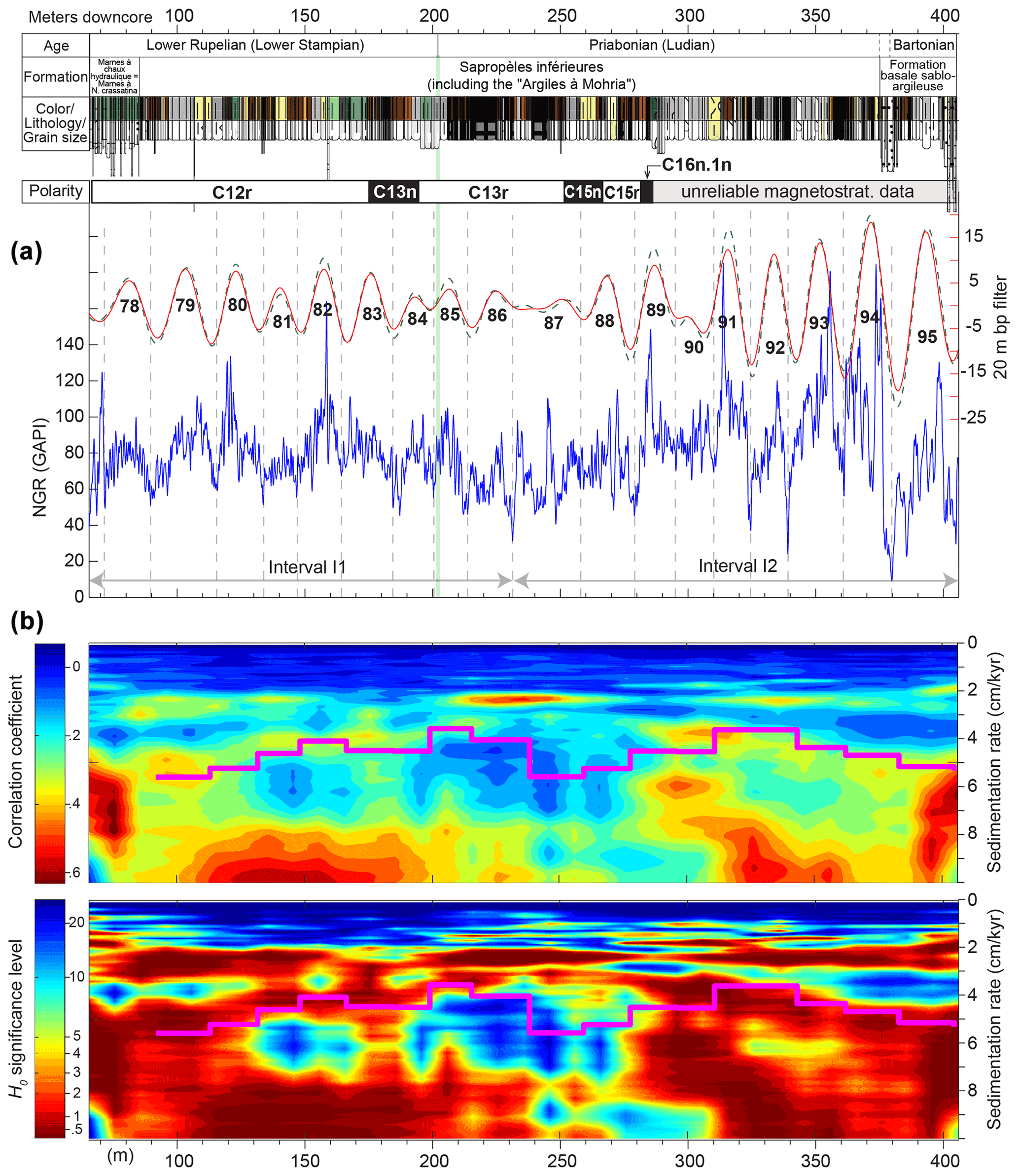
Figure 2(a) Integrated cyclo-magnetostratigraphy of the CDB1 drill core. Paleomagnetic data are provided in the Supplement. For sediment color, lithology and grain size, see Bauer et al. (2016). On the natural gamma radiation (NGR) data (10 cm resolution) a Gaussian band-pass filter (0.05 ± 0.015 cycles per meter in solid line, 0.05 ± 0.02 cycles per meter in dashed line) is applied to extract the prominent cyclicity of a ∼ 20 m wavelength, interpreted as reflecting the 405 kyr eccentricity periodicity. The numbering scheme for the 405 kyr eccentricity cycles follows the approach of Hinnov and Hilgen (2012), where eccentricity maxima are counted back in time. Intervals I1 and I2 correspond to those used for time-series analysis in the depth domain (Fig. 3). (b) Statistical evolutive COCO outputs (see Methods). Upper panel: correlation coefficient, lower panel: null hypothesis H0. Stair-like curve in pink is the sedimentation rate inferred from the 405 kyr tuning of the 20 m wavelength shown in (a). The eCOCO parameters are 0–10 cm kyr−1 with an increment of 0.1 cm kyr−1 for testing sedimentation rates, window = 80 m, step = 1 m, 1000 Monte Carlo simulations. Note that the manual sedimentation rate tracks the statistically inferred eCOCO sedimentation rate, except for the interval at roughly 240–280 m, where the significance is very low. This is likely due to the poorly preserved cyclicities at the transition between 405 kyr cycles 86 and 87 and cycle 88 (see Fig. 3). For the estimated optimal mean sedimentation rate over the whole studied interval, see Fig. 4.
2.2 Biostratigraphic framework of the CDB1 core
Biostratigraphic constraints are provided by nearly one hundred stratigraphic levels sampled and analyzed throughout the core (Table S1; Bauer et al., 2016). The biostratigraphy relies on various fossils and microfossils, including malacofaunal assemblage, benthic foraminifera, dinocyst and pollen grain assemblages (Table S2). Most of the studied intervals rely on pollen constraints that are refined by comparison with well-dated basins from western Europe, especially with the nearby Paris Basin (see Bauer et al., 2016, and references therein). Depending on recovered fossil assemblages and sampling resolution, uncertainties on estimated age or biozone boundaries vary, ranging from less than 1 m for the top SBZ21 biozone to ca. 110 m for the Bartonian–Priabonian boundary (Table S2). The Priabonian–Rupelian boundary (Eocene–Oligocene boundary) is relatively well constrained by a marked biozone boundary bracketed between 195.08 and 205.99 m depth (Table S2).
3.1 Magnetostratigraphy
Sampling of ca. 220 standard paleomagnetic oriented cylinders (2.5 cm diameter and 4–10 cm long) was performed using an electric drill at regular 1–3 m intervals throughout the whole preserved portion of the core from 66–411 m depth.
Remanent magnetization of samples was measured on a 2G Enterprises DC SQUID cryogenic magnetometer within an amagnetic chamber, at the Geosciences Rennes paleomagnetic laboratory, France. A first selection of pilot samples distributed around 10 m intervals throughout the core was stepwise demagnetized both thermally and using alternative field (AF). A high-resolution set of demagnetization steps were initially applied in order to (1) determine the characteristic demagnetization behavior, (2) establish the most efficient demagnetization temperature and AF steps, (3) determine which lithology provides the best signal, and (4) identify stratigraphic intervals with potential paleomagnetic reversals. These preliminary results guided further processing of selected remaining samples at higher stratigraphic resolution. To better identify magnetic mineralogies, isothermal remanent magnetization (IRM) acquisitions separated into three coercivity components (1150, 400 and 125 mT) followed by thermal demagnetization were undertaken on a set of 10 representative samples (Lowrie, 1990; Fig. S2).
Characteristic remanent magnetization (ChRM) directions were calculated using a minimum of four consecutive heating steps on thermal demagnetization paths displayed on vector-end point diagrams (Fig. S1). A careful selection of ChRM directions (especially of normal directions) was performed by grouping them by quality: Q1 for reliable directions, Q2 for reliable polarities and Q3 for unreliable (see Fig. S1 for details). Great-circle analysis was applied to a few samples, when a secondary normal polarity component overlapped a reversed polarity direction carried by only a few points (the mean of the Q1 reverse polarity directions was used as set point following McFadden and Reid., 1982).
3.2 Natural gamma radiation (NGR)
Natural gamma radiation (NGR) in sedimentary rocks is due to gamma rays emitted via natural radioactivity mainly from potassium (K40), thorium () and uranium (). These elements are mainly present in clay minerals, and the NGR therefore essentially expresses the clay–carbonate ratio. NGR has been used successfully as a climatic proxy to detect orbitally forced sedimentation patterns and has served as a powerful tool for cyclostratigraphy and orbital tuning (e.g., van Vugt et al., 1998).
The NGR probe used during the CDB1 well logging consists of a scintillation detector (sodium iodide crystal coupled to a photo-multiplication tube), which converts gamma rays into electric pulses. The measured values are expressed in API (American Petroleum Institute) units (Fig. 2). These units are calculated using a linear interpolation of raw data expressed in pulses per second (pps) according to a calibration set with a very stable source, the radioactivity of which is known in API units. Because disintegration is a random phenomenon, raw measurements taken every 2 cm are integrated over a 25 cm long window and restored at a 10 cm step, which is consistent both with the crystal size and the average dip of the strata (∼ 15∘). The NGR dataset is available as Supplement.
3.3 Cyclostratigraphic analysis
To quantify significant wavelengths in sedimentary proxies that could be related to specific orbital frequencies, we used the multitaper method (MTM, Thomson, 1982) associated with the robust red noise modeling (Mann and Lees, 1996). Because of the high variability in the NGR signal throughout the core, we subdivided it into two intervals, I1 and I2 (Fig. 2). Then, to better visualize both lower and higher portions of the spectra, analyses were conducted with three 2π data tapers, using a logarithmic scale for the power axis (e.g., Fig. 3). To study the evolution of cycles throughout the record, we used evolutive harmonic analysis (EHA) with a function computing a running periodogram of a uniformly sampled (dx= 10 cm) time series using FFTs of zero-padded segments, and normalized to the highest amplitudes (e.g., Kodama and Hinnov, 2014; Fig. S8). To study the evolution of sedimentation rates throughout the core we used the COCO method (the correlation coefficient method, Li et al., 2018) to statistically check the manual interpretation of Milankovitch cycle bands. The COCO technique is an automatic frequency ratio method inspired from the average spectral misfit (ASM) of Meyers and Sageman (2007). It estimates the correlation coefficient between the power spectra of an astronomical target signal and paleoclimate proxy series across a range of tested sedimentation rates. As with ASM, a null hypothesis of no astronomical forcing is evaluated using Monte Carlo simulation. To extract target cycles, we used conjointly band-pass Gaussian filtering (Paillard et al., 1996) and the smoothing technique based on the weighted average LOWESS method (e.g., Fig. 3). Finally, to convert the depth into the time domain, we used the 405 kyr stable eccentricity period because it is well expressed along the whole core (Figs. 2 and S8), and its phase is very stable (Laskar et al., 2004, 2011). First, we tuned the NGR record to a pure 405 kyr target sine curve. Next, we anchored the obtained floating timescale of the calibrated NGR record to previously proposed ages of EOB. Then, we established several potential correlations between the 405 kyr cycles from NGR and La2011 astronomical model, in order to seek for the best fit using the cross-MTM spectral analysis (e.g., Huybers and Denton, 2008). Based on the retained age of EOB that provides the reasonable phase between the NGR and the orbital eccentricity variations (Sect. 5.1), we finally adjusted the EOB anchored floating timescale to the orbital solution by tuning the 405 kyr cycle extremes in the NGR to their time equivalents in the astronomical signal. We have also tested the continuity of the CDB1 core by comparing the 405 kyr tuning with 21 kyr tuning (precession mean period, Fig. S7c).
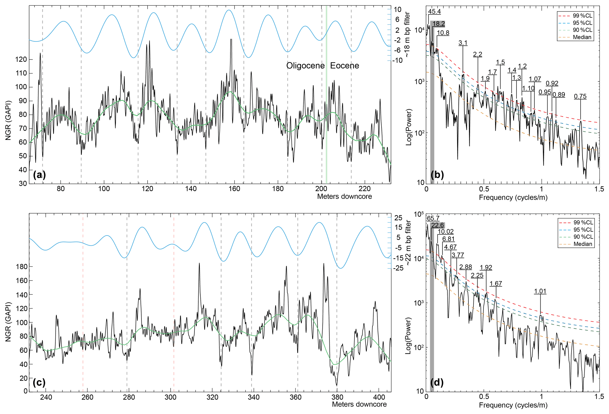
Figure 3Time-series analysis per interval I1 (65.5–232 m) and I2 (232–406 m (see Fig. 2)) of the untuned NGR variations. (a) Interval I1, along with 18.2 m band-pass filtered (as in Fig. 2) and smoothed with a 8 % weighted average of the series. (b) 2π-MTM power spectrum of interval I1. (c) Interval I2, along with 22.6 m band-pass filtered (as in Fig. 2) and smoothed with a 8 % weighted average of the series. (d) 2π-MTM power spectrum of interval I2. Grey-shaded vertical bars in (b) and (d) correspond to the filtered cyclicity in (a) and (c). All spectral periods in (b) and (d) are expressed in meters.
4.1 Rock magnetism analyses and magnetostratigraphy
Initial natural remanent magnetization (NRM) was typically low (Table S3), ranging between 10−3 to 10−6 A m−1 and thus requiring the use of a highly sensitive cryogenic magnetometer. Lower NRM values were generally recorded in the lower part of the core in particular below ca. 300 m depth where most samples yielded uninterpretable erratic demagnetization paths that can be attributed to their low NRM values, in the order of instrumental detection. Above ca. 300 m depth, however, most of the 114 samples analyzed yielded higher NRM values usually far above the detection level of the magnetometer (Table S3) with interpretable demagnetization paths. These thermal demagnetization diagrams (Fig. S1) generally display two main components: a low temperature component (LTC) from 0 to 150–180 ∘C and a higher temperature component (HTC) from 180–250 to 600 ∘C. However, above 300–350 ∘C, demagnetization paths often become erratic, showing unstable remanences with often increasing remanence intensities and increasing magnetic susceptibilities suggesting mineral transformation in most samples. AF demagnetization yielded less separation of LTC and HTC, with demagnetization becoming often erratic and noisy at high applied fields and some evidence for gyroremanence acquisition. As a result, thermal rather than AF demagnetization was applied to the remainder of the sample set with a carefully defined set of targeted small thermal demagnetization steps (Fig. S1). This procedure generally yielded demagnetization diagrams with clearly separated LTC and HTC although they sometimes overlapped along great circle paths on stereographic projections. LTC have exclusively normal polarity orientations suggesting a recent overprint while HTC display normal and reversed polarity orientations.
The nature of the magnetization components is further indicated by the IRM acquisition showing mostly low coercivities (<200 mT Fig. S2a). Its separation into three coercivities indicate most (70 %–90 %) of the IRM magnetization in the low coercivities (below 125 mT), 5 %–20 % in the intermediate (125–400 mT) and <10 % in the high coercivity (400–1150 mT). The thermal demagnetization of these IRM shows the following behaviors. (a) The low coercivity components are demagnetized monotonically down to 600 ∘C with some samples mostly demagnetized at 350–400 ∘C (Fig. S2b). (b) The intermediate coercivity has noisy demagnetization mostly achieved at 350–400 ∘C (Fig. S2c). (c) The high coercivity is more stable but also mostly demagnetized at 350–400 ∘C (Fig. S2d).
The observed behaviors lead us to interpret that the remanent magnetization is carried by a combination of iron oxides and iron sulfides. The presence of iron sulfides is strongly suggested by the organic-rich nature of the sediment and in particular, the observation of pyrite formation upon splitting of the cores and their surficial oxidation in the warehouse. Furthermore, the NRM thermal demagnetization increasing and becoming unstable in the 250–400 ∘C range are characteristic of iron sulfide oxidation thermally transforming into iron oxides upon thermal treatment (e.g. Dunlop and Özdemir, 1997). Gyroremanence acquisition during AF treatment of NRM potentially suggests greigite (Vasiliev et al., 2008; Sagnotti et al., 2010). However, the demagnetization of samples up to 600 ∘C indicates iron oxides also contribute to the remanence. This is further confirmed by IRM experiments. The low coercivity component carrying most of the signal is demagnetized up to 600 ∘C, suggesting magnetite. This low coercivity component may also partly include iron sulfides such as thermally stable single-domain greigite and pyrrhotite, which have coercivities below 200 mT indicative of either secondary or primary origin (Dekkers et al., 1988; Roberts et al., 1998). The intermediate and higher-coercivity components demagnetized below 400 ∘C may correspond to partial oxidation of pyrrhotite and greigite acquired during diagenetic weathering or more likely during the thermal demagnetization breaking down iron sulfides, which could explain the instability observed in this range (Roberts et al., 2011).
These considerations help us to interpret the observed LTC and HTC components. The LTC exclusively in a normal polarity direction can be simply explained by secondary iron sulfides formed during diagenetic processes (e.g. Roberts et al., 2011). The HTC is more complex as it likely relates to a combination of iron sulfides that may be primary or secondary and oxides that are likely primary. The magnetite present in the samples must contribute a large part of the NRM in the HTC range but it is blurred by iron sulfides that oxidize at these temperatures, becoming unstable and acquiring secondary magnetization that explains the difficulty of isolating the primary components in the HTC. Nevertheless, a stable HTC was often isolated after the LTC and before the directions became unstable at high temperatures (Fig. S1 in the supplement). This HTC is most likely carried by the magnetite present in the samples as indicated by stable thermal demagnetization up to 600 ∘C in a few samples with few iron sulfides. However, some of the HTC may be carried by iron sulfides making the demagnetization at times difficult to interpret such that careful inspection and defining quality criteria were applied to select HTC for further ChRM direction and polarity determinations (see Fig. S1 for the definition of the quality criteria).
The carefully selected ChRM directions obtained from the HTC yielded inclinations displaying two distinct clusters around +50 and −50∘ respectively as expected at this latitude and thus further suggest a primary record of normal and reversed polarities (Fig. S3). In order to remove widely outlying and transitional directions, the inclinations lying within −30 and +30∘ were rejected. The careful selection procedure finally resulted in a set of 70 ChRM directions providing reliable paleomagnetic polarity determination at regular intervals from ca. 66–290 m depths of the core. Polarity zones were then defined by at least two consecutive paleomagnetic sites bearing the same polarity such that isolated points were further discarded for the definition of polarity zones.
By considering the above magnetic analysis, six reliable polarity magnetozones including three normal (N1–N3) and three reversed (R0–R2) were identified in the section (Fig. S3). As a starting point for the correlation of our paleomagnetic results with the geomagnetic polarity timescale (GPTS, Vandenberghe et al., 2012; Ogg et al., 2016) we considered initial dating from fossil pollen biostratigraphy providing independent constraints. Intervals in the core were assigned depositional age ranges based on palynology; in particular the EOB is bracketed between 195.08 and 205.99 m depth (see Sect. 2.2, Table S2, Fig. 2). This interval is comprised near the top of the long reversed polarity zone R1. Above, the relatively short magnetozone N1 overlain by the long R0 provides the expected correlation to the distinctive Chron sequence C13r–C13n–C12r with the EOB near the top of C13r. The stratigraphic position of the Eocene–Oligocene boundary (EOB) is fixed by assuming that the EOB is situated 86 % up in Chron C13r (Luterbacher et al., 2004). According to the above correlation, the two short N2 and R2 magnetozones below would clearly correspond to Chrons C15n and C15r respectively. Below magnetozone R2, the short N3 may consequently correspond to Chron C16n.1n (Fig. 2). Below magnetozone N3, a weak paleomagnetic signal with unreliable demagnetization behavior prevented a clear magnetostratigraphic pattern from being established.
4.2 Natural gamma radiation (NGR) variations
NGR values in the studied 65.5–406 m interval vary from ca. 50 API to ca. 100 API, sometimes reaching greater values but always <200 API. NGR variations show strongly cyclic patterns with multiple wavelengths and variable amplitudes. In particular, a ∼ 20 m thick cyclicity is prominent throughout the core, on which are superimposed high-frequency cycles (Figs. S4, S5). Stronger amplitudes are encountered within the Priabonian Stage, especially in its lower part (Fig. S5). The Lower Rupelian sediments are also characterized by cyclic variations, readily identifiable (Fig. S4), but with lower amplitudes compared to the lower Priabonian interval.
The environmental significance of the NGR variations can be determined based on previous mineralogical and sedimentological results from the core (Tramoy et al., 2016; Ghirardi, 2016). XRD analyses were performed on the various facies along the core and on both bulk rock and the clay fraction (Tramoy et al., 2016). The clay minerals are largely dominated by kaolinite throughout the core but smectite suddenly appears at ∼ 199.5 m depth with large variations, sometimes in greater proportion than kaolinite (Tramoy et al., 2016). However, this abrupt change in clay mineral assemblage does not affect the NGR periodic signal. This is consistent with a fraction >90 % dominated by kaolinitic–smectitic that usually does not affect NGR (Hesselbo, 1996). Illite containing potassium is more commonly associated with NGR signal. However, no correlation could be found between illite and NGR variations, probably because, although present, illite varies little through the core (Tramoy et al., 2016).
In contrast, NGR is clearly anticorrelated to TOC values (Ghirardi, 2016). Although organic matter (OM) is well known for absorbing uranium from marine water in reducing oceanic settings, such anticorrelation (maximum TOC corresponding to minimum NGR) is not uncommon in lake settings and may attest for a diluting process of a U-rich clastic component in the sediment (e.g., Lüning and Kolonic, 2003). In any case, lower NGR intervals corresponding to higher TOC with enhanced organic matter productivity/preservation conditions are therefore interpreted to reflect protracted wetter periods and vice versa.
4.3 Time-series analysis
Power spectrum of the upper interval I1 (Fig. 3a, b) shows three significant (reaching the 99 % confidence level, CL) low-frequency peaks centered on 45.4, 18.2 and 10.8 m. At higher frequencies, we note a multitude of significant (above 95 % CL) peaks of wavelengths varying from 0.75–3.1 m. The power spectrum of the lower interval I2 (Fig. 3c, d) shows four significant (above 99 % CL) low-frequency peaks of 65.7, 22.6, 10.02 and 6.81 m. At higher frequencies, we note a distinct peak centered on 1.01 m, and several other significant (above 95 % CL) peaks of wavelengths ranging from 1.67–4.67 m.
Filtering, smoothing and visual inspection (Fig. 3a, c) point to a prominent, continuous cyclicity detected by the ∼ 20 m peak (the mean of 18.2 m in Fig. 3b and 22.6 m in Fig. 3d). Visual inspection of well-expressed ∼ 20 m cycles allows the identification of about 20 high-frequency ∼ 1 m cycles within almost each of the ∼ 20 m cycle (Figs. S4, S5). This is consistent with the ∼ 20 m cycles corresponding to 405 kyr eccentricity cycles, and the high-frequency ∼ 1 m cycles to precession cycles. This cyclostratigraphic interpretation is further substantiated when applying previous timescales (e.g., Vandenberghe et al., 2012) to the recognized polarity chrons in the CDB1 core (Sect. 4.1). Additionally, the statistical COCO tests (Figs. 2, 4) detect an optimal sedimentation rate of 5.2 cm kyr−1, which is very close to the visually inferred mean sedimentation rate (i.e., 20 m for the 405 kyr eccentricity cycle). Calibrating the ∼ 20 m cyclicity to a single 405 kyr periodicity results in temporal spectral peaks (Figs. 5, S7a, b) sharing some similarities with the astronomical periods (Fig. S7c). In the interval I1, the precession cycle band (Fig. S7a) is characterized by periods ranging from 14–22 kyr, the obliquity cycle band between 25 and 54 kyr, and the short eccentricity is possibly detected by the two peaks of 72 and 92 kyr. Within the interval I2, precession corresponds to 17.6–19.61 kyr, the obliquity to 31.15–58.6 kyr, and the short eccentricity possibly to the three peaks at 72, 81 and 134 kyr. We also note two strongly significant peaks in depth and time domains (Fig. S6): the ∼ 10 m peak tuned to ∼ 200 kyr, and the ∼ 55 m peak tuned to ∼ 1020 kyr. The former matches a minor eccentricity term (2g2–2g5). The latter may correspond to a g1–g5 eccentricity term (e.g., Laskar et al., 2004; Abels et al., 2010). We further discussed such cyclicity in Sect. 4.4.
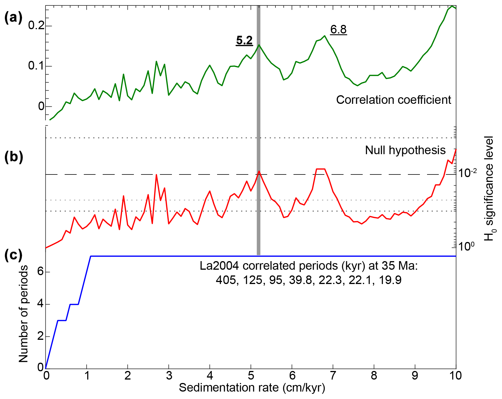
Figure 4Statistical testing for astronomical forcing hypothesis of NGR variations, and optimal sedimentation rate for orbitally forced NGR time series using the COCO technique (Li et al., 2018; see Methods). (a) Pearson correlation coefficient. (b) Null hypothesis H0. (c) Number of La2004 astronomical parameters used in the correlations (indicated). Note there are two optimal sedimentation rates at 5.2 and 6.8 cm kyr−1, which have significant H0 levels above 10−2. The optimal sedimentation rate at 5.2 cm kyr−1 (vertical grey bar) fits the visual mean sedimentation rate (see Fig. 2b).
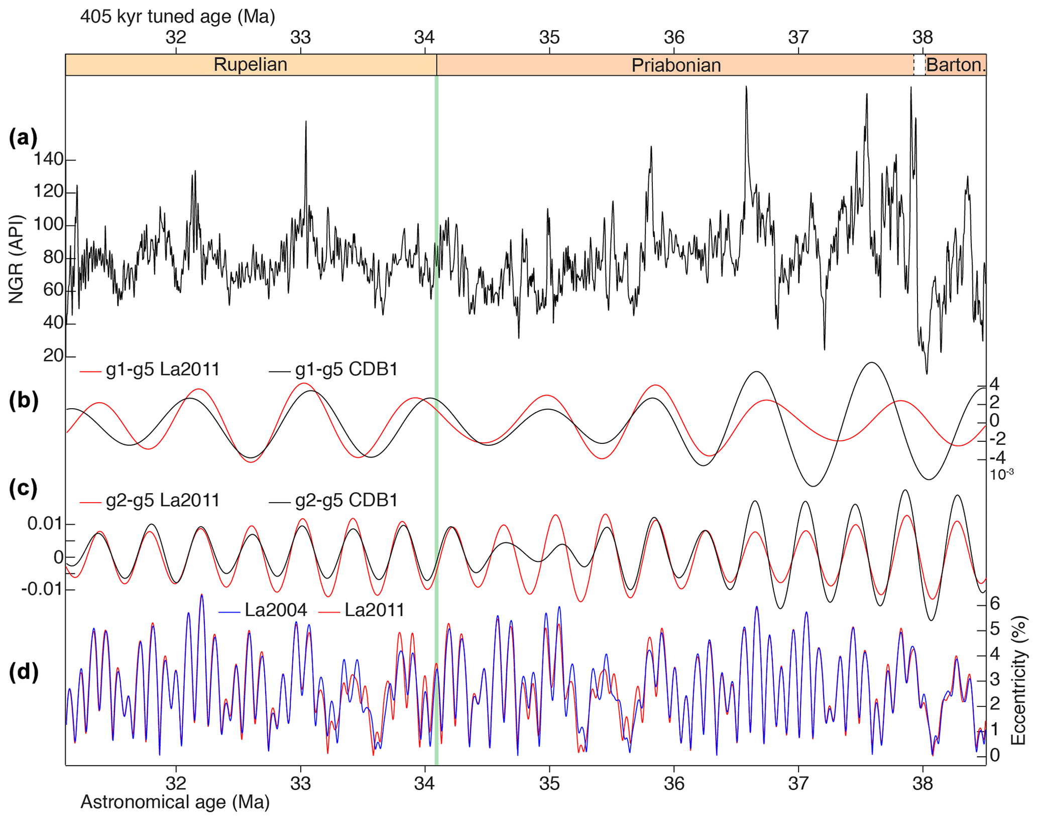
Figure 5Astronomical calibration of CDB1 core, along with filtering at 405 kyr (g2–g5) and ∼ 1 Myr (g1–g5) bands. (a) NGR data are tuned to a single 405 kyr sinusoid function and then anchored at the Eocene–Oligocene boundary at 34.10 Ma. The 34.10 Ma is the age showing the best phase relationship between the tuned NGR and La2004 orbital eccentricity curve (Laskar et al., 2004) at the 405 kyr cyclicity (Fig. S9; see Sect. 4.1 for detail). (b) Band-pass filtering at ∼ 1 Myr band. (c) Band-pass filtering at 400 kyr band. (d) Raw La2004 and La2011 orbital eccentricity data (Laskar et al., 2004, 2011).
In summary, spectral analysis of the 405 kyr tuned NGR time series shows consistent precession, obliquity and short eccentricity cycle bands despite potentially missing a few precession cycles by the intrinsic lake responses (e.g., Wang et al., 2020). Additionally, tuning to the 21 kyr mean precession period provides periods of 406 kyr and ∼ 1 Myr for g2–g5 and g1–g5 respectively (Sect. 4.4), thus pointing to the completeness of CDB1 record.
4.4 Astronomical calibration of the CDB1 core
The 405 kyr tuning of the NGR data provides a total duration of CDB1 core (interval from 65.5 to 406 m) of ∼ 7.6 Myr. Durations of the recognized Chrons C12n through C16n.1n, are comparable to estimates from previous studies (Sect. 4.5). Interestingly, we have noted within this time interval the same number of 405 kyr eccentricity cycles, as in deep-sea sequences (Pälike et al., 2006; Westerhold et al., 2014). To make the comparison easier we followed the same numbering scheme of the 405 kyr eccentricity (Fig. 2), where eccentricity maxima are counted back in time (Hinnov and Hilgen, 2012). In the CDB1 core, Chron C12r through Chron C15r span cycles 78–88, exactly the same result as that obtained from the eastern equatorial Pacific, Site 1218 (Pälike et al., 2006), and from the Pacific Equatorial Age Transect (PEAT, IODP Exp. 320/321, Westerhold et al., 2014). Therefore, most of the 405 kyr eccentricity cycles recorded in the CDB1 core seem to be complete (consisting of about 20 precession cycles; see Fig. S4). Because the precession frequency is not defined with precision for the studied time interval (Laskar et al., 2004), our strategy for the astronomical calibration of the core was mainly based on the 405 kyr (first-order) eccentricity cycles. Then, because of the strong expression of the precession signal, a 21 kyr tuning was performed to refine the 405 kyr calibration of polarity chrons (Sect. 4.5), but only on intervals overlapping parts of 405 kyr cycles. These intervals concern cycles 83, 84, 87, 88 and 89, which seem to be complete. Short eccentricity cycles are not as continuously expressed as the 405 kyr cycles, possibly because the obliquity played a role in obliterating precession modulation. Therefore, short eccentricity cycles were not used for orbital tuning.
The 405 kyr eccentricity tuning of the CDB1 core calibrates the longest cyclicity (∼ 50 m thick) to a period of ∼ 1 Myr (Figs. 5 and 6), supporting the expression of g1–g5 in continental environments. In particular, detailed cyclostratigraphic study of middle Miocene fluvial to lacustrine sedimentary sequences in northeastern part of the Madrid Basin (Spain) detected with high fidelity 405 kyr (g2–g5), 0.97 Myr (g1–g5) and 2.4 Myr (g4–g3) eccentricity cycles (Abels et al., 2010).
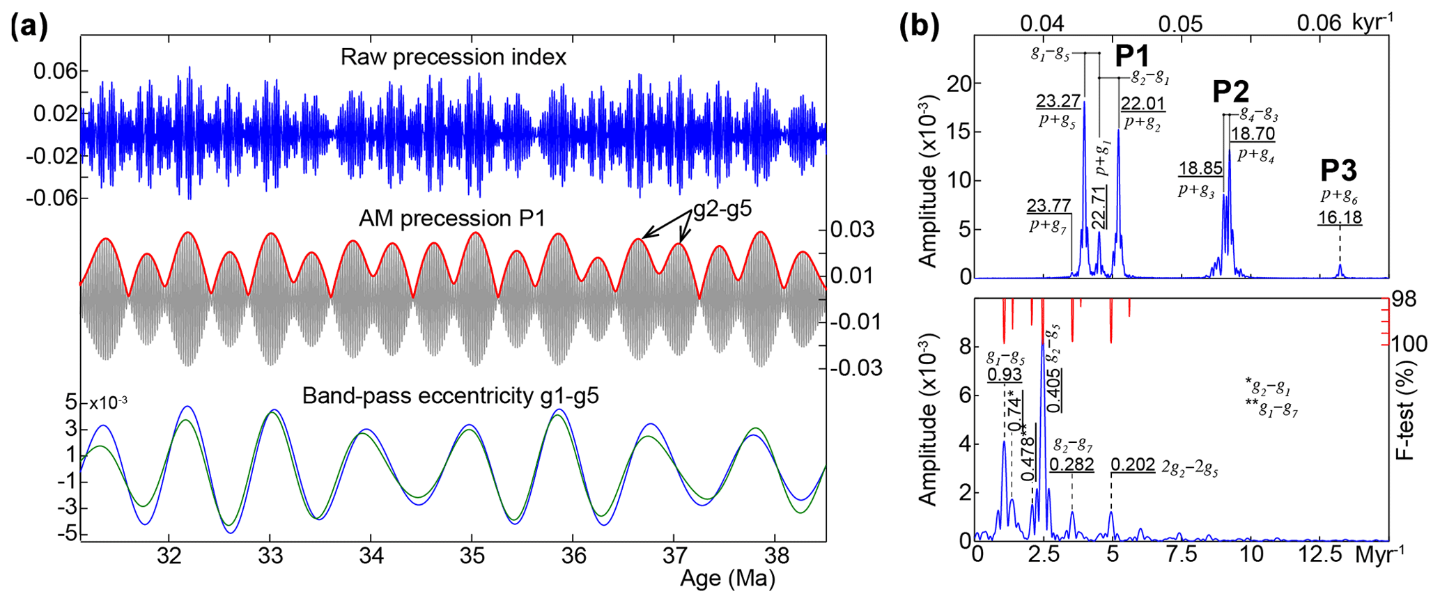
Figure 6Amplitude modulation (AM) of the precession index band P1. (a) La2004 precession index (Laskar et al., 2004), AM of precession P1 band (cut-off frequencies: 0.044 ± 0.002 cycles every thousand years), and band-pass filtering of the g1–g5 eccentricity component (cut-off frequencies: 0.00115 ± 0.0003 cycles every thousand years) from AM precession P1 (blue curve) and from the raw eccentricity (green curve). (b) 2π-MTM amplitude spectra of the raw precession index (upper panel) and AM precession P1 (lower panel).
It seems that the expression of certain eccentricity terms, especially g1–g5, arises from strong imprint of some specific precession components. In particular, longer precession components are likely to be better documented than the shorter ones, especially in the context of lower sedimentation rates (Boulila et al., 2008). The two strongest (largest) precession components are p+g5 (23.64 kyr) and p+g2 (22.31 kyr) and, together with a third long component p+g1 (23.07 kyr), would produce eccentricity modulation terms of three combinations of g2–g5 (405 kyr), g1–g5 (0.97 Myr) and g2–g1 (0.69 Myr) periods (Fig. 5). The CDB1 core documents g2–g5 and g1–g5 eccentricity terms with the greatest amplitudes (Fig. 7), pointing to the importance of these two periodic terms in continental lacustrine records. However, the CDB1 record does not document the 1.2 Myr obliquity nor the 2.4 Myr eccentricity cycles (Abels et al., 2010; Wang et al., 2020).

Figure 72π-MTM power spectra of the entire tuned raw NGR data. (a) Upper spectrum of the 21 kyr precession (Fig. S7c) tuned NGR, (lower) spectrum of the 405 kyr tuned NGR. (b) Upper and middle spectra are the same as in (a) but for the interval 0–0.015 cycles/kyr and in a linear-scale power axis, to highlight the low-frequency portion of the spectra. Lower spectrum of La2004 eccentricity over the equivalent time interval (31.110–38.501 Ma). Secular frequency for each eccentricity component is given, except for the short eccentricity (e), which has several components (e.g., Laskar et al., 2004).
In addition, we have noticed that sedimentary facies evolution (Bauer et al., 2016) sometimes matches the g2–g5 and sometimes the g1–g5 eccentricity terms, supporting the idea of sensitivity of lake level to longer cyclicities (Wang et al., 2020). Thus, we suggest that the paleolake level may have behaved as a low-pass filter for orbital forcing. Nevertheless, the expression of g1–g5 eccentricity in the lacustrine record remains to be investigated. Future cyclostratigraphic studies should focus on the expression of three specific eccentricity components, g2–g5, g1–g5 and g2–g1, in highly resolved continental records.
4.5 Durations of C12r through C16n.1n
Below we compare the CDB1 timescale with previous astronomical timescales in terms of calibrated durations of Chrons C12r through C16n.1n (Table 1). A recent study of Sahy et al. (2020) has shown difficulties in the quantification of ages of Chrons C12n through C16n.2n, even when integrating astronomical and radioisotopic dating. Accordingly, we have preferred to discuss durations of chrons rather than their ages (Table 1). The recent GTS2020 (Gradstein et al., 2020) uses the age model of Westerhold et al. (2014) for magnetic polarities C12r through C16n.1n. Thus, we below discuss durations of these chrons in the geological timescales prior to GTS2020 (Gradstein et al., 2020), together with the original cyclostratigraphic studies from which those estimates were inferred.
Table 1Durations of Chrons C12r through C16n.1n inferred from CDB1 core cyclostratigraphy and in comparison with previous timescales. Geomagnetic Polarity Time Scales: CK95 (Cande and Kent, 1995), GPTS2004 (Ogg and Smith, 2004) and GPTS2012 (Vandenberghe et al., 2012), Astronomical Time Scale (ATS): HP2006 from ODP Site 1218 (Pälike et al., 2006), TW2014 from ODP PEAT sites (Pacific Equatorial Age Transect, Exp. 320) (Westerhold et al., 2014). Magnetostratigraphic and radioisotopic dating: WRG and UMB are White River Group and Umbria–Marche Basin respectively (Sahy et al., 2020). Note that durations of all these chrons in GTS2020 (Gradstein et al., 2020) are from Westerhold et al. (2014) and subsequently used in Westerhold et al. (2020).
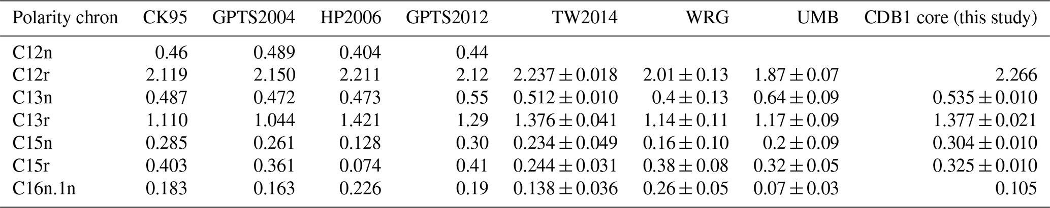
The duration of Chron C12r is very close to estimates derived from orbital tuning of ODP Site 1218 (Pälike et al., 2006) and PEAT sites (Westerhold et al., 2014), but longer than other estimates, e.g., 0.146 Myr longer than in CK95 (Cande and Kent, 1995) and GTS2012 (Vandenberghe et al., 2012). Both studies at Site 1218 and PEAT sites used well-expressed 405 kyr orbital eccentricity cycles in physical and chemical proxies to infer durations of 2.211 and 2.237 ± 0.018 Myr respectively, which are very close to the 2.256 Myr obtained here in the CDB1 core.
The duration of Chron C13n in the CDB1 core is estimated to be 0.535 Myr, which is consistent with recent estimates, 0.550 Myr (Vandenberghe et al., 2012) and 0.512 ± 0.010 Myr (Westerhold et al., 2014). These durations are, however, longer than those proposed by older studies, which yielded durations of 0.472, 0.473 and 0.487 Myr (Table 1). In fact, the duration of 0.473 Myr proposed by Pälike et al. (2006) using orbital tuning of Site 1218 was revised by Westerhold et al. (2014) using the PEAT data, and additional ODP sites including Site 1218. Therefore, Chron C13n would have a duration between ca. 0.50 and 0.55 Myr.
The duration of Chron C13r in the CDB1 core is assessed at 1.377 ± 0.021 Myr, which is similar to estimates from Site 1218 (Pälike et al., 2006) and PEAT sites (Westerhold et al., 2014), but much shorter than durations proposed in other timescales, e.g., CK95 and GTS2004 (Table 1).
The duration of Chron C15n assessed here at 0.304 ± 0.010 Myr is identical to GTS2012 (Vandenberghe et al., 2012), but longer than other duration estimates. Duration of Chron C15r in the CDB1 core is estimated at 0.325 ± 0.010 Myr, which is shorter than those inferred from previous GPTS, but longer than previous ATS estimates (Pälike et al., 2006; Westerhold et al., 2014). In contrast, the duration of Chron C16n.1n estimated in the CDB1 core at 0.105 Myr is much shorter than all previous timescales.
In summary, durations of Chrons C12r, C13n and C13r are going towards a stable orbitally tuned timescale, where estimates from the continental CDB1 record are very consistent with previous estimates inferred from orbital tuning of deep-sea sequences. However, durations of Chrons C15n, C15r and C16n.1n, as mentioned in a previous study (Westerhold et al., 2014), still suffer from uncertainty. The CDB1 core provides additional constraints on durations of C15n and C15r, but the duration of C16n.1n is too short (reduced) to be retained.
5.1 The age of the Eocene–Oligocene boundary
The late Eocene-early Oligocene timescale still lacks precision, and the age of the Eocene–Oligocene boundary (EOB) is not yet fixed; thus several estimates ranging from 33.714 to 34.1 Ma have been proposed (Table S4; see Hilgen and Kuiper, 2009 for a review). In particular, the late Eocene timescale has proven difficult to tune in several ocean drilling programs because of the shallow position of the calcite compensation depth (CCD) preventing deposition of carbonate-rich sequences suitable for application of integrated bio-cyclostratigraphy and stable isotopic stratigraphy (Pälike and Hilgen, 2008; Boulila et al., 2018). Although recent efforts have been made to tune this time interval from the Pacific Equatorial Age Transect (PEAT, IODP Exp. 320/321, Pälike et al., 2010), more precision is still needed to refine this key part of the Paleogene–Neogene (Westerhold et al., 2014).
Since astronomical calibration of the middle–late Eocene is not well-constrained in GTS2012, Vandenberghe et al. (2012) preferred to calculate ages for Chron boundaries using the synthetic marine magnetic anomalies profile of Cande and Kent (1995) and an interpolation between the nearest older and younger astronomically dated Chron boundary (i.e., C21n(o) at 47.8 Ma, and C13n(o) at 33.705 Ma). This combined Paleogene age model resulted in an age estimate of 33.9 Ma for the EOB. This age is retained in later geological timescales GTS2016 (Ogg et al., 2016) and GTS2020 (Gradstein et al., 2020). Orbital tuning of middle Eocene to early Oligocene using mainly data from the PEAT sites arrived at a close age of 33.89 Ma for the EOB (Westerhold et al., 2014). A younger 33.714 Ma age has been proposed by Jovane et al. (2006) on the basis of tuning the Rupelian GSSP of Massignano and is also close to one option of van Mourik et al. (2006) from the Massicore, drilled ∼ 100 m south of the Massignano section. In addition, van Mourik et al. (2006) provided another older age option of 34.1 Ma. A more recent study (Sahy et al., 2017) re-evaluated the late Eocene through Oligocene timescale using integrated radioisotopic and cyclostratigraphic data to reach an age of 34.09 ± 0.08 Ma for the EOB.
Our cross-correlations between the 405 kyr CDB1 timescale anchored at all these previously proposed EOB ages (Table S4) and the Earth's orbital eccentricity shed some light on these controversies. Results of cross-correlations between NGR and astronomical variations are summarized in Fig. S9. The 33.90 and 33.89 Ma ages (and to a lesser extent the 33.95 Ma) of the Eocene–Oligocene boundary (EOB) both show opposite phase relations between the NGR and eccentricity but the 33.714 Ma and 34.1 Ma EOB ages are approximately in phase. The other proposed ages imply NGR and eccentricity that are neither in phase nor in opposite phase. We deduce that the optimal EOB ages in terms of phase relationship between the NGR and astronomical signal are either 33.714 and 34.10 Ma that are in phase with eccentricity or 33.90 and 33.89 Ma that are in opposite phase (Fig. S9). We can further refine this selection by considering 405 kyr eccentricity cycle maxima as responsible for stronger amplitude precession and insolation cycles, and thus intensified seasonality with longer drier seasons. Based on a pollen assemblage proxy, the prevailing climatic conditions within the studied interval (or at least from 66.85–265.90 m) were dry (Bauer et al., 2016). Thus, increasing the range between dry- and wet-season precipitation over land and its effect on vegetation primary productivity is likely, leading in general to longer and more intense dry seasons (e.g., Murray-Tortarolo et al., 2016). Following the anticorrelation of NGR and TOC and the hypothesis of cyclically diluted NGR by the organic matter (Sect. 4.2), such an astroclimatic link would favor higher NGR but lower TOC values during insolation maxima, related to reduced organic matter productivity/preservation conditions during protracted drier seasons. Accordingly, increased values of NGR would reflect higher values in the orbital eccentricity; i.e., NGR and eccentricity would be in phase and thus favor the 33.714 and 34.1 Ma EOB ages.
5.2 Environmental changes across the Eocene–Oligocene transition
Based on our age control we can investigate the precise timing of previously observed environmental changes at the CDB1 core (Tramoy et al., 2016; Fig. 8) and correlate them to the well-established EOT evolution in the marine record and associated climate interpretations. In marine records, the Eocene–Oligocene climate transition (EOT) is described in two major steps (Coxall et al., 2005; Katz et al., 2008). The first (older) step (or EOT-1, Katz et al., 2008) occurs in the upper part of Chron C13r. The second (younger) climatic step (or Oi-1, Miller et al., 1991; Zachos et al., 1996), which represents the major shift in δ18O, is recorded around the base of Chron C13n. The first step is associated with atmospheric cooling ascribed to declining atmospheric CO2 and leading to the second step marking the onset of the major Antarctic glaciation (DeConto and Pollard, 2003; Pearson et al., 2009; Ladant et al., 2014). The Oi-1 glacial event could be divided into two sub-steps, Oi-1a and Oi-1b (Zachos et al., 1996; Coxall and Wilson, 2011). High-resolution δ18O data from the eastern equatorial Pacific (Coxall and Wilson, 2011) compared to other δ18O data mainly from the Southern Ocean (e.g., Zachos et al., 1996) further confirm the two-step structure of the EOT, but support in addition an EOT precursor ice growth event (Sect. 5.3) within Chron C13r (see Katz et al., 2008; Peters et al., 2010; Pusz et al., 2011).
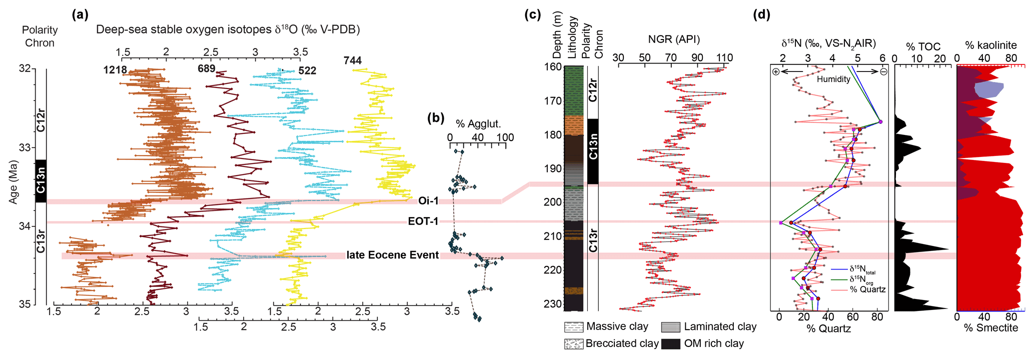
Figure 8Correlation of the main changes in the sedimentary facies in the CDB1 core around the EOT and the main climatic (cooling/glacial) events recognized in deep-sea records (DSDP Site 522, ODP Sites 689, 744 and 1258). (a) Deep-sea δ18O data from multiple sites (indicated, Site 1218: Coxall and Wilson, 2011; Site 689: Diester-Haas and Zahn, 1996; Sites 522 and 744: Zachos et al., 1996) document successive glacial events: “late Eocene Event”, EOT-1 and Oi-1 related to the Antarctic Ice Sheet (Coxall and Wilson, 2011). (b) Agglutinated benthic foraminifera data at ODP Site 647 (Kaminski and Ortiz, 2014) against the age model of Coxall et al. (2018). (c) Lithostratigraphy, magnetostratigraphy and NGR data around the Eocene–Oligocene boundary in the CDB1 core. (d) Terrestrial-derived organic nitrogen isotope record (δ15Norg), quartz content, total organic carbon (TOC) content, kaolinite and smectite contents from Tramoy et al. (2016).
The CDB1 core exhibits significant changes in the sedimentary facies around the EOT (Bauer et al., 2016). In particular, two prominent sedimentary facies changes occurring slightly below and above the EOB respectively. We estimate the duration of the interval between the two facies changes to 0.268 Myr. This interval comprises 13 well-expressed precession cycles, further supporting a duration of around 0.27 Myr. This compares nicely with marine records of steps EOT-1 and Oi-1 below and above the EOB, separated by about 0.25 Myr (Katz et al., 2008; Coxall and Wilson, 2011). Therefore, these two sedimentary changes in the CDB1 core most likely reflect the two major climatic steps EOT-1 and Oi-1. We note that Oi-1a, Oi-1b and the EOT precursor event do not appear to be expressed by lithological changes at CDB1.
The first step, below the EOB (205.5 m) (Fig. 8), is expressed as a gradual but rapid decrease in TOC (from black, organic-rich clays, to light-grey, whitish clays in a few decimeters). The second change above the EOB, which occurs at depth 195.26 m, is expressed by a sharp contact between massive, clotted greenish clay (palustrine facies) and overlying brownish, organic laminated clays (deep lacustrine facies). Previously acquired environmental proxies across the EOT at CDB1 show a TOC decrease, the appearance of smectite at the expense of kaolinite and a significant δ15N increase (Tramoy et al., 2016). The EOT is also marked by a strong development of conifers and the development of Ephedraceae and Umbelliferae (Bauer et al., 2016). Together these proxies have been interpreted as a rapid transition from humid and warm to drier and cooler climatic conditions with increased seasonality. In detail, the first step corresponds to the onset of the δ15N increase, a sharp TOC decrease and coeval increase in quartz contents from ∼ 13 %–∼ 49 % suggesting drying, dwindling vegetation cover and enhanced erosion in the catchment respectively. At the second step, δ15N continues to increase but a step cannot be deciphered due to insufficient sampling resolution (note different position of the second step in Tramoy et al., 2016). However, a step is clearly picked up by quartz content showing another major rapid increase from ∼ 20 %–∼ 70 %, suggesting, together with δ15N, further drying and catchment erosion while TOC remains low (∼ 0.5 %–∼3 %), and later recovery (∼ 12 %) (Fig. 8). Increased sediment input and drainage perturbation is also suggested by increased accumulation rates between the two steps before reaching steady deep lacustrine facies. This highlights the instability during this transition between climate states. Interestingly, the smectite signal seems delayed, appearing 6 m (147 kyr) above the first step and becoming dominant at the expense of kaolinite only 15 m (357 kyr) after the second step, which may reflect lag time in clay formation, transport and accumulation.
In summary, CDB1 records atmospheric cooling, drying and increased seasonality through the EOT as previously documented, with local variations, in continental records worldwide (Pound and Salzmann, 2017; Toumoulin et al., 2021, and references therein). At the CDB1, drying may simply relate to decreased intensity of the hydrological cycle due to global temperature and CO2 decrease as expected by climate models (e.g., Ladant et al., 2014). Alternatively, the North Atlantic coastal location of the CDB1 site opens the possibility that observed environmental changes relate to rerouting of oceanic currents leading to increased latitudinal gradients associated with the onset of the ACC and/or to the onset of a proto-Atlantic Meridional Oceanic Circulation (AMOC; see Sect. 5.3; Abelson and Erez, 2017; Elsworth et al., 2017; Coxall et al., 2018).
In any case, the two recognized environmental step changes concur with the global impact of the EOT-1 and Oi-1 events on terrestrial environments expressed via the hydrological cycle (e.g., Xiao et al., 2010; Page et al., 2019; Licht et al., 2020). Drying expressed by δ15N seems to occur through both steps but vegetation appears mostly affected by EOT-1. Further CDB1 proxy (in particular temperature) analyses at higher resolution will be required to assess changes at specific steps to infer their potential forcing mechanisms. However, the EOT cannot be simplified as a suite of discrete steps because it is clearly imprinted by orbitally paced variability (Zachos et al., 2001b; Coxall et al., 2005, 2011) that also provides insight into the forcing mechanism as developed below.

Figure 9Time-series analysis focused on the Eocene–Oligocene transition (EOT) showing the switch from obliquity to precession eccentricity. (a) Tuned NGR time series for the interval from 186 to 232 m, anchored at the EOB age of 34.10 Ma, with band-pass filtering at the 100 and 400 kyr eccentricity, 40 kyr obliquity and 20 kyr precession bands (solid curves for NGR cycles and dashed curves for La2004 astronomical cycles). Shaded area indicates strong obliquity cycles. (b) Power spectrum and amplitude spectrogram of the detrended (400 kyr cycles removed) tuned NGR, with the interpreted astronomical cycles for the 100 kyr eccentricity (e), obliquity and precession. Periods in the spectrum are in kiloyears. Note the striking switch from obliquity-dominant to precession eccentricity cycles at the Eocene–Oligocene transition event 1 (EOT-1). The interval from the late Eocene glacial event (LEGE) to the EOT-1 records very weak precession, especially at the dark pink-shaded area.
5.3 Obliquity forcing preconditioned the EOT
Visual inspection of the NGR variations points to prominent obliquity-scale cycles (with very weak or no precession cycles) occurring in the upper part of Chron C13r, within the 405 kyr cycle no. 85 (Fig. 9). The dominance of the obliquity starts at ca. 216.5 m and ends ca. 205.5 m. Evolutive harmonic analysis of the interval spanning the 405 kyr cycles 84, 85 and 86 (186–232 m interval) highlights a switch from obliquity-dominant to precession-eccentricity-dominant cycles at EOT-1. In detail, from depth 232 to ∼ 216.5 m, NGR variations record precession, eccentricity and strong obliquity. From 216.5–205.5 m the precession signal is weak, and the obliquity dominates (see also Fig. S10). From 205.5–186 m, the precession is well expressed, and the eccentricity is stronger than the obliquity. The time span between the onset (beginning) of obliquity-dominant cycles and the EOT-1 equivalent level (Sect. 5.2) is 0.280 Myr, which is of the same order than the 0.3 Myr proposed by Katz et al. (2008) between the EOT precursor glacial event (LEGE) and the EOT-1 (Figs. 8, 9). Accordingly, we suggest that the interval that documents the dominance of obliquity cycles corresponds to the LEGE–EOT-1 interval. This interval shows a gradual cooling confirmed by Peters et al. (2010), Pusz et al. (2011), and Coxall and Wilson (2011) on the basis of deep-sea data. In addition, several studies have recognized obliquity forcing in the latest Eocene terrestrial and marine records and argued it may relate to the presence of polar ice preconditioning the EOT (e.g., Abels et al., 2011; Jovane et al., 2006; Brown et al., 2009). Results from the CDB1 core lend support to the idea of obliquity forcing before EOT-1 but its cause and potential significance for the EOT remains to be determined amongst competitive mechanisms.
On the one hand, the global effect of large Antarctic ice-volume variations dominated by obliquity before its continental-scale coalescence may have modified the continental hydrological cycle and eustasy (e.g., deConto and Pollard, 2003; Ladant et al., 2014). After the ice-sheet formation at Oi-1, less important changes in ice volume would have ended obliquity dominance over precession-eccentricity forcing. This supposes that polar ice had formed earlier than EOT-1 in response to a more gradual CO2 decrease (e.g., Pound and Salzmann, 2017). In addition, these orbitally forced eustatic variations during early opening of the shallow Drake Passage may have also enabled incipient periodic ACC installation (Toumoulin et al., 2020).
On the other hand, the pre-EOT-1 obliquity interval may relate to the onset of North Atlantic Deep Water (NADW) production, driven either by the opening of the Drake Passage (Abelson and Erez, 2017; Elsworth et al., 2017) or tectonic adjustments allowing southward flow of cold and nutrient-laden Arctic water, fueling a proto-AMOC (Coxall et al., 2018). The latter hypothesis would have led to northward heat transport responsible for Antarctic cooling preconditioning the EOT. Multi-proxy study of North Atlantic sites suggests North Atlantic deep water formation starting at the LEGE and ending at EOT-1 (e.g., Kaminski and Ortiz, 2014; Coxall et al., 2018), precisely like the obliquity dominant interval at CDB1. Specifically, a remarkable decline in agglutinated benthic foraminifera in the southern Labrador Sea was ascribed to increased seawater cell convection in relation with the formation of deep waters (Fig. 8b, Kaminski and Ortiz, 2014; onset of regime 3 in Coxall et al., 2018). This abrupt biotic turnover shift is ∼ 630 kyr older than the EOB (Coxall et al., 2018 their Fig. 3f). In the continental CDB1 core, obliquity started to dominate ∼ 650 kyr before the EOB (Fig. 9). This remarkably coincident timing leads us to suggest the obliquity-dominated CDB1 interval supports the NADW formation hypothesis. This is substantiated by (1) the CDB1 location being directly affected by NADW, (2) the NADW sensitivity to obliquity and (3) the expected westerly moisture source of CDB1 being governed by the NADW (e.g., Abelson and Erez, 2017). Nevertheless, this hypothesis still needs further investigations from other terrestrial sites, deep-sea data records and climate modeling.
A ∼ 7.6 million-year-long lacustrine gamma radiation (NGR) record spanning the late Eocene (latest Bartonian to Priabonian) to the earliest Oligocene (early Rupelian) from a drill core (CDB1) in the Rennes Basin (northwestern France) documents with high fidelity the astronomical frequencies (precession, obliquity and eccentricity). The stable 405 kyr eccentricity is continuously expressed and thus used to astronomically calibrate this record.
The most prominent NGR cyclicity is calibrated to a period of ∼ 1 Myr matching a g1–g5 eccentricity term. Such cyclicity has been recorded in several continental records, pointing to its strong expression in continental depositional environments. The mechanisms transferring such cyclicity into the sedimentary lacustrine record remain elusive. Nevertheless, we suggest that the paleolake level may have exerted a low-pass filtering of the recorded astronomical variations since the low-frequency g1–g5 and sometimes the g2–g5 cyclicity are equally expressed in the sedimentary facies evolution.
Duration estimates of Chrons C12r through C16n.1n from the 405 kyr orbital tuning are consistent with previous estimates obtained from deep-sea sequences. This attests to the completeness of the CDB1 lacustrine record. Such an exceptional terrestrial record motivates us to suggest the CDB1 timescale as a continental reference in a future generation of Paleogene–Neogene timescales.
Assuming that maxima in NGR data reflect maxima in Earth's orbital eccentricity (maxima of insolation) and by anchoring the 405 kyr tuned NGR time series at different available ages of the Eocene–Oligocene boundary (EOB), we have noted that 33.714 and 34.10 Ma are the optimal ages providing the best phase fit between the NGR record and orbital eccentricity variations.
Improved calibrated age control enables us to identify that the EOT-1 and Oi-1 events are both marked by environmental changes (cooling, drying and enhanced seasonality) recorded in the CDB1 lithology and proxy records. This support previous claims that these events had a global impact on terrestrial environments via the hydrological cycle, though controlling mechanisms remain elusive. Detailed orbital study around the Eocene–Oligocene transition (EOT) highlights a pre-EOT interval dominated by obliquity over precession eccentricity, thus concurring with previous studies reporting similar patterns in terrestrial and oceanic environments, and their possible link with Antarctic glaciation preconditioning. At the end of this interval, the CDB1 core records for the first time a switch from obliquity to precession-eccentricity forcing at around the EOT-1 event. We thus potentially relate the obliquity-dominated interval to the instable phases of the incipient Antarctic Ice Sheet (AIS), whereas the onset of precession eccentricity dominance after EOT-1 would relate to a more stable, nearly coalesced AIS. These observations lead us to consider that obliquity variations preconditioned the EOT, either directly through AIS modulation or, preferably, via North Atlantic Deep Water formation.
The data set has been uploaded to a PANGAEA repository: https://issues.pangaea.de/browse/PDI-30098 (Boulila, 2021). Access is temporarily restricted but will be available at a later date.
The supplement related to this article is available online at: https://doi.org/10.5194/cp-17-2343-2021-supplement.
The paper was conceived and planned by SB and GDN, in collaboration with all authors. SB carried out the cyclostratigraphic analyses. GDN conducted the paleomagnetic study. SB, GDN, BG, HB and JJC contributed to the interpretations of data and finalization of the paper.
The contact author has declared that neither they nor their co-authors have any competing interests.
Publisher’s note: Copernicus Publications remains neutral with regard to jurisdictional claims in published maps and institutional affiliations.
This work originated from a project (CYNERGY Project) funded by the BRGM, the AELB and the ADEME. All the scientific crew is thanked for fruitful discussion. We thank the two reviewers and the editor Alberto Reyes for their constructive revisions.
Slah Boulila and Bruno Galbrun have been supported by ANR AstroMeso and ERC AstroGeo projects. Guillaume Dupont-Nivet has been supported by the Marie-Curie (CIG HIRESDAT and ERC MAGIC grants; grant no. 649081).
This paper was edited by Alberto Reyes and reviewed by two anonymous referees.
Abels, H. A., Abdul Aziz, H., Krijgsman, W., Smeets, S. J. B., and Hilgen, F. J.: Long-period eccentricity control on sedimentary sequences in the continental Madrid Basin (middle Miocene, Spain), Earth Planet. Sci. Lett., 289, 220–231, 2010.
Abels, H. A., Dupont-Nivet, G., Xiao, G., Bosboom, R., and Krijgsman, W.: Step-wise change of Asian interior climate preceding the Eocene–OligoceneTransition (EOT), Paleogeogr. Paleoclim. Paleoecol., 299, 399–412, 2011.
Abelson, M. and Erez, J.: The onset of modern-like Atlantic meridional overturning circulation at the Eocene–Oligocene transition: Evidence, causes, and possible implications for global cooling, Geochem. Geophys. Geosys., 18, 2177–2199, 2017.
Bauer, H., Bessin, P., Saint-Marc, P., Châteauneuf, J. J., Bourdillon, C., Wyns, R., and Guillocheau, F.: The Cenozoic history of the Armorican Massif: New insights from the deep CDB1 borehole (Rennes Basin, France), C. R. Geosciences, 348, 387–397, 2016.
Berggren, W. A., Wade, B. S., and Pearson, P. N.: Oligocene chronostratigraphy and planktonic foraminiferal biostratigraphy: historical review and current state-of-the-art, Cushman Foundation Special Publication, 46, 29–54, 2018.
Boulila, S.: Eocene-Oligocene continental sediment natural gamma radiation data of the CDB1 drill-core (Rennes Basin, France), PANGAEA [data set], available at: https://issues.pangaea.de/browse/PDI-30098, last access : 8 November 2021.
Boulila, S., Galbrun, B., Hinnov, L. A., and Collin, P.-Y.: Orbital calibration of the Early Kimmeridgian (southeastern France): implications for geochronology and sequence stratigraphy, Terra Nova, 20, 455–462, 2008.
Boulila, S., Vahlenkamp, M., De Vleeschouwer, D., Laskar, J., Yamamoto, Y., Pälike, H., Kirtland Turner, S., Sexton, P. F., and Cameron, A.: Towards a robust and consistent middle Eocene astronomical timescale, Earth Planet. Sci. Lett., 486, 94–107, 2018.
Brown, R. E., Koeberl, C., Montanari, A., and Bice, D. M.: Evidence for a change in Milankovitch forcing caused by extraterrestrial events at Massignano, Italy, Eocene–Oligocene boundary GSSP, in: The Late Eocene Earth–Hothouse, Icehouse, and Impacts, edited by: Koeberl, C. and Montanari, A., Geol. Soc. Am. Spec. Paper, 452, 1–19, 2009.
Cande, S. C. and Kent, D. V.: Revised calibration of the geomagnetic polar-ity timescale for the Late Cretaceous and Cenozoic, J. Geophys. Res., 100, 6093–6095, 1995.
Coxall, H. K. and Wilson, P. A.: Early Oligocene glaciation and productivity in the eastern equatorial Pacific: Insights into global carbon cycling, Paleoceanography, 26, PA2221, https://doi.org/10.1029/2010PA002021, 2011.
Coxall, H. K., Wilson, P. A., Pälike, H., Lear, C. H., and Backman, J.: Rapid stepwise onset of Antarctic glaciation and deeper calcite compensation in the Pacific Ocean, Nature, 433, 53–57, 2005.
Coxall, H. K., Huck, C., Huber, M., Lear, C., Legarda-Lisarri, A., O'Regan, M., Śliwińska, K., Flierdt, T., De Boer, A. M., Zachos, J. C., and Backman, J.: Export of nutrient rich Northern Component Water preceded early Oligocene Antarctic glaciation, Nat. Geosci., 11, 190–196, https://doi.org/10.1038/s41561-018-0069-9, 2018.
DeConto, R. M. and Pollard, D.: Rapid Cenozoic glaciation of Antarctica induced by declining atmospheric CO2, Nature, 421, 245–249, 2003.
Dunlop, D. J. and Özdemir, Ö.: Rock Magnetism: Fundamentals and Frontiers, Cambridge Univ. Press, New York, 573 pp., ISBN 9780521000987, 1997.
Dupont-Nivet, G., Krijgsman, W., Langereis, C. G., Abels H. A., and Fang, X.: Tibetan plateau aridification linked to global cooling at the Eocene–Oligocene transition, Nature, 445, 635–638, 2007.
Elsworth, G., Galbraith, E., Halverson, G., and Yang, S.: Enhanced weathering and CO2 drawdown caused by latest Eocene strengthening of the Atlantic meridional overturning circulation, Nat. Geosci., 10, 213–216, 2017.
Ghirardi, J.: Impact de la transition climatique Eocène-Oligocène sur les écosystèmes continentaux, Etude du Bassin de Rennes, PhD thesis, Université d'Orléans, Orléans, France, 332 pp., 2016.
Goldner, A, Herold, N., and Huber, M.: Antarctic glaciation caused ocean circulation changes at the Eocene–Oligocene transition, Nature, 511, 574–577, 2014.
Gradstein, F. M., Ogg, J. G., Schmitz, M. D., and Ogg, G. (Eds.): Geological Time Scale 2020, Elsevier, Amsterdam, the Netherlands, 2020.
Hesselbo, S. P.: Spectral gamma-ray logs in relation to clay mineralogy and sequence stratigraphy, Cenozoic of the Atlantic margin, offshore new jersey, in: Proc. ODP Sci. Results 150, edited by: Mountain, G. S., Miller, K. G., Blum, P., Poag, C. W., and Twichell, D. C., College Station, TX, (Ocean Drilling Program), USA, 411–422, https://doi.org/10.2973/odp.proc.sr.150.1996, ISSN 1096-7451, 1996. The ISSN is : 1096-7451
Hilgen, F. J. and Kuiper, K. F.: A critical evaluation of the numerical age of the Eocene–Oligocene boundary, in: The Late Eocene Earth–Hothouse, Icehouse, and Impacts, edited by: Koeberl, C. and Montanari, A., Geol. Soc. Am. Spec. Paper, 452, 1–10, 2009.
Hinnov, L. A. and Hilgen, F. J.: Cyclostratigraphy and astrochronology, in: The Geologic Time Scale 2012, edited by: Gradstein, F. M., Ogg, J. G., Schmitz, M., and Ogg, G., Elsevier, Amsterdam, the Netherlands, 63–83, 2012.
Hren, M. T., Sheldon, N. D., Grimes, S. T., Collinson, M. E., Hooker, J. J., Bugler, M., and Lohmann, K. C.: Terrestrial cooling in Northern Europe during the Eocene–Oligocene transition, P. Natl. Acad. Sci. USA, 110, 7562–7567, 2013.
Hutchinson, D. K., Coxall, H. K., Lunt, D. J., Steinthorsdottir, M., de Boer, A. M., Baatsen, M., von der Heydt, A., Huber, M., Kennedy-Asser, A. T., Kunzmann, L., Ladant, J.-B., Lear, C. H., Moraweck, K., Pearson, P. N., Piga, E., Pound, M. J., Salzmann, U., Scher, H. D., Sijp, W. P., Śliwińska, K. K., Wilson, P. A., and Zhang, Z.: The Eocene–Oligocene transition: a review of marine and terrestrial proxy data, models and model–data comparisons, Clim. Past, 17, 269–315, https://doi.org/10.5194/cp-17-269-2021, 2021.
Huybers, P. and Denton, G.: Antarctic temperature at orbital time scales controlled by local summer duration, Nat. Geosci., 1, 787–792, 2008.
Jovane, L., Florindo, F., Sprovieri, M., and Pälike, H.: Astronomic calibration of the late Eocene/early Oligocene Massignano section (central Italy), Geochem. Geophys. Geosys., 7, Q07012, https://doi.org/10.1029/2005GC001195, 2006.
Kaminski, M. and Ortiz, S.: The Eocene–Oligocene turnover of deep-water agglutinated foraminifera at ODP Site 647, Southern Labrador Sea (North Atlantic), Micropaleontology, 60, 53–66, 2014.
Katz, M. E., Miller, K. G., Wright, J. D., Wade, B. S., Browning, J. V., Cramer, B. S., and Rosenthal, Y.: Stepwise transition from the Eocene greenhouse to the Oligocene icehouse, Nat. Geosci., 1, 329–334, 2008.
Kodama, K. P. and Hinnov, L. A.: Rock Magnetic Cyclostratigraphy, New Analytical Methods in Earth and Environmental Science Series, John Wiley & Sons, Ltd., Hoboken, New Jersey, USA, ISBN 978-1-1185-6129-4, https://doi.org/10.1002/9781118561294, 2014.
Ladant, J. B., Donnadieu, Y., Lefebvre, V., and Dumas, C.: The respective role of atmospheric carbon dioxide and orbital parameters on ice sheet evolution at the Eocene–Oligocene transition, Paleoceanography, 29, 810–823, 2014.
Laskar, J., Robutel, P., Joutel, F., Gastineau, M., Correia, A. C. M., and Levrard, B.: A long-term numerical solution for the insolation quantities of the Earth, Astron. Astrophys., 428, 261–285, 2004.
Laskar, J., Gastineau, M., Delisle, J-B., Farrés, A., and Fienga, A.: Strong chaos induced by close encounters with Ceres and Vesta, Astron. Astrophys., 532, L4, https://doi.org/10.1051/0004-6361/201117504, 2011.
Lear, C. H., Bailey, T. R., Pearson, P. N. P., Coxall, H. K., and Rosenthal, Y.: Cooling and ice growth across the Eocene–Oligocene transition, Geology, 36, 251–254, 2008.
Li, M., Kump, L. R., Hinnov, L. A., and Mann, M. E.: Tracking variable sedimentation rates and astronomical forcing in Phanerozoic paleoclimate proxy series with evolutionary correlation coefficients and hypothesis testing, Earth Planetary Science Letters, 501, 165–179, 2018.
Licht, A., Dupont-Nivet, G., Meijer, N., Caves Rugenstein, J., Schauer, A., Fiebig, J., Mulch, A., Hoorn, C., Barbolini, N., and Guo, Z.: Decline of soil respiration in northeastern Tibet through the transition into the Oligocene icehouse, Palaeogeo. Palaeoclim. Palaeoecol., 560, 110016 https://doi.org/10.1016/j.palaeo.2020.110016, 2020.
Lowrie, W.: Identification of ferromagnetic minerals in a rock by coercivity and unblocking temperature properties, Geophys. Res. Lett., 17, 159–162, 1990.
Lüning, S. and Kolonic, S.: Uranium spectral gamma-ray response as a proxy for organic richness in black shales: applicability and limitations, J. Pet. Geol., 26, 153–174, 2003.
Luterbacher, H. P., Ali, J. R., Brinkhuis, H., Gradstein, F. M., Hooker, J., Monechi, S., Ogg, J. G., Powell, J., Röhl, U., Sanfilippo, A., and Schmitz, B.: The Paleogene Period, in: A Geologic Time Scale 2004, edited by: Gradstein, F., Ogg, J., and Smith, A., Cambridge University Press, Cambridge, UK, 384–408, 2004.
Mann, M. E. and Lees, J. M.: Robust estimation of background noise and signal detection in climatic time series, Climatic Change, 33, 409–445, 1996.
McFadden, P. L. and Reid, A. B.: Analysis of paleomagnetic inclination data, Geophys. J. R. Astron. Soc., 69, 307–319, 1982.
Meyers, S. R. and Sageman, B. B.: Quantification of deep-time orbital forcing by average spectral misfit, Am. J. Sci., 307, 773–792, https://doi.org/10.2475/05.2007.01, 2007.
Miller, K. G., Wright, J. D., and Fairbanks, R. G.: Unlocking the Ice House: Oligocene–Miocene oxygen isotopes, eustasy, and margin erosion, J. Geophys. Res., 96, 6829–6848, 1991.
Miller, K. G., Browning, J. V., Aubry, M.-P., Wade, B. S., Katz, M. E., Kulpecz, A. A., and Wright, J. D.: Eocene–Oligocene global climate and sea-level changes: St. Stephens Quarry, Alabama, Geol. Soc. Am. Bull., 120, 34–53, 2008.
Murray-Tortarolo, G., Friedlingstein, P., Sitch, S., Seneviratne, S. I., Fletcher I., Mueller, B., Greve, P., Anav, A., Liu, Y., Ahlström, A., Huntingford, C., Levis, S., Levy, P., Lomas, M., Poulter, B., Viovy, N., Zaehle, S., and Zeng, N.: The dry season intensity as a key driver of NPP trends, Geophys. Res. Lett., 43, 2632–2639, 2016.
Ogg, J. G. and Smith, A. G.: The geomagnetic polarity time scale, in: A Geological Timescale 2004, edited by: Gradstein, F. M., Ogg, J. G., and Smith, A. G., Cambridge University Press, Cambridge, UK, 63–86, 2004.
Ogg, J. G., Ogg, G., and Gradstein, F. M. (Eds.): A Concise Geologic Time Scale 2016, Elsevier, Amsterdam, the Netherlands, 2016.
Page, M., Licht, A., Dupont-Nivet, G., Meijer, N., Barbolini, N., Hoorn, C., Schauer, A., Huntington, K., Bajnai, D., Fiebig, J., Mulch, and Guo, Z.: Synchronous cooling and decline in monsoonal rainfall in northeastern Tibet during the fall into the Oligocene icehouse, Geology, 47, 203–206, 2019.
Paillard, D., Labeyrie, L., and Yiou, P.: Macintosch program performs timeseries analysis, Eos, 77, 379, https://doi.org/10.1029/96EO00259, 1996.
Pälike, H. and Hilgen, F. J.: Rock clock synchronization, Nat. Geosci., 1, 282, https://doi.org/10.1038/ngeo197, 2008.
Pälike, H., Norris, R. D., Herrle, J. O., Wilson, P. A., Coxall, H. K., Lear, C. H., Shackleton, N. J., Tripati, A. K., and Wade, B. S.: The Heartbeat of the Oligocene Climate System, Science, 314, 1894–1898, 2006.
Pälike, H., Nishi, H., Lyle, M., Raffi, I., Gamage, K., Klaus, A., and the Expedition 320/321 Scientists: Proc. IODP, 320/321: Tokyo, Integrated Ocean Drilling Program Management International, Inc., https://doi.org/10.2204/iodp.proc.320321.101.2010, 2010.
Pearson, P. N., Foster, G. L., and Wade, B. S.: Atmospheric carbon dioxide through the Eocene–Oligocene climate transition, Nature, 461, 1110–1113, 2009.
Peters, S. E., Carlson, A. E., Kelly, D. C., and Gingerich, P. D.: Large-scale glaciation and deglaciation of Antarctica during the Late Eocene, Geology, 38, 723–726, 2010.
Pound, M. J. and Salzmann, U.: Heterogeneity in global vegetation and terrestrial climate change during the late Eocene to early Oligocene transition, Scientific Reports, 7, 43386, https://doi.org/10.1038/srep43386, 2017.
Pusz, A. E., Thunell, R. C., and Miller, K. G.: Deep water temperature, carbonate ion, and ice volume changes across the Eocene–Oligocene climate transition, Paleoceanography, 26, PA2205, https://doi.org/10.1029/2010PA001950, 2011.
Roberts, A. P., Chang, L., Rowan, C. J., Horng, C.-S., and Florindo, F.: Magnetic properties of sedimentary greigite (Fe3S4): an update, Rev. Geophys., 49, RG1002, https://doi.org/10.1029/2010RG000336, 2011.
Sahy, D., Condon, D. J., Hilgen, F. J., and Kuiper, K. F.: Reducing Disparity in Radio-Isotopic and Astrochronology-Based Time Scales of the Late Eocene and Oligocene, Paleoceanography, 32, 1018–1035, 2017.
Sahy, D., Hiess, J., Fischer, A. U., Condon, D. J., Terry, D. O., Abels, H. A., Hüsing, S. K., and Kuiper, K. F.: Accuracy and precision of the late Eocene–early Oligocene geomagnetic polarity time scale, Geol. Soc. Am. Bull., 132, 373–388, 2020.
Sagnotti, L., Cascella, A., Ciaranfi, N., Macri, P., Maiorano, P., Marino, M., and Taddeucci, J.: Rock magnetism and palaeomagnetism of the Montalbano Jonico section (Italy): evidence for late diagenetic growth of greigite and implications for magnetostratigraphy, Geophys. J. Int. 180, 1049–1066, https://doi.org/10.1111/j.1365-246X.2009.04480.x, 2010.
Speijer, R. P., Pälike, H., Hollis, C. J., Hooker, J. J., and Ogg, J. G.: The Neogene Period, in: Geological Time Scale 2020, edited by: Gradstein, F. M., Ogg, J. G., Schmitz, M. D., and Ogg, G., Elsevier, Amsterdam, the Netherlands, 1087–1140, 2020.
Sun, J. M., Ni, X. J., Bi, S. D., Wu, W. Y., Ye, J., Meng, J., and Windley, B. F.: Synchronous turnover of flora, fauna, and climate at the Eocene–Oligocene boundary in Asia, Sci. Rep.-UK, 4, 7463, https://doi.org/10.1038/srep07463, 2014.
Thomson, D. J.: Spectrum estimation and harmonic analysis, IEEE Proc., 70, 1055–1096, 1982.
Toumoulin, A., Donnadieu, Y., Ladant, J. B., Batenburg, S. J., Poblete, F., and Dupont-Nivet, G., Quantifying the effect of the Drake Passage opening on the Eocene Ocean, Paleoceanography and Paleoclimatology, 35, e2020PA003889, https://doi.org/10.1029/2020PA003889 2020.
Toumoulin, A., Tardif, D., Donnadieu, Y., Licht, A., Ladant, J.-B., Kunzmann, L., and Dupont-Nivet, G.: Evolution of continental temperature seasonality from the Eocene greenhouse to the Oligocene icehouse – A model-data comparison, Clim. Past Discuss. [preprint], https://doi.org/10.5194/cp-2021-27, in review, 2021.
Tramoy R., Salpin, M., Schnyder, J., Person, A., Sebilo, M., Yans, J., Vaury, V., Fozzani, J., and Bauer, H.: Stepwise paleoclimate change across the Eocene–Oligocene Transition recorded in continental NW Europe by mineralogical assemblages and δ15Norg (Rennes Basin, France), Terra Nova, 28, 212–220, 2016.
Vandenberghe, N., Speijer, R. P., and Hilgen, F. J.: The Paleogene time scale, in: The Geologic Time Scale 2012, edited by: Gradstein, F. M., Ogg, J. G., Schmitz, M., and Ogg, G., Elsevier, Amsterdam, the Netherlands, 855–922, 2012.
van Mourik, C. A., Lourens, L. J., Brinkhuis, H., Pälike, H., Hilgen, F. J., Montanari, A., and Coccioni, R.: From greenhouse to icehouse at the Massignano Eocene–Oligocene GSSP: Implications for the cause, timing and effect of the Oi-1 glaciation, in: The Greenhouse-Icehouse Transition, A Dinoflagellate Perspective, edited by: van Mourik, C. A., PhD thesis, Stockholm University, Stockholm, no. 327, 32 pp., 2006.
van Vugt, N., Steebrink, J., Langereis, C. G., Hilgen, F. J., and Meulenkamp, J. E.: Magnetostratigraphy-based astronomical tuning of the early Pliocene lacustrine sediments of Ptolemais (NW Greece) and bed-to-bed correlation with the marine record, Earth Planet. Sci. Lett., 164, 535–551, 1998.
Vasiliev, I., Franke, C., Meeldijk, J. D., Dekkers, M. J., Langereis, C. G., and Krijgsman, W.: Putative greigite magnetofossils from the Pliocene epoch, Nat. Geosci., 1, 782–786, 2008.
Wang, M., Chen, H., Huang, C., Kemp, D. B., Xu, T., Zhang, H., and Li, M.: Astronomical forcing and sedimentary noise modeling of lake-level changes in the Paleogene Dongpu Depression of North China, Earth Planet. Sci. Lett., 535, 116116, https://doi.org/10.1016/j.epsl.2020.116116, 2020.
Westerhold, T., Röhl, U., Pälike, H., Wilkens, R., Wilson, P. A., and Acton, G.: Orbitally tuned timescale and astronomical forcing in the middle Eocene to early Oligocene, Clim. Past, 10, 955–973, https://doi.org/10.5194/cp-10-955-2014, 2014.
Xiao, G. Q., Abels, H. A., Yao, Z. Q., Dupont-Nivet, G., and Hilgen, F. J.: Asian aridification linked to the first step of the Eocene–Oligocene climate Transition (EOT) in obliquity-dominated terrestrial records (Xining Basin, China), Clim. Past, 6, 501–513, https://doi.org/10.5194/cp-6-501-2010, 2010.
Zachos, J. C., Quinn, T. M., and Salamy, S.: High-resolution (104 years) deep-sea foraminiferal stable isotope records of the Eocene-Oligocene climate transition, Paleoceanography, 9, 353–387, 1996.
Zachos, J. C., Pagani, M., Sloan, L., Thomas, E., and Billups, K.: Trends, Rhythms, Aberrations in Global Climate 65 Ma to Present, Science, 292, 686–693, 2001a.
Zachos, J. C., Shackleton, N. J., Revenaugh, J. S., Pälike, H., and Flower, B. P.: Climate response to orbital forcing across the Oligocene–Miocene boundary, Science, 292, 274–278, 2001b.