Simulation of the mid-Pliocene Warm Period using HadGEM3: experimental design and results from model–model and model–data comparison

Here we present the experimental design and results from a new mid-Pliocene simulation using the latest version of the UK's physical climate model, HadGEM3-GC31-LL, conducted under the auspices of CMIP6/PMIP4/PlioMIP2. Although two other palaeoclimate simulations have been recently run using this model, they both focused on more recent periods within the Quaternary, and therefore this is the first time this version of the UK model has been run this far back in time. The mid-Pliocene Warm Period, ∼3 Ma, is of particular interest because it represents a time period when the Earth was in equilibrium with CO₂ concentrations roughly equivalent to those of today, providing a possible analogue for current and future climate change.

The implementation of the Pliocene boundary conditions is firstly described in detail, based on the PRISM4 dataset, including CO₂, ozone, orography, ice mask, lakes, vegetation fractions and vegetation functional types. These were incrementally added into the model, to change from a pre-industrial setup to a Pliocene setup.

The results of the simulation are then presented, which are firstly compared with the model's pre-industrial simulation, secondly with previous versions of the same model and with available proxy data, and thirdly with all other models included in PlioMIP2. Firstly, the comparison with the pre-industrial simulation suggests that the Pliocene simulation is consistent with current understanding and existing work, showing warmer and wetter conditions, and with the greatest warming occurring over high-latitude and polar regions. The global mean surface air temperature anomaly at the end of the Pliocene simulation is 5.1 ^∘C, which is the second highest of all models included in PlioMIP2 and is consistent with the fact that HadGEM3-GC31-LL has one of the highest Effective Climate Sensitivities of all CMIP6 models. Secondly, the comparison with previous generation models and with proxy data suggests a clear increase in global sea surface temperatures as the model has undergone development. Up to a certain level of warming, this results in a better agreement with available proxy data, and the “sweet spot” appears to be the previous CMIP5 generation of the model, HadGEM2-AO. The most recent simulation presented here, however, appears to show poorer agreement with the proxy data compared with HadGEM2 and may be overly sensitive to the Pliocene boundary conditions, resulting in a climate that is too warm. Thirdly, the comparison with other models from PlioMIP2 further supports this conclusion, with HadGEM3-GC31-LL being one of the warmest and wettest models in all of PlioMIP2, and if all the models are ordered according to agreement with proxy data, HadGEM3-GC31-LL ranks approximately halfway among them. A caveat to these results is the relatively short run length of the simulation, meaning the model is not in full equilibrium. Given the computational cost of the model it was not possible to run it for a longer period; a Gregory plot analysis indicates that had it been allowed to come to full equilibrium, the final global mean surface temperature could have been approximately 1.5 ^∘C higher.

1 Introduction

Model simulations of past climate states are useful because, among other aspects, they allow us to interrogate the mechanisms that have caused past climate change (Haywood et al., 2020; Lunt et al., 2021). They also give us a global picture of past climate variables (such as sea surface temperature, SST) that can only be reconstructed by geological data at specific locations, and of variables (such as upper atmospheric winds) that cannot be reconstructed by geological data at all. However, before models can be used in this way, it is important to validate them by comparing with geological data, where available, from the time periods of interest. Such model–data comparisons can also be useful for evaluating the model outside of the modern climate states that it was likely tuned to, thereby providing an independent assessment of the model that can be important for interpreting any future climate projections arising from the model (e.g. Zhu et al., 2020).

The mid-Pliocene Warm Period (mPWP, ∼3 million years ago, hereafter referred to as the Pliocene) is an ideal climate state for such a model–data comparison because (i) there has recently been a concerted community effort to provide a synthesis of proxy SST reconstructions (McClymont et al., 2020), (ii) community-endorsed boundary conditions exist that can be used to configure climate model simulations (Haywood et al., 2016) and (iii) there is a wealth of previous model intercomparison projects (MIPs), with which model simulations can be compared and contrasted, that have been carried out with these recent boundary conditions (PlioMIP2, Dowsett et al., 2016; Haywood et al., 2020) and with previous versions of the boundary conditions (PlioMIP1, Haywood et al., 2013). The Pliocene is also a relatively warm period compared to both pre-industrial conditions and those of today, with comparable CO₂ levels to today (McClymont et al., 2020; Salzmann et al., 2013), and thus it provides a climate state with similarities to those that might be expected in the future (Burke et al., 2018; Tierney et al., 2020).

PlioMIP2 was a community effort to carry out and analyse coordinated model simulations to explore mechanisms associated with Pliocene climate and to evaluate multiple models with Pliocene proxy data. To date, 16 models have participated in PlioMIP2, all of which used boundary conditions from the US Geological Survey's PRISM4 (Pliocene Research, Interpretation and Synoptic Mapping v4; see Dowsett et al., 2016), and the results of this intercomparison and evaluation are described in Haywood et al. (2020) (hereafter abbreviated to H20). H20 first explored the large-scale features (global means, polar amplification and land–sea contrast) of temperature and precipitation in the simulations, finding a global ensemble mean warming of 3.2 ^∘C relative to pre-industrial conditions and a 7 % increase in precipitation. There was a clear signal of polar amplification, but tropical zonal gradients remained largely unchanged compared with pre-industrial conditions. Compared with proxies from Foley and Dowsett (2019), the SSTs in the tropics were broadly consistent in the models and data, and in the Atlantic the polar amplification was better represented by the models compared with previous model–data comparisons such as those from PlioMIP1. Recent studies using the PlioMIP2 ensemble have explored other aspects of the model simulations, such as ocean circulation (Zhang et al., 2021) and the African monsoon (Berntell et al., 2021). It is of interest to evaluate simulations from additional models as they become available, and that is what we do here, presenting results from a new model, HadGEM3-GC31-LL, for the Pliocene. This is of particular interest because HadGEM3-GC31-LL is a Coupled Model Intercomparison Project Phase 6 (CMIP6) “high Effective Climate Sensitivity (ECS)” model (Zelinka et al., 2020), with a climate sensitivity to CO₂ doubling of more than 5 ^∘C (Andrews et al., 2019). Only one other model in CMIP6, CanESM5, has a higher climate sensitivity (5.64 ^∘C compared with 5.55 ^∘C). HadGEM3-GC31-LL is also of interest because it represents the third generation of UK Met Office model that has participated in PlioMIP (Bragg et al., 2012; Tindall and Haywood, 2020; Hunter et al., 2019), allowing us to assess how much, if any, progress has been made in simulating the Pliocene with the UK family of models.

In this paper we address the following three main questions.

1. What are the large-scale features of the Pliocene climate produced by HadGEM3-GC31-LL?

2. To what extent has the development of new boundary conditions and more complex models led to improvements in the simulation of the Pliocene by UK Met Office models?

3. How does HadGEM3-GC31-LL compare with other models participating in PlioMIP2?

Section 2 of this paper describes HadGEM3-GC31-LL, how the PlioMIP2 boundary conditions were implemented in the model and the experimental design of the model. Section 3 presents the large-scale features of the Pliocene in HadGEM3-GC31-LL, and Sect. 4 compares the HadGEM3-GC31-LL simulation with proxy data and previous generations of the same UK model and with other PlioMIP2 models.

2 Model and experiment design

2.1 Naming conventions and terminology

Consistent with CMIP nomenclature, when the simulation is spinning up towards atmospheric and oceanic equilibrium, with initially incomplete boundary conditions, it is referred to as the “Spin-up phase” and is only briefly presented here. In contrast, once all required boundary conditions were implemented, the results themselves are taken from the end of the simulation, referred to here as the “Production run”. Here, results are based on the final 50-year climatology of this production run. Concerning geological intervals, the pre-industrial period and mid-Pliocene Warm Period are referred to as the PI and Pliocene, respectively. In contrast, concerning the model simulations using HadGEM3-GC31-LL, consistent with CMIP6 they are referred to as the piControl and mPWP simulations, respectively. We also make use of the naming convention of Haywood et al. (2016; hereafter abbreviated to H16), including the nomenclature Ex^c (where c is the concentration of CO₂ in ppmv, and x is any boundary conditions that are Pliocene as opposed to PI, which can be any or none of o = orography, v = vegetation, and i = ice sheets). Thus, for example Eov⁵⁰⁰ would be an experiment using Pliocene orography and vegetation and with CO₂ at 500 ppmv but with pre-industrial ice sheets.

2.2 Model description

The model presented here is the Global Coupled (GC) 3.1 configuration of the UK's physical climate model, HadGEM3-GC31-LL, which is the “CMIP6-class” UK Met Office physical climate model. The piControl simulation for this model was conducted elsewhere as part of CMIP6 and is used here for comparative purposes; see Williams et al. (2017), Kuhlbrodt et al. (2018) and Menary et al. (2018) for further details on HadGEM3-GC31-LL and its piControl simulation. The mPWP simulation presented here was run with identical components to those used in other CMIP6/PMIP4 simulations using this model, namely the midHolocene and lig127k simulations (Williams et al., 2020b). The full title for this configuration is HadGEM3-GC31-LL N96ORCA1 UM10.7 NEMO3.6 (hereafter referred to as HadGEM3). The model was run using the Unified Model (UM), version 10.7, and included the following components: (i) Global Atmosphere (GA) version 7.1, with an N96 atmospheric spatial resolution (approximately 1.875^∘ longitude by 1.25^∘ latitude) and 85 vertical levels; (ii) NEMO ocean version 3.6, including Global Ocean (GO) version 6.0 (ORCA1), with an isotropic Mercator grid that, despite varying in both meridional and zonal directions, has an approximate spatial resolution of $\mathrm{1}{}^{\circ }\times \mathrm{1}{}^{\circ }$ and 75 vertical levels; (iii) Global Sea Ice (GSI) version 8.0 (GSI8.0); (iv) Global Land (GL) version 7.0, comprising the Joint UK Land Environment Simulator (JULES); and (v) the OASIS3 MCT coupler. All of the above individual components are summarised by Williams et al. (2017) and detailed individually by a suite of companion papers (see Walters et al., 2019, for GA7 and GL7; Storkey et al., 2018, for GO6; and Ridley et al., 2018, for GSI8). A summary of the major changes in HadGEM3 and their impacts on the climate, relative to its most recent predecessor (HadGEM2), are given in Williams et al. (2020b). Here, the mPWP simulation was run on NEXCS, which is a component of the Cray XC40 located at the UK Met Office. NEXCS is a partition of the UK Met Office's platform, Monsoon, on which the piControl simulation was run, thereby avoiding the potential caveat discussed in Williams et al. (2020b) concerning different computing platforms.

Details of the other models discussed here, namely previous generations of the same UK Hadley Centre model and all of those included in PlioMIP2, are included in the Supplement (Sect. S1).

2.3 Full Pliocene experiment design

For the most part, the mPWP simulation presented here follows the protocol given in H16, discussed below. The main difference is that we do not modify the land–sea mask (LSM), due to technical challenges of modifying the ocean LSM and coupling it to the atmosphere in this model.

2.3.1 Greenhouse gas atmospheric concentrations, aerosol emissions and ozone

Following H16, atmospheric CO₂ concentration was modified in the mPWP simulation, from 280 to 400 ppmv. All other greenhouse gases, such as CH₄, N₂O and O₂, were kept as in the piControl simulation. Likewise, aerosol emissions (e.g. organic- and black-carbon fossil fuels) and their resulting oxidants were kept as in the piControl simulation, consistent with previous palaeoclimate simulations with this model (Williams et al., 2020b).

Under strong surface warming, the thermal tropopause rises. In simulations with prescribed ozone concentration it is important that the thermal tropopause remains below the ozone tropopause in order to avoid unphysical feedbacks associated with increasing cold point temperature (see, for example, Hardiman et al., 2019). For this reason, ozone from the 1pctCO₂ simulation of the UK Earth System Model (UKESM1; see Sellar et al., 2019), in which CO₂ concentrations are increased relative to 1850 levels at 1 % yr⁻¹, was prescribed here. UKESM1 uses the same physical climate configuration as HadGEM3 but interactively simulates ozone chemistry. The ozone was taken from a 10-year period of this UKESM1 simulation (years 51–60), during which the mean surface temperature was approximately 2 ^∘C warmer than the piControl simulation. The value of 2 ^∘C was chosen as a compromise between raising the ozone tropopause enough to avoid inconsistency with the thermal tropopause, without introducing significant changes in ozone forcing relative to the piControl. The impact of the ozone modification could be explored in future work, for example by using an ozone profile from a UKESM1 simulation with a higher mean surface temperature (more consistent with the HadGEM3 Pliocene warming; see Sect. 3) or by using the methodology outlined in Hardiman et al. (2019), which was used for the CMIP6 Shared Socioeconomic Pathway (SSP) scenario simulations with HadGEM3.

2.3.2 Changes to boundary and initial conditions

Palaeogeography (including land-sea mask, orography and bathymetry)

The mPWP simulation used an identical LSM to the piControl simulation that, if necessary, is allowed under the experimental design laid out in H16. This differs from both the standard and enhanced LSMs provided by H16 (accessible, with all other required boundary conditions, from the US Geological Survey's PlioMIP2 website, http://geology.er.usgs.gov/egpsc/prism/7_pliomip2.html, last access: 29 September 2021), in that in both of these the gateways in the Bering Sea, the Canadian Archipelago and Hudson Bay are closed, whereas in the HadGEM3 simulations only the Canadian Archipelago (Hudson Bay) gateway is closed and the Bering Strait is open (see Fig. S1 in the Supplement). Likewise, the bathymetry used here is also identical to the piControl simulation for the same reasons.

The orography used in the mPWP simulation, however, does follow the protocol of H16. Here, an anomaly is firstly created by subtracting the PRISM4 modern orography from the PRISM4 Pliocene orography and then, after having been re-gridded to the model's own resolution, adding this to the model's existing orography (see Sect. 2.3.2 in H16). The results are shown in Fig. 1, where the PRISM4 anomaly shows the largest changes are occurring over Greenland and Antarctica, with smaller changes over the Himalayas, North America and Africa (Fig. 1a). When added to HadGEM3's existing orography (Fig. 1b), the changes result most obviously in a lowering of orography over Greenland, western and eastern Antarctica and a raising of orography over central Antarctica (Fig. 1c). Due to an early model instability relating to the steep orographic gradients in western Antarctica, this region was smoothed in the final simulation (Fig. 1c).

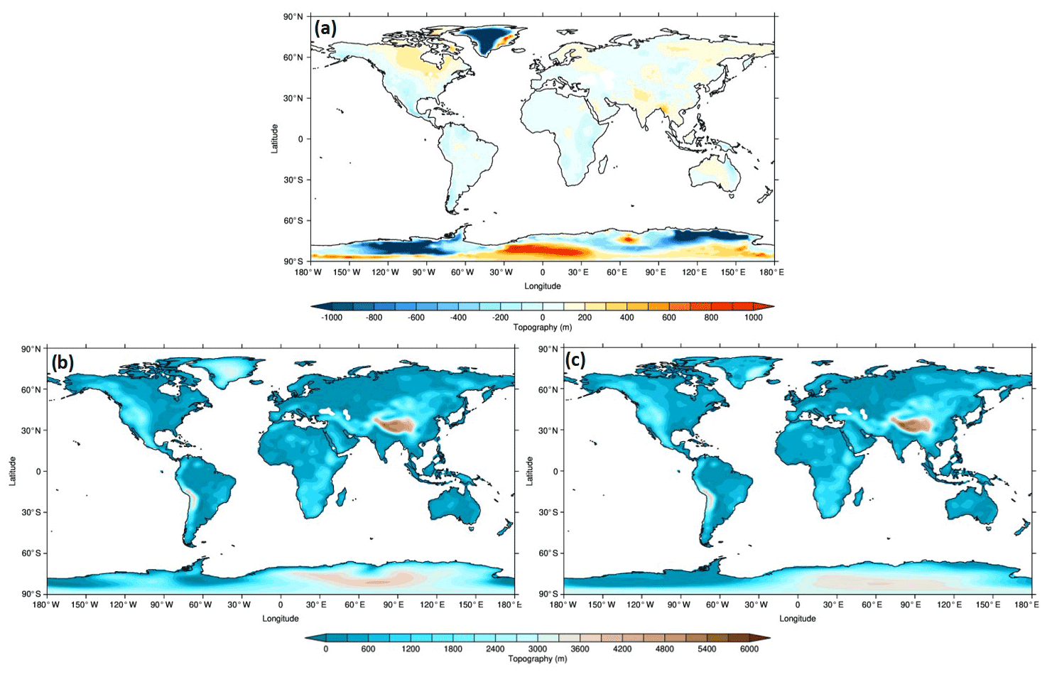
Figure 1 Changes to topography in HadGEM3 mPWP simulation: (a) PRISM4 anomaly, (b) original field used in the HadGEM3 piControl, (c) new field used in HadGEM3 mPWP, with smoothed topography over western Antarctica (final version, used in simulation).

Vegetation fractions (including urban, lakes and ice)

As part of its GL configuration, both the piControl and mPWP simulations used the community land surface model (JULES; see Best et al., 2011; Clark et al., 2011; Walters et al., 2019). In this land surface model, sub-grid-scale heterogeneity is represented by a tile approach (Essery et al., 2003), in which each grid box over land is divided into five vegetated plant functional types (PFTs): broadleaf trees (BLT), needle-leaved trees (NLT), temperate C₃ grass, tropical C₄ grass and shrubs. In addition to these, there are four non-vegetated PFTs: urban areas, inland water (or lakes), bare soil and land ice. This division of grid box into PFTs is consistent with both of the model's predecessors (see the Supplement). With the exception of the urban tile, which was kept as PI to be consistent with previous palaeoclimate simulations with this model (Williams et al., 2020b), all of these PFTs were modified in the mPWP simulation.

The US Geological Survey's PRISM4 (Dowsett et al., 2016) vegetation reconstruction from Salzmann et al. (2008) was used, provided as a megabiome reconstruction in PlioMIP2 (H16). This can be seen in Fig. 2, where there are 10 listed megabiomes corresponding to those used in Harrison and Prentice (2003): tropical forest, warm-temperate forest, savanna and dry woodland, grassland and dry shrubland, desert, temperate forest, boreal forest, tundra, dry tundra, and land ice.

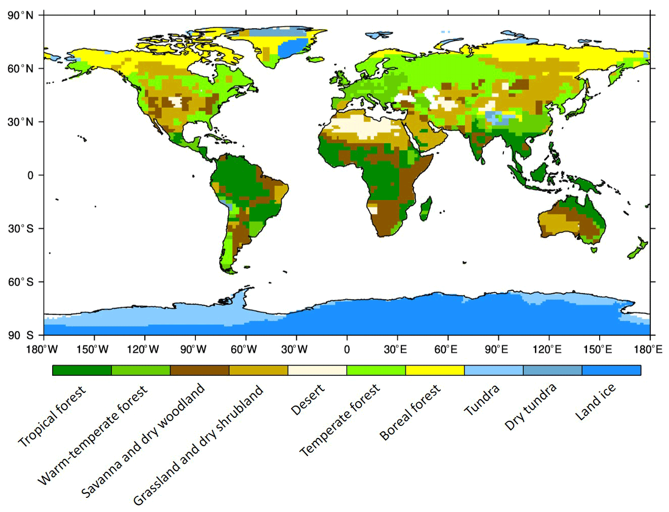
Figure 2 The 10 megabiomes from PlioMIP2 used to create the nine PFTs used in HadGEM3 mPWP simulation.

In order to translate the megabiomes from PRISM into the PFTs used by the model, a lookup table was required. Minimum and maximum bounds for each megabiome were firstly obtained, based on values from Crucifix et al. (2005), and then estimates were made for each PFT within these bounds by mapping the pre-industrial megabiomes onto the pre-industrial PFT in HadGEM3; the resulting lookup table is shown in the Supplement (Table S1). In this table, for example, each land grid point with the megabiome “Tropical forest” is divided amongst the model PFTs as 92 % BLT, 5 % bare soil, 2 % tropical C₄ grasses and 1 % shrubs. The resulting nine PFTs used in the mPWP simulation, as well as those from the original piControl, are shown in Fig. 3. The largest fractional increases, relative to the piControl, occur for broadleaf trees and needleleaf trees (18 % and 5 %, respectively; Fig. 3a and b), and the largest decreases occur for temperate C₃ grass and land ice (15 % and 5 %, respectively; Fig. 3c and i). In regions where there is no obvious match between the model's PFTs and the megabiomes, such as over western Antarctica (specified as tundra in the PRISM data), the closest match was provided; in this case, a mix of bare soil and shrubs.

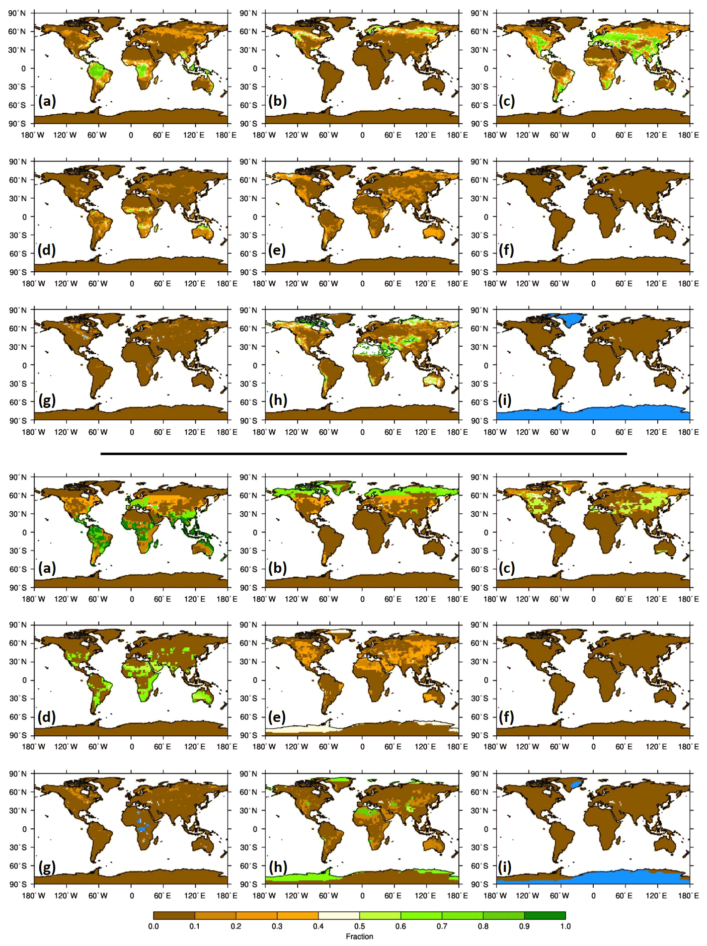
Figure 3 The nine PFTs used in HadGEM3. The top half of the figure (the first set of labelled panels) shows the piControl simulation, and the bottom half shows the mPWP simulation. Values in brackets show global mean differences (mPWP −  piControl), expressed as a percentage: (a) broadleaf trees (18 %), (b) needle-leaved trees (5 %), (c) temperate C₃ grass (−15 %), (d) tropical C₄ grass (6 %), (e) shrubs (3 %), (f) urban areas (no change), (g) inland water (1 %), (h) bare soil (−12 %), and (i) land ice (−5 %).

Vegetation functional types

Alongside the vegetation fractions, both the piControl and mPWP simulations included two monthly varying vegetation functional types, namely leaf area index (LAI) and canopy height, both of which are associated with each of the five vegetated PFTs. Given that no information was available from the PRISM vegetation reconstruction concerning these fields, two methods were used to create Pliocene LAI and canopy height. For LAI, a seasonally and latitudinally varying function was created from the zonal means of the piControl (Fig. 4) and used to build a new field for the Pliocene, for each month and each PFT (see Fig. 4b and c for an example of the original piControl and the Pliocene newly created field, respectively, both showing LAI for BLT during January). This is because LAI varies both in time (i.e. seasonally) and space in the piControl. Note that although LAI does go to zero in the piControl, this was not allowed in the mPWP simulation because the Pliocene does have some vegetation at high latitudes (see Fig. 3); these functions were therefore increased by x (where x is the mean of the 10 grid points containing the lowest LAI) such that there is never zero LAI. In contrast, canopy height in the piControl does not vary monthly and has little variation spatially, and therefore canopy height in the mPWP simulation is set to the global mean of the piControl simulation (see Fig. S2).

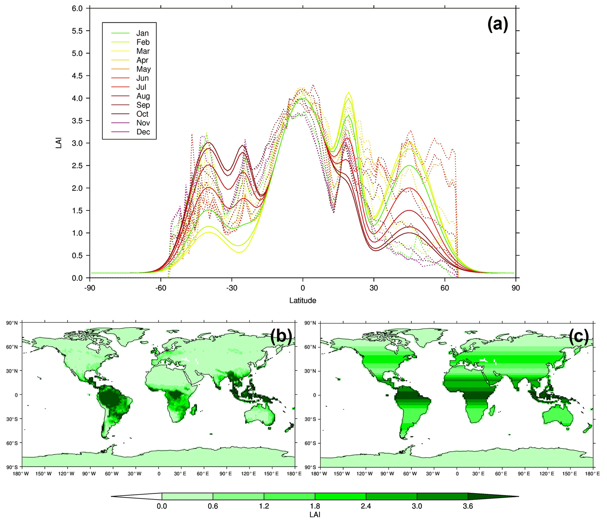
Figure 4 LAI used in HadGEM3 for an example PFT (broadleaf trees). (a) Function used to create LAI, where dashed lines show zonal mean from the piControl simulation and solid lines show seasonally and latitudinally varying function used in the mPWP simulation. (b) Example of functional types (broadleaf trees, January) used in the piControl simulation. (c) The same as (b) but for the mPWP simulation.

Soil properties and snow depth

Under newly created land ice based on the new Pliocene ice mask (i.e. in regions where there is no ice in the piControl simulation but ice in the mPWP simulation), soil parameters, soil dust properties and snow depth were set to be appropriate values for existing ice regions, i.e. whatever these values are under ice in the piControl simulation are applied to the newly created ice regions in the mPWP simulation.

Conversely, and more importantly in this context (as the Pliocene represents an overall removal of ice), under newly exposed land based on the new Pliocene ice mask (i.e. in regions where there is ice in the piControl simulation but no ice in the mPWP simulation, primarily over Greenland and western Antarctica), the dominant vegetation fractions in these regions were firstly identified from the newly created Pliocene vegetation. In this case, the dominant fractions were 40 % shrubs and 60 % bare soil. Following this, grid points containing this vegetation balance in the piControl were identified, and the soil parameters, soil dust properties and snow depth values at these points were averaged. This average value, for each of the above fields, was lastly inserted back into the mPWP simulation's newly exposed grid points; it is acknowledged that this introduces new dust emissions source regions, which may well impact the resulting Pliocene climate state.

Initial conditions

Oceanic initial conditions, such as ocean temperature and salinity, were derived from the mean equilibrium state of the piControl simulation. Some atmospheric initial conditions, such as those relating to the land surface (e.g. soil moisture and soil temperature at four levels of depth), used the same method as that applied to soil properties. These fields contain monthly varying values, therefore appropriate timings were considered, e.g. if the majority of grid points with the above balance were in the Northern Hemisphere, then initial conditions during Northern Hemisphere summer were used for newly exposed regions in Greenland (and likewise during Southern Hemisphere summer for newly exposed regions in Antarctica). For the soil temperature field and particularly at upper levels, this process resulted in sharp temperature gradients across western Antarctica; therefore, the field was spatially smoothed so that the gradients were more consistent with those in the piControl. Examples of the above soil-related fields are shown in Fig. 5 for an example month and vertical level. A complete list of the soil parameters and soil dust properties and how each were changed relative to the piControl are shown in the Supplement (Figs. S3 and S4, respectively).

Outside of the ice regions (i.e. outside Greenland and Antarctica), in the mPWP simulation the above soil-related fields were kept identical to those in the piControl simulation.

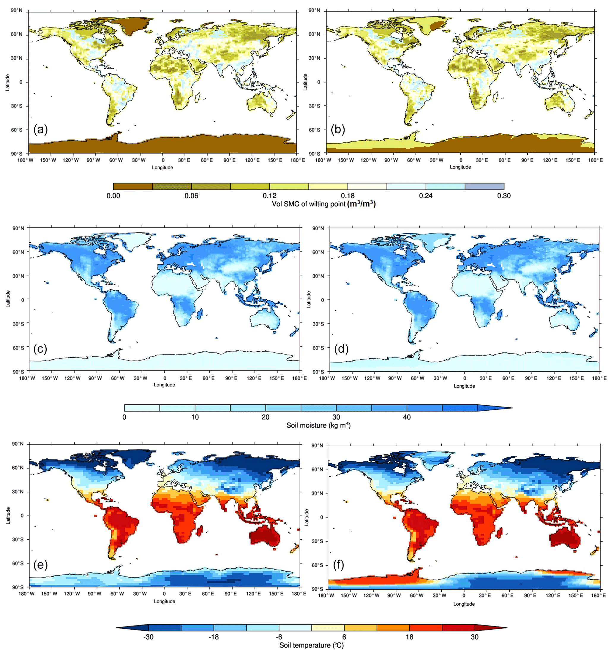
Figure 5 Example of soil-related fields used in HadGEM3 in the (a, c, e) piControl simulation and (b, d, f) mPWP simulation: (a, b) soil parameters (example shows volumetric soil moisture content at wilting point), (c, d) soil moisture (example shows January, top level) and (e, f) soil temperature (example shows January, top level). A complete list of fields is shown in Figs. S3 and S4.

2.3.3 Changes to input parameters

A small number of model input parameters were changed in the mPWP simulation to make the model more stable under the Pliocene boundary conditions. Firstly, a parameter governing the implicit solver for unstable atmospheric boundary layers was increased, and secondly three parameters for the treatment of canopy snow were made consistent between BLT and NLT. The same parameter changes will be included in the subsequent version of the physical model (GC4), in order to address occasional model failures that were seen following the release of GC3.1. They will be described in more detail in a GC4 model documentation paper; however, testing of those changes for GC4 has found that they have no detectable impact on model climatology.

2.4 Modified piControl simulation

Given that the official CMIP6 piControl simulation did not use the aforementioned model input parameter changes, a slightly modified version of this simulation was re-run (simulation ID: u-bq637), identical to the piControl other than including the parameter changes outlined in Sect. 2.3.3 (hereafter referred to as the piControl_mod simulation). This was run for 200 years, and the last 50-year climatology is considered here in Sects. 3 and 4.

3 Large-scale features of HadGEM3

3.1 Spin-up phase

Consistent with other palaeoclimate model experiments, the simulation should be run for as long as possible to allow the model to reach a state of equilibrium before the climatology is calculated over the last 30, 50 or 100 years (Lunt et al., 2017). With this model, however, running for thousands of years (especially important in obtaining oceanic equilibrium) was unfeasible given time and resource constraints. Therefore, by the end of the simulation there was a total of 576 years for the mPWP simulation, 526 of which are considered spin-up, and 50 of which form the final climatologies; this is approximately consistent with the 652 years of spin-up used by Menary et al. (2018).

Evolution of mPWP simulation

The HadGEM3 mPWP simulation was run in multiple parts, each starting from the endpoint of the last, and each introducing additional boundary conditions so as to gradually move from PI conditions to full Pliocene conditions. The mPWP simulation was started from the endpoint of the CMIP6 piControl simulation, specifically the last part of its spin-up phase (u-aq853), consistent with other CMIP6 HadGEM3 palaeoclimate simulations such as those of the mid-Holocene and Last Interglacial periods (see Williams et al., 2020b). The evolution of the mPWP simulation is shown in Fig. 6, where each stage is labelled and the resulting impact on the global mean 1.5 m air temperature is shown. The first part of the mPWP simulation (u-bq448) is a straight copy of the CMIP6 piControl production run (u-ar766), with no modifications other than increasing the atmospheric CO₂ to 400 ppmv; identical, therefore, to an E⁴⁰⁰ experiment following the naming convention of H16. This ran for ∼20 model years, before branching off to a new suite (u-br005) and introducing atmospheric ozone appropriate for Pliocene conditions and Pliocene orography (see Sect. 2.3.1 and 2.3.2, respectively). This ran for ∼60 model years, before branching off to a new suite (u-br871) and introducing a Pliocene-appropriate ice mask along with appropriate values for soil parameters, soil dust, soil moisture, soil temperatures and snow depth over these newly created ice regions (see Sect. 2.3.2); this, therefore would be the Eoi⁴⁰⁰ experiment following the naming convention of H16. It should be noted, however, that at this stage this naming convention is not strictly consistent with that used by H16 because they specify that orography, lakes and soils should be modified in unison, and therefore “o” here signifies changes to orography, bathymetry, land–sea mask, lakes and soils together. In contrast, at this stage of the simulation, most boundary conditions are consistent with the experimental design of H16, except vegetation, soils in non-ice regions and lakes. This ran for ∼280 model years (during which time the task of creating appropriate Pliocene vegetation was completed), before branching off to a new suite (u-bv241) and introducing a minor parameter change to allow inclusion of the Pliocene vegetation (see Sect. 2.3.3), as well as the full Pliocene vegetation fractions. This ran for a further ∼60 years to check the stability of the model in response to the vegetation change, before branching off to a new and final suite (u-bv963), in which the full Pliocene vegetation functional types were introduced. This ran for ∼150 years, with the final climatology (presented here in Sects 3 and 4) being taken from the last 50 years, i.e. allowing a 100-year buffer between the final update to the model and the actual results.

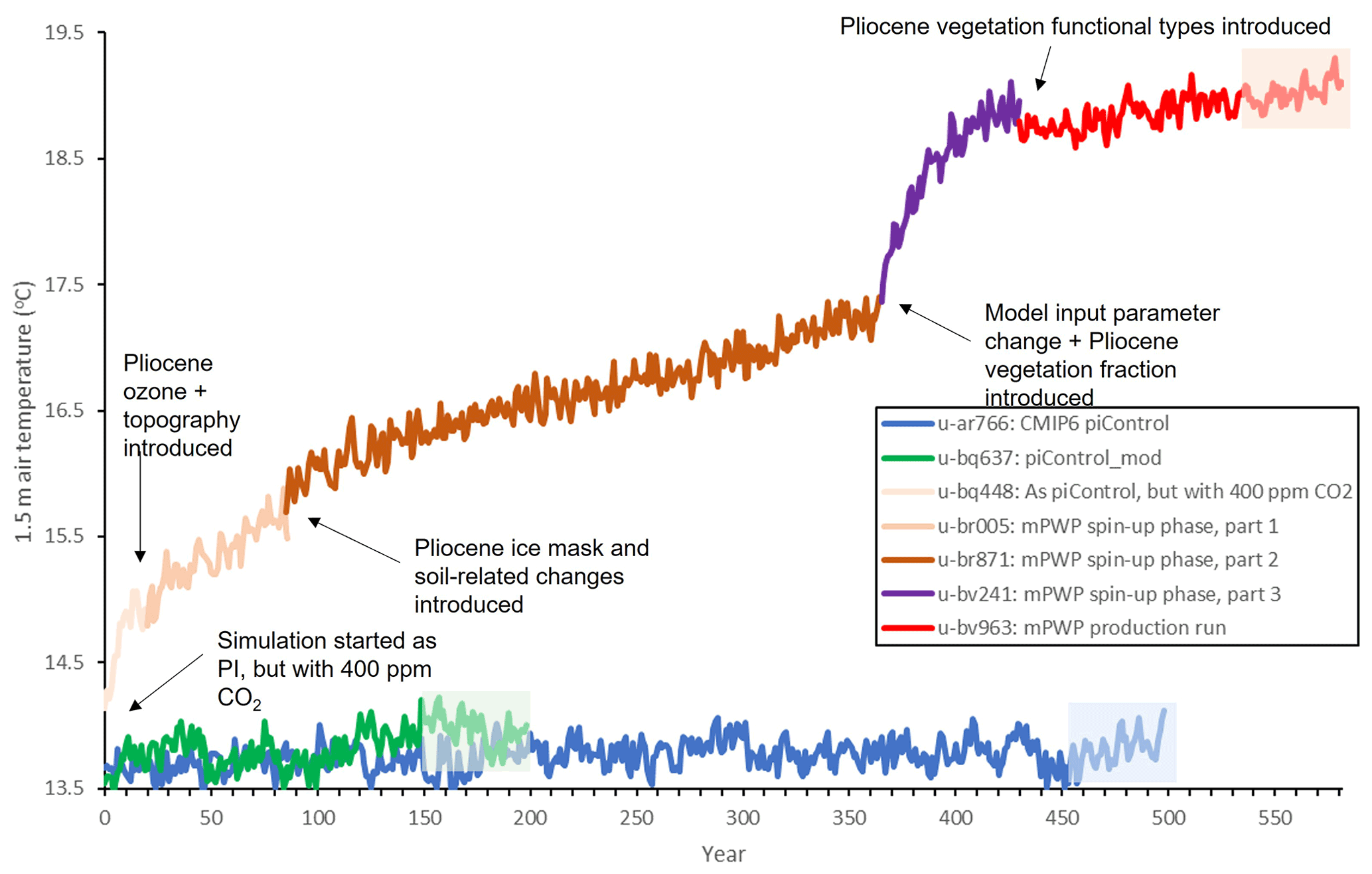
Figure 6 Annual global mean 1.5 m air temperature from the HadGEM3 mPWP spin-up phase and production run, as well as the CMIP6 piControl and the piControl_mod. Labels show introduction of each new Pliocene element. Climatologies discussed here are taken from final 50 years of each simulation (shown by shaded boxes). See Williams et al. (2020b) for the piControl spin-up phase that preceded these simulations.

As well as the various stages of the mPWP simulation, Fig. 6 also shows time series from the official ∼500-year CMIP6 piControl simulation (Kuhlbrodt et al., 2018; Menary et al., 2018) and the 200-year piControl_mod conducted here, and Fig. S7 shows climatologies of 1.5 m temperature and surface precipitation calculated over the last 50 years of each simulation. As the figures show, there is little or no difference between the two PI simulations (also suggested above in Sect. 2.3.3); using temperature as an example, over the last 50 years of the simulations there is a mean of 13.79 and 13.97 ^∘C for the piControl and piControl_mod, respectively, and a standard deviation of 0.13 ^∘C for both, further confirming the negligible impact of the model parameter change in the model climatology.

3.2 Atmospheric and oceanic equilibrium of the mPWP simulation

Concerning atmospheric equilibrium, Table 1 shows summary statistics for annual global mean 1.5 m air temperature and net top-of-atmosphere (TOA) radiation from the last 50 years of the mPWP simulation, compared to both the piControl and piControl_mod simulations; see Fig. 6 for the entire time series of Pliocene 1.5 m air temperature and Fig. S5 for the TOA radiation equivalent.

Table 1 Centennial trends (calculated via a linear regression) and climatology over the last 50 years of the simulations. A positive TOA imbalance indicates a net loss of energy from the Earth system.

Although the mPWP simulation is clearly warming considerably during the ∼500-year run (and especially when the Pliocene vegetation fraction is introduced), with trends of 0.77 ^∘C per century⁻¹, it levels off over the final 50 years, with trends of 0.34 ^∘C per century (Table 1). These values are higher than those considered by some (e.g. Menary et al., 2018) to be acceptable for equilibrium; however, given time and resource constraints it was not possible to run the simulation further. The spatial patterns of these trends, shown in Fig. S6, show the majority of the warming occurring over high-latitude regions in both hemispheres, related to the removal of the ice sheets and sea ice loss. By the end of the mPWP simulation, the mean TOA radiation balance is 0.88 W m⁻², significantly higher than either of the PI simulations, suggesting that the mPWP simulation is not yet in full atmospheric equilibrium. This TOA imbalance is reducing at a rate of 0.17 W m⁻² per century at the end of the simulation. A brief discussion of how the HadGEM3 mPWP simulation's atmospheric equilibrium compares to that of the other Hadley Centre models presented here (introduced in Sect. 4) is given in the Supplement (see Sect. S2 and Table S2).

When the mPWP simulation was stopped, the global annual mean 1.5 m temperature was approximately 19 ^∘C (Fig. 6). A Gregory plot (Gregory et al., 2004) of the evolution of TOA energy imbalance and surface temperature can indicate how much more warming the model may have experienced if it had been run to full equilibrium. The results of this analysis suggest the model would come to equilibrium ∼1.5 ^∘C higher (see Fig. S8) at 20.5 ^∘C, i.e. an anomaly relative to the pre-industrial period of 6.6 ^∘C. This is the case when the extrapolation is carried out on either of the final two parts of the simulation (in red and in purple in Fig. S8), suggesting that the introduction of the Pliocene vegetation functional types does not have a great impact on the final global mean temperature. However, this analysis is associated with some uncertainty, related to the interannual variability in temperature and TOA energy imbalance and to the fact that the linear extrapolation may not be appropriate if the feedbacks vary non-linearly (e.g. Knutti et al., 2015).

As an example of oceanic equilibrium, Table 1 also shows summary statistics for volume integral annual global mean ocean temperature and salinity from the end of the mPWP simulation compared to both the piControl and piControl_mod simulations; see Fig. S9 for the Pliocene time series. Ocean temperature is steadily increasing throughout the mPWP simulation, and likewise ocean salinity is steadily decreasing (Fig. S9). Freshwater fluxes to the ocean representing iceberg calving and ice sheet basal melt are calibrated for the piControl, as described in Sellar et al. (2020). These fluxes are calibrated to match the ice sheet surface mass balance (SMB) expected in the piControl, so that salinity drift is minimised. The Pliocene SMB is smaller than that in the piControl, and hence net flux of water to the ocean is positive, leading to the salinity drift. If computational resources allowed for a much longer Pliocene simulation, this ocean flux could be calibrated to Pliocene SMB once the temperature and SMB had stabilised or calculated iteratively. The long-term trends (Table 1) provide similar conclusions to those from the atmospheric trends, for example with centennial temperature trends of 0.21 ^∘C per century being much higher than the PI simulations (0.03 and 0.04 ^∘C per century for the piControl and piControl_mod, respectively). Although these values again do not meet the criteria of Menary et al. (2018) for oceanic equilibrium, given the aforementioned computational cost of this model it was not possible to run the simulations further; this is even more true in the ocean, which would require many thousands of years of model simulation to reach equilibrium. This compromise has been equally necessary for other computationally expensive palaeoclimate simulations (e.g. Williams et al., 2020b).

3.3 Simulation comparison: mPWP versus piControl_mod climatologies

Here the focus is on mean differences between the HadGEM3 mPWP simulation and its corresponding modified PI simulation, piControl_mod (Sect. 2.4). All of the following discussion and figures relate to climatologies calculated over the last 50 years of the simulations, and all of them are anomalies, i.e. Pliocene − PI. Annual and seasonal mean summer/winter 1.5 m air temperature (hereafter referred to as near-surface air temperature, SAT) anomalies are shown in Fig. 7. The annual global mean SAT anomaly for this 50-year climatology is 5.1 ^∘C. Warming relative to the PI is evident throughout the year and globally but more so over (i) landmasses (6.8 and 4.5 ^∘C for the annual mean SAT over land and ocean, respectively) and (ii) the Northern Hemisphere (8.5 and 6.3 ^∘C for annual mean SAT in the Northern Hemisphere and Southern Hemisphere extratropics; >45^∘, respectively). Warming is also evident over high latitudes (>60^∘) of both hemispheres (10.9 and 8.5 ^∘C for the Northern Hemisphere and Southern Hemisphere, respectively, and exceeding 12 ^∘C in some places). These particular metrics were chosen to be consistent with those used by H20 (see Sect. 4.2). Over the tropics (20^∘ N–20^∘ S) the amount of warming is less than at higher latitudes, but the Pliocene is still much warmer than the PI with annual mean SAT anomalies of 4.6 and 3.7 ^∘C when averaged over tropical land and ocean, respectively. This global and regional warming is consistent with, albeit slightly warmer than, other work, namely the results from PlioMIP1 (Haywood et al., 2013) and PlioMIP2 (see Sect. 4.2). The majority of the annual mean warming (Fig. 7a) in Northern Hemisphere high latitudes is accounted for during that hemisphere's winter (December–February, DJF) with a mean warming of 15 ^∘C (Fig. 7b), and likewise the majority of the annual mean warming in Southern Hemisphere high latitudes is accounted for during that hemisphere's winter (June–August, JJA) with a mean warming of 10.6 ^∘C (Fig. 7c). If the entire hemisphere rather than >60^∘ is considered, then this greater winter contribution to the annual mean is still true, although the contribution is lower (e.g. 5.6, 6.1, and 5.4 ^∘C for the annual, DJF and JJA means, respectively, in the Northern Hemisphere).

The regions of polar SAT increases and seasonal variation are likely explained by the changes in sea ice shown in Fig. 8 (for the absolute values in sea ice fraction, see Fig. S10). Reductions in sea ice are shown throughout the year in both hemispheres, consistent with previous work (e.g. Cronin et al., 1993; Howell et al., 2016; Moran et al., 2006; Polyak et al., 2010). Here, although a reduction in sea ice (of up to 70 %) is evident throughout the year in either hemisphere, at the seasonal timescale the largest loss (exceeding 70 % in some places, such as the polar Arctic and Antarctic) is seen during each hemisphere's winter (Fig. 8a and d). The regions and timings of maximum warming (Fig. 7b–c) correspond well to the regions and timings of maximum sea ice loss, implying a role for the sea ice–albedo feedback. When sea ice area is averaged over each hemisphere (Fig. 8e), the Northern Hemisphere is clearly losing more sea ice in the mPWP simulation (relative to the piControl_mod) than the Southern Hemisphere. However, the amount of loss in the Southern Hemisphere is steadily increasing during the last 50 years of the mPWP simulation, suggesting that had the model been allowed to run to full equilibrium, the difference between the hemispheres would be reduced.

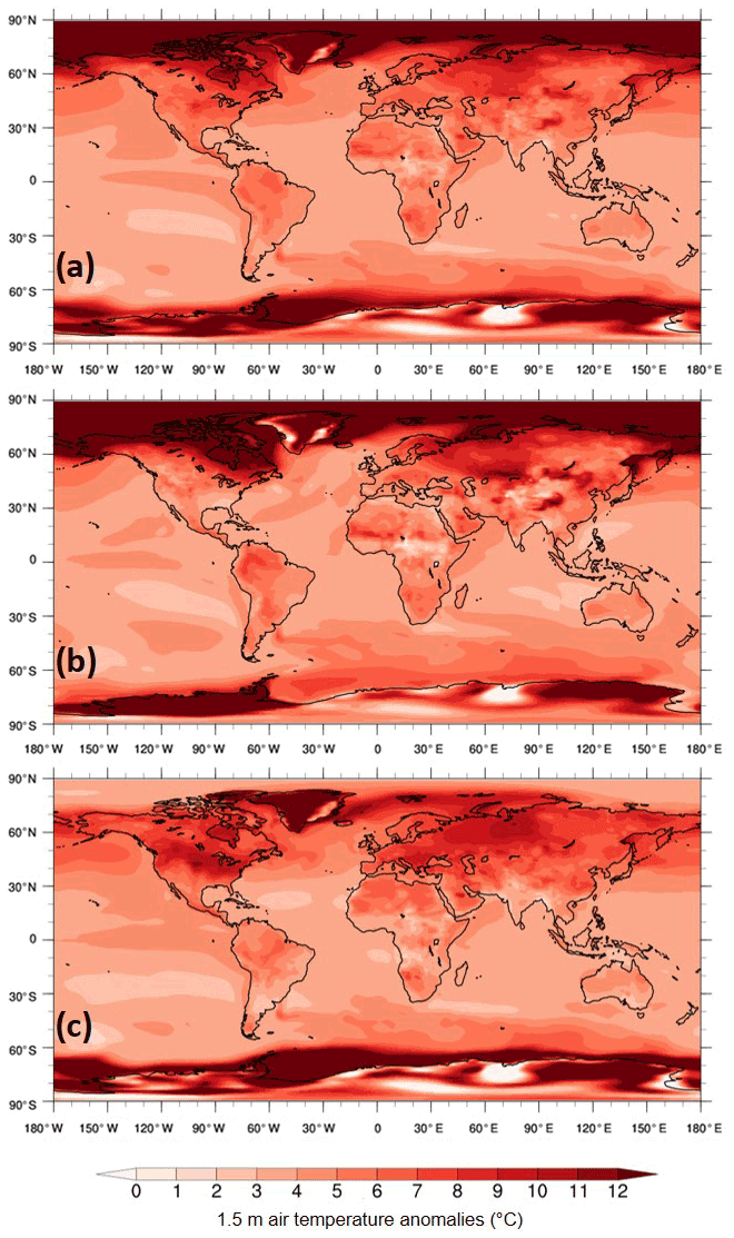
Figure 7 The 1.5 m air temperature climatology differences (mPWP − piControl_mod) from HadGEM3: (a) annual, (b) DJF and (c) JJA.

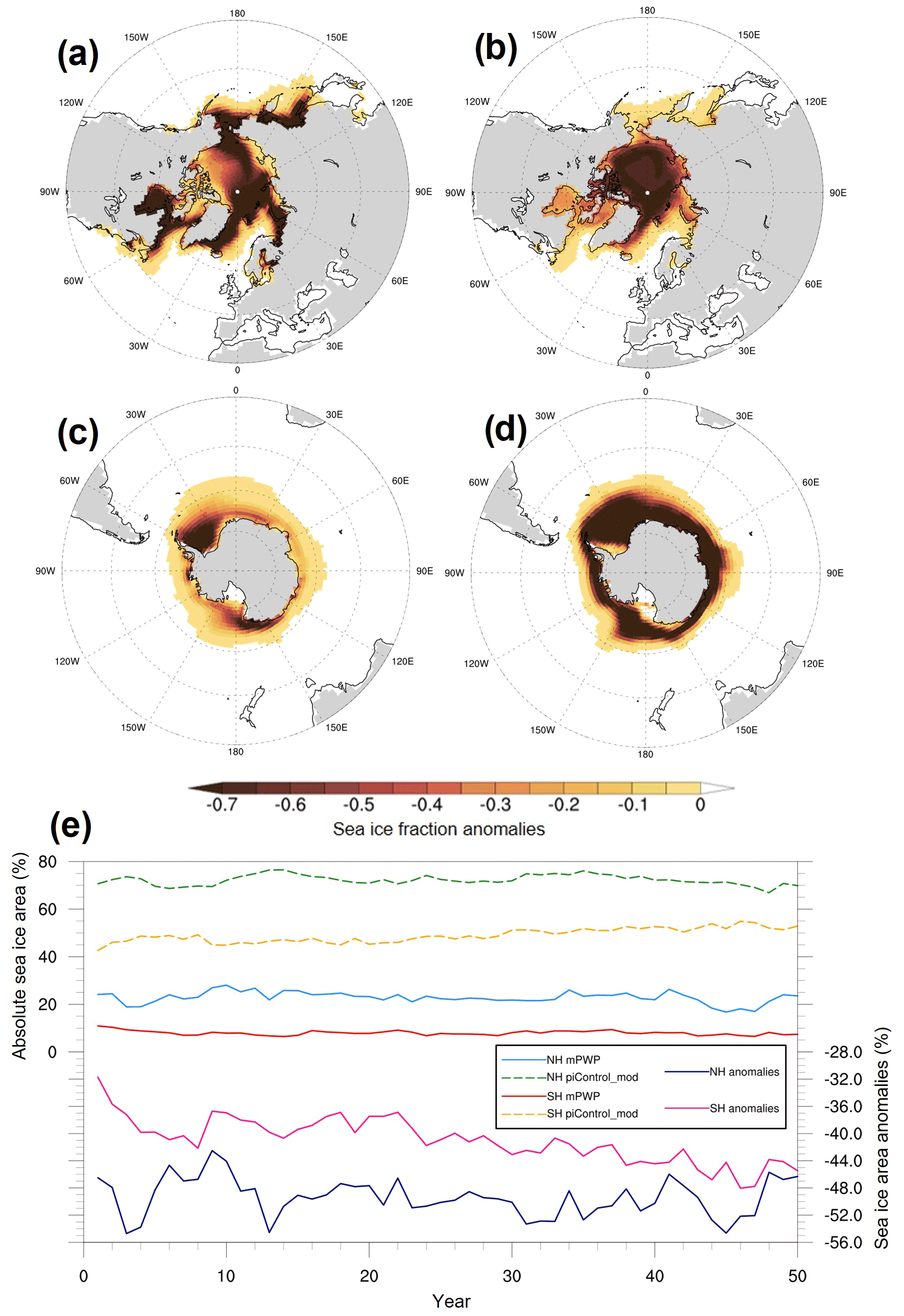
Figure 8 Sea ice fraction climatology differences (mPWP − piControl_mod) from HadGEM3: (a) Northern Hemisphere DJF, (b) Northern Hemisphere JJA, (c) Southern Hemisphere DJF, (d) Southern Hemisphere JJA and (e) mean sea ice area (both absolute values and differences) averaged over either hemisphere.

Annual and seasonal mean surface daily precipitation anomalies are shown in Fig. 9. The annual global mean precipitation anomaly for this 50-year climatology is 0.34 mm d⁻¹. In addition to the precipitation increases at high latitudes at the annual timescale (Fig. 9a), which are again mostly accounted for by changes during the Northern Hemisphere's and Southern Hemisphere's winters (Fig. 9b and c, respectively), the largest change relative to the PI is a northward displacement of the Intertropical Convergence Zone. All timescales are showing wetter conditions over oceans to the north of the Equator and drier conditions over oceans to the south of the Equator. This is similar to work by Li et al. (2018), who suggested a poleward movement of Northern Hemisphere monsoon precipitation in PlioMIP1. There is also a noticeable enhancement of monsoon systems such as the East Asian and West African monsoons, consistent with previous work (e.g. Zhang et al., 2013, 2016). In some places, these changes exceed ∼2 mm d⁻¹, geographically consistent with (albeit again much higher than) other work, such as the multi-model ensemble mean (MME) from PlioMIP2 models where increases rarely exceed ∼1.2 mm d⁻¹ (see Sect. 4.2). These changes, and indeed the temperature changes over Northern Hemisphere landmasses, may be associated with changes to the total cloud cover shown in Fig. 10. Although the changes are small at the annual timescale (Fig. 10a), during Northern Hemisphere winter (Fig. 10b) there is a noticeable increase in cloud cover (of ∼10 %) over high-latitude regions corresponding to the increases in precipitation. Likewise, during Northern Hemisphere summer (Fig. 10c) there is a large reduction (over 20 % in places) in cloud cover, especially over Northern Hemisphere landmasses; these regions, such as Europe and northern Asia, correspond well to the areas of decreased precipitation and increased temperature.

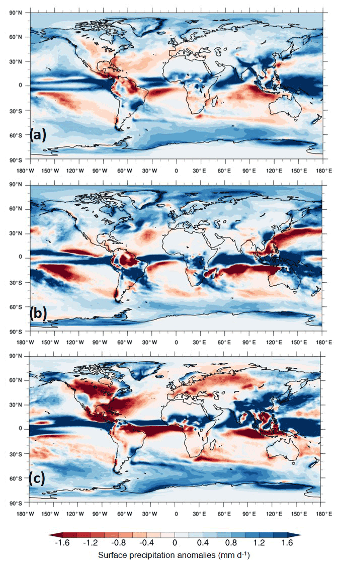
Figure 9 Surface precipitation climatology differences (mPWP − piControl_mod) from HadGEM3: (a) annual, (b) DJF and (c) JJA.

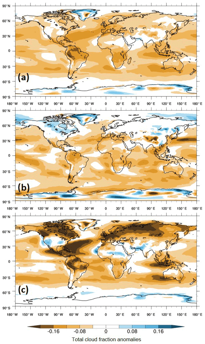
Figure 10 Total cloud fraction climatology differences (mPWP − piControl_mod) from HadGEM3: (a) annual, (b) DJF and (c) JJA.

4 Comparison of HadGEM3 with other models and proxy data

4.1 Model–model and model–data comparison: different generations of UK model versus proxy data

Here the focus is on mean SST differences between different generations of the UK's physical climate model, starting with three Pliocene simulations using the original fully coupled climate model HadCM3, then a simulation from the more recent HadGEM2 and finally the mPWP simulation from HadGEM3. See the Supplement for the details of these older models. For HadCM3, three separate Pliocene simulations (and corresponding PIs) are used; the first two were conducted by Lunt et al. (2012) and Bragg et al. (2012) and are referred to as HadCM3-PRISM2 and HadCM3-PlioMIP1, respectively (see Table 2). This is to distinguish them from a third version of the same model included in PlioMIP2, referred to here as HadCM3-PlioMIP2.

Table 2 Different generations of the UK physical climate model used here and their involvement with PlioMIP.

Multi-proxy SST data from the KM5c interglacial compiled by McClymont et al. (2020) were used for comparative purposes. Here, they focus on a narrow time slice from 3.195 to 3.215 Ma and compile the SST data from two proxies: an alkenone-derived U${}_{\mathrm{37}}^{{\mathrm{K}}^{\prime }}$ index (Prahl and Wakeham, 1987) and foraminifera calcite $\mathrm{Mg}/\mathrm{Ca}$ (Delaney et al., 1985), with the resulting data comprising the PlioVAR synthesis and covering 32 locations between 46^∘ S–69^∘ N (McClymont et al., 2020).

Maps of annual mean SST anomalies from the simulations, overlaid with the proxy data, are shown in Fig. 11 and summary statistics are shown in Table 3.

Figure 11 Annual mean SST differences (Pliocene − PI) from different generations of the UK's physical climate model: (a) HadCM3-PRISM2, (b) HadCM3-PlioMIP1, (c) HadCM3-PlioMIP2, (d) HadGEM2 and (e) HadGEM3. Background gridded data show model simulations, and filled circles show SST proxy data from McClymont et al. (2020).

Table 3 Global annual mean SST anomalies from Pliocene simulations using different generations of the UK's physical climate model and RMSE values between simulations and SST proxy data from McClymont et al. (2020).

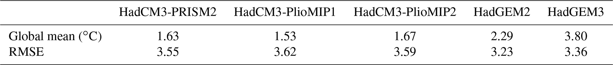
The global annual SST anomaly for HadGEM3 is 3.8 ^∘C, followed by HadGEM2 at 2.3 ^∘C and 1.7, 1.5, and 1.6 ^∘C for the three HadCM3 simulations (starting with the most recent, HadCM3-PlioMIP2; see Table 3). Comparing the newest model (HadGEM3) with the oldest model (HadCM3-PRISM2), which have an anomaly of 3.8 and 1.6 ^∘C, respectively, clearly the most recent generation shows a much warmer Pliocene.

Comparing an earlier generation of the model with a later generation that has identical boundary conditions (HadCM3-PlioMIP1 and HadGEM2, respectively; Fig. 11b and d), aside from the greater overall warming (2.3 ^∘C in HadGEM2 versus 1.5 ^∘C in HadCM3-PlioMIP1) already discussed above, the main spatial patterns of warming are similar, with both showing the greatest warming over the Labrador Sea and the northwestern Pacific and HadGEM2 showing greater polar amplification overall. In part thanks to this high-latitude warming, root-mean-squared error (RMSE) values are 3.2 and 3.6 ^∘C for HadGEM2 and HadCM3-PlioMIP1, respectively, showing a greater agreement between the proxy data and HadGEM2 (Table 3).

Likewise, comparing the other older model with the most recent (HadCM3-PlioMIP2 and HadGEM3, respectively; Fig. 11c and e), the spatial patterns of warming differ more widely, with HadGEM3 showing widespread Northern Hemisphere high-latitude warming that is not shown by HadCM3-PlioMIP2 at all (other than in the Labrador Sea). HadGEM3, and indeed HadGEM2, are displaying a greater extent of polar amplification in both hemispheres (Fig. 11d–e). As the warmest model, HadGEM3 (RMSE=3.4 ^∘C) shows less agreement with the proxy data than HadGEM2 (RMSE=3.2 ^∘C), likely because it is so warm that the discrepancy with the colder proxy data locations (such as in the Indian Ocean, near New Zealand or off equatorial Africa) is greater (Fig. 11e). This is in spite of the fact that in the warmer proxy data locations (such as in the North Atlantic and Arctic) HadGEM3 is closer to the proxy data. In these regions, the earlier versions of the model (Fig. 11a–c) do not even capture the sign of change and show a weak cooling, in stark contrast to the proxy data, that neither HadGEM2 nor HadGEM3 display (Fig. 11d–e). Where proxy data suggest colder conditions, again none of the models capture the sign of change and all show widespread warming, and this is most evident in HadGEM3 because of its particularly strong warming. The fact that all of the HadCM3 simulations show several regions of cooling and have a higher RMSE than the most recent versions suggests that this early model might be too cold. In contrast, the fact that HadGEM3 has a higher RMSE than HadGEM2 suggests that, despite involving significant model development (see Williams et al., 2020b, for a summary), concerning Pliocene climate HadGEM3 may actually be too warm. Therefore, whilst model development appears to have improved the model's agreement with proxy data since earlier versions of the model, this only appears to be true up to a certain point; the “sweet spot” appears to be HadGEM2. Moreover, given the aforementioned point about the mPWP simulation not being in full equilibrium and being ∼1.5 ^∘C warmer if it had been (see Sect. 3.1.2), it is likely that both the SST anomaly and the RMSE values would be higher when in equilibrium, and therefore the performance against proxy data may be lower than indicated here.

4.2 Model–model comparison: HadGEM3 versus PlioMIP2 models

Finally, the focus here is on mean differences, again considering SAT and precipitation anomalies, between the mPWP simulation from HadGEM3 and the Pliocene simulations from all other available models included in PlioMIP2 (Table 4).

Table 4 Climate models included here from PlioMIP2 (see Haywood et al., 2020 for each model's reference).

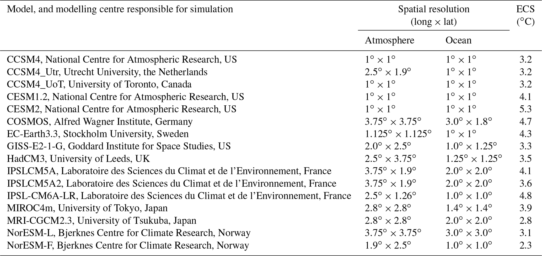
A number of different metrics of SAT are shown in Fig. 12 for each of the models, as well as the MME; the panels shown here are updated versions of those shown in H20 but now including HadGEM3. It should be noted that, consistent with H20, the models are listed according to their published ECS, with the highest ECS listed first (see Table 4). HadGEM3 has an ECS of 5.5 K (Andrews et al., 2019), compared to the second highest model (CESM2) with an ECS of 5.3 K (H20). If, however, all available models within CMIP6 (i.e. not just those having conducted Pliocene simulations) are considered, then HadGEM3 has the second highest ECS, just below that of CanESM5 with an ECS of 5.6 K (Zelinka et al., 2020).

Figure 12 SAT from Pliocene simulations from HadGEM3 and all other models in PlioMIP2: (a) global annual mean SAT (top panel) and anomalies (bottom panel), (b) extratropical (±45^∘) annual mean SAT anomalies (top panel) and ratio (i.e. >45^∘ N divided by <45^∘ S) between them (bottom panel), (c) land and ocean annual mean SAT anomalies, averaged globally (top panel) and between 20^∘ N and 20^∘ S (bottom panel), and (d) annual mean SAT polar amplification, i.e. SAT poleward of 60^∘ divided by global mean, for each hemisphere, where the red line shows a ratio of 1 (i.e. no polar amplification). Figures reproduced and adapted from Haywood et al. (2020).

As mentioned above (Sect. 3.2), the global annual SAT anomaly by the end of the mPWP simulation is 5.1 ^∘C, making HadGEM3 one of the warmest models in PlioMIP2 and second only to CESM2 (H20). This is true both in terms of its anomaly and its mean Pliocene SAT (19 ^∘C); this is only lagging behind the warmest model by 0.2 and 0.3 ^∘C for the anomalous and mean SAT, respectively (Fig. 12a). HadGEM3 is much warmer than earlier global annual mean temperature estimates (e.g. Haywood and Valdes, 2004), and the range given by models included in PlioMIP1 (1.8 to 3.6 ^∘C; see Haywood et al., 2013) and PlioMIP2 (1.7 to 5.2 ^∘C, see H20). The impact of including HadGEM3 amongst the models is to increase the MME anomaly by 0.1 ^∘C, from 3.2 to 3.3 ^∘C. Interestingly, the HadGEM3 piControl_mod simulation does not present the warmest absolute PI compared to the other models, coming fourth in the list, suggesting that HadGEM3 is more sensitive to the Pliocene boundary conditions rather than being a generally warmer model overall.

Concerning annual global mean precipitation (Fig. 13a), as mentioned above the precipitation anomaly by the end of the simulation is 0.34 mm d⁻¹, making HadGEM3 not only one of the warmest models in PlioMIP2 but also one of the wettest (consistent with current understanding, as global precipitation is generally a function of global temperature). The range of anomalies across all models during PlioMIP1 was 0.09 to 0.18 mm d⁻¹ (Haywood et al., 2013), during PlioMIP2 it was 0.07 to 0.37 mm d⁻¹ (with the higher values being attributed to the models being more sensitive to the updated PRISM4 boundary conditions), and the PlioMIP2 ensemble mean was 0.19 mm d⁻¹ (H20). Concerning the mean, it is the wettest model in terms of both its mPWP (3.49 mm d⁻¹) and piControl_mod (3.15 mm d⁻¹) simulations, and both of these are much higher than the MME (3.06 and 2.86 mm d⁻¹ for the Pliocene and PI simulations, respectively). The fact that both the HadGEM3 mPWP and piControl_mod simulations are not only the wettest but also closer together in terms of mean precipitation, means that if the anomaly is considered (Fig. 13b) HadGEM3 does not quite show the greatest change relative to the PI; an anomaly of 0.34 mm d⁻¹ makes it second only to CCSM4-Utr (at 0.37 mm d⁻¹). The impact of including HadGEM3 amongst the other PlioMIP2 models is to again slightly increase the MME anomaly, from 0.19 mm d⁻¹ as reported by H20 to 0.2 mm d ⁻¹ here.

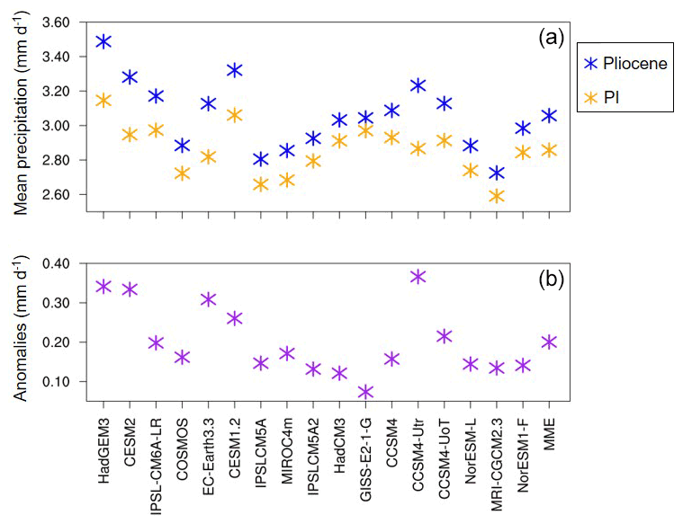
Figure 13 Global annual mean surface precipitation (a) and anomalies (b) from the HadGEM3 mPWP simulation and all other models in PlioMIP2, as well as multi-model ensemble mean (MME). Figure reproduced and adapted from Haywood et al. (2020).

If the hydrological sensitivity (i.e. the relationship between global annual mean precipitation anomalies and SAT anomalies) of the models is considered, then in line with current understanding (e.g. Pendergrass and Hartmann, 2014) there is a clear linear relationship shown by most of the models, with Pliocene increases in precipitation increasing in line with SAT increases (Fig. 14). This relationship is not entirely linear, however, with the aforementioned result being shown again here, i.e. although the HadGEM3 mPWP simulation is the second warmest of all models in PlioMIP2, it is not the wettest, suggesting that although the model is highly sensitive to the Pliocene forcings in terms of its temperature response, it may be less sensitive in terms of its hydrological response.

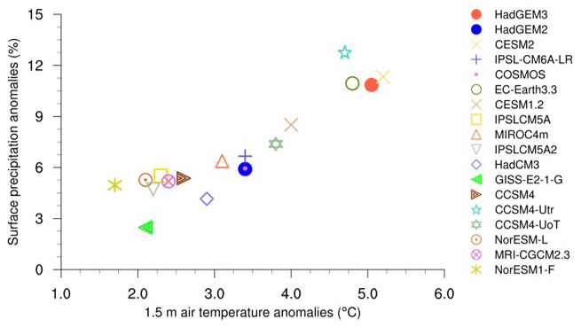
Figure 14 Global annual mean surface precipitation anomalies (expressed as a percentage) versus global annual mean SAT from HadGEM3 mPWP simulation, HadGEM2 and all other models in PlioMIP2.

Returning to SAT and if only extratropical warming (separated by hemisphere, above or below 45^∘ N or S) is considered, then HadGEM3 agrees with the other 11 models (out of 16) that H20 identified as showing enhanced Northern Hemisphere warming, relative to the Southern Hemisphere (Fig. 12b, top panel). In the Northern Hemisphere, HadGEM3 is again one of the warmest models and (at 8.46 ^∘C) is considerably warmer than most other models and the MME; this, with the inclusion of HadGEM3, has now increased from the 5.5 ^∘C reported in H20 to 5.7 ^∘C here. However, in the Southern Hemisphere HadGEM3 is closer to many of the other models, although it is still in the top 33 % of them and with a warming of 6.3 ^∘C is much closer to the MME of 5.1 ^∘C (Fig. 12b, top panel). This is further demonstrated by Fig. 12b (bottom panel), showing the ratio of warming between the hemispheres (calculated by dividing the Northern Hemisphere warming by the Southern Hemisphere warming), where HadGEM3 is giving a ratio of 1.34, which is again close to many of the other models and the MME (1.17). Considering land–sea temperature contrasts (Fig. 12c), as H20 state all of the PlioMIP2 models show more warming over land both globally and across the tropics (defined as 20^∘ N–20^∘ S), and HadGEM3 is no exception. Indeed, over either land or sea, HadGEM3 is the second warmest globally and warmest across the tropics, and the inclusion of this model increases the MME by 0.1–0.14 ^∘C depending on whether land or sea warming is considered.

HadGEM3 is one of the largest outliers regardless of metric; however, concerning polar amplification this is not the case. Here, as in H20, polar amplification is defined as the ratio of SAT increases poleward of 60^∘ divided by the global mean SAT increases (Smith et al., 2019), calculated independently for each hemisphere. Despite the HadGEM3 mPWP simulation qualitatively showing considerable amplification at both annual and seasonal timescales (Fig. 7), when quantitatively compared with all other PlioMIP2 models, HadGEM3, whilst still having amplification >1 (i.e. that there is some amplification of warming around the poles), nevertheless shows considerably less amplification in both hemispheres and is also lower than the MME in both hemispheres (Fig. 12d). Of all the models, HadGEM3 comes fourth-to-last for Northern Hemisphere amplification and last for Southern Hemisphere amplification, and its inclusion with the other models reduces the MME ratio by approximately 0.01 and 0.04 for the Northern Hemisphere and Southern Hemisphere, respectively. This is consistent with the conclusions of H20, who note a weak relationship between ECS and amplification; they observe that models with a lower ECS tend to display higher PA, whereas the opposite appears to be shown here, i.e. HadGEM3, with one of the highest ECS, displays one of the lowest amounts of amplification. The amplification for all the models, as well as the MME, can be seen graphically in Fig. S11, where at first glance HadGEM3 would appear to show one of the largest amounts of amplification. However, consistent with the observation by H20, this is because the model shows more warming in the tropics (relative to the other models) rather than less warming at high latitudes.

Lastly, concerning SST anomalies the HadGEM3 mPWP simulation is warmer than most other models in PlioMIP2 (Fig. 15). When simulated SST is compared to the proxy data from McClymont et al. (2020), if the models are ranked according to RMSE then the HadGEM3 mPWP simulation (RMSE=3.4 ^∘C; see Table 3) ranks approximately halfway amongst them. There appears to be a weak relationship between the warmth of the model and agreement with proxy data, with some of the other warm models (e.g. CESM2, the warmest model) showing less agreement (RMSE=3.5 ^∘C) with the proxy data than HadGEM3; however, this is not always true, such as the case of the CCSM4-Utr, which is also comparatively warm but shows a slightly better agreement (RMSE=3.3 ^∘C) with the proxy data. It is likely that the location of the proxy data is important, as the best agreement comes from the MME (RMSE=3.1 ^∘C), which shows warm SST anomalies over the North Atlantic and Arctic (there in better agreement with the proxy data) but less warming relative to HadGEM3 and CESM2 in the Southern Hemisphere (better in agreement with the proxy data in, e.g. the Indian Ocean).

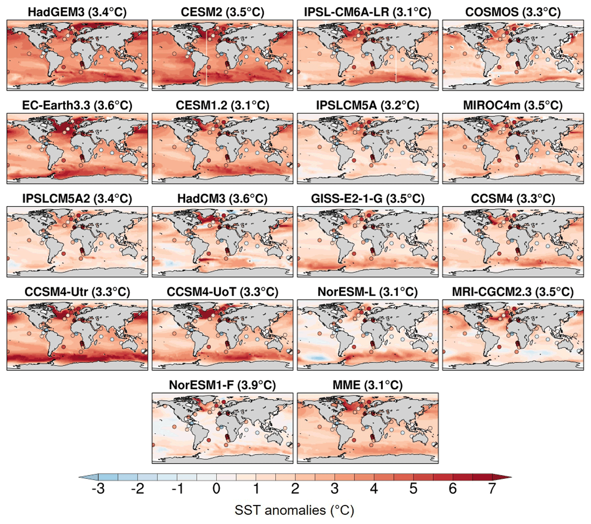
Figure 15 SST climatology differences (Pliocene − PI) from HadGEM3 mPWP simulation and all other models in PlioMIP2, as well as multi-model ensemble mean (MME). Numbers in brackets show RMSE scores when compared proxy data from McClymont et al. (2020).

It is likely that much of the greater warming in the HadGEM3 mPWP simulation, relative to the other models, can be attributed to the relatively high ECS of this model. Figure 16 shows model ECS against simulated Pliocene warming for all available models (see Table 4 for individual ECS values). Also shown in Fig. 16 is the Earth system sensitivity (ESS), which for the Pliocene can be taken as the global mean temperature scaled by the CO₂ forcing for 560 ppmv compared with 400 ppmv. This is because the temperature change due to the modified orography is small, and so the Pliocene warming relative to pre-industrial values is due to the CO₂ forcing and associated feedbacks due to vegetation and ice sheets, which can be interpreted as ESS (Lunt et al., 2010). Therefore, a plot of Pliocene global mean warming against ECS will be identical to a plot of ESS against ECS, but with different values on the y axis. There is a clear linear relationship between ECS and global mean warming (or ESS), with the two models showing the highest ECS also having the highest Pliocene warming or ESS (HadGEM3 and CESM2). Despite some outliers, such as CCSM4-Utr with a relatively high global mean temperature anomaly but a relatively low ECS, this would suggest that for most models Pliocene temperature anomalies (and ESS) are increasing in line with ECS.

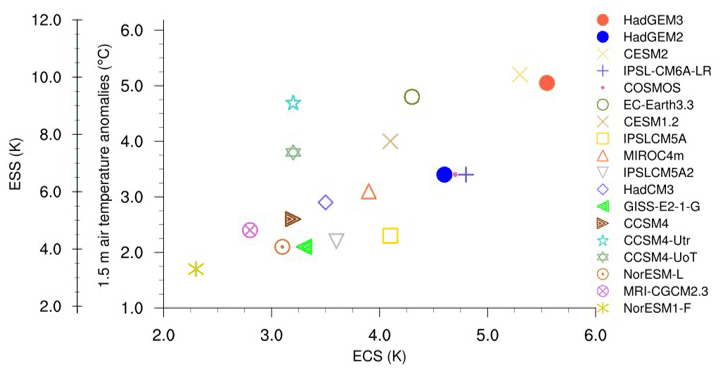
Figure 16 Global annual mean SAT anomalies versus both ESS (first y axis) and ECS from HadGEM3 mPWP simulation, HadGEM2 and all other models in PlioMIP2. The ESS axis is calculated by multiplying the global annual mean SAT anomaly by $\log (\mathrm{560}/\mathrm{280})/\log (\mathrm{400}/\mathrm{280})$, i.e. by 1.94, meaning the axis here goes from 1.94 to 11.64 K; for simplicity, this has been rounded up to 2–12 K.

5 Summary and conclusions

This study has introduced the mid-Pliocene simulation using the latest version of the UK's physical climate model, HadGEM3-GC31-LL, presented a new experimental design, and conducted a model–model and model–data comparison. This study is novel, being the first time this version of the UK model has been run this far back in time; only two other palaeoclimate simulations using this model have thus far been conducted, comprising the UK's contribution to CMIP6/PMIP4, and both of these were more recent, Quaternary simulations (Williams et al., 2020b).

The mPWP simulation mostly followed the experimental design defined in H16, with the exception being the exclusion of a Pliocene LSM and Pliocene soils. Both of these were kept the same as PI. All other boundary conditions, including CO₂, orography, ice mask, lakes, vegetation fractions and vegetation functional types followed the protocol of H16 and were incrementally implemented to be Pliocene based on the PRISM4 dataset. A minor model parameter change was included to increase the model's stability in light of the strong Pliocene forcing, and thus a corresponding PI simulation was also run for comparison purposes. The mPWP simulation was run for 567 years in total, during which atmospheric and oceanic equilibrium were assessed. Although not meeting the criteria used to determine equilibrium in other palaeoclimate simulations, especially concerning oceanic equilibrium, due to computational restrictions it was not possible to run this model for the thousands of years required to achieve this.

The results presented here are divided into three sections: (i) a simulation comparison, in which the mPWP simulation is compared to its corresponding piControl_mod simulation (Sect. 3.2); (ii) a model–model and model–data comparison, in which the most recent mPWP simulation is compared to Pliocene simulations from previous versions of the same model, all assessed against proxy data (Sect. 4.1); and (iii) a model–model comparison, in which the most recent mPWP simulation is compared to other models (Sect. 4.2).

For the first comparison, the mPWP simulation behaves in line with current understanding and previous work (e.g. Haywood et al., 2013, H20), showing a warmer and wetter world relative to the PI, with the greatest warming occurring over the poles. This polar warming, which can be attributed to a loss in sea ice and changes in clouds, and the changes to precipitation (such as an enhancement of monsoon systems) all agree with the expected response and previous work (e.g. Cronin et al., 1993; Howell et al., 2016; Li et al., 2018; Moran et al., 2006; Polyak et al., 2010; Zhang et al., 2013, 2016). For the second comparison, there is a clear increase in global temperatures (as measured by SST) as the model develops through time, beginning with the early Pliocene simulations using HadCM3 (Lunt et al., 2012; Bragg et al., 2012), through HadGEM2 (Tindall and Haywood, 2020) and up to the most recent mPWP simulation from HadGEM3 presented here. Up to a point, this warming results in a better agreement with available proxy data. However, just as the earlier HadCM3 simulations appear to be too cold relative to some proxy data, the most recent mPWP simulation from HadGEM3 appears to be too warm; the “sweet spot” appears to be the previous generation of the model, HadGEM2. This would be even more the case had the mPWP simulation been allowed to run to full equilibrium, and it is suggested that the final global mean surface temperature could have been approximately 1.5 ^∘C higher if this were the case. For the third comparison, the above conclusion that HadGEM3 is too warm is further suggested by the fact that it is one of the warmest and wettest models (even at its current state of equilibrium) in all of PlioMIP2 (H20), and this is true over either land or sea and especially in the Northern Hemisphere. When compared to proxy SST data, HadGEM2 ranks approximately halfway amongst the models and is much too warm in certain locations, such as the Indian Ocean. However, the conclusion that the model is too warm overall is evidenced by the fact that the anomalies coming from the HadGEM3 piControl_mod simulation are not the warmest, suggesting that rather than the model being too warm in general, the warming may be coming from the model's sensitivity to the Pliocene forcing. This is consistent with the model's high ECS, which is among the highest of all the most recent state-of-the-art CMIP6 models (Andrews et al., 2019; H20; Zelinka et al., 2020).

A number of caveats should be mentioned in this study. The question over the relatively short (but unavoidable due to computational cost) run length has already been discussed, with the results suggesting that the mPWP simulation would have been even warmer if it had been allowed to run until true equilibrium. Besides this, firstly any differences to the PlioMIP2 models may be in part related to the fact that the LSM used here is identical to the piControl, rather than using the enhanced LSM following the experimental design of H16. This, as discussed above, was necessary due to technical difficulties in coupling a new LSM to the atmosphere. One of the impacts of this is discussed in Zhang et al. (2021), who investigated Atlantic Meridional Overturning Circulation (AMOC) changes during the Pliocene using the PlioMIP2 models. It was found that in contrast to most other PlioMIP2 models, which stimulate a stronger AMOC in the Pliocene relative to the PI, HadGEM3 shows a weaker AMOC, with a maximum of 14.3 and 16.1 Sv for the mPWP and piControl_mod simulations, respectively (Zhang et al., 2021). Secondly, using PI soil parameters and soil dust properties (away from ice regions) may also have an impact on the observed warming; although H16 does provide a set of palaeosol data from Pound et al. (2014), this was not used here because of the difficulties in matching the reconstructions to the model's soil-related fields. Thirdly, concerning greenhouse gas forcings, in all of the Pliocene simulations discussed here only CO₂ was modified, with other gases such as methane being left as PI. Given that these trace gases will likely amplify warming, especially in the extratropics (Hopcroft et al., 2020), leaving these as PI may result in a cooler climate in all of the simulations. Lastly, the large warming in the mPWP simulation may be because certain processes, in particular vegetation, were fixed rather than being interactive (although this is also the case in the majority of the other PlioMIP2 models). In particular, the fact that the introduction of Pliocene vegetation in the mPWP simulation results in such a dramatic rise in global SAT (Fig. 6) deserves much further exploration. This may be highly important regarding any possible impact on the climate under a Pliocene-style forcing, and therefore current work is underway to investigate the role of vegetation in contributing to the model's simulated warming.