the Creative Commons Attribution 4.0 License.
the Creative Commons Attribution 4.0 License.
 | 01 Oct 2021
Extending and understanding the South West Western Australian rainfall record using a snowfall reconstruction from Law Dome, East Antarctica
Lenneke M. Jong
Steven J. Phipps
Jason L. Roberts
Andrew D. Moy
Mark A. J. Curran
Tas D. van Ommen
South West Western Australia (SWWA) has experienced a prolonged reduction in rainfall in recent decades, with associated reductions in regional water supply and residential and agricultural impacts. The cause of the reduction has been widely considered but remains unclear. The relatively short length of the instrumental record limits long-term investigation. A previous proxy-based study used a statistically negative correlation between SWWA rainfall and snowfall from the Dome Summit South (DSS) ice core drilling site, Law Dome, East Antarctica, and concluded that the anomaly of recent decades is unprecedented over the ∼ 750-year period of the study (1250–2004 CE). Here, we extend the snow accumulation record to cover the period from 22 BCE to 2015 CE and derive a rainfall reconstruction over this extended period. This extended record confirms that the recent anomaly is unique in the period since 1250 CE and unusual over the full ∼ 2000-year period, with just two other earlier droughts of similar duration and intensity. The reconstruction shows that SWWA rainfall started to decrease around 1971 CE. Ensembles of climate model simulations are used to investigate the potential roles of natural variability and external climate drivers in explaining changes in SWWA rainfall. We find that anthropogenic greenhouse gases are likely to have contributed towards the SWWA rainfall drying trend after 1971 CE. However, natural variability may also have played a role in determining the timing and magnitude of the reduction in rainfall.
- Article
(983 KB) - Full-text XML
-
Supplement
(2230 KB) - BibTeX
- EndNote


South West Western Australia (SWWA) is characterised as a region with a Mediterranean-like climate (Yu and Neil, 1993; Siddique et al., 1999; Timbal et al., 2006). Most of the rainfall occurs during the winter and spring seasons, comprising around 70 % of the annual total rainfall (Wright, 1974a; Hennessy et al., 1999; Ludwig and Asseng, 2006; Timbal et al., 2006). The seasonal concentration of rainfall makes May to October (approximately) the growing season for SWWA (Watson and Lapins, 1969; French and Schultz, 1984; Anderson et al., 1996; Ward and Dunin, 2001). In comparison to other regions of Western Australia (WA), SWWA has a more constant supply of water throughout the year for agriculture, industry and residents (Wright, 1974a, b; Anderson et al., 1996; Pitman et al., 2004; Power et al., 2005; Ludwig and Asseng, 2006). Abundant rainfall contributes to suitable conditions for dryland farming such as wheat, with a yearly sown area of more than 4×10⁶ ha (Ludwig and Asseng, 2006). It also directly provides water supply to the state's capital city of Perth (Pitman et al., 2004; Power et al., 2005). A number of studies have found that the growing season rainfall in SWWA has decreased (Pittock, 1983; Li et al., 2005; Cai and Cowan, 2006; Samuel et al., 2006; Timbal et al., 2006; Ludwig et al., 2009; Feng et al., 2010). Rainfall in this region decreased by 22 % in August and 30 % in September for the period from 1946 to 1978 compared with the period from 1913 to 1945 (Pittock, 1983) and weakened by about 20 % from the 1960s to the beginning of the 21st century (Cai and Cowan, 2006). Winter rainfall decreased by 15 %–20 % from the 1970s to the early 21st century (van Ommen and Morgan, 2010). This sizable winter rainfall reduction has contributed to decades of persistent drought since 1975 (Ansell et al., 2000; Cai and Cowan, 2006; Hope et al., 2006), causing water supply problems in WA (Pitman et al., 2004; Samuel et al., 2006). The SWWA rainfall reduction that occurred in the mid-20th century decreased the water supply to Perth by about 42 % (Pitman et al., 2004). This has required an additional investment of around USD 300 million to develop alternative water sources (Pitman et al., 2004). This long-term ongoing drought poses a potential threat to residential water supplies, industrial and agricultural production, and makes the study of this phenomenon and the determination of its driving factors urgent.
The large-scale climate drivers for both Australia and specifically the SWWA region have been investigated over the past decades. The El Niño–Southern Oscillation (ENSO), specifically the equatorial Pacific Ocean sea surface temperature anomaly in the Nino 3.4 region (Trenberth and Hoar, 1997), tends to be associated with interannual rainfall variations in Australia (Cai et al., 2011), including dry conditions (Chiew et al., 1998). However, this teleconnection linking ENSO and Australian rainfall is stronger in eastern Australia than in SWWA. The Indian Ocean Dipole (IOD) shows a robust relationship during the growing season from May to October (Fierro and Leslie, 2013) with the rainfall in southern and western regions of Australia (Ashok et al., 2003) but not specifically with the SWWA region. The Southern Annular Mode (SAM), or the Antarctic Oscillation (AAO), is a large-scale mode of climate variability that is correlated with rainfall in WA (Gong and Wang, 1999; Thompson et al., 2011; Fierro and Leslie, 2013). The relationship between the SAM and SWWA rainfall is seasonal, with the SAM influencing rainfall in June–July–August (JJA) but not in December-January-February (DJF) (Cai and Shi, 2005; Cai and Cowan, 2006). The SAM has experienced a shift towards a more positive phase since the 1970s, which can be attributed to the depletion of stratospheric ozone (Thompson and Solomon, 2002; Gillett and Thompson, 2003). This shift, in conjunction with the increase in anthropogenic greenhouse gases over this period, may be responsible for at least part of the reduction in SWWA rainfall (Cai and Shi, 2005).
Variability in the SAM is not the sole driver of SWWA rainfall anomalies; for example, local Indian Ocean sea surface temperatures can also play a role. In particular, negative sea surface temperature anomalies in the eastern Indian Ocean and positive sea surface temperature anomalies in the central subtropical Indian Ocean are related to dry years in SWWA (Ummenhofer et al., 2008). Some indication was found that mean sea level pressure anomalies over the Indian Ocean drive Indian Ocean sea surface temperature anomalies and SWWA rainfall, but this link did not appear robust at the interannual timescale (Smith et al., 2000). A link between SWWA rainfall extremes and large-scale Indian Ocean climate was found due to moisture advection onto the SWWA coast (England et al., 2006). This is subject to influence from the large-scale wind field over the eastern and southeastern Indian Ocean, which may contribute to SWWA rainfall extremes (England et al., 2006). This link between the Indian Ocean and SWWA rainfall may be influenced by the IOD–ENSO link (England et al., 2006). Thus, the tropical and subtropical Indian and Pacific oceans are both likely to play a role in SWWA rainfall variations, although not the only role. Changes of a similar magnitude to those observed can potentially also arise through natural multidecadal climate variability (Cai and Shi, 2005). Thus, the drivers of the winter rainfall attenuation in SWWA are still unclear.
The relatively short length of the observational record in SWWA limits long-term studies of rainfall. Rainfall studies rely on Australian Government Bureau of Meteorology (BoM) instrumental station data. The earliest record goes back to around the 1880s, while most of the station records start at around 1900. The availability of 120 years of rainfall data is insufficient to investigate the SWWA long-term rainfall evolution in history and makes it difficult to determine the uncertainties of the climate drivers in SWWA. Connections between mid-latitude climate and that of coastal East Antarctica have been reported for some time (Goodwin et al., 2004; van Ommen and Morgan, 2010). The strength and position of the Southern Hemisphere westerlies are important for coastal Antarctic snowfall rates, especially for cyclonically driven locations such as Law Dome, East Antarctica (Bromwich, 1988). The specific relationship between SWWA and snowfall recorded in the Dome Summit South (DSS) ice core from Law Dome was reported by van Ommen and Morgan (2010), who found a statistically significant anticorrelation between winter (JJA) mean SWWA regional rainfall and Law Dome snow accumulation. This link, which accounts for up to 40 % of the shared variance on interannual to decadal timescales is associated with simultaneous anomalous northward flow of relatively cool, dry air to SWWA and southward flow of relatively warm, dry air to the Law Dome region. This teleconnection pattern is characterised by a broadly zonal wave three pattern in the 500 hPa geopotential field. The northward flow to SWWA, while bringing showers to the southern coast, is distinct from the higher-rainfall patterns which bring prefrontal rain from north/north-westerly directions (van Ommen and Morgan, 2010). More recently, the work of van Ommen and Morgan (2010) has been extended using a longer 2035-year accumulation record from the Law Dome core (Roberts et al., 2015). As with the earlier accumulation record, this was dated by determining annual layers in the seasonally varying water stable isotope ratios and trace ions from multiple ice cores drilled at the DSS site (66.7697∘ S, 112.8069∘ E; 1370 m elevation) (Roberts et al., 2015). Taken together, the relationship between SWWA rainfall and DSS snowfall, and the DSS long-term ice core record allows us to extend the SWWA rainfall record to span the past 2000 years.
In this study, we mainly focus on reconstructing growing season (May to October) SWWA rainfall over the past 2000 years as well as answering questions about changes in SWWA rainfall since around 1970s and the drivers of these changes by comparing observational data with climate model simulations. We calculate and test the significance of the correlation between growing season SWWA rainfall and DSS snow accumulation. We individually calculate and test the significance of the correlation based on 116 years of the Australian Water Availability Project (AWAP) gridded growing season rainfall data for 110 local government areas (Australian Government, 2020) and combine the statistically significant (p < 0.05) areas to define the SWWA region of significance. We assume stationarity and build a linear model between the growing season rainfall in the significant region and the DSS snow accumulation and then use this model to reconstruct the growing season rainfall in SWWA from 2015 CE back to 22 BCE. Following this, we compare the reconstruction with ensembles of simulations conducted using the Commonwealth Scientific and Industrial Research Organisation Mark 3L (CSIRO Mk3L) model (Phipps et al., 2011, 2012, 2013a). This allows us to explore the drivers of the changes in SWWA rainfall and place them in a longer-term context.
2.1 DSS ice core record
DSS annual snow accumulation is calculated by dating the ice cores drilled at DSS (Roberts et al., 2015), East Antarctica. The length of this DSS snow accumulation record has been extended to 2035 years, from 2012 CE back to 22 BCE (Roberts et al., 2015).
Roberts et al. (2015)Jones et al. (2009)Lavery et al. (1997)Table 1Observational data types include two DSS snow accumulation records, AWAP gridded rainfall and BoM station data.

a DSS accumulation composite – DSS-main, DSS99, DSS97 and DSS1213. b DSS accumulation composite – DSS-main, DSS99, DSS97 and DSS1617.
In addition, the latest DSS snow accumulation data have been extended to 2015 CE using a recent new ice core (DSS1617). We use the annual layer thickness data from this new core for the period from 1990 to 2015 CE to extend and replace the DSS1213 annual layer thickness data for the period from 1990 to 2012 used in Roberts et al. (2015) and then calculate the corresponding snow accumulation record using their power law vertical strain rate model. Therefore, the DSS snow accumulation record that we use in this study will be a 2038-year long-term record from 22 BCE to 2015 CE.
2.2 SWWA instrumental rainfall record
The SWWA rainfall station records are monthly records which are obtained from BoM. We initially selected 16 stations, which are as the same as van Ommen and Morgan (2010). As the instrumental rainfall records for station Avondale Farm (ID 10795; 32.12∘ S, 116.87∘ E) are only available for 51 years (1965–2015), which is substantially shorter than the average record length of the remaining 15 stations (around 118 years), we will not discuss the rainfall records of this station any further. The other 15 stations cover the period from the 1900s to 2019 CE.
To investigate the spatial variability more completely and reconstruct SWWA rainfall, we use AWAP Australian Gridded Climate Data (AGCD) (Jones et al., 2009). These AWAP data are gridded data that have a 0.05∘ longitude × 0.05∘ latitude geospatial resolution and an 119-year availability from 1900 to 2018 CE.
2.3 CSIRO Mk3L climate model simulations
The model simulations used for palaeoclimate data–model comparison are from the CSIRO Mk3L climate model. CSIRO Mk3L is a reduced-resolution coupled general circulation model, comprising components that describe the atmosphere, ocean, sea ice and land surface (Phipps et al., 2011, 2012). The model is explicitly designed for studying climate variability and change on millennial timescales. The atmospheric component of CSIRO Mk3L is taken from the CSIRO Mk3 climate model (Gordon et al., 2002), although with reduced horizontal resolution. Both CSIRO Mk3 and CSIRO Mk3L produce credible simulations of large-scale precipitation, including over Australia (Cai et al., 2003; Cai and Shi, 2005; England et al., 2006; Phipps et al., 2011). The model is also skilful at capturing the dominant modes of large-scale variability in the Southern Hemisphere – ENSO and SAM – including the teleconnections between these modes and precipitation over Australia (Cai et al., 2003; Phipps et al., 2011, 2013a; Abram et al., 2014; Barr et al., 2019).
In this study, we use four ensembles of simulations based on a combination of orbital forcing (O), greenhouse gases (G), solar irradiance (S) and volcanic aerosols (V) (Phipps et al., 2013a). The four ensembles (O, OG, OGS and OGSV) are generated by combining each of these forcings (Table 2). Each ensemble contains three members, which differ only in that they are initialised from different years of a pre-industrial control simulation. As the initial states therefore differ, the internal variability will be different between each member, but the responses to external forcings will be consistent.
Table 2The forcing(s) and duration for each ensemble of the CSIRO Mk3L model simulations.

To compare the CSIRO Mk3L simulations with the SWWA rainfall reconstruction, we use all 12 simulations, 3 for each of the 4 ensembles. The simulations have a geospatial resolution of 5.625∘ longitude × 3.1857∘ latitude. The model has been run globally for 2000 years from 1 to 2000 CE, and the simulations have been published (Phipps et al., 2013a). For nine simulations (three members for each of the O, OG and OGS ensembles), 2000 years of simulation is available covering the period from 1 to 2000 CE. For the three members of ensemble OGSV, 1500 years of data are available covering the period from 501 to 2000 CE. The model simulations consist of monthly mean data.
All of the data that we use in this study, including the stations rainfall, gridded rainfall, DSS record and model simulations, are for the growing season from May to October.
3.1 Normality testing
We use one-sample Kolmogorov–Smirnov tests (hereafter KS tests) to assess the normality of the observational data. There is statistically significant evidence that the 15 BoM stations' data (interpreted periods up to 2015 CE), the AWAP gridded data and the DSS snow accumulation data (interpreted the period 1900 to 2015 CE) all fit the normal distribution corresponding to their mean and standard deviation respectively. A visual validation, which consists of comparing the differences between the empirical and normal cumulative distribution functions (CDFs), is presented in Fig. S1 in the Supplement. The 15 BoM stations' data, the AWAP gridded rainfall and the DSS snow accumulation data empirical CDFs approximately fit their corresponded normal CDFs with minimal biases (Fig. S1). With no irregularity between the empirical and normal CDFs, the visual validation for the observational data is consistent with the results of a one-sample KS test. Therefore, we are confident that the data are described by a normal distribution.
3.2 Significance testing and region definition
Low-pass filtering (or smoothing) the data increases the correlation of the precipitation time series between SWWA and Law Dome (van Ommen and Morgan, 2010). Annual-scale noise arises from site surface processes including local snow deposition variability which is ameliorated by the smoothing. In order to determine the optimal window size for running average smoothing, we test smoothing using windows sizes of 1–10 years on SWWA and DSS data and then calculate the Pearson correlation coefficients. As smoothing reduces the temporal degrees of freedom, we estimate the effective sample sizes (ESS) or temporal degrees of freedom (Bretherton et al., 1999) by first calculating the lag-1 autocorrelation for each sample and then applying the following formula:
where N is the sample size, and r1 and r2 are the lag-1 autocorrelation coefficients that correspond to the two samples (Bretherton et al., 1999). Next, we calculate the Student's t statistic using
where r is the Pearson correlation coefficient, and then compute the corresponding p value. We repeat the above calculations for both the gridded and the station rainfall data matching DSS snow accumulation data. A 6-year window (Fig. S2 in the Supplement) maximises the area of the correlation between AWAP gridded rainfall and DSS snow accumulation data with statistical significance. For the 15 BoM stations' data, the number of the stations to show a statistically significant correlation is maximised by a window size of 5 years (Fig. S2). However, the rainfall changes and the drivers of rainfall attenuation that we are interested in in this study are for the SWWA region, rather than for separate stations. Therefore, for consistency with the AWAP gridded data, we also use a 6-year window for the BoM stations' data
To define a region with a statistically significant correlation between observed (AWAP) and reconstructed (DSS) rainfall over SWWA, we independently calculate the correlation coefficient and test its significance for 110 local government areas (Australian Government, 2020) in WA (Table S1 in the Supplement). There are nine local government areas smaller than the 0.05∘ longitude × 0.05∘ latitude geospatial resolution of the AWAP data grid. Therefore, we actually calculate and test 101 areas. There are 52 areas that are statistically significant (6-year window, p < 0.05). We combine these 52 areas to define the significant region (Fig. 1) over SWWA. For convenience, we name this significant region “MASK”.
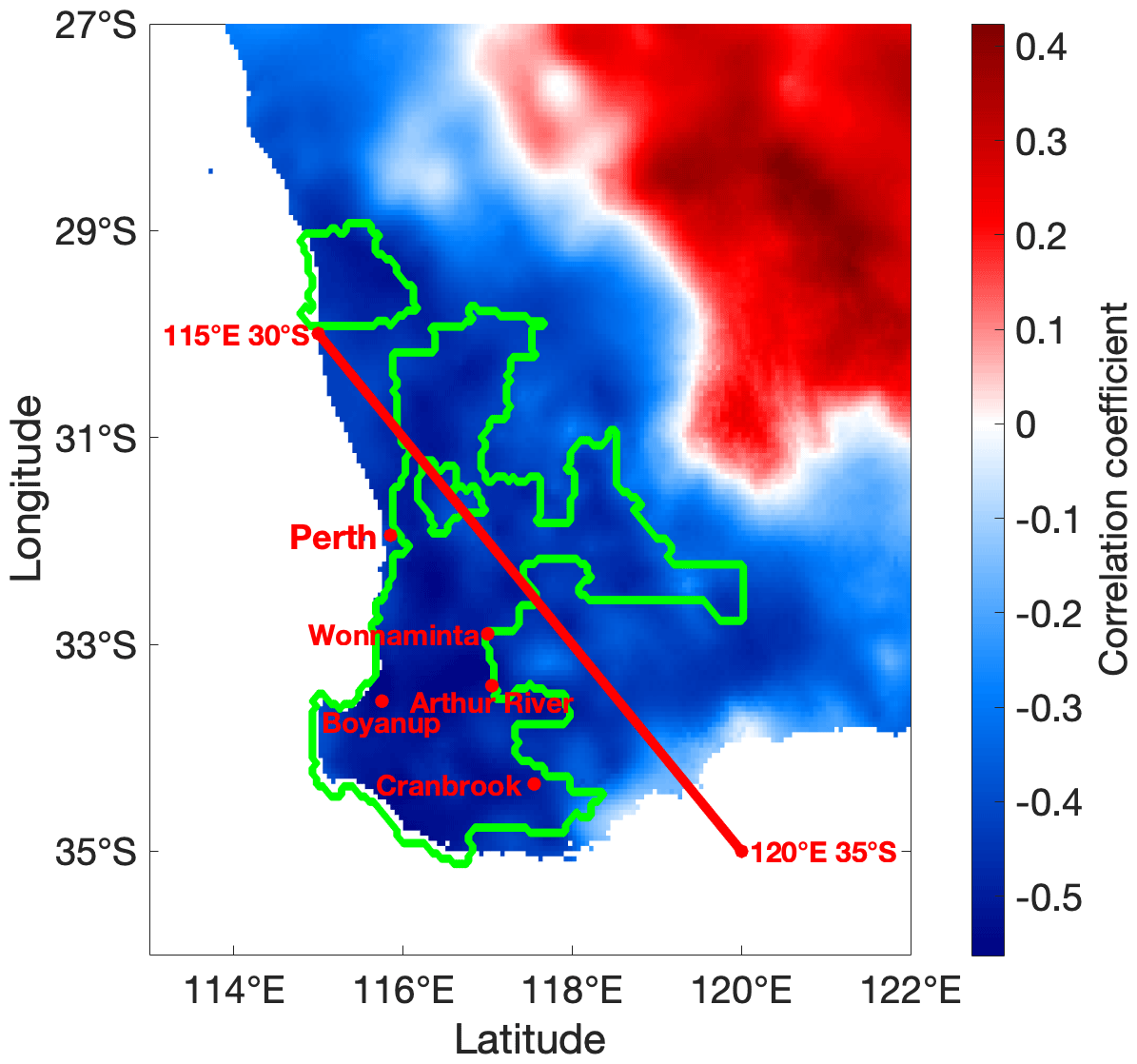
Figure 1The correlation map for the southwestern part of the WA region for a 6-year window for AWAP rainfall and DSS snow accumulation from 1900 to 2015 CE. The outlined area (green line) is the MASK region where the correlation is statistically significant (p < 0.05). The red diagonal line connecting 30∘ S, 115∘ E and 35∘ S, 120∘ E is the boundary of SWWA (van Ommen and Morgan, 2010). Perth is the capital city of WA. Boyanup, Wonnaminta, Arthur River and Cranbrook are the four significant (6-year window, p < 0.05) stations.
The correlation map (Fig. 1) shows the correlation coefficients for 6-year smoothed AWAP rainfall and DSS snow accumulation. The map shows that the strongly negatively correlated (r ≤ −0.5) areas are mainly concentrated in the southwestern corner. Areas in the top right show positive correlations with no statistical significance (p > 0.05). MASK covers almost the whole SWWA region apart from some coastal areas in the south. Southern coastal areas show no statistical significance (p > 0.05), which is consistent with the findings of van Ommen and Morgan (2010) who reported local rainfall on the south coast related to onshore northward flow that weakens the anticorrelation with DSS that prevails across the rest of the region.
In order to quantify the MASK correlation coefficient and evaluate the statistical significance, we multiply the MASK matrix (areas inside the region have a value of one, and areas outside of the region have a value of zero) of the MASK by the AWAP gridded data to generate the MASK rainfall. Hereafter, the SWWA rainfall that we describe is the MASK rainfall for the MASK region, as delineated in Fig. 1. We then calculate the SWWA rainfall correlation coefficient with DSS and test its statistical significance.
Table 3The Pearson correlation coefficients for SWWA rainfall and the four BoM stations' rainfall with the DSS snow accumulation. R2 is the square of the correlation coefficient. All of the correlations are statistically significant (6-year window, p < 0.05).
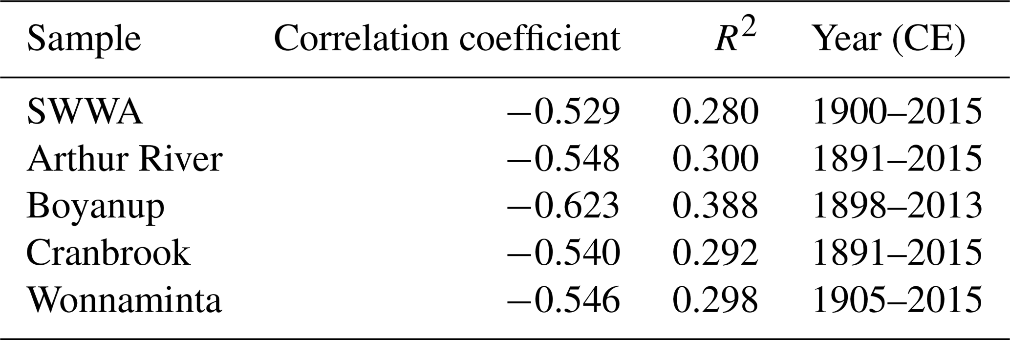
Table 3 integrates the results of the significance testing and correlations. The SWWA rainfall and DSS snow accumulation show a strong negative significant correlation (p < 0.05). The BoM stations' rainfall data also show consistent results. From the 15 stations tested, there are statistically significant (p < 0.05) correlations with DSS for 4 stations. These four stations are all geographically located in the MASK region (Fig. 1), showing the consistent significance of MASK. Five other stations within the region have correlations of a similar magnitude, but these correlations are not significant at the 5 % probability level (Fig. S4 in the Supplement). The squares of the correlation coefficients show that the explained variance is around 30 %–40 %. We note that the tropics and subtropics can also play an important role in driving rainfall changes in SWWA (Smith et al., 2000; England et al., 2006; Ummenhofer et al., 2008). Nevertheless, using Law Dome accumulation to reconstruct SWWA rainfall focuses on the SAM-related component of the rain-bearing systems, not the tropical or subtropical components. However, our analysis shows that it makes a valuable contribution to our ability to reconstruct past climate and so we construct a linear model for SWWA rainfall and DSS snow accumulation.
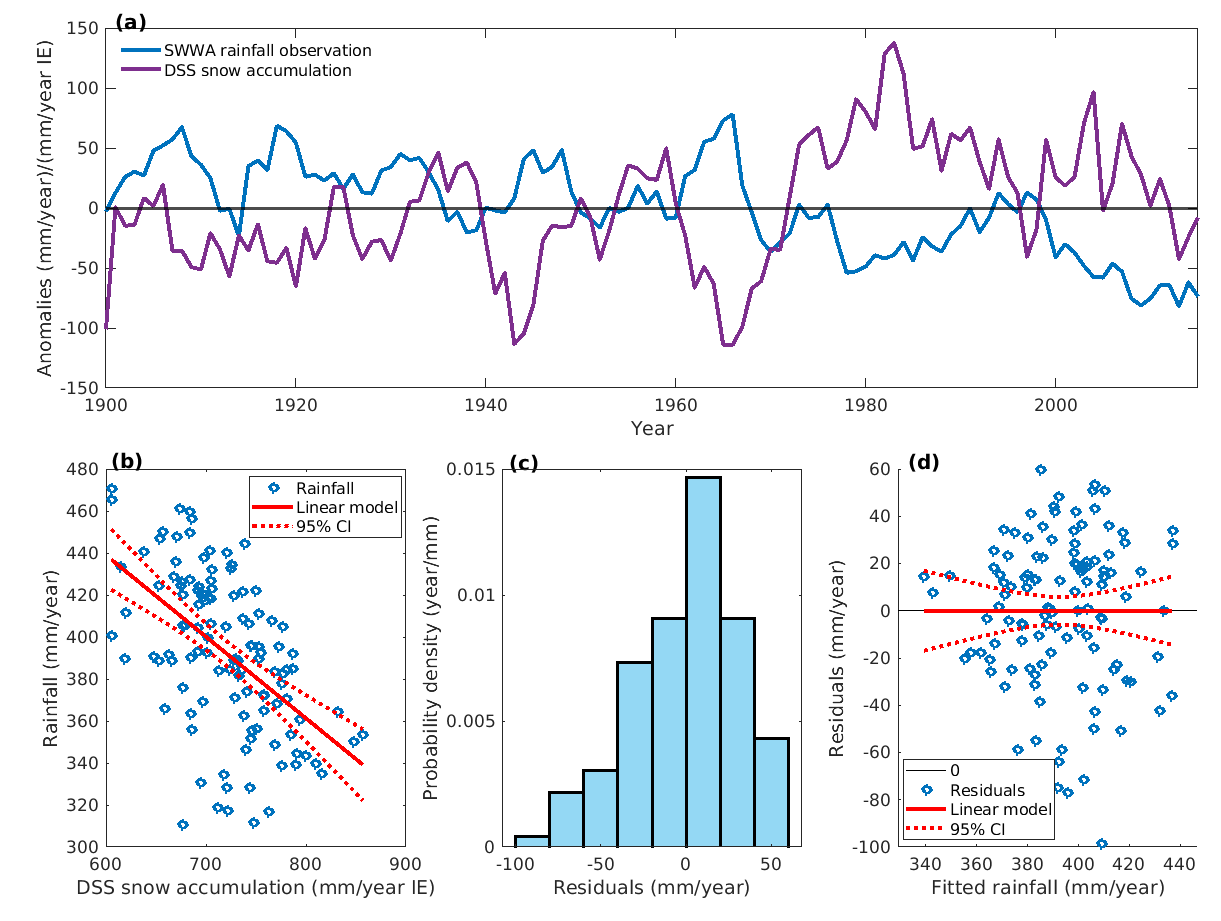
Figure 2(a) Time series of anomalies for AWAP rainfall in the MASK region and time series of DSS snow accumulation (6-year running averages) for the period from 1900 to 2015 CE. (b) Scatter plot of AWAP rainfall in the MASK region and DSS snow accumulation (6-year running averages) for the period from 1900 to 2015 CE with their linear models and 95 % confidence intervals. (c) The probability density function histogram for the model residuals. (d) Scatter plot for model residuals and fitted data with their linear fits and 95 % confidence intervals.
3.3 Linear model construction
The time series and the scatter plot for SWWA rainfall and DSS snow accumulation are shown in Fig. 2a and b respectively. The data show a generally linear distribution with a negative slope (Fig. 2b). We use ordinary least squares linear regression to construct a linear model for SWWA rainfall and DSS snow accumulation (for the four BoM stations, see Fig. S3 in the Supplement), and we estimate the 95 % confidence interval (CI) in the gradient and the intercept as 1.96 multiplied by the standard error of the model.
The model is rain = snow ⋅ (−0.389 ± 0.114) + 672 ± 82 mm yr−1 in the growing season for the period from 1900 to 2015 CE. The gradient interval [−0.503, −0.274] is always negative, which is consistent with the result from the Pearson correlation test: the coefficient is negative and statistically significant (p < 0.05).
Figure 2c is a histogram of the raw residuals using probability density function scaling. Residuals broadly follow a normal distribution. Figure 2d is a scatter plot of fitted rainfall data and residuals. The distribution of residuals has no obvious regularity or trend and is generally symmetric along y=0. Furthermore, we assess the robustness of the model in Sect. S5 in the Supplement. We calculate the autocorrelation length (where the autocorrelation coefficient is equal to or below zero) of the SWWA rainfall for the period from 1900 to 2015 CE and perform a jackknife (modified) analysis. The correlation coefficients of each individual jackknife ensemble member are all consistent with the period from 1900 to 2015 CE (Table S4 in the Supplement), and the 95 % confidence intervals for the gradient and intercept overlap (Table S4), showing the statistical indistinguishability between each individual jackknife ensemble member. Taken together, there is no obvious evidence to reject the linear model. Thus, we use this linear model and the time series of DSS snow accumulation to reconstruct SWWA rainfall from 2015 CE back to 22 BCE.
3.4 CUSUM analysis
The cumulative summation (CUSUM) technique has been used to investigate rainfall data (Kampata et al., 2008; Chowdhury and Beecham, 2010). CUSUM is a method to sum the data anomalies using
where x′ is the anomaly relative to the mean of the whole series (Chowdhury and Beecham, 2010). The aim of CUSUM is to identify the step change in a time series by continuously accumulating anomalies. A step in the original data would be identified by the change in the gradient of the CUSUM data.
Numerical integration enhances the signal-to-noise ratio. Using the CUSUM data to both pick the break point (and evaluate its significance) and estimate the timing uncertainty potentially offers advantages compared with using the original data, especially at lower signal-to-noise ratios.
To specifically determine the break point and evaluate its significance, we use the BREAKFIT analysis software (Mudelsee, 2009) on the CUSUM data.
3.5 Interpolation and data–model comparison
In light of the different spatial resolutions of the model simulations and AWAP gridded rainfall, we perform an interpolation so that model simulations are the same geospatial resolution as the AWAP gridded rainfall; we then multiply the MASK matrix by the interpolated model simulations to consistently capture the same region.
The rainfall reconstruction of SWWA back to 22 BCE is carried out using the linear model over MASK region, where the AWAP gridded rainfall and the DSS snow accumulation data are statistically significantly correlated. The rainfall simulation is the precipitation simulation of the CSIRO Mk3L model, run as four ensembles combining four climate forcings (Table 2). We use the CUSUM analysis to compare the simulation of each ensemble and three members of CONTROL (a pre-industrial control simulation; Phipps et al., 2013a) to the rainfall reconstruction. Also, as each ensemble member represents the different randomly initialised weather states, we compare the mean of each ensemble member to the rainfall reconstruction to estimate the uncertainties in the simulated rainfall.
To statistically compare the rainfall reconstruction with the model simulations and test the differences, we use Welch's t test to calculate the adapted t statistics using
where and , and , and n1 and n2 are sample mean values, standard deviations and sample sizes for two samples respectively. We also estimate the adapted degrees of freedom (DFs) using the Welch–Satterthwaite equation:
Taken together, we calculate the p value using t statistics and DFs.
To evaluate the specific time period that we are interested in, for example, the rainfall before and after 1850 CE, we calculate the root-mean-square error (RMSE) between reconstructions and model simulations, and also calculate the Pearson correlation coefficients, ESS (Eq. 1), and the Student's t statistic (Eq. 2) and its adjusted p value.

Figure 3(a) The rainfall reconstruction in the significant region in SWWA (the MASK region; Fig. 1) from 22 BCE to 2015 CE. The mean of this 2038-year time series (405 mm yr−1) is shown as a black horizontal line. (b) The CUSUM rainfall reconstruction (Eq. 3). The black horizontal line represents zero. The red vertical dashed lines highlight the years 1850 and 1971 CE. (c) The 45-year running change in the CUSUM rainfall reconstruction series. The red horizontal dashed line represents −1000 mm (accumulated change).
4.1 Rainfall reconstruction
Figure 3a shows the reconstructed SWWA rainfall time series for the growing season (May to October) from 22 BCE to 2015 CE. We further validate the rainfall reconstruction in Sect. S5 in the Supplement. We have found that the temporal stability of large-scale circulation over the mid-latitude Australasian and higher-latitude Law Dome regions is consistent, which is indicated by the correlation fields between Law Dome precipitation and mean sea level pressure in each member of the CSIRO Mk3L OGSV ensemble (Fig. S5 in the Supplement). This rainfall reconstruction has shown that it is possible to use ice cores to investigate the longer-term context of rainfall variability over SWWA prior to the instrumental era. We should also be aware that the Law Dome–SWWA precipitation correlation is stronger during periods of enhanced (stronger/more frequent) meridional circulation, whereas it is weaker during periods of weaker meridional circulation (van Ommen and Morgan, 2010). Thus, the robustness of the reconstruction may be reduced during periods of reduced meridional flow between southern Australia and Law Dome (Sect. S5 in the Supplement). Furthermore, the CSIRO Mk3L simulations exhibit variability in the correlation between Law Dome accumulation and SWWA precipitation on decadal to centennial timescales (Fig. S6 in the Supplement). Therefore, some caution is needed when interpreting the reconstruction. We choose 1850 CE to be the year that separates before and after the Industrial Revolution, consistent with other studies (e.g. Stocker et al., 2013).
Next, we assess whether the growing season rainfall in SWWA before and after 1850 CE belongs to the same distribution. We divide the rainfall reconstruction into two periods: 22 BCE to 1849 CE and 1851 to 2015 CE. We plot the empirical distribution function (Fig. 4a) and probability density function scaling histogram (Fig. 4b) for each sample as well as its corresponding normal distribution (black dashed line) with the same mean and standard deviation.
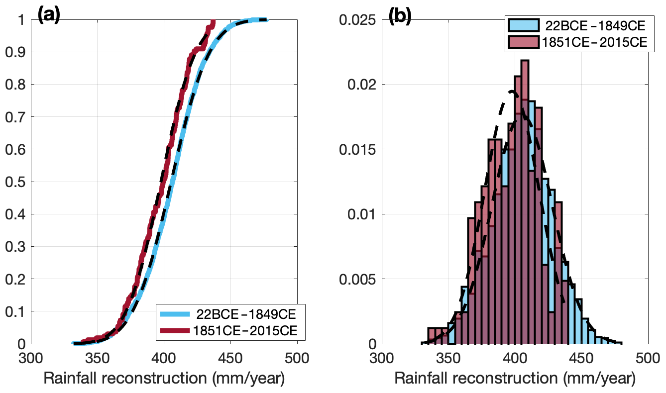
Figure 4(a) Empirical distribution function plot for rainfall reconstruction samples from 22 BCE to 1849 CE (blue curve) and from 1851 to 2015 CE (red curve). (b) Probability density function scaling histogram for two samples. The black dashed curves are each sample's corresponding normal distribution.
The distribution functions (Fig. 4) for the period from 1851 to 2015 CE are shifted left relative to the period from 22 BCE to 1849 CE, indicating that rainfall has decreased after 1850 CE. To quantify the rainfall reduction and test its statistical significance, we perform a two-sample KS test on the two samples and independently conduct a Welch's t test to validate the two-sample KS non-parametric test results.
Results from the two-sample KS test reject (p < 0.01) the null hypothesis that the samples are from same continuous distribution. Independently, the Welch's t test also allows us to reject (p < 0.01) the null hypothesis that the means are equal.
The mean of the growing season rainfall reconstruction for 1851 to 2015 CE is 398 mm yr−1, which is around 98 % of the rainfall mean from 22 BCE to 1849 CE (405 mm yr−1). The attenuation of the rainfall before and after 1850 CE is statistically significant, but the degree is around 2 %. The 1851–2015 CE sample is missing the higher end of the distribution (i.e. there are no years with rainfall greater than 440 mm yr−1), and this lack of recharging events might have more of an impact than the shift in the mean (e.g. Gallant et al., 2013). Moreover, the 1851–2015 CE sample has a lower low end of the distribution than the 22 BCE–1849 CE sample, indicating more prevalent dry years. This suggests the possibility of an anthropogenic influence on the hydroclimate of this region.
The time series of the rainfall reconstruction indicates that another rainfall attenuation event may have occurred after 1850 CE, around the late 20th century (Fig. 3a, b). In order to accurately determine the changes in rainfall after 1850 CE, we calculate the CUSUM time series (Eq. 3) for the rainfall time series (Fig. 3a) and use BREAKFIT analysis to identify any significant changes in the gradient. As CUSUM continuously accumulates anomalies in the rainfall reconstruction along the timeline, the variability in the rainfall becomes clearly visually observable (Fig. 3b). The sign and magnitude of the gradient of the CUSUM plot indicate rainfall anomalies: a positive (negative) gradient indicates a positive (negative) anomaly corresponding to a rainfall increase (decrease) event. The larger the magnitude, the higher the degree of the event. For consistency with the duration of the simulated rainfall, which is available from 501 to 2000 CE, we take the rainfall reconstruction for the same period to calculate the CUSUM time series and conduct BREAKFIT analysis.
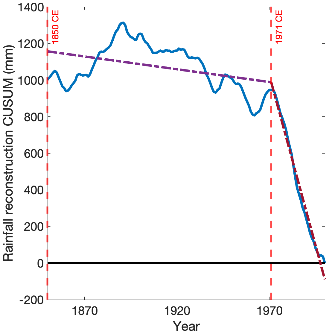
Figure 5CUSUM time series on rainfall reconstruction for the period from 1850 to 2000 CE. The yellow dotted lines are each interval's gradient calculated using BREAKFIT analysis, with 1971 CE identified as the break point. The gradient before 1971 CE is −1.40 mm yr−1; the gradient after 1971 CE is −37.16 mm yr−1.
Figure 5 shows the rainfall reconstruction CUSUM time series from 1850 to 2000 CE. Results from BREAKFIT show that the break point is at 1971 CE ± 7 years (95 % CI). The gradients for the intervals [1850, 1971] CE and [1971, 2000] CE are −1.4 mm yr−1 [−3.2, −0.4] and −37.16 mm yr−1 [−45.9, −28.8] respectively. Thus, the break in the gradient at 1971 is statistically significant.
We test the findings of break-point analysis on the CUSUM time series by analysis of the original data. Breaking the rainfall into two samples, we found a shift of the distribution to lower rainfall after 1971 CE in both the empirical distribution function (Fig. 6a) and the probability density function scaling histogram (Fig. 6b). The shift is around 30 mm yr−1, showing a nearly 8 % attenuation after 1971 CE, more than 4 times the reduction from 1850 CE. Two further statistical tests were preformed to verify this finding.
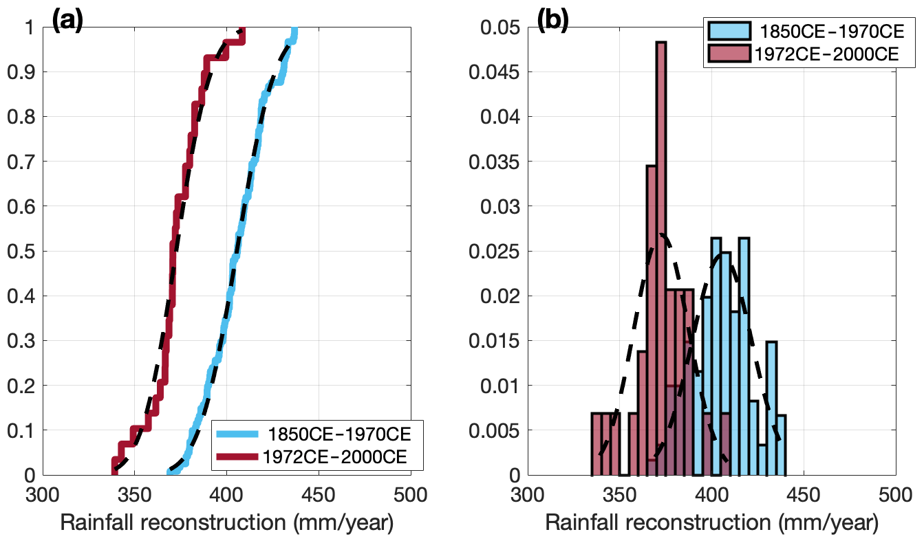
Figure 6(a) Empirical distribution function plot for rainfall reconstruction samples from 1850 to 1970 CE (blue curve) and from 1972 to 2000 CE (red curve). (b) Probability density function scaling histogram for two samples. The black dashed curves are each sample's corresponding normal distribution.
Results from the two-sample KS test allow us to reject the null hypothesis (p < 0.01) that the samples are from the same continuous distribution. Independently, it is statistically significant (p < 0.01) that the result from the Welch's t test can also allow us to reject the null hypothesis that the two samples have equal means. The mean rainfall during the period from 1972 to 2000 CE is 373 mm yr−1, which is 92 % of the mean rainfall during the period from 1850 to 1970 CE (406 mm yr−1). This change is more than 4 times bigger than the change around 1850 CE. Not only is there a large reduction in the mean rainfall, but the 1972 to 2000 CE sample's distribution has also largely shifted to lower values compared with 1850 to 1970 CE. There are no years with rainfall over 410 mm yr−1, and nearly half of the years have rainfall of less than 375 mm yr−1 in the 1972 to 2000 CE sample (Fig. 6b). This likely has a larger impact on agriculture than the rainfall shift before and after 1850 CE.
Results from the two individual statistical tests are very consistent with the BREAKFIT analysis results on the CUSUM time series which indicate that 1971 CE marks the change in gradients from 1850 to 2000 CE. Comparison of Fig. 6 with Fig. 4 reveals that the shift in the rainfall distribution at around 1971 CE was much more pronounced than the shift at around 1850 CE. The reduction in the mean rainfall at around 1971 CE resulted in a prolonged drought in SWWA. This drought continued during the 2015–2020 CE period (Fig. S7 in the Supplement). To highlight dry epochs of an equivalent duration to the observed drought to date, we calculate the 45-year running change in the CUSUM time series (Fig. 3c). Over the 45 years from 1971 to 2015 CE, this prolonged drought is expressed by an integrated rainfall reduction of more than 1000 mm (Fig. 3c). We note there are two comparable prior epochs during the past two millennia: from around 385 to 429 CE and from around 732 to 776 CE (Fig. 3c).
4.2 Data–model comparison
Consistent with the analysis applied to the rainfall reconstruction, we analyse the simulated rainfall from CONTROL and the four forced ensembles. We divide the simulated time series for each simulation into two samples: 501–1849 CE and 1851–2000 CE. We further divide the industrial period into samples before and after the observed shift in 1971 CE. We then independently perform the two-sample KS test and the Welch's t test. We also use two different metrics to assess the degree of agreement between the CUSUM time series for the various model simulations and the reconstruction: the differences in the slope and the root-mean-square error (RMSE).
Summary statistics for the model simulations are shown in Table S5 in the Supplement. The model can be seen to have a dry bias, but the simulated internal variability is of a similar magnitude (∼ 80 %) to the reconstruction. The simulated rainfall for each individual ensemble member is shown in Fig. S8 in the Supplement, with the corresponding CUSUM time series shown in Fig. S9 in the Supplement. Within each forced ensemble, there are considerable differences between the CUSUM time series for individual ensemble members. This highlights the role of unforced internal variability in driving SWWA rainfall, consistent with the findings of Cai and Shi (2005).
A number of prolonged droughts that approach the magnitude of the current integrated rainfall deficit are apparent in the reconstruction (Fig. 3c), as discussed in Sect. 4.1. These prior drought epochs occurred during the pre-industrial era, suggesting that they may have arisen through natural climate variability or natural forcings such as volcanoes. To explore this within the model simulations, the 45-year changes in the CUSUM time series for the pre-industrial control simulation are shown in Fig. S10 in the Supplement. A number of prolonged droughts are also apparent in all three ensemble members, for example, from 589 to 633 CE in Control1 (Fig. S10b). This supports the hypothesis that prolonged droughts of a similar magnitude to the currently observed drought can arise through natural climate variability or natural forcings.
4.2.1 Industrial era
We now examine the model ensembles and assess whether the simulated rainfall during the industrial era has a different distribution from the simulated rainfall during the pre-industrial era. We cannot reject the null hypothesis (with the two-sample KS test or Welch's t test performed on both the CONTROL and O series) that the rainfall in the 501–1849 CE and 1851–2000 CE periods is from the same distribution (KS test) or equal means (Welch's t test) (Table 4). Conversely, the results from both the two-sample KS test and the Welch's t test allow us to reject (p < 0.05) the null hypothesis for OG, OGS, OGSV and the rainfall reconstruction (Table 4). These results give us the confidence to say that orbital forcing is not the main driver of the rainfall changes after 1850 CE. Once the greenhouse gases are added to the model climate forcings, the rainfall simulations before and after 1850 CE belong to different distributions with different means (Table 4). There is no change when the solar irradiance and volcanic aerosols are added. Based on these statistical tests, we suggest that there is evidence that anthropogenic greenhouse gases play a role; however, there is no evidence of any additional impacts due to either solar irradiance or volcanic aerosols.
Table 4The results for two independent statistical tests for different time periods from the rainfall time series. “KS test” is the two-sample KS test, and “W t test” is the Welch's t test. “Same” means that we cannot reject the null hypothesis (the two samples of data are from the same distribution), whereas “Different” means that we can reject the null hypothesis (p < 0.05).
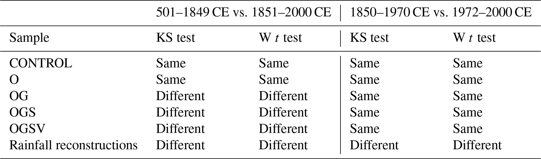

Figure 7CUSUM time series for the rainfall reconstruction and CSIRO Mk3L model rainfall simulations in the MASK region from 501 to 2000 CE. The model simulations include CONTROL (pre-industrial control simulation; Phipps et al., 2013a), O, OG, OGS and OGSV. The black horizontal line represents zero. The red vertical dashed lines highlight the years 1850 and 1971 CE.
Figure 7 shows the CUSUM time series for each of the rainfall reconstruction and CSIRO Mk3L model simulations from 501 to 2000 CE. For each ensemble including the CONTROL scenario, the CUSUM time series is calculated using the mean of the three ensemble members. As for the statistical tests (Table 4), the CUSUM time series in Fig. 7 show that the rainfall change around 1850 CE is not simulated by the CONTROL or O ensembles, but it is simulated by the OG, OGS and OGSV ensemble series.
Examining each of the respective ensembles, we see that CONTROL does not capture the key features of the rainfall reconstruction (Fig. 7). This suggests either a role of internal variability or that climate forcings might be driving the rainfall changes in SWWA. The time series of O varies slightly around zero with no obvious gradient changes (Fig. 7), which suggests that orbital forcing alone cannot explain the changes in SWWA rainfall in recent decades. In contrast, ensembles OG, OGS and OGSV are able to reproduce some of the key features of the rainfall reconstruction, particularly the decline after 1850 CE. These ensembles have approximately equal magnitudes, especially after around 1900 CE, and their gradient changes are broadly synchronous with large negative magnitudes.
4.2.2 Late 20th century
Figure 8 shows the CUSUM time series for the rainfall reconstruction and simulations for 1972–2000 CE. Ensemble O shows that the orbital forcing cannot explain the rainfall reduction after 1971 CE; however, the reduction is reproduced by ensembles OG, OGS and OGSV. All three ensembles have the same sign of gradients and similar magnitudes. The magnitude of the gradient for the rainfall reconstruction is larger than any of the rainfall simulations.
We also perform a two-sample KS test and a Welch's t test on the rainfall simulations for the 1850–1970 CE and 1972–2000 CE periods. None of the model results from the statistical tests allow us to reject the null hypothesis with statistical significance. Unlike the rainfall reconstruction, none of the model simulations show that the rainfall in the 1972–2000 CE period is different from the 1850–1970 CE period (Table 4).

Figure 8The CUSUM time series for the rainfall reconstruction and simulations for the period from 1972 to 2000 CE from the 501–2000 CE series. The black horizontal line represents zero.
Table 5The RMSE and difference in slope calculated between the rainfall reconstruction and simulations in the period from 1972 to 2000 CE. The difference in slope is the difference of the slope of the ordinary least squares linear fitted CUSUM time series data for each sample to the slope of the fitted CUSUM time series data for rainfall reconstruction in the period from 1972 to 2000 CE.
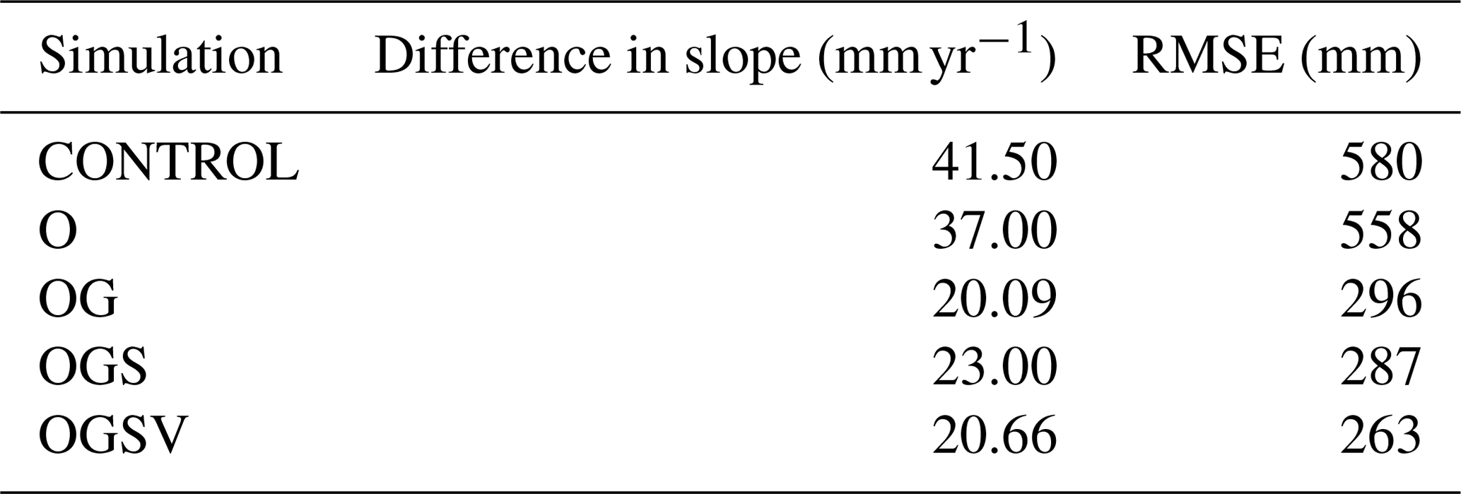
As we can see in Fig. 8, CONTROL and O have a negligible slope; however, OG, OGS and OGSV exhibit a negative slope and are, therefore, much closer to the rainfall reconstruction. We note that the amplitude of the internal variability in the underlying raw time series will influence the magnitude of the slopes in the CUSUM analysis. CONTROL and O are essentially indistinguishable, as the time frame of orbital forcing is long compared with the 30-year period studied here. To determine which model simulation is in best agreement with the rainfall reconstruction, we calculate the difference in slope and the root-mean-square error (RMSE) (Table 5) between the CUSUM time series for the rainfall reconstruction and each model ensemble.
Comparing CONTROL and the four ensembles, CONTROL and O have the largest differences in slope and RMSE, relative to the rainfall reconstruction, than any of the others. The forced ensembles, OG, OGS and OGSV, have much smaller differences in slope and a much smaller RMSE. Therefore, both the difference in slope and the RMSE analysis suggest that the simulations including greenhouse gases are the closest to the rainfall reconstruction. Including solar irradiance and volcanic aerosols has negligible additional impact.
Although the model ensembles that include greenhouse gas forcing do simulate a drying trend after 1971 CE, the simulated trend is weaker than in the reconstruction. This may reflect the influence of stratospheric ozone depletion, which is not modelled in the climate model simulations that we analyse in this study. Alternatively, it may reflect the role of natural climate variability. Because of its stochastic nature, the model simulations would not be expected to replicate the phase or magnitude of the specific internal variability encountered in the real world.
The largest improvement in agreement comes from adding greenhouse gases into the model. Therefore, our analysis suggests that greenhouse gases are the dominant climate forcing, out of the four natural and anthropogenic forcings considered in this study, driving the rainfall changes in SWWA during the 20th century.
We have used the DSS snow accumulation record to extend the previous published reconstruction of the SWWA growing season (May to October) rainfall. Based on the statistically significant (p < 0.05) negative correlation between SWWA rainfall and DSS snow accumulation in the growing season, we built a linear model and reconstructed the rainfall for 2038 years (22–2015 CE). Consistent with other studies (e.g. Stocker et al., 2013), we use 1850 CE to divide the reconstruction into two periods: before and after the industrial revolution. We independently performed a two-sample KS test and a Welch's t test to determine whether the two samples are from equal means and distributions. The results of the tests rejected (p < 0.01) the null hypotheses, suggesting a detectable change in SWWA rainfall much earlier than the observed climate shift in the region in the 1970s. The CUSUM time series and the BREAKFIT analysis suggest a rainfall reduction after 1971 CE that was much larger in magnitude than the reduction after 1850 CE. The rainfall means and distributions in the 1850–1970 CE and 1972–2000 CE periods are independently tested and are shown to be significantly (p < 0.01) different.
With statistically significant (p < 0.01) rainfall reductions after 1850 and after 1971 CE, we compared the rainfall reconstructions with ensembles of CSIRO Mk3L climate model simulations driven by different natural and anthropogenic climate forcings. Comparing the 501–1849 CE and 1851–2000 CE periods, the addition of greenhouse gases significantly (p < 0.05) changed the rainfall means and distributions for the two periods. There is no detectable influence from solar irradiance and volcanic aerosols. However, the rainfall means and distributions for the 1850–1970 CE and 1972–2000 CE periods are statistically indistinguishable.
Examining the CUSUM time series for the 1972–2000 CE period, we do not find any drying trend in the CONTROL simulation nor in simulations driven only with orbital forcing. However, we do find a drying trend in simulations that include anthropogenic greenhouse gases. We again find that solar irradiance and volcanic aerosols have negligible additional impact. Thus, the model simulations suggest that anthropogenic forcing has been the dominant driver of the rainfall trend in SWWA since 1971 CE.
Both the reconstruction and the climate model simulations suggest that the drying trend began earlier than the 1970s. However, the model simulations do not capture the acceleration in the reconstructed drying trend at around 1971 CE. This suggests that this acceleration cannot be attributed to external forcings – at least not any of the forcings considered in this study. Natural variability or stratospheric ozone depletion are potential alternative explanations (e.g. Cai and Shi, 2005). An investigation into possible ozone forcing and a comparison with multiple climate models is a promising avenue for future work.
The reconstruction reveals that the rainfall decrease in SWWA in recent decades is not unprecedented. We note that two previous prolonged drought events of similar magnitude in SWWA have occurred during the past 2 millennia. Droughts of similar duration and magnitude also occur in an unforced pre-industrial control simulation. Therefore, the model simulations support the hypothesis that these pre-industrial drought events may have arisen through natural climate variability. However, forced climate model simulations indicate that anthropogenic greenhouse gases are the dominant driver of the rainfall reduction in SWWA since the early 1970s.
The SWWA rainfall reconstruction data are available from https://doi.org/10.25959/5f4c50b7b661f (Zheng et al., 2020). The DSS snow accumulation record (Roberts et al., 2015) is available via https://doi.org/10.4225/15/57468B15E1E2B (Moy, 2016). The CSIRO Mk3L climate model simulations are available from https://doi.org/10.5281/zenodo.3908926 (Phipps et al., 2013b). The BoM instrumental rainfall records are available from http://www.bom.gov.au/climate/data/ (last access: 30 September 2021, Lavery et al., 1997). The AWAP AGCD data are available from http://www.bom.gov.au/metadata/catalogue/19115/ANZCW0503900567?template=full (last access: 30 September 2021, Jones et al., 2009).
The supplement related to this article is available online at: https://doi.org/10.5194/cp-17-1973-2021-supplement.
YZ, SJP, LMJ and JLR conceived the study. YZ performed the analysis. All authors contributed to writing the paper.
The authors declare that they have no conflict of interest.
Publisher's note: Copernicus Publications remains neutral with regard to jurisdictional claims in published maps and institutional affiliations.
This work was supported by the Centre for Southern Hemisphere Oceans Research, a joint research centre between the Qingdao National Laboratory for Marine Science and Technology (China) and the Commonwealth Scientific and Industrial Research Organisation (CSIRO; Australia).
This research has been supported by the Australian Government Department of Industry, Science, Energy and Resources (grant no. ASCI000002); the Australian Research Council (grant no. SR140300001); and the Australian Government Department of Agriculture, Water and the Environment (Australian Antarctic Science Project 4061, Australian Antarctic Science Project 4062 and Australian Antarctic Science Project 4537).
This paper was edited by Eric Wolff and reviewed by Matthew H. England and one anonymous referee.
Abram, N. J., Mulvaney, R., Vimeux, F., Phipps, S. J., Turner, J., and England, M. H.: Evolution of the Southern Annular Mode during the past millennium, Nat. Clim. Change, 4, 564–569, https://doi.org/10.1038/NCLIMATE2235, 2014. a
Anderson, W., Heinrich, A., and Abbotts, R.: Long-season Aust. J. Exp. Agr., 36, 203–208, 1996. a, b
Ansell, T., Reason, C., Smith, I., and Keay, K.: Evidence for decadal variability in southern Australian rainfall and relationships with regional pressure and sea surface temperature, Int. J. Climatol., 20, 1113–1129, 2000. a
Ashok, K., Guan, Z., and Yamagata, T.: Influence of the Indian Ocean Dipole on the Australian winter rainfall, Geophys. Res. Lett., 30, 1821, https://doi.org/10.1029/2003GL017926, 2003. a
Australian Government: Local Government Area [data set], available at: https://data.gov.au/data/dataset/8a8e0037-e474-422f-8026-241c7c88551f (last access: 30 September 2021), 2020. a, b
Barr, C., Tibby, J., Leng, M. J., Tyler, J. J., Henderson, A. C. G., Overpeck, J. T., Simpson, G. L., Cole, J. E., Phipps, S. J., Marshall, J. C., McGregor, G. B., Hua, Q., and McRobie, F. H.: Holocene El Niño-Southern Oscillation variability reflected in subtropical Australian precipitation, Sci. Rep.-UK, 9, 1627, https://doi.org/10.1038/s41598-019-38626-3, 2019. a
Bretherton, C. S., Widmann, M., Dymnikov, V. P., Wallace, J. M., and Bladé, I.: The effective number of spatial degrees of freedom of a time-varying field, J. Climate, 12, 1990–2009, 1999. a, b
Bromwich, D. H.: Snowfall in high southern latitudes, Rev. Geophys., 26, 149–168, 1988. a
Cai, W. and Cowan, T.: SAM and regional rainfall in IPCC AR4 models: Can anthropogenic forcing account for southwest Western Australian winter rainfall reduction?, Geophys. Res. Lett., 33, L24708, https://doi.org/10.1029/2006GL028037, 2006. a, b, c, d
Cai, W. and Shi, G.: Multidecadal fluctuations of winter rainfall over southwest Western Australia simulated in the CSIRO Mark 3 coupled model, Geophys. Res. Lett., 32, L12701, https://doi.org/10.1029/2005GL022712, 2005. a, b, c, d, e, f
Cai, W., Collier, M. A., Gordon, H. B., and Waterman, L. J.: Strong ENSO Variability and a Super-ENSO Pair in the CSIRO Mark 3 Coupled Climate Model, Mon. Weather Rev., 131, 1189–1210, https://doi.org/10.1175/1520-0493(2003)131<1189:SEVAAS>2.0.CO;2, 2003. a, b
Cai, W., Van Rensch, P., Cowan, T., and Hendon, H. H.: Teleconnection pathways of ENSO and the IOD and the mechanisms for impacts on Australian rainfall, J. Climate, 24, 3910–3923, 2011. a
Chiew, F. H., Piechota, T. C., Dracup, J. A., and McMahon, T. A.: El Nino/Southern Oscillation and Australian rainfall, streamflow and drought: Links and potential for forecasting, J. Hydrol., 204, 138–149, 1998. a
Chowdhury, R. and Beecham, S.: Australian rainfall trends and their relation to the southern oscillation index, Hydrol. Process., 24, 504–514, 2010. a, b
England, M. H., Ummenhofer, C. C., and Santoso, A.: Interannual rainfall extremes over southwest Western Australia linked to Indian Ocean climate variability, J. Climate, 19, 1948–1969, 2006. a, b, c, d, e
Feng, J., Li, J., and Li, Y.: A monsoon-like southwest Australian circulation and its relation with rainfall in southwest Western Australia, J. Climate, 23, 1334–1353, 2010. a
Fierro, A. O. and Leslie, L. M.: Links between central west Western Australian rainfall variability and large-scale climate drivers, J. Climate, 26, 2222–2246, 2013. a, b
French, R. and Schultz, J.: Water use efficiency of wheat in a Mediterranean-type environment. II. Some limitations to efficiency, Aust. J. Agr. Res., 35, 765–775, 1984. a
Gallant, A. J., Reeder, M. J., Risbey, J. S., and Hennessy, K. J.: The characteristics of seasonal-scale droughts in Australia, 1911–2009, Int. J. Climatol., 33, 1658–1672, 2013. a
Gillett, N. P. and Thompson, D. W. J.: Simulation of Recent Southern Hemisphere Climate Change, Science, 302, 273–275, https://doi.org/10.1126/science.1087440, 2003. a
Gong, D. and Wang, S.: Definition of Antarctic oscillation index, Geophys. Res. Lett., 26, 459–462, 1999. a
Goodwin, I., Van Ommen, T., Curran, M., and Mayewski, P.: Mid latitude winter climate variability in the South Indian and southwest Pacific regions since 1300 AD, Clim. Dynam., 22, 783–794, 2004. a
Gordon, H. B., Rotstayn, L. D., McGregor, J. L., Dix, M. R., Kowalczyk, E. A., O'Farrell, S. P., Waterman, L. J., Hirst, A. C., Wilson, S. G., Collier, M. A., Watterson, I. G., and Elliott, T. I.: The CSIRO Mk3 Climate System Model, Technical Paper 60, CSIRO Atmospheric Research, available at: http://www.cmar.csiro.au/e-print/open/gordon_2002a.pdf (last access: 30 September 2021), 2002. a
Hennessy, K. J., Suppiah, R., and Page, C. M.: Australian rainfall changes, 1910–1995, Aust. Meteorol. Mag., 48, 1–13, 1999. a
Hope, P. K., Drosdowsky, W., and Nicholls, N.: Shifts in the synoptic systems influencing southwest Western Australia, Clim. Dynam., 26, 751–764, 2006. a
Jones, D. A., Wang, W., and Fawcett, R.: High-quality spatial climate data-sets for Australia, Aust. Meteorol. Ocean. J., 58, 233–248, 2009 (data available at: https://doi.org/10.4227/166/5a8647d1c23e0, last access: 30 September 2021). a, b, c
Kampata, J. M., Parida, B. P., and Moalafhi, D.: Trend analysis of rainfall in the headstreams of the Zambezi River Basin in Zambia, Phys. Chem. Earth Pt. A/B/C, 33, 621–625, 2008. a
Lavery, B., Joung, G., and Nicholls, N.: An extended high-quality historical rainfall dataset for Australia, Aust. Meteorol. Mag., 46, 27–38, 1997 (data available at http://www.bom.gov.au/climate/data/, last access: 30 September 2021). a, b
Li, Y., Cai, W., and Campbell, E.: Statistical modeling of extreme rainfall in southwest Western Australia, J. Climate, 18, 852–863, 2005. a
Ludwig, F. and Asseng, S.: Climate change impacts on wheat production in a Mediterranean environment in Western Australia, Agr. Syst., 90, 159–179, 2006. a, b, c
Ludwig, F., Milroy, S. P., and Asseng, S.: Impacts of recent climate change on wheat production systems in Western Australia, Clim. Change, 92, 495–517, 2009. a
Moy, A.: A 2000-year annual record of snow accumulation rates for Law Dome, East Antarctica, in: Ver. 1, Australian Antarctic Data Centre [data set], https://doi.org/10.4225/15/57468B15E1E2B, 2016. a
Mudelsee, M.: Break function regression, Eur. Phys. J.-Spec. Top., 174, 49–63, 2009 (code available at: https://doi.org/10.1140/epjst/e2009-01089-3, last access: 30 September 2021). a
Phipps, S. J., Rotstayn, L. D., Gordon, H. B., Roberts, J. L., Hirst, A. C., and Budd, W. F.: The CSIRO Mk3L climate system model version 1.0 – Part 1: Description and evaluation, Geosci. Model Dev., 4, 483–509, https://doi.org/10.5194/gmd-4-483-2011, 2011. a, b, c, d
Phipps, S. J., Rotstayn, L. D., Gordon, H. B., Roberts, J. L., Hirst, A. C., and Budd, W. F.: The CSIRO Mk3L climate system model version 1.0 – Part 2: Response to external forcings, Geosci. Model Dev., 5, 649–682, https://doi.org/10.5194/gmd-5-649-2012, 2012. a, b
Phipps, S. J., McGregor, H. V., Gergis, J., Gallant, A. J., Neukom, R., Stevenson, S., Ackerley, D., Brown, J. R., Fischer, M. J., and van Ommen, T. D.: Paleoclimate data–model comparison and the role of climate forcings over the past 1500 years, J. Climate, 26, 6915–6936, 2013a. a, b, c, d, e, f
Phipps, S. J., McGregor, H. V., Gergis, J., Gallant, A. J. E., Neukom, R., Stevenson, S., Ackerley, D., Brown, J. R., Fischer, M. J., and van Ommen, T. D.: Paleoclimate Data-Model Comparison and the Role of Climate Forcings over the Past 1500 Years, in: Journal of Climate (Vol. 26, Number 18, pp. 6915–6936), Zenodo [data set], https://doi.org/10.5281/zenodo.3908927, 2013b. a
Pitman, A. J., Narisma, G. T., Pielke Sr, R. A., and Holbrook, N.: Impact of land cover change on the climate of southwest Western Australia, J. Geophys. Res.-Atmos., 109, D18109, https://doi.org/10.1029/2003JD004347, 2004. a, b, c, d, e
Pittock, A.: Recent climatic change in Australia: Implications for a CO2-warmed earth, Clim. Change, 5, 321–340, 1983. a, b
Power, S., Sadler, B., and Nicholls, N.: The influence of climate science on water management in Western Australia: Lessons for climate scientists, B. Am. Meteorol. Soc., 86, 839–844, 2005. a, b
Roberts, J., Plummer, C., Vance, T., van Ommen, T., Moy, A., Poynter, S., Treverrow, A., Curran, M., and George, S.: A 2000-year annual record of snow accumulation rates for Law Dome, East Antarctica, Clim. Past, 11, 697–707, https://doi.org/10.5194/cp-11-697-2015, 2015. a, b, c, d, e, f, g
Samuel, J. M., Verdon, D. C., Sivapalan, M., and Franks, S. W.: Influence of Indian Ocean sea surface temperature variability on southwest Western Australian winter rainfall, Water Resour. Res., 42, W08402, https://doi.org/10.1029/2005WR004672, 2006. a, b
Siddique, K., Loss, S., Regan, K., and Jettner, R.: Adaptation and seed yield of cool season grain legumes in Mediterranean environments of south-western Australia, Aust. J. Agr. Res., 50, 375–388, 1999. a
Smith, I., McIntosh, P., Ansell, T., Reason, C., and McInnes, K.: Southwest Western Australian winter rainfall and its association with Indian Ocean climate variability, Int. J. Climatol., 20, 1913–1930, 2000. a, b
Stocker, T. F., Qin, D., Plattner, G.-K., Tignor, M., Allen, S. K., Boschung, J., Nauels, A., Xia, Y., Bex, V., Midgley, P. M.: Climate change 2013: The physical science basis, Contribution of working group I to the fifth assessment report of the intergovernmental panel on climate change, 1535 pp., 2013. a, b
Thompson, D. W. and Solomon, S.: Interpretation of recent Southern Hemisphere climate change, Science, 296, 895–899, 2002. a
Thompson, D. W., Solomon, S., Kushner, P. J., England, M. H., Grise, K. M., and Karoly, D. J.: Signatures of the Antarctic ozone hole in Southern Hemisphere surface climate change, Nat. Geosci., 4, 741–749, 2011. a
Timbal, B., Arblaster, J. M., and Power, S.: Attribution of the late-twentieth-century rainfall decline in southwest Australia, J. Climate, 19, 2046–2062, 2006. a, b, c
Trenberth, K. E. and Hoar, T. J.: El Niño and climate change, Geophys. Res. Lett., 24, 3057–3060, 1997. a
Ummenhofer, C. C., Sen Gupta, A., Pook, M. J., and England, M. H.: Anomalous rainfall over southwest Western Australia forced by Indian Ocean sea surface temperatures, J. Climate, 21, 5113–5134, 2008. a, b
van Ommen, T. D. and Morgan, V.: Snowfall increase in coastal East Antarctica linked with southwest Western Australian drought, Nat. Geosci., 3, 267–272, 2010. a, b, c, d, e, f, g, h, i, j
Ward, P. and Dunin, F.: Growing season evapotranspiration from duplex soils in south-western Australia, Agr. Water Manage., 50, 141–159, 2001. a
Watson, E. and Lapins, P.: Losses of nitrogen from urine on soils from south western Australia, Aust. J. Exp. Agr., 9, 85–91, 1969. a
Wright, P. B.: Seasonal rainfall in southwestern Australia and the general circulation, Mon. Weather Rev., 102, 219–232, 1974a. a, b
Wright, P. B.: Temporal variations in seasonal rainfalls in southwestern Australia, Mon. Weather Rev., 102, 233–243, 1974b. a
Yu, B. and Neil, D.: Long-term variations in regional rainfall in the south-west of Western Australia and the difference between average and high intensity rainfalls, Int. J. Climatol., 13, 77–88, 1993. a
Zheng, Y., Phipps, S., Roberts, J., and Jong, L. M.: Extending and understanding the South West Western Australian rainfall record using the Dome Summit South ice core, East Antarctica, Institute for Marine and Antarctic Studies (IMAS), University of Tasmania (UTAS) [data set], https://doi.org/10.25959/5f4c50b7b661f, 2020. a