El Niño–Southern Oscillation and internal sea surface temperature variability in the tropical Indian Ocean since 1675

The dominant modes of climate variability on interannual timescales in the tropical Indian Ocean are the El Niño–Southern Oscillation (ENSO) and the Indian Ocean Dipole. El Niño events have occurred more frequently during recent decades, and it has been suggested that an asymmetric ENSO teleconnection (warming during El Niño events is stronger than cooling during La Niña events) caused the pronounced warming of the western Indian Ocean. In this study, we test this hypothesis using coral Sr∕Ca records from the central Indian Ocean (Chagos Archipelago) to reconstruct past sea surface temperatures (SSTs) in time windows from the mid-Little Ice Age (1675–1716) to the present. Three sub-fossil massive Porites corals were dated to the 17–18th century (one coral) and the 19–20th century (two corals). Their records were compared with a published modern coral Sr∕Ca record from the same site. All corals were subsampled at a monthly resolution for Sr∕Ca measurements, which were measured using a simultaneous inductively coupled plasma optical emission spectrometer (ICP-OES). Wavelet coherence analysis shows that interannual variability in the four coral records is driven by ENSO, suggesting that the ENSO–SST teleconnection in the central Indian Ocean has been stationary since the 17th century. To determine the symmetry of El Niño and La Niña events, we compiled composite records of positive and negative ENSO-driven SST anomaly events. We find similar magnitudes of warm and cold anomalies, indicating a symmetric ENSO response in the tropical Indian Ocean. This suggests that ENSO is not the main driver of central Indian Ocean warming.

1 Introduction

As the impacts of global climate change increase, paleoclimate research is more important than ever. The Indian Ocean is of major relevance to global ocean warming as it has been warming faster than any other ocean basin during the last century and is the largest contributor to the current rise of global mean sea surface temperatures (SSTs; Roxy et al., 2014). Depending on the SST dataset, warming in the Indian Ocean is highest in the Arabian Sea (Roxy et al., 2014) or in the central Indian Ocean (Roxy et al., 2020).

Tropical corals can be used to reconstruct past changes in environmental parameters, such as SST, by measuring Sr∕Ca. They can help to determine changes in past climate variability. Most coral paleoclimate studies covering periods before 1900 conducted in the tropical Indian Ocean have predominantly focused on δ¹⁸O measurements (e.g., Abram et al., 2015; Charles et al., 2003; Cole et al., 2000; Nakamura, et al., 2011; Pfeiffer et al., 2004). Several studies have included Sr∕Ca measurements for SST reconstructions in the central tropical Indian Ocean (Pfeiffer et al., 2006, 2009; Storz et al., 2013; Zinke et al., 2016), while others have focused on the western or the eastern Indian Ocean (Abram et al., 2003, 2020; Hennekam et al., 2018; Watanabe et al., 2019) and/or on corals sampled at only bimonthly (Zinke et al., 2004, 2008) or annual resolution (Zinke et al., 2014, 2015). The lack of monthly resolved coral Sr∕Ca data from the central tropical Indian Ocean limits our understanding of its response to transregional interannual climate phenomena, as these climate phenomena are phase-locked to the seasonal cycle.

Past El Niño–Southern Oscillation (ENSO) variability on seasonal and interannual timescales has been reconstructed using corals from different settings in the Pacific Ocean (e.g., Cobb et al., 2003, 2013; Freund et al., 2019; Grothe et al., 2019; Lawman et al., 2020; Li et al., 2011), where ENSO has a strong influence on climate variability. Since the early 1980s strong ENSO events have occurred more frequently compared with past centuries (Baker et al., 2008; Freund et al., 2019; Sagar et al., 2016). An intensification of future extreme El Niño and La Niña events under global warming is supported by paleoclimate studies using corals from the central tropical Pacific Ocean (Grothe et al., 2019). Although the influence of ENSO on climate variability is strongest in the tropical Pacific Ocean, oceanic and atmospheric parameters of the Indian Ocean are also influenced by ENSO, as shown in coral-based SST reconstructions of ENSO variability (e.g., Marshall and McCulloch, 2001; Storz and Gischler, 2011; Zinke et al., 2004). Strong El Niño and La Niña events influence the tropical Indian Ocean, and the existence of a stable ENSO–SST teleconnection between the Pacific and the Indian Ocean has been demonstrated in previous studies covering the late 19th century and the 20th century (Charles et al., 1997; Cole et al., 2000; Pfeiffer and Dullo, 2006; Wieners et al., 2017). El Niño events cause basin-wide warming of the Indian Ocean in boreal winter (December–February), whereas La Niña events cause cooling (Roxy et al., 2014). However, it has been suggested that El Niño events have a stronger influence on the Indian Ocean SST than La Niña events, i.e., the warming during El Niño events is larger than the cooling during La Niña events (Roxy et al., 2014). Roxy et al. (2014) suggested that this asymmetric ENSO teleconnection is one reason for the warming of the western Indian Ocean since 1900. The positive skewness of the SST in the ENSO region of the tropical Pacific is due to ENSO asymmetry, i.e., it reflects the fact that El Niño events are often stronger than La Niña events (An and Jin, 2004; Burgers and Stevenson, 1999). At teleconnected sites, such as the tropical Indian Ocean, the response to respective El Niño and La Niña events may also be asymmetric, as suggested by Roxy et al. (2014). However, teleconnected sites may also show a symmetric response to El Niño and La Niña events (e.g., Brönniman et al., 2007).

As the impact of ENSO on SST in the central Indian Ocean is recorded by coral Sr∕Ca (e.g., Pfeiffer et al., 2006), we test the hypothesis of an asymmetric ENSO teleconnection as a driver of Indian Ocean warming during the 20th century. We develop coral Sr∕Ca records from three sub-fossil massive Porites corals covering periods of the Little Ice Age (1675–1716 and 1836–1867) and the mid-19th to early-20th century (1870–1909) as well as from a 20th century coral core (1880–1995) from the central Indian Ocean (Chagos Archipelago) to reconstruct past SST variability. In this study, the concept of “asymmetric” and “symmetric” ENSO teleconnection refers to the magnitudes of warming and cooling during El Niño and La Niña events., i.e., we examine whether Indian Ocean warming during El Niño events is stronger than cooling during La Niña events. First, we determine whether ENSO variability is recorded in all coral Sr∕Ca records from Chagos, and we then identify past warm and cold events in each coral record and compile composites of warm and cold events. We next compare the magnitudes of positive and negative ENSO-driven SST anomalies in the Chagos coral Sr∕Ca records and discuss whether or not they provide evidence for an asymmetric ENSO teleconnection in the tropical Indian Ocean.

2 Regional setting

2.1 Location

The Chagos Archipelago is located in the tropical Indian Ocean (4–8^∘ S, 70–74^∘ E), about 500 km south of the Maldives. It consists of several atolls with islands, submerged and drowned atolls, and other submerged banks, including the Great Chagos Bank which is the world's largest atoll (Fig. 1). The Great Chagos Bank covers an area of 18 000 km² with eight islands totaling 445 ha of land. Its lagoon has a maximum depth of 84 m and a mean depth of 50 m. Due to its large size and submerged islands, water exchange with the open ocean is substantial. The Salomon Atoll is located about 135 km towards the northeast of Eagle Island. Its atoll area is about 38 km² and has an enclosed lagoon and an island area of more than 300 ha. The greatest depth of its lagoon is 33 m, with a mean depth of 25 m.

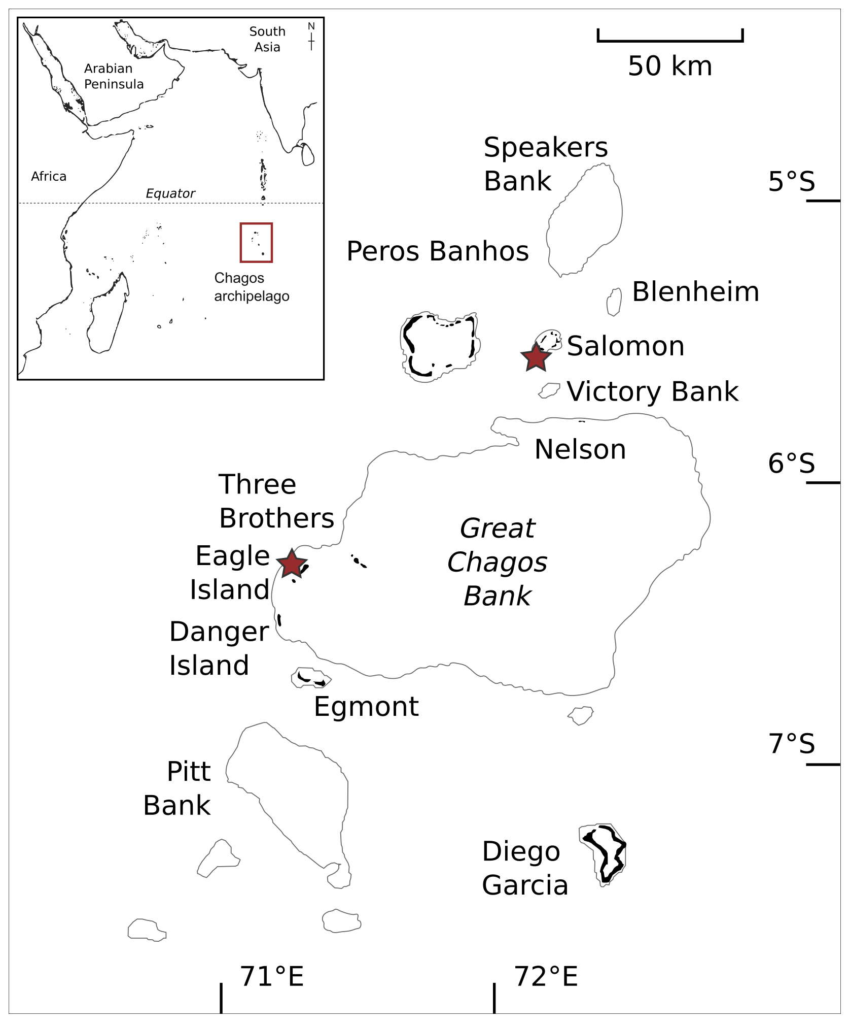
Figure 1 Location of study area and coral sample locations. The Chagos Archipelago is located in the central Indian Ocean, about 550 km south of the Maldives (map upper left). Fossil coral samples were collected on Eagle Island and on Boddam Island (Salomon Atoll; red stars).

2.2 Climate

Chagos is situated in a region characterized by a monsoon climate (Sheppard et al., 2012). The northeast monsoon in austral summer is the wet season, and it lasts from October to February (Pfeiffer et al., 2004). Light to moderate northwest trade winds blow. From April to October, strong winds from the southeast dominate (Sheppard et al., 1999).

Chagos lies at the eastern margin of the so-called Seychelles–Chagos thermocline ridge (SCTR). In the SCTR, a shallow thermocline causes open-ocean upwelling of cold waters. Upwelling along this region was first identified by McCreary et al. (1993) and is forced by both negative and positive wind stress curl (Hermes and Reason, 2009; McCreary et al., 1993). Compared with other upwelling regions in the Indian Ocean, the SSTs of the SCTR are relatively high (between 28.5 and 30 ^∘C in austral summer). This causes very strong air–sea interactions (e.g., Hermes and Reason, 2008; Vialard et al., 2009).

On interannual timescales, the dominant mode of climate variability in the SCTR is the El Niño–Southern Oscillation (ENSO). During El Niño events, the West Pacific warm pool is displaced towards the east resulting in cooler than normal SSTs in the western Pacific and basin-wide warming of the Indian Ocean (Izumo et al., 2014; Sheppard et al., 2013). Figure 2 compares the positive SST anomalies during El Niño events with the negative SST anomalies during La Niña events in the Indian and Pacific oceans between 1982 and 2016, as inferred from “Reynolds” OI v2 SST data (Reynolds et al., 2002; averaged over December–February). An ENSO response in the tropical Indian Ocean can be observed. However, this response is not as strong as it is in the Pacific Ocean.

Figure 2 Composite maps of SST anomalies [^∘C] in the Indian and Pacific oceans during El Niño and La Niña events. (a) El Niño SST anomalies for the period from 1982 to 2016 averaged over December to February. Panel (b) is the same as panel (a) but for La Niña events. SST anomaly maps were computed with NOAA “Reynolds” OI v2 SST (Reynolds et al., 2002) using the free Data Views web application from the IRI Data Library (available at: https://iridl.ldeo.columbia.edu/, last access: 17 September 2018; IRI/LDEO, 2018). Red squares indicate the location of the study area. An overview of all events used for each composite map can be found in Table S1 in the Supplement.

Coupled ocean–atmosphere instabilities centered in the tropical Indian Ocean result in Indian Ocean Dipole (IOD) events (Saji et al., 1999; Sheppard et al., 2013; Webster et al., 1999). A negative (positive) IOD event is defined by warmer (cooler) than normal SSTs in the eastern part of the Indian Ocean and cooler (warmer) than normal SSTs in the western Indian Ocean. Several studies showed that the IOD is an inherent mode of variability of the Indian Ocean (e.g., Ashok et al., 2003; Krishnaswamy et al., 2015; Saji et al., 1999; Webster et al., 1999). The instrumental record of past IOD events does not go back further than 1960 (Saji and Yamagata, 2003). Coral-based reconstructions of past IOD events covering the past millennium suggest a recent intensification of the IOD (Abram et al., 2008, 2020). Those corals show few strong IOD events (i.e., 2019, 1997/1998, 1961, 1877/1878, and 1675), of which only three events (2019, 1961, and 1675) occur independently of ENSO. Considering that an anomaly event recorded by corals can indicate both positive and negative IOD and El Niño and La Niña events, respectively, and that both phenomena tend to occur together (e.g., Luo et al., 2010; Saji and Yamagata, 2003), we decided to treat positive SST anomaly events found in our records as El Niño events even if they could be a result of IOD events independent of or co-occurring with El Niño and La Niña events.

2.3 Instrumental data

Analysis of SST determined from the Advanced Very High Resolution Radiometer (AVHRR) satellite SST product (Casey et al., 2010) for the varying grid areas in Chagos – open ocean (7.13–7.63^∘ S, 72.13–72.63^∘ E) and lagoon (5.13–5.63^∘ S, 71.63–72.13^∘ E) – reveals different SST seasonality at Chagos depending on the reef setting (Fig. 3; cf. Leupold et al., 2019). At the open-ocean reefs, where upwelling occurs, seasonal minima in SSTs are colder than in the lagoon, whereas maximum temperatures are not significantly different (t value =0.27; p value =0.79). Averaged over the entire area of the Chagos Archipelago (4–8^∘ S, 70–74^∘ E), SSTs are similar to SSTs measured in the lagoon. Long-term monthly SST anomalies (i.e., mean seasonal cycle removed) reveal that interannual SST anomalies, such as the El Niño event in 1997/1998 or the La Niña event in 2010/2011, have the same magnitude in both lagoon and open-ocean settings (Fig. 3b). Both anomaly records are not significantly different (t value =0.34; p value =0.37). This suggests that the magnitudes of interannual signals at Chagos should be recorded consistently in all coral records analyzed in this study.

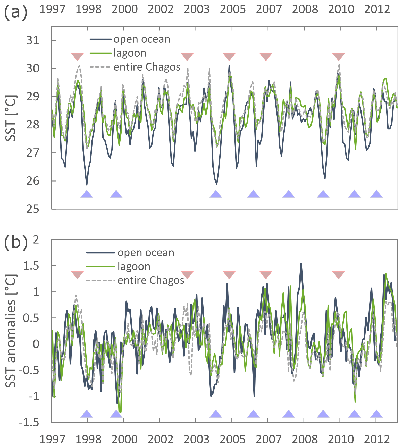
Figure 3 Satellite SSTs for different settings (lagoon: green; open ocean: dark blue) and the entire Chagos Archipelago (gray; averaged over the region from 4 to 8^∘ S and from 70 to 74^∘ E). (a) Monthly satellite SST means and (b) satellite SST anomalies. For the open-ocean and lagoon setting we used the high-resolution satellite SST product AVHRR (Casey et al., 2010), and for the entire Chagos Archipelago we used NOAA “Reynolds” OI v2 SST (Reynolds et al., 2002). Triangles indicate El Niño (red) and La Niña events (blue) based on Brönnimann et al. (2007) and the oceanic Niño index ONI (available at: https://www.ggweather.com/enso/oni.htm, last access: 18 October 2018; El Niño and La Niña Years and Intensities, 2018).

2.4 ENSO indices

The instrumental record of past El Niño and La Niña events is restricted to the late-19th and early-20th centuries. Reconstructions of past ENSO events differ depending on the statistics and/or proxies used (see, e.g., Wilson et al., 2010, and Brönnimann et al., 2007, for a discussion). Therefore, we compare our coral data with different ENSO indices presented briefly in the following. The study of Wilson et al. (2010) reconstructed an annually resolved Niño 3.4 index of past El Niño and La Niña events back to 1607, beyond the instrumental era, using data from the central Pacific (corals), the Texas–Mexico region of the USA (tree rings) and other regions in the tropics (corals and an ice core), which we will refer to as the “Wilson Niño index”. We use the Wilson Niño index for comparison with our coral SST records performing wavelet coherence analysis in the time domain (see Sect. 4.4). Data on the occurrence and magnitude of historical El Niño and La Niña events have been taken from Brönnimann et al. (2007). They combined several reconstructed ENSO indices, climate field reconstructions, and early instrumental data, which were evaluated for consistency. Their reconstruction period extends back to 1500 (La Niña events) and 1511 (El Niño events), respectively. We also include the classical ENSO reconstruction of Quinn (1993) based on historical observations of various aspects of ENSO, which extends back until 1500. Both records (Brönnimann et al., 2007; Quinn, 1993) cover all our coral time windows, including our 17th century coral record. By including the original list of Quinn (1993), alongside the updated list of Brönnimann et al. (2007), we aim to evaluate the sensitivity of our analysis to different ENSO reconstructions. We use both indices by Brönnimann et al. (2007) and Quinn (1993) for identifying past warm and cold events in each coral record that we then use to compile composites (see Sect. 4.5).

3 Methods and materials

3.1 Coral collection and preparation

For this study, three sub-fossil coral samples were collected from boulder beaches and derelict buildings of former settlements at Chagos in February 2010 (Fig. S1). The sub-fossil corals record 41 years of a period from the mid-Little Ice Age (1675–1716), which coincides with the Maunder Minimum, a period of reduced sunspots observations (Eddy, 1976), 31 years of the late Little Ice Age (1836–1867), and 39 years of the mid-19th to early-20th century (1870–1909). Samples E3 (1870–1909) and E5 (1675–1716) were taken from Eagle Island (S 6^∘11.39^′; E 71^∘19.58^′), an island located on the western rim of the Great Chagos Bank (Fig. 1). Sample B8 (1836–1867) was taken from the lagoon-facing sampling site of Boddam Island (S 5^∘21.56^′; E 72^∘12.34^′) in the southwestern part of the Salomon Atoll. The samples were cross-sectioned into 0.7–1.0 cm thick slabs and X-rayed with a Faxitron X-ray model 43885 operated at 50 keV for 1–2 min and used together with a Konica Minolta Regius ∑ RC 300 reader. From the slabs of each sub-fossil coral, powder samples were drilled at 1 mm increments using a micro-milling machine (type PROXXON FF 500 CNC). This depth resolution can be translated to a monthly temporal resolution with average growth rates of 12 mm yr⁻¹. The subsampling paths were always set along the optimal growth axis that was determined based on X-ray images (Fig. S2).

Core GIM, a modern coral core, was included in the coral composite of the SCTR (Pfeiffer et al., 2017). This composite comprises cores from the Seychelles and Chagos. Additionally, the core top (1950–1995) of the GIM core has been calibrated with SST (Pfeiffer et al., 2009). Core GIM was drilled underwater in 1995 in the lagoon of Peros Banhos, located in the northwest of Chagos, from a living coral colony. The monthly coral Sr∕Ca record of GIM extends from 1880 to 1995. Analytical procedures have been described in Pfeiffer et al. (2009). In this study, we use this core to estimate the magnitude of modern El Niño and La Niña events.

3.2 Coral Sr∕Ca analysis

Sr∕Ca measurements were performed at Kiel University using a Spectro Ciros CCD SOP (coupled device chips standard operating procedure) inductively coupled plasma optical emission spectrometer (ICP-OES) following a combination of techniques described by Schrag (1999) and de Villiers et al. (2002). Elemental emission signals were simultaneously collected and subsequently drift corrected by sample–standard bracketing every six samples. Between 0.13 and 0.65 mg of coral powder was dissolved in 1.00 mL 0.2 M HNO₃. Before analysis, the solution was diluted with 0.2 M HNO₃ to a final concentration of approximately 8 ppm calcium. Strontium and calcium intensity lines used are 421 and 317 nm, respectively. The intensities of strontium and calcium were converted into Sr∕Ca ratios in millimole per mole (mmol/mol). Before and after each measurement sequence (n=448 measurements), a stack of eight different reference materials, including international reference materials, JCp-1, and JCt-1 (Hathorne et al., 2013), were measured and used for calibration. For drift correction, an in-house coral reference standard (Mayotte coral) was used. The average analytical precision of Sr∕Ca determinations is 0.08 % relative standard deviation (RSD) or 0.008 mmol mol⁻¹ (n=1973), translating into a temperature of around 0.1 ^∘C. The reproducibility of Sr∕Ca ratios from multiple measurements both on the same day and on consecutive days is 0.08 % RSD (n=238; 1SD), translating into a temperature uncertainty of around 0.1 ^∘C.

3.3 Chronology

Each sub-fossil coral sample was dated by U–Th in 2016. U–Th isotopic measurements were performed with a multicollector-inductively coupled plasma mass spectrometer (MC-ICP-MS; Thermo Electron Neptune) in the High-Precision Mass Spectrometry and Environment Change Laboratory (HISPEC) of the Department of Geosciences, National Taiwan University (NTU), following techniques described in Shen et al. (2012). U–Th isotopic compositions and concentrations are listed in Table 1.

Table 1 Overview of uranium and thorium isotopic compositions and ²³⁰Th ages and corresponding years for fossil coral samples E5 (1675–1716), B8 (1836–1867), and E3 (1870–1909) measured. Location of measurement numbers are indicated on X-ray images in Fig. S2. Chemical analyses were performed on 11 March 2016 and on 16 July 2017 (Shen et al., 2003), and instrumental analyses were carried out on MC-ICP-MS (Thermo Electron Neptune) at NTU (Shen et al., 2012).

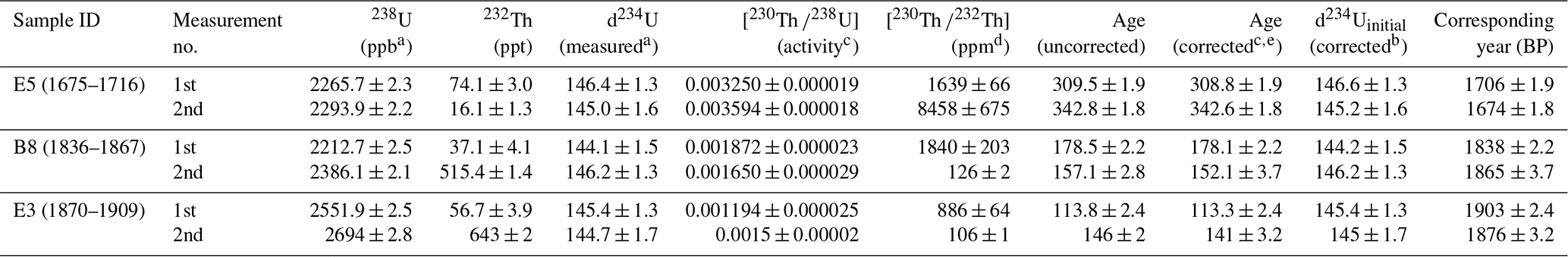
Analytical errors are 2σ of the mean. ^a [²³⁸U] = [²³⁵U] × 137.818 (± 0.65 ‰) (Hiess et al., 2012); ${\mathit{\delta }}^{\mathrm{234}}\mathrm{U}=({[}^{\mathrm{234}}\mathrm{U}{/}^{\mathrm{238}\mathrm{U}}$]_activity−1) × 1000. ^b The δ²³⁴U_initial corrected value was calculated based on the ²³⁰Th age (T), i.e., ${\mathit{\delta }}^{\mathrm{234}}{\mathrm{U}}_{\mathrm{initial}}={\mathit{\delta }}^{\mathrm{234}}{\mathrm{U}}_{\mathrm{measured}}X{e}^{\mathit{\lambda }\mathrm{234}\times T}$, and T is the corrected age. ^c [²³⁰Th∕²³⁸U]${}_{\mathrm{activity}}=\mathrm{1}-e{-}^{\mathit{\lambda }\mathrm{230}T}+({\mathit{\delta }}^{\mathrm{234}}{\mathrm{U}}_{\mathrm{measured}}/\mathrm{1000})[{\mathit{\lambda }}_{\mathrm{230}}$/(λ₂₃₀−λ₂₃₄)]($\mathit{\lambda }-e{-}^{\left(\mathit{\lambda }\mathrm{230}\mathit{\lambda }\mathrm{234}\right)T}$), where T is the age. ^d The degree of detrital ²³⁰Th contamination is indicated by the [²³⁰Th∕²³²Th] atomic ratio instead of the activity ratio. ^e Age corrections, relative to chemistry date, for samples were calculated using an estimated atomic ²³⁰Th∕²³²Th ratio of 4 ± 2 ppm. Those are the values for a material at secular equilibrium, with the crustal ²³²Th∕²³⁸U value of 3.8. The errors are arbitrarily assumed to be 50 %.

Sample E5 covers the period from 1675 to 1716 and is hereafter referred to as E5 (1675–1716); sample B8 covers the period from 1836 to 1867 and is hereafter referred to as B8 (1836–1867); and E3 covers the period from 1870 to 1909 and is hereafter referred to as E3 (1870–1909). The uncertainties of the age models are approximately ± 1.9 years (E5), ± 2.2 years (B8), and ± 2.4 years (E3). All age models were verified by a second, independently measured U–Th age of each sample (measured in 2017 in the HISPEC laboratory of the Department of Geosciences, NTU), following techniques described in Shen et al. (2012). These age determinations are consistent with our Sr∕Ca chronologies.

The chronology of the samples was developed based on seasonal cycles of coral Sr∕Ca and by analyzing the density bands visible on X-ray images (Fig. S2). We assigned the highest Sr∕Ca value to the SST minimum of each year and interpolated linearly between these anchor points to obtain a time series with equidistant time steps.

3.4 Diagenesis screening

A combination of X-ray diffraction (XRD) and optical as well as scanning electron microscopy (SEM) was used to investigate potential diagenetic alteration in the sub-fossil coral samples from Chagos that may have affected the Sr∕Ca values (Figs. S3–S5). Representative samples for diagenesis screening were selected from all corals based on the X-ray images.

For each coral sample, diagenetic modifications were analyzed using one thin section, one sample for SEM, one 2-D XRD measurement and one powder XRD measurement. The Bruker D8 ADVANCE GADDS 2-D XRD system at the Rheinisch-Westfaelische Technische Hochschule (RWTH), Aachen, was used for non-destructive XRD point measurements directly on thin-section blocks with a calcite detection limit of ∼ 0.2 % (Smodej et al., 2015).

3.5 Statistics

All coral Sr∕Ca records were centered, i.e., normalized with respect to their mean values (Pfeiffer et al., 2009), and translated into SSTs using a temperature dependence of −0.06 mmol mol⁻¹ per 1 ^∘C for Porites corals at Chagos (Leupold et al., 2019; Pfeiffer et al., 2009).

Wavelet coherence plots between the coral Sr∕Ca records and the Wilson Niño index were generated using the MATLAB (version R2019b) software toolboxes by Grinstedt et al. (2004) to assess whether the interannual variability recorded in the corals is related to ENSO.

Composites of El Niño and La Niña events were generated by calculating the mean of positive and negative anomaly events taken from centered monthly coral SST anomaly records (see Sect. 4.5). By centering the coral records to their mean and focusing on interannual variability, we eliminate the largest uncertainty of single-core Sr∕Ca records, as shown by Sayani et al. (2019).

The t tests were conducted using the “t test Calculator” free web application (GraphPad QuickCalcs, 2019; available at https://www.graphpad.com/quickcalcs/ttest1/, last access: 9 April 2019). These tests were used to determine if the mean values of two datasets, e.g., mean annual cycles in Sect. 4.3 or mean anomalies of coral composites in Sect. 4.5, are significantly different from each other.

As the significance of the monthly mean anomalies calculated for the composite records depends on the number of events, the standard errors (SEs) for monthly mean anomaly values were used and calculated as follows:

$$\begin{array}{}\text{(1)}& \mathrm{SE}={\displaystyle \frac{\mathrm{standard}\mathrm{deviation}\left(\mathit{\sigma }\right)}{\sqrt{\mathrm{number}\mathrm{of}\mathrm{events}\left(n\right)}}}\end{array}$$

4 Results and Interpretation

4.1 Diagenesis

Only trace amounts of diagenetic phases were detected in the sub-fossil coral samples, which show a good to excellent preservation according to the criteria defined in Cobb et al. (2013). Isolated scalenohedral calcite cement crystals were observed in the thin section of E5 (1675–1716) (Fig. S3a–d). However, XRD results and SEM analysis confirm that the calcite abundance is below the detection limit of XRD (0.2 %) in this sample (Fig. S3e–f). The thin section of B8 (1836–1867) shows trace amounts of patchily distributed, thin aragonite cement (Fig. S4). The thin section of E3 (1870–1909) is devoid of diagenetic phases (Fig. S5), but the dissolution of centers of calcification can be seen in some areas (Fig. S5c–d). Slight dissolution and microborings are also visible with SEM (Fig. S5f). However, microborings are always open and therefore will not influence the geochemistry. In summary, diagenesis screening revealed that the coral samples are suitable for conducting geochemical analysis, and diagenetic modifications to the Sr∕Ca records should be negligible.

4.2 Sr∕Ca measurements

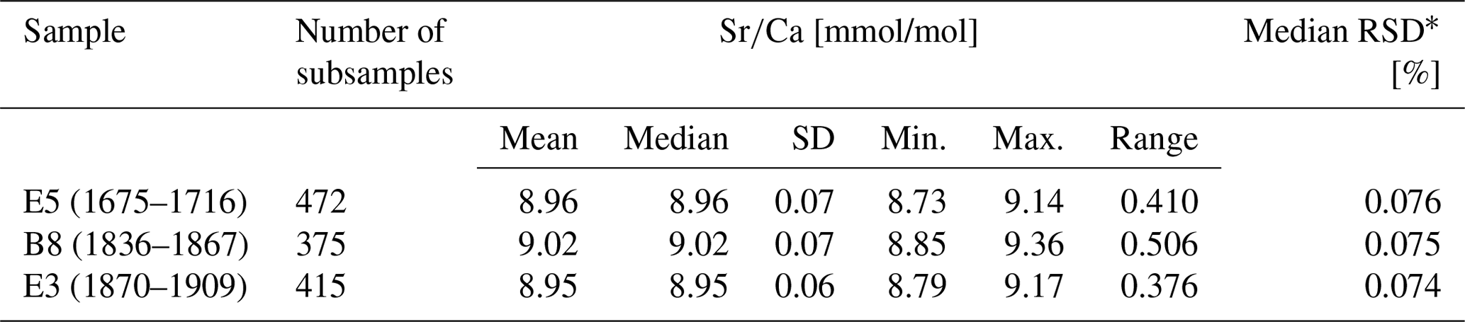
Table 2 gives an overview of the Sr∕Ca ratios of each sub-fossil coral core and statistical key figures of the records. The monthly Sr∕Ca time series are shown in Fig. 4.

Table 2 Statistical overview of raw Sr∕Ca data.

^* RSD is the relative standard deviation.

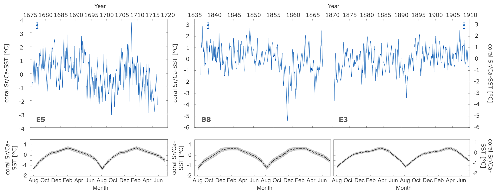
Figure 4 Monthly Sr∕Ca records (blue lines; converted into coral Sr∕Ca–SST in ^∘C) of E5 (1675–1716), B8 (1836–1867), and E3 (1870–1909) with error bars indicating the standard deviation (± 2σ) of Sr∕Ca ratios from multiple measurements on the same day and on consecutive days and mean annual cycles (black lines and corresponding standard errors highlighted in gray, lower plot).

A total of 472 subsamples from E5 (1675–1716) were measured for Sr∕Ca. The average Sr∕Ca value was 8.96 ± 0.07 mmol mol⁻¹. The minimum Sr∕Ca value over the 41-year sample span was 8.73 mmol mol⁻¹, and the maximum value was 9.14 mmol mol⁻¹. From B8 (1836–1867), Sr∕Ca ratios of 375 subsamples were measured. The average value was 9.02 ± 0.07 mmol mol⁻¹. The maximum Sr∕Ca value for the 31-year sample span was 9.36 mmol mol⁻¹, and the minimum Sr∕Ca value was 8.85 mmol mol⁻¹. For E3 (1870–1909), Sr∕Ca measurements were conducted on 415 subsamples. The average Sr∕Ca value was 8.95 ± 0.06 mmol mol⁻¹ for the 39-year sample span, with the minimum value being 8.79 mmol mol⁻¹ and the maximum value being 9.17 mmol mol⁻¹.

The maximum ranges among the corals vary: E5 (1675–1716) has the greatest range and E3 (1870–1909) has the smallest one. It can be seen that mean and median values are the same, i.e., these corals are not biased towards one season. Sample B8 (1836–1867) has a different mean than E5 (1675–1716) and E3 (1870–1909). This underlines the necessity to center the coral records to their mean to eliminate the uncertainty of single-core Sr∕Ca records, as explained in Sect. 3.5.

4.3 Decadal variability and seasonal cycle

All coral SST records show variability on decadal scale (Fig. 4). This variability with a periodicity of 9–13 years has previously been described in studies of Indian Ocean corals (Charles et al., 1997; Cole et al., 2000; Pfeiffer et al., 2006, 2009; Zinke et al., 2008). Within a decadal cool (warm) phase, negative (positive) SST anomalies may occur. In particular, high-amplitude, short-term cool events are possible as Chagos lies in a region where open-ocean upwelling occurs (see Leupold et al., 2019). To ensure that decadal variability does not influence the composite records by inflating interannual warm or cool anomalies, decadal variability is removed by detrending the coral records.

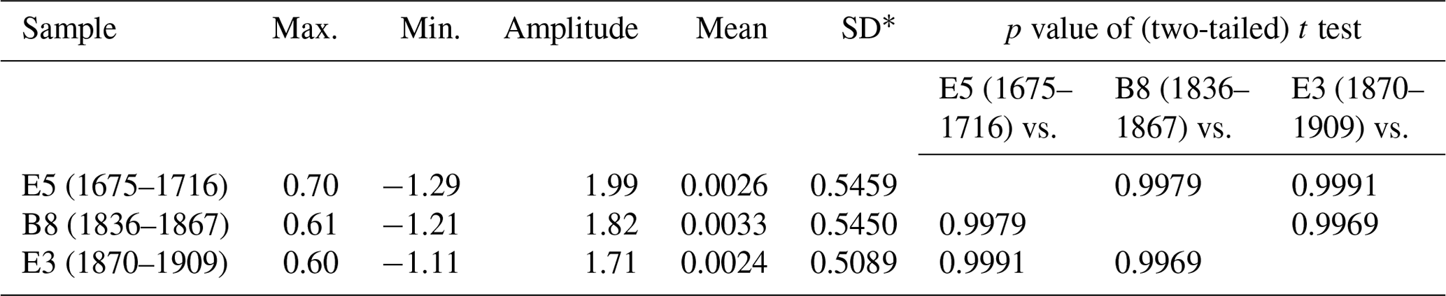
The mean annual cycles of all sub-fossil coral SST records are not significantly different, as indicated by p values of around one in the t tests (Table 3, Fig. 4). The seasonal amplitudes in coral SST (^∘C) are slightly higher in E5 (1675–1716) (1.99 ^∘C) than in B8 (1836–1867) (1.81 ^∘C) and E3 (1870–1909) (1.71 ^∘C). A shift of the seasonal temperature maximum from February (E5 and B8) to April (E3) can be observed (Fig. 4). Seasonal amplitudes explain 26 %–32 % of the coral–SST variance (see in the Supplement and Fig. S6).

Table 3 Statistical overview for mean annual cycle data of the coral Sr∕Ca–SST [^∘C] records.

^* SD is the standard deviation.

4.4 ENSO signals in coral SST records

The modern and the sub-fossil coral SST records were compared with the annually resolved Wilson Niño index that extends back until 1607 (Wilson et al., 2010). All coral records show positive and negative SST anomalies, which occur in years where El Niño and La Niña events have been reported (Fig. 5) and wavelet power spectra show significant interannual variability in the ENSO frequency band (Fig. S7). To analyze a possible correlation between the coral SST records and ENSO, wavelet coherence (WTC) was conducted on all coral records and the Wilson Niño index (Wilson et al., 2010). WTC plots were generated to find regions in time-frequency space where the Wilson Niño index and the Chagos coral SST records covary, even if they do not have high power in those regions (Fig. 6).

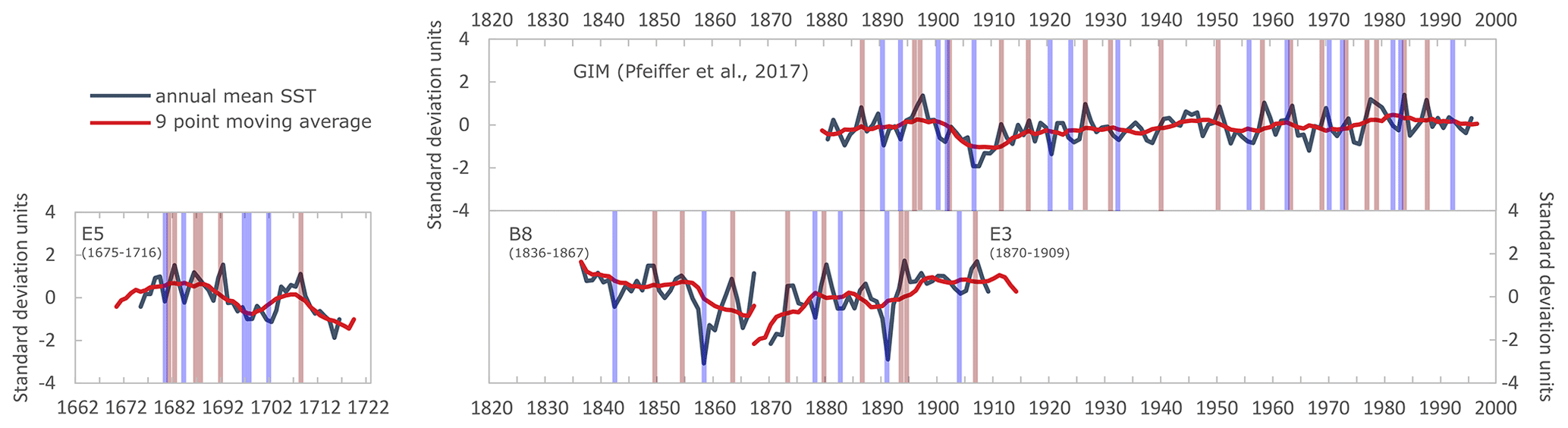
Figure 5 Annual SST anomalies for Chagos corals (this study and core GIM from Pfeiffer et al., 2009, 2017); red indicates El Niño, blue indicates La Niña, and shaded boxes indicate years used for the composite records (Figs. 7–9). Thick red lines are nine-point moving averages. See text Sect. 4.5 for how El Niño and La Niña events were picked.

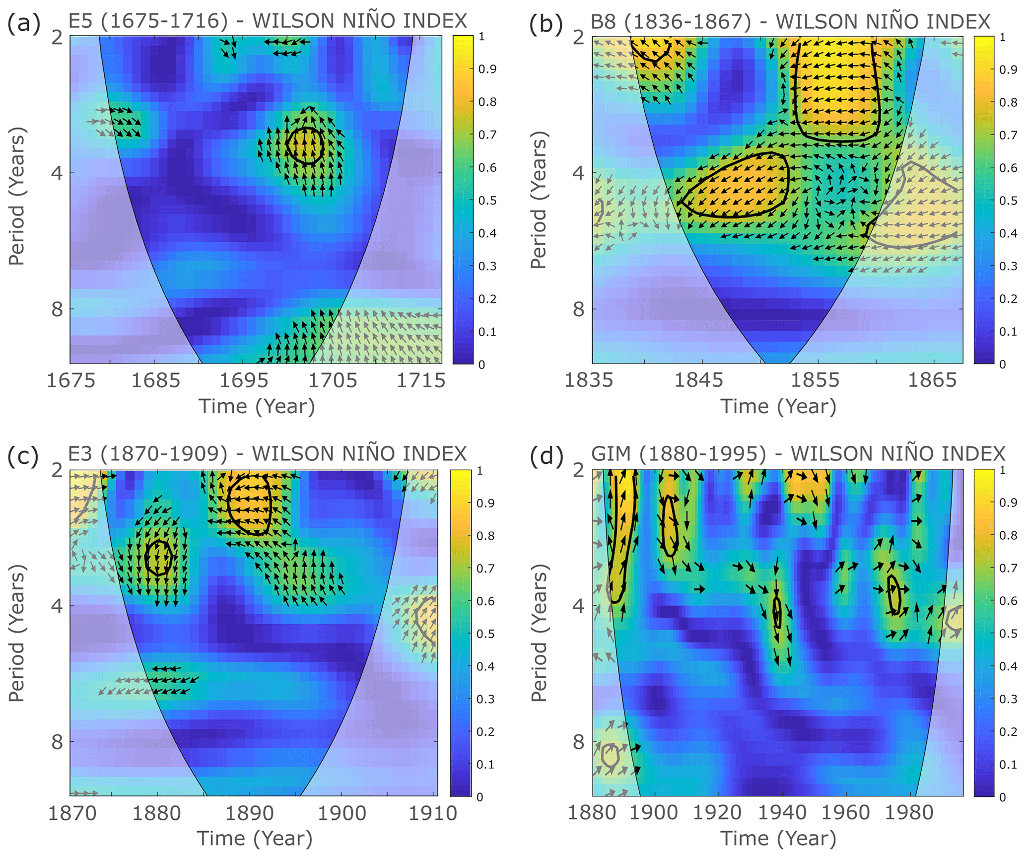
Figure 6 Wavelet coherence analysis plots for the Wilson Niño index (Wilson et al., 2010) and Chagos coral SST of (a) E5 (1675–1716), (b) B8 (1836–1867), (c) E3 (1870–1909), and (d) GIM (1980–1995).

All WTC plots of the Wilson Niño index and coral SST records reveal time-localized areas of strong coherence occurring in periods that correspond to the characteristic ENSO cycles of 2 to 8 years. The WTC plots for the Wilson Niño index and the 19–20th century coral records show several regions where both time series covary. In contrast, the WTC plot of the Wilson Niño index and the 17–18th century coral SST record shows only one region of covariation at the beginning of the 18th century. The plots show that there is an approximate lag of 9 months to 1 year between the 17–18th century coral SST record and the Wilson Niño index (Fig. 6a) and a lag of approximate 1 to 3 years between B8 (1836–1867) and E3 (1870–1909) and the Wilson Niño index, respectively (Fig. 6b, c). However, the lags between the coral SST and the index time series are in the range of the age model uncertainties of the sub-fossil corals and do not represent real time lags. For a further comparison of the coral SST records' and the Wilson Niño index's frequencies, singular spectrum analysis and power spectra of non-detrended and detrended time series were computed (see the Supplement).

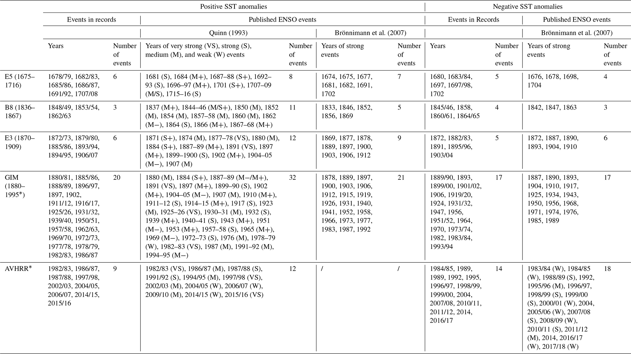
All coral records show anomaly events that can be explained with El Niño and La Niña events listed in Brönnimann et al. (2007) or Quinn (1993; Tables 4–6). Our results show that, compared to the 17–18th century, more El Niño and La Niña events per period are recorded in coral records of the central Indian Ocean during the late 20th century. According to the AVHRR satellite data and coral records, an El Niño event occurs on average every 4 years between 1981 and 2017 (AVHRR) or every 5 years between 1965 and 1995 (coral record), respectively (Tables 4–6). This is supported by the events listed in Quinn (1993) and reflects a change in ENSO frequency in the tropical Pacific. Overall, predominantly strong El Niño events are recorded by the coral records from Chagos, as indicated in the list of events presented in Brönnimann et al. (2007; Table 6). The number of events listed in Brönnimann et al. (2007) is comparable to the number of events recorded in the corals, whereas the number of events listed in Quinn (1993) is higher than the number of events recorded in the corals. The same holds for the negative SST anomaly events (La Niña and non-La Niña events): the number of La Niña events listed in Brönnimann et al. (2007) is similar to the number of negative anomaly events recorded in the coral records. Furthermore, negative anomaly events occurred every 2.6 years in the AVHRR data (1981–2017), every 6 years in the coral record (1965–1995), and every 5 years in Brönnimann et al. (2007; 1965–1995). During the 17–18th century, negative SST anomalies occurred every 6.8 years (coral record) or 10.3 years (Brönnimann et al., 2007; Tables 4–6).

Table 4 Positive (El Niño events) and negative (La Niña events, LN, shown using bold font; and non-La Niña events, NLN, shown using italic font) SST anomaly events picked for generating coral and satellite composite records shown in Figs. 7 and 8.

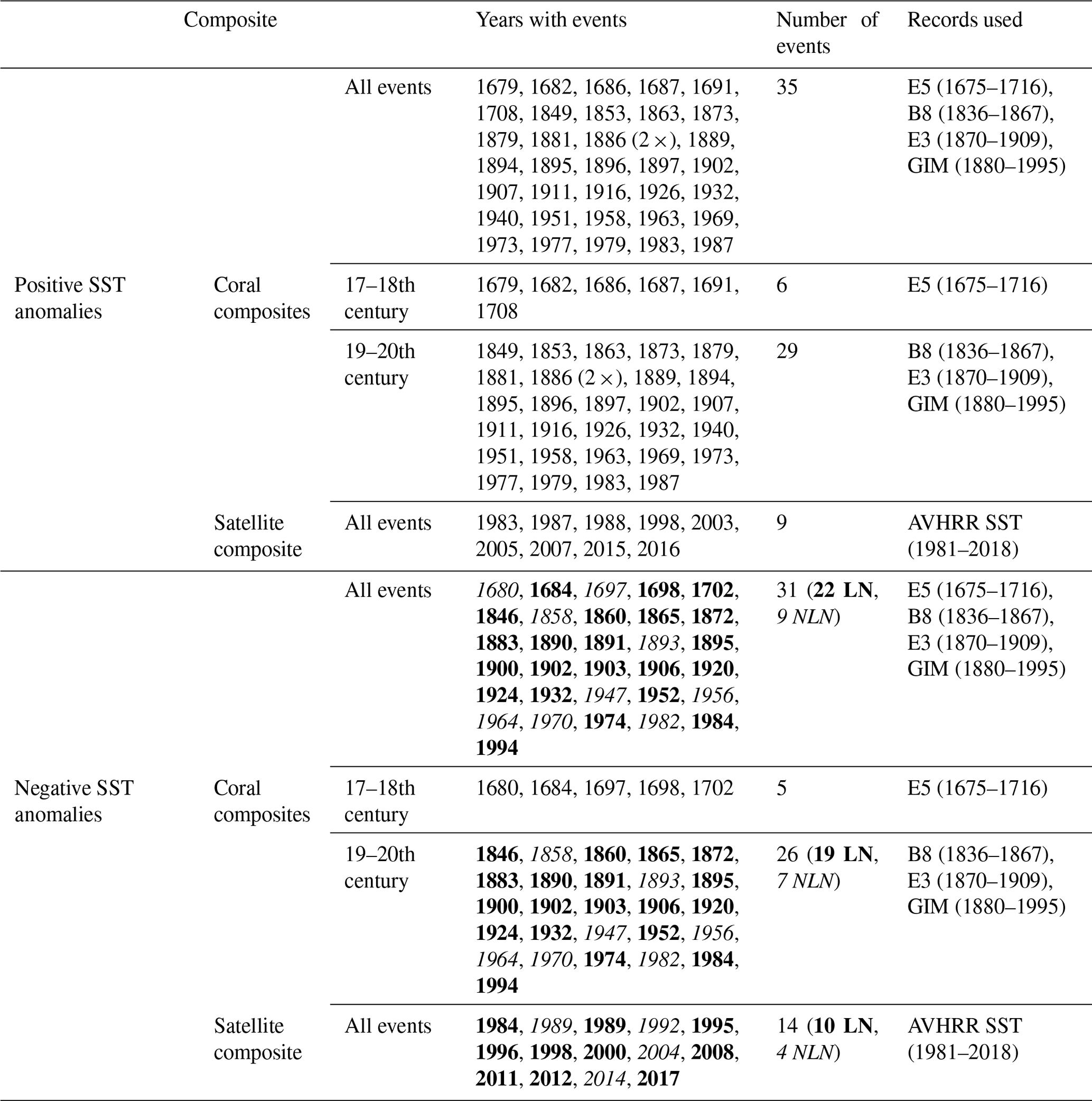
Table 5 The 19–20th century (divided into three periods) positive (El Niño events) and negative (La Niña and non-La Niña events) SST anomaly events picked for generating coral composite records shown in Fig. 9.

Table 6 Overview of all events found in the coral Sr∕Ca records and of El Niño and La Niña events of corresponding time periods listed in publications. Events in coral records were matched with published events in consideration of age model uncertainties of each coral record.

Recent events (from 1980 onward) were additionally picked using events listed on the following website: https://www.ggweather.com/enso/oni.htm (last access: 18 October 2018; El Niño and La Niña Years and Intensities, 2018)

4.5 ENSO composites

Composites of monthly coral SST anomalies were produced for El Niño and La Niña events to assess their magnitudes. Each composite was produced using coral records of several individual El Niño and La Niña events. An overview of the events used for generating each composite can be found in Tables 4 and 5. An overview of all events found in the coral Sr∕Ca records and of El Niño and La Niña events listed in Brönnimann et al. (2007) and Quinn (1993) for the studied time period is given in Table 6. Positive SST anomalies in the coral records were interpreted as El Niño events when (1) the year of occurrence was listed as an El Niño event in Brönnimann et al. (2007) and Quinn (1993) within the error of each coral age model and (2) when the anomaly exceeded 1.5 standard deviations of the mean of each coral record (Fig. S8). In addition to the strong La Niña events listed in Brönnimann et al. (2007), we added negative SST anomalies occurring in years after the El Niño events to the composite.

The composite record for El Niño events comprises 35 events, and 31 events are included in the La Niña composite (Table 4). To investigate changes in the magnitude of ENSO anomalies over time, composites for the respective 17–18th century and 19–20th century time periods were generated. For the 17–18th century, six events (five events) were used for the El Niño (La Niña) composite. The composite for the 19–20th century includes events from the sub-fossil corals and the GIM record. In total, 29 events (26 events) were used for the El Niño (La Niña) composite. These 19–20th century composites, in turn, were split into three subperiods: 1830–1929 (18 El Niño events, 16 La Niña events), 1930–1964 (five El Niño events, five La Niña events; Table 5), and 1965–1995 (six El Niño events, five La Niña events). These subperiods were selected because ENSO activity was reduced between 1930 and 1965 compared with before 1930 and after 1965 (e.g., Cole et al., 1993).

Observations indicate that some upwelling events in the central Indian Ocean are not forced by large-scale ENSO or IOD variability but are associated with cyclonic wind stress curls in the southern tropical Indian Ocean (Dilmahamod et al., 2016; Hermes and Reason, 2009). Such an upwelling event occurred in August 2002 and was found in both the coral and satellite SST records at Chagos (see Leupold et al., 2019).

To investigate the potential effect of such negative anomaly events on the La Niña composites, the 19–20th century composites were split into composites of La Niña events and other negative anomaly events, which were not related to La Niña. La Niña and negative anomalies other than La Niña events were selected based on the months they occurred in, i.e., November–May (La Niña) and June–September (non-La Niña). As such, events are also observed in the satellite era, and we compared modern (1981–2018) satellite SST composites for El Niño events (nine events), La Niña events (10 events), and negative anomalies other than La Niña events (four events) with our coral SST composites. We used the AVHRR satellite SSTs (Casey et al., 2010) averaged over the entire Chagos Archipelago (4–8^∘ S, 70–74^∘ W).

4.5.1 Positive anomalies in coral and satellite SST composites

The central Indian Ocean coral composites of positive SST anomalies reveal higher SST anomalies during El Niño events than the satellite composites (Fig. 7), which may reflect the greater sensitivity of the corals to reef-scale temperatures (Leupold et al., 2019) or the different time periods covered by these records (only two El Niño events in the AVHRR record overlap with the coral data). The coral composite of the 17–18th century shows higher anomalies than the coral composite of the 19–20th century (Fig. 7). All positive SST anomalies identified as El Niño events in the coral records show an average warming of 1.5 ± 0.1 ^∘C (n=35; Fig. 7). The average positive temperature anomaly during El Niño events of the 17–18th century was 2.2 ± 0.2 ^∘C (n=6), which is higher than and significantly different (p ≪ 0.01) from the average positive El Niño temperature anomaly during the 19–20th century (1.3 ± 0.1 ^∘C; n=29). The average positive temperature anomaly of El Niño events picked from the AVHRR satellite SST (covering the period from 1981 to 2018) of 0.8 ± 0.1 ^∘C (n=9) is also lower than and significantly different (p ≪ 0.01) from the average positive El Niño temperature anomaly in the 19–20th century. This suggests a greater impact of El Niño events on the Indian Ocean SST during the 17–18th century compared with the 19–20th century and recent decades.

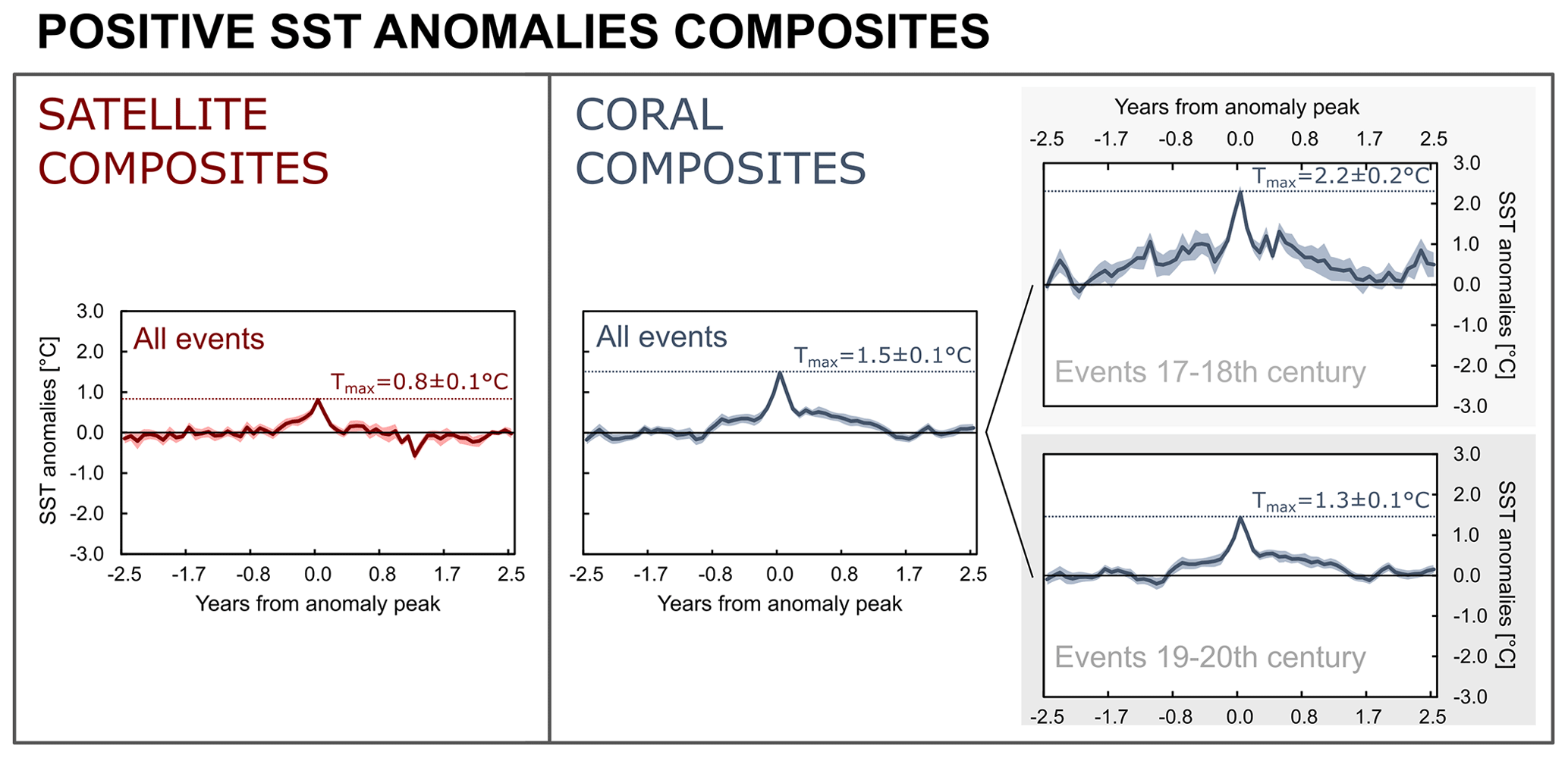
Figure 7 Positive SST anomaly (El Niño events) composite records of AVHRR (left; red) and coral SST (right; blue) records. Separate composites of anomaly events during the 17–18th and 19–20th century were generated from the coral SST records. Shaded areas below and above the curves show the standard error for the mean values of the composite records. See Table 4 for an overview of the events that were selected for generating the composites.

4.5.2 Negative anomalies in coral and satellite SST composites

No statistically significant differences were found between negative anomalies in coral SST in the central Indian Ocean during the 17–18th century and the 19–20th century nor between La Niña and non-La Niña events (Fig. 8).

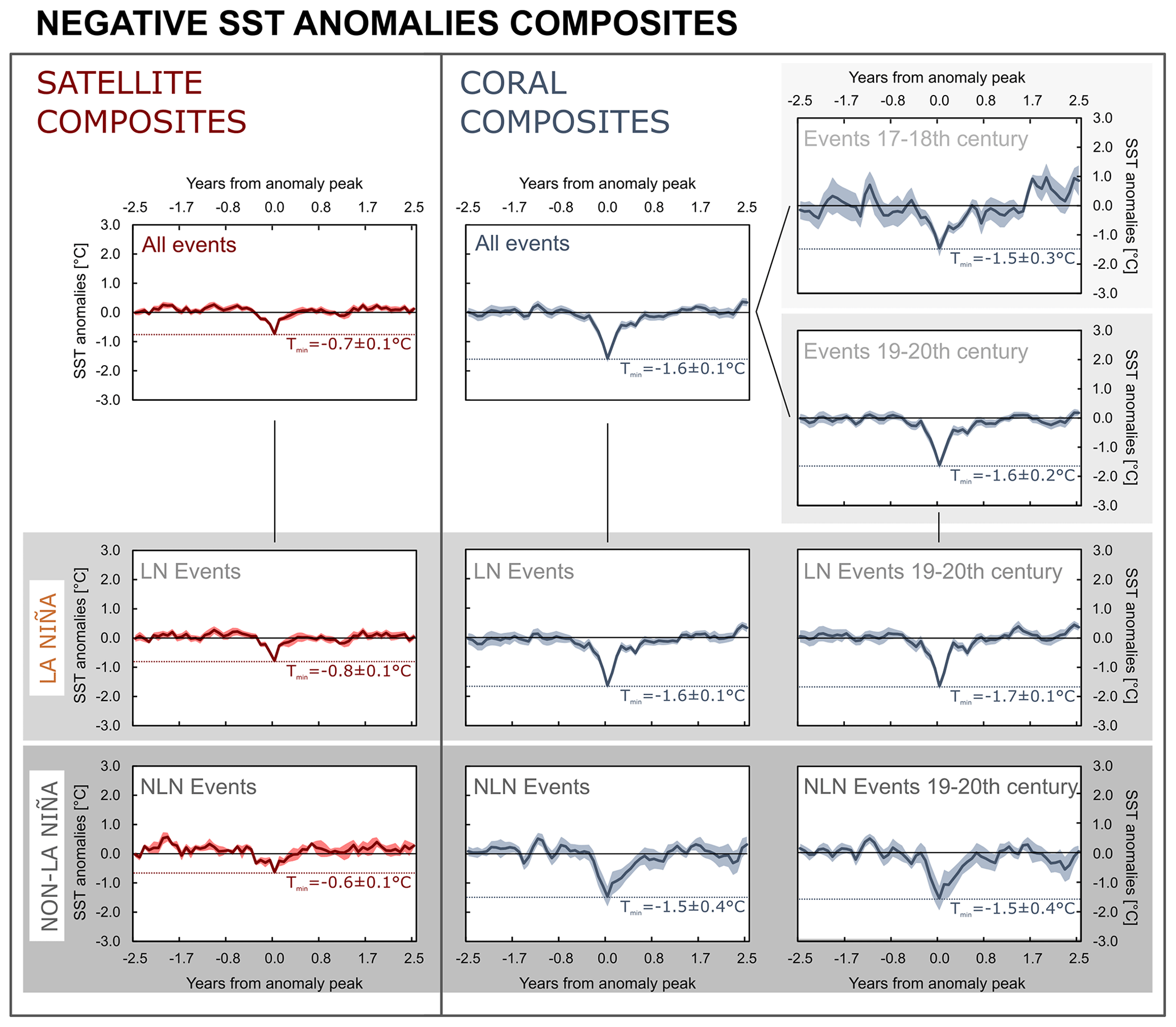
Figure 8 Negative SST anomaly (La Niña and non-La Niña events) composite records of AVHRR satellite (left; red) and coral SST (right; blue) records. Additionally, composites of anomaly events separated by 17–18th and 19–20th century events and by La Niña and non-La Niña events were generated. Shaded areas below and above the curves show the standard error for the mean values of the composite records. See Table 4 for an overview of the events that were selected for generating the composites.

The composite including all negative SST anomalies identified as La Niña and non-La Niña events in the coral records shows an average negative SST anomaly of −1.6 ± 0.1 ^∘C (n=31; Fig. 8). During the 19–20th century, the negative temperature anomaly for all La Niña events is −1.6 ± 0.1 ^∘C (n=22) and for all non-La Niña events it is −1.5 ± 0.4 ^∘C (n=9) (p=0.75). La Niña events are slightly colder than non-La Niña events in the coral composites, but they are not statistically different (p=0.60). The same is observed in the AVHRR satellite SST anomaly composites, where average negative La Niña temperature anomalies are −0.8 ± 0.1 ^∘C (n=10) and non-La Niña anomalies are −0.6 ± 0.1 ^∘C (n=4; p=0.17).

The average negative temperature anomalies of La Niña and non-La Niña events during the 17–18th century were slightly less negative (−1.5 ± 0.3 ^∘C; n=5), but they were not significantly different (p=0.73) from the average negative temperature anomalies of the 19–20th century (−1.6 ± 0.2 ^∘C; n=26).

4.5.3 Interannual SST anomalies during the 19th and 20th century

Dividing the 19–20th century into three subperiods (1830–1929, 1930–1964, and 1965–1995) and compiling SST anomaly composites allowed us to assess changes in the magnitude of ENSO-driven warm and cold anomalies over time (Fig. 9). The El Niño composites do not show systematic changes during the 19–20th century in the Indian Ocean. For the period between 1830 and 1929, the average positive temperature anomaly is 1.4 ± 0.1 ^∘C (n=18); between 1930 and 1964, the average positive temperature anomaly of 1.2 ± 0.1 ^∘C (n=5) is slightly lower than in the previous period but not significantly different (p=0.5). For the last period of the 20th century, 1965 to 1995, the average positive temperature anomaly is again 1.4 ± 0.1 ^∘C (n=6; Fig. 9).

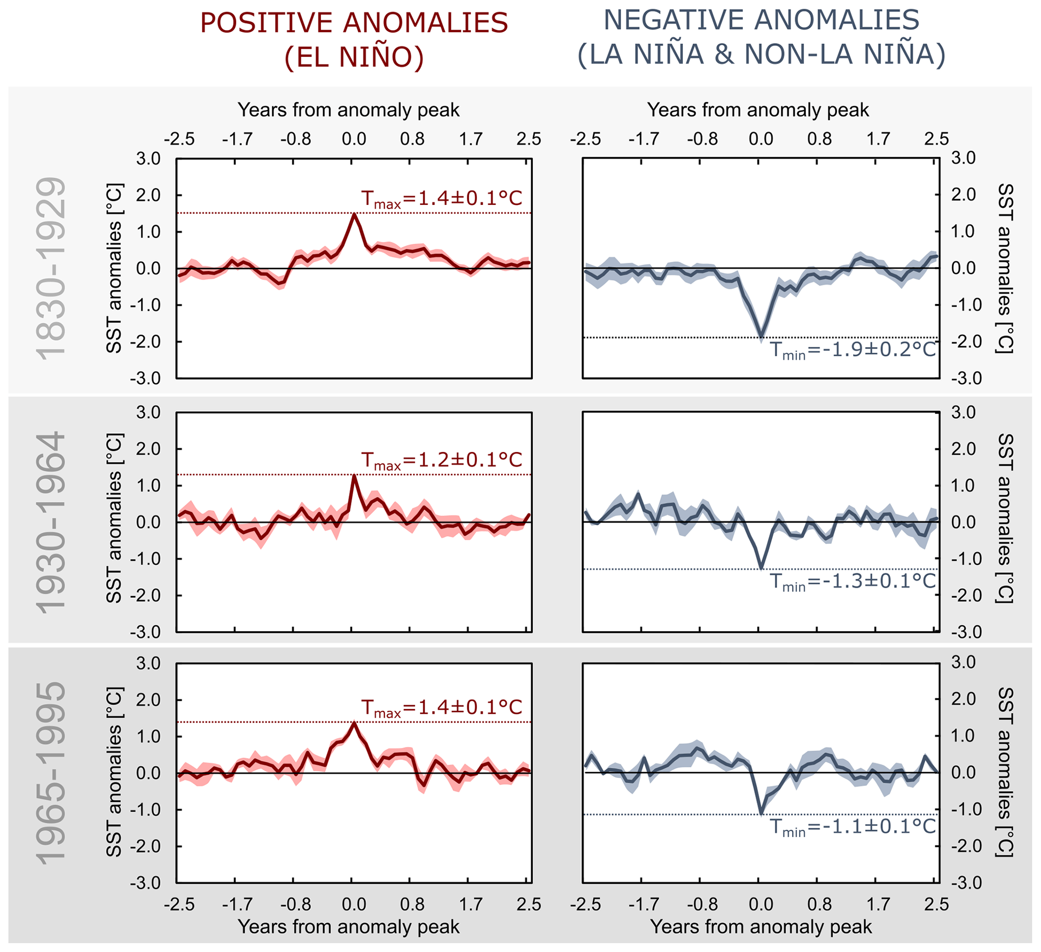
Figure 9 Positive (El Niño events; left) and negative SST anomaly (La Niña and non-La Niña events; right) composite records of the 19–20th century coral SST records separated by the 1830–1929 (top row), 1930–1964 (middle row), and 1965–1995 (bottom row) time intervals. Shaded areas below and above the curves show the standard error for the mean values of the composite records. See Table 5 for an overview of the events that were selected for generating the composites.

The magnitude of cooling during La Niña and non-La Niña events tends to reduce from 1830–1929 to 1965–1995 (Fig. 9). For the period between 1830 and 1929, the average negative temperature anomaly is −1.9 ± 0.2 ^∘C (n=16). Between 1930 and 1964 the average negative temperature anomaly increases by 0.58 ^∘C to −1.3 ± 0.1 ^∘C (n=5), and from 1965 to 1995, the average negative temperature anomaly is −1.1 ± 0.1 ^∘C (n=5). However, for both El Niño and La Niña events, the differences between the means of the first period (1830–1929) and the last period (1965–1995) are not statistically significant (p=0.93 and p=0.07, respectively).

5 Discussion

Previous studies have shown that Indian Ocean SST variability was influenced by ENSO during the 19th and 20th centuries (Charles et al., 1997; Cole et al., 2000). During this period there was a stationary ENSO–SST teleconnection, in the sense that El Niño warmed the Indian Ocean and La Niña cooled it (Pfeiffer and Dullo, 2006). In this study, we show that interannual SST variability recorded in the 17–18th and 19–20th century corals is coherent with the Wilson Niño index. This demonstrates a stationary ENSO–SST teleconnection in the central Indian Ocean since 1675.

Our ENSO composites allow us to estimate and compare the magnitudes of ENSO-induced warming and cooling in the central Indian Ocean. This enables us to assess the symmetry or asymmetry of the ENSO teleconnection, thereby taking the analysis of the ENSO–SST teleconnection one step further. The composites suggest the ENSO teleconnection in the tropical Indian Ocean was close to symmetric, because magnitudes of El Niño and La Niña events recorded by the Chagos corals during the past century are generally comparable (Fig. 9). Only in times of cooler mean climates (i.e., during the 17–18th century) do the corals seem to indicate higher amplitude ENSO-induced warm anomalies in the tropical Indian Ocean, although these differences are not statistically significant. Hence, our results do not support the notion that an asymmetric ENSO teleconnection with strong warming during El Niño years drives the recent warming of the tropical Indian Ocean as suggested by Roxy et al. (2014).

The modern coral records from the central Indian Ocean all show steady warming during the 20th century, and this warming also continues in the period of reduced ENSO activity between 1930 and 1965 (e.g., Abram et al., 2016; Charles et al., 1997; Pfeiffer and Dullo, 2006). This suggests that neither the magnitude nor the frequency of past El Niño events explain the centennial-scale warming of the Indian Ocean.

Previous studies classified El Niño and La Niña events (Tables 4 and 5) qualitatively, from “weak” to “very strong” (Brönnimann et al., 2007; Quinn, 1993; Table 6). All positive anomaly events recorded by the coral records presented in our study were identified in at least one of these two studies (Table 6). However, not every event listed in Brönnimann et al. (2007) and Quinn (1993) is recorded by the central Indian Ocean corals. Specifically, the number of events presented in Quinn (1993) is higher than the number of events recorded by the corals. In contrast, the number of events listed in Brönnimann et al. (2007) is similar to the number recorded by the corals (Table 6). Brönnimann et al. (2007) only listed strong events. This suggests that corals from the central Indian Ocean predominantly record strong events. As most ENSO reconstructions consistently record strong events (while weak to moderate events differ between reconstructions), our results do not depend on the choice of the ENSO reconstruction.

Our results show that El Niño events resulted in stronger SST anomalies in the central Indian Ocean during a cooler mean climate (i.e., during the 17–18th century). This is consistent with Zinke et al. (2004), who found the highest amplitude of interannual variations in the ENSO frequency band between 1645 and 1715 in a coral δ¹⁸O record from Ifaty, Madagascar. To date, the Ifaty coral is the longest continuous coral record from the Indian Ocean with subseasonal resolution. Furthermore, these results are in line with a multi-core study of Pfeiffer et al. (2017). They also found larger amplitudes of ENSO-induced warm anomalies in the tropical Indian Ocean in the late 19th century – a time when mean SSTs in the tropical Indian Ocean were cooler than today.

Comparing both periods (17–18th and 19–20th century), the La Niña and non-La Niña cold events show no significant changes. This suggests a stable negative SST anomaly pattern in the Indian Ocean. There is ambiguity about the reason for this observation. However, the Indian Ocean is the warmest tropical Ocean, and its warmest waters tend to show a low spatial and temporal SST variability. In the western and central Indian Ocean, SSTs in the cold season show the strongest warming since 1900 (e.g., Leupold et al., 2019; Roxy et al., 2014) but also larger spatial and temporal SST variability at various scales (Leupold et al., 2019).

The corals from Chagos record upwelling events in boreal summer, which are independent of ENSO, poorly represented in satellite data of SST (see Leupold et al., 2019), and may result in the failure of the Indian monsoon. Such an upwelling event occurred, for example, in 2002 and led to a drought over the Indian subcontinent (Jayakumar and Gnanaseelan, 2012; Krishnan et al., 2006). At present, little is known about the frequency or magnitude of these events in past decades or centuries. Thus, coral proxy data from Chagos allow us to better understand these non-La Niña upwelling events.

In contrast to the stationary teleconnection between ENSO and SST in the central Indian Ocean, previous studies have shown that the ENSO–precipitation teleconnection is non-stationary (Timm et al., 2005). The impact of ENSO on rainfall in the central Indian Ocean depends on mean SSTs, and these surpassed a critical threshold for atmospheric convection in the mid-1970s, strengthening the El Niño signal in rainfall. However, our study does not indicate an increase in the magnitude of El Niño-related SST anomalies following this shift compared with earlier time periods of strong ENSO activity.

This study confirms that the ENSO–SST teleconnection between the Pacific and the Indian Ocean has been stationary since 1675 and that it is possible to reconstruct the magnitude of interannual SST variations in the tropical Indian Ocean. This is of importance because there currently is no reliable high-resolution reconstruction of ENSO variability in the tropical Indian Ocean covering the periods investigated within this study. ENSO reconstructions from the equatorial Pacific cover the 20th century (1998 to 1886) (Cobb et al., 2001) and time windows from the past millennium: 928–961, 1149–1220, 1317–1464, and 1635–1703 (Cobb et al., 2003). Cobb et al. (2003) combined three overlapping coral records of the 14–15th century and five coral records of the 17–18th century. We have shown that this approach would be applicable to the tropical Indian Ocean as well, using sub-fossil corals from boulder beaches and historical buildings. If a more complete record of millennial-scale coral reconstructions from the tropical Pacific and the Indian Ocean becomes available, it will be possible to assess the ENSO teleconnection based on an analysis of the coral records from both oceans. This is important because recent studies have shown that the tropical Indian Ocean plays a pivotal role in the 20th century global temperature rise (Funk et al., 2008; Pfeiffer et al., 2017; Roxy et al., 2014) and that the processes driving this warming are not yet fully understood.

6 Conclusions

We have shown that the ENSO–SST relationship in the central Indian Ocean has been stationary since the 17th century. All four studied coral records show interannual variability coherent with ENSO variability as well as variations in the intensity of El Niño and La Niña-induced SST anomalies in the central Indian Ocean. El Niño events cause average positive anomalies of 2.2 ± 0.2 ^∘C (n=6) during the 17–18th century and 1.3 ± 0.1 ^∘C (n=29) during the 19–20th century, whereas La Niña events cause average negative anomalies of −1.5 ± 0.3 ^∘C (n=5) during the 17–18th century and −1.6 ± 0.2 ^∘C (n=26) during the 19–20th century in the central Indian Ocean. However, not all cooling events are related to La Niña events, with processes internal to the Indian Ocean also causing negative anomalies of −1.5 ± 0.4 ^∘C (n=7) during the 19–20th century. The magnitudes of El Niño and La Niña events during the last century are comparable, indicating a symmetric ENSO teleconnection. An asymmetric ENSO teleconnection being the cause for the overall warming of the central, tropical Indian Ocean therefore appears unlikely. However, we suggest compiling composite records of negative and positive SST anomaly events from additional sub-fossil Indian Ocean corals to further explore the ENSO–SST teleconnection and how it varies spatially in cooler or warmer climatic intervals.