the Creative Commons Attribution 4.0 License.
the Creative Commons Attribution 4.0 License.
 | 14 Jun 2021
The role of land cover in the climate of glacial Europe
Patricio Velasquez
Jed O. Kaplan
Martina Messmer
Patrick Ludwig
Christoph C. Raible
Earth system models show wide disagreement when simulating the climate of the continents at the Last Glacial Maximum (LGM). This disagreement may be related to a variety of factors, including model resolution and an incomplete representation of Earth system processes. To assess the importance of resolution and land–atmosphere feedbacks on the climate of Europe, we performed an iterative asynchronously coupled land–atmosphere modelling experiment that combined a global climate model, a regional climate model, and a dynamic vegetation model. The regional climate and land cover models were run at high (18 km) resolution over a domain covering the ice-free regions of Europe. Asynchronous coupling between the regional climate model and the vegetation model showed that the land–atmosphere coupling achieves quasi-equilibrium after four iterations. Modelled climate and land cover agree reasonably well with independent reconstructions based on pollen and other paleoenvironmental proxies. To assess the importance of land cover on the LGM climate of Europe, we performed a sensitivity simulation where we used LGM climate but present-day (PD) land cover. Using LGM climate and land cover leads to colder and drier summer conditions around the Alps and warmer and drier climate in southeastern Europe compared to LGM climate determined by PD land cover. This finding demonstrates that LGM land cover plays an important role in regulating the regional climate. Therefore, realistic glacial land cover estimates are needed to accurately simulate regional glacial climate states in areas with interplays between complex topography, large ice sheets, and diverse land cover, as observed in Europe.
- Article
(11173 KB) - Full-text XML
- BibTeX
- EndNote


The Last Glacial Maximum (LGM, 21 ka; Yokoyama et al., 2000; Clark et al., 2009; Van Meerbeeck et al., 2009) is a period of focus for Earth system modelling because it represents a time when boundary conditions were very different from the present and is therefore a good test bed of models' ability to faithfully reproduce a range of climate states (e.g. Mix et al., 2001; Janská et al., 2017; Cleator et al., 2020). In Europe, the LGM is also an interesting period in human history because small groups of highly mobile Upper Paleolithic hunter-gatherers persisted in the face of inhospitable climate, while Neanderthals disappeared (Finlayson, 2004; Finlayson et al., 2006; Finlayson, 2008; Burke et al., 2014; Maier et al., 2016; Baena Preysler et al., 2019; Klein et al., 2021). However, despite more than 3 decades of research, the LGM climate of the continents is only poorly understood. Global climate models (GCMs) show little agreement in LGM simulations for Europe (Braconnot et al., 2012; Kageyama et al., 2017; Ludwig et al., 2019; Kageyama et al., 2021). It has been suggested that a reason for the large uncertainty could be related to the spatial resolution in the climate models (Walsh et al., 2008; Jia et al., 2019b; Ludwig et al., 2019; Raible et al., 2020). Advances in regional climate models have led to the application of such models to the glacial climate of Europe on a high spatial resolution (e.g. Kjellström et al., 2010; Strandberg et al., 2011; Gómez-Navarro et al., 2012, 2013; Ludwig et al., 2017, 2020). Here, we further investigate the importance of land cover for climate during this period.
Paleoclimate reconstructions suggest that the climate of Europe was 10 to 14 ∘C colder and around 200 mm yr−1 drier during the LGM compared to the present day (PD; Wu et al., 2007; Bartlein et al., 2011). However, uncertainties in the paleoclimate reconstructions are large, the few sites with samples dating to the LGM are not uniformly distributed in space (e.g. Wu et al., 2007), and in some regions, reconstructions are contradictory (e.g. de Vernal et al., 2006). For example, some LGM climate reconstructions suggest that the Iberian Peninsula was dry (Bartlein et al., 2011; Cleator et al., 2020), while others suggest wetter conditions were prevalent (Vegas et al., 2010; Moreno et al., 2012). Some of these discrepancies may result from the fact that many paleoclimate archives record a certain season, while the signal is frequently interpreted as an annual value (Beghin et al., 2016), or from the fact that even sites that are close together record strong climatic gradients. Whatever the case, generation of a spatially continuous map of climate and environmental conditions in the LGM Europe is currently not possible using a strictly proxy-driven approach. As an alternative, it should be possible to generate continuous maps using climate models.
GCM simulations are overall consistent with reconstructions in simulating an LGM climate that is largely colder and drier than PD (e.g. Ludwig et al., 2016; Hofer et al., 2012a). At the regional scale, however, GCMs show broad intermodel variety and partly disagree in comparison to proxy reconstructions, particularly concerning the magnitude and spatial patterning of temperature and precipitation (Harrison et al., 2015). For example, GCMs show a broad disagreement in the simulation of precipitation over the Iberian Peninsula, with some models suggesting it was wetter while in others the simulated climate is drier compared to PD (Beghin et al., 2016). One possible explanation for the disagreement is the coarse spatial resolution of the GCMs; at the continental scale, mountains, ice sheets, and water bodies have an important influence on regional circulation and climate that may not be represented appropriately at a typical GCM grid spacing of ca. 100 km (Rauscher et al., 2010; Gómez-Navarro et al., 2011, 2012, 2013; Di Luca et al., 2012; Prein et al., 2013; Demory et al., 2020; Iles et al., 2020).
To improve the representation of local and regional climate, GCMs can be dynamically downscaled using regional climate models (RCMs). Ludwig et al. (2019) found that downscaling using an RCM offers a clear benefit to answer paleoclimate research questions and to improve interpretation of climate modelling and proxy reconstructions. They also found that the regional climate models require appropriate surface boundary conditions to properly represent the lower troposphere. Studies have demonstrated that a realistic representation of surface conditions is essential for the accuracy of the simulated regional climate as they play a crucial role in regulating water and energy fluxes between the land surface and the atmosphere (e.g. Crowley and Baum, 1997; Kjellström et al., 2010; Strandberg et al., 2011, 2014; Gómez-Navarro et al., 2015; Jia et al., 2019a; Ludwig et al., 2017).
As noted above, the sparse distribution of paleoecological samples in Europe that are securely dated to the LGM precludes the development of a continuous map of land cover that can be used as a boundary condition for climate modelling and other purposes, e.g. archaeological and botanical research. Since climate affects land cover and land cover in turn affects climate, it is not sufficient to simply use climate model output to generate a vegetation map. To overcome this dichotomy, one may adopt a coupled modelling approach, where a climate model simulation is initialised with an estimate of land cover and the resulting climate output fields are used to simulate land cover. This process, which is called asynchronous coupling, is repeated between the climate and land cover models until the land–atmosphere system is in quasi-equilibrium. Asynchronous coupling is computationally inexpensive and has been successfully employed in several modelling studies to investigate problems in paleoclimate science (e.g. Texier et al., 1997; Noblet et al., 1996). For example, Kjellström et al. (2010) uses an iterative coupling of an RCM and a land cover model and found that asynchronous coupling produces a vegetation cover that is close to paleo-reconstructions. Also, Strandberg et al. (2011) and Ludwig et al. (2017) showed that fine-scale land cover is important for representing the climate and needs to be included in regional climate simulations.
Here, we perform an asynchronously coupled modelling study to simulate the climate and land cover of Europe at the LGM. The asynchronously coupled modelling starts with a GCM (Community Climate System Model version 4, CCSM4; Gent et al., 2011) which serves as input to drive a dynamic vegetation model (LPJ-LMfire; Pfeiffer et al., 2013). In a next step, the atmospheric boundary conditions from the GCM and the output of LPJ-LMfire are passed to an RCM (WRF; Skamarock and Klemp, 2008). The resulting RCM output is in turn used to drive LPJ-LMfire which again returns land cover to the RCM. The RCM simulation is then repeated with the new land cover as a boundary condition. We evaluate the results of our coupled model experiment using independent reconstructions of land cover and climate, and we perform a sensitivity test to better understand the importance of land cover for LGM climate in Europe by forcing the RCM with an alternative set of land-surface boundary conditions.
2.1 General circulation model: CCSM4
In this study, we dynamically downscaled one global climate simulation for PD conditions (1990 CE conditions) and another one for LGM. These global simulations were performed with the atmospheric and land component of CCSM (version 4; Gent et al., 2011). A horizontal grid spacing of 1.25∘ × 0.9∘ (longitude × latitude) was used in both components. The vertical dimension is discretised in 26 vertical hybrid sigma-pressure levels in the atmospheric component (CAM4; Neale et al., 2010) and 15 soil layers in the land component (CLM4; Oleson et al., 2010). CCSM4 was coupled to so-called data models for the ocean and sea ice. These surface boundary conditions were obtained from a fully coupled simulation with CCSM3 at lower resolution (see details in Hofer et al., 2012a). CCSM3 provided monthly mean time-varying sea-ice cover and sea-surface temperatures (SSTs). Furthermore, the Community Ice Code (version 4, CICE4; Hunke and Lipscomb, 2010) was set to its thermodynamic-only mode. This means that sea-ice cover was prescribed and surface fluxes through the ice were computed by considering snow depth, albedo, and surface temperature as simulated by CAM4 (Merz et al., 2015). Further details of the global model setting were presented in Hofer et al. (2012a, b) and Merz et al. (2015).
Each CCSM4 simulation was run for 33 years, from which only the last 30 years and 2 months were used in this study. PD boundary conditions were set to 1990 CE values, whereas LGM boundary conditions were modified as follows: lower concentrations of greenhouse gases (CO2 = 185 ppm, N2O = 200 ppb, and CH4 = 350 ppb), change in Earth's orbital parameters (Berger, 1978), addition of major continental ice sheets (Peltier, 2004), and associated sea-level changes (120 m lower than today; Clark et al., 2009). Note that land cover was set to pre-industrial conditions in the LGM simulation. Additional land cells of the LGM simulation are filled with vegetation and soil types of the mean values of nearby cells, and in the ice-covered regions the model's standard values are used for such conditions. The simulations further provided 6-hourly data, which is necessary to drive regional climate models.
These PD and LGM CCSM4 simulations have been analysed in a variety of studies, including additional simulations for other glacial and interglacial states (e.g. Hofer et al., 2012a, b; Merz et al., 2013, 2014a, b, 2015, 2016; Landais et al., 2016). The focus of these studies was in particular on the model's ability to simulate LGM climate and atmospheric circulation changes during glacial times. Hofer et al. (2012a) showed that the model performs reasonably well under PD conditions, showing a cold bias in the global mean temperature of 0.3 ∘C. The reason for this bias is the rather coarse resolution of the ocean, which led to an underestimation of the northward heat transport in the North Atlantic and an overestimation in the horizontal extension of sea-ice cover (Hofer et al., 2012a). The LGM CCSM4 simulation agrees with models used in the second phase of the Paleoclimate Modelling Intercomparison Project (PMIP2; Braconnot et al., 2007) showing a global mean temperature response between LGM and pre-industrial conditions of −5.6 ∘C. However, the temperature response over Europe shows a better agreement with proxy data (Wu et al., 2007) than the multi-model mean response in Braconnot et al. (2007). The global mean precipitation response of the LGM simulation used in this study is similar to the multi-model mean response of Braconnot et al. (2007), although the regional pattern and seasonal behaviour show some deviations from proxy data over Europe (Wu et al., 2007; Hofer et al., 2012a). The LGM simulation further reveals a clear southward shift and a more zonal orientation of the storm track over the North Atlantic compared to PD conditions (Hofer et al., 2012a). This shift and substantial changes in the weather patterns (Hofer et al., 2012b) are able to explain precipitation anomalies over the Iberian Peninsula and the western part of the Mediterranean Sea. Sensitivity simulations in Merz et al. (2015) suggested that the shift can be traced back to the height of the Laurentide ice sheet and the effect of it on stationary and transient waves and the eddy-driven jet over the North Atlantic. Such a shift is also reported in several other modelling studies (see review of Raible et al., 2020). Overall, CCSM4 simulations of LGM climate were state of the art in 2012, and they still are today as their horizontal resolution is similar to models used in phase 4 of the Paleoclimate Model Intercomparison Project (PMIP4; Kageyama et al., 2017, 2021).
2.2 Regional climate model: WRF
To investigate the importance of model resolution and land cover on the climate of LGM Europe, we dynamically downscaled the global CCSM4 simulations using the Weather Research and Forecasting (WRF) model (version 3.8.1, Skamarock et al., 2008). This regional climate model was set up with two domains that are two-way nested. These domains have 40 vertical eta levels and a horizontal grid spacing of 54 and 18 km. The inner domain is centred on the Alpine region, and the outer domain includes an extended westward and northward area to capture the influence of the North Atlantic Ocean and the Fennoscandian ice sheet on the European climate (Fig. 1). The relevant parameterisation schemes chosen to run WRF are described in Velasquez et al. (2020).

Figure 1Topography and the two domains for the WRF LGM simulations.
The initial and boundary conditions for the WRF model were provided by CCSM4 simulations, including the Fennoscandian ice sheet and reduced sea levels during the LGM. Other external forcing functions followed the PMIP3 protocol (for more details, see Hofer et al., 2012a; Ludwig et al., 2017). Furthermore, no nudging was applied in the RCM simulations. LGM glaciation over the Alpine region was included in the regional climate model using estimates from Seguinot et al. (2018) and additional LGM glaciated areas (e.g. Pyrenees, Carpathians) from Ehlers et al. (2011). The LGM land cover is described in Sect. 2.4. These settings are used to produce the main simulation (LGMLGM) which at the same time is the final product of the asynchronous coupling design (described in Sect. 2.4).
To perform the regional simulations in this study, we used the so-called adaptive time-step method as described in Skamarock et al. (2008); i.e. the integration time step can vary from time to time. For example, the model is stable with a time step of 160 s during most integration steps, but it might need a reduction to 60 s during convective situations to maintain stability. With a fixed time step, the entire simulation must be run with 60 s to overcome these convective situations, while the adaptive time-step method is able to make use of the larger time step 160 s during most of the simulation. The advantage of this approach is to substantially save computer resources. Furthermore, each simulation was driven by the 30 years of the corresponding GCM simulation (excluding the 3-year spin-up of the GCM simulation). These 30 years were split up into two single 15-year periods which are both preceded by a 2-month spin-up to account for the time required for land surface to come into quasi equilibrium. We used the last 2 months of the 3-year spin-up of the GCM simulation for the first 15 years. A spin-up of 2 months in the regional model is sufficient as soil moisture reaches a quasi equilibrium, i.e. no significant trend after 15 d in the four layers of the WRF land-surface scheme, i.e. down to 2 m.
We also carried out a control simulation under PD conditions (PDPD) to assess the simulated LGM climate and land cover response compared to proxy data. PDPD was driven by the GCM simulation with 1990 CE conditions (Hofer et al., 2012a) and used the default PD MODIS-based land cover dataset from WRF (Skamarock and Klemp, 2008).
Finally, we conducted a sensitivity simulation to quantify the importance of land cover for the LGM climate in Europe (LGMPD). This simulation used the GCM simulation with LGM conditions (Hofer et al., 2012a) but with the default PD MODIS-based land cover dataset from WRF for the land surface (Skamarock and Klemp, 2008).
Hofer et al.2012aTable 1Set of simulations used in the asynchronous coupling and sensitivity experiments. First column indicates the name of the simulation, second and third columns the forcing used in the global and regional climate models, and fourth column the purpose of the comparison.
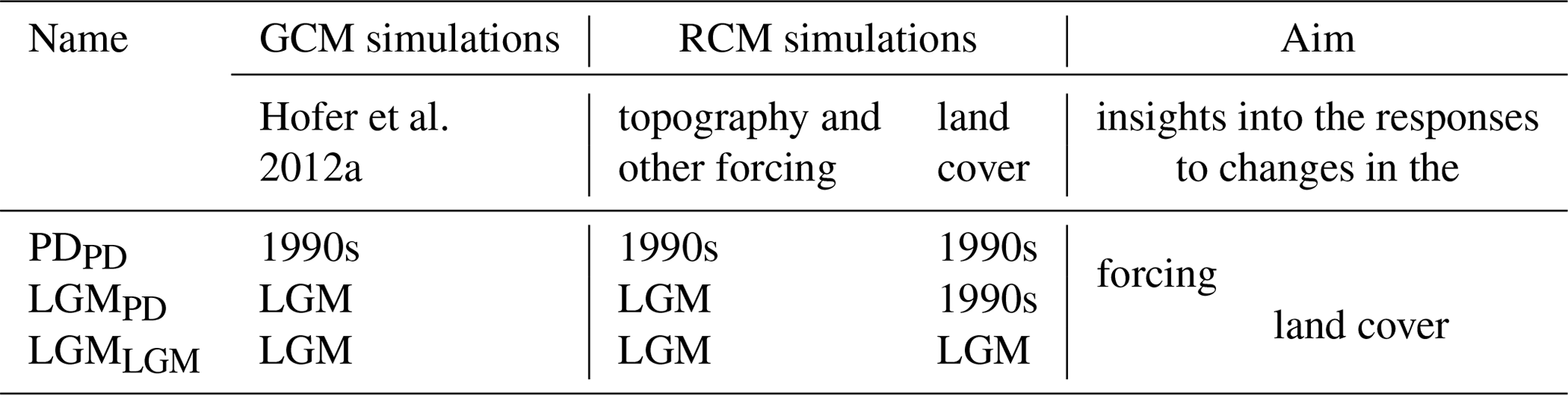
Comparing LGMPD with PDPD illustrates the atmospheric response to changes only in the atmospheric forcing, i.e. without changes in land cover. The comparison of LGMLGM and the LGMPD allows us to extract the influence of land cover on the atmosphere, i.e. without changes in atmospheric boundary conditions. These simulations are summarised in Table 1.
To assess the statistical significance of the responses, we use a bootstrapping technique (Wilks, 2011). This technique consists of randomly selecting elements from the original sample to generate a new sample. This is also called resampling whereby the number of elements remains unchanged. This procedure is repeated 1000 times. A new mean value is calculated from each resampling obtaining 1000 mean values that are used to build a probabilistic distribution function (PDF). We assess the significance of the mean value using a significance level of 0.01 for each PDF's tail. The bootstrapping technique is applied to the spatially averaged values using as elements the climatological mean values across Europe. We use one experiment to build the PDF on which we allocate the spatially averaged value of another experiment to assess the significance. Also, the bootstrapping technique is applied at each grid point using as elements the 30 yearly mean values. At each grid point, we obtain the PDF from one experiment on which we allocate the climatological mean value of another experiment to estimate the significance.
2.3 Dynamic global vegetation model: LPJ-LMfire
Land cover for the LGM is simulated by the LPJ-LMfire dynamic global vegetation model (Pfeiffer et al., 2013), which is an evolution of LPJ (Sitch et al., 2003). LPJ-LMfire is a processed-based, large-scale representation of vegetation dynamics and land–atmosphere water and carbon exchanges that simulates land cover patterns in response to climate, soils, and atmospheric CO2 concentrations (Prentice et al., 1992; Haxeltine and Prentice, 1996; Haxeltine et al., 1996; Kaplan, 2001; Kaplan et al., 2016). LPJ-LMfire simulates land cover in the form of the fractional coverage of nine plant functional types (PFTs), including tropical, temperate, and boreal trees and tropical and extratropical herbaceous vegetation (Sitch et al., 2003).
In each of our simulations, we drove LPJ-LMfire for 1020 years with the climate and forcing (greenhouse gases: CO2, N2O, and CH4) from the GCM and PD soil physical properties extrapolated out onto the continental shelves (Kaplan et al., 2016). Such a long simulation is not necessary to bring above-ground vegetation into quasi-equilibrium with climate, but it allows soil organic matter to equilibrate. Since the vegetation model is computationally inexpensive, we performed these millennium-long simulations so that they could be analysed for other purposes in the future.
2.4 Iterative asynchronous coupling design
To create the best possible estimate of European land cover for the LGM, we used an iterative asynchronous coupling design that combines CCSM4/WRF with the LPJ-LMfire model (resulting in the LGMLGM climate simulation). This coupling design consists of four steps: (i) the fully coupled CCSM4 provides atmospheric variables for the LGM to generate the first approximation of LGM land cover with LPJ-LMfire at a horizontal grid spacing of 1.25∘ × 0.9∘ (longitude × latitude); (ii) WRF is driven by the CCSM4 with LGM conditions and the first approximation of LGM land cover created in step (i) to generate the first downscaled atmospheric variables for the LGM at 54 and 18 km grid spacing; (iii) LPJ-LMfire is run with the downscaled LGM atmospheric variables (from step ii) to regenerate the LGM land cover at the RCM resolutions; and (iv) same as (ii) but WRF uses the land-surface boundary conditions simulated at 54 and 18 km. Steps (iii) and (iv) are carried out asynchronously over five additional iterations to achieve a quasi-equilibrium between the climate and land cover. Parts (i) and (ii) are regarded as the first iteration, and the iterations of (iii) and (iv) are regarded as the second to seventh iterations. The variables that are passed between the climate and vegetation models are summarised in Table 2. Vegetation cover fraction is defined as the fraction of ground covered by vegetation at each grid point, with values between 0 % and 100 %. Also, to classify vegetation cover fraction into the land cover categories required by WRF (according to NOAH-MP MODIS; Niu et al., 2011), we used a simple scheme based only on the cover fraction of the LPJ-LMfire PFTs. Note that we identified a problem with the land–sea mask and around glaciated areas which was fixed between the third and fourth iteration. To test whether the asynchronous coupling has reached a quasi-equilibrium state, we assess the statistical significance with a bootstrapping technique that is introduced at the end of Sect. 2.2.

The offline coupling design (Sect. 2.4) aims at generating a simulation of the LGM climate and land cover that is as realistic as possible. Thereby, it is important that the land cover and the climate is in quasi-equilibrium (Strandberg et al., 2011) in order to discard the source of uncertainty related to an unbalanced climate system. In this study, we determine the quasi-equilibrium in the land cover and the climate, first, through empirical observation and second, through a statistical test applied to a set of variables (see Sect. 2.4). To illustrate the differences between the iterations, we concentrate on climate and land cover changes over the ice-free land areas of Europe at LGM (in domain 2) using the following variables: the spatial climatology of total precipitation, temperature at 2 m, albedo, deep-soil temperature, cloud cover, leaf area index and vegetation cover fraction, and the number of grid points dominated by the following land cover categories: sparsely vegetated, tundra, forest, and shrublands (NOAH-MP MODIS categories, Niu et al., 2011). Land cover categories that are functionally similar are grouped together, e.g. wooded tundra, mixed tundra, and barren tundra are all combined into the category tundra. Some land cover categories are not considered in our analysis as they are poorly represented in both periods, e.g. savanna, grassland, and wetland, or are not relevant for the LGM, e.g. cropland and urban (Fig. 2a–b).

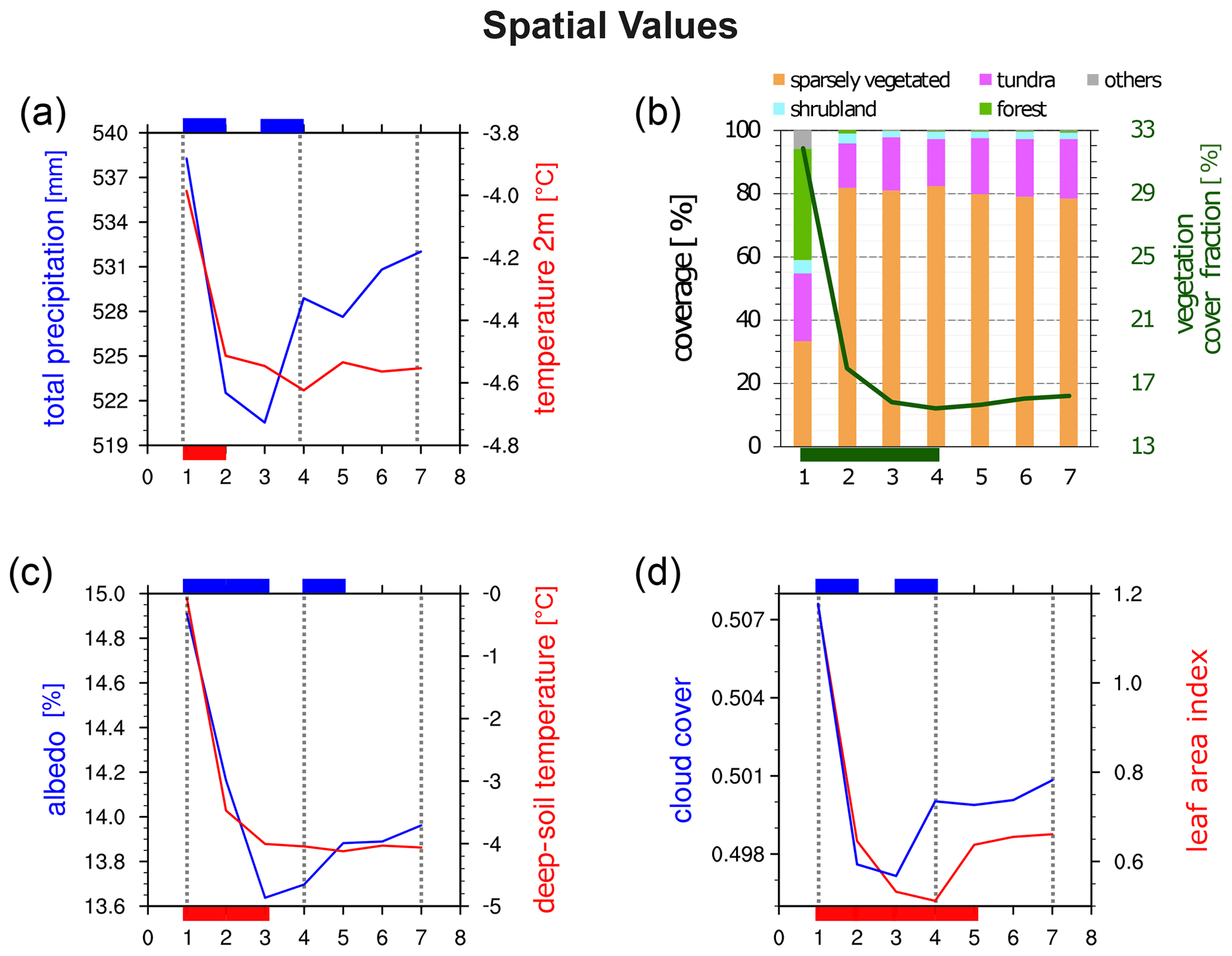
Figure 3Thirty-year spatial climatology of annual mean values throughout the iterations. Panel (a) represents total precipitation (blue line) and temperature at 2 m (red line) and (b) the percentage spatial fraction of bare (orange), tundra (pink), shrubland (sky blue), forest (light green), others (grey), and the spatial mean value of vegetation cover fraction (dark green line); (c) is the same as (a) but for albedo and deep-soil temperature, and (d) is the same as (a) but for cloud cover and leaf area index. The grey dotted lines in (a), (c), and (d) represent the first, fourth, and seventh iterations. Blue, red, and green boxes represent statistically significant differences between iterations at a 2 % significance level (using a two-tailed bootstrapping technique).
Results show that the most notable and statistically significant changes, from one iteration to the next, in the variables exchanged between land cover and atmosphere occur within the first four iterations (Fig. 3). Only albedo and leaf area index show significant changes also in the fifth iteration. The significance of the differences is assessed using a two-tailed bootstrapping technique with a significance level of 2 % (Sect. 2.2) and is marked in each panel of Fig. 3. Note that the significance for the land cover categories is not shown. The reason is that this significance can be summarised using the significance of the vegetation cover fraction. The variables level off from the fifth to the seventh iteration. In particular, we observe two sharp changes in all variables within the first five iterations. The first important change is found between the first and second iteration and is present in the atmospheric and land-surface variables. The reasoning is twofold: (i) there are significant changes in the land cover classes, e.g. forest fraction is reduced from 35 % to 2 %; (ii) the horizontal resolution of the land cover is increased from approximately 100 to 18 km (horizontal grid spacing of GCM and RCM, respectively). The higher spatial resolution of the RCM results in a better representation of the regional-to-local-scale processes and interactions with other components of the climate system compared to a GCM (Ludwig et al., 2019). The second change happens between the third and fourth iteration in precipitation and cloud cover (Fig. 3a and d) and between the fourth and fifth in albedo and leaf area index (Fig. 3c and d). Note that the improvements in the land–sea mask and around glaciated areas between the third and fourth iteration can partially explain the significantly sharp change in precipitation and cloud cover between the third and fourth iteration. We consider the significant changes from the fourth to the fifth iteration in albedo and leaf area index as a delayed effect of the variation in cloud cover and precipitation and thus an effect of the improvement.
Spatially averaged total precipitation significantly decreases in the second iteration (drop of 15 mm) and significantly increases in the fourth iteration (increase of 9 mm) with small and no significant changes thereafter (blue line in Fig. 3a). A significant decrease in the spatially averaged temperature at 2 m is observed in the second iteration (cooling of around 0.5 ∘C), which turns into small and insignificant fluctuations in the range of a 10th of a degree afterwards (red line in Fig. 3a). Albedo significantly decreases until the third iteration (change of around 1.3 %) and significantly increases in the fifth iteration with small and insignificant changes afterwards (blue line Fig. 3c). A significant cooling is also observed in the spatially averaged deep-soil temperature from the first to the third iteration (red line in Fig. 3c). Deep-soil temperature stabilises from the fourth to the seventh iteration. Similar to total precipitation, we observe that the spatially averaged cloud cover fraction significantly decreases in the second iteration (change of 0.009) and significantly increases in the fourth iteration (change of 0.003) with very small and insignificant variations afterwards (blue line in Fig. 3d). Leaf area index significantly fluctuates till the fifth iteration (maximum change of 0.5) with minimal and insignificant changes thereafter (red line Fig. 3d). Additionally, changes in vegetation cover fraction are observed in the first four iterations (32 %, 18 %, 16 %, and 15 %). In the following iterations, the changes remain rather small and insignificant (Fig. 3b). The land cover categories change mostly between the first and second iteration. The category sparsely vegetated is strongly increased in the second iteration and at the same time forest is strongly reduced (Fig. 3b). Thus, the quasi-equilibrium state is achieved after the fourth to fifth iteration.
In the following, we analyse the spatial patterns of climate and land cover between the iterations that represent the transient progression towards quasi-equilibrium (fourth minus first iteration) and the quasi-equilibrium state (seventh minus fourth iteration). We consider temperature at 2 m, total precipitation, and vegetation cover fraction as variables that summarise the coupled land–atmosphere response. Note that temperature, precipitation, and vegetation cover fraction are displayed using absolute differences (Fig. 4a–f).
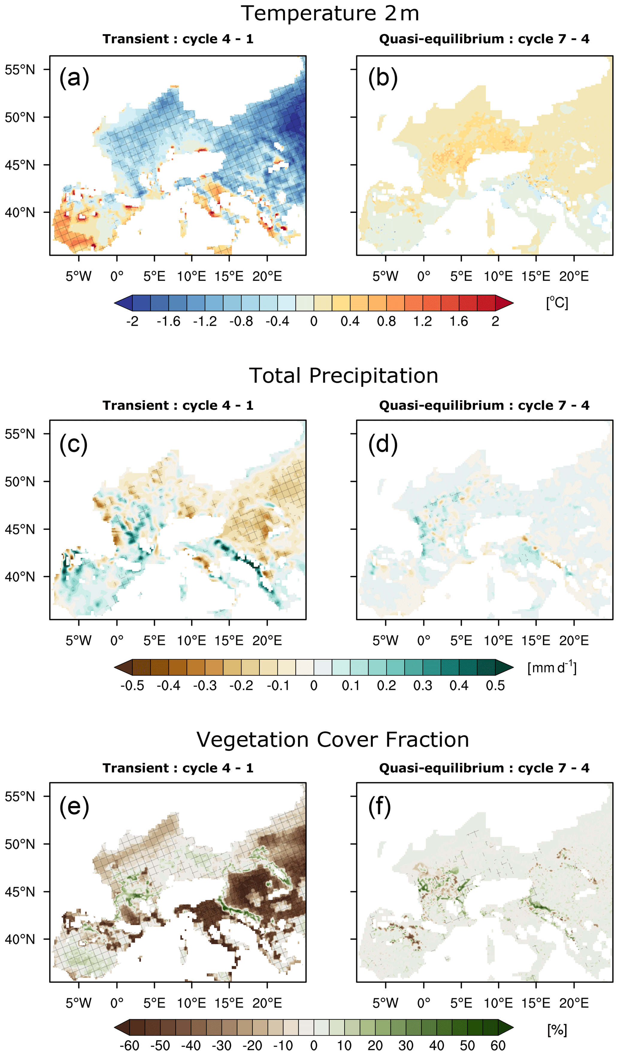
Figure 4Differences in 30-year mean values. Panel (a) represents the difference in temperature at 2 m between the first and fourth iteration (transient); (b) is the same as (a) but between the fourth and seventh iteration (quasi-equilibrium). Panels (c)–(d) and (e)–(f) are the same as (a)–(b) but for total precipitation and vegetation cover fraction, respectively. Masked out areas are in white. Crosshatched areas indicate statistically significant differences using a two-tailed bootstrapping technique with a 2 % significance level.
During the transient state (Fig. 4a, c, and e), the southwestern part of the Iberian Peninsula and some areas in Italy and Greece warm, but the rest of Europe experiences a cooling. In addition, precipitation reveals a wetting over the Iberian Peninsula, in parts of France, and in the Balkan Peninsula and a drying over eastern Europe, the north of the Alps, and some regions of France (Fig. 4c). The vegetation cover fraction shows a strong decrease during the transient state, particularly in the flat lands of eastern Europe (over 50 % reduction) and the Italian Peninsula, and an increase over the Iberian Peninsula (around 20 %) and northwest of the Alps (around 40 %; Fig. 4e). The vegetation response is related to changes in temperature and precipitation: many regions that experience a cooling are related to a reduction in vegetation. Drying and wetting are overall related to a reduction and an increase in vegetation cover, respectively. This is true except for a few areas in the north of the Alps and along the Mediterranean coast such as the eastern region of the Iberian Peninsula, southern Greece, and southern Italy. North of the Alps, the poor relation between precipitation and vegetation cover fraction could be explained by a lesser pronounced cooling. In the eastern part of the Iberian Peninsula and southern Greece, the reduction in vegetation seems to be related to an increase in temperature.
The changes between the seventh and fourth iterations, which illustrate the quasi-equilibrium state, are minimal for the three variables (Fig. 4b, d, and f). The remaining small differences are interpreted as a part of the internal climate variability and uncertainties predominantly caused by parameterisations in the models, e.g. cloud formation and microphysical processes (Casanueva et al., 2016; Rajczak and Schär, 2017; Shrestha et al., 2017; Knist et al., 2018; Yang et al., 2019).
To evaluate the LGMLGM climate simulation, we compared temperature and precipitation to pollen-based reconstructions. Wu et al. (2007) provided reconstructions of temperature and precipitation for the coldest and warmest months of the LGM at 14 sites in Europe. Thus, we considered 56 samples (14 sites × 2 variables × 2 months) in this comparison. For the model–proxy comparison, we use the nearest model grid point to the pollen site and consider the model and proxy reconstruction to agree when the model-based anomaly is within the 90 % confidence interval of the pollen-based anomaly (more details about the proxies in Wu et al., 2007). Note that the simulated temperature and precipitation are anomalies with respect to PDPD and that January and July values are selected to mimic the coldest and warmest months.
In general, cooler and drier anomalies are observed in the LGMLGM with especially pronounced cooling in January and drying in July (Fig. 5). This resembles the proxy evidence given by the pollen-based reconstruction of Wu et al. (2007). In January, we observe a positive precipitation anomaly of up to 7 mm d−1 over the Iberian Peninsula, northern Italy, and the Dinaric Alps (Fig. 5c). Overall, the LGMLGM climate agrees with the pollen-based paleoclimate reconstructions at three-quarters of the 56 samples.
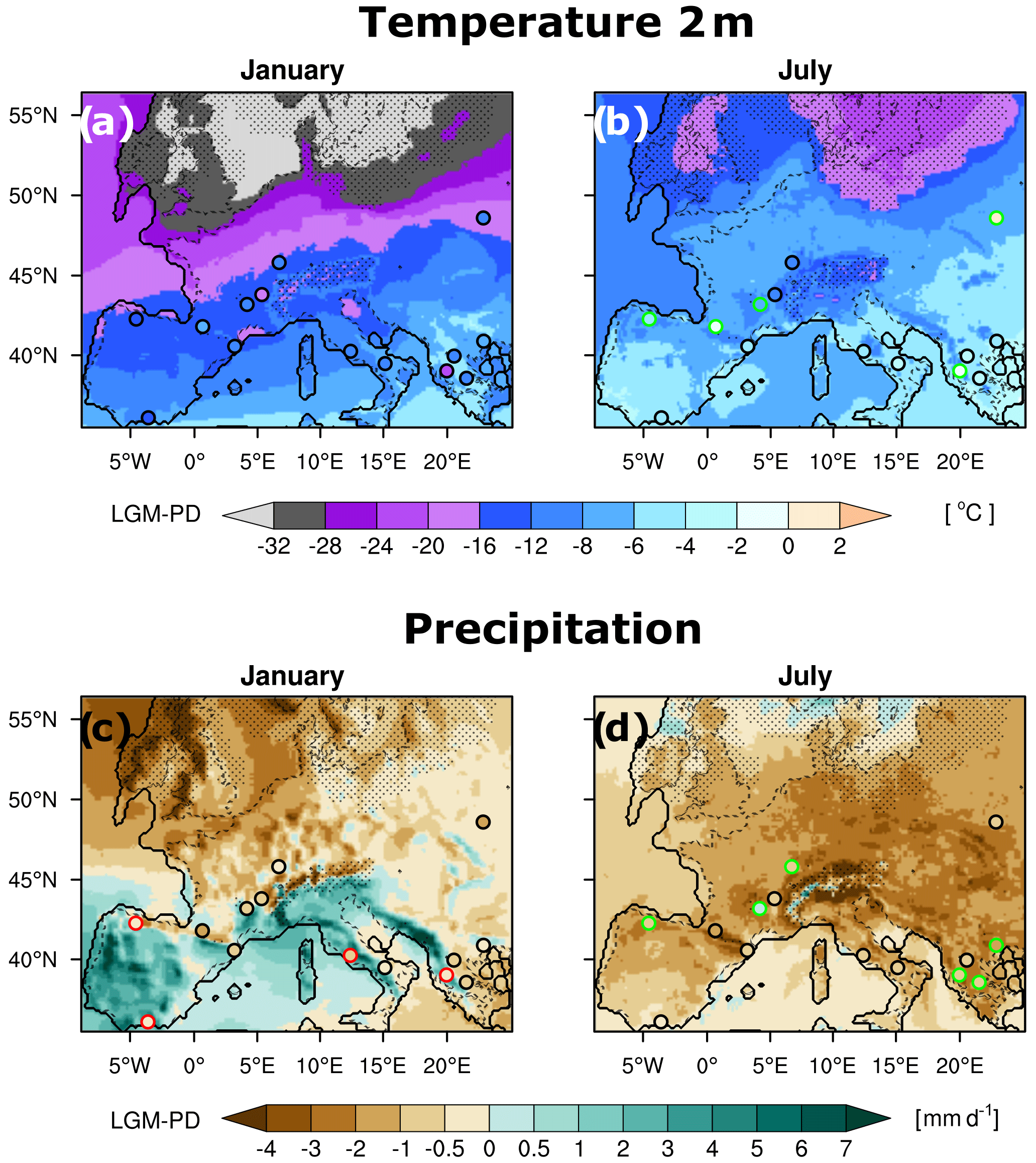
Figure 5Changes in temperature and precipitation patterns. Panel (a) represents the differences in 30-year mean temperature between LGM and PD (LGMLGM – PDPD) for January. Panel (b) is the same as (a) but for July. Panels (c) and (d) are the same as (a) and (b) but for precipitation differences. Circles represent proxy evidence: a red (green) border indicates that the simulated value is significantly above (below) the proxy value at the closest grid cell of the model (outside the 90 % confidence interval, Wu et al., 2007). The solid line represents the LGM coastline, the dashed line the PD coastline, and dots the area covered by glaciers.
Still, some samples, e.g. over the Iberian Peninsula, show considerable differences between the pollen-based and model-based climate anomalies, in line with similar findings mentioned in earlier studies (e.g. Beghin et al., 2016; Ludwig et al., 2016; Cleator et al., 2020). These differences can be associated with shortcomings within the GCM–RCM modelling chain and/or uncertainties in the proxy reconstructions (Bartlein et al., 2011; Ludwig et al., 2019; Cleator et al., 2020). Kageyama et al. (2006) suggested that terrestrial paleoclimate proxies may be more sensitive to climatic extremes than to the climatological mean state, which could partly explain the discrepancies between pollen-based reconstructions and the model simulations. One important model–proxy disagreement is the precipitation anomaly over the Iberian Peninsula in January. Based on evidence for the presence of certain tree species in the northwestern part of the Iberian Peninsula, Roucoux et al. (2005) suggested that the LGM was not necessarily the period of the most severe, i.e. cold and dry, climatic conditions everywhere. Roucoux et al. (2005) and Ludwig et al. (2018) also suggested that this region during LGM sensu stricto was warmer and wetter than the end of Marine Isotope Stage 3 (MIS3, ca. 23 ka; Voelker et al., 1997; Kreveld et al., 2000) and the start of the Heinrich event 1 (H1, ca. 19 ka; Sanchez Goñi and Harrison, 2010; Álvarez-Solas et al., 2011; Stanford et al., 2011). This could be an indication that model–proxy comparison fails because the proxies refer to 21±2 ka (Wu et al., 2007), i.e. either the end of MIS3 or the beginning of H1. Compared to the pre-industrial period, Beghin et al. (2016) found evidence in a model–proxy comparison that the interior and northwestern Iberian Peninsula experiences wetter conditions during the LGM. These wetter conditions can be explained by a southward shift in the North Atlantic storm track during the LGM compared to PD as suggested by many studies (e.g. Hofer et al., 2012a; Luetscher et al., 2015; Merz et al., 2015; Ludwig et al., 2016; Wang et al., 2018; Raible et al., 2020; Lofverstrom, 2020). Note further that we had only two pollen-based quantitative climate reconstructions from Iberia for the LGM; we therefore regard the model–proxy intercomparison in this region as equivocal.
To evaluate the LGMLGM and land cover simulation, we compare the simulated tree cover with pollen-based biome reconstructions from the BIOME6000 data product (Prentice and Jolly, 2000; Wu et al., 2007) and with a newer synthesis by Kaplan et al. (2016). For the purposes of this comparison, we define tree cover as the fraction of ground covered by trees at each grid point excluding herbaceous and grass, whose value varies between 0 % and 100 %.
The LGMLGM simulation generally shows low values for vegetation cover fraction (Fig. 2d), which reflects lower temperatures, reduced precipitation, and lower global atmospheric CO2 concentrations that were present at the LGM compared to the Holocene (Gerhart and Ward, 2010; Woillez et al., 2011; Chen et al., 2019; Lu et al., 2019). Our simulated LGMLGM land cover is generally in good agreement with the pollen-based biome reconstructions (Fig. 2b). We interpret the pollen reconstructions of steppe vegetation as sparsely vegetated in the WRF land cover categories (Niu et al., 2011). Using the nine nearest 18 km grid points surrounding each pollen site to compare the model results with pollen-based reconstructions of the land cover categories, we define good model–proxy agreement when at least one of the grid points matches the proxy reconstruction. For example, the dominant land cover category northwest of the Alps (47.73∘ N, 6.5∘ E) reconstructed from pollen (steppe) agrees with the surrounding simulated land cover (sparse vegetation). For the Carpathian Basin, an area with few proxy reconstructions, the modelled LGM land cover categories are tundra and grassland, which is in agreement with results found by Magyari et al. (2014a, b). Additionally, we simulate an extended area of tundra categories (i.e. wooded and mixed tundra) between the Alps and the Fennoscandian ice sheet which can be regarded as the northernmost ice-free area of Europe. Similarly, Kjellström et al. (2010) simulated an extended area of tundra-like vegetation in the northernmost ice-free areas of Europe for MIS3.
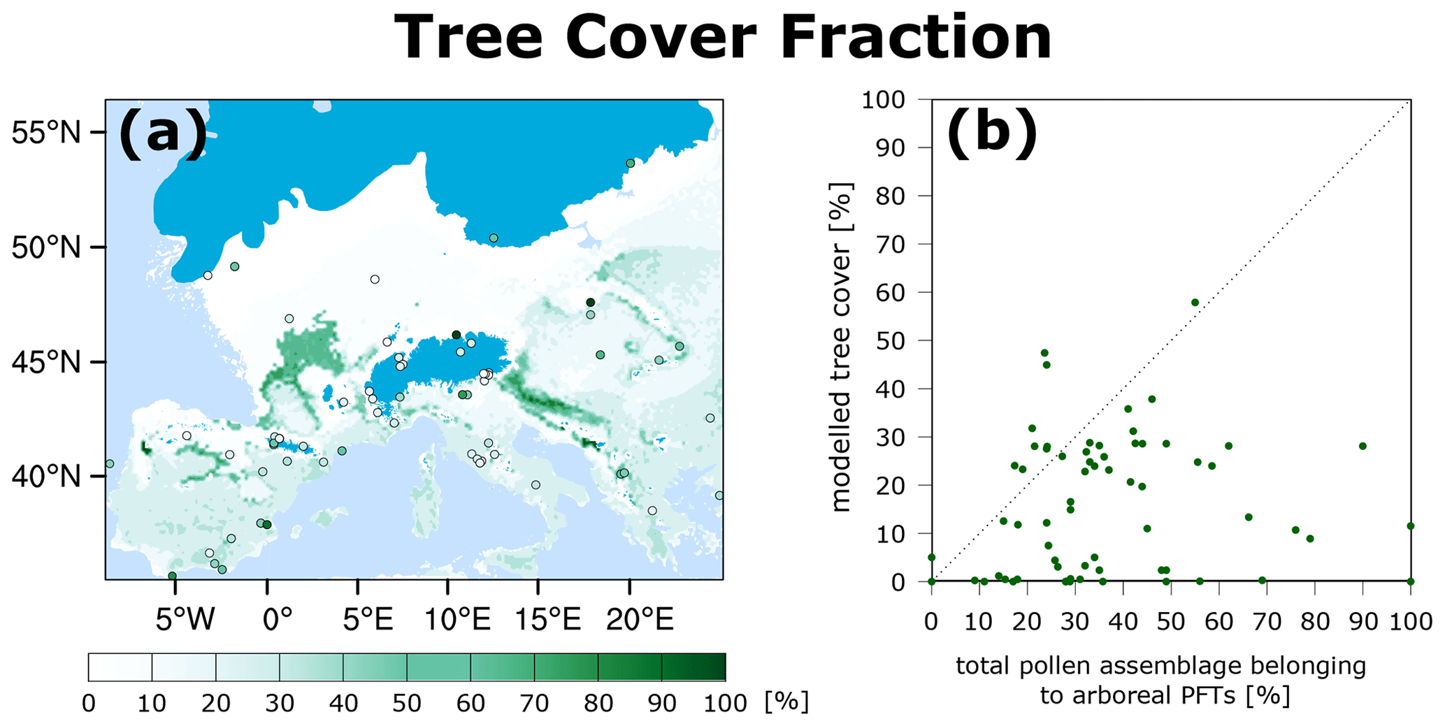
Figure 6Comparison between modelled and reconstructed tree cover. Panel (a) shows the LPJ-LMfire-simulated tree cover fraction from LGMLGM. Circles represent the 71 pollen samples securely dated to LGM from Kaplan et al. (2016). Panel (b) shows a scatter plot of reconstructed vs. modelled LGM tree cover.
We further compared tree cover fraction simulated by LPJ-LMfire with a reconstruction of relative landscape openness from 71 pollen sites across Europe containing samples securely dated to the LGM based on a compilation by Davis et al. (2015) and Kaplan et al. (2016). This compilation represents a substantial improvement in spatial coverage and dating precision compared to the 14 sites of BIOME6000 used by Wu et al. (2007). Comparison between modelled tree cover and relative landscape openness is shown in Fig. 6. Generally, LPJ-LMfire moderately underestimates tree cover compared with the pollen-based openness reconstructions. Modelled tree cover has a maximum value of about 60 %, while there are eight sites where the relative tree cover reconstruction is > 60 % and two samples with 100 % arboreal pollen percentage. As noted by Kaplan et al. (2016), these sites with very high reconstructed tree cover fraction should be treated with caution because they may represent locations with very little vegetation, e.g. at the edge of the Alpine ice sheet or at high-altitude in the Carpathian Mountains. In high mountain areas where we expect local vegetation to be very sparse if present at all, the pollen signal in sedimentary bodies may be dominated by the long-distance transport of tree pollen; this phenomenon is also observed in the analysis of pollen trapped in glacier ice (Brugger et al., 2019). At the bulk of the sites, LPJ-LMfire simulates 10 %–20 % lower tree cover than the relative tree cover inferred by the pollen. While this discrepancy is well within the uncertainty of both datasets and could be related to the calibration of arboreal pollen percentage with tree cover (Kaplan et al., 2016), it could also suggest that the modelled climate is too cold and/or too dry or that the LPJ-LMfire model is too sensitive to lower atmospheric CO2 concentrations.
We assess the atmospheric response to changes in the entire climate system, in external forcing, and in land cover, separately, to better understand the importance of the land surface for the LGM climate in Europe. LGMLGM is compared to PDPD to determine the atmospheric response to complete LGM conditions. Then, we investigate the atmospheric response to changes in orbital forcing by comparing LGMPD with PDPD. Finally, the differences between LGMLGM and LGMPD determine the atmospheric response to changes in land cover. Our assessment considers the land areas without snow/ice that are shared by both LGM and PD climate, i.e. we discard glaciated areas and land areas on the continental shelves that were exposed at the LGM. Temperature and precipitation are selected as the main indicators of the atmospheric response, and latent and sensible heat fluxes as secondary indicators. Note that we use a two-tailed bootstrapping technique with a significance level of 2 % to assess the significance of the differences (Sect. 2.2), which is illustrated by bold numbers in Table 3.
Table 3Assessment of the atmospheric response using 30 years of simulated precipitation and temperature data. First column indicates the simulations, second column the annual response, and the other columns the response in each season. Numbers in bold represent statistically significant differences using a two-tailed bootstrapping and a significance level of 2 %. Note that the assessment considers land areas without snow/ice that are shared by both LGM and PD climate and discards the continental shelves exposed at the LGM.
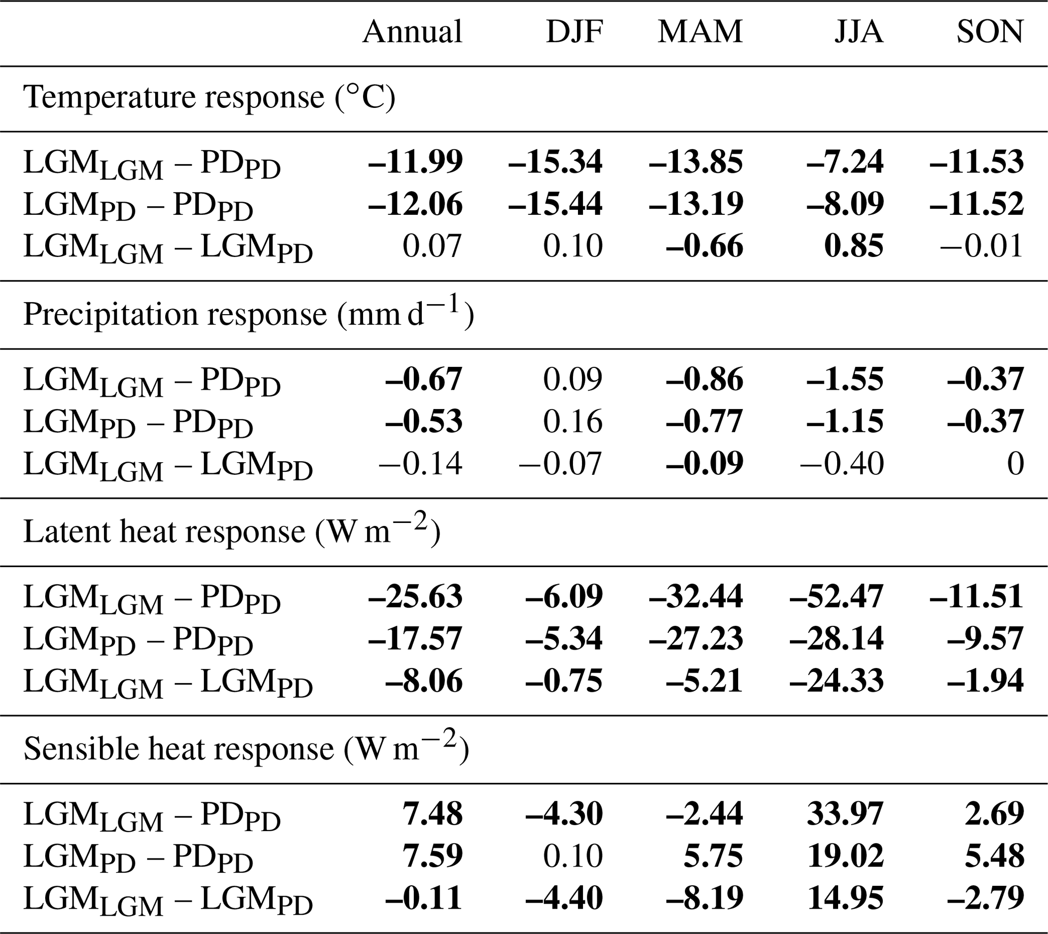
Comparing LGMLGM to PDPD shows a statistically significant cooling of −11.99 ∘C in the annual value (Table 3). This cooling is significantly enhanced to −15.34 ∘C in DJF (December–January–February), remains similar to the annual mean in MAM and SON (March–April–May and September–October–November), and significantly weakens to −7.24 ∘C in JJA (June–July–August; Table 3). This clearly illustrates a seasonality in the temperature response to complete LGM conditions (LGMLGM minus PDPD). Broccoli and Manabe (1987) mentioned that one reason for the seasonality in the temperature response can be the fluctuations in the horizontal thermal advection from glaciers and ice sheets to ice-free regions, predominantly in winter. Additionally, we find a statistically significant dryness in the annual value of around −0.67 mm d−1 when comparing LGMLGM to PDPD. A significant drying is evident in most months, in particular in summer months, where precipitation is reduced by −1.55 mm d−1. Only in the winter months do we observe a marginal increase in precipitation (Table 3). Cao et al. (2019) on the one hand attributed the overall decrease in precipitation to the strong anticyclonic circulations over the ice sheets during LGM compared to PD, especially to the low-level divergent cold air (Schaffernicht et al., 2020). On the other hand, Luetscher et al. (2015) and Lofverstrom (2020) found wetter conditions in southern parts of Europe in LGM wintertime, and they attributed them to atmospheric rivers and Rossby-wave breaking, respectively. This together with the LGM southward shift of the storm track (found by Hofer et al., 2012a; Luetscher et al., 2015; Ludwig et al., 2016; Wang et al., 2018; Raible et al., 2020) could then compensate for an expected dryness in wintertime (i.e. LGMLGM minus PDPD), which would not only affect the statistical significance in wintertime, but also lead to the seasonality in the precipitation response to complete LGM conditions. The comparison (LGMLGM minus PDPD) also shows a statistically significant decrease in latent heat flux in the annual value (−25.63 W m−2), which is true for most months and particularly strong for JJA (−52.47 W m−2). Moreover, we observe a statistically significant increase in sensible heat flux of 7.48 W m−2 (Table 3). This increase is strongest in JJA when it reaches an addition of 33.97 W m−2 and weakest in SON as we find a small but still significant increase of 2.69 W m−2. A statistically significant decrease in sensible heat flux of −4.30 and −2.44 W m−2 is simulated in DJF and MAM, respectively.
To further understand the atmospheric response, we investigate the role of the forcing (i.e. LGMPD – PDPD) and the land cover (i.e. LGMLGM – LGMPD), separately. The temperature response is clearly dominated by changes in the forcing. Changes in land cover can only slightly influence temperature by an additional cooling of 0.66 ∘C in MAM and a warming of 0.85 ∘C in JJA, both statistically significant (Table 3). Similarly, Jahn et al. (2005) found that the LGM-like vegetation cover produces colder temperatures (ca. −0.6 ∘C globally), especially in areas with the greatest decrease in tree cover. The precipitation anomalies are also dominated by changes in the forcing, whose values are statistically significant except in DJF, but changes in the land cover also contribute to a reduction in precipitation, especially in MAM (significant reduction of 0.09 mm d−1) and JJA (reduction of 0.40 mm d−1). The response of the latent heat flux is also dominated by changes in the forcing with statistically significant values. Changes in the land cover moderately influence the latent heat flux by an additional reduction of 8.06 W m−2 in the annual mean, while changes in land cover account for almost half of the reduction in the latent heat flux in JJA (−24.33 W m−2). Moreover, the response of the sensible heat flux is dominated by changes in the orbital forcing in the annual mean, JJA, and SON. Modifications in land cover only dominate DJF and MAM by an additional significant reduction of 4.40 and 8.19 W m−2, respectively. Still, changes in the land cover influence summer sensible heat by an additional increase of 14.95 W m−2.
The analysis so far demonstrates that the seasonality of the atmospheric response is overall driven by changes in the forcing but its intensity can be modulated by changes in the land cover, in particular in the latent heat flux in JJA and sensible heat flux in DJF, MAM, and JJA. A possible reason for the modulated intensity in the response may be a modification of the stability in the lowest levels of the atmosphere that is produced by the changes in the land cover. A cooling (warming) in the lower layer may lead to an inversion (unstable) zone that therefore weakens (enhances) precipitation processes. Another reason is that the differences in land cover lead to modifications in available moisture coming from the surface, i.e. evapotranspiration or latent heat. A reduction in latent heat is interpreted as reduced availability of surface moisture, which leads to a reduction in precipitation. Ludwig et al. (2017) suggested that including LGM-like vegetation in regional climate models causes changes in heat fluxes that lead to impacts on temperature and precipitation. Based on a similar coupling design, Strandberg et al. (2011) found that the impact of a different land cover on LGM climate simulations is small compared to the uncertainties in the proxy reconstructions. Even though this is also true in our study, our results and discussion suggest that modifications in land cover like deforestation could play an important role when other forcing agents marginally change, as is observed in some climate change scenarios such as RCP 2.6 and 4.5 (Strandberg and Kjellström, 2019; Davin et al., 2020; Jia et al., 2020).
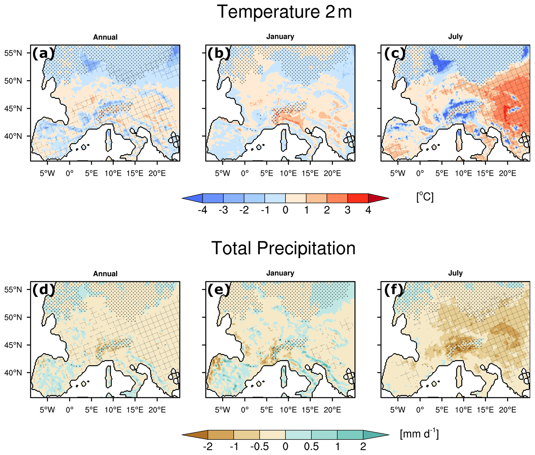
Figure 7Atmospheric response to changes in the land cover. Panel (a) shows differences in the annual mean temperature between LGMLGM – LGMPD. Panels (b) and (c) are the same as (a) but for January and July, respectively. Panels (d), (e), and (f) are the same as (a), (b), and (c) but for precipitation. The solid line represents the coastline during the LGM, stippled areas are covered by glaciers, and crosshatched areas indicate statistically significant differences using a two-tailed bootstrapping technique with a 2 % significance level.
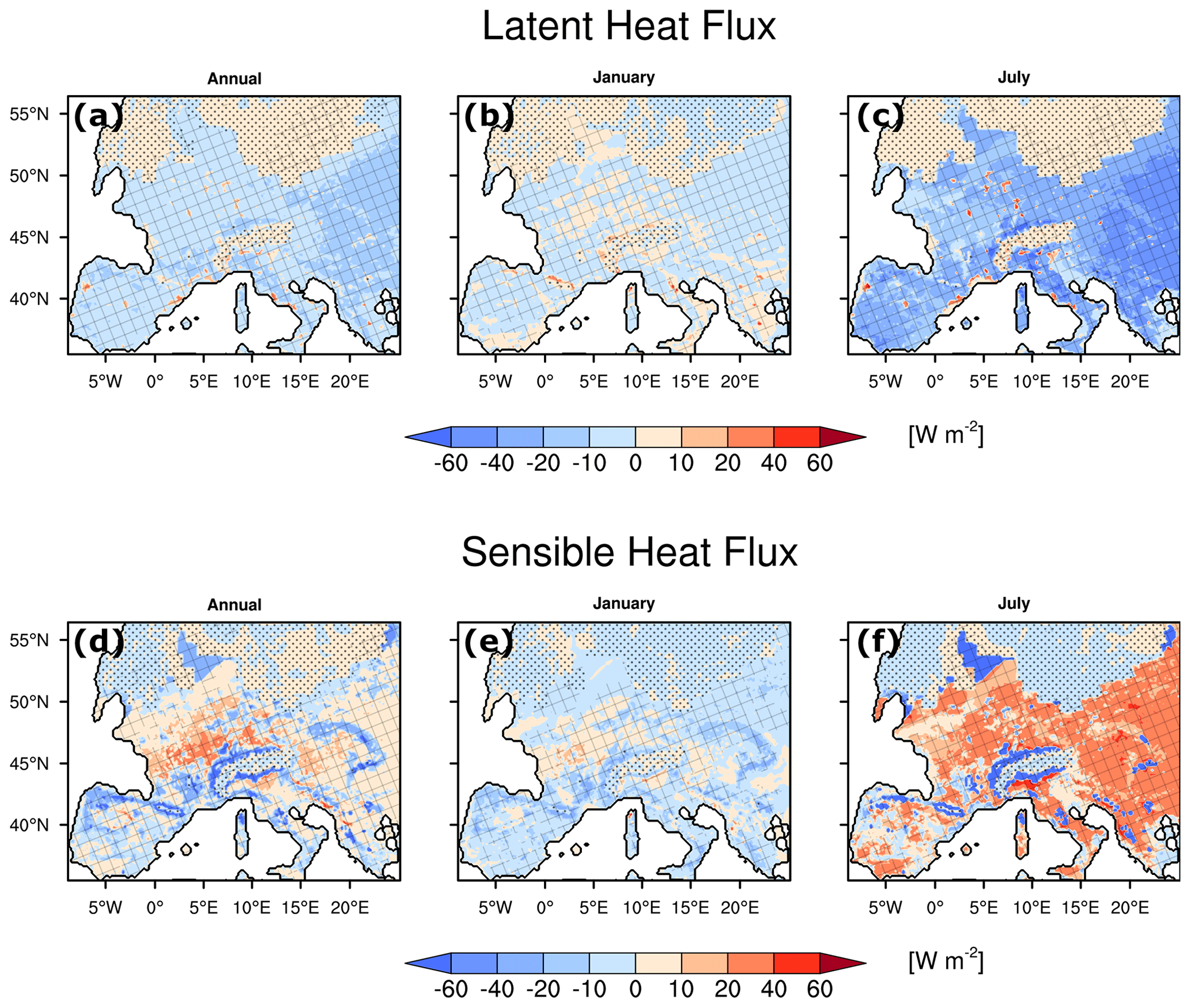
Figure 8Atmospheric response to changes in the land cover. Panel (a) represents differences in the annual mean latent heat flux between LGMLGM – LGMPD. Panels (b) and (c) are the same as (a) but for January and July, respectively. Panels (d), (e), and (f) are the same as (a), (b), and (c) but for sensible heat flux. The solid line represents the coastline during the LGM, stippled areas are covered by glaciers, and crosshatched areas indicate statistically significant differences using a two-tailed bootstrappping technique with a 2 % significance level.
To obtain a more detailed understanding of the atmospheric response to changes in land cover (LGMLGM – LGMPD), we further analyse the differences in the spatial patterns in January and July to be consistent with the evaluation done in Sect. 5. We focus on temperature at 2 m, precipitation and latent and sensible heat fluxes. We use a two-tailed bootstrapping technique with a significance level of 2 % to assess the significance of the differences at each grid point (Sect. 2.2), which is illustrated by crosshatched areas in Figs. 7 and 8.
The annual mean temperature shows a statistically significant cooling of around 2 ∘C in the vicinity of glaciers and in high-altitude regions; while a statistically significant warming is visible in lower-elevation areas including the southwestern part of the Iberian Peninsula, France, and the Carpathian Basin (Fig. 7a). A similar spatial pattern is observed for January and July temperatures: a significantly stronger warming is evident for the northern part of Italy in January (Fig. 7b), whereas the rest of the continent does not show significant changes. In July, the amplitude of the temperature anomaly becomes significantly stronger, especially where the positive temperature anomaly covers a large area, e.g. over eastern Europe (Fig. 7c). The precipitation response is moderate in the annual mean. A general and statistically significant decrease is observed over the rest of Europe. Changes in January precipitation are overall insignificant, except for some areas in eastern Europe where a significant dryness is observed. LGM land cover leads to a negative and statistically significant precipitation anomaly in July, which is especially strong around the Alps and in eastern Europe. The response of the latent heat flux is also moderate in the annual mean (Fig. 8a). We observe a general and statistically significant reduction, especially in eastern Europe. A similarly significant but weakened pattern is observed in January, which even shows a few small areas with an increase in latent heat flux (Fig. 8b). In July, a stronger reduction in the latent heat flux is observed with the largest reductions around the Alps and over eastern Europe (Fig. 8c). Note that some areas with strong increases in the latent heat flux (reddish) are associated with large PD urban areas. Moreover, the annual mean sensible heat flux shows a statistically significant reduction of about 30 W m−2 around mountainous areas, i.e. the Pyrenees, Alps, and Carpathian Mountains (Fig. 8d), while a statistically significant increase in sensible heat is visible in lower-elevation areas, especially over France and some areas in eastern Europe (Fig. 8d). In January, the pattern of the sensible heat flux is overall moderately reduced (still statistically significant, Fig. 8e). In July, we find an enhanced amplitude of the sensible heat flux with small changes in the spatial pattern with respect to the annual one: there is an additional statistically significant decrease in sensible heat flux of around 60 W m−2 around mountainous areas except for most of the Carpathian Mountains (Fig. 8f). A statistically significant increase in sensible heat flux dominates the rest of Europe, with values of up to 40 W m−2 in some areas over central and eastern Europe.
Even though changes in land cover have a small-to-moderate effect on the response of temperature, precipitation, and the latent and sensible heat fluxes (Table 3), their spatial pattern changes strongly across Europe (Figs. 7, 8). Important spatial changes are statistically significant over eastern Europe in July. Strandberg et al. (2011) and Kjellström et al. (2010), in similar coupling designs, compared glacial simulations using two land cover settings and found that the simulated regional climate patterns in parts of Europe are sensitive to feedbacks from large differences in vegetation. Particularly, Kjellström et al. (2010) found that glacial-like vegetation leads to warmer conditions over eastern Europe compared to modern vegetation. Strandberg et al. (2014) showed in their RCM experiments for the Holocene that summer temperature and precipitation are sensitive to changes in land cover in eastern Europe due to evapotranspiration (in our results as latent heat) feedbacks (see Fig. 8 in Strandberg et al., 2014). They found that a reduction in tree cover leads to warmer and drier summers in eastern Europe, which is similar to our finding as we observe that a reduction in vegetation cover fraction is associated with a warmer and drier July in the same region. This suggests that the land–atmosphere coupling strength may be stronger in eastern Europe compared to other parts of Europe, especially during summer.
In this study, we investigated the importance of land–atmosphere feedbacks for the climate of Europe during the Last Glacial Maximum. To this end, we performed a series of high-resolution asynchronously coupled atmosphere–vegetation model simulations. We simulated the European climate and vegetation using the WRF regional climate model and LPJ-LMfire vegetation model with a 54 and an 18 km horizontal grid spacing.
Results of the asynchronous coupling show that quasi-equilibrium between climate and land cover is reached after the fourth to fifth iteration. Between the first and fourth iterations, the climate becomes progressively wetter in southern Europe, while it becomes drier in eastern Europe. Once the coupled model system reaches quasi-equilibrium (from fourth to seventh iterations), we identified only marginal spatial differences that can be attributed to internal variability in the climate and vegetation models. The final iteration of the asynchronous coupling represents our best estimate of the atmospheric and land-surface conditions in Europe at the LGM. Consistent with many previous studies (e.g. Wu et al., 2007; Bartlein et al., 2011; Újvári et al., 2017; Cleator et al., 2020), we observe that the LGM climate of Europe was generally much colder and drier compared to PD. The LGMLGM land cover was characterised by tundra and sparse vegetation, although open forest parkland (transition from grass to forest during the LGM) may have been common in many parts of central Europe, which is supported by comparisons with pollen-based vegetation reconstructions.
Using two additional sensitivity simulations – PDPD and LGMPD – we quantified the direct effects of external forcing and land cover on the LGM climate. Comparing LGMLGM, i.e. the complete LGM conditions, to PDPD shows not only a general cooling and drying but also a seasonality in the atmospheric response. Comparing LGMPD to PDPD illustrates that the seasonality is mainly driven by changes in forcing. The comparison between LGMLGM to LGMPD shows that, even in Europe where we would generally expect a weak land–atmosphere coupling compared, e.g. to the monsoon tropics, the atmosphere is sensitive to changes in land cover. The land–atmosphere response also has a seasonality which differs across Europe with a stronger coupling strength in eastern Europe. These features can be partially explained by the variable spatial and temporal influence of vegetation cover (albedo) and heat fluxes (sensible and latent heat fluxes) to the lower troposphere. Our results show that dry conditions in the LGM are partially attributed to LGM land cover as a reduction in vegetation overall led to stronger dryness compared to PD land cover. This is particularly true for central and eastern Europe during summer.
An evaluation of the modelled LGMLGM climate should be performed with independent paleoclimate reconstructions from more sites than the 14 published points that are in the spatial domain of this study. Since the publication of Wu et al. (2007) and Bartlein et al. (2011), more than 70 well-dated pollen records from Europe that cover the LGM have become available (Kaplan et al., 2016). However, these data have not been transformed into paleoclimate reconstructions to date and such an effort would be beyond the scope of the current study. Additionally, as more paleoenvironmental reconstructions become available in the future, these simulations will be worthy of further evaluation and more detailed examination of specific areas. For instance, future work that improves pollen-based land cover reconstructions, e.g. using multi-proxy approaches that combine pollen data with presence–absence information from DNA (e.g. Alsos et al., 2020), will be very valuable for quantitative evaluation of model results using paleoenvironmental data. Although 18 km is a relatively high grid spacing for regional climate models, future studies will benefit from even more detailed climate simulations, particularly to better understand precipitation patterns in complex terrain such as Iberia, across the Mediterranean, and in the Carpathians. This is also true for studies on the local and regional paleobotany and archaeology of this important period in Europe's history.
WRF is a community model that can be downloaded from its web page (http://www2.mmm.ucar.edu/wrf/users/code_admin.php, Skamarock and Klemp, 2008). The source code of LPJ-LMfire can be downloaded from Github (https://github.com/ARVE-Research/LPJ-LMfire/tree/v1.3, last access: 4 November 2020; https://doi.org/10.5281/zenodo.1184589, Kaplan et al., 2018). The climate simulations (global: CCSM4 and regional: WRF) and land cover simulations (LPJ-LMfire) occupy several terabytes and thus are not freely available. Nevertheless, they can be accessed upon request to the contributing authors. Simple calculations carried out at a grid point level are performed with Climate Data Operator (CDO; https://doi.org/10.5281/zenodo.2558193, Schulzweida, 2019) and NCAR Command Language (NCL; https://doi.org/10.5065/D6WD3XH5, UCAR/NCAR/CISL/TDD, 2019). The figures are performed with NCL (UCAR/NCAR/CISL/TDD, 2019). The source code of the program to classify vegetation cover fraction into the WRF land cover categories is archived on Github (https://github.com/ARVE-Research/lpj2wrf; https://doi.org/10.5281/zenodo.4922199, Kaplan, 2021).
PV, JOK, and CCR contributed to the design of the experiments. PV carried out the climate simulations and wrote the first draft. JOK carried out the land cover simulations. PL provided the guidelines for introducing new land cover and LGM boundary conditions into WRF. MM provided support in the application of these guidelines. All authors contributed to the writing and scientific discussion.
The authors declare that they have no conflict of interest.
This work was supported by the Swiss National Science Foundation (SNF) within the project “Modelling the ice flow in the western Alps during the last glacial cycle”. Jed O. Kaplan is grateful for computing support from the School of Geography, University of Oxford. The simulations are performed on the supercomputing architecture of the Swiss National Supercomputing Centre (CSCS). Patrick Ludwig thanks the Helmholtz initiative REKLIM for funding. Martina Messmer is supported by the SNF Early Postdoc.Mobility programme. Data are locally stored on the oschgerstore provided by the Oeschger Center for Climate Change Research (OCCR). This study contributes to the PALEOLINK project as part of the PAGES 2k Network.
This research has been supported by the Schweizerischer Nationalfonds zur Förderung der Wissenschaftlichen Forschung (grant nos. 200021-162444 and P2BEP_181837).
This paper was edited by Qiuzhen Yin and reviewed by two anonymous referees.
Alsos, I. G., Sjögren, P., Brown, A. G., Gielly, L., Merkel, M. K. F., Paus, A., Lammers, Y., Edwards, M. E., Alm, T., Leng, M., Goslar, T., Langdon, C. T., Bakke, J., and van der Bilt, W. G. M.: Last Glacial Maximum environmental conditions at Andøya, northern Norway; evidence for a northern ice-edge ecological “hotspot”, Quaternary Sci. Rev., 239, 106364, https://doi.org/10.1016/j.quascirev.2020.106364, 2020. a
Álvarez-Solas, J., Montoya, M., Ritz, C., Ramstein, G., Charbit, S., Dumas, C., Nisancioglu, K., Dokken, T., and Ganopolski, A.: Heinrich event 1: an example of dynamical ice-sheet reaction to oceanic changes, Clim. Past, 7, 1297–1306, https://doi.org/10.5194/cp-7-1297-2011, 2011. a
Baena Preysler, J., Carrión Santafé, E., Torres Navas, C., and Vaquero Rodríguez, M.: Mousterian inside the upper Paleolithic? The last interval of El Esquilleu (Cantabria, Spain) sequence, Quatern. Int., 508, 153–163, https://doi.org/10.1016/j.quaint.2018.11.015, 2019. a
Bartlein, P. J., Harrison, S. P., Brewer, S., Connor, S., Davis, B. A. S., Gajewski, K., Guiot, J., Harrison-Prentice, T. I., Henderson, A., Peyron, O., Prentice, I. C., Scholze, M., Seppä, H., Shuman, B., Sugita, S., Thompson, R. S., Viau, A. E., Williams, J., and Wu, H.: Pollen-based continental climate reconstructions at 6 and 21 ka: a global synthesis, Clim. Dynam., 37, 775–802, https://doi.org/10.1007/s00382-010-0904-1, 2011. a, b, c, d, e
Beghin, P., Charbit, S., Kageyama, M., Combourieu-Nebout, N., Hatté, C., Dumas, C., and Peterschmitt, J.-Y.: What drives LGM precipitation over the western Mediterranean? A study focused on the Iberian Peninsula and northern Morocco, Clim. Dynam., 46, 2611–2631, https://doi.org/10.1007/s00382-015-2720-0, 2016. a, b, c, d
Berger, A.: Long-Term Variations of Daily Insolation and Quaternary Climatic Changes, J. Atmos. Sci., 35, 2362–2367, https://doi.org/10.1175/1520-0469(1978)035<2362:LTVODI>2.0.CO;2, 1978. a
Braconnot, P., Otto-Bliesner, B., Harrison, S., Joussaume, S., Peterchmitt, J.-Y., Abe-Ouchi, A., Crucifix, M., Driesschaert, E., Fichefet, Th., Hewitt, C. D., Kageyama, M., Kitoh, A., Laîné, A., Loutre, M.-F., Marti, O., Merkel, U., Ramstein, G., Valdes, P., Weber, S. L., Yu, Y., and Zhao, Y.: Results of PMIP2 coupled simulations of the Mid-Holocene and Last Glacial Maximum – Part 1: experiments and large-scale features, Clim. Past, 3, 261–277, https://doi.org/10.5194/cp-3-261-2007, 2007. a, b, c
Braconnot, P., Harrison, S. P., Kageyama, M., Bartlein, P. J., Masson-Delmotte, V., Abe-Ouchi, A., Otto-Bliesner, B., and Zhao, Y.: Evaluation of climate models using palaeoclimatic data, Nat. Clim. Change, 2, 417–424, https://doi.org/10.1038/nclimate1456, 2012. a
Broccoli, A. J. and Manabe, S.: The influence of continental ice, atmospheric CO2, and land albedo on the climate of the last glacial maximum, Clim. Dynam., 1, 87–99, https://doi.org/10.1007/BF01054478, 1987. a
Brugger, S. O., Gobet, E., Blunier, T., Morales-Molino, C., Lotter, A. F., Fischer, H., Schwikowski, M., and Tinner, W.: Palynological insights into global change impacts on Arctic vegetation, fire, and pollution recorded in Central Greenland ice, Holocene, 29, 1189–1197, https://doi.org/10.1177/0959683619838039, 2019. a
Burke, A., Levavasseur, G., James, P. M. A., Guiducci, D., Izquierdo, M. A., Bourgeon, L., Kageyama, M., Ramstein, G., and Vrac, M.: Exploring the impact of climate variability during the Last Glacial Maximum on the pattern of human occupation of Iberia, J. Hum. Evol., 73, 35–46, https://doi.org/10.1016/j.jhevol.2014.06.003, 2014. a
Cao, J., Wang, B., and Liu, J.: Attribution of the Last Glacial Maximum climate formation, Clim. Dynam., 53, 1661–1679, https://doi.org/10.1007/s00382-019-04711-6, 2019. a
Casanueva, A., Kotlarski, S., Herrera, S., Fernández, J., Gutiérrez, J. M., Boberg, F., Colette, A., Christensen, O. B., Goergen, K., Jacob, D., Keuler, K., Nikulin, G., Teichmann, C., and Vautard, R.: Daily precipitation statistics in a EURO-CORDEX RCM ensemble: Added value of raw and bias-corrected high-resolution simulations, Clim. Dynam., 47, 719–737, https://doi.org/10.1007/s00382-015-2865-x, 2016. a
Chen, W., Zhu, D., Ciais, P., Huang, C., Viovy, N., and Kageyama, M.: Response of vegetation cover to CO2 and climate changes between Last Glacial Maximum and pre-industrial period in a dynamic global vegetation model, Quaternary Sci. Rev., 218, 293–305, https://doi.org/10.1016/j.quascirev.2019.06.003, 2019. a
Clark, P. U., Dyke, A. S., Shakun, J. D., Carlson, A. E., Clark, J., Wohlfarth, B., Mitrovica, J. X., Hostetler, S. W., and McCabe, A. M.: The Last Glacial Maximum, Science, 325, 710–714, https://doi.org/10.1126/science.1172873, 2009. a, b
Cleator, S. F., Harrison, S. P., Nichols, N. K., Prentice, I. C., and Roulstone, I.: A new multivariable benchmark for Last Glacial Maximum climate simulations, Clim. Past, 16, 699–712, https://doi.org/10.5194/cp-16-699-2020, 2020. a, b, c, d, e
Crowley, T. J. and Baum, S. K.: Effect of vegetation on an ice-age climate model simulation, J. Geophys. Res.-Atmos., 102, 16463–16480, https://doi.org/10.1029/97JD00536, 1997. a
Davin, E. L., Rechid, D., Breil, M., Cardoso, R. M., Coppola, E., Hoffmann, P., Jach, L. L., Katragkou, E., de Noblet-Ducoudré, N., Radtke, K., Raffa, M., Soares, P. M. M., Sofiadis, G., Strada, S., Strandberg, G., Tölle, M. H., Warrach-Sagi, K., and Wulfmeyer, V.: Biogeophysical impacts of forestation in Europe: first results from the LUCAS (Land Use and Climate Across Scales) regional climate model intercomparison, Earth Syst. Dynam., 11, 183–200, https://doi.org/10.5194/esd-11-183-2020, 2020. a
Davis, B. A. S., Collins, P. M., and Kaplan, J. O.: The age and post-glacial development of the modern European vegetation: a plant functional approach based on pollen data, Veg. Hist. Archaeobot., 24, 303–317, https://doi.org/10.1007/s00334-014-0476-9, 2015. a
Demory, M.-E., Berthou, S., Fernández, J., Sørland, S. L., Brogli, R., Roberts, M. J., Beyerle, U., Seddon, J., Haarsma, R., Schär, C., Buonomo, E., Christensen, O. B., Ciarlo ̀, J. M., Fealy, R., Nikulin, G., Peano, D., Putrasahan, D., Roberts, C. D., Senan, R., Steger, C., Teichmann, C., and Vautard, R.: European daily precipitation according to EURO-CORDEX regional climate models (RCMs) and high-resolution global climate models (GCMs) from the High-Resolution Model Intercomparison Project (HighResMIP), Geosci. Model Dev., 13, 5485–5506, https://doi.org/10.5194/gmd-13-5485-2020, 2020. a
de Vernal, A., Rosell-Melé, A., Kucera, M., Hillaire-Marcel, C., Eynaud, F., Weinelt, M., Dokken, T., and Kageyama, M.: Comparing proxies for the reconstruction of LGM sea-surface conditions in the northern North Atlantic, Quaternary Sci. Rev., 25, 2820–2834, https://doi.org/10.1016/j.quascirev.2006.06.006, 2006. a
Di Luca, A., de Elía, R., and Laprise, R.: Potential for added value in precipitation simulated by high-resolution nested Regional Climate Models and observations, Clim. Dynam., 38, 1229–1247, https://doi.org/10.1007/s00382-011-1068-3, 2012. a
Ehlers, J., Gibbard, P., and Hughes, P.: Quaternary glaciations-extent and chronology: a closer look, vol. 15, Elsevier, Amsterdam, the Netherlands, 2011. a
Finlayson, C.: Neanderthals and modern humans: an ecological and evolutionary perspective, vol. 38, Cambridge University Press, Cambridge, UK, https://doi.org/10.1017/CBO9780511542374, 2004. a
Finlayson, C.: On the importance of coastal areas in the survival of Neanderthal populations during the Late Pleistocene, Quaternary Sci. Rev., 27, 2246–2252, https://doi.org/10.1016/j.quascirev.2008.08.033, 2008. a
Finlayson, C., Giles Pacheco, F., Rodríguez-Vidal, J., Fa, D. A., María Gutierrez López, J., Santiago Pérez, A., Finlayson, G., Allue, E., Baena Preysler, J., Cáceres, I., Carrión, J. S., Fernández Jalvo, Y., Gleed-Owen, C. P., Jimenez Espejo, F. J., López, P., Antonio López Sáez, J., Antonio Riquelme Cantal, J., Sánchez Marco, A., Giles Guzman, F., Brown, K., Fuentes, N., Valarino, C. A., Villalpando, A., Stringer, C. B., Martinez Ruiz, F., and Sakamoto, T.: Late survival of Neanderthals at the southernmost extreme of Europe, Nature, 443, 850–853, https://doi.org/10.1038/nature05195, 2006. a
Gent, P. R., Danabasoglu, G., Donner, L. J., Holland, M. M., Hunke, E. C., Jayne, S. R., Lawrence, D. M., Neale, R. B., Rasch, P. J., Vertenstein, M., Worley, P. H., Yang, Z.-L., and Zhang, M.: The Community Climate System Model Version 4, J. Climate, 24, 4973–4991, https://doi.org/10.1175/2011JCLI4083.1, 2011. a, b
Gerhart, L. M. and Ward, J. K.: Plant responses to low [CO2] of the past, New Phytol., 188, 674–695, https://doi.org/10.1111/j.1469-8137.2010.03441.x, 2010. a
Gómez-Navarro, J. J., Montávez, J. P., Jerez, S., Jiménez-Guerrero, P., Lorente-Plazas, R., González-Rouco, J. F., and Zorita, E.: A regional climate simulation over the Iberian Peninsula for the last millennium, Clim. Past, 7, 451–472, https://doi.org/10.5194/cp-7-451-2011, 2011. a
Gómez-Navarro, J. J., Montávez, J. P., Jiménez-Guerrero, P., Jerez, S., Lorente-Plazas, R., González-Rouco, J. F., and Zorita, E.: Internal and external variability in regional simulations of the Iberian Peninsula climate over the last millennium, Clim. Past, 8, 25–36, https://doi.org/10.5194/cp-8-25-2012, 2012. a, b
Gómez-Navarro, J. J., Montávez, J. P., Wagner, S., and Zorita, E.: A regional climate palaeosimulation for Europe in the period 1500–1990 – Part 1: Model validation, Clim. Past, 9, 1667–1682, https://doi.org/10.5194/cp-9-1667-2013, 2013. a, b
Gómez-Navarro, J. J., Bothe, O., Wagner, S., Zorita, E., Werner, J. P., Luterbacher, J., Raible, C. C., and Montávez, J. P.: A regional climate palaeosimulation for Europe in the period 1500–1990 – Part 2: Shortcomings and strengths of models and reconstructions, Clim. Past, 11, 1077–1095, https://doi.org/10.5194/cp-11-1077-2015, 2015. a
Harrison, S. P., Bartlein, P. J., Izumi, K., Li, G., Annan, J., Hargreaves, J., Braconnot, P., and Kageyama, M.: Evaluation of CMIP5 palaeo-simulations to improve climate projections, Nat. Clim. Change, 5, 735–743, https://doi.org/10.1038/nclimate2649, 2015. a
Haxeltine, A. and Prentice, I. C.: BIOME3: An equilibrium terrestrial biosphere model based on ecophysiological constraints, resource availability, and competition among plant functional types, Global Biogeochem. Cy., 10, 693–709, 1996. a
Haxeltine, A., Prentice, I. C., and Creswell, I. D.: A coupled carbon and water flux model to predict vegetation structure, J. Veg. Sci., 7, 651–666, https://doi.org/10.2307/3236377, 1996. a
Hofer, D., Raible, C. C., Dehnert, A., and Kuhlemann, J.: The impact of different glacial boundary conditions on atmospheric dynamics and precipitation in the North Atlantic region, Clim. Past, 8, 935–949, https://doi.org/10.5194/cp-8-935-2012, 2012a. a, b, c, d, e, f, g, h, i, j, k, l, m, n, o
Hofer, D., Raible, C. C., Merz, N., Dehnert, A., and Kuhlemann, J.: Simulated winter circulation types in the North Atlantic and European region for preindustrial and glacial conditions: Glacial circulation types, Geophys. Res. Lett., 39, L15805, https://doi.org/10.1029/2012GL052296, 2012b. a, b, c
Hunke, E. C. and Lipscomb, W. H.: CICE: the Los Alamos Sea Ice Model Documentation and Software User's Manual Version 4.1 LA-CC-06-012, Tech. rep., Los Alamos National Laboratory, Los Alamos, NM, USA, 2010. a
Iles, C. E., Vautard, R., Strachan, J., Joussaume, S., Eggen, B. R., and Hewitt, C. D.: The benefits of increasing resolution in global and regional climate simulations for European climate extremes, Geosci. Model Dev., 13, 5583–5607, https://doi.org/10.5194/gmd-13-5583-2020, 2020. a
Jahn, A., Claussen, M., Ganopolski, A., and Brovkin, V.: Quantifying the effect of vegetation dynamics on the climate of the Last Glacial Maximum, Clim. Past, 1, 1–7, https://doi.org/10.5194/cp-1-1-2005, 2005. a
Janská, V., Jiménez-Alfaro, B., Chytrý, M., Divíšek, J., Anenkhonov, O., Korolyuk, A., Lashchinskyi, N., and Culek, M.: Palaeodistribution modelling of European vegetation types at the Last Glacial Maximum using modern analogues from Siberia: Prospects and limitations, Quaternary Sci. Rev., 159, 103–115, https://doi.org/10.1016/j.quascirev.2017.01.011, 2017. a
Jia, G., Shevliakova, E., Artaxo, P., Noblet-Ducoudré, N. D., Houghton, R., House, J., Kitajima, K., Lennard, C., Popp, A., Sirin, A., Sukumar, R., and Verchot, L.: Land–climate interactions, in: Climate Change and Land: an IPCC special report on climate change, desertification, land degradation, sustainable land management, food security, and greenhouse gas fluxes in terrestrial ecosystems, edited by: Shukla, P. R., Skea, J., Calvo Buendia, E., Masson-Delmotte, V., Pörtner, H.-O., Roberts, D. C., Zhai, P., Slade, R., Connors, S., van Diemen, R., Ferrat, M., Haughey, E., Luz, S., Neogi, S., Pathak, M., Petzold, J., Portugal Pereira, J., Vyas, P., Huntley, E., Kissick, K., Belkacemi, M., and Malley, J., in press, 2019a. a
Jia, K., Ruan, Y., Yang, Y., and Zhang, C.: Assessing the Performance of CMIP5 Global Climate Models for Simulating Future Precipitation Change in the Tibetan Plateau, Water, 11, 1771, https://doi.org/10.3390/w11091771, 2019b. a
Jia, K.-H., Zhao, W., Maier, P. A., Hu, X.-G., Jin, Y., Zhou, S.-S., Jiao, S.-Q., El-Kassaby, Y. A., Wang, T., Wang, X.-R., and Mao, J.-F.: Landscape genomics predicts climate change-related genetic offset for the widespread Platycladus orientalis (Cupressaceae), Evol. Appl., 13, 665–676, 2020. a
Kageyama, M., Laîné, A., Abe-Ouchi, A., Braconnot, P., Cortijo, E., Crucifix, M., de Vernal, A., Guiot, J., Hewitt, C. D., Kitoh, A., Kucera, M., Marti, O., Ohgaito, R., Otto-Bliesner, B., Peltier, W. R., Rosell-Melé, A., Vettoretti, G., Weber, S. L., and Yu, Y.: Last Glacial Maximum temperatures over the North Atlantic, Europe and western Siberia: a comparison between PMIP models, MARGO sea–surface temperatures and pollen-based reconstructions, Quaternary Sci. Rev., 25, 2082–2102, https://doi.org/10.1016/j.quascirev.2006.02.010, 2006. a
Kageyama, M., Albani, S., Braconnot, P., Harrison, S. P., Hopcroft, P. O., Ivanovic, R. F., Lambert, F., Marti, O., Peltier, W. R., Peterschmitt, J.-Y., Roche, D. M., Tarasov, L., Zhang, X., Brady, E. C., Haywood, A. M., LeGrande, A. N., Lunt, D. J., Mahowald, N. M., Mikolajewicz, U., Nisancioglu, K. H., Otto-Bliesner, B. L., Renssen, H., Tomas, R. A., Zhang, Q., Abe-Ouchi, A., Bartlein, P. J., Cao, J., Li, Q., Lohmann, G., Ohgaito, R., Shi, X., Volodin, E., Yoshida, K., Zhang, X., and Zheng, W.: The PMIP4 contribution to CMIP6 – Part 4: Scientific objectives and experimental design of the PMIP4-CMIP6 Last Glacial Maximum experiments and PMIP4 sensitivity experiments, Geosci. Model Dev., 10, 4035–4055, https://doi.org/10.5194/gmd-10-4035-2017, 2017. a, b
Kageyama, M., Harrison, S. P., Kapsch, M.-L., Lofverstrom, M., Lora, J. M., Mikolajewicz, U., Sherriff-Tadano, S., Vadsaria, T., Abe-Ouchi, A., Bouttes, N., Chandan, D., Gregoire, L. J., Ivanovic, R. F., Izumi, K., LeGrande, A. N., Lhardy, F., Lohmann, G., Morozova, P. A., Ohgaito, R., Paul, A., Peltier, W. R., Poulsen, C. J., Quiquet, A., Roche, D. M., Shi, X., Tierney, J. E., Valdes, P. J., Volodin, E., and Zhu, J.: The PMIP4 Last Glacial Maximum experiments: preliminary results and comparison with the PMIP3 simulations, Clim. Past, 17, 1065–1089, https://doi.org/10.5194/cp-17-1065-2021, 2021. a, b
Kaplan, J. O.: Geophysical Applications of Vegetation Modeling, Doctoral dissertation, Lund University, Lund, Sweden, 2001. a
Kaplan, J. O.: ARVE-Research/lpj2wrf: first release (Version v1.0.0), Zenodo [code], https://doi.org/10.5281/zenodo.4922199, 2021. a
Kaplan, J. O., Pfeiffer, M., Kolen, J. C. A., and Davis, B. A. S.: Large scale anthropogenic reduction of forest cover in Last Glacial Maximum Europe, PLOS ONE, 11, e0166726, https://doi.org/10.1371/journal.pone.0166726, 2016. a, b, c, d, e, f, g, h
Kaplan, J. O., Pfeiffer, M., and Chaste, E.: ARVE-Research/LPJ-LMfire: LPJ-LMfire, Zenodo [code], https://doi.org/10.5281/zenodo.1184589, 2018. a
Kjellström, E., Brandefelt, J., Näslund, J.-O., Smith, B., Strandberg, G., Voelker, A. H. L., and Wohlfarth, B.: Simulated climate conditions in Europe during the Marine Isotope Stage 3 stadial, Boreas, 39, 436–456, https://doi.org/10.1111/j.1502-3885.2010.00143.x, 2010. a, b, c, d, e, f
Klein, K., Wegener, C., Schmidt, I., Rostami, M., Ludwig, P., Ulbrich, S., Richter, J., Weniger, G.-C., and Shao, Y.: Human existence potential in Europe during the Last Glacial Maximum, Quatern. Int., 581–582, 7–27, https://doi.org/10.1016/j.quaint.2020.07.046, 2021. a
Knist, S., Goergen, K., and Simmer, C.: Evaluation and projected changes of precipitation statistics in convection-permitting WRF climate simulations over Central Europe, Clim. Dynam., https://doi.org/10.1007/s00382-018-4147-x, 2018. a
Kreveld, S. v., Sarnthein, M., Erlenkeuser, H., Grootes, P., Jung, S., Nadeau, M. J., Pflaumann, U., and Voelker, A.: Potential links between surging ice sheets, circulation changes, and the Dansgaard-Oeschger Cycles in the Irminger Sea, 60–18 Kyr, Paleoceanography, 15, 425–442, https://doi.org/10.1029/1999PA000464, 2000. a
Landais, A., Masson-Delmotte, V., Capron, E., Langebroek, P. M., Bakker, P., Stone, E. J., Merz, N., Raible, C. C., Fischer, H., Orsi, A., Prié, F., Vinther, B., and Dahl-Jensen, D.: How warm was Greenland during the last interglacial period?, Clim. Past, 12, 1933–1948, https://doi.org/10.5194/cp-12-1933-2016, 2016. a
Lofverstrom, M.: A dynamic link between high-intensity precipitation events in southwestern North America and Europe at the Last Glacial Maximum, Earth Planet. Sc. Lett., 534, 116081, https://doi.org/10.1016/j.epsl.2020.116081, 2020. a, b
Lu, Z., Miller, P. A., Zhang, Q., Wårlind, D., Nieradzik, L., Sjolte, J., Li, Q., and Smith, B.: Vegetation pattern and terrestrial carbon variation in past warm and cold climates, Geophys. Res. Lett., 46, 8133–8143, https://doi.org/10.1029/2019GL083729, 2019. a
Ludwig, P., Schaffernicht, E. J., Shao, Y., and Pinto, J. G.: Regional atmospheric circulation over Europe during the Last Glacial Maximum and its links to precipitation, J. Geophys. Res.-Atmos., 121, 2130–2145, https://doi.org/10.1002/2015JD024444, 2016. a, b, c, d
Ludwig, P., Pinto, J. G., Raible, C. C., and Shao, Y.: Impacts of surface boundary conditions on regional climate model simulations of European climate during the Last Glacial Maximum, Geophys. Res. Lett., 44, 5086–5095, https://doi.org/10.1002/2017GL073622, 2017. a, b, c, d, e
Ludwig, P., Shao, Y., Kehl, M., and Weniger, G.-C.: The Last Glacial Maximum and Heinrich event I on the Iberian Peninsula: A regional climate modelling study for understanding human settlement patterns, Global Planet. Chang., 170, 34–47, https://doi.org/10.1016/j.gloplacha.2018.08.006, 2018. a
Ludwig, P., Gómez-Navarro, J. J., Pinto, J. G., Raible, C. C., Wagner, S., and Zorita, E.: Perspectives of regional paleoclimate modeling, Ann. NY Acad. Sci., 1436, 54–69, https://doi.org/10.1111/nyas.13865, 2019. a, b, c, d, e
Ludwig, P., Gavrilov, M. B., Markovic, S. B., Ujvari, G., and Lehmkuhl, F.: Simulated regional dust cycle in the Carpathian Basin and the Adriatic Sea region during the Last Glacial Maximum, Quatern. Int., 581–582, 114–127, https://doi.org/10.1016/j.quaint.2020.09.048, 2020. a
Luetscher, M., Boch, R., Sodemann, H., Spötl, C., Cheng, H., Edwards, R. L., Frisia, S., Hof, F., and Müller, W.: North Atlantic storm track changes during the Last Glacial Maximum recorded by Alpine speleothems, Nat. Commun., 6, 6344, https://doi.org/10.1038/ncomms7344, 2015. a, b, c
Magyari, E. K., Kuneš, P., Jakab, G., Sümegi, P., Pelánková, B., Schäbitz, F., Braun, M., and Chytrý, M.: Late Pleniglacial vegetation in eastern-central Europe: are there modern analogues in Siberia?, Quaternary Sci. Rev., 95, 60–79, https://doi.org/10.1016/j.quascirev.2014.04.020, 2014a. a
Magyari, E. K., Veres, D., Wennrich, V., Wagner, B., Braun, M., Jakab, G., Karátson, D., Pál, Z., Ferenczy, G., St-Onge, G., Rethemeyer, J., Francois, J. P., von Reumont, F., and Schäbitz, F.: Vegetation and environmental responses to climate forcing during the Last Glacial Maximum and deglaciation in the East Carpathians: attenuated response to maximum cooling and increased biomass burning, Quaternary Sci. Rev., 106, 278–298, https://doi.org/10.1016/j.quascirev.2014.09.015, 2014b. a
Maier, A., Lehmkuhl, F., Ludwig, P., Melles, M., Schmidt, I., Shao, Y., Zeeden, C., and Zimmermann, A.: Demographic estimates of hunter–gatherers during the Last Glacial Maximum in Europe against the background of palaeoenvironmental data, Quatern. Int., 425, 49–61, https://doi.org/10.1016/j.quaint.2016.04.009, 2016. a
Merz, N., Raible, C. C., Fischer, H., Varma, V., Prange, M., and Stocker, T. F.: Greenland accumulation and its connection to the large-scale atmospheric circulation in ERA-Interim and paleoclimate simulations, Clim. Past, 9, 2433–2450, https://doi.org/10.5194/cp-9-2433-2013, 2013. a
Merz, N., Born, A., Raible, C. C., Fischer, H., and Stocker, T. F.: Dependence of Eemian Greenland temperature reconstructions on the ice sheet topography, Clim. Past, 10, 1221–1238, https://doi.org/10.5194/cp-10-1221-2014, 2014a. a
Merz, N., Gfeller, G., Born, A., Raible, C. C., Stocker, T. F., and Fischer, H.: Influence of ice sheet topography on Greenland precipitation during the Eemian interglacial, J. Geophys. Res.-Atmos., 119, 10749–10768, https://doi.org/10.1002/2014JD021940, 2014b. a
Merz, N., Raible, C. C., and Woollings, T.: North Atlantic Eddy-Driven jet in interglacial and glacial winter climates, J. Climate, 28, 3977–3997, https://doi.org/10.1175/JCLI-D-14-00525.1, 2015. a, b, c, d, e
Merz, N., Born, A., Raible, C. C., and Stocker, T. F.: Warm Greenland during the last interglacial: the role of regional changes in sea ice cover, Clim. Past, 12, 2011–2031, https://doi.org/10.5194/cp-12-2011-2016, 2016. a
Mix, A. C., Bard, E., and Schneider, R.: Environmental processes of the ice age: land, oceans, glaciers (EPILOG), Quaternary Sci. Rev., 20, 627–657, https://doi.org/10.1016/S0277-3791(00)00145-1, 2001. a
Moreno, A., González-Sampériz, P., Morellón, M., Valero-Garcés, B. L., and Fletcher, W. J.: Northern Iberian abrupt climate change dynamics during the last glacial cycle: A view from lacustrine sediments, Quaternary Sci. Rev., 36, 139–153, https://doi.org/10.1016/j.quascirev.2010.06.031, 2012. a
Neale, R. B., Richter, J. H., Conley, A. J., Park, S., Lauritzen, P. H., Gettelman, A., Rasch, P. J., and Vavrus, J.: Description of the NCAR community atmosphere model (CAM4), National Center for Atmospheric Research Tech. Rep. NCAR/TN+ STR, available at: http://www.cesm.ucar.edu/models/ccsm4.0/cam/docs/description/cam4_desc.pdf (last access: 9 June 2021), 2010. a
Niu, G.-Y., Yang, Z.-L., Mitchell, K. E., Chen, F., Ek, M. B., Barlage, M., Kumar, A., Manning, K., Niyogi, D., Rosero, E., Tewari, M., and Xia, Y.: The community Noah land surface model with multiparameterization options (Noah-MP): 1. Model description and evaluation with local-scale measurements, J. Geophys. Res.-Atmos., 116, D12109, https://doi.org/10.1029/2010JD015139, 2011. a, b, c
Noblet, N. I. d., Prentice, I. C., Joussaume, S., Texier, D., Botta, A., and Haxeltine, A.: Possible role of atmosphere-biosphere interactions in triggering the Last Glaciation, Geophys. Res. Lett., 23, 3191–3194, https://doi.org/10.1029/96GL03004, 1996. a
Oleson, W., Lawrence, M., Bonan, B., Flanner, G., Kluzek, E., Lawrence, J., Levis, S., Swenson, C., Thornton, E., Dai, A., Decker, M., Dickinson, R., Feddema, J., Heald, L., Hoffman, F., Lamarque, J.-F., Mahowald, N., Niu, G.-Y., Qian, T., Randerson, J., Running, S., Sakaguchi, K., Slater, A., Stockli, R., Wang, A., Yang, Z.-L., Zeng, X., and Zeng, X.: Technical description of version 4.0 of the community land model (CLM), NCAR Technical Note NCAR/TN-478+STR, National Center for Atmospheric Research, Boulder, CO, USA, available at: http://www.cesm.ucar.edu/models/cesm1.0/clm/CLM4_Tech_Note.pdf (last access: 9 June 2021), 2010. a
Peltier, W.: Global glacial isostasy and the surface of the ice-age Earth: The ICE-5G (VM2) model and grace, Annu. Rev. Earth Pl. Sc., 32, 111–149, https://doi.org/10.1146/annurev.earth.32.082503.144359, 2004. a
Pfeiffer, M., Spessa, A., and Kaplan, J. O.: A model for global biomass burning in preindustrial time: LPJ-LMfire (v1.0), Geosci. Model Dev., 6, 643–685, https://doi.org/10.5194/gmd-6-643-2013, 2013. a, b
Prein, A. F., Holland, G. J., Rasmussen, R. M., Done, J., Ikeda, K., Clark, M. P., and Liu, C. H.: Importance of Regional Climate Model Grid Spacing for the Simulation of Heavy Precipitation in the Colorado Headwaters, J. Climate, 26, 4848–4857, https://doi.org/10.1175/JCLI-D-12-00727.1, 2013. a
Prentice, I. C. and Jolly, D.: Mid-Holocene and glacial-maximum vegetation geography of the northern continents and Africa, J. Biogeogr., 27, 507–519, https://doi.org/10.1046/j.1365-2699.2000.00425.x, 2000. a
Prentice, I. C., Cramer, W., Harrison, S. P., Leemans, R., Monserud, R. A., and Solomon, A. M.: Special Paper: A Global Biome Model Based on Plant Physiology and Dominance, Soil Properties and Climate, J. Biogeogr., 19, 117–134, https://doi.org/10.2307/2845499, 1992. a
Raible, C. C., Pinto, J. G., Ludwig, P., and Messmer, M.: A review of past changes in extratropical cyclones in the northern hemisphere and what can be learned for the future, WIRES Clim. Change, 12, e680, https://doi.org/10.1002/wcc.680, 2020. a, b, c, d
Rajczak, J. and Schär, C.: Projections of future precipitation extremes over Europe: A multimodel assessment of climate simulations, J. Geophys. Res.-Atmos., 122, 10773–10800, https://doi.org/10.1002/2017JD027176, 2017. a
Rauscher, S. A., Coppola, E., Piani, C., and Giorgi, F.: Resolution effects on regional climate model simulations of seasonal precipitation over Europe, Clim. Dynam., 35, 685–711, https://doi.org/10.1007/s00382-009-0607-7, 2010. a
Roucoux, K. H., de Abreu, L., Shackleton, N. J., and Tzedakis, P. C.: The response of NW Iberian vegetation to North Atlantic climate oscillations during the last 65 kyr, Quaternary Sci. Rev., 24, 1637–1653, https://doi.org/10.1016/j.quascirev.2004.08.022, 2005. a, b
Sanchez Goñi, M. F. and Harrison, S. P.: Millennial-scale climate variability and vegetation changes during the Last Glacial: Concepts and terminology, Quaternary Sci. Rev., 29, 2823–2827, https://doi.org/10.1016/j.quascirev.2009.11.014, 2010. a
Schaffernicht, E. J., Ludwig, P., and Shao, Y.: Linkage between dust cycle and loess of the Last Glacial Maximum in Europe, Atmos. Chem. Phys., 20, 4969–4986, https://doi.org/10.5194/acp-20-4969-2020, 2020. a
Schulzweida, U.: CDO User Guide (Version 1.9.6), Zenodo, https://doi.org/10.5281/zenodo.2558193, 2019. a
Seguinot, J., Ivy-Ochs, S., Jouvet, G., Huss, M., Funk, M., and Preusser, F.: Modelling last glacial cycle ice dynamics in the Alps, The Cryosphere, 12, 3265–3285, https://doi.org/10.5194/tc-12-3265-2018, 2018. a
Shrestha, R. K., Connolly, P. J., and Gallagher, M. W.: Sensitivity of WRF Cloud Microphysics to Simulations of a Convective Storm Over the Nepal Himalayas, The Open Atmospheric Science Journal, 11, 29–43, https://doi.org/10.2174/1874282301711010029, 2017. a
Sitch, S., Smith, B., Prentice, I. C., Arneth, A., Bondeau, A., Cramer, W., Kaplan, J. O., Levis, S., Lucht, W., Sykes, M. T., Thonicke, K., and Venevsky, S.: Evaluation of ecosystem dynamics, plant geography and terrestrial carbon cycling in the LPJ dynamic global vegetation model, Glob. Change Biol., 9, 161–185, https://doi.org/10.1046/j.1365-2486.2003.00569.x, 2003. a, b
Skamarock, W. C. and Klemp, J. B.: A time-split nonhydrostatic atmospheric model for weather research and forecasting applications, J. Comput. Phys., 227, 3465–3485, https://doi.org/10.1016/j.jcp.2007.01.037, 2008 (data available at: http://www2.mmm.ucar.edu/wrf/users/code_admin.php, last access: 12 October 2020). a, b, c, d
Skamarock, W. C., Klemp, J. B., Dudhia, J., Gill, O., Barker, D., Duda, G., Huang, X.-y., Wang, W., and Powers, G.: A description of the advanced research WRF version 3, (No. NCAR/TN-475+STR), University Corporation for Atmospheric Research, https://doi.org/10.5065/D68S4MVH, 2008. a, b
Stanford, J. D., Rohling, E. J., Bacon, S., Roberts, A. P., Grousset, F. E., and Bolshaw, M.: A new concept for the paleoceanographic evolution of Heinrich event 1 in the North Atlantic, Quaternary Sci. Rev., 30, 1047–1066, https://doi.org/10.1016/j.quascirev.2011.02.003, 2011. a
Strandberg, G. and Kjellström, E.: Climate impacts from afforestation and deforestation in Europe, Earth Interact., 23, 1–27, https://doi.org/10.1175/EI-D-17-0033.1, 2019. a
Strandberg, G., Brandefelt, J., Kjellstro M., E., and Smith, B.: High-resolution regional simulation of Last Glacial Maximum climate in Europe, Tellus A, 63, 107–125, https://doi.org/10.1111/j.1600-0870.2010.00485.x, 2011. a, b, c, d, e, f
Strandberg, G., Kjellström, E., Poska, A., Wagner, S., Gaillard, M.-J., Trondman, A.-K., Mauri, A., Davis, B. A. S., Kaplan, J. O., Birks, H. J. B., Bjune, A. E., Fyfe, R., Giesecke, T., Kalnina, L., Kangur, M., van der Knaap, W. O., Kokfelt, U., Kuneš, P., Latałowa, M., Marquer, L., Mazier, F., Nielsen, A. B., Smith, B., Seppä, H., and Sugita, S.: Regional climate model simulations for Europe at 6 and 0.2 k BP: sensitivity to changes in anthropogenic deforestation, Clim. Past, 10, 661–680, https://doi.org/10.5194/cp-10-661-2014, 2014. a, b, c
Texier, D., de Noblet, N., Harrison, S. P., Haxeltine, A., Jolly, D., Joussaume, S., Laarif, F., Prentice, I. C., and Tarasov, P.: Quantifying the role of biosphere-atmosphere feedbacks in climate change: coupled model simulations for 6000 years BP and comparison with palaeodata for northern Eurasia and northern Africa, Clim. Dynam., 13, 865–881, https://doi.org/10.1007/s003820050202, 1997. a
UCAR/NCAR/CISL/TDD: The NCAR Command Language (Version 6.6.2) [Software], https://doi.org/10.5065/D6WD3XH5, 2019. a, b
Újvári, G., Stevens, T., Molnár, M., Demény, A., Lambert, F., Varga, G., Jull, A. J. T., Páll-Gergely, B., Buylaert, J.-P., and Kovács, J.: Coupled European and Greenland last glacial dust activity driven by North Atlantic climate, P. Natl. Acad. Sci. USA, 114, E10632–E10638, https://doi.org/10.1073/pnas.1712651114, 2017. a
Van Meerbeeck, C. J., Renssen, H., and Roche, D. M.: How did Marine Isotope Stage 3 and Last Glacial Maximum climates differ? – Perspectives from equilibrium simulations, Clim. Past, 5, 33–51, https://doi.org/10.5194/cp-5-33-2009, 2009. a
Vegas, J., Ruiz-Zapata, B., Ortiz, J. E., Galán, L., Torres, T., García-Cortés, Á., Gil-García, M. J., Pérez-González, A., and Gallardo-Millán, J. L.: Identification of arid phases during the last 50 cal. ka BP from the Fuentillejo maar-lacustrine record (Campo de Calatrava Volcanic Field, Spain), J. Quaternary Sci., 25, 1051–1062, https://doi.org/10.1002/jqs.1262, 2010. a
Velasquez, P., Messmer, M., and Raible, C. C.: A new bias-correction method for precipitation over complex terrain suitable for different climate states: a case study using WRF (version 3.8.1), Geosci. Model Dev., 13, 5007–5027, https://doi.org/10.5194/gmd-13-5007-2020, 2020. a
Voelker, A. H. L., Sarnthein, M., Grootes, P. M., Erlenkeuser, H., Laj, C., Mazaud, A., Nadeau, M.-J., and Schleicher, M.: Correlation of Marine 14C Ages from the Nordic Seas with the GISP2 Isotope Record: Implications for 14C Calibration Beyond 25 ka BP, Radiocarbon, 40, 517–534, https://doi.org/10.1017/S0033822200018397, 1997. a
Walsh, J. E., Chapman, W. L., Romanovsky, V., Christensen, J. H., and Stendel, M.: Global Climate Model Performance over Alaska and Greenland, J. Climate, 21, 6156–6174, https://doi.org/10.1175/2008JCLI2163.1, 2008. a
Wang, N., Jiang, D., and Lang, X.: Northern Westerlies during the Last Glacial Maximum: Results from CMIP5 Simulations, J. Climate, 31, 1135–1153, https://doi.org/10.1175/JCLI-D-17-0314.1, 2018. a, b
Wilks, D. S.: Statistical methods in the atmospheric sciences, Academic Press, Burlington, MA, USA, San Diego, California, USA, London, UK, google-Books-ID: IJuCVtQ0ySIC, 2011. a
Woillez, M.-N., Kageyama, M., Krinner, G., de Noblet-Ducoudré, N., Viovy, N., and Mancip, M.: Impact of CO2 and climate on the Last Glacial Maximum vegetation: results from the ORCHIDEE/IPSL models, Clim. Past, 7, 557–577, https://doi.org/10.5194/cp-7-557-2011, 2011. a
Wu, H., Guiot, J., Brewer, S., and Guo, Z.: Climatic changes in Eurasia and Africa at the last glacial maximum and mid-Holocene: reconstruction from pollen data using inverse vegetation modelling, Clim. Dynam., 29, 211–229, https://doi.org/10.1007/s00382-007-0231-3, 2007. a, b, c, d, e, f, g, h, i, j, k, l, m, n
Yang, Q., Dai, Q., Han, D., Chen, Y., and Zhang, S.: Sensitivity analysis of raindrop size distribution parameterizations in WRF rainfall simulation, Atmos. Res., 228, 1–13, https://doi.org/10.1016/j.atmosres.2019.05.019, 2019. a
Yokoyama, Y., Lambeck, K., De Deckker, P., Johnston, P., and Fifield, L. K.: Timing of the Last Glacial Maximum from observed sea-level minima, Nature, 406, 713–716, https://doi.org/10.1038/35021035, 2000. a
- Abstract
- Introduction
- Models and methods
- Results of the iterative asynchronous coupling
- Comparison and discussion of the modelled and reconstructed climate
- Comparison and discussion of the modelled and reconstructed land cover
- Influence of external forcing and land cover on climate
- Conclusions
- Code and data availability
- Author contributions
- Competing interests
- Acknowledgements
- Financial support
- Review statement
- References