A data–model approach to interpreting speleothem oxygen isotope records from monsoon regions

Reconstruction of past changes in monsoon climate from speleothem oxygen isotope (δ¹⁸O) records is complex because δ¹⁸O signals can be influenced by multiple factors including changes in precipitation, precipitation recycling over land, temperature at the moisture source, and changes in the moisture source region and transport pathway. Here, we analyse >150 speleothem records of the Speleothem Isotopes Synthesis and AnaLysis (SISAL) database to produce composite regional trends in δ¹⁸O in monsoon regions; compositing minimises the influence of site-specific karst and cave processes that can influence individual site records. We compare speleothem δ¹⁸O observations with isotope-enabled climate model simulations to investigate the specific climatic factors causing these regional trends. We focus on differences in δ¹⁸O signals between the mid-Holocene, the peak of the Last Interglacial (Marine Isotope Stage 5e) and the Last Glacial Maximum as well as on δ¹⁸O evolution through the Holocene. Differences in speleothem δ¹⁸O between the mid-Holocene and the Last Interglacial in the East Asian and Indian monsoons are small, despite the larger summer insolation values during the Last Interglacial. Last Glacial Maximum δ¹⁸O values are significantly less negative than interglacial values. Comparison with simulated glacial–interglacial δ¹⁸O shows that changes are principally driven by global shifts in temperature and regional precipitation. Holocene speleothem δ¹⁸O records show distinct and coherent regional trends. Trends are similar to summer insolation in India, China and southwestern South America, but they are different in the Indonesian–Australian region. Redundancy analysis shows that 37 % of Holocene variability can be accounted for by latitude and longitude, supporting the differentiation of records into individual monsoon regions. Regression analysis of simulated precipitation δ¹⁸O and climate variables show significant relationships between global Holocene monsoon δ¹⁸O trends and changes in precipitation, atmospheric circulation and (to a lesser extent) source area temperature, whereas precipitation recycling is non-significant. However, there are differences in regional-scale mechanisms: there are clear relationships between changes in precipitation and δ¹⁸O for India, southwestern South America and the Indonesian–Australian regions but not for the East Asian monsoon. Changes in atmospheric circulation contribute to δ¹⁸O trends in the East Asian, Indian and Indonesian–Australian monsoons, and a weak source area temperature effect is observed over southern and central America and Asia. Precipitation recycling is influential in southwestern South America and southern Africa. Overall, our analyses show that it is possible to differentiate the impacts of specific climatic mechanisms influencing precipitation δ¹⁸O and use this analysis to interpret changes in speleothem δ¹⁸O.

1 Introduction

The oxygen isotopic (δ¹⁸O; the ${}^{\mathrm{18}}\mathrm{O}{/}^{\mathrm{16}}\mathrm{O}$ ratio relative to a standard, in per mille, ‰) composition of speleothems is widely used to infer past regional climates (Bar-Matthews et al., 1997; McDermott, 2004; Wang et al., 2008). Speleothem oxygen isotope (δ¹⁸O_spel) signals are inherited from δ¹⁸O in precipitation (δ¹⁸O_precip) above the cave, which in turn is determined by the initial δ¹⁸O of water vapour as it evaporates at the oceanic moisture source region, the degree of rainout and evaporation from source to cave site, and air temperature changes encountered throughout the moisture transport pathway (Fairchild and Baker, 2012; Lachniet, 2009). Understanding the effects and contribution of each of these climate processes to δ¹⁸O_precip (and therefore δ¹⁸O_spel) is essential to inferring palaeoclimate from speleothem δ¹⁸O records.

Initial δ¹⁸O is determined by oceanic δ¹⁸O at the evaporative moisture source region (Craig and Gordon, 1965), which varies spatially (LeGrande and Schmidt, 2006) and through time (e.g. Waelbroeck et al., 2002). During evaporation from the moisture source, ¹⁶O is preferentially incorporated into the vapour, whilst subsequent fractionation during atmospheric transport occurs by Rayleigh distillation; as air masses cool and moisture condenses, heavier ¹⁸O is enriched in the liquid phase and removed by precipitation. With progressive rainout along a moisture pathway, precipitation becomes gradually more depleted (Dansgaard, 1964). Within this framework, δ¹⁸O_precip is controlled by two variables: temperature and the amount of precipitation along a moisture pathway. The temperature effect stems from the cooling required for progressive rainout during Rayleigh distillation (Dansgaard, 1964; Rozanski et al., 1993). The temperature-δ¹⁸O impact is dominant at mid to high latitudes, whilst observations suggest that changes in upstream and local precipitation dominate changes in the δ¹⁸O_precip signal at tropical latitudes. The negative relationship between local precipitation and δ¹⁸O_precip, often referred to as the “amount effect” (Bailey et al., 2018; Dansgaard, 1964), results from the re-evaporation and diffusive exchange between precipitation and water vapour during deep convective precipitation (Risi et al., 2008). However, Rayleigh distillation is complicated by changes in atmospheric circulation and moisture recycling. Changes in the area from which the moisture is sourced will modify δ¹⁸O_precip because the initial δ¹⁸O values differ between sources (Cole et al., 1999; Friedman et al., 2002), whilst changes in the moisture transport pathway and/or distance between the source and cave site can result in differing degrees of fractionation associated with condensation and evaporation (Aggarwal et al., 2012; Bailey et al., 2018). The isotopic composition of atmospheric water vapour may also be modified by precipitation recycling over land, as evapotranspiration returns moisture from precipitation back to the atmosphere, thereby minimising the δ¹⁸O_precip/distance gradient along an advection path that occurs with Rayleigh distillation (Gat, 1996; Salati et al., 1979).

Speleothem δ¹⁸O records from monsoon regions show multi-millennial variability that has been interpreted as documenting the waxing and waning of the monsoons in response to changes in summer insolation, often interpreted predominantly as a change in the absolute amount of precipitation (Cheng et al., 2013; Fleitmann et al., 2003) or a change in the ratio of more negative δ¹⁸O summer precipitation to less negative δ¹⁸O winter precipitation (Dong et al., 2010; Wang et al., 2001). However, the multiplicity of processes that influence δ¹⁸O before its incorporation in the speleothem makes it difficult to attribute the climatic causes of changes in individual speleothem records unambiguously. In the East Asian monsoon, for example, speleothem δ¹⁸O records have been interpreted as a summer monsoon signal, manifested as a change in the amount of water vapour removed along the moisture trajectory (Yuan et al., 2004), and/or as a change in the contribution of summer precipitation to annual totals (Cheng et al., 2006, 2009, 2016; Wang et al., 2001) based on the relationship between modern δ¹⁸O_precip and climate. Other interpretations of Chinese monsoon δ¹⁸O_spel have included rainfall source changes (Tan, 2009, 2011, 2014) or local rainfall changes (Tan et al., 2015). Maher (2008) interpreted δ¹⁸O_spel as reflecting changes in moisture source area, based on differences between δ¹⁸O_spel and loess/palaeosol records of rainfall and the strong correlation between East Asian and Indian monsoon speleothems. Maher and Thompson (2012) used a mass balance approach to show that the changes in precipitation (either local or upstream) or rainfall seasonality required to reproduce δ¹⁸O_spel trends would be unreasonably large. Thus, they argued that changes in moisture source were required to explain shifts in δ¹⁸O both on glacial–interglacial timescales and during interglacials. Overall, there are several plausible climate mechanisms that could contribute to δ¹⁸O_spel on multi-millennial timescales. East Asian monsoon speleothem records are often interpreted as a combination of several of these processes (Cheng et al., 2016; Dykoski et al., 2005) which generally represent monsoon intensity (Cheng et al., 2019). There are also multiple interpretations of the causes of δ¹⁸O_spel variability in other monsoon regions. In the Indian monsoon region, speleothem δ¹⁸O records are interpreted primarily as an amount effect signal (Berkelhammer et al., 2010; Fleitmann et al., 2004), supported by modern δ¹⁸O_precip and climate observations (e.g. Battacharya et al., 2003). However, other studies have suggested that δ¹⁸O_precip changes in this region are driven primarily by large-scale changes in monsoon circulation; hence, Indian monsoon δ¹⁸O_spel should be interpreted as a moisture source and/or trajectory signal (Breitenbach et al., 2010; Sinha et al., 2015). In the Indonesian–Australian monsoon region, δ¹⁸O_spel variability has been interpreted as a precipitation amount signal (Carolin et al., 2016; Krause et al., 2019) or a precipitation seasonality signal (Ayliffe et al., 2013; Griffiths et al., 2009), based on modern δ¹⁸O_precip and climate observations (Cobb et al., 2007; Moerman et al., 2013), and/or as a moisture source and/or trajectory signal (Griffiths et al., 2009; Wurtzel et al., 2018). South American speleothem records have been interpreted as records of monsoon intensity, due to changes in the amount of precipitation over the region (Cruz et al., 2005; Wang et al., 2006; Cheng et al., 2013), changes in the degree of upstream precipitation and evapotranspiration (Cheng et al., 2013), or changes in the ratio of precipitation sourced from the low-level jet versus the Atlantic (Cruz et al., 2006; Wang et al., 2006).

These interpretations generally rely on modern δ¹⁸O_precip and climate observations, which may not have remained constant through time. The sources of δ¹⁸O variability can also be explored using isotope-enabled climate models (e.g. Hu et al., 2019), which incorporate known isotope effects and, therefore, provide plausible explanations for δ¹⁸O_spel trends. Modelling studies suggest that changes in East Asian monsoon δ¹⁸O_precip, during Heinrich events (Lewis et al., 2010; Pausata et al., 2010) and on an orbital timescale (Battisti et al., 2014; LeGrande and Schmidt, 2009), do not reflect local rainfall variability but instead reflect changes in the δ¹⁸O of vapour delivered to the region. Variability in the δ¹⁸O of vapour delivered to East Asia on orbital timescales has been diagnosed as being due to changes in precipitation upstream of the region (Battisti et al., 2014), changes in moisture source location (Hu et al., 2019; Tabor et al., 2018) or changes in the strength of monsoon winds (LeGrande and Schmidt, 2009; Liu et al., 2014). δ¹⁸O_precip variability in the East Asian monsoon during Heinrich events has also been attributed to non-local isotope fractionation (Lewis et al., 2010; Pausata et al., 2011). Modelling results suggest that changes in precipitation amount are the predominant source of δ¹⁸O variability in the Indian monsoon during the Holocene (LeGrande and Schmidt, 2009) and in the glacial (Lewis et al., 2010) as well as in the South American and Indonesian–Australian regions during Heinrich events (Lewis et al., 2010) and the Last Interglacial (Sjolte and Hoffman, 2014).

In this study, we combine speleothem δ¹⁸O records of the Speleothem Isotopes Synthesis and AnaLysis (SISAL) database with isotope-enabled palaeoclimate simulations from two climate models to investigate the plausible mechanisms driving changes in δ¹⁸O in monsoon regions through the Holocene (last 11 700 years) and between the mid-Holocene, the peak of the Last Interglacial and the Last Glacial Maximum. We compare δ¹⁸O_spel signals across geographically separated cave sites to extract a regional signal, thereby minimising the influence of karst and in-cave processes, such as the mixing of groundwaters from different precipitation events or changes in cave ventilation, that can be important for the δ¹⁸O_spel of individual records. We use principal coordinate analysis (PCoA) to identify regions with geographically coherent δ¹⁸O_spel records and then examine how these regions behave on glacial–interglacial timescales and through the Holocene. We use isotope-enabled model simulations to investigate the potential causes of δ¹⁸O_spel variability in regions where the models reproduce the large-scale δ¹⁸O changes shown by observations. We exploit the fact that models produce internally physically consistent changes to explore potential and plausible causes of the trends observed in speleothem records across specific monsoon regions, using multiple regression analysis.

2 Methods

2.1 Speleothem oxygen isotope data

Speleothem δ¹⁸O records were obtained from the SISAL (Speleothem Isotopes Synthesis and AnaLysis) database (Atsawawaranunt et al., 2018; Comas-Bru et al., 2020a, b). Records were selected based on the following criteria:

• they are located in monsoon regions, between 35^∘ S and 40^∘ N;

• the mineralogy is known and does not vary (i.e. between calcite and aragonite) through time, because oxygen isotope fractionation during speleothem precipitation is different for calcite and aragonite;

• for the analysis of mid-Holocene (MH), Last Glacial Maximum (LGM) and Marine Isotope Stage 5e during the Last Interglacial (LIG) δ¹⁸O signals, the records contain samples within at least one of these time periods, defined as 6000±500 years BP for the MH, 21 000±1000 years BP for the LGM and 125 000±1000 years BP for the LIG, where BP (before present) is 1950 CE;

• for the PCoA, the records have a temporal coverage of at least 4000 years in the Holocene;

• for Holocene trend analyses, speleothems have a record of the period from 7000 to 3000 years BP;

• they are the most recent update of the record from a site available in version 2 of the SISAL database.

This resulted in the selection of 125 records from 44 sites for the PCoA analysis, 64 records from 38 sites for the analysis of MH, LGM and LIG signals, and 79 records from 40 sites for the Holocene trend analysis (Fig. 1). Although the SISALv2 database contains multiple age models for some sites, we use the published age models given by the original authors for all records.

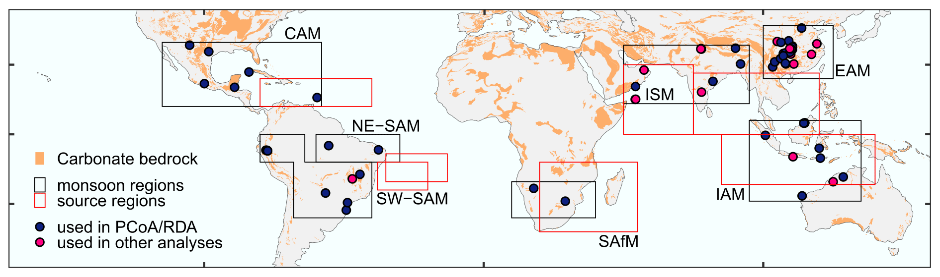
Figure 1 Spatial distribution of speleothem records used is this study. Colours indicate the sites used in principal coordinates analysis (PCoA) and redundancy analysis (RDA) to separate monsoon regions, and sites not used in PCoA and RDA but used in subsequent analyses. The individual regional monsoons are shown by boxes: CAM denotes the Central American monsoon (latitude from 10 to 33^∘, longitude from −115 to −58^∘), SW-SAM denotes the southwestern South American monsoon (latitude from −10 to 0^∘, longitude from −80 to −64^∘; latitude from −30 to −10^∘, longitude −68 to −40^∘), NE-SAM denotes the northeastern South American monsoon (latitude from −10 to 0^∘, longitude: −60 to −30^∘), SAfM denotes the southern African monsoon (latitude from −30 to −17^∘, longitude from 10 to 40^∘), ISM denotes the Indian summer monsoon (latitude from 11 to 32^∘, longitude from 50 to 95^∘), EAM denotes the East Asian monsoon (latitude from 20 to 39^∘, longitude from 100 to 125^∘) and IAM denotes the Indonesian–Australian monsoon (latitude from −24 to 5^∘, longitude from 95 to 135^∘). Source region limits used in the multiple linear regression analysis are also shown. The background carbonate lithology is from the WOrld Karst Aquifer Mapping (WOKAM) project (Goldschneider et al., 2020).

2.2 Climate model simulations

There are relatively few palaeoclimate simulations made with models that incorporate oxygen isotope tracers, and the available simulations do not necessarily focus on the same periods or use the same modelling protocols. Here, we use simulations of opportunity from two isotope-enabled climate models: ECHAM5 (version 5 of the European Centre for medium-range weather forecasting model in HAMburg) and GISS ModelE-R (Goddard Institute for Space Studies Model version E-R). The ECHAM5 simulations provide an opportunity to examine large-scale changes between glacial and interglacial states, using simulations of the MH, LGM and LIG. The GISS ModelE-R ocean–atmosphere coupled general circulation model was used to investigate the evolution of δ¹⁸O evolution during the Holocene, using eight time slice (9, 6, 5, 4, 3, 2, 1 and 0 ka) experiments. Although simulations of the MH 6 ka time slice are available with both models, there are differences in the protocol used for the two experiments which preclude direct comparison of the simulations.

The ECHAM5-wiso MH experiment (Wackerbarth et al., 2012; Werner, 2019) was forced by orbital parameters (based on Berger and Loutre, 1991) and greenhouse gas (GHG) concentrations (CO₂=280 ppm, CH₄=650 ppb, N₂O=270 ppb) appropriate to 6 ka. Changes in sea surface temperature (SST) and sea ice were derived from a transient Holocene simulation (Varma et al., 2012). The control simulation for the MH experiment was an ECHAM-wiso simulation of the period from 1956 to 1999 (Langebroek et al., 2011), using observed SSTs and sea ice cover. This control experiment was forced by SSTs and sea ice only, with atmospheric circulation free to evolve. The ECHAM5-wiso LGM experiment (Werner, 2019; Werner et al., 2018) was forced by orbital parameters (Berger and Loutre, 1991), GHG concentrations (CO₂=185 ppm, CH₄=350 ppb, N₂O=200 ppb), land–sea distribution and ice sheet height and extent appropriate to 21 ka; SST and sea ice cover were prescribed from the GLAMAP dataset (Schäfer-Neth and Paul, 2003). Sea surface water and sea ice δ¹⁸O were uniformly enriched by 1 ‰ at the start of the experiment. The control simulation for the LGM experiment used present-day conditions, including orbital parameters and GHG concentrations set to modern values, and SSTs and sea ice cover from the last 20 years (1979–1999). Both the MH and LGM simulations were run at T106 horizontal grid resolution, approximately $\mathrm{1.1}{}^{\circ }\times \mathrm{1.1}{}^{\circ }$ at the Equator. Comparison of the MH and LGM simulations with speleothem data globally (Figs. S1 and S2 in the Supplement; Comas-Bru et al., 2019) show that the ECHAM model reproduces the broadscale spatial gradients and the sign of isotopic changes at the majority of cave sites (MH: 72 %; LGM: 76 %). However, the changes compared with present are generally more muted in the simulations than shown by the speleothem records.

The LIG experiment (Gierz et al., 2017b, a) was run using the ECHAM5/MPI-OM Earth system model, with stable water isotope diagnostics included in the ECHAM5 atmosphere model (Werner et al., 2011), the dynamic vegetation model JSBACH (Haese et al., 2012) and the MPI-OM ocean–sea-ice module (Xu et al., 2012). This simulation was run at a T31L19 horizontal grid resolution, approximately $\mathrm{3.75}{}^{\circ }\times \mathrm{3.75}{}^{\circ }$. The LIG simulation was forced by orbital parameters derived from Berger and Loutre (1991) and GHG concentrations (CO₂=276 ppm, CH₄=640 ppb, N₂O=263 ppb) appropriate to 125 ka, but it was assumed that the ice sheet configuration and land–sea geography remain unchanged from modern; therefore no change was made to the isotopic composition of sea water. The LIG simulation is compared to a pre-industrial (PI) control with appropriate insolation, GHG and ice sheet forcing for 1850 CE. The sign of simulated isotopic changes in the LIG is in good agreement with ice core records from Antarctica and Greenland and speleothem records from Europe, the Middle East and China (Gierz et al., 2017b), although, as with the MH and LGM, the observed changes tend to be larger than the simulated changes (Fig. S3).

There are GISS ModelE-R (LeGrande and Schmidt, 2009) simulations for eight time slices during the Holocene (9, 6, 5, 4, 3, 2, 1 and 0 ka). The 0 ka experiment is considered as the pre-industrial control (ca. 1880 CE). Orbital parameters were based on Berger and Loutre (1991), and GHG concentrations were adjusted based on ice core reconstructions (Brook et al., 2000; Indermühle et al., 1999; Sowers, 2003) for each time slice. A remnant Laurentide ice sheet was included in the 9 ka simulation, following Licciardi et al. (1998), and the corresponding adjustment was made to mean ocean salinity and ocean water δ¹⁸O to account for this (Carlson et al., 2008). The ice sheet in all the other experiments was specified to be the same as modern; therefore, no adjustment was necessary. The simulations were run using the M20 version of GISS ModelE-R, which has a horizontal resolution of $\mathrm{4}{}^{\circ }\times \mathrm{5}{}^{\circ }$. Each experiment was run for 500 years, and we use the last 100 simulated years for the analyses. Comparison of the simulated trends in δ¹⁸O show good agreement with Greenland ice core records, marine records from the tropical Pacific and Chinese speleothem records (LeGrande and Schmidt, 2009). However, as is the case with the ECHAM simulations, the model tends to produce changes that are less extreme than those shown by the observations (Figs. S4, S5, S6).

2.3 Principal coordinate analysis and redundancy analysis

We used PCoA to identify regionally coherent patterns in the speleothem δ¹⁸O records for the Holocene. PCoA is a multivariate ordination technique that uses a distance matrix to represent inter-object (dis)similarity in reduced space (Gower, 1966; Legendre and Legendre, 1998). Speleothem records from individual sites are often discontinuous; missing data are problematic for many ordination techniques. PCoA is more robust to missing data than other methods (Kärkkäinen and Saarela, 2015; Rohlf, 1972). We used a correlation matrix of speleothem records as the (dis)similarity measure. The temporal resolution of speleothem records was first standardised by calculating a running average mean with non-overlapping 500-year windows. This procedure produces a single composite record when there are several records for a given site. PCoA results were displayed as a biplot, where sites ordinated close to one another (i.e. with similar PCoA scores) show similar Holocene trends, and sites ordinated far apart have dissimilar trends. We used the “broken stick” model (Bennett, 1996) to identify which PCoA axes were significant. We used redundancy analysis (RDA: Legendre and Legendre, 1998; Rao, 1964) with latitude and longitude as predictor variables to identify if PCoA (dis)similarities were related to geographical location, and principal components analysis (PCA) to identify the main patterns of variation. As these explanatory variables are not dimensionally homogeneous, they were centred on their means and standardised to allow direct comparison of the gradients. PCoA and RDA analyses were carried out using the “vegan” package in R (Oksanen et al., 2019).

2.4 Glacial–interglacial changes in δ¹⁸O

We examined shifts in δ¹⁸O_spel observations and in annual precipitation-weighted mean δ¹⁸O_precip from ECHAM-wiso in regions influenced by the monsoon, between the MH, LGM and LIG. Values are given as anomalies with respect to the present day for speleothems or the control simulation experiment for model outputs. Comas-Bru et al. (2019) have shown that differences in speleothem δ¹⁸O data between the 20th century and the pre-industrial period (i.e. 1850±15 CE) are within the temporal and measurement uncertainties of the data; thus, the use of different reference periods (i.e. PI for the ECHAM LIG experiment, 20th century for ECHAM MH, LGM experiments) should have little effect on our analyses. We used mean site δ¹⁸O_spel values for each period for the regions identified in the PCoA analysis. Where there are multiple speleothem δ¹⁸O records for a site in a time period, they were averaged to calculate mean δ¹⁸O_spel. Three sites above 3500 m were excluded from the calculation of the means because high-elevation sites have more negative δ¹⁸O values than their low-elevation counterparts, and their inclusion would distort the regional estimates.

There are relatively few speleothems covering both the present day and the period of interest (i.e. MH, LGM or LIG), precluding the calculation of δ¹⁸O_spel anomalies from the speleothem data. Therefore, we calculated anomalies with respect to the modern period (1960–2017 CE) using the Online Isotopes in Precipitation Calculator (OIPC: Bowen, 2018; Bowen and Revenaugh, 2003), a global gridded dataset of interpolated mean annual precipitation-weighted δ¹⁸O_precip data, as reference. This dataset combines data from 348 stations from the Global Network of Isotopes in Precipitation (IAEA/WMO, 2018), covering part or all of the 1960–2014 period, and other records available at the Waterisotopes Database (Waterisotopes Database, 2017).

OIPC δ¹⁸O_precip was converted to its speleothem equivalent assuming that (i) precipitation-weighted mean annual δ¹⁸O_precip is equivalent to mean annual drip-water δ¹⁸O (Yonge et al., 1985) and that (ii) precipitation of calcite is consistent with the empirical speleothem-based kinetic fractionation factor of Tremaine et al. (2011) and precipitation of aragonite follows the fractionation factor from Grossman and Ku (1986), as formulated by Lachniet (2015):

$$\begin{array}{}\text{(1)}& \begin{array}{rl}& {\mathit{\delta }}^{\mathrm{18}}{\mathrm{O}}_{\mathrm{calcite}\mathrm{\_}\mathrm{SMOW}}=w{\mathit{\delta }}^{\mathrm{18}}{\mathrm{O}}_{\mathrm{precip}\mathrm{\_}\mathrm{SMOW}}\\ & +\left(\left({\displaystyle \frac{\mathrm{16.1}\cdot \mathrm{1000}}{T}}\right)-\mathrm{24.6}\right)\left(T\text{in}\mathrm{K}\right),\end{array}\end{array}$$

$$\begin{array}{}\text{(2)}& \begin{array}{rl}& {\mathit{\delta }}^{\mathrm{18}}{\mathrm{O}}_{\mathrm{aragonite}\mathrm{\_}\mathrm{SMOW}}=w{\mathit{\delta }}^{\mathrm{18}}{\mathrm{O}}_{\mathrm{precip}\mathrm{\_}\mathrm{SMOW}}\\ & +\left(\left({\displaystyle \frac{\mathrm{18.34}\cdot \mathrm{1000}}{T}}\right)-\mathrm{31.954}\right)\left(T\text{in}\mathrm{K}\right),\end{array}\end{array}$$

where δ¹⁸O_{calcite_SMOW} and δ¹⁸O_{aragonite_SMOW} are the respective speleothem isotopic composition for calcite and aragonite speleothems with reference to the VSMOW (Vienna Standard Mean Ocean Water) standard (in per mille), wδ¹⁸O_precip is the OIPC precipitation-weighted annual mean isotopic composition of precipitation with respect to the VSMOW standard and T is the mean annual cave temperature (in kelvin). We used the long-term (1960–2016) mean annual surface air temperature from the CRU-TS4.01 database (Harris and Jones, 2017; Harris et al., 2020) at each site as a surrogate for mean annual cave air temperature. The resolution of the gridded data means that wδ¹⁸O_{precip_SMOW} and T may be the same for nearby sites.

We use the VSMOW to VPDB (Vienna Pee Dee Belemnite) conversion from Coplen et al. (1983), which is independent of speleothem mineralogy:

$$\begin{array}{}\text{(3)}& {\mathit{\delta }}^{\mathrm{18}}{\mathrm{O}}_{\mathrm{PDB}}=\mathrm{0.97001}\cdot {\mathit{\delta }}^{\mathrm{18}}{\mathrm{O}}_{\mathrm{SMOW}}-\mathrm{29.29},\end{array}$$

where δ¹⁸O_PDB is relative to the VPDB standard, and δ¹⁸O_SMOW is relative to VSMOW standard.

Average uncertainties in the speleothem age–depth models are ∼50 years during the Holocene. This interval is smaller than the time windows used in this analysis; therefore, the age uncertainty is expected to have a negligible impact on the results. We investigated the influence of age uncertainties on the LGM and LIG δ¹⁸O_spel anomalies by examining the impact of using different window widths (±500, ±700, ±1000, ±2000 years) on the regional mean δ¹⁸O_spel anomalies.

We used anomalies of wδ¹⁸O_precip, mean annual surface air temperature (MAT) and mean annual precipitation (MAP) from the ECHAM5-wiso simulations to investigate the changes in δ¹⁸O_spel between the MH, LGM and LIG as well as their association with changes in climate. Values were calculated from land grid cells (>50 % land) ±3^∘ around each speleothem site. This distance was chosen with reference to the coarsest-resolution simulation (LIG, ca. $\mathrm{3.75}{}^{\circ }\times \mathrm{3.75}{}^{\circ }$). Gridded values of MAT and MAP were weighted by the proportion of each grid cell that lies within ±3^∘ of the site, and linear distance-weighted means were calculated for each site and time slice. We only considered regions with at least one speleothem record for each of the three time periods, although these were not required to be the same sites, and where the observed shifts in δ¹⁸O_spel were in the same direction and of a similar magnitude to the simulated wδ¹⁸O_precip.

2.5 Holocene and Last Interglacial regional trends

Regional speleothem δ¹⁸O changes through the Holocene were examined by creating composite time series for each region identified in the PCoA analysis with at least four Holocene records (>5000 years long). Regional composites were constructed using a four-step procedure, modified from Marlon et al. (2008):

1. The δ¹⁸O data for individual speleothems were transformed to z scores, so all records have a standardised mean and variance:

   $$\begin{array}{}\text{(4)}& z{\text{score}}_i=\left({{\mathit{\delta }}^{\mathrm{18}}\mathrm{O}}_i-\stackrel{\mathrm{‾}}{{\mathit{\delta }}^{\mathrm{18}}{\mathrm{O}}_{\left(\mathrm{base}\mathrm{period}\right)}}\right)/s{\mathit{\delta }}^{\mathrm{18}}{\mathrm{O}}_{\left(\mathrm{base}\mathrm{period}\right)},\end{array}$$

   where $\stackrel{\mathrm{‾}}{{\mathit{\delta }}^{\mathrm{18}}\mathrm{O}}$ is the mean, and sδ¹⁸O is the standard deviation of δ¹⁸O for a common base period. A base period of 7000 to 3000 years BP was chosen to maximise the number of records included in each composite.

2. The standardised data for a site were resampled by applying a 100-year non-overlapping running mean with the first bin centred at 50 years BP, in order to create a single site time series while ensuring that highly resolved records do not dominate the regional composite.

3. Each regional composite was constructed using locally weighted regression (Cleveland and Devlin, 1988) with a window width of 3000 years and fixed target points in time.

4. Confidence intervals (5th and 95th percentiles) for each composite were generated by bootstrap resampling by site over 1000 iterations.

There are too few sites to construct regional composites for the peak of the LIG (Marine Isotope Stage 5e); thus, the trends in δ¹⁸O_spel were examined using records from individual sites covering the period from 130 to 116 ka BP.

We calculated Holocene regional composites from annual precipitation-weighted mean δ¹⁸O_precip anomalies simulated by the GISS model. Simulated δ¹⁸O_precip trends were calculated using linear distance-weighted mean δ¹⁸O_precip values from land grid cells (>50 % land) within ±4^∘ around each site. This distance was determined by the grid resolution of the model. Regional composites were then produced using bootstrap resampling in the same way as for the speleothem data. The simulated anomalies are relative to the control run rather than the specified base period used for the speleothem-based composites, so absolute values of simulated and observed Holocene trends are expected to differ. Preliminary analyses showed that neither the mean values nor trends in δ¹⁸O_precip were substantially different if the sampled area was reduced to match the sampling used for the ECHAM-based box plot analysis, or was increased to encompass the larger regions shown in Fig. 1 and used in the multiple regression analysis.

2.6 Multiple regression analysis

We investigate the underlying relationships between regional δ¹⁸O_precip (and by extension δ¹⁸O_spel and monsoon climate through the Holocene using multiple linear regression (MLR). We use annual precipitation-weighted mean δ¹⁸O_precip anomalies and climate variables from GISS ModelE-R. Climate variables were chosen to represent the four potential large-scale drivers of regional changes in the speleothem δ¹⁸O records. Specifically, we use changes in mean precipitation and precipitation recycling over the monsoon regions, and changes in mean surface air temperature and surface wind direction over the moisture source regions. Whereas the influence of changes in precipitation, recycling and temperature are relatively direct measures, the change in surface wind direction over the moisture source region is used as an index of potential changes in the moisture source region and transport pathway. The boundaries of each monsoon region (Fig. 1) were defined to include all the speleothem sites used to construct the Holocene δ¹⁸O_spel composites. Moisture source area limits (Fig. 1) were defined based on moisture tracking studies (Bin et al., 2013; Breitenbach et al., 2010; D'Abreton and Tyson, 1996; Drumond et al., 2008, 2010; Durán-Quesada et al., 2010; Kennett et al., 2012; Nivet et al., 2018; Wurtzel et al., 2018) and GISS simulated summer surface winds. All climate variables were extracted for the summer months, defined as May to September (MJJAS) for Northern Hemisphere regions and November to March (NDJFM) for Southern Hemisphere regions (Wang and Ding, 2008) on the basis that these regions are dominated by summer season precipitation (Fig. S7). Only grid cells with >50 % land were used to extract variables over monsoon regions, and only grid cells with <50 % land were used to extract variables over moisture source regions. The inputs to the MLR for each time interval were calculated as anomalies from the control run.

Precipitation recycling was calculated as the ratio of locally sourced precipitation versus total precipitation. Although the GISS ModelE-R mid-Holocene experiment explicitly estimates recycling using vapour source distribution tracers (Lewis et al., 2014), this was not done for all the Holocene time slice simulations. Therefore, we calculate a precipitation recycling index (RI), following Brubaker et al. (1993):

$$\begin{array}{}\text{(5)}& \text{RI}={\displaystyle \frac{P_{\mathrm{R}}}{P}}={\displaystyle \frac{E}{\mathrm{2}{Q}_{\mathrm{H}}+E}},\end{array}$$

where locally sourced (recycled) precipitation (P_R) is estimated using total evaporation over a region (E), and total precipitation (P) is estimated as the sum of total evaporation and net incoming moisture flux integrated across the boundaries of the region (Q_H). Therefore, RI expresses the change in the contribution of local, recycled precipitation independently of any overall change in precipitation amount.

We incorporate mean meteorological variables and δ¹⁸O_precip for all Holocene time slices (1 to 9 ka) and all monsoon regions into the MLR model. Thus, the relationships constrained by the overall (global) MLR model represent the combined response across all monsoon regions. We use the pseudo-R² to determine the goodness of fit for the global MLR model and t values (the regression coefficient divided by its standard error) to determine the strength of each relationship. Partial residual plots were used to show the relationship between each predictor variable and δ¹⁸O_precip when the effects of the other variables are held constant.

All statistical analyses were performed in R (R Core Team, 2019), and plots were generated using ggplot (Wickham, 2016).

3 Results

3.1 Principal coordinate analysis and redundancy analysis

PCoA shows the (dis)similarity of Holocene δ¹⁸O_spel evolution across individual records and, thus, allows an objective regionalisation of these records. The first two PCoA axes are significant, according to the broken stick test, and account for 65 % and 20 % of δ¹⁸O_spel variability respectively (Table 1). The PCoA scores differentiate records geographically (Fig. 2a): Southern Hemisphere monsoon regions such as the southwestern South American monsoon (SW-SAM) and South African monsoon (SAfM) are characterised by low PCoA1 scores, whereas Northern Hemisphere monsoons such as the Indian summer monsoon (ISM) and the East Asian monsoon (EAM) are characterised by higher PCoA1 scores. This indicates that regions can be differentiated based on their temporal evolution as captured by the first PCoA axis. Most Southern Hemisphere regions also have lower PCoA2 scores, although this is not consistent over time. Speleothem records from the Central American monsoon (CAM) and the Indonesian–Australian monsoon (IAM) have PCoA scores that are an intermediate between the Northern Hemisphere and Southern Hemisphere regions. PCoA clearly separates the South American records into a northeastern region (NE-SAM), with scores similar to other Northern Hemisphere monsoon regions, and a southwestern region (SW-SAM), with scores similar to other Southern Hemisphere regions. The RDA supports a geographical control on the (dis)similarity of speleothem δ¹⁸O records over the Holocene (Fig. 2b). RDA1 explains 37 % of the variability and is significantly correlated with both latitude and longitude (Table 2).

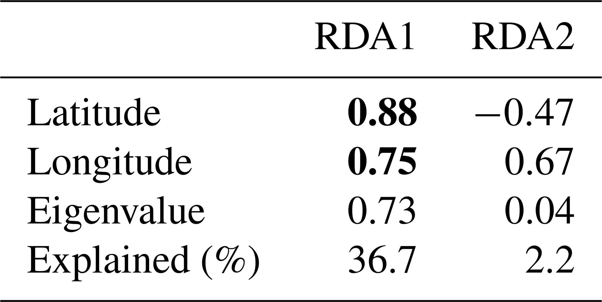
Table 1 Results of the principal coordinates analysis (PCoA). Significant axes, as determined by the broken stick method (Bennett, 1996), are shown in bold.

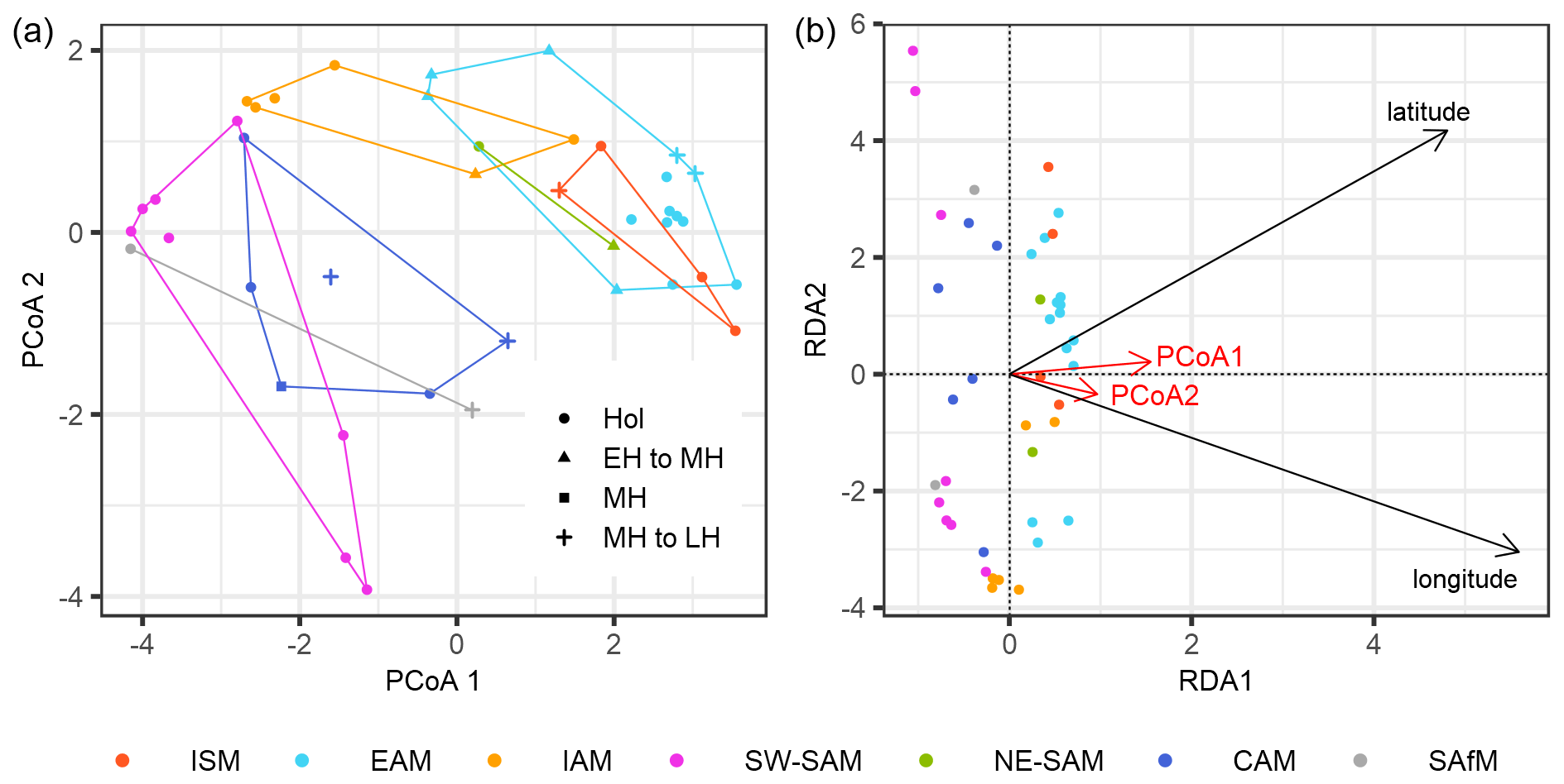
Figure 2 Results of the principal coordinate analysis (PCoA) and redundancy analysis (RDA). (a) PCoA biplot showing the loadings of each site on the first two axes, which represent 85 % of the total variance. Shapes indicate the Holocene coverage of each site, where sites with a coverage ≥8000 years represent most or all of the Holocene (Hol). Sites with a temporal coverage of <8000 years are coded to show whether they represent the early Holocene to mid-Holocene (EH to MH; record midpoint >8000 years BP), the mid-Holocene (MH; record midpoint between 8000 and 5000 years BP) or the mid-Holocene to late Holocene (LH to MH; midpoint <5000 years BP). (b) RDA triplot, where the response variables are the PCoa1 and PCoA2 axes explained by latitude and longitude. The direction of the PCoA axes have been fixed so that they align with the explanatory variables.

Table 2 Results of the redundancy analysis (RDA). Variables that are significantly correlated (P <0.01) with the RDA axes are shown in bold.

3.2 Regional interglacial–glacial differences

To investigate the causes of shifts in δ¹⁸O between the MH, LGM and LIG, we compare simulated and observed regional δ¹⁸O signals during these periods with shifts in climate variables (precipitation and temperature). Only the ISM, EAM and IAM regions have sufficient speleothem data (i.e. at least one record from every time period) to allow comparisons across the MH, LGM and LIG (Fig. 3) and have similar shifts in observed δ¹⁸O_spel and simulated δ¹⁸O_precip. The regional mean δ¹⁸O_spel anomalies calculated for different time windows (±500, ±700, ±1000, ±2000 years) vary by less than 0.35 ‰ for the LGM (ISM: <0.16 ‰; EAM: <0.35 ‰; IAM: <0.22 ‰) and 0.48 ‰ for the LIG (ISM: <0.16 ‰; EAM: <0.48 ‰; IAM: <0.11 ‰), indicating that age uncertainties have a minimal impact on these mean values. The most positive δ¹⁸O_spel anomalies in all three regions occur at the LGM, with more negative anomalies for the MH and LIG. The simulated δ¹⁸O_precip anomalies show a similar pattern, with more positive anomalies during the LGM than during the MH or the LIG. The amplitude of this pattern is also similar between δ¹⁸O_precip and δ¹⁸O_spel, when the observations are converted to their drip water equivalent (Fig. S8). The differences in regional δ¹⁸O_spel anomalies between MH and LIG differ across the three regions. In both the ISM and the EAM, differences in δ¹⁸O_spel values between the MH and LIG are small (Fig. 3a, b), although ISM LIG δ¹⁸O_spel values are slightly more negative than MH values. In the IAM, MH values are less negative than the LIG (Fig. 3c). However, there are only a limited number of speleothem records from the ISM and IAM during the LIG, so the apparent differences between the two intervals in these regions may not be meaningful. Glacial–interglacial shifts are also seen in simulated temperature and precipitation, with warmer and wetter conditions during interglacials and cooler and drier conditions during the LGM in all three regions. Differences in simulated precipitation between the MH and the LIG could help explain the differences between δ¹⁸O_spel in the ISM and IAM, as the LIG is wetter than the MH in the ISM and drier than the MH in the IAM. However, the LIG is also drier than the MH in the EAM, a feature that appears inconsistent with the lack of differentiation between the δ¹⁸O signals in this region.

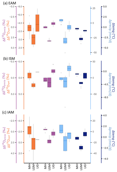
Figure 3 Speleothem δ¹⁸O anomalies compared to anomalies of δ¹⁸O_precip, precipitation and temperature from the ECHAM simulations for the (a) East Asian (EAM), (b) Indian (ISM) and (c) Indonesian–Australian (IAM) monsoons. The boxes show the median value (line) and the interquartile range, and the whiskers show the minimum and maximum values, with outliers represented by grey dots. Note that the isotope axes are reversed, so that the most negative anomalies are at the top of the plot, to be consistent with the assumed relationship with the direction of change in precipitation and temperature.

3.3 Regional-scale interglacial δ¹⁸O evolution

There are four monsoon regions with sufficient data to examine regional Holocene δ¹⁸O trends: EAM, ISM, SW-SAM and IAM (Fig. 4). The IAM region has the fewest records (n=7), whereas the EAM has the largest number of records (n=14). The regional composites are expressed as z scores, i.e. changes with respect to the mean and variance of δ¹⁸O for the base period (3000–7000 years BP). The confidence intervals on the regional composites are small for all regions, except SW-SAM in the early Holocene. The EAM and ISM regions (Fig. 4a–e) show the most positive δ¹⁸O_spel z scores around 12 ka followed by a rapid decrease towards their most negative values at ∼9.5 and ∼9 ka respectively. The δ¹⁸O_spel z scores in the EAM are relatively constant from 9.5 to ∼7 ka, whereas this plateau is present but less marked in the ISM. There is a gradual trend towards more positive δ¹⁸O_spel z scores towards the present in both regions thereafter. The SW-SAM records (Fig. 4i) have their most positive δ¹⁸O_spel z scores in the early Holocene with a gradual trend to more negative scores towards the present. By contrast, the IAM z scores (Fig. 4g) are most positive at 12 ka, gradually decrease until ca. 5 ka and are relatively flat thereafter.

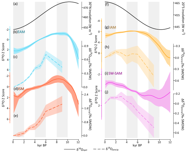
Figure 4 Evolution of regional speleothem δ¹⁸O signals through the Holocene compared to δ¹⁸O_precip simulated by the GISS model. Panels (a–e) show Northern Hemisphere monsoons (EAM denotes the East Asian monsoon; ISM denotes the Indian summer monsoon) and summer (May through September) insolation at 30^∘ N (Berger, 1978). Panels (f–j) show Southern Hemisphere monsoons (SW-SAM denotes the southwestern South American monsoon; IAM denotes the Indonesian–Australian monsoon) and summer (November through March) insolation for 20^∘ S (Berger, 1978). The speleothem δ¹⁸O changes are expressed as z scores, with a smoothed loess fit (3000-year window), and confidence intervals obtained by bootstrapping by site. δ¹⁸O_precip values are expressed as anomalies from the pre-industrial control simulation. Note that the isotope axes are reversed, so that the most negative anomalies are at the top of the plot, to be consistent with the assumed relationship with the changes in insolation.

There are insufficient data to create composite curves for the LIG, but individual records from the four regions (Fig. 5) show similar features to the Holocene trends. Records from the ISM and EAM (Fig. 5 left), for example, are characterised by an initial sharp decrease in δ¹⁸O_spel values of about 4 ‰ between 130 and 129 ka, and most of the records (Dykoski et al., 2005; Kathayat et al., 2016; Wang et al., 2008) then show little variability for several thousand years. Despite the fact that the Tianmen record (Cai et al., 2010, 2012) shows considerable variability between 123 and 127 ka, there is nevertheless a similar plateau in the average observed value before the rapid change to less negative values after 127 ka. Similar to the Holocene, the SW-SAM record (Cheng et al., 2013) shows increasingly negative δ¹⁸O_spel values through the LIG. The trend shown for Whiterock Cave (Carolin et al., 2016) also displays similar features to the IAM Holocene composite, with a gradual trend towards more negative values initially and a relatively complacent curve towards the end of the interglacial (Fig. 5 right).

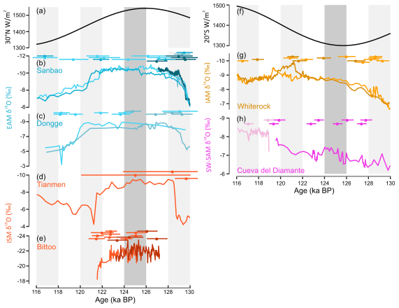
Figure 5 Comparison of changes in summer insolation and δ¹⁸O_spel through the peak of the Last Interglacial (Marine Isotope Stage 5e) from the (b, c) East Asian monsoon (EAM), (d, e) Indian summer monsoon (ISM), (g) southwestern South American monsoon (SW-SAM) and (h) Indonesian–Australian monsoon (IAM) regions. The U–Th dates and uncertainties are shown for each record. The summer insolation curves (Berger, 1978) are for May through September at 30^∘ N in the Northern Hemisphere (a) and for November through March for 20^∘ S in the Southern Hemisphere (f). Note that the isotope axes are reversed, so that the most negative anomalies are at the top of the plot, to be consistent with the assumed relationship with the changes in insolation. The LIG (Marine Isotope Stage 5e) time slice used in the analysis in Sect. 2.4 is shown by the dark-grey bar.

3.4 Multiple regression analysis of Holocene δ¹⁸O_precip

The MLR analyses of simulated δ¹⁸O_precip trends identify the impact of an individual climate variable on δ¹⁸O_precip in the absence of changes in other variables. The global MLR model includes the Holocene (1–9 ka) δ¹⁸O_precip trends combined across all monsoon regions (CAM, ISM, EAM, SW-SAM, NE-SAM, SAfM, IAM). This global monsoon MLR model has a pseudo-R² of 0.80 and shows statistically significant relationships between the anomalies in δ¹⁸O_precip and anomalies in regional precipitation, temperature and surface wind direction (Table 3). The partial residual plots (Fig. 6) show there is a strong negative relationship with regional precipitation (t value of −8.75) and a strong positive relationship (t value of 8.03) with surface wind direction over the moisture source region, an index of changes in either source area or moisture pathway. This indicates that increases in regional precipitation alone will lead to a decrease in δ¹⁸O, whereas changes in source area and/or moisture pathway, in the absence of changes in other variables, will lead to a significant change in δ¹⁸O. The relationship with temperature over the moisture source region is weaker, but positive (t value of 2.05), i.e. an increase in temperature over the moisture source region will lead to an increase in δ¹⁸O if there are no changes in other climate variables. Precipitation recycling is not significant in this global analysis. The exact choice of source region has a negligible impact on the model – for example, expanding the ISM source region to include the Bay of Bengal does not change the outcome of this analysis (Fig. S9, Table S1).

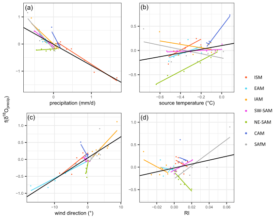
Figure 6 Partial residual plots from the multiple linear regression analysis, showing the relationship between anomalies in simulated δ¹⁸O_precip and the four predictor variables, after considering the fitted partial effects of all the other predictors. The simulated δ¹⁸O_precip values are anomalies relative to the pre-industrial control simulation and are annual values weighted by precipitation amount. The predictor variables are precipitation in the delineated monsoon region (mm d⁻¹), temperature in the source region (^∘C), surface wind direction over the source region (^∘) as an index of potential changes in source region and the ratio of precipitation recycling to total precipitation over the monsoon region (RI, unitless). The predictor variables are summer mean values, representing the summer monsoon, where summer is defined as May to September for the Northern Hemisphere monsoons and November to March for the Southern Hemisphere monsoons.

Table 3 Results of the multiple linear regression analysis. Significant relationships (P <0.01) are shown in bold.

There are too few data points to make regressions for individual monsoon regions, but the distribution of data points for each region in the partial residual plots (Fig. 6) is indicative of the degree of conformity to the global MLR model (representing the combined response across all monsoon regions). Data points from the ISM, SW-SAM, IAM and SAfM are well aligned with the overall relationship with regional precipitation (Fig. 6a), indicating that precipitation is an important control on changes in δ¹⁸O_precip in these regions. The NE-SAM, EAM and CAM values deviate somewhat from the overall relationship and, although there are relatively few points, this suggests that changes in precipitation are a less important influence on δ¹⁸O_precip changes in these regions. The impact of temperature changes (Fig. 6b) in the ISM, EAM and SW-SAM is broadly consistent with the overall relationship. The slope of the relationship with temperature is negative for the IAM and NE-SAM, and as this is physically implausible, it suggests that some factor not currently included in the MLR is influencing these records. However, the inconsistencies between the regional signals helps to explain why the global relationship between anomalies in temperature and δ¹⁸O_precip is weak (Fig. 6b) and probably reflects the fact that tropical temperature changes during the Holocene are small. Data points from the EAM, ISM and IAM are well aligned with the overall relationship between changes in δ¹⁸O_precip and changes in wind direction (Fig. 6c), indicating that changes in source area or moisture pathway are an important control on changes in δ¹⁸O_precip in these regions. However, values for CAM, SW-SAM, NE-SAM and SAfM deviate strongly from the overall relationship. Recycling does not appear to be an important contributor to changes in δ¹⁸O_precip except in SW-SAM and SAfM (Fig. 6d).

4 Discussion

We have shown that it is possible to derive an objective regionalisation of speleothem records based on the PCoA of the oxygen-isotope trends through the Holocene (Fig. 2). This approach separates out regions with a distinctive Northern Hemisphere signal (e.g. ISM, EAM, NE-SAM) from regions with a distinctive Southern Hemisphere signal (e.g. SW-SAM, SAfM), reflecting the fact that the evolution of regional monsoons in each hemisphere follows, to some extent, insolation forcing. It also identifies regions that have an intermediate pattern (e.g. IAM). The robustness of the regionalisation is borne out by the fact that Holocene composite trends from each region have tight confidence intervals (Fig. 4), showing that the signals of individual records across a region show broad similarities. The monsoon regions identified by PCoA are consistent with previous studies (Wang et al., 2014). The tracking of Northern Hemisphere insolation is a recognised feature of monsoon systems in India and China (see reviews by Kaushal et al., 2018; Zhang et al., 2019). The separation of speleothem records from NE-SAM from those in SW-SAM is consistent with the precipitation dipole that exists between northeastern Brazil (Nordeste) and the continental interior (Berbery and Barros, 2002; Boers et al., 2014). The anti-phasing of speleothem records from the two regions during the Holocene has been recognised in previous studies (Cruz et al., 2009; Deininger et al., 2019). The intermediate nature of the records from the maritime continent is consistent with the fact that the Indonesian–Australian (IAM) summer monsoon is influenced by cross-equatorial air flow and, hence, can be influenced by Northern Hemisphere conditions (Trenberth et al., 2000). Palaeoenvironmental records from this region show mixed signals for the Holocene: some have been interpreted as showing enhanced (Beaufort et al., 2010; Mohtadi et al., 2011; Quigley et al., 2010; Wyrwoll and Miller, 2001) and others reduced precipitation (Kuhnt et al., 2015; Steinke et al., 2014) during the early and mid-Holocene. Modelling studies have shown that this region is highly sensitive to SST changes in the Indian Ocean and South China Sea, which in turn reflect changes in the Northern Hemisphere winter monsoons. Although most climate models produce a reduction in precipitation across the IAM during the mid-Holocene in response to orbital forcing, this is less than might be expected in the absence of ocean feedbacks associated with changes in the Indian Ocean (Zhao and Harrison, 2012).

The separation of northern and southern monsoon regions is consistent with the idea that changes in monsoon rainfall are primarily driven by changes in insolation (Ding and Chan, 2005; Kutzbach et al., 2008). Indeed, regional δ¹⁸O_spel composites from the EAM, ISM and SW-SAM show a clear relationship with the long-term trends in local summer insolation (Fig. 4). Similar patterns are seen in individual speleothem records from each region confirming that the composite trends are representative. However, the composite trends are not an exact mirror of the insolation signal over the Holocene. For example, the ISM and EAM composites show a more rapid rise during the early Holocene than implied by the insolation forcing. The maximum wet phase in these two regions lasts for ca. 3000 years, again contrasting with the gradual decline in insolation forcing after its peak at ca. 11 ka. Both the rapid increase and the persistence of wet conditions for several thousand years is also observed in other palaeohydrological records across southern and central China, including pollen (Zhao et al., 2009; Li et al., 2018) and peat records (Hong et al., 2003; Zhou et al., 2004). These features are also characteristic of lake records from India (Misra et al., 2019). The lagged response to increasing insolation is thought to be due to the presence of Northern Hemisphere ice sheets in the early Holocene (Zhang et al., 2018). The persistence of wetter conditions through the early and mid-Holocene is thought to reflect the importance of land surface and ocean feedbacks in sustaining regional monsoons (Dallmeyer et al., 2010; Kutzbach et al., 1996; Marzin and Braconnot, 2009; Rachmayani et al., 2015; Zhao and Harrison, 2012). The evolution of regional monsoons during the LIG shows patterns similar to those observed during the Holocene, including the lagged response to insolation and the persistence of wet conditions after peak insolation. This is again consistent with the idea that internal feedbacks play a role in modulating the monsoon response to insolation forcing. We have also shown that there is little difference in the isotopic values between the MH and the LIG in the ISM and EAM regions, which is also observed in individual speleothem records (Kathayat et al., 2016; Wang et al., 2008). The LIG (125 ka) period was characterised by higher summer insolation, higher CO₂ concentrations (Otto-Bliesner et al., 2017) and lower ice volumes (Dutton and Lambeck, 2012) than the MH, suggesting that the LIG ISM and EAM monsoons should be stronger than the MH monsoons. The lack of a clear differentiation in the isotope signals between the LIG and MH suggests that other factors play a role in modulating the monsoon response to these forcings and may reflect the importance of global constraints on the externally forced expansion of the tropical circulation (Biasutti et al., 2018).

Global relationships between δ¹⁸O_precip and climate variables (precipitation amount, temperature and surface wind direction; Fig. 6) are consistent with existing studies: a strong relationship with precipitation and a weaker temperature effect have been widely observed at tropical and subtropical latitudes in modern observations (Dansgaard, 1964; Rozanski et al., 1993). The significant global relationship between δ¹⁸O_precip and surface winds supports the idea that changes in moisture source and pathway are also important for explaining δ¹⁸O variability over the Holocene. The multiple regression analysis also provides insights into the relative importance of different influences at a regional scale. In the ISM, the results support existing speleothem studies which suggest that changes in precipitation amount (Cai et al., 2015; Fleitmann et al., 2004) and to a lesser extent moisture pathway (Breitenbach et al., 2010) drive δ¹⁸O_spel variability. The δ¹⁸O variability in the IAM region through the Holocene also appears to be strongly driven by changes in precipitation and moisture pathway, consistent with the interpretation of Wurtzel et al. (2018). Changes in regional precipitation (where the cave sites are located) do not seem to explain the observed changes in δ¹⁸O_spel in the EAM during the Holocene, where Holocene δ¹⁸O_precip evolution is largely driven by changes in atmospheric circulation (indexed by changes in surface winds). This is consistent with existing studies that emphasise changes in moisture source and/or pathway rather than local precipitation changes (Maher, 2016; Maher and Thompson, 2012; Tan, 2014; Yang et al., 2014). Speleothem δ¹⁸O records in the SW-SAM clearly reflect regional-scale changes in precipitation, consistent with interpretations of individual records (Cruz et al., 2009; Kanner et al., 2013). However, this is a region where changes in precipitation recycling also appear to be important. Based on regional water budget estimates, recycling presently contributes ca. 25 %–35 % of the precipitation over the Amazon (Brubaker et al., 1993; Eltahir and Bras, 1994); these figures increase up to ca. 40 %–60 % based on moisture tagging studies (Risi et al., 2013; Yoshimura et al., 2004).

The LGM is characterised by lower Northern Hemisphere summer insolation, globally cooler temperatures, expanded global ice volumes and lower GHG concentrations than either the MH or the LIG. The MH and LIG (Marine Isotope Stage 5e) periods represent peaks in the present and last interglacial periods, whereas the LGM represents maximum ice extent during the Last Glacial Period. Hence, comparison of these time periods provides a snapshot view of glacial–interglacial variability. The δ¹⁸O_spel anomalies are more positive during the LGM than during the MH or LIG, suggesting drier conditions in the ISM, EAM and IAM, supported by simulated changes in δ¹⁸O_precip and precipitation (Fig. 3). Cooler SSTs of approximately 2 ^∘C (relative to the MH and LIG) in the ISM and EAM and of approximately 3 ^∘C in IAM source areas, along with a ca. 5 % decrease in relative humidity (Yue et al., 2011), would result in a water vapour δ¹⁸O signal at the source that is ca. 1 ‰ more depleted than seawater. This depletion results from the temperature dependence of equilibrium fractionation during evaporation and kinetic isotope effects related to humidity (Clark and Fritz, 1997). This fractionation counteracts any impact from enriched seawater δ¹⁸O values during the LGM (ca. +1 ‰ relative to the MH or LIG; Waelbroeck et al., 2002). Cooler air temperatures will also result in a depletion of δ¹⁸O_spel during the LGM of ca. 0.4 ‰ and 0.6 ‰ for the ISM/EAM and IAM respectively, as a result of water–calcite (or water–aragonite) fractionation (Grossman and Ku, 1986; Tremaine et al., 2011). This has the effect of slightly reducing the regional LGM δ¹⁸O_spel signals, although the change is small and within the uncertainty of the regional signals. Enriched δ¹⁸O_precip and δ¹⁸O_spel values during the LGM must therefore be caused by a significant decrease in atmospheric moisture and precipitation that resulted from the cooler conditions.

We have used version 2 of the SISAL database (Atsawawaranunt et al., 2018; Comas-Bru et al., 2020a) in our analyses. Despite the fact that SISALv2 includes more than 70 % of known speleothem isotope records, there are still too few records from some regions (e.g. Africa, the Caribbean) to make meaningful analyses. The records for older time periods are also sparse. For example, there are only 14 records from monsoon regions covering the LIG in SISALv2. Nevertheless, our analyses show that there are robust and explicable patterns for most monsoon regions during the Holocene and sufficient records to make meaningful analyses of the LGM and LIG. Whilst there is a need for the generation of new speleothem records from key regions such as northern Africa, further expansion of the SISAL database will certainly provide additional opportunities to analyse the evolution of the monsoons through time.

The impact of age uncertainties, included in SISALv2, are not taken into account in our analyses. Age uncertainties during the Holocene are smaller than the interval used for binning records and the width of the time windows used and, thus, should not have a significant effect on our conclusions. The mean age uncertainty at the LGM and LIG is ca. 430 and 1140 years respectively. However, varying the window length for the selection of LGM and LIG samples from ±500 to ±2000 years, thereby encompassing this uncertainty, has a negligible effect (<0.5 ‰) on the average δ¹⁸O values. Thus, the interglacial–glacial contrast in regional δ¹⁸O_spel is also robust to age uncertainties.

Isotope-enabled climate models are used in this study to explore observed regional-scale trends in δ¹⁸O_spel. There is a limited number of isotope-enabled models, and there are no simulations of the same time period using the same experimental protocol. Although there are simulations of the MH from both ECHAM5-wiso and GISS, for example, these models have different grid resolutions and used different boundary conditions. This could help to explain why the two models yield different estimates of the change in regional δ¹⁸O_precip (of 0.5 ‰) at the MH. However, both models show trends in δ¹⁸O_precip that reproduce the observed changes in regional δ¹⁸O_spel (Figs. 3, 4), and this provides a basis for using these models to explore the causes of these trends on different timescales. The failure to reproduce the LGM δ¹⁸O_spel signal in SW-SAM in the ECHAM5-wiso model, which precluded a consideration of interglacial–glacial shifts in this region, is a common feature of other isotope-enabled simulations (Caley et al., 2014; Risi et al., 2010). Identifying the underlying relationships between δ¹⁸O_precip and monsoon climate variables using multiple linear regression allows us to identify plausible mechanistic controls on δ¹⁸O variability in the monsoon regions. Correlations between δ¹⁸O and specific climate variables do not explicitly indicate causality. However, the relationships identified in the MLR model are consistent with the theoretical understanding of oxygen isotope systematics, and the findings of this paper are consistent with existing studies, suggesting that these relationships provide a plausible explanation for observed changes.

This study illustrates a novel data–model approach to investigate the relationship between δ¹⁸O_spel and monsoon climate under past conditions: we compare composite regional records and then use multiple linear regression of isotope-enabled palaeoclimate simulations to determine the change in individual climate variables associated with these trends. This obviates the need to use modern δ¹⁸O_precip–climate relationships to explain changes under conditions considerably different from today or to rely on coherency between different palaeohydrological archives which may respond to different climate variables. This model interrogation approach could be employed to address questions about the regional drivers of speleothem records outside the monsoon regions.

5 Conclusions

Geographically distributed speleothem δ¹⁸O records and isotope-enabled climate models can be used together to understand the underlying relationships between δ¹⁸O_spel and monsoon climate in the past and, therefore, elucidate possible drivers of δ¹⁸O variability. Speleothem records, objectively grouped into monsoon regions by record correlation and multivariate ordination techniques, show regional trends that are consistent with changes in summer insolation but modulated by land surface and ocean feedbacks. LGM δ¹⁸O_spel signals are best explained by a large decrease in precipitation, as a consequence of lower atmospheric moisture content driven by global cooling. The evolution of δ¹⁸O_spel through the Holocene across the global monsoon domain is closely correlated with changes in precipitation, atmospheric circulation and temperature. At the regional scale, our analyses support the increasing number of studies suggesting that East Asian monsoon speleothem δ¹⁸O evolution through the Holocene relates to changes in atmospheric circulation (i.e. changes in moisture pathway and/or source). Changes in regional precipitation are the predominant driver of Holocene δ¹⁸O_spel evolution in the Indian, southwestern South American and Indonesian–Australian monsoons, although changes in atmospheric circulation also contribute in the Indian and Indonesian–Australian monsoon regions and changes in precipitation recycling appear to be important in southwestern South America.