Impact of dust in PMIP-CMIP6 mid-Holocene simulations with the IPSL model

We investigate the climate impact of reduced dust during the mid-Holocene using simulations with the IPSL model. We consider simulations where dust is either prescribed from an IPSL PI simulation or from CESM simulations (Albani et al., 2015). In addition, we also consider an extreme mid-Holocene case where dust is suppressed. We focus on the estimation of the dust radiative effects and the relative responses of the African and Indian monsoon, showing how local dust forcing or orography affect atmospheric temperature profiles, humidity and precipitation. The simulated mid-Holocene climate is statistically different in many regions compared to previous mid-Holocene simulations with the IPSL models. However, it translates to only minor improvements compared to palaeoclimate reconstructions, and the effect of dust has little impact on mid-Holocene model skill over large regions. Our analyses confirm the peculiar role of dust radiative effect over bright surfaces such as African deserts compared to other regions, brought about by the change of sign of the dust radiative effect at the top of atmosphere for high surface albedo. We also highlight a strong dependence of results on the dust pattern. In particular, the relative dust forcing between West Africa and the Middle East impacts the relative climate response between India and Africa and between Africa, the western tropical Atlantic and the Atlantic meridional circulation. It also affects the feedback on the Atlantic Ocean thermohaline circulation. Dust patterns should thus be better constrained to fully understand the changes in the dust cycle and forcing during the mid-Holocene, which also informs on the potential changes in key dust feedbacks in the future.

1 Introduction

The mid-Holocene climate is a long-standing focus in the Palaeoclimate Modelling Intercomparisons Project (Joussaume and Taylor, 1995; Kageyama et al., 2018). This climatic period is characterised by increased vegetation and moisture in now dry or semi-arid regions in Africa and Asia (COHMAP-Members, 1988; Prentice and Webb, 1998). Increased vegetation and water bodies are recognised as the footprints of increased inland advection of monsoon flow and monsoon rainfall (Joussaume et al., 1999). The large-scale increase of boreal summer precipitation, which is now well understood, results from the changes in seasonal insolation induced by the multi-millennial variations of Earth's orbital parameter. But, despite more than 20 years of active research, the PMIP3-CMIP5 generation of climate models do not properly represent the amount of precipitation change in the Sahel-Sahara region (Harrison et al., 2015; Joussaume et al., 1999; Perez-Sanz et al., 2014). Several factors involving model biases, vegetation, soil moisture or dust feedbacks are key candidates for explaining the mismatch between the model results and the palaeoclimate reconstructions, and will be investigated in more depth during the fourth phase of PMIP (Kageyama et al., 2018).

Until recently, prognostic simulations for the dust cycle during the mid-Holocene with global Earth system models have only been carried out by a few modelling groups using different approaches and only some of them compared with observations, yielding very different results (Albani and Mahowald, 2019; Hopcroft and Valdes, 2019; Liu et al., 2018; Pausata et al., 2016; Thompson et al., 2019). In general, the focus has been on the response of dust emissions from North Africa following variations in climate and surface conditions (e.g. Egerer et al., 2018). On the other hand, the data assimilation approach developed by Albani et al. (2015) is based on a global compilation of palaeodust archives and simulations with the CESM fully coupled model to derive global reconstructions of the dust cycle, with the intent of focusing on the evaluation of dust impacts on climate (Albani and Mahowald, 2019).

Despite the different points of view, the results raised several questions on the dust–climate interactions and the way the response depends on the land surface conditions, with evidence that vegetation or lake cover play a role not only on dust emissions but also on the radiative effect of dust and thereby on the atmospheric circulation and monsoon precipitation (Egerer et al., 2018; Messori et al., 2019; Pausata et al., 2016). They also raise questions on how the different representations of dust in climate models impact the magnitude of the dust feedback on mid-Holocene precipitation (Hopcroft and Valdes, 2019). An aspect still lacking full investigation is how the differences in dust patterns, considering the global distribution of dust beyond Africa, are involved in climate teleconnections far from dust source regions. Hence, there is a need to focus on the magnitude of regional responses, the dust transport and the global atmospheric distribution of dust. The answers to these questions can also help to better quantify the uncertainties related to the dust cycle (emission, transport and deposition) in the future. Indeed, the dust cycle will be affected by several factors such as wind gusts, soil moisture, vegetation cover, availability of erodible material and snow/ice cover, all of which may vary in the future due to both climate change and land use and land cover changes (Bullard et al., 2016; Evan et al., 2016; Ginoux et al., 2012; Mahowald, 2007; Stanelle et al., 2014). It requires improved understanding and evaluation of the relative impact of the different factors on climate in climate contexts different from the modern one.

Only a few modelling groups will be able to run mid-Holocene simulations with fully interactive climate–dust models as part of the fourth phase of the Palaeoclimate Modelling Intercomparison Project (Kageyama et al., 2018). Indeed, simulations that account for dust emission, atmospheric transport and deposition as a function of weather, vegetation and soil humidity conditions, and for 3D interaction with radiation and clouds, are still very demanding. Most models only represent part of these processes. To allow for the participation of a large number of modelling groups, a simplified protocol has been proposed that accounts for the dust interaction with radiation and clouds, while prescribing the 3D characteristics of atmospheric dust from previous mid-Holocene simulations with the NCAR model (Albani et al., 2015; Otto-Bliesner et al., 2017). Here, we test this protocol using the IPSL model with the aim to investigate:

• How large is the mid-Holocene dust forcing and how does it affect the African and Indian monsoon?

• How the reference dust used in different models when running mid-Holocene simulations affects the results. We address this here by comparing simulations using Albani's reference dust (Otto-Bliesner et al., 2017) instead of the pre-industrial (PI) dust field simulated with the INCA-IPSL model (Lurton et al., 2020).

• Whether it is possible to identify a typical pattern associated with dust changes that could be evaluated using palaeoclimate reconstruction of temperature and precipitation.

Dust fields and the mid-Holocene sensitivity experiments using the IPSL model are presented in Sect. 2. Section 3 discusses the relative effect of insolation and dust on the model large-scale hemispheric and land–sea contrasts, as well as the impact of dust on the tropical rain belt and the Afro-Asian monsoon.

2 Model and experiments

2.1 The IPSL model and the reference PMIP4-CMIP6 mid-Holocene simulation

We use version IPSLCM6A-LR of the Earth system model (ESM) developed at Institut Pierre Simon Laplace (IPSL) (Boucher et al., 2020). This is the reference version for the suite of CMIP6 simulations from IPSL (Eyring et al., 2016). This model is an Earth system model that couples the atmosphere, ocean, land surface and sea-ice components through the energetic and hydrological cycles, as well as through biogeochemical cycles. The model experimental set up for the mid-Holocene simulations is the same as for pre-industrial CMIP simulations (Lurton et al., 2020). The atmosphere and land surface are represented with a resolution of 2.5^∘ in longitude, 1.125^∘ in latitude and 79 vertical levels. The ocean has a resolution of 1^∘ with a refined grid at the Equator and at the North Pole and 75 vertical levels. In these simulations the carbon cycle is interactive in all components, except for the atmospheric composition for which it is prescribed. The carbon fluxes between the different compartments need to thus adjust to the prescribed atmospheric values.

Compared to the previous reference version of the model (IPSLCM5A-LR; Dufresne et al., 2013), all model components and model resolution have been improved. For a complete model description, the reader is referred to papers presenting the new model version, the way the different forcing factors were introduced in the model and the model performances (Boucher et al., 2020; Lurton et al., 2020).

In this model version, natural and anthropogenic aerosols are fully interactive with the radiative code. For computational efficiency, the model only accounts for two natural components of the aerosols, namely dust and sea salt. The size distribution of these two components is treated using a modal scheme that comprises one coarse insoluble mode to represent dust following Schulz et al. (1998) and three soluble modes for sea salt: accumulation, coarse and super-coarse, as described in Guelle et al. (2001). The dust 3D atmospheric concentrations fields are prescribed with monthly resolution, based on climatological values from simulations with the aerosols and chemistry INCA model for present-day conditions (Lurton et al., 2020).

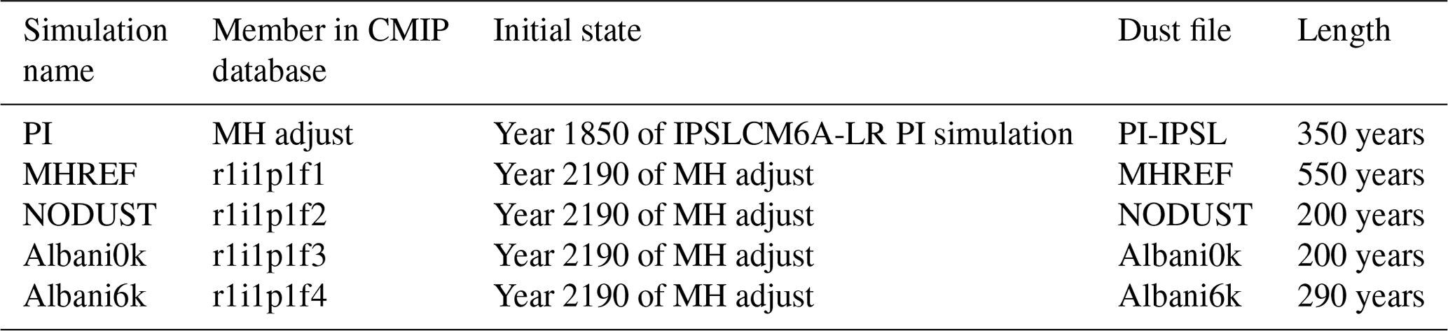
Table 1 Characteristics of the different experiments in terms of initial state, 3D dust distribution and simulation length. Albani6k is 290 instead of 300 years long. The last 10 years should have been run on a new computer with the risk to obtain non-continuous results due to the new running environment of the new computer. The second column indicates the experiment member posted on the ESGF CMIP6 database.

The initial state for the mid-Holocene simulation is the year 1850 (1 January) of the CMIP6 reference pre-industrial simulation with the same model version (Boucher et al., 2020). The same initial state was used for one of the members of the IPSL CMIP6 historical simulation. The Earth's orbital parameters and the atmospheric composition were switched to the values provided by Otto-Bliesner et al. (2017) for the mid-Holocene (Table 1). This mid-Holocene simulation follows exactly the PMIP4-CMIP6 protocol for the mid-Holocene. A tiny difference with the estimation of the forcing provided in Otto-Bliesner et al. (2017) is due to the fact that the pre-industrial control simulation does not have Earth's parameter values for 1850 but the ones for circa 1987 (Lurton et al., 2020). The solar constant is set to 1361.2 W m⁻².

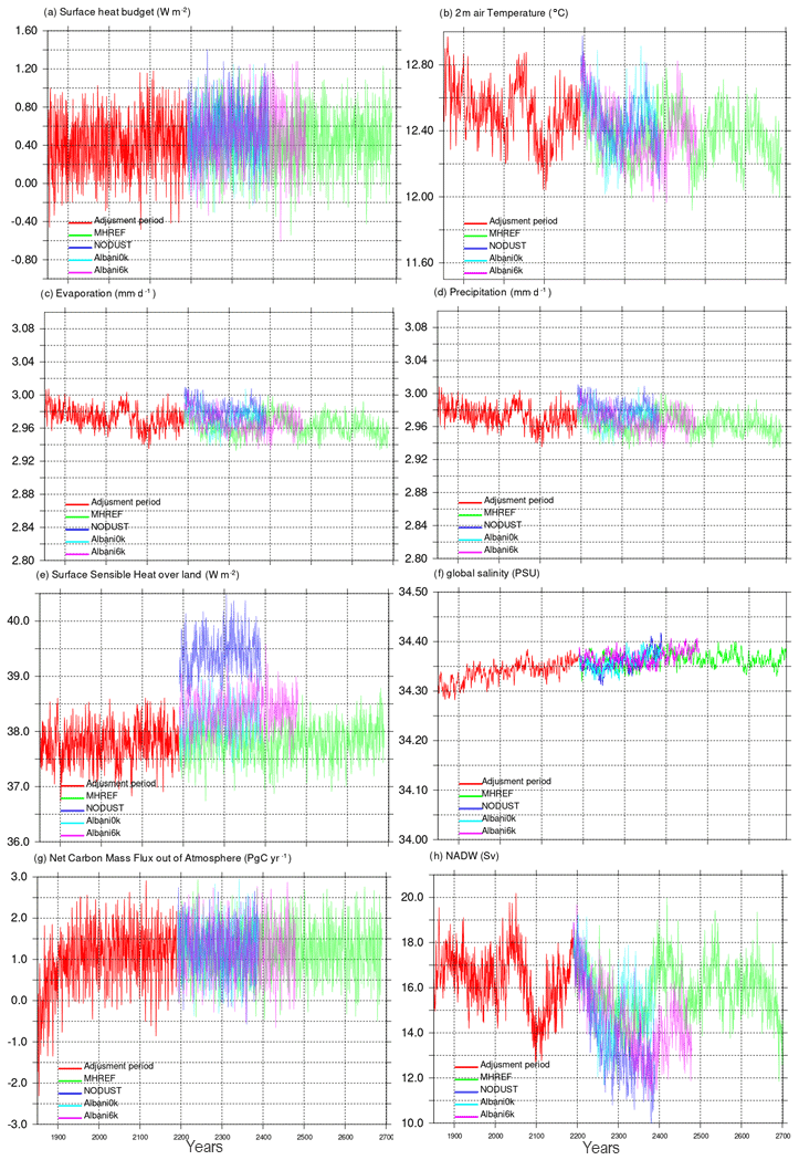
Figure 1 Temporal evolution of a subset of atmosphere, ocean and land surface variables for the different simulations: (a) surface heat budget (W m⁻²), (b) 2 m air temperature (^∘C), (c) evaporation (mm d⁻¹), (d) precipitation (mm d⁻¹), (e) surface sensible heat over land (W m⁻²), (f) global salinity (PSU), (g) net ecosystem productivity (Pg C yr⁻¹) and (h) maximum overturning in the North Atlantic (Sv). In each plot, the red curve represents the adjustment phase from the pre-industrial condition when the mid-Holocene forcing (Earth's orbit and trace gases) is switched on. The green curve corresponds to the reference mid-Holocene simulation (MHREF), whereas the other curves stand for the different sensitivity tests to dust forcing, starting from the same initial state as the reference mid-Holocene (MHREF) simulation (Table 1).

The model was then run for 350 years, which is long enough to bring the climate to equilibrium for mid-Holocene conditions (Fig. 1, red curve). However, we note that the carbon cycle is not fully equilibrated and manifests a small drift in the deep ocean (not shown). Most surface variables adjust in about 100 years. Note that the model produces large decadal variations (Fig. 1), which imposes to compute the mean annual cycle using at least 100 years. We chose 150 years in the following.

The last state of this simulation is used as initial state for the reference PMIP4-CMIP6 mid-Holocene simulation. This reference was run for 550 years, the last 50 years having high-frequency outputs for the analyses of extremes or to provide the boundary conditions for future regional simulations. This reference simulation is called CMIP6.PMIP.IPSL.IPSL-CM6A-LR.midHolocene.r1i1p1f1 in the ESGF database and MHREF in the text below (Table 1).

2.2 Pre-industrial and mid-Holocene dust fields for simulations with the IPSL model

The most striking feature of the Holocene dust cycle is the drastic reduction of dust emissions from today's major dust source, North Africa, compared to either late glacial, late Holocene or present levels (e.g. deMenocal et al., 2000; McGee et al., 2013; Palchan and Torfstein, 2019). Dust emissions were probably also lower in the Middle East (e.g. Pourmand et al., 2004), while more scattered signals emerge from East Asia (e.g. Kohfeld and Harrison, 2003). Dust emissions in the Southern Hemisphere were higher during the mid-Holocene than in the late Holocene, but much lower compared to the glacial period (Lambert et al., 2008). These and many more observational constraints were compiled at the global level, also accounting for the particle size range and distributions, and served as the basis for “data assimilation” in combination with the CESM model (Albani et al., 2015) to provide the PMIP4 reference field for the mid-Holocene (Otto-Bliesner et al., 2017).

Before being uplifted from source regions, dust particles consist of mineral aggregates of several hundred micrometres in diameter. Through bombardment, mineral aggregates are fractionated into smaller particles with diameters generally between 1 and 50 µm that can be transported over large distances of hundreds to thousands of kilometres. Each aerosol model has its own representation of these mineral dust particles. Adapting the original “Albani/CESM” PMIP4 datasets (Otto-Bliesner et al., 2017) for dust to the IPSL model thus required adapting the size distribution from a sectional representation to a modal one. Hence, the amount and horizontal spatial variability of the original Albani/CESM PMIP4 datasets are very similar to the actual prescribed datasets used in this work, although they are not identical. Figure 2 provides a comparison of the interpolated reference dust fields (Albani0k and Albani6k) to the observational dataset used to constrain the original PMIP4 reference dust fields (Albani et al., 2015). In particular, the ratio in model dust loads is compared to the ratio in dust deposition (< 10 µm diameter) from the observation. It is possible to see clearly the $-/+/-$ pattern in dust loads over North Africa, West Asia and East Asia, associated with the dust load changes between the mid-Holocene and the pre-industrial climates. It highlights that most of the changes agree with observed changes, except in East Asia or North America where the degree of agreement is heterogeneous (Fig. 2). The CESM simulated dust fields were obtained using an “assimilation” process, so that the causes of Holocene variability cannot be inferred from the simulations themselves. For the Middle East and Central Asia region, the observational constraints that were used are on two marine sediments records from the Arabian Sea (Pourmand et al., 2004) and the GISP2 ice core record from Greenland (Mayewski et al., 1997), based on information on dust provenance (Bory et al., 2003). There is a scarcity of relevant data and significant uncertainty for this region. Extensive evaluation of these original simulated dust fields against observations is available in Albani et al. (2016, 2015).

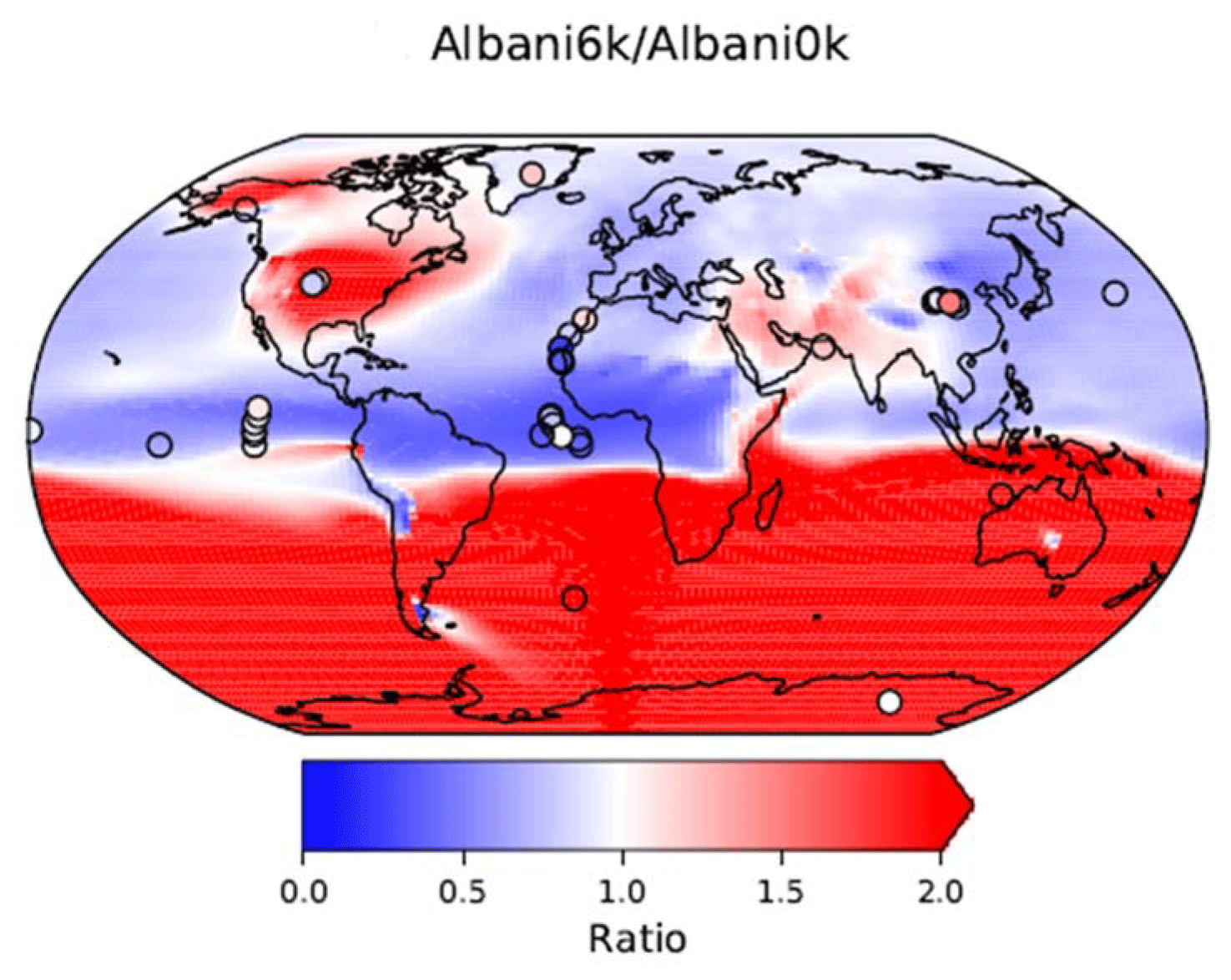
Figure 2 Ratio between Albani et al. (2015) mid-Holocene and pre-industrial dust loads (colour map) and ratio of dust deposition as estimated from dust reconstruction (coloured circles).

To obtain these files, we first had to transfer the information on the four bins provided in the 0.1–10 µm diameter range to the model size distribution of the target IPSL model [1 mode with mass median diameter (MMD) 2.5 µm and standard deviation (SD) 2.0]. The dust mass associated with the size distribution in the original dataset was remapped to the IPSL model aerosol scheme for each grid box in the 3D dust atmospheric concentration field. One implication of this procedure is that, compared to CESM simulations, the IPSL simulations have less dynamical variability of aerosol optical depth (AOD) and dust radiative effect (DRE) as a function of changes in size distributions with size. This is caused by the homogenisation needed for the dust interactions with radiation in the IPSL model due to the fixed optical properties of the single mode. In addition, the vertical discretisation of the original model consists of 26 vertical layers whereas there are 79 layers for the IPSL model. Therefore, the 3D dust concentration fields are interpolated in the vertical accordingly. Monthly fields of dust load and concentrations provided for PMIP4 and computed using the CAM model (Albani et al., 2015) were thus re-gridded from the resolution of CAM4 (horizontal 288 × 192 (1.25^∘ × 0.94^∘) with 26 layers in the vertical) to the IPSLCM6-LR resolution of 144 × 143 (2.5^∘ × 1.28^∘) and 79 vertical layers. When the mid-pressure of IPSLCM6 was delimited by two vertical levels from CAM4, the fields were interpolated between these two levels. If a mid-layer from IPSLCM6-LR was below (respectively above) the lowest (respectively highest) mid-layer of CAM4, we assigned to this layer the values of dust fields from the lowest (respectively highest) CAM4 level.

Table 2 Global budgets of simulated dust-related variables. Dust effective radiative perturbation (W m⁻²) is the globally averaged net (SW+LW) TOA effective radiative perturbation estimated from the first 50 years of the simulation and calculated as a difference compared to the NODUST simulation. It thus includes initial model adjustment as discussed in Albani and Mahowald (2019). The Dust absolute effective radiative perturbation (W m⁻²) is similar but considers the perturbation irrespective of the sign. The CESM1 PI and MH cases refer to the original simulations (Albani and Mahowald, 2019) that serve as the PMIP4 dust reference fields (Otto-Bliesner et al., 2017). This is the only table for which the comparison is done to NODUST, since it highlights the impact of dust in the climate system and not the effect of dust on the mid-Holocene climate, which is discussed in the main text of the paper.

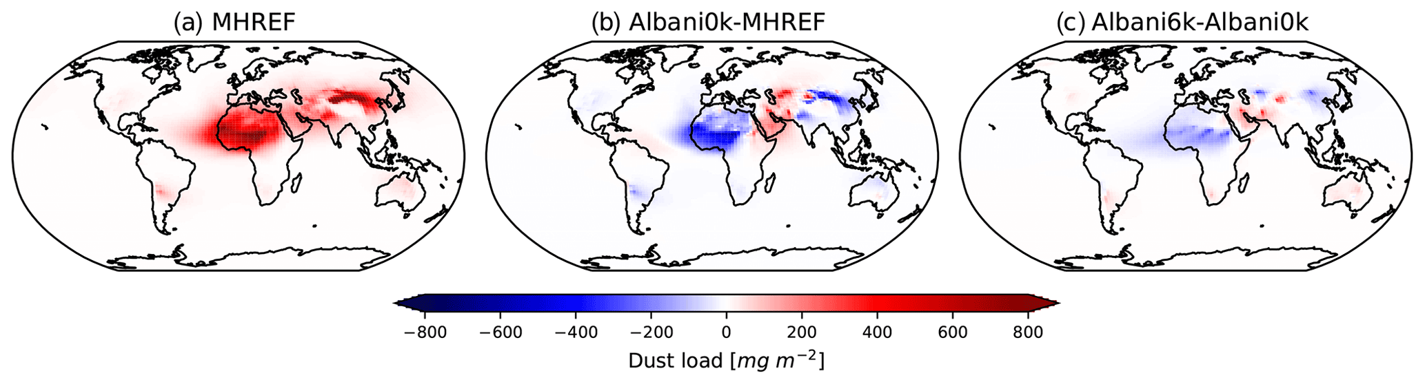
Figure 3 Comparison of the annual mean dust loads (mg m⁻²) from the different simulations. (a) Reference version with the present day IPSL dust load as used in the reference mid-Holocene simulation, MHREF. (b) Differences between Albani's and the IPSL PI dust load and (c) differences between Albani's MH and PI dust load.

The global dust load for the MHREF, Albani0k and Albani6k simulations is 18.7, 14.6 and 12.8 Tg respectively (Table 2). For comparison, the original dust loads for the Albani/CESM pre-industrial and mid-Holocene are 20 and 18 Tg respectively (Albani and Mahowald, 2019; Otto-Bliesner et al., 2017). Interestingly, the size distributions and optical properties of these Albani and Mahowald (2019) dust files interpolated on the IPSL model size distribution and spatial resolution are similar to the reference version of the IPSL model. Therefore, the dust load differences between IPSL model simulations reported in Table 2 are related to the 3D spatial distribution of dust (Fig. 3).

2.3 Dust sensitivity experiments

We performed three sensitivity experiments (Table 1) using the same model setup and initial state as the reference simulation MHREF. The first sensitivity experiment (referred to as NODUST below) allows us to study the extreme case in which no dust would be present in the mid-Holocene. This provides the largest change we can expect from dust forcing. This simulation of the CMIP6 database is the mid-Holocene member r1i1p1f2 (Table 1). In this simulation the dust load and the 3D dust distribution are set to 0. All other aerosols are kept as in the mid-Holocene reference simulation. We then examine the effect of having mid-Holocene dust instead of pre-industrial dust in the mid-Holocene simulations using Albani's mid-Holocene dust fields presented in Sect. 2.2. However, the 3D distribution of Albani's pre-industrial dust field is different from the IPSL one. In particular MHREF has higher dust loads over North Africa, the Thar desert and East Asia, whereas Albani0k and Albani6k have higher dust loads than MHREF in the Middle East and Central Asia (Fig. 3). Therefore, the differences in the pre-industrial dust distribution need to be considered in the analyses because they also affect the Albani's mid-Holocene dust distribution (Fig. 3, Table 2). We thus performed two simulations. The Albani0ksimulation (r1i1p1f3 in CMIP6 database, Table 1) tests the effect of replacing the IPSL dust fields by Albani's dust fields obtained for the pre-industrial climate. The last simulation, Albani6k (r1i1p1f4, Table 1), is run with Albani's dust fields obtained for the mid-Holocene and tests the effect of mid-Holocene dust when compared to Albani0k. We named the experiments NODUST, Albani0k and Albani6k, as this has the advantage of making a direct link with the corresponding dust files (Table 1). The NODUST and Albani0k sensitivity experiments were run only for 200 years and Albani6k for 290 years (Table 1).

Since dust forcing is small when globally averaged, these simulations equilibrate rapidly to the forcing induced by the replacement of a dust distribution by another and are quite stable (Fig. 1). Indeed, the globally averaged net (SW+LW) TOA dust effective radiative perturbation is in the range of −0.11 to −0.07 W m⁻², with larger negative radiative perturbation for pre-industrial dust as expected (Table 2). We call this measure effective perturbation (ERP) and not effective radiative forcing (ERF) as in Forster et al. (2016), because it is estimated by comparing each simulation with a simulation in which dust is suppressed (i.e. NODUST here) over the first 50 years of the simulation. It thus includes dust forcing and fast adjustment feedbacks. These radiative perturbations are small but slightly higher than in the original CESM1 simulations for which it is −0.06 and −0.03 W m⁻² for PI and MH respectively (Albani and Mahowald, 2019). The comparison of the sum of absolute values of dust ERP at each grid point provides higher values by avoiding compensation between regions of negative and positive dust ERP. It ranges between $\left|\mathrm{0.56}\right|$ and $\left|\mathrm{0.80}\right|$ W m⁻² in the IPSL model against $\left|\mathrm{0.27}\right|$ and $\left|\mathrm{0.23}\right|$ W m⁻² in CESM, indicating stronger geographical gradients in the IPSL model response (Table 2). This comparison indicates that the interpolation of the Albani et al. (2015) dust file on the IPSL model leads to a slight reduction of dust load. It also highlights that differences between other factors such as the radiative effect are not necessarily consistent with the dust load. Differences between the simulations discussed here and the original estimates by Albani and Mahowald (2019) presented in Table 2 can be interpreted as due to other differences in the treatment of dust between the two models (size distributions, optical properties, vertical distributions) as well as to non-dust-related (radiative transfer, boundary layer, etc.) processes and parameterisations.

The mean annual cycle discussed for these estimates and below refers to averages over 150 years. To avoid any artificial differences due to possible long-term adjustment and to the large centennial variability seen for example for the 2 m air temperature (Fig. 1b) or the North Atlantic Deep Water (NADW) (Fig. 1h), the mean seasonal cycle for the reference simulation (MHREF) is computed over the same period. It corresponds to the period between year 2250 and 2400 in Fig. 1 (i.e. year 50 to 200 of the mid-Holocene simulations stored on ESGF). During this common period all simulations have a similar long-term variability (Fig. 1). In the following we use the longer MHREF simulation to estimate the uncertainties resulting from variability. We also do not correct the different variables from the calendar effect when considering monthly averages (Bartlein and Shafer, 2019; Joussaume and Braconnot, 1997) because the effect is small for the mid-Holocene and corrections from monthly values do not allow us to keep the internal energy consistent between the variables, which is a critical aspect for this study. In order to avoid artificial calendar biases, we also consider January–February and July–August averages that correspond to peak seasons, whatever the period, to discuss seasonal differences.

3 Model adjustment and characteristics of the mid-Holocene climate

3.1 Adjustment to the mid-Holocene orbital and trace gases forcing

The dust experiments are designed to test the impact of dust on the mid-Holocene climate. We thus first discuss the differences between the mid-Holocene and the pre-industrial. The mid-Holocene changes in obliquity and precession have an impact on the seasonal spatio-temporal distribution of insolation, but not on its global annual mean. The rapid adjustments seen on most variables plotted in Fig. 1 between year 1850 and 1950 are thus primarily due to the model adjustment to the reduced trace gases (Brierley et al., 2020; Otto-Bliesner et al., 2017). They correspond to a reduction (about 0.4 ^∘C) in 2 m annual mean temperature (Fig. 1b). The temperature decrease induced by changes in insolation and trace gases is amplified by a slight increase in land albedo and an increase sea-ice thickness in the Southern Hemisphere (not shown). It is also compensated by a slight reduction in surface evaporation (Fig. 1c), which contributes to reduce the total precipitation amount (Fig. 1d). The reduced CO₂ and temperature lead to a global reduction of the total biomass (not shown) despite an increased carbon flux out of the atmosphere due to biomass productivity (Fig. 1g).

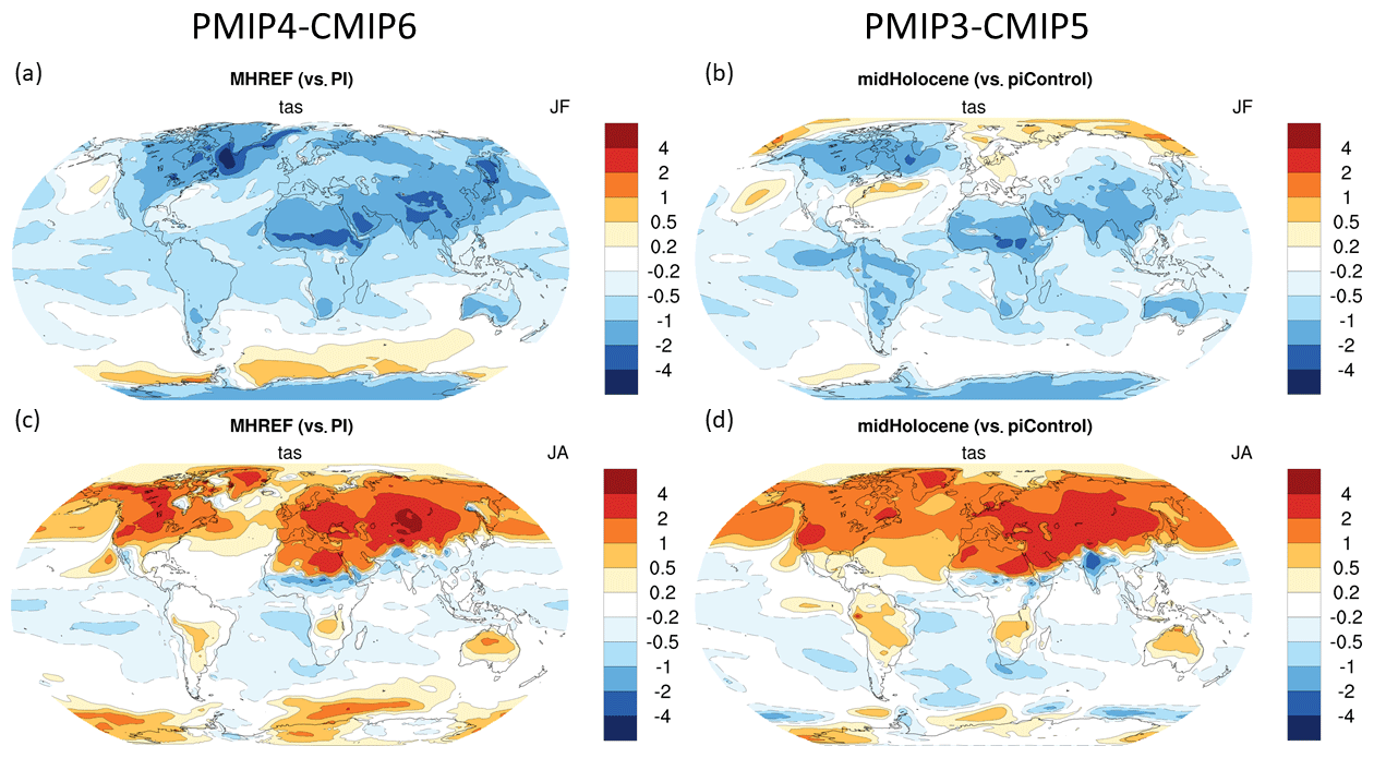
Figure 4 (a, b) 2 m air temperature differences (tas, ^∘C) between the mid-Holocene and the pre-industrial climates as simulated for January–February (JF) and (c, d) July–August (JA) in (a, c) the IPSL-CM61-LR PMIP4-CMIP6 simulations and (b, d) the IPSL-CM5A-LR PMIP3-CMIP5 simulations.

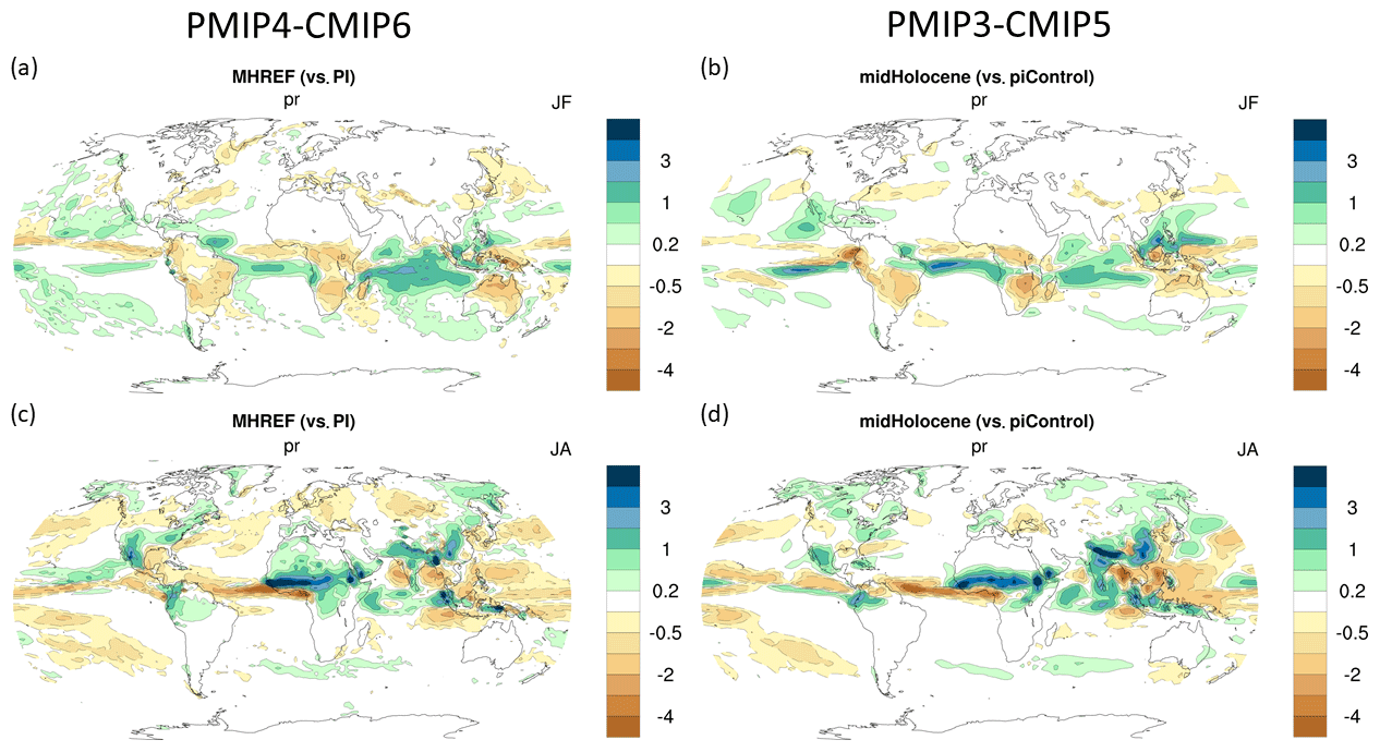
Figure 5 Same as Fig. 4 but for precipitation (pr, mm d⁻¹).

These annual mean changes are however small compared to the large seasonal variations induced by precession that enhance seasonality in the Northern Hemisphere and reduce it in the Southern Hemisphere. The model reproduces the well-known patterns of the simulated mid-Holocene climate (Figs. 4 and 5) (e.g. Braconnot et al., 2007). The reduced January–February (JF) insolation induces a general cooling over land, with a maximum in the subtropics and at the sea-ice margin. It also induces a tropical ocean cooling (Fig. 4a and b). These effects cause a strengthening of the Northern Hemisphere winter monsoon, leading to a drying over land and to wetter conditions over the ocean, in particular in the Indian Ocean (Fig. 4a and b). They also produce a slight southward shift of the intertropical convergence zone (ITCZ) in the Pacific and in the Atlantic (Fig. 5a and b). During mid-Holocene late spring, the increased solar radiation in the Northern Hemisphere, when the tropical ocean is still colder than today, enhances the interhemispheric and land sea contrasts, favouring the inland advection of moisture from the ocean onto the continent. Monsoon precipitations are enhanced and extend further north during July–August (JA), whereas precipitation is depleted over the ocean (Fig. 5c and d).

Compared to the PMIP3-CMIP5 IPSL-CM5A-LR simulation (Kageyama et al., 2013a), the PMIP4-CMIP6 IPSL-CM6-LR simulation produces a larger seasonal response in the Northern Hemisphere. It is mainly the result of colder winter conditions, which are also characterised by the fact that there is a JF mean cooling in the Arctic instead of the warming due to reduced sea-ice extent in the PMIP3-CMIP5 simulation (Fig. 4a and b). Part of this offset between the two simulations results from the changes in trace gases in PMIP4-CMIP6 that contribute to a global annual mean cooling of all PMIP4 simulations (Brierley et al., 2020; Otto-Bliesner et al., 2017). The other part is attributed to regional differences between the two model versions as discussed in Boucher et al. (2020). Several important differences also appear in JF in Eurasia over the GIN (Greenland, Iceland, Norwegian) seas and over the Arctic (Figs. 4a and b, and 5a and b). The JA monsoon precipitation is more intense and in better agreement with data reconstructions from West Africa. It extends further to the northwest of India and Pakistan.

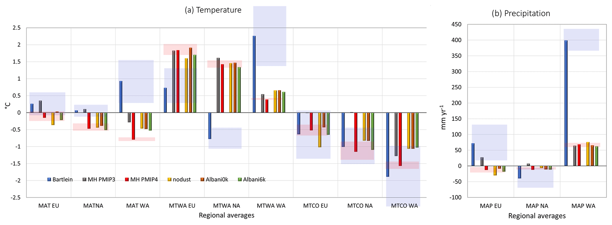
Figure 6 Comparison of the mid-Holocene simulated changes with Bartlein et al. (2011) temperature and precipitation reconstructions over Europe (EU), North America (NA) and West Africa (WA). The different indicators in (a) are the mean annual temperature (MAT, ^∘C), the temperature of the warmest month (MTWA) and the temperature of the coldest month (MTCO, ^∘C), and in (b) the mean annual precipitation (MAP, mm yr⁻¹). The blue intervals stand for the reconstruction uncertainties, estimated from the standard deviation provided by Bartlein et al. (2011) for each grid point. The red intervals stand for the mean root mean square difference between non-overlapping 150 year averages computed from the MHREF simulation and used here as an estimate of model mean annual cycle uncertainty.

Figure 6 summarises that the differences in North America, Europe and West Africa between the two model versions (grey and red bars in Fig. 6) are significant and larger than the mean differences between 100-year periods arising from internal variability (red intervals in Fig. 6). The larger cooling in MHREF (MH PMIP4) compared to MH PMIP3 leads to a better agreement with Bartlein et al. (2011) reconstructions of the coldest month temperature over the three regions (Fig. 6a). There are little changes in the representation of the warmest month. Because of this, the agreement for the annual mean temperature is poor for MHREF and even on the opposite sign compared to the reconstructions (Fig. 6a). Despite a change of sign in each of the region compared to MH PMIP3, the balance of the annual mean precipitation changes (MAP) between western North America and Europe is still incorrect in MHREF. Also, the increase JA African monsoon precipitation (Fig. 5) and the improvement of model climatology of PI and of the historical climate over west Africa (Boucher et al., 2020) are not sufficient to match the reconstructed precipitation over West Africa (Fig. 6b). This partly comes from the size of the regions that do not necessarily allow us to detect the increased precipitation in Sahel-Sahara that are compensated by less intense precipitation further south. Nevertheless, the magnitude of the simulated changes is too small, even when considering the large error bars from the reconstruction. This rapid overview indicates that the MHREF differences with the previous IPSL mid-Holocene reference simulations translates into little improvement in model skill when compared with palaeoclimate reconstructions at the regional scale as is further discussed by Brierley et al. (2020) for all available PMIP4-CMIP6 simulations.

3.2 Major differences between the dust sensitivity experiments

Changes induced by dust are of much smaller magnitude than the ones caused by insolation and trace gases (Fig. 7). The largest global radiative imbalance induced by dust forcing and fast feedback at the top of the atmosphere is found in NODUST and reaches about 0.1 W m⁻² compared to MHREF (Fig. 1). In other words, completely removing dust induces a positive dust ERP and a slight global warming, enhances global evaporation and global precipitation, and increases sensible heat flux over land compared to the other simulations. The effect of dust on the global model adjustment is smaller than the decadal fluctuations found for most variables (Fig. 1). This justifies that we estimate the 150-year mean annual cycle for the exact same period in all simulations with respect to their identical initial state.

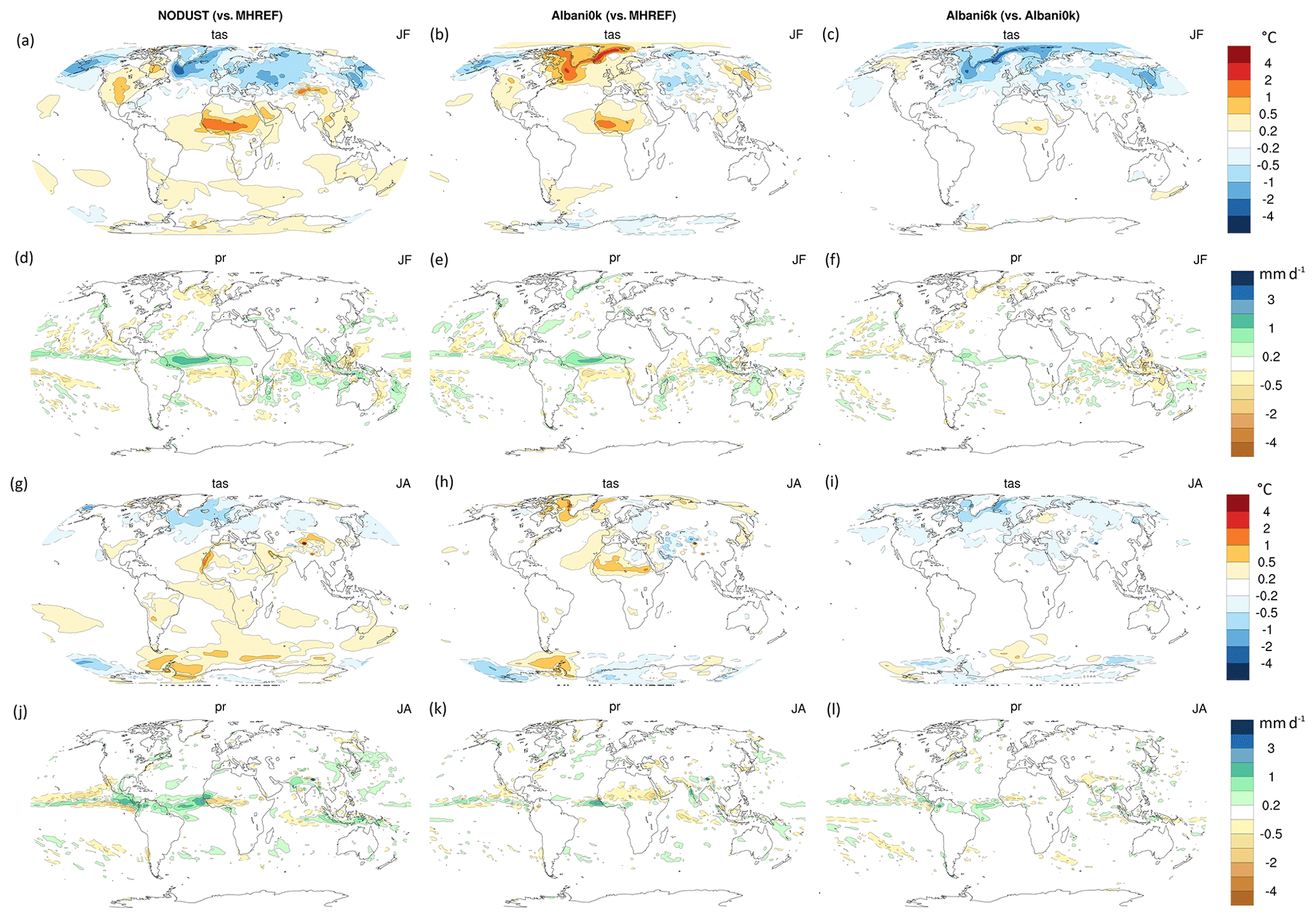
Figure 7 Impact of the different dust forcings on the simulated mid-Holocene climate for (a–e) mean January–February (JF) differences and (g–l) mean July–August (JA) differences. Panels (a), (b), (c), (g) and (i) represent the differences for temperature (tas, ^∘C) and (d), (e), (f), (j), (k) and (l) for precipitation (pr, mm d⁻¹). The first column highlights the effect of suppressing dust (NODUST–MHREF), the middle column the effect of replacing IPSL pre-industrial dust by Albani's pre-industrial dust (Albani0k–MHREF) and the last column the effect of mid-Holocene dust considering Albani's dust files (Albani6k–Albani0k). Note that for direct comparison with the magnitude of the differences induced by the insolation forcing, the legend is the same as in Figs. 4 and 5.

Suppressing dust causes a JF warming of up to 2 ^∘C in West Africa and over the Tibetan Plateau as more shortwave radiation reaches the surface (Fig. 7a). A slight cooling of about 1 ^∘C is also simulated in the North Atlantic and a warming at the margin of sea-ice in the Southern Hemisphere. These large-scale changes in temperature affect the large-scale hemispheric gradients and lead to an increase/decrease in precipitation in the northern/southern flank of the intertropical convergence zone (ITCZ) over the Atlantic and East Pacific oceans (Fig. 7d). During JA, surface warming is limited to the coastal regions in West Africa, the Tibetan Plateau and the Taklamakan and northern Chinese deserts (Fig. 7g). The African monsoon precipitation is increased at the coast and reduced inland, resulting in a slight increase when averaged over the African monsoon region (Fig. 6b). Precipitation is increased in North India and reduced over the tip of India (Fig. 7i). The largest precipitation differences with MHREF are found over the ocean where tropical Atlantic precipitation is increased and in the Pacific with a southward shift of the ITCZ.

Because of the much lower dust loads over North Africa in Albani0k compared with MHREF (Fig. 3b), the Albani0k–MHREF difference pattern (central column in Fig. 7) shares similarities with NODUST–MHREF over Africa, e.g. the JF surface warming over West Africa (in Fig. 7b and a), and precipitation changes in the tropical Atlantic, Africa and the Indian Ocean (Fig. 7e vs. d). A slight warming in the North Atlantic is simulated in both seasons (Fig. 7b and h). It is associated with a sea-ice reduction in the Labrador Sea. The drying of the African monsoon covers a broader area than in the NODUST case, and the rain belt is shifted southward in the Atlantic Ocean (Fig. 7k). The differences in the JA Indian monsoon (Fig. 7k vs. j) reflect the fact that dust loads in Albani0k are larger than in MHREF over the Arabian Sea or Indian Ocean and lower over the Indian subcontinent (Fig. 3).

The dust load is reduced in Albani6k compared to Albani0k (Fig. 2). However, since the reduction is achieved with a minus/plus pattern between Africa and India, the simulated climate changes are different from NODUST, for which dust is suppressed everywhere. As in NODUST, a cooling and drying expand from the North Atlantic to the Eurasian continent during JF (Fig. 7c). The cooling persists with a small magnitude during JA (Fig. 7i). Compared to NODUST-MHREF, a drying is simulated both for the African and the Indian monsoon regions, as well as a southward shift of the rain belt both in the Atlantic and the Pacific oceans (Fig. 7).

Over Europe, NODUST and Albani6ka, when respectively compared to MHREF and Albani0k, indicate that reducing dust leads to colder annual temperature minimum (MTCO) and colder annual temperature maximum (MTWA), with a larger magnitude than the centennial model variability (Fig. 6). Over North America the effect of dust pattern seems prominent. NODUST and Albani0k have common behaviour with a similar reduction of MTCO and no difference for MTWA compared to MHREF, whereas Albani6k produces MTCO cooling and reduced MTWA (Fig. 6). These differences are still in agreement with the reconstructions for MTCO and do not reduce the large model bias for MTWA or the annual mean (MAT). In West Africa, MTCO and MTWA in Fig. 6 reflect the regional warming discussed in Fig. 7. The associate reduction of precipitation over the continent is also not going in the right direction for improved representation of the regional climate change, even though the effect is small compared to the large discrepancy between the simulations and Bartlein et al. (2011) reconstructions.

Figure 8 Identification of the regions where differences are maximum between (a, c, e, g) the mid-Holocene dust sensitivity experiments compared to (b, d, f, h) regions where centennial variability is maximum. Panels (a), (b), (c) and (d) provide the results for 2 m air temperature and (e), (f), (g) and (h) for precipitation. The different analyses correspond to (a, e) mean root mean square differences between the four mid-Holocene simulations with different dust forcing, (b, f) mean root mean square differences between non-overlapping 100-year periods of the reference mid-Holocene simulation MHREF and (a, b, g, f) months for which the root mean squares for the different analyses is maximum. 2 m air temperature is expressed in ^∘C and precipitation in mm d⁻¹.

In order to identify the regions where the different sensitivity experiments exhibit the largest differences, we computed the root mean square difference between the four simulations over the whole annual mean cycle and highlighted the month for which the root mean square is at a peak. We compare these results to those computed for centennial variability, considering several non-overlapping 150-year mean annual cycles in the MHREF simulation. The results, shown in Fig. 8, indicate that the differences in the tropics over land for temperature (Fig. 8a and c) and over land and ocean for precipitation (Fig. 8e and g) are indeed fully induced by dust forcing, whereas in mid- and high latitudes the temperature pattern shares lots of similarities with centennial variability both in magnitude and peak month (Fig. 8b and d). For precipitation, variability is also large in the tropics, but with smaller magnitude and different peak months in most places than for the impact of dust forcing (Fig. 8f and h). Figure 8 confirms that the maximum impact of dust on temperature in the tropics is found in West Africa, south of Lake Chad, and over the Arabian Peninsula during boreal winter from November to February (i.e. either month 11–12 or 1–2), and north of Lake Chad in boreal summer in July–August (month 7 or 8). For precipitation, the impact of dust is maximum during the West African summer monsoon season, in contrast with variability that peaks in Autumn (Fig. 8g and h). Note that over the ocean peak differences between the effect of dust and variability share lots of similarities, except that larger and more homogeneous regions of similar peak differences are found for the dust signal (Fig. 8g). Maximum differences are mostly found during summer except in the west tropical Atlantic where the spring season certainly reflects a slight shift in the timing of the migration or in the location of the Atlantic rain belt.

3.3 Moist static energy and atmospheric heat transport

The seasonal differences shown in Fig. 7 counteract or amplify the mid-Holocene signal depending on regions. Mid-Holocene changes in atmospheric column moist static energy (MSE, Fig. 9) are consistent with the changes in temperature and precipitation, and provide a more integrated view on the large-scale redistribution of energy associated with the insolation forcing. The major reduction of mid-Holocene MSE induced by insolation during JF occurs in the Atlantic sector with maximum value over South America and Africa, whereas the major increase occurs over the Indian Ocean and the West Pacific. The associated changes in total heat transport thus have a land–ocean symmetry and an inter-basin asymmetry with increased MSE transport from the Indian Ocean to the Atlantic and Pacific and across the Pacific Ocean. The combination of reduced/increased meridional heat transport in the Atlantic/Pacific leads to a net reduction of atmospheric heat exported from the tropical region to higher latitudes in both hemispheres. It reaches about 0.18 PW at 40^∘ N and around 0.15 PW at 35^∘ S. During summer, the strong interhemispheric and land–sea differences induced by insolation and increased Afro-Asian monsoon enhance the energy export from the North Africa to the other ocean basins. This is mainly due to the large heating and specific humidity increase in this region. Note that the export from Amazonia is also increased. These changes induce a net southward difference in total meridional heat transport across the Equator that reaches about 0.3 PW.

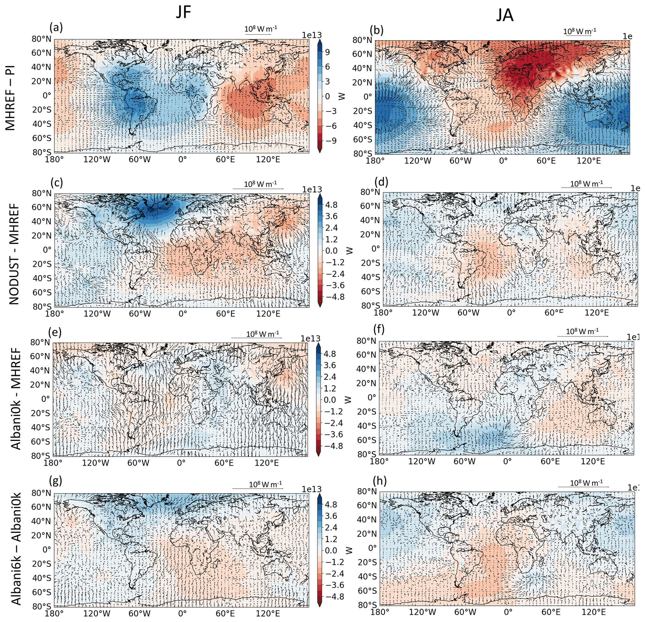
Figure 9 Difference of moist static energy integrated over the atmospheric column (W) and associated moist static energy transport (W m⁻¹) between (a) the January–February (JF) and (b) July–August (JA) averaged mid-Holocene reference and pre-industrial control simulations (MHREF–PI) , (c) the JF and (d) JA averaged mid-Holocene NODUST) and MHREF simulations (NODUST–MHREF), (e) the JF and (f) JA averaged mid-Holocene Alabani0k and MHREF simulations (Albani0o–MHREF), and (g) the JF and (h) JA averaged mid-Holocene Albani6k mid-Holocene Albani0k simulations (Albani6k–Albani0k). To better highlight the differences induced by the different dust fields a factor of about 2 has been applied to the legend and reference length of the arrow between the first row and the others rows.

As expected from the changes in temperature and precipitation shown in Fig. 7, the energetic changes induced by the different dust forcings are of lower magnitude (Fig. 9). However, both NODUST-MHREF and Albani6k-Albani0k are characterised by an increase in energy export from West Africa and South Atlantic subtropics to the North Atlantic in JF (Fig. 9b). This feature is strengthened over the SH subtropical Atlantic. The latter is consistent with a reduced influence of the Saint Helen anticyclone, which reduces the African monsoon (Figs. 4b and 5). Complete dust suppression in the NODUST-MHREF case therefore leads to a reinforcement of the insolation changes over the Asian sector and of the enhanced role of the Asian monsoon in the MSE export (Fig. 9b). It leads to an increase of the Equator-to-pole heat transport in each hemisphere that reaches about 0.1 PW at 35^∘ S, enhancing the role of the insolation forcing in the Southern Hemisphere and reducing it in the Northern Hemisphere. The situation is different with Albani6k because of the east/west dust load pattern over Asia, which counteracts the NODUST effect (Fig. 9d). Because of this, there is almost no impact on the Southern Hemisphere meridional atmospheric heat transport. The effect is similar to NODUST in the Northern Hemisphere because it is mainly driven by the Atlantic sector. The changes induced by Albani0k dusts reflect well the tripolar minus/plus/minus, dust load pattern between West Africa, the Middle East and East Asia (Fig. 3). During JF the reduced dust and the associated warming over Africa reinforce the energy export to higher latitudes as in the other two simulations. However, in this case, the atmosphere over the Indian Ocean becomes an energy sink. During JA, changes in the source and sink of atmospheric MSE counteract the effect of increased African monsoon while enhancing that of the East Asian monsoon (Fig. 9c).

These analyses reveal that even though the dust changes over Africa are large, the net impact on MSE sources and sinks over the West African region with maximum dust changes is small. The energetic response is driven by the changes in the Atlantic sector when dust is suppressed or reduced, and the role of East Africa in the global energetics is affected by the difference in dust pattern between Africa and Asia.

4 Global estimates and regional patterns of dust radiative forcing

4.1 Estimation of dust radiative forcing with two different methods

In Sect. 2.3, we estimated dust ERP in MHREF, Albani0k and Albani6ka in order to compare the dust radiative effect with those estimated by Albani and Mahowald (2019). We now go one step further by estimating the instantaneous dust forcing separately for SW and LW and considering MHREF as a reference, so as to identify the impact of dust reduction on the mid-Holocene climate (Table 3). We first diagnose the dust instantaneous radiative forcing (IRF) following the RFMIP protocol (Forster et al., 2016; Pincus et al., 2016). This is done by considering simulations with the atmosphere–land surface component of the coupled IPSLCM6-LR model used for the MHREF simulation and Sea Surface Temperature (SST) prescribed to pre-industrial conditions. We thus performed three 30-year-long simulations including a double call to the radiative scheme in order to diagnose the IRF associated with different dust fields, as done by Lurton et al. (2020) for historical and future climate. All simulations have mid-Holocene insolation and trace gases values. In a NODUST-type simulation with this model setup, we diagnose the impact of suppressing dust compared to the IPSL reference pre-industrial (IPSL-PI) dust field used in MHREF. In an Albani0k-type simulation, we diagnose the IRF of the Albani0k dust field with respect to the IPSL-PI reference dust field. Then in an Albani6k-type simulation the same procedure is applied to calculate the IRF of Albani6k dust field with respect to the Albani0k dust field. The results are averaged over the last 10 years of each run (Table 3). In all three simulations, the dust field used in the mainstream radiation call is reduced compared to the reference one (used in the second radiation call), so the annual global IRF-SW is positive, e.g. when dust is reduced or suppressed the Earth system receives more radiation.

Table 3 SW net and LW outgoing dust radiative forcing (W m⁻²) at TOA in clear sky and all sky conditions as estimated from the different simulations. The RFMIP-IRF method diagnoses the forcing online at each model radiation time step with respect to a reference (using a double call to the radiation scheme). This has been done here in simulations without oceanic adjustment. The Taylor et al. (2007) method diagnoses the total radiative forcing of dust (forcing and feedback) from the fully coupled experiment after ocean adjustment. This method does not allow us to diagnose LW IRF. The reader is referred to Sect. 4.1 and to the Appendix for details on the radiative forcing estimates.

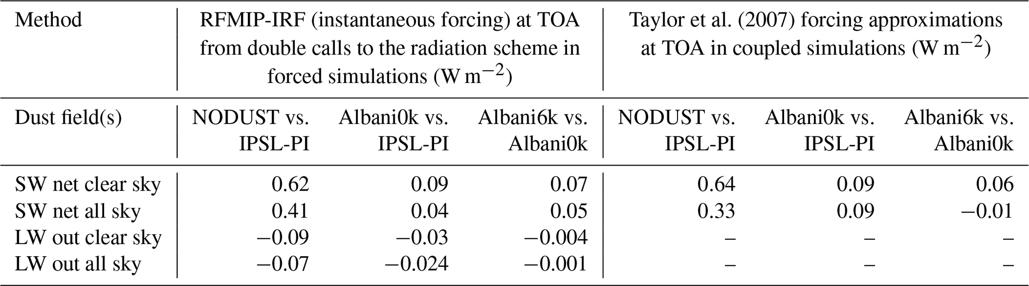
As expected, the annual global IRF-SW is maximum in the NODUST-type simulation, where the difference of dust conditions in the first vs. second radiation calls is maximum. IRF-SW reaches 0.62 W m⁻² in clear sky and 0.41 W m⁻² when clouds are also considered (Table 3). The effect of clouds partially offsets the direct effect of dust on albedo, which is mainly due to feedbacks from climate adjustment. The Albani0k IRF-SW, with respect to the same reference IPSL-PI, is much smaller: 0.09 W m⁻² in clear sky vs. 0.04 W m⁻² in all sky. Since the Albani0k total dust load (14.6 Tg) is only ∼ 20 % smaller than the IPSL-PI dust load (18.7 Tg) and these cases essentially share the same size distributions and optical properties, the differences mainly arise from the different horizontal dust patterns and altitude of dust in the atmosphere. Reduced mid-Holocene Albani6k dust load (12.8 Tg) compared to Albani0k results in an IRF-SW of the same order of magnitude as that of Albani0k vs. IPSL-PI, in both clear- and all-sky conditions. The IRF-LW is of smaller magnitude and is negative, which also partially offset IRF-SW. As for IRF-SW the interaction with clouds slightly damps the clear sky effect. Interestingly the IRF longwave is very small when comparing Albani6ka with Albani0k, compared to the two other cases. Also, the ratio with IRF-SW is larger for Albani0k. It stresses that the 3D-distribution in the atmospheric column and the spatial distribution are 2 key factors for this effect. In particular, the difference in dust altitude between albani0k and Albani 6ka is small compared to the other cases.

In order to estimate dust forcing and dust feedbacks in the adjusted coupled experiments, we also apply the simplified partial derivative method developed by Taylor et al. (2007), which is valid for shortwave radiation (see method description in the Appendix). In this method, the absorption and scattering properties of an equivalent atmosphere are computed from the radiative fluxes and the surface albedo. It allows for estimating changes in these atmospheric and surface properties on the planetary albedo and thereby on the net shortwave radiation at the top of the atmosphere. The comparison of the estimates using clear sky instead of all sky radiation variables provides an estimate of the direct effect of dust, whereas the difference between the clear sky and the all sky estimates provides an estimate of cloud feedback that reflects both the dust semi-direct effect and climate feedback.

The numbers obtained for clear sky with this method are quite close to the IRF-SW estimates (Table 3), indicating that dust radiative perturbation is dominant under clear-sky conditions and that interactions with clouds damp the total dust forcing (all sky). The estimates for all sky are however different (except for NODUST) suggesting that cloud distribution is different in the coupled simulations with SST adjustments. It however indicates that there is little impact of ocean feedbacks when moving from estimates in atmosphere alone simulations with prescribed modern SSTs to fully coupled mid-Holocene simulations for clear sky. It also provides an indirect evaluation of the Taylor et al. (2007) simplified method that proves to be rather accurate to estimate dust radiative effects.

4.2 Regional differences in dust radiative forcing and feedbacks

As expected from the different dust load maps (Fig. 3), the small global numbers of Table 2 mask larger regional values and the differences in radiative pattern changes induced by the different dust fields (Fig. 9a and b). The dust loads in the atmosphere have a seasonal distribution resulting from regional meteorology (winds), soil moisture and vegetation characteristics (Marticorena, 2014; Shao et al., 2011; Tegen et al., 2002; Zender et al., 2003). We only consider the SW clear sky forcing for illustration in Fig. 10, since this term is dominating dust forcing (Table 3). The comparison between IRF and the Taylor et al. (2007) clear sky estimates confirm that both global and regional estimates are similar (see Fig. A1 in Appendix). The increase in surface radiation in regions where dust is suppressed or reduced (Fig. 10) is directly the fingerprint of the reduced effect of the shadow effect of dust on incoming solar radiation at the surface. It follows the seasonal differences in dust loads quite well. As anticipated, there is a pattern of plus and minus values when considering Albani0k or Albani6k dust fields, characterised by increased dust loads along latitudes from East Africa to the Middle East (Fig. 2).

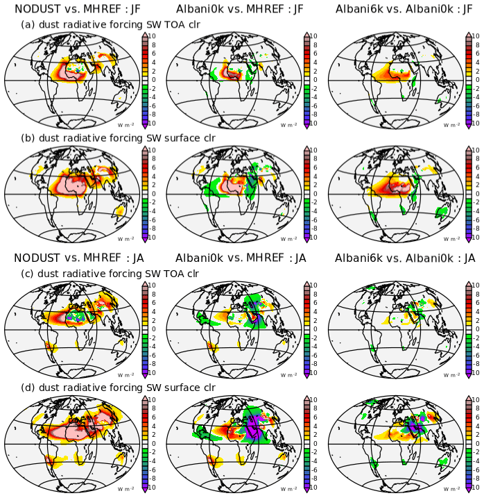
Figure 10 Comparisons of the radiative forcing (W m⁻²) induced by the different dust fields at (a, c) the top of the atmosphere (TOA) and (b, d) the surface for (a, b) January–February (JF) and (c, d) July–August (JA) averages. The radiative forcing has been estimated from online atmosphere alone simulations following the RFMIP protocol (see text). The left and middle columns represent respectively the difference between the NODUST (left) and Alanani0k (middle) estimates compared to the Mid-Holocene reference simulations (MHREF), and the right column represents the difference between the Albani6k and the Albani0k estimates. All fields are positive down to directly reflect the radiative budget at TOA or at the surface.

At the top of the atmosphere over the Sahel-Sahara region, the radiative effect of dust is a patchy SW pattern between the Sahara and the Sahel regions, whereas the differences in surface radiation more directly represent the minus/plus pattern of the differences in dust load (Fig. 10). Further exploration using the Taylor et al. (2007) methods indicate that the compensation at TOA over the Sahara comes from the compensation between the absorption and scattering effect of dust in the atmospheric column (Fig. 11). It leads to almost no changes in SW radiation at TOA over the Sahel-Sahara region during JF and reduced radiation in JA. This is consistent with previous results obtained with the aerosol models INCA (Balkanski et al., 2007) and CESM1 (Albani et al., 2014), and in agreement with satellite-based estimates (Patadia et al., 2009) averaged over Sahara for present day. These studies highlight that the response over the Sahara is due to dust SW direct radiative effect and that it depends on the albedo of the underlying surface (Albani and Mahowald, 2019; Patadia et al., 2009). The impact is not a direct effect of the surface albedo (not shown) but the effect of dust absorption and thereby of the relative balance between the changes in dust absorption and scattering that is affected by the surface condition (brightness).

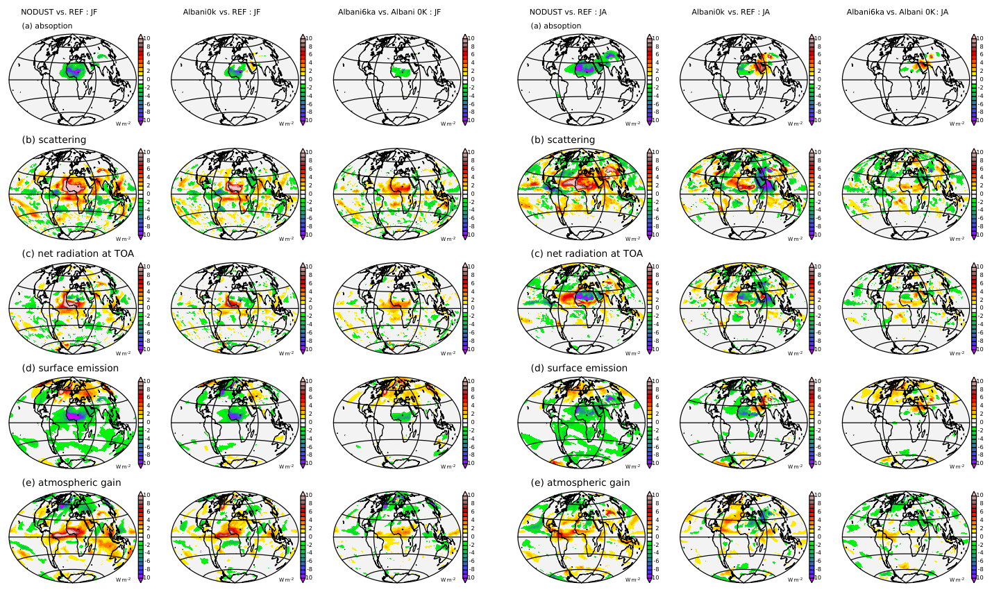
Figure 11 Impact of dust on top of the atmosphere radiation considering the decomposition of Taylor et al. (2007) for shortwave radiation. The first part of the figure refers to January–February averages and the second part to July–August averages. (a) The effect of changes in atmospheric absorption, (b) the effect of atmospheric scattering and (c) the change in net radiation (SW+LW) at the top of the atmosphere (TOA), and for longwave the estimate of (d) the change in surface emission due to temperature (Planck emission) and (e) the effect of changes in the atmospheric heat gain, which represent the aggregated effect of changes in atmospheric lapse rate, change in atmospheric water vapour and changes in clouds. From left to right the different panels show the results for the NODUST, the Albani0k and the Albani6k simulations, with reference to MHREF for NODUST and Albani0k and reference to Albani0k for Albani6k. All terms are positive downward to directly reflect the relative impact of each of these terms on the atmospheric radiative budget et the top of the atmosphere. The change in net radiation at TOA is also the sum of all the other terms, given that the effect of changes in surface albedo due to changes in leaf area index is negligible (not shown).

In the regions directly affected by the change in dust, the shortwave radiations in Fig. 10 are very similar to values found for clear sky conditions and reflect the direct impact of dust on the atmospheric radiative forcing (Fig. 10). Outside these domains, the values estimated with the Taylor et al. (2007) method reflect the feedbacks by atmospheric clouds induced by the changes in the atmospheric circulation and in sea-surface temperature and sea-ice cover (Fig. 11). In all three simulations, changes induced by the seasonal evolution of vegetation Leaf Area Index (LAI) are small (not shown), but the albedo effect diagnosed on TOA radiation indicates it has a small impact on the simulated climate in Southern Europe and northern tropics in JF and over a small band in Sahel in JA, reflecting less active vegetation where monsoon is reduced in this simulation. Figure 10 and 11 confirm that the largest TOA forcing and feedbacks are found in the Atlantic sector in JF for all cases and that in JA they extend from Africa to Asia (Chinese deserts) in NODUST compared to MHREF. The increase in net radiation in the Atlantic sector is compensated by a decrease in East Africa in Albani0k. The changes in SW radiation are of smaller magnitude in Albani6k when compared to Albani0k and reflect a mixture of the NODUST case and Albani0k case forcing and feedback estimates with MHREF as a reference.

The Taylor et al. (2007) method cannot be applied to longwave radiation. For longwave we provide an estimate of the global impact of dust forcing and associated feedbacks by estimating, on one hand, the surface emission using the Planck function and surface temperature and, on the other hand, the total atmospheric heat gain from the difference between outgoing radiation and surface emission. As expected, regions with strong shortwave radiative effects induced by dust are associated with a surface warming and emit more radiation out of the atmosphere. This effect is partially compensated by lapse rate, humidity and cloud feedbacks, as well as the dust effect on LW in the atmospheric column (Fig. 11). These analyses stress that the amount of dust alone is not sufficient to explain mid-Holocene dust forcing, but that the geographical distribution of the forcing is also very large and varies substantially from one dust model to another, inducing substantial differences between Africa and India.

5 Analyses of the impact of the different dust forcing on the Afro-Asian monsoon and Atlantic overturning

5.1 The African and Indian monsoon responses to insolation forcing

We now discuss in more detail the altitude versus latitude profiles over West Africa and India to show how dust affects atmospheric convection and precipitation, and how the dust effect acts on the insolation forcing (Figs. 10 and 11).

Figure 12 Zonal averages of the July–August (JA) mean atmospheric circulation over the (a–d) West African (10^∘ W to 10^∘ E) and (e–h)  Indian (70 to 90^∘ E) monsoon regions showing the effect of (a, e) the mid-Holocene insolation compared to the pre-industrial climate (MHREF–PI), (b, f) the effect of NODUST on the mid-Holocene climate (NODUST–MHREF), (c, g) the effect for Albani0k on the mid-Holocene climate (Albani0k–Albani6k) and (d, g) the effect of Albani6k compared to Albani0k on the mid-Holocene climate (Albani6k–Albani0k). Each plot considers the atmospheric temperature (^∘C, colour scale), the meridional winds (with a −1 factor imposed on the vertical component in hPa/s to have more intuitive vision of upward and downward motions), the specific humidity (kg kg⁻¹, light and dark blue contours respectively for negative and positive value) and the dust concentrations (black contours, plotted on top of light grey where the dust content is reduced and dark grey where dust content is increased). For each monsoon region the top right panel has different scales, which reflect the larger impact of the insolation forcing and no dust contour, which accounts for the fact that there is no change in dust between the mid-Holocene reference simulation and the pre-industrial simulation.

When comparing the MH and PI PMIP4 reference simulations, we see that, in response to the JA insolation forcing, the temperature gradient is increased in the atmosphere at all levels over West Africa north of 20^∘ N and over India over the Tibetan plateau (Fig. 12). Between 10 and 20^∘ N in Africa and 25 and 35^∘ N in India, temperature changes have a barocline structure, with colder temperatures below 700 hPa and higher temperatures above, which coincides with the regions with maximum change in monsoon precipitation. It is located to the south of the maximum increase in low-level atmospheric moisture content in Africa and above it in India. In India the monsoon system is constrained by the Himalayan orography and these changes are located just at its foothills. In both regions, this pattern reflects the northward shift (or extent) of the monsoon rain belt and is associated with a local reinforcement of the southern branch of the Hadley cell that contributes to export heat from the monsoon system to the south (Figs. 12a and 9b). Further south, the temperature is reduced over the whole atmosphere. The increased atmospheric moisture content extends further north and is not limited to the rain belt regions. The moisture content increase also acts to set up the large-scale change in the atmospheric circulation (Fig. 9b). The fact that moisture increases total atmosphere MSE far north on the continent is an important aspect in the northward shift of the rain belt during the mid-Holocene. The changes in the atmospheric circulation are also characterised by a depletion of the atmospheric moisture content where subsidence is increased in the descending branch over the Atlantic Ocean south of 5^∘ N. Another difference between the African and Indian regions reflects the regional orography context. The maximum vertical velocity and precipitation is located to the south of the minimum temperature in Africa, whereas it is located over the minimum temperature in India. Figure 13a further highlights the mean changes between 10 and 20^∘ N. This box has been chosen so as to show the barocline atmospheric structure in temperature and zonal wind changes with increased inland monsoon flow from the Atlantic near the surface, the increase and upward shift of the 700 hPa African easterly jet (AEJ) and increase of the 200 hPa easterly jet at upper levels. The changes in the AEJ are associated with the changes in meridional temperature gradient in the middle atmosphere as discussed in Texier et al. (2000). Figure 13a also highlights the complex connection with the Indian monsoon in East Africa and over the Arabian Sea. The mid-Holocene is characterised by an increased alimentation of the AEJ from above and an increased subsidence over the Arabian Sea, where the subsiding flow joins the Indian monsoon southwest surface flow around 60^∘ E.

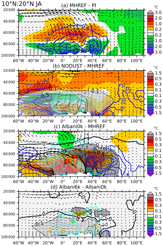
Figure 13 As in Fig. 12, but for the atmospheric meridional circulation averaged from 10 to 20^∘ N. These changes reflect the changes at the northern edge of the boreal summer monsoon rain belt in Africa for (a) MHREF-PI, (b) NODUST–MHREF, (c) Albani0k–MHREF and (d) Albani6k–Albani0k.

5.2 Role of dust on the mid-Holocene representation of the African and Indian monsoons

The suppression of dust has an impact from the surface to about 500 hPa in both regions, with the maximum impact north of 10^∘ N in Africa and north of 22^∘ N in India. The suppression of dust coincides with a slight reduction of atmospheric moisture content over Africa (Fig. 12b) and thereby a reduction of the large-scale meridional MSE potential (Fig. 9d). Over India, moisture is depleted over the tip of India but increased over the foothills of the Himalayas where upward motions and precipitation increase (Figs. 12f and 7k). Changes in the atmospheric column for temperature partially counteract the effect of insolation with warmer temperatures to the south and colder temperatures to the north. Differences in the atmospheric profiles between the insolation and dust forcing emerge in the regions where precipitation changes the most (Fig. 12). The solar forcing acts at the surface whereas the suppression of dust acts both at the surface, by allowing more radiation to reach the surface, and in the atmospheric column, by changing the local absorption and scattering properties. Different mechanisms are thus implied to increase/decrease the monsoon strength. Insolation induces surface feedbacks that first impact the large-scale gradients, large-scale dynamics and thereby moisture advection, which in turn is reinforced by local recycling (D'Agostino et al., 2019; Marzin and Braconnot, 2009; Zheng and Braconnot, 2013). Dust affects the surface temperature but also the temperature profile, relative humidity and atmospheric convection in the atmosphere, which in turn affects the large-scale circulation and the monsoon response. The results for Africa when dust is suppressed are consistent with previous findings on the role of dust. It was shown that the presence of dust reinforces the Saharan heat low in JA with enhanced monsoonal flow and atmospheric humidity, and that the spatial structure of precipitation anomalies induced by dust shows an increase in monsoonal precipitations over the Sahel only, which can be explained by the barocline structure of the atmosphere that facilitates convection there rather than further inland (i.e. Miller et al., 2014). The reverse is true with our dust reduction point of view. Over India, this effect is counteracted by the increased warming of the southern flank of the Himalayas that acts as a local elevated heat source in the atmosphere and triggers upward flow and increase moisture convergence (Fig. 12f). Therefore, the MSE energy source is increased over the Asian continent and reduced over Africa, enhancing the asymmetry between the two monsoon responses. Differences between the insolation and the NODUST-MHREF case also appear clearly when looking at the zonal atmospheric circulation (Fig. 13a). Over West Africa, the weakening of the low-level monsoon circulation is associated with a warming, except between 800 and 600 hPa, where a cooling is related to a downward shift of the AEJ. The AEJ is however reduced in the above layers. There is also increased inflow in East Africa from the subtropical jet. The connection between the African and Indian systems over the Arabian Sea sector is effective in the middle atmosphere but not at the surface. The latter correspond to the subsidence induced by increased precipitation over India and the Bay of Bengal (Figs. 7 and 8).

The zonal mean patterns in temperature, humidity and wind changes induced by the Albani0k dust on the MH climate or when comparing the effect of Albani6ka with Albani0k share similarities, with smaller magnitudes compared to the NODUST case over West Africa below 600 hPa (Fig. 12c and d). However, the surface warming extends further north and there is a clear barotropic structure with warmer temperatures between the surface and 600 hPa and colder above. The situation is different for India because of the zonal mean plus, minus, plus pattern in atmospheric dust load (Figs. 2 and 3). In Albani0k, the reduced dust over the Himalayan foothills compared to MHREF favours the local increase of monsoon precipitation there (Fig. 12g), whereas the relative increase in dust over the Indian Ocean and the Middle East (Fig. 2c) acts to decrease the MSE potential and the monsoon inland flow over East Africa, with a larger magnitude than in the NODUST case (Fig. 9). When Albani6k dust is considered instead of Albani0k, mid-Holocene dust is increased over India and the Tibetan plateau, which reduces the monsoon strength and the role of the heating source of the southern flank of the Himalayas (Fig. 12h). The 10–20^∘ N section also indicates differences in the atmospheric circulation over East Africa that are related to the E–W differences in dust load (Fig. 13). In particular, the increase in dust in East Africa and Arabian Peninsula in Albani0k compared to MHREF has the same order of magnitude of the dust reduction in the west. It strongly reduces the monsoon flow in this region and thereby humidity and MSE potential (Fig. 9). The westward extension around 500 hPa also shows how the dust anomaly is connected between East and West Africa through the dust transport in the AEJ (Fig. 13a) and contributes to increase dust in the middle atmosphere in West Africa (Fig. 12c). A similar pattern but with smaller magnitude is found when Albani6k dust is considered instead of the Albani0k (Fig. 13). The reduced MSE and the changes in the atmospheric profiles induce an anomalous recirculating cell between the colder upper and the lower atmosphere with maximum subsidence around 30^∘ E. This recirculation is connected with the walker circulation over the Atlantic. The comparison of Albani6k–Albani0k with the extreme NODUST-MHREF case shows that the dust pattern effect plays a large role and that depending on this effect, both the African and Indian monsoon are damped or there is an asymmetry in their responses.

5.3 Linkages with the Atlantic meridional overturning circulation

The suppression of dust (NODUST-MHREF) or its reduction (Albani6ka–Albani0k) cause a decrease in the Atlantic overturning circulation (Figs. 1 and 14). We stressed in Sect. 3.2 that the pattern shares lots of similarities with interannual variability and that it is marginally significant (Figs. 8 and 14). However, it is systematic, which requires further investigation on its connection with dust forcing. The North Atlantic cooling in JA over the North Atlantic in NODUST-MHREF and Albani6k-Albani0k comes from the JF conditions (Fig. 7) and results from changes in atmospheric radiative feedbacks induced by clouds (Fig. 11) and from changes in the atmospheric and oceanic circulations, since the direct dust forcing is not effective over these regions (Fig. 10). It is amplified by sea-ice (not shown). The differences between the three experiments imply similar dust forcing over West Africa and the eastern border of the tropical Atlantic, but dust forcing in Albani0k-MHREF is negative in the West Atlantic (Fig. 10a). Because of this, the net impact of Albani0k-MHREF dust forcing on the Atlantic trade winds is different than the one we get when suppressing (NODUST-MHREFF) or reducing (Albani0k-MHREF) the amount of atmospheric dust. This is also true in JA for the low-level anomaly winds (Fig. 13). The dust reduction from Albani6k-Albani0k has a slightly different pattern than NODUST-MHREF over East Africa and Asia. However, the magnitude is not large enough to counteract the large-scale MSE differences resulting from a dust reduction (Fig. 9d and h). The NODUST-MHREF and the Albani6k–Albani0k MSE potential maps and transport share a similar pattern in the Atlantic sector, corresponding to an increase in atmospheric interhemispheric transport over the Atlantic sector in JF and an increase in subtropical to North Atlantic atmospheric heat transport in JA (Fig. 9). There is thus an increase in the atmospheric Atlantic heat transport to the north that is compensated by a decrease in Atlantic oceanic heat transport. This mechanism is consistent with the analyses of Zhang et al. (2021) for NODUST experiments with the CESM model for the ocean part and the advection of fresh water to the North Atlantic convection sites. We also show here that the Atlantic changes in MSE potential are associated with a JF northward shift and JA southward shift of the Atlantic ITCZ that contribute to export energy from the regions with maximum MSE changes (Fig. 9). This increases the convergence of the NW trade wind around 5^∘ N in JF and reduces its strength in the west subtropical North Atlantic (Fig. 13). During JA, it reduces the trans-equatorial southwest trade wind. These changes in winds connect the atmospheric response to the ocean wind forcing and the reduction of the ocean northward surface mass transport (Fig. 14). Our comparison indicates that the exact effect of dust reduction on the thermohaline circulation during the mid-Holocene depends on the exact mid-Holocene dust pattern and not only on the global dust emission or the African region.

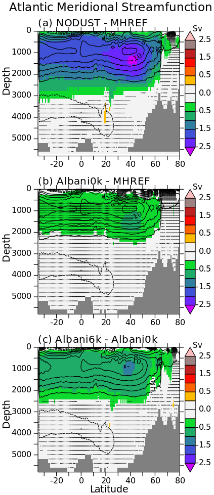
Figure 14 Differences in the meridional Atlantic overturning circulation (Sv) as a function of latitude (^∘) and depth (m) showing the effect of (a) NODUST, (b) Albani0k dust and (c) Albani6k dust on the mid-Holocene simulations. For (a) and (b) the reference is the reference mid-Holocene simulation MHREF, whereas for (c) the reference is the Albani0K mid-Holocene simulation. Stippling indicates values that are smaller than the centennial variability mid-Holocene estimate from MHREF. The test is done at each grid point, which is also a way to show the ocean model resolution with refined grid at the Equator and higher resolution at the ocean surface.

6 Discussion and conclusion

We analysed the impact of dust reduction on the mid-Holocene climate considering both an extreme case where dust is suppressed and a mid-Holocene dust reduction from interactive dust–climate simulations following the PMIP4 dust protocol (Otto-Bliesner et al., 2017). We use as a reference the new mid-Holocene simulations with the IPSLCM6-LR version of the IPSL model (Boucher et al., 2020), in which the spatial distribution of PI dust is prescribed from the IPSLCM6-LR CMIP6 PI simulations (Lurton et al., 2020). The comparison of this simulation, after the adjustment phase, with the previous simulations using the IPSLCM6A-LR version of the model (Dufresne et al., 2013; Kageyama et al., 2013a, b) highlights a few key regional differences arising from new developments in all the climate components and the higher resolution. Despite significant regional changes compared to previous mid-Holocene simulations or between the mid-Holocene dust experiments, the differences are not large enough to significantly improve the model results compared to Bartlein et al. (2011) temperature and precipitation reconstructions. Similar conclusions would also arise from comparisons with more recent reconstructions (see Brierley et al., 2020). The only noticeable improvement between the two IPSL model versions is in the representation of the coldest month temperature, which also tends to degrade the agreement for the annual mean (Fig. 6). Dust has different impacts in the different regions but does not affect the model–data differences much when model and data uncertainties are considered.

Nevertheless, we found systematic differences induced by dust between the sensitivity mid-Holocene dust experiments. Since we considered both a suppression of dust and the impact of dust reduction having different patterns compared to the original IPSL model dust distribution, we are able to test both the impact of dust reduction and the impact of dust pattern. The comparison with the standard mid-Holocene simulation reveals that the largest differences with the reference mid-Holocene simulation are induced by dust load pattern, which is characterised by an atmospheric dust reduction in Africa and an increase over the Middle East. These differences in dust pattern also have an impact on the climate response to mid-Holocene dust reduction. It thus stresses that the simulated dust pattern in the PI control simulation is also an important factor to consider when analysing the effect of dust in a different climate. It also implies that the effect of the mid-Holocene dust reduction cannot be simply deduced from the extreme no dust case, or by just considering dust reduction over a region.

These conclusions arise from detailed analyses of the dust radiative forcing and effect of dust on the Indian and African monsoons. The forcing differences induce both changes in local and global circulation resulting from the redistribution of MSE between source and sink regions. The fact that the Atlantic sector is most affected in all simulations compared to the other oceans reflects the dominant effect of dust over Africa and the fact that the dust pattern has a direct impact on induced atmospheric thermodynamics and dynamics changes. However, the magnitude and exact pattern over the tropical Atlantic depend on the teleconnection induced by the differences in dust load over the Middle East and Indian sector. It also stresses that differences in these forcing patterns, as well as the differences in dust representation and interaction with atmospheric radiation, need to be accounted for to be able to properly interpret the sensitivity of different climate models to dust forcing.

The response to our first two questions is thus that the dust induces a forcing that is about 10 times smaller than the insolation forcing but that it can be as large as the insolation forcing in very specific regions such as Africa where changes are the largest. The balance between the induced changes in West African and Indian monsoons depends on the dust pattern, which might explain inconsistent responses between models in their simulated relative changes between the monsoon rain intensity and location over India and Africa. A key difference between the two regions is also associated with orography and the fact that the warming/cooling over the southern flank of the Himalayas can induce different regional response over India than the one expected from radiative changes over the Tibetan plateau, whereas for Africa differences are led by dust properties and the linkages between atmospheric dust radiative effect and surface albedo.

Our results confirm previous results over Africa for the mid-Holocene period (Albani and Mahowald, 2019; Hopcroft and Valdes, 2019; Liu et al., 2018; Pausata et al., 2016; Thompson et al., 2019). At least part of the differences in the reported results are attributable to different dust optical properties and whether absorption by dust of longwave radiation was included. When the longwave effects are included, the presence of large particles in describing dust particle size distributions then becomes important. This is in line with studies using present day climate conditions that show how models using more absorbing optical properties tend to be associated with positive DRE at the top of the atmosphere (TOA) and increased Sahel precipitation, whereas models using less absorbing optical properties tend to produce the opposite effects (e.g. Albani et al., 2014; Balkanski et al., 2007; Lau et al., 2009; Miller et al., 2014; Strong et al., 2015). Recent observational constraints (e.g. Di Biagio et al., 2019; Kaufman et al., 2001; Sinyuk et al., 2003) indicate less absorbing dust optical properties than older estimates (e.g. the OPAC dataset from Hess et al., 1998) and the IPSL model dust radiative properties are consistent with satellite-based estimates (Patadia et al., 2009; Song et al., 2018).

Several studies also suggest that the increased monsoon induced by dust reduction during the mid-Holocene is effective only when the mid-Holocene increase in vegetation over the Sahel-Sahara region is considered (Pausata et al., 2016). This is not the case here, so other conclusions on the effect over Africa could be obtained with interactive vegetation with an increase instead of a decrease in monsoon extent and precipitation over Africa.

Another important point is the linkage with the Atlantic Ocean. It partly depends on the large-scale dust pattern, in particular from dust transport and feedbacks with the location of the ITCZ, and changes in precipitation in the West Atlantic. Our results show that depending on this region being affected or not in terms of winds and precipitation, there is a feedback on the Atlantic thermohaline circulation, which is slightly reduced in the simulations presented here. Similar connections with the thermohaline circulation have been discussed by other groups for the NODUST case (Zhang et al., 2021).This needs further investigation, because the dust pattern strongly affects the model response and because the signal is small and projects on the North Atlantic centennial variability. Very long simulations or ensembles would be needed to fully assess this effect.

Since the Atlantic sector is the one that is most affected by the impact of dust forcing whatever the pattern, palaeoclimate reconstructions over this sector seem particularly relevant to evaluate the results. This is why we selected the well-sampled regions in eastern North America and Western Europe in Fig. 6. However, a full assessment of the model realism can be only by done considering both the realism of the dust representation and forcing pattern in the reference climate (here pre-industrial) and the mid-Holocene changes. Therefore, future explorations need to consider the consistency of dust and land surface properties, and put more emphasis on dust outside Africa to properly assess pattern changes and the balance between the different atmospheric teleconnections and the way by which they induce changes in MSE large-scale gradients.

Appendix A: Simplified method to estimate dust forcing and feedback for shortwave radiation

The Taylor et al. (2007) method is only valid for the estimation of climate forcing for shortwave radiation. A first step consists of diagnosing how the surface albedo, atmospheric absorption and atmospheric scattering affect the planetary albedo for each climatic period.

For each simulation, the atmospheric absorption μ is estimated as

$$\begin{array}{}\text{(A1)}& \mathit{\mu }={\mathit{\alpha }}_{\mathrm{p}}+\left({\mathrm{SW}}_{\mathrm{si}}/{\mathrm{SW}}_{\mathrm{i}}\right)\left(\mathrm{1}-{\mathit{\alpha }}_{\mathrm{p}}\right)\end{array}$$

and the atmospheric scattering γ as

$$\begin{array}{}\text{(A2)}& \mathit{\gamma }={\displaystyle \frac{\mathit{\mu }-\left({\mathrm{SW}}_{\mathrm{si}}/{\mathrm{SW}}_{\mathrm{i}}\right)}{\mathit{\mu }-{\mathit{\alpha }}_{\mathrm{s}}\left({\mathrm{SW}}_{\mathrm{si}}/{\mathrm{SW}}_{\mathrm{i}}\right)}},\end{array}$$

where α_p and α_s represent respectively the planetary and the surface albedos, and SW_i and SW_si the incoming solar radiation at the top of the atmosphere (insolation) and at the surface. The planetary and surface albedos are computed from the downward and upward SW radiations.

The partial derivative to obtain the effect of the change in absorption between simulation 1 and simulation 2 is thus estimated as

$$\begin{array}{}\text{(A3)}& {\mathit{\alpha }}_{\mathrm{p}}\left({\mathit{\mu }}_{\mathrm{2}},\mathit{\gamma },{\mathit{\alpha }}_{\mathrm{s}}\right)-{\mathit{\alpha }}_{\mathrm{p}}\left({\mathit{\mu }}_{\mathrm{1}},\mathit{\gamma },{\mathit{\alpha }}_{\mathrm{s}}\right).\end{array}$$

The estimate of the changes in atmospheric scattering and in surface albedo are estimated following the same methodology. Figure A1 provides a comparison between this method and the online IRF estimates following the IRFMIP protocol. For the Taylor et al. (2007) method, the estimates are done using monthly outputs of the fully coupled simulations, whereas for the IRF atmosphere alone, simulations have been used (see Sect. 4). This comparison indicated that in this SW case the Taylor et al. (2007) approximation provides the same results as the more rigorous estimates.

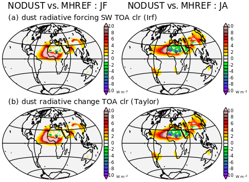
Figure A1 Comparisons of the shortwave radiative forcing estimated at the top of the atmosphere for clear sky conditions (SW TOA clr) using (a) the RFMIP protocol to compute instantaneous radiative forcing (IRF) or (b) the simplified Taylor et al. (2007) method from monthly model outputs. This figure only shows the results for NODUST compared to MHREF but the same agreements between the two methods is also found for the other simulations.