Terrestrial methane emissions from the Last Glacial Maximum to the preindustrial period

We investigate the changes in terrestrial natural methane emissions between the Last Glacial Maximum (LGM) and preindustrial (PI) periods by performing time-slice experiments with a methane-enabled version of MPI-ESM, the Max Planck Institute Earth System Model. We consider all natural sources of methane except for emissions from wild animals and geological sources, i.e. emissions from wetlands, fires, and termites. Changes are dominated by changes in tropical wetland emissions, with mid-to-high-latitude wetlands playing a secondary role, and all other natural sources being of minor importance. The emissions are determined by the interplay of vegetation productivity, a function of CO₂ and temperature; source area size, affected by sea level and ice sheet extent; and the state of the West African monsoon, with increased emissions from northern Africa during strong monsoon phases.

We show that it is possible to explain the difference in atmospheric methane between LGM and PI purely by changes in emissions. As emissions more than double between LGM and PI, changes in the atmospheric lifetime of CH₄, as proposed in other studies, are not required.

1 Introduction

The atmospheric concentration of methane underwent major changes in the time between the last glacial maximum (LGM) and preindustrial (PI) periods. Between LGM and 10 ka (before 1950 CE) atmospheric CH₄, as reconstructed from ice cores, nearly doubled from ∼ 380 ppb at LGM to 695 ppb at 10 ka (Köhler et al., 2017), with very rapid concentration changes of about 150 ppb occurring during the transitions from the Older Dryas to the Bølling–Allerød (BA), from the BA to the Younger Dryas (YD), and from the YD to the Preboreal (PB) or early Holocene (Fig. 1). Furthermore, while Holocene atmospheric CH₄ was very similar for 10 ka and PI (694 ppb, mean concentration for 300 to 200 a BP), CH₄ decreased linearly by 15 % from 10 to 5 ka and increased again linearly towards PI. If we assume that the atmospheric lifetime of CH₄ did not change dramatically between the LGM and the present, these changes in atmospheric CH₄ would require large changes in CH₄ emissions.

The change in methane between LGM and PI has been investigated in a number of studies. Some have used box models to explain the methane changes observed in ice cores. Recently Bock et al. (2017), for example, pointed to tropical wetlands as the main driver of glacial–interglacial CH₄ change from a study of methane isotopes from ice cores. In addition there are studies with comprehensive models. Kaplan (2002) investigated wetland CH₄ emissions during the LGM and the present using the BIOME4 model. He finds wetland emissions of 140 Tg CH₄ yr⁻¹ (1 Tg=10¹² g) for the present-day situation and 107 Tg CH₄ yr⁻¹ (−24 %) for the LGM, with wetland areas at the LGM slightly larger than at present. Valdes et al. (2005) performed time-slice experiments with the Hadley Centre Coupled Model (HadCM3), using the Sheffield Dynamic Global Vegetation Model (SDGVM) as a fire and wetland methane emission model, as well as an atmospheric chemistry model. They find PI wetland CH₄ emissions of 148 Tg CH₄ yr⁻¹ and LGM emissions of 108 Tg CH₄ yr⁻¹ (−27 %), with tropical sources changing rather little and Northern Hemisphere (NH) high latitudes contributing most of the change in emissions. Emissions from biomass burning changed from 11 Tg CH₄ yr⁻¹ at PI to 7 Tg CH₄ yr⁻¹ at LGM (−36 %), contributing to the total emission change from 199 Tg CH₄ yr⁻¹ at PI to 152 Tg CH₄ yr⁻¹ at LGM (−24 %). Weber et al. (2010) investigated wetland emissions for PI and LGM time slices with climate forcings from the Palaeoclimate Modelling Intercomparison Project (PMIP2) ensemble, which is applied to an offline wetland CH₄ model. They found an overall reduction by 29 %–42 %, with sources in the NH extratropics reduced by 51 %–60 %, while tropical sources were reduced by 22 %–36 %. Finally Hopcroft et al. (2017) investigated methane emission changes between LGM and PI using the Hadley Centre Global Environmental Model (HadGEM2-ES), considering wetlands, termites, and biomass burning as CH₄ sources, along with ocean and geological emissions. They obtain an overall source reduction by 28 %–42 %, with LGM wetland emissions (97 and 80 Tg CH₄ yr⁻¹ if northern peatlands are considered explicitly) reduced by 30 % in comparison to PI (138 Tg CH₄ yr⁻¹), and termite emissions reduced by 40 %.

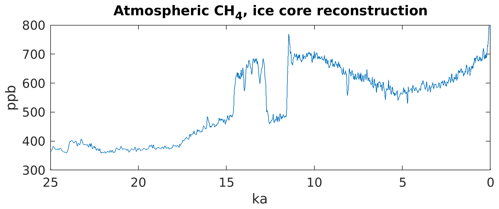
Figure 1 Atmospheric CH₄ as reconstructed from ice cores (Köhler et al., 2017, and references therein).

Studies of time slices between the LGM and PI are much sparser. Kaplan et al. (2006), using BIOME4-TG as a terrestrial methane emission model also determining emissions of biogenic volatile organic compounds (BVOCs) and an atmospheric chemistry model, investigated time slices every 1000 years from LGM to the present. They found that changes in atmospheric CH₄ are largely due to a changed lifetime, mainly through BVOC emission changes. Interestingly, they find a larger wetland area for the LGM than for present day, with emissions roughly the same (∼110 Tg CH₄ yr⁻¹), and an emission maximum around 10 ka. Finally, Singarayer et al. (2011) investigated methane for 65 time slices between 130 ka and PI with HadCM3 and SDGVM as a methane emission model. They point to orbital changes driving the methane increase between 5 ka and PI, as insolation increases in the SH tropics.

What these studies have in common is that they require (in some cases substantial) changes in the atmospheric lifetime of methane to explain the changes in atmospheric CH₄ reconstructed from ice cores. However, Levine et al. (2011) found very small changes in CH₄ lifetime between LGM and PI using the TOMCAT (Toulouse Off-line Model of Chemistry And Transport) atmospheric chemistry model, which had also been found by Murray et al. (2014) and Hopcroft et al. (2017), who investigated CH₄ lifetime using different atmospheric chemistry models. This small change in CH₄ lifetime arises from the balance of several competing influences, such as changes in reactive compounds, changes in reaction rates due to temperature changes, and changes in atmospheric OH due to water vapour changes. As a result, substantial changes in emissions are required to explain the changes in atmospheric methane as seen in ice cores, and none of the previous studies have managed to obtain the required changes in methane emissions, while fulfilling the constraints of the present-day methane budget at the same time.

In the present-day top-down CH₄ budget (Saunois et al., 2016), 59 % of the emissions are from anthropogenic sources can therefore be ignored for pre-anthropogenic times. However, 41 % (231 Tg CH₄ yr⁻¹) of the emissions are from natural sources and are therefore relevant for the entire time since the LGM. In the top-down budget, 167 Tg CH₄ yr⁻¹ (72 % of the natural emissions) are emitted from natural wetlands, and 64 Tg CH₄ yr⁻¹ come from “other” sources. These are not differentiated further in the top-down budget, but the bottom-up budget (Saunois et al., 2016) lists freshwater bodies (lakes), geological sources, wild animals, wildfires, permafrost soils, and vegetation as further onshore (land) sources and geological and other as offshore (oceanic) sources.

We aim to assess the changes in the natural sources of methane from the LGM to the present in order to determine the factors driving the changes in atmospheric CH₄. We use a methane-enabled version of MPI-ESM, the Max Planck Institute Earth System Model, to investigate changes in natural methane emissions for six time slices from the LGM to the present. In this model we include submodels for methane fluxes from wetlands, termites, and wildfires, but the other natural methane fluxes listed above cannot easily be derived from the climate model state; therefore, they are neglected for now. As time slice experiments very likely are not helpful for looking into the BA–YD and YD–PB transitions, we neglect these at present, focusing instead on the longer timescale changes in methane.

2 Model and experiments

2.1 MPI-ESM 1.2

We use the Max Planck Institute Earth System Model (MPI-ESM) in version 1.2 (Mauritsen et al., 2019), the version to be used in CMIP6. All experiments are performed in resolution T31GR30 (Mikolajewicz et al., 2018). In comparison to the CMIP5 version (Giorgetta et al., 2013), a number of errors were corrected in the atmosphere and ocean models, and the land surface scheme JSBACH (Reick et al., 2013; Brovkin et al., 2013; Schneck et al., 2013) has been updated with a multilayer hydrology scheme (Hagemann and Stacke, 2015), the SPITFIRE fire model (Thonicke et al., 2010; Lasslop et al., 2014), and the improved soil carbon model YASSO (Tuomi et al., 2009; Goll et al., 2015).

2.2 Wetland methane emission model

The present-day area that wetland methane emissions originate from is highly uncertain. The generation of methane in the soil is dependent on plant composition, carbon content, and carbon quality, essentially ecosystem properties, as well as the degree of anoxia in the soil, which depends on soil structure and water content, essentially hydrological properties. As there is no better estimate of the methane-generating area available, we determine the surface inundation and assume that this is a useful approximation of the areas where methane is generated.

2.2.1 Dynamic inundation model

We use an approach based on the TOPMODEL hydrological framework (Beven and Kirkby, 1979) to determine inundation extent dynamically. TOPMODEL is a conceptual rainfall–runoff model, based on the compound topographic index (CTI), ${\mathit{\chi }}_i=\ln \left({\mathit{\alpha }}_i/\tan \left({\mathit{\beta }}_i\right)\right)$, with α_i being a dimensionless index for the area draining through point i and β_i being the local slope at that point. TOPMODEL determines the local water table z_i at point i in relation to the grid-cell-mean water table $\overline{z}$:

$$\begin{array}{}\text{(1)}& z_i=\overline{z}+{\displaystyle \frac{\mathrm{1}}{f}}\left({\mathit{\chi }}_i-\overline{\mathit{\chi }}\right),\end{array}$$

with χ_i being the local CTI index at point i, $\overline{\mathit{\chi }}$ being the grid-cell-mean CTI index, and f being a parameter describing the exponential decline of transmissivity with depth. From Eq. (1) we determine the grid-cell fraction with a local water table depth z_i≥0. Since inundated areas become unreasonably large in some locations, we limit the valid range of CTI values by introducing the constraint χ_i≥χ_min following Stocker et al. (2014), with χ_min being constant in space and time. We assume this to be the inundated and therefore methane-emitting area A_inun, unless soils are frozen. In these cases we determine the fraction of liquid water in the soil f_liq from the soil temperature T_soil

$$f_{\mathrm{liq}}=\left\{\begin{array}{ll}\mathrm{1}& \forall T_{\mathrm{soil}}>\mathrm{273.65}\mathrm{K}\\ \mathrm{0.1}& \forall T_{\mathrm{soil}}<\mathrm{272.75}\mathrm{K}\\ \left(T_{\mathrm{soil}}-\mathrm{273.65}\mathrm{K}\right){\mathrm{K}}^{-\mathrm{1}}& \text{otherwise}\end{array}\right.$$

(limiting f_liq to $\mathrm{0.1}\le f_{\mathrm{liq}}\le \mathrm{1}$ for numerical reasons), and we determine the inundated area as $A_{\mathrm{inun}}^{\prime }=A_{\mathrm{inun}}\times f_{\mathrm{liq}}$, reducing the inundated area under freezing conditions, as frozen soils emit less methane, similar to Gedney and Cox (2003).

To determine the grid-cell-mean water table position $\stackrel{\mathrm{‾}}{z}$, we determine the layer saturation, ${\mathrm{\Psi }}_k={\mathrm{\Theta }}_k/{\mathrm{\Theta }}_{\mathrm{fc}}$, for each soil layer k by dividing the volumetric moisture content Θ_k by the field capacity Θ_fc. Starting from the bottom of the soil column, $\stackrel{\mathrm{‾}}{z}$ is located in the first soil layer l with layer saturation Ψ_l less than the saturation threshold Ψ_thres. The final water table position then is

$$\begin{array}{}\text{(2)}& \stackrel{\mathrm{‾}}{z}=z_{b,l}-{\mathrm{\Psi }}_l\mathrm{\Delta }{z}_l,\end{array}$$

with z_b,l being the bottom of soil layer l, and Δz_l being the height of soil layer l.

Values for f, χ_min, and Ψ_thres were determined from sensitivity experiments. In the experiments described here, we use f=2.6, χ_min=8.5, and Ψ_thres=0.95. Furthermore, comparison with remote-sensing data (Prigent et al., 2012) showed that inundated area in grid cells with a mean CTI index, $\overline{\mathit{\chi }}\le \mathrm{5.5}$, is negligible. Inundation is therefore only determined for grid cells with $\overline{\mathit{\chi }}>\mathrm{5.5}$.

We use the CTI index product by Marthews et al. (2015) for the CTI index at a resolution of 15 arcsec in all present-day land areas, while we determine CTI index values for shelf areas that are below sea level at present, but above sea level under glacial conditions, from the ETOPO1 dataset (Amante and Eakins, 2009) using the TOPMODEL library for R (Buytaert, 2011). In order to reduce storage requirements, we approximate the distribution of CTI values within a model grid cell by fitting a gamma distribution, following Sivapalan et al. (1987).

2.2.2 Wetland methane production and transport

We use the methane transport model by Riley et al. (2011) to determine wetland methane emissions, with minor modifications to adapt the model to the vegetation and carbon cycle representation in JSBACH. The Riley et al. (2011) model determines CO₂ and CH₄ production in the soil; transport of CO₂, CH₄, and O₂ through the three pathways (diffusion, ebullition, and and plant aerenchyma), and the oxidation of methane during transport.

Adaptations are described in the following. In the grid-cell fraction determined to be inundated by the inundation model, soil organic matter (SOM) is decomposed under anaerobic conditions in the YASSO soil carbon model (Goll et al., 2015), assuming a reduction of decomposition by a factor of 0.35 (Wania et al., 2010) in comparison to the aerobic case. As YASSO is a zero-dimensional representation of soil C processes, we distribute the decomposition product to the soil layers according to the root distribution from Jackson et al. (1996). Partitioning of the anaerobic decomposition product into CO₂ and CH₄ is temperature dependent, as in the original Riley model, with a baseline fraction of CH₄ production fCH₄=0.35 and a Q₁₀ factor for fCH₄ of Q₁₀=1.8, with a reference temperature of 295 K.

For each grid cell, the methane model determines CH₄ production and transport for two grid-cell fractions: the aerobic (non-inundated) and the anaerobic (inundated) fraction of the grid cell. If the inundated fraction changes, the amounts of CO₂, CH₄, and O₂ are conserved, transferring gases from the shrinking fraction to the growing fraction (proportional to the area change). While vegetation in JSBACH is determined for vegetation tiles, allowing a fractional coverage of plant functional types, the relevant properties (root distribution, SOM decomposition) are aggregated to grid-cell level for the methane transport model for performance reasons. Previous sensitivity experiments showed that differences to a tile-resolving formulation are negligible.

2.3 Methane emissions from wildfires

To determine methane emissions from wildfires, we use the biomass burned, diagnosed from the SPITFIRE module (Thonicke et al., 2010; Lasslop et al., 2014), and information on vegetation composition from the dynamical vegetation model. We use the methane emission factors from Kaiser et al. (2012), mapped to the JSBACH plant functional types, to determine the fraction of burned biomass emitted as methane. Therefore, changes in fire-related methane emissions are completely determined by changes in fire carbon emissions. Fire occurrence in the SPITFIRE model is determined as a function of flammability (higher under dryer or warmer conditions) and ignition probability, with ignition probability a function of lightning frequency and population density. We are currently limited to a fixed lightning distribution reflecting modern conditions, and we are assuming a population density of zero for all time slices earlier than preindustrial. Therefore, the main factors affecting fire-related methane emissions are carbon content and moisture conditions.

For PI and PD, we use an estimate of population density to determine the ignition probability, with ignition probability increasing with population density. However, under very high population densities it is assumed that fire suppression increases, thus decreasing fire probability and thus fire methane emissions, for very high population densities.

2.4 Methane emissions from termites

Methane emissions from termites are determined following the approach developed by Kirschke et al. (2013) and elaborated by Saunois et al. (2016), adapted for the use in a dynamical vegetation model. They distinguish between termite emissions from tropical and nontropical areas, using different parameterisations for determining the termite biomass, M_termite, and different emission factors for the two areas. For tropical areas, in our case defined as areas covered by the plant functional types (PFTs) tropical broadleaf evergreen tree, tropical broadleaf deciduous tree, and C₄ grass, we determine M_termite from the annual gross primary production GPP using $M_{\mathrm{termite}}=\mathrm{1.21}\times \exp \left(\text{GPP}\times \mathrm{0.0008}\right)$ (Kirschke et al., 2013). From M_termite we determine methane emissions using an emission factor of 2.8 $\mathrm{\mu }\mathrm{g}{\mathrm{CH}}_{\mathrm{4}}\mathrm{g}{\mathrm{Termite}}^{-\mathrm{1}}{\mathrm{h}}^{-\mathrm{1}}$ (Saunois et al., 2016). We define the nontropical areas with termite emissions, i.e. the areas where the tropical PFTs do not occur, as the areas suitable for temperate broadleaf evergreen trees using bioclimatic limits from Sitch et al. (2003): temperature of the coldest month, $T_{\mathrm{c}}>\mathrm{3}{}^{\circ }\mathrm{C}$, and a growing-degree-day (GDD) sum on the basis of 5 ^∘C (${\text{GDD}}_{\mathrm{5}}>\mathrm{1200}{}^{\circ }\mathrm{C}$). In these areas we assume a constant termite biomass, $M_{\mathrm{termite}}=\mathrm{3}\mathrm{g}{\mathrm{m}}^{-\mathrm{2}}$, and an emission factor of 1.7 $\mathrm{\mu }\mathrm{g}{\mathrm{CH}}_{\mathrm{4}}\mathrm{g}{\mathrm{Termite}}^{-\mathrm{1}}{\mathrm{h}}^{-\mathrm{1}}$ (Saunois et al., 2016). If croplands occur in any particular grid cell (not relevant for experiments presented here), emissions from the cropland tile are reduced to 40 % of the non-cropland grid-cell-mean emissions (also following Saunois et al., 2016).

2.5 Model experiments

We performed model experiments for five time slices at 20, 15, 10, 5 ka, and PI (in this case defined as the year 1850 CE). In addition we performed one transient historical experiment for the years 1850–2010 CE, starting from the PI time slice, in order to obtain a present-day (PD) climate state for evaluation purposes. All model experiments use prescribed orbital forcing from Berger (1978) and greenhouse gas forcings from Köhler et al. (2017). Orbital parameters and greenhouse gas concentrations are supplied to the model as 10-year mean values and are updated every 10 model years. Atmospheric aerosols were constant at 1850 conditions (Kinne et al., 2013), with the exception of the historical experiment, and we considered no anthropogenic land use.

The time slice experiments were initialised from a – so far unpublished – transient model experiment from 26 ka to PI with prescribed ice sheet extent from the GLAC-1D ice sheet reconstruction (Tarasov et al., 2012; Briggs et al., 2014; Ivanovic et al., 2016). This model experiment was initiated at 26 ka and run transiently from then to PI, i.e. the year 1850 CE. Ice sheet extent, as well as bathymetry and topography (Meccia and Mikolajewicz, 2018), and river routing (Riddick et al., 2018) were continuously updated throughout the deglaciation.

As the original transient experiments did not contain the methane code required for the experiments described here, the time slice experiments were initialised from the transient experiment with a three-step procedure to minimise climate drift from the original experiment. In the first step, all model components were initialised from the transient experiment, with the exception of the inundation and the methane model, which were initialised from scratch. The model was integrated for 20 years from this initial state. This was repeated for a second time, but using the inundation and methane states reached at the end of the initial experiment. In a third step, the model was run for 40 years, using the inundation and methane state reached at the end of step two, while using the conditions of the transient model experiments for all other model components. In this way we ensured that the state of the physical model, as well as the biogeochemistry, would always be as close as possible to the model state in the fully transient experiment.

We assess present-day (PD) conditions by performing a historical experiment for 1850–2010, initialised from the PI state of the transient deglaciation experiment. In the PD experiment we change greenhouse gas (GHG) and atmospheric aerosol transiently, using the Stevens et al. (2017) aerosol parameterisation, but we do not consider anthropogenic land use.

In order to further assess the changes in methane emissions between PI and 20 ka, we have performed additional sensitivity experiments, starting from the PI state. In experiment PI-C-LGM we impose 20 ka land carbon stocks in all grid points that are common between 20 ka and PI, and in experiment PI-CO2-LGM we impose 20 ka atmospheric CO₂ on the land biogeochemistry but not on the atmospheric physics. These experiments allow us to assess the effects of soil carbon and CO₂ changes on CH₄ emissions while keeping climate unchanged. In experiments PI-noQ10 and 20k-noQ10, finally, we modified the CH₄ production parameters (fCH₄=0.28 and Q₁₀=1.0) in such a way that partitioning between CO₂ and CH₄ is no longer temperature dependent, while giving similar total emissions in the PI state, thus mimicking the behaviour of models that do not take this factor into account.

Climate in the preindustrial state is very similar to the preindustrial control experiment described in Mauritsen et al. (2019) and Mikolajewicz et al. (2018). However, the orography used in the present experiments is different from that in the published preindustrial control experiments. The latter experiments employ a mean orography, while the orography in the transient deglaciation experiment that we used as starting conditions for our time slice experiments is an envelope orography. In the envelope orography, the grid-cell elevation is increased in comparison to the mean orography in order to better represent the influence of topography on atmospheric circulation in the coarse model resolution we are using. Technically, this is achieved by adding the standard deviation of elevation to the mean.

For all experiments, we analyse a 30-year mean climatology, with the exception of the PD experiment where we analyse a 10-year mean climatology obtained from years 2000 to 2009. All plots of absolute emissions are shown on the land–sea mask appropriate for the time interval under consideration, while difference plots show the outline of the PI land–sea mask.

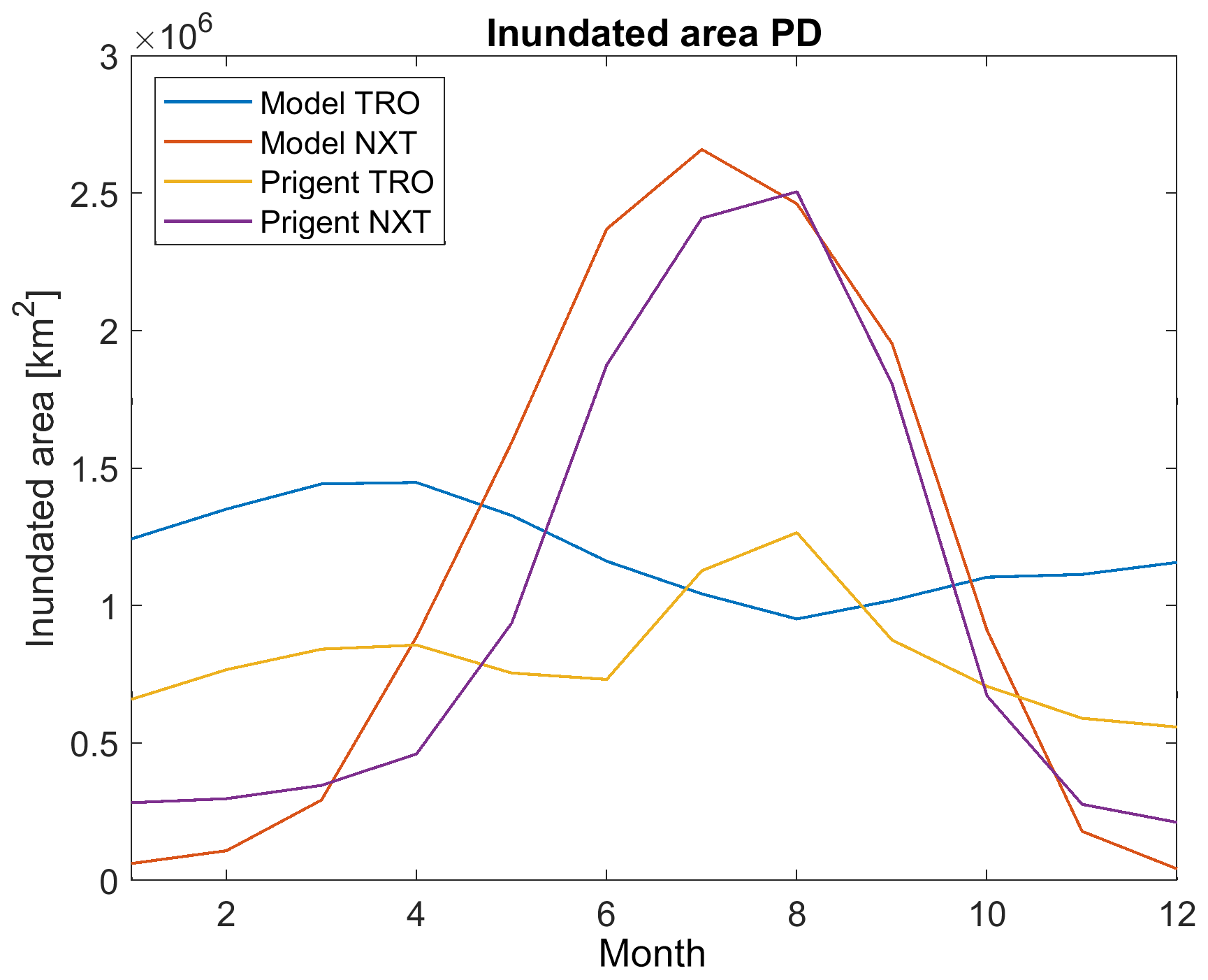
Figure 2 Climatology of monthly-mean inundated area for model years 2000–2009 and Prigent et al. (2012) observations (1993–2007), which is separated for the tropics (TRO) and NH extratropics (NXT).

3 Results and discussion

3.1 Evaluation of present-day methane emissions

3.1.1 Surface inundation

For the assessment of wetland methane emissions, the wetland area can to some extent be measured directly from satellites. Remote-sensing products of surface inundation are available, e.g. by Prigent et al. (2012) and Schroeder et al. (2015). To assess the quality of the modelled surface inundation, we rely on the Prigent et al. (2012) dataset. However, four points need to be considered when comparing these data to model results:

1. The remote-sensing process is unable to penetrate snow cover, so snow-covered areas are considered non-inundated.

2. The remote-sensing product shows all inundated areas, including areas flooded as a result of anthropogenic processes, such as the creation of reservoirs and rice paddies, which are not considered in the model.

3. Remote sensing may be unable to penetrate dense forest canopy, implying that inundation estimates may be biased in forested areas.

4. Not all methane-generating areas have water tables above the surface. Water tables in northern peatlands, for example, tend to be below the surface for part of the year, especially in the summer.

In order to make model output and remote-sensing data comparable, we therefore mask all snow-covered areas in the model output, and we use data on rice-growing areas by Monfreda et al. (2008) to mask all rice-growing areas from both the remote-sensing data and the model output. After these modifications, modelled inundated areas for the present-day period (mean over 2000–2009) are slightly larger than those observed by Prigent et al. (2012) (mean over 1993–2007) (Fig. 2). For the tropics (TRO, here for simplicity defined as latitudes between 30^∘ N and 30^∘ S) the annual mean inundated area is 1.2×10⁶ km² in the model results, while Prigent et al. (2012) show 0.8×10⁶ km². The seasonality is phase shifted, with the model showing the peak inundation in April, while Prigent et al. (2012) show the inundation peak in August (Fig. 2). For the glacier-free NH extratropics (NXT, here defined as north of 30^∘ N), the seasonality of inundation is similar in observations and model, but the summer peak in inundation is larger in the model (2.5×10⁶ km² for the JJA mean) than in the observations (2.3×10⁶ km²).

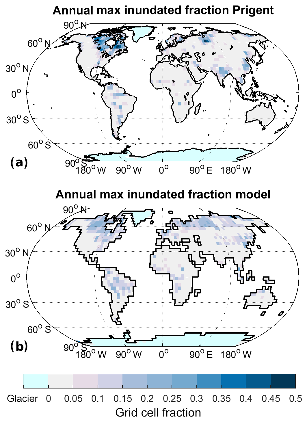
Figure 3 Annual maximum of mean monthly inundated fraction for Prigent et al. (2012) (a) and model (b).

Comparing the spatial pattern of the annual maximum inundation (Fig. 3), the overall pattern is rather similar, although two major differences are apparent: (1) the annual maximum inundation is more localised in the observations, while it is less clearly defined and reaching lower maximum values in the model, and (2) after removal of the rice-growing areas the model does not show a significant inundation maximum in India. These differences are likely due to the low resolution of the model we are employing. At higher resolutions, inundation becomes more localised and thus (1) appears clearly related to resolution and (2) is due to an underestimate of the Indian monsoon precipitation, also likely due to the low model resolution. We thus judge the methane-generating areas produced by the model as reasonable, keeping in mind the likely low bias of the remote-sensing inundation product.

As described above, we use the inundated area to determine the methane-emitting area. To evaluate the inundated areas leading to the wetland emissions, it has to be kept in mind that NXT emissions mainly are from the summer season, implying that the JJA (June, July, August) mean inundation is relevant for these, while the seasonality of TRO emissions is much less pronounced, implying that the annual mean inundation is relevant. In the following we therefore assess the effective inundated area, which is defined as the annual mean inundated area in tropical latitudes (TRO, between 30^∘ N and 30^∘ S), and the JJA (June, July, August) mean inundated area in the glacier-free NH extratropics (NXT, north of 30^∘ N). For the present-day climate state, the effective inundated area is 1.5×10⁶ km² in TRO and 2.6×10⁶ km² in NXT (differences to the numbers shown above due to the removal of rice-growing areas in the comparison to observations).

3.1.2 Natural methane emissions

So far it has not been possible to directly measure the quantity – surface methane fluxes – that we aim to assess in this publication on appropriate scales. Methane flux measurements exist for single sites on the scale of meters, mainly using measurement chambers, and for slightly larger scales, using eddy-covariance towers, but so far the scales relevant for global-scale modelling, from the model grid cell to global scales, have not been covered by direct methane flux measurements (Melton et al., 2013; Saunois et al., 2016; Poulter et al., 2017). For assessment of our model experiments, we therefore need to rely on global assessments (Saunois et al., 2016), and we can gain some additional insight from atmospheric inversions (Bousquet et al., 2011).

Under present-day (PD) climatic conditions (i.e. years 2000–2009 in the transient historical experiment), the model simulates wetland methane emissions of 222 Tg CH₄ yr⁻¹ (209–239 Tg CH₄ yr⁻¹), fire emissions of 17.6 Tg CH₄ yr⁻¹ (15.6–18.8 Tg CH₄ yr⁻¹), termite emissions of 11.7 Tg CH₄ yr⁻¹ (10.8–12.2 Tg CH₄ yr⁻¹), and a soil uptake of 17.5 Tg CH₄ yr⁻¹ (17.4–17.7 Tg CH₄ yr⁻¹). The values shown are mean values over the years 2000–2009 of the historical experiment, with the value in brackets giving the minimum and maximum annual emissions occurring in the model results. These values fall well within the ranges reported by Saunois et al. (2016), who report 153–227 Tg CH₄ yr⁻¹ for natural wetlands; 27–35 Tg CH₄ yr⁻¹ for biomass and biofuel burning, with biofuel burning making up 30 %–50 %; 3–15 Tg CH₄ yr⁻¹ for termites; and 9–47 Tg CH₄ yr⁻¹ for the soil uptake. Spatial patterns of modern emissions (Figs. B1 and B2) are generally similar to those shown by Saunois et al. (2016).

Furthermore, wetland methane emission estimates from atmospheric inversions (Bousquet et al., 2011) show that the majority (62 %–77 %) of the PD emissions come from the TRO region, while a much smaller part (20 %–33 %) are emitted from NXT. Of the modelled total wetland CH₄ emissions for PD conditions, 156 Tg CH₄ yr⁻¹ (70 %) is from TRO and 65 Tg CH₄ yr⁻¹ (29 %) is from NXT, while emissions from the SH extratropics (here defined as south of 30^∘ S) are negligible. The latitudinal distribution of modelled PD wetland methane emissions, therefore, is well within the range obtained from atmospheric inversions.

Overall, the PD state is rather similar to the PI state assessed in the following section, with very small differences in the distribution of emissions (Figs. B1 and B2), but generally higher methane emissions. At 287.4 K, the global mean temperature in the PD climate state is 0.5 K warmer than preindustrial (Table 1). Precipitation is similar, leading to negligible differences in the effective inundation. With 1140 Pg C, 8 % larger than PI, the global soil C stock is also rather similar. However, vegetation productivity is enhanced in comparison to PI, due to warmer temperatures and higher CO₂ concentrations. The net methane emissions in the PD climate are 29 % larger than PI (Table 2). Wetland methane emissions are 33 % larger, with a larger increase (+42 %) in TRO than in NXT (+16 %). Fire emissions are 18 % larger than PI, termite emissions increase by 66 %, and the soil uptake increases by 140 %. The latter increase is largely due to the higher atmospheric concentration of CH₄, which drives additional methane into the soils in comparison to the lower-CH₄ PI state. The larger fire emissions are mainly due to higher population densities in the 2000s than in 1850, although the very high population densities in eastern North America, Europe, and southern Asia are assumed to drive an increase in fire suppression in the SPITFIRE model (Lasslop et al., 2014). Thus fire emissions are decreased here, despite the general increase in most other places. Termite emissions are higher in the modern climate due to an increase in GPP under higher CO₂, while wetland emissions largely increase due to the higher temperatures of the modern climate, with CO₂-fertilisation playing an additional role.

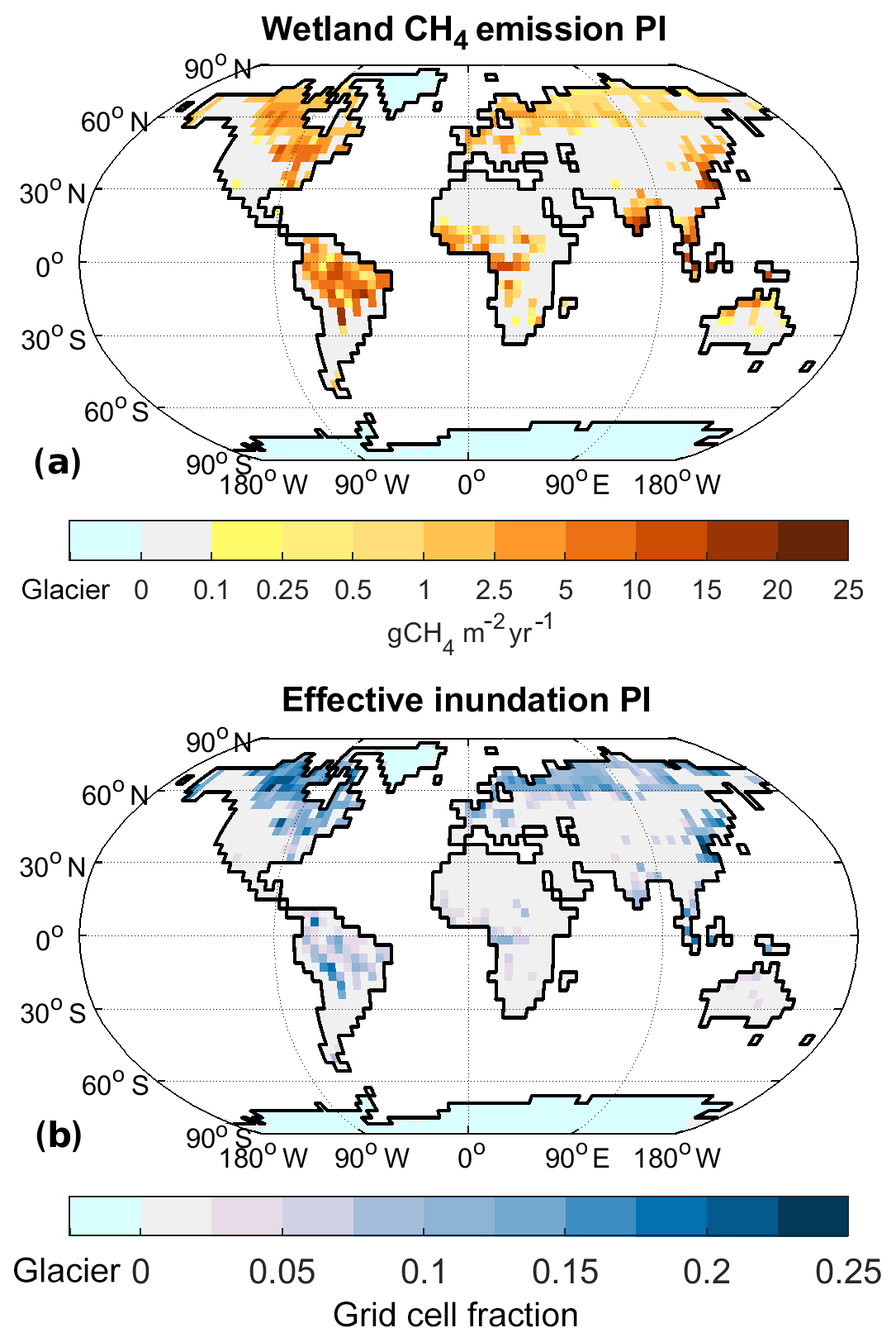
Figure 4 Wetland CH₄ emissions for preindustrial (PI) climate: annual emissions of CH₄ from wetlands (a) and effective inundation (b).

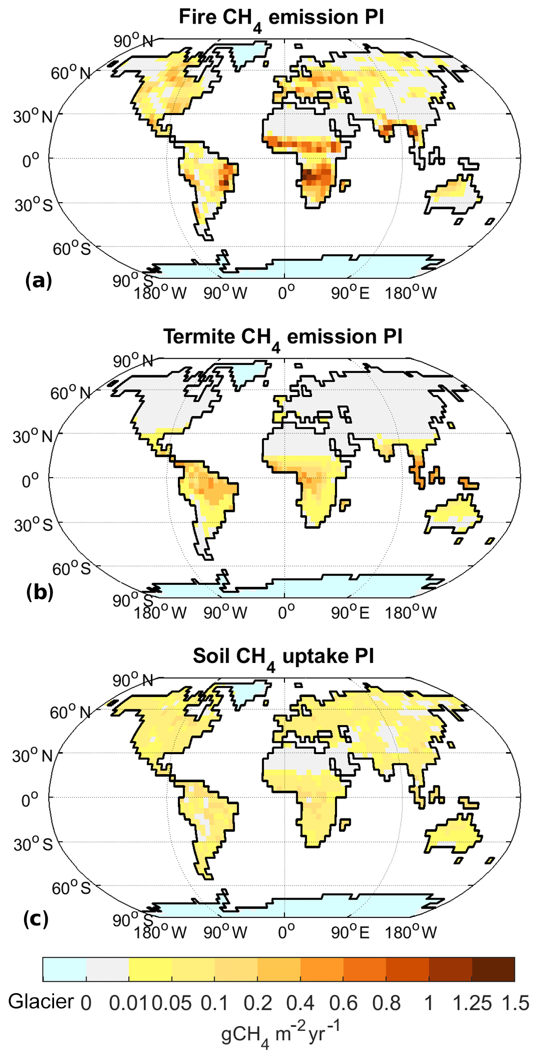
Figure 5 Non-wetland CH₄ emissions for PI climate: annual emissions of CH₄ from fires (a) and termites (b), as well as annual soil uptake of CH₄ (c). In comparison to other fluxes, soil uptake has the opposite direction (sign).

3.2 Preindustrial methane emissions

The climate in our PI experiment is very similar to the one described by Mikolajewicz et al. (2018). The global mean near-surface air temperature is 286.9 K (Table 1). The annual mean temperature in the TRO area, T_TRO, is 294.5 K, while T_NXT, the annual mean temperature in the NXT area, is 275.2 K. The NH ice sheet area is limited to Greenland, with the ice sheet having an area of 1.8×10⁶ km² in our model setup. Under these climatic boundary conditions, we obtain total net methane emissions of 181 Tg CH₄ yr⁻¹ (Table 2), with wetlands contributing 167 Tg CH₄ yr⁻¹ (Fig. 4a), fire and termites 15 and 7.0 Tg CH₄ yr⁻¹, respectively (Fig. 5a and b), and the soil uptake is 7.3 Tg CH₄ yr⁻¹ (Fig. 5c).

Wetland emissions, the dominant natural component of the terrestrial methane fluxes, mainly originate in TRO (110 Tg CH₄ yr⁻¹), while emissions from NXT are 56 Tg CH₄ yr⁻¹ (Table 2). The main factors determining wetland methane fluxes, apart from temperature, are the emitting area and the soil carbon stock that the soil respiration (and thus methane production) is derived from. In the PI state the global effective inundated area is 4.0×10⁶ km² (Fig. 4b), of which 2.7×10⁶ km² is located in NXT, while 1.3×10⁶ km² is in TRO (Table 1). For soil carbon, on the other hand, the global stock is 1054 Pg C (1 Pg=10¹⁵ g), with most of the soil carbon (588 Pg C) located in NXT, while it is 439 Pg C in TRO.

Methane emissions from fires (Fig. 5a) closely follow the fire distribution, with most fire methane emissions coming from subtropical Africa and South America, although some emissions also originate in North America, Southern Europe, and southern Asia. Termite emissions, on the other hand, mainly originate from tropical regions, especially southern Asia, with minor contributions from subtropical regions on all continents (Fig. 5b). Methane uptake by upland soils (Fig. 5c), finally, is distributed widely with no large regional variations.

3.3 Wetland methane emissions

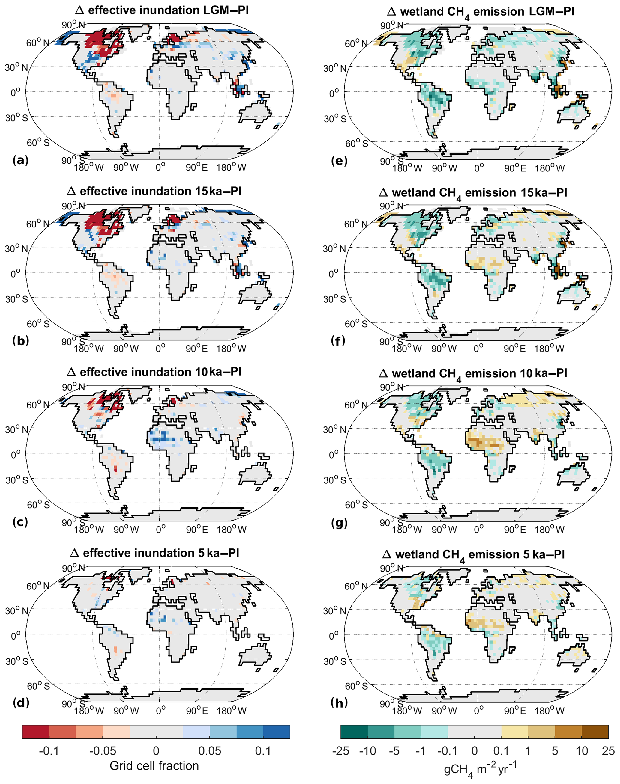
Figure 6 Change in effective inundation and wetland methane emissions for past climate states: (a–d) inundation difference to PI, (e–h) CH₄ emission difference to PI. (a, e) LGM, (b, f) 15 ka, (c, g) 10 ka, and (d, h) 5 ka.

Table 1 Climate and areas given in experiments. Global mean annual temperature T_GM, TRO temperature T_TRO, and NXT temperature T_NXT (all in kelvin). Global nonglaciated land area A_nonglac, TRO area A_TRO, NXT area A_NXT, TRO effective inundated area I_TRO, and NXT effective inundated area I_NXT (all in 10⁶ km²).

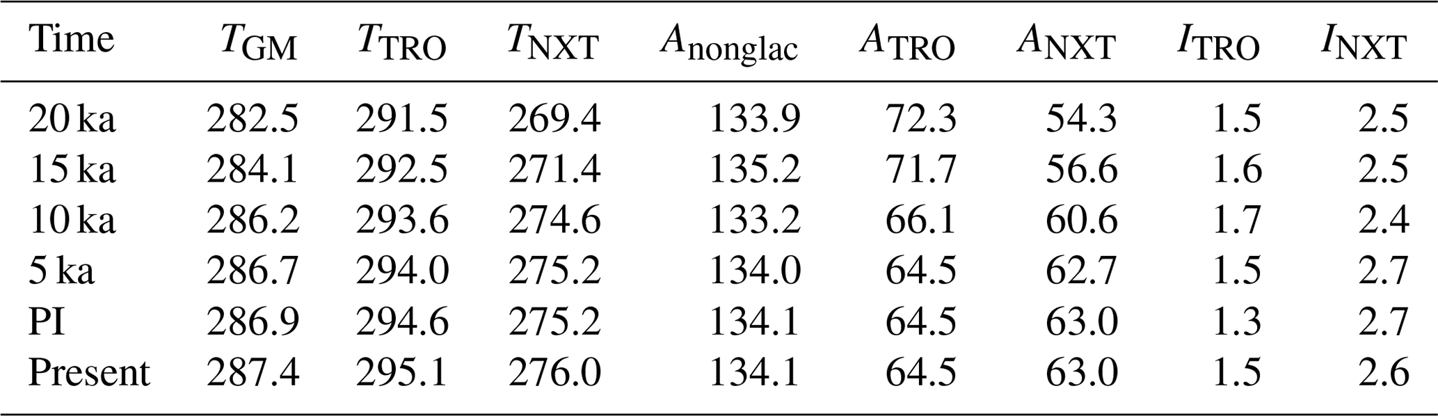
Under LGM boundary conditions the global mean temperature is 4.4 K colder than under PI conditions (Table 1). Extensive glaciers cover the NH extratropics and sea level is lower, leading to a 15 % increase in total land area, although total glacier-free area is nearly identical (Table 1). Thus, the TRO area, A_TRO, is 12 % larger than PI, while the NXT area, A_NXT (by definition glacier free), is 14 % smaller. The temperature decrease is less pronounced in TRO (−3.1 K) than in NXT (−5.8 K). Precipitation decreases by 10 % in the global mean, with an 11 % decrease in TRO and a 19 % decrease in NXT. TRO effective inundated area I_TRO thus increases by 19 % (Table 1, Figs. 6a, B3a), while NXT effective inundated area I_NXT decreases by 6 %. The global soil C stock is 617 Pg C, substantially smaller (−41 %) than at PI, with the decrease smaller in TRO (−33 %) than in NXT (−49 %). As a result of these climate changes, wetland methane emissions decrease by 51 % (Table 2, Figs. 6e, B3e), with a TRO emission decrease of 47 %, while NXT emissions decrease by 59 %, with the majority of the latter emissions coming from areas in East Asia adjacent to the Yellow Sea and North America south of the Laurentide ice sheet. The wetland CH₄ emissions therefore decrease nearly everywhere (Fig. 6e), with one major exception: the continental shelf areas that are exposed due to the lower sea level become significant sources of methane, especially in Indonesia but also in Africa and Asia. At 29 Tg CH₄ yr⁻¹, they contribute about 35 % of the total wetland CH₄ emissions at the LGM.

Analysing the factors leading to the reduction in 20 ka wetland CH₄ emissions further (see Appendix A for details), we can explain a reduction of emissions by 42 % in comparison to PI by the changes in land carbon and atmospheric CO₂. Changes in temperature lead to a further reduction by about 20 %, while changes in available land points actually lead to an increase in emissions, as the available land points in the northern high latitudes (with low emissions) are reduced, while the available land points in the tropics (with high emissions) are increased.

For 15 ka, the global mean temperature change is −2.8 K relative to PI. NH ice sheet extent is 24 % lower than at LGM but still extensive. The total land area is 12 % larger than PI due to the lower sea level, but A_nonglac is only larger by 1 %. A_NXT is thus reduced by 10 % (Table 1), while A_TRO is increased by 11 %. The change in T_TRO is −2.0 K (Table 1), while it is −3.8 K for T_NXT. Precipitation decreases by 6 % in the global mean, with a 4 % decrease in TRO and a 10 % decrease in NXT. Precipitation in NH Africa is slightly increased due to a stronger West African monsoon. I_TRO thus is larger by 29 %, while I_NXT is 8 % smaller than PI (Table 1, Figs. 6b, B3b). Global soil C is at 815 Pg C (−23 %), with TRO C stocks at 398 Pg C (−9 %), while NXT stocks are at 392 Pg C (−33 %). Total wetland methane emissions decrease by −22 % as a result, with TRO emissions decreasing by 17 % and NXT emissions of by 33 % (Table 2, Figs. 6f, B3f). In contrast to the LGM situation, there is an increase in CH₄ emissions from NH (sub)tropical Africa (Fig. 6f) to 19 Tg CH₄ yr⁻¹ (+58 %), due to wetter conditions in the Sahel area. The exposed shelf areas emit about 38 Tg CH₄ yr⁻¹ overall (29 % of the total emissions).

For 10 ka, our model indicates a global mean temperature change of −0.7 K (Table 1). Glacial area is much reduced in comparison to the LGM, but remains of the Laurentide ice sheet still cover parts of northeastern Canada, leading to a lower sea level than at PI. Thus, the total land area is 3 % larger than at PI (A_nonglac−1 %), with A_TRO 3 % larger due to lower sea level and A_NXT 4 % smaller due to the remaining ice sheet coverage. The temperature decrease is larger in TRO (−1.0 K) than in NXT (−0.6 K). Precipitation is near PI levels in the global mean (−1 %), with a 6 % increase in TRO and a 1 % decrease in NXT. Precipitation in NH Africa is strongly increased due to a strong West African monsoon. I_TRO is increased by 35 %, mainly due to the wetter conditions in north Africa, while I_NXT is decreased by 12 % in NXT (Table 1, Figs. 6c, B3c). Global soil C is at 983 Pg C, quite near the PI total stock (−7 %), with a TRO soil C stock of 449 Pg C (+2 %) and a NXT stock of 510 Pg C (−13 %). As a result, wetland CH₄ emissions are very similar to PI (Table 2), with +7 % in TRO wetland emissions and −14 % in NXT emissions (Table 2, Figs. 6g, B3g). The increase in TRO emissions mainly occurs in the Sahel area, where the West African monsoon is strongly increased, leading to more precipitation, increased inundated area, and more biomass and soil C. Emissions from NH Africa are 37 Tg CH₄ yr⁻¹ (+208 %), which is an increase larger than the total increase in TRO emissions. Emissions from the (small) exposed shelf areas are at 8 Tg CH₄ yr⁻¹ (5 % of the total wetland CH₄ emissions). NXT emissions are smaller than PI in North America and Europe, but they are larger than PI in northern Asia, due to the summer warming from the changed insolation at 10 ka.

At 5 ka, global mean temperature change is at −0.2 K (Table 1). Ice sheet areas are as in the PI state; thus, TRO and NXT areas are unchanged. T_TRO is slightly lower (−0.6 K), but T_NXT is very similar to PI. Precipitation changes are very small in the global mean, with a 4 % increase in TRO and a 2 % increase in NXT, with the West African monsoon slightly stronger than PI. I_TRO increases by 15 %, while I_NXT decreases by 1 % (Table 1, Figs. 6d, B3d). Global soil C stocks are 1043 Pg C, slightly smaller than preindustrial (−1 %), with an increase by 4 % in TRO, especially in the southern Sahel region, while NXT is 4 % lower than PI. Total wetland methane emissions increase by 2 %, with TRO and NXT wetland emissions both increasing by 2 % (Table 2). Emissions from NH Africa are 21 Tg CH₄ yr⁻¹ (+75 % compared to PI, 19 % of TRO emissions), while emissions from the SH are generally decreased. NXT emissions are decreased in northern North America, while emissions from northern Asia and southern North America are increased.

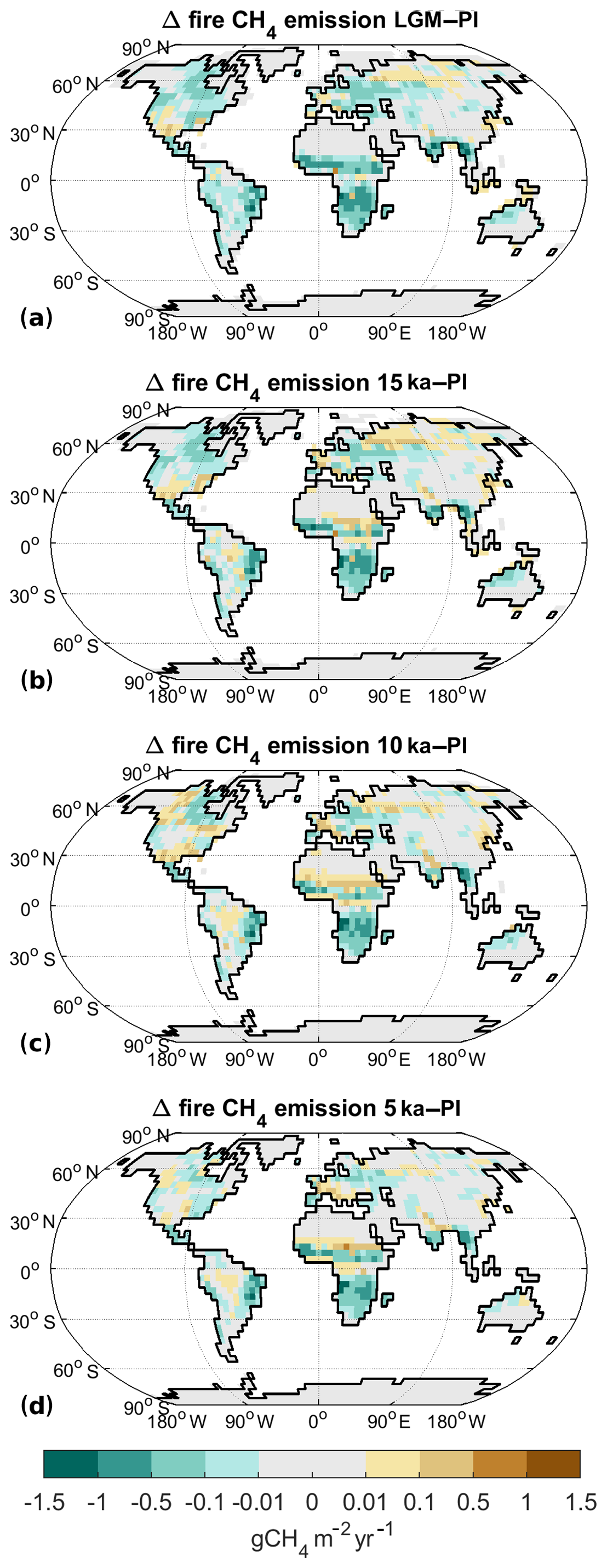
Figure 7 Difference in wildfire methane emissions to preindustrial for (a) LGM, (b) 15 ka, (c) 10 ka, and (d) 5 ka.

3.4 Methane emissions from wildfires

For all time slices before PI, we assume that no humans were present, leading to a generally decreased probability of fire ignition in comparison to PI and PD. For the LGM (Fig. 7a), fire CH₄ emissions (Table 2) are 73 % smaller. As biomass is reduced strongly under the cold and low-CO₂ conditions of the LGM, fire-related C emissions are also reduced. At 15 ka (Fig. 7b) fire emissions are 53 % lower than PI, while they are 40 % lower at 10 ka (Fig. 7c). Generally, the spatial pattern of emission changes at 15 and 10 ka mainly reflects precipitation changes: enhanced emissions occur in areas where precipitation is reduced, enhancing vegetation flammability. In the Sahel area, this relationship is different, though. Here, the enhanced rainfall leads to an increase in vegetation cover, especially grass cover. As a result, more biomass is available for combustion, leading to enhanced emissions. At 5 ka, finally, fire emissions are reduced by 45 %. As climate is already relatively similar to the PI situation, the main reason for the fire emission reduction here is the smaller ignition probability due to the absence of humans.

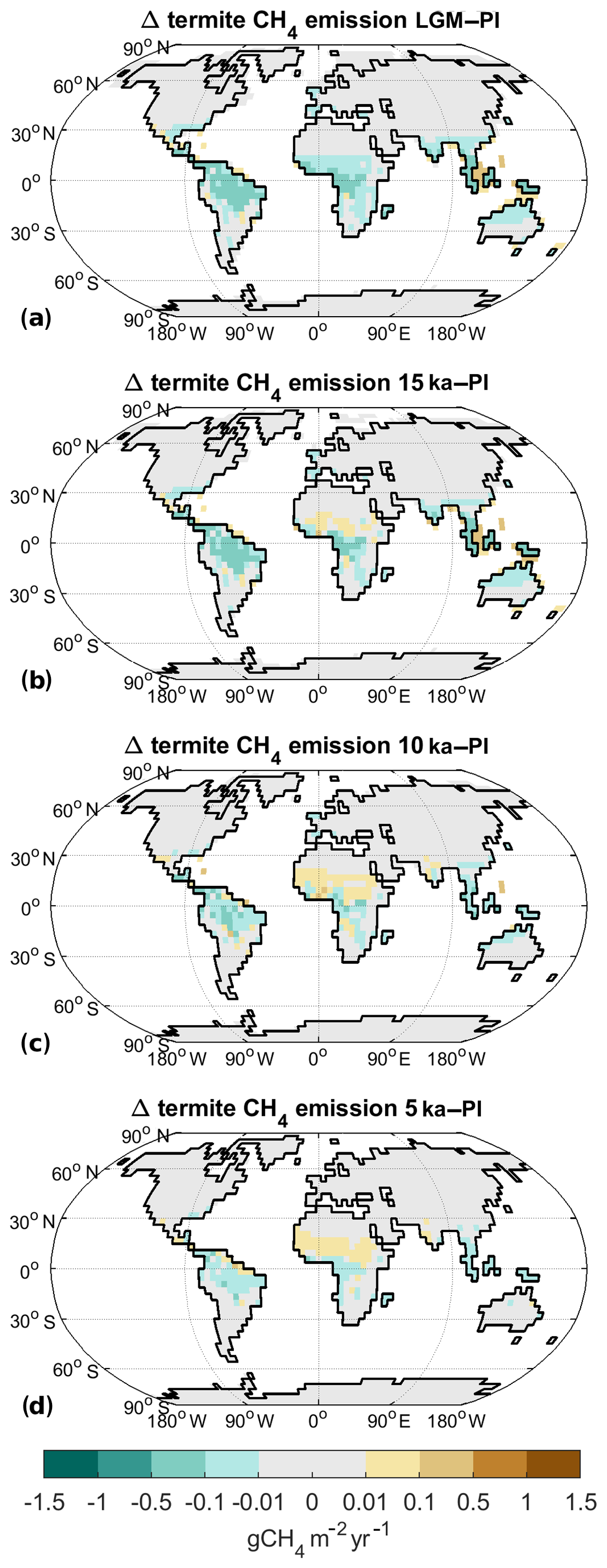
Figure 8 Difference in termite methane emissions to preindustrial for (a) LGM, (b) 15 ka, (c) 10 ka, and (d) 5 ka.

3.5 Methane emissions from termites

Termite emissions are mainly determined by gross primary productivity (GPP) in tropical and subtropical areas. The lower atmospheric CO₂ and temperature under LGM conditions decrease GPP everywhere. Therefore, termite CH₄ emissions are reduced by 58 % relative to the PI level (Table 2). For 15 ka, there also is a general reduction in termite emissions, with 4.6 Tg CH₄ yr⁻¹ in total (−34 %). However, the enhanced rainfall in the Sahel area leads to an increase in termite methane in this area. The latter is similar at 10 ka, where total emissions are 13 % smaller in comparison to PI. The enhanced productivity in the Sahel, therefore, more than compensates the decrease in termite methane from the Amazon and African rain forests. At 5 ka, finally, termite emissions are slightly smaller than PI (−7 %), with minor decreases in the rain forest areas and a slight increase in the Sahel.

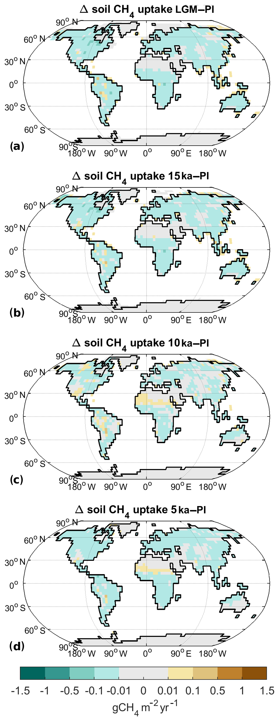
Figure 9 Difference in methane soil uptake to preindustrial for (a) LGM, (b) 15 ka, (c) 10 ka, and (d) 5 ka.

3.6 Methane uptake by soils

The soil continually exchanges methane and oxygen with the atmosphere through diffusion. In areas where soil conditions are aerobic, methane concentrations in the soil are smaller than atmospheric concentrations, thus driving a flux of methane into the soil. In the soil the methane is oxidised, with oxidation rates dependent on the concentrations of CH₄ and O₂, as well as temperature. The gas exchange between soil and atmosphere is also modified by the presence of plants, as some plant tissues can transport gases between plant roots and leaves.

In our experiments, we find that the soil uptake of methane is to a large extent determined by the gradient of methane between soil and atmosphere. Thus higher atmospheric concentrations of methane directly lead to a larger soil uptake of methane. Under LGM conditions, the atmospheric CH₄ concentration is 370 ppb, which is slightly less than half the PI concentration. Consequently soil methane uptake decreases by 68 % compared to PI (Table 2), with decreased temperatures being an additional factor (Fig. 9a). At 15 ka (atmospheric CH₄ of 464 ppb), the soil uptake is 52 % smaller, while it is changed by −14 % at 10 ka (688 ppb) and −28 % at 5 ka (579 ppb). Spatially, the change in methane uptake is rather uniform, showing a similar reduction in uptake in most locations (Fig. 9). The exception to this is, once again, the Sahel area, which shows an increase in methane uptake most pronounced for 10 ka (Fig. 9c) but also for 5 ka (Fig. 9d). For these time slices, the increase in vegetation cover in the Sahel region leads to a localised increase in methane uptake.

Figure 10 Components of the net CH₄ emissions for all time slices. Soil uptake of CH₄ is shown as a negative flux. Calculation of implied emissions and error bar as detailed in the text.

3.7 Time slice comparison

The net natural methane flux, i.e. the sum of all flux components, increases from 86 Tg CH₄ yr⁻¹ at 20 ka (−52 % compared to PI) to 181 Tg CH₄ yr⁻¹ in the PI state (and 233 Tg CH₄ yr⁻¹ (+29 %) at present).

Table 2 Methane emissions for all time slices (in Tg CH₄ yr⁻¹). Shown are soil uptake, total wetland emissions, fire and termite emissions, net emissions, and wetland emissions from TRO and NXT.

The wetland emissions from TRO are the most important component of the net methane flux during all time slices. Their contribution is smallest at PI (61 % of total net emissions) and largest at 20 ka (67 %). The contribution from NXT ranges from 27 % at 20 ka to 32 % at 5 ka. Fire emissions make up 4 %–5 % in the purely natural states between 20 and 5 ka and about 8 % for the anthropogenically influenced states at PI and PD. Termite emissions make up between 3.4 % and 5.0 % of net emissions, and soil uptake reduces the emissions by between 2.5 % at 15 ka and 7.0 % in the PD state (Table 2). Our modelled CH₄ emissions are also supported by the interpolar gradient in methane, as reconstructed by Baumgartner et al. (2012) for the LGM and Mitchell et al. (2013) for PI. Mitchell et al. infer tropical emissions of about 125 Tg CH₄ yr⁻¹ and NXT emissions of about 66 Tg CH₄ yr⁻¹ for the PI state (estimated from their Fig. 1), while Baumgartner et al. infer tropical emissions of about 60 Tg CH₄ yr⁻¹ and NXT emissions of about 25 Tg CH₄ yr⁻¹ for the LGM (estimated from their Fig. 5b).

In the modelled emissions, we are missing two components of the natural methane cycle: wild animals and geological sources. For geological emissions, estimates vary widely, with bottom-up estimates in Saunois et al. (2016) of 35–76 Tg CH₄ yr⁻¹ for on- and offshore sources, while Petrenko et al. (2017), estimating methane ¹⁴C for the YD from ice cores, constrain methane stemming from old carbon reservoirs to the range 0–18.1 Tg CH₄ yr⁻¹ at the YD. These fluxes likely are constant in time, although there might be changes during periods of sea level rise and fall, as hypothesised for CO₂ by Huybers and Langmuir (2009). Methane emissions from wild animals, especially ruminants, are very difficult to estimate; current estimates for the present span a range 2–15 Tg CH₄ yr⁻¹ (Saunois et al., 2016), and estimates for other time slices are even less confident but might be of the order of 15–20 Tg CH₄ yr⁻¹ for times before significant human influence (Chappellaz et al., 1993). In principle, these emissions should somehow be related to the net primary productivity, as this would determine the carrying capacity of the ecosystem, implying smaller fluxes in the glacial than in the Holocene. Adopting the ice-core-based estimate by Petrenko et al. (2017) for the geological fluxes, we can thus hypothesise these to be $\mathrm{9}\pm \mathrm{9}\mathrm{Tg}{\mathrm{CH}}_{\mathrm{4}}{\mathrm{yr}}^{-\mathrm{1}}$, while wild animals might add $\mathrm{15}\pm \mathrm{10}\mathrm{Tg}{\mathrm{CH}}_{\mathrm{4}}{\mathrm{yr}}^{-\mathrm{1}}$. The total unaccounted fluxes might therefore be of the order of $\mathrm{24}\pm \mathrm{19}\mathrm{Tg}{\mathrm{CH}}_{\mathrm{4}}{\mathrm{yr}}^{-\mathrm{1}}$.

To compare the net fluxes to the reconstructed atmospheric CH₄ concentrations from ice cores, we determined the implied methane emissions (Fig. 10). We converted the methane concentrations into a methane burden, using a conversion factor of 2.767 Tg CH₄ ppb⁻¹ (Dlugokencky et al., 1998). With a tropospheric lifetime of 9.3 years (range given 7.1–10.6 years) – an approximation for the present-day situation (Saunois et al., 2016) – we then determined the methane flux required to obtain the CH₄ concentration reconstructed for all time slices except the present-day period, which is dominated by anthropogenic emissions. From this flux, we subtracted the unaccounted sources, as described above, to determine the implied emissions. Uncertainties from the unaccounted fluxes are represented as error bars; however, the uncertainty in tropospheric lifetime is not considered here but would roughly add another 15 %.

Comparing the modelled net emissions to the implied emissions (Fig. 10), the modelled fluxes are within the range of uncertainty for all time slices except for 15 and 5 ka, with modelled net emissions larger than the implied fluxes for these time slices. The net emissions increase by more than 100 % going from 20 to 10 ka (and PI); we can thus explain the methane increase from LGM to Holocene with CH₄ emissions only and not requiring changes in methane lifetime. However, we so far cannot explain the Holocene changes in atmospheric CH₄: decreasing between 10 and 5 ka and increasing subsequently. For 5 ka, Singarayer et al. (2011) explain the decreased emissions in comparison to PI by reduced SH precipitation, leading to lower wetland CH₄ emissions. We obtain a similar result in our model, with SH wetland emissions reduced by 10 Tg CH₄ yr⁻¹ in comparison to PI. However, our NH emissions are substantially larger than at PI, due to substantial increases in Sahel precipitation and wetland emissions. We assume that this is due to an overestimate of the West African monsoon and its impact on African methane emissions, as a general reduction in the West African monsoon would lead to decreases in TRO emissions for 15, 10, and 5 ka, bringing model results more in line with the implied emissions determined from ice core CH₄. However, this is speculative at this point and would require further experiments.

4 Conclusions

In this assessment we considered all natural emissions of methane, with the exception of emissions from wild animals and geological sources. In our experiments we found that it is possible to explain the difference between LGM (20 ka) and PI methane concentrations purely by changes in the emissions of methane, without requiring changes in the atmospheric lifetime of CH₄. The time slice experiments we performed suggest that there are three main drivers to changes in methane emissions over the time from the LGM to the present:

1. The first main driver is global mean temperature and CO₂. Higher atmospheric CO₂ concentrations increase net primary production (NPP) and thus also soil carbon available for anaerobic decomposition to CH₄. Similarly, higher global mean temperature also increases NPP and soil C decomposition, and it furthermore increases the ratio of CH₄ to CO₂ production in anaerobic decomposition. Thus, higher atmospheric CO₂ and higher global mean temperature lead to larger wetland emissions of CH₄. This affects emissions from wildfires and termites in a similar way, as fire C release is dependent on biomass and termite biomass is dependent on GPP and thus CO₂ and temperature.

2. The second main driver is ice sheet area and sea level. Larger ice sheets remove CH₄ sources in the Northern Hemisphere extratropics as these are covered by the ice sheets, which is especially important for wetland methane emissions from North America. At the same time large ice sheets lower sea level, enlarging tropical wetland area as the continental shelf is exposed and becomes a significant source of methane. This is mainly relevant in the tropics, as high-latitude shelf areas exposed under glacial conditions, e.g. the Laptev Sea shelf, experience extremely cold conditions in glacial climate, leading to negligible methane emissions. Exposed shelf areas in Indonesia, Africa, and South America, on the other hand, emit significant amounts of methane. Thus lower sea level leads to larger emitting areas and thus higher emissions of methane.

3. The third main driver is the West African monsoon. During the time slices when the West African monsoon is stronger than at present, i.e. at 15, 10, and 5 ka, precipitation in the Sahel region is significantly enhanced in comparison to the PI state, leading to an increase in vegetation cover, productivity, and biomass burning. As a result, methane emissions at these times are stronger than at present, leading to a significant increase in (sub)tropical CH₄ emissions, with all natural methane sources increased.

For methane emissions from wildfires, a further factor influencing the emissions is the human population density, as this strongly affects the fire probability in the SPITFIRE model employed in JSBACH (Fig. 10). The soil uptake of methane, on the other hand, is strongly dependent on the atmospheric concentration of methane (Fig. 10).

The changes in methane from LGM to the present are dominated by changes in tropical wetland emissions, with mid- and high-latitude wetland emissions being a significant but secondary factor, gaining in importance as the high latitudes become ice free. Wetland emissions make up 93 %–96 % of the net CH₄ flux, and all other methane sources are thus of minor importance.

Appendix A: Sensitivity of LGM wetland fluxes

The large changes in wetland methane emissions between PI and 20 ka are due to a combination of several factors. While climate change is the ultimate cause of all of these influences, it is possible to identify several individual factors that likely contributed, and may have led to, the larger changes in methane emissions than in some previous studies. (1) Due to sea level fall and glacier expansion, the ice-free land domain changes appreciably; (2) reduced soil carbon at 20 ka leads to less organic matter being available to be decomposed; and (3) reduced atmospheric CO₂ leads to lower vegetation productivity and litterfall, and thus reducing both the plant transport of methane and the availability of soil organic matter for decomposition. In addition, (4) the temperature dependence of the ratio of CH₄ and CO₂ production in anaerobic soil organic matter decomposition is a relatively recent finding not considered in all methane transport models yet (Xu et al., 2016), and it may also have played a role. In order to further assess these factors, we conducted a set of sensitivity experiments, as detailed in Sect. 2.5.

The ice-free land domain changes appreciably between PI and 20 ka (Fig. A1), with expanded ice sheets reducing the available area in the NH high latitudes, and lower sea level exposing additional land both in the high latitudes and in the tropics. Restricting analysis to the glacier-free land points common to both the PI and 20 ka time slices leads to a reduction in emissions by 16 % for the PI state and by 35 % for the LGM state (Table A1). The change in ice sheets and sea level thus leads to an increase in 20 ka wetland emissions compared to a state where the land–sea mask does not change, as some of the additional 20 ka grid points are located in the tropics, where large amounts of methane are emitted.

Table A1 Sensitivity experiment results: wetland CH₄ emissions (Tg CH₄ yr⁻¹) on all grid points (AP), emission change ( %) with regard to PI state on all points, wetland emissions (Tg CH₄ yr⁻¹) on the common grid points (CP), emission change ( %) with regard to PI state on the common points, and emission change between common points and all points (%). The reference state for emission change in experiment 20k-noQ10 is the 20 ka state.

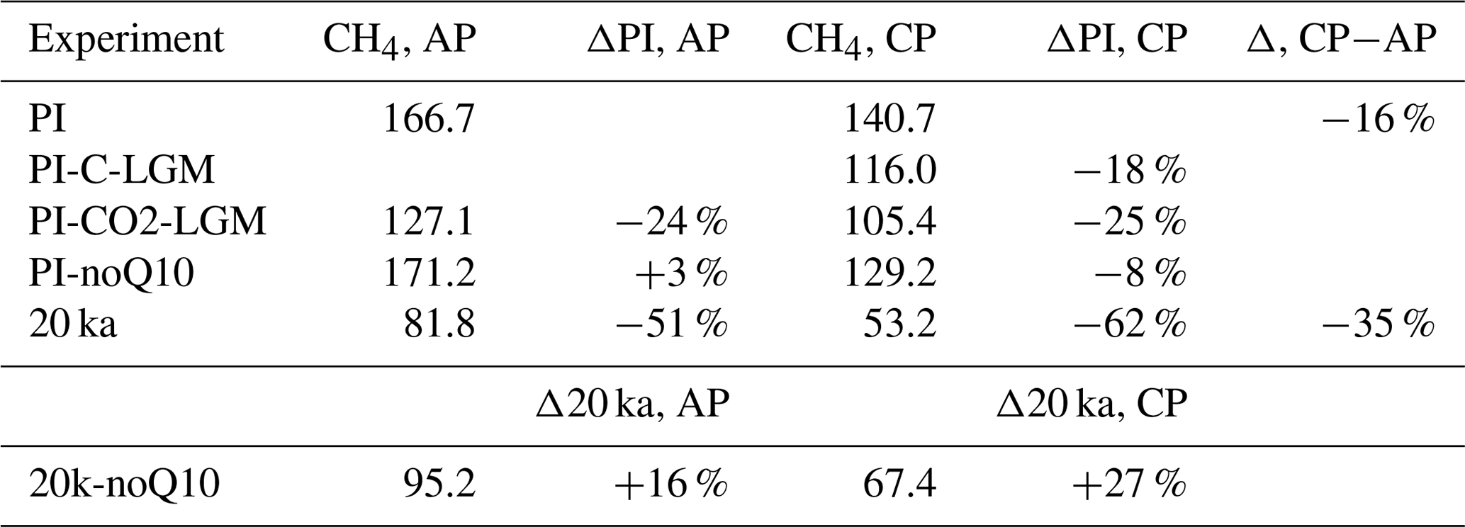
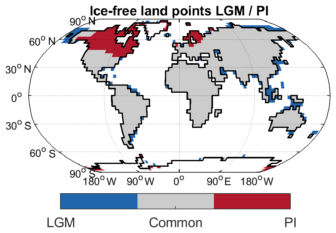
Figure A1 Ice-free land points for LGM and PI time slices, as well as grid points common to both.

Imposing 20 ka land carbon stocks in experiment PI-C-LGM leads to a further reduction by 18 % (evaluated for the common grid points), while imposing 20 ka atmospheric CO₂ for the land biogeochemistry in experiment PI-CO2-LGM leads to a CH₄ emission reduction by 24 % and 25 %, evaluated for all grid points and the common grid points, respectively. The combined effect of 20 ka land carbon and CO₂ is thus a 42 % reduction in emissions (common grid points). The remaining reduction by 20 % of the PI emissions on the common grid points thus needs to be explained by other factors, with temperature change being most important.

Another factor that may be different in our model in comparison to the models previously employed is the temperature dependence of the CO₂-to-CH₄ partitioning during anaerobic decomposition. Disabling this temperature dependence in experiment 20k-noQ10 leads to a 16 % increase in CH₄ emissions, with parameters chosen in such a way that the change is negligible (+3 %) for the PI state. The enabled temperature dependence of the CO₂ to CH₄ partitioning in the standard setup is thus a factor that reduces 20 ka emissions further.

Appendix B: Overview over absolute emissions

For the convenience of readers, who are more interested in absolute emissions than in the differences to the PI state, we also provide an overview over the absolute emissions for the present-day situation (Figs. B1 and B2), as well as the absolute wetland emissions for the past time slices (Fig. B3).

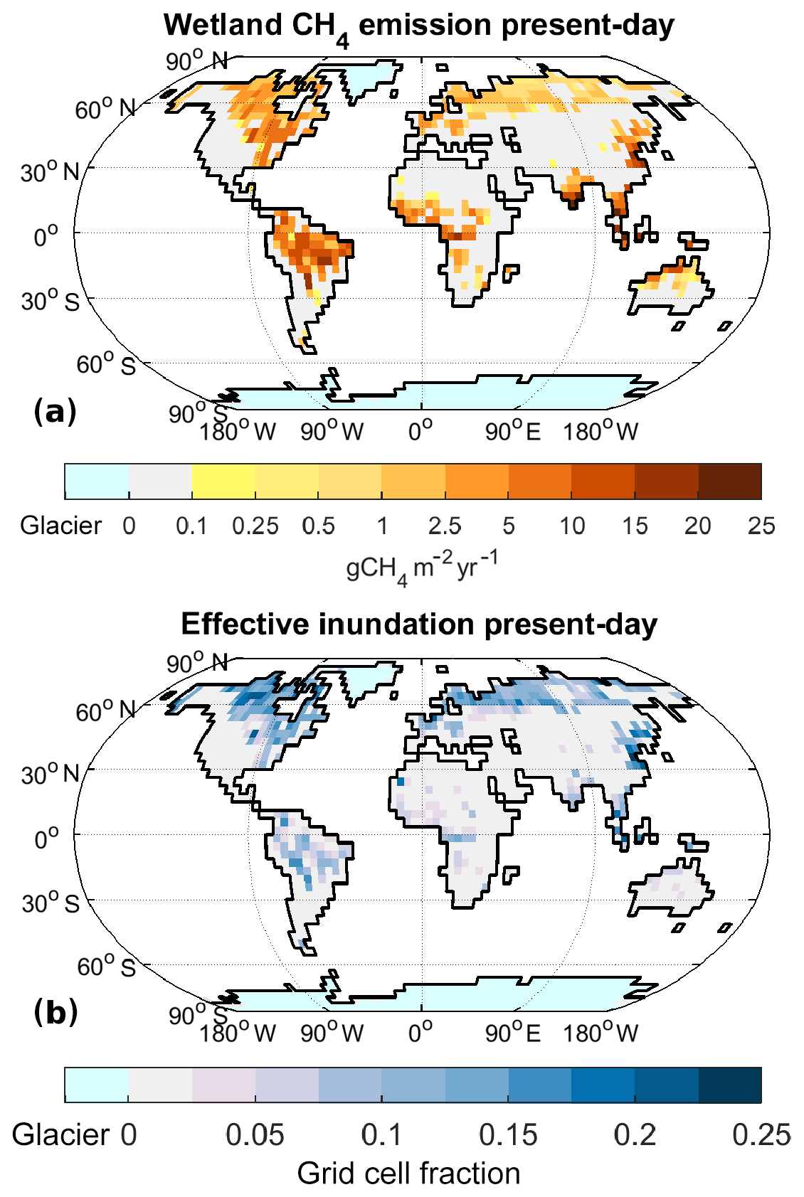
Figure B1 Wetland CH₄ emissions for present-day climate (2000–2009): annual emissions of CH₄ from wetlands (a) and effective inundation (b). Please note the different colour scale for (b) in comparison to Fig. 3.

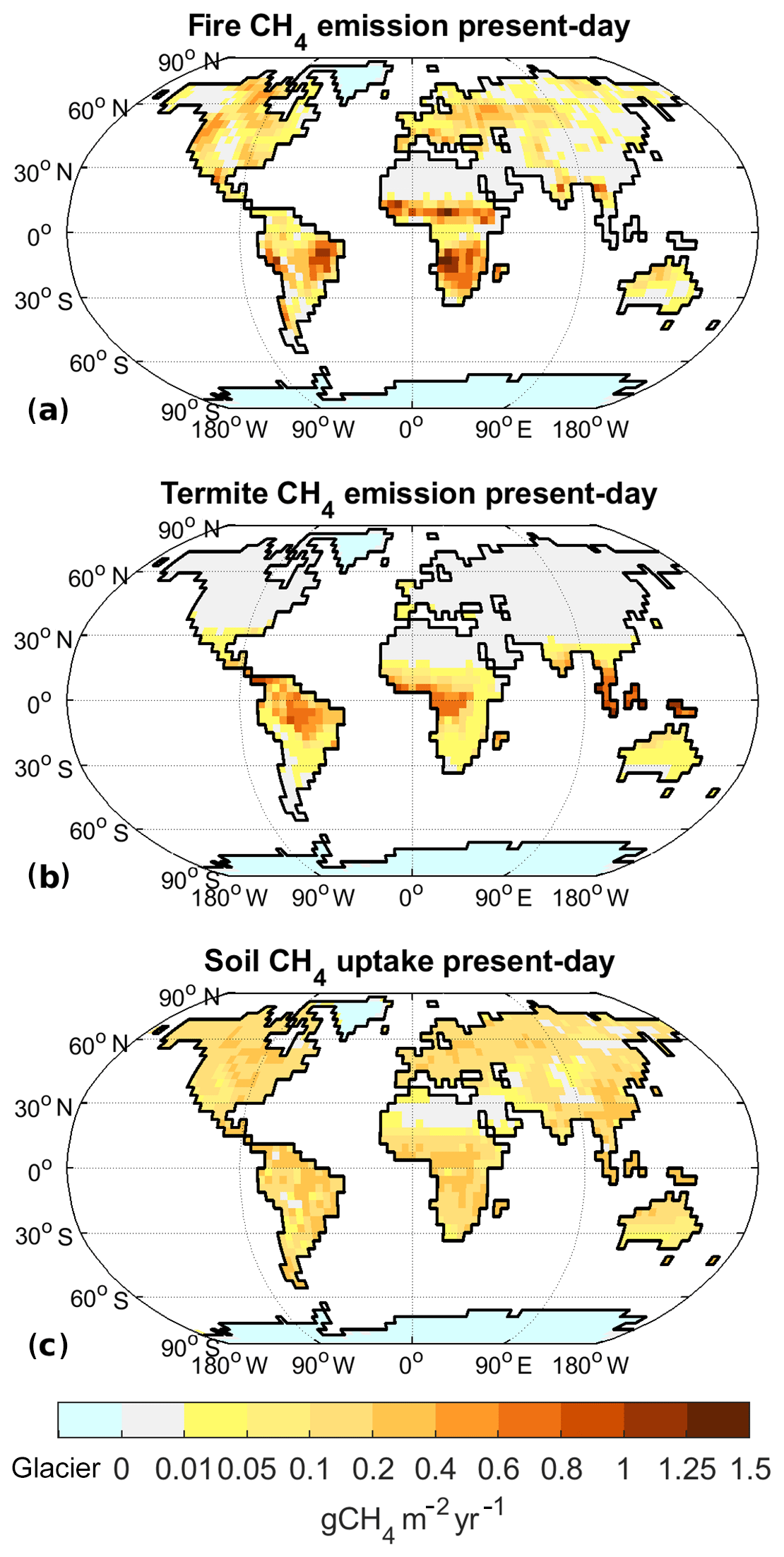
Figure B2 Model results for present-day climate (2000–2009): annual emissions of CH₄ from fires (a), termites (b), and annual soil uptake of CH₄ (c). In comparison to other fluxes, soil uptake has the opposite direction (sign).

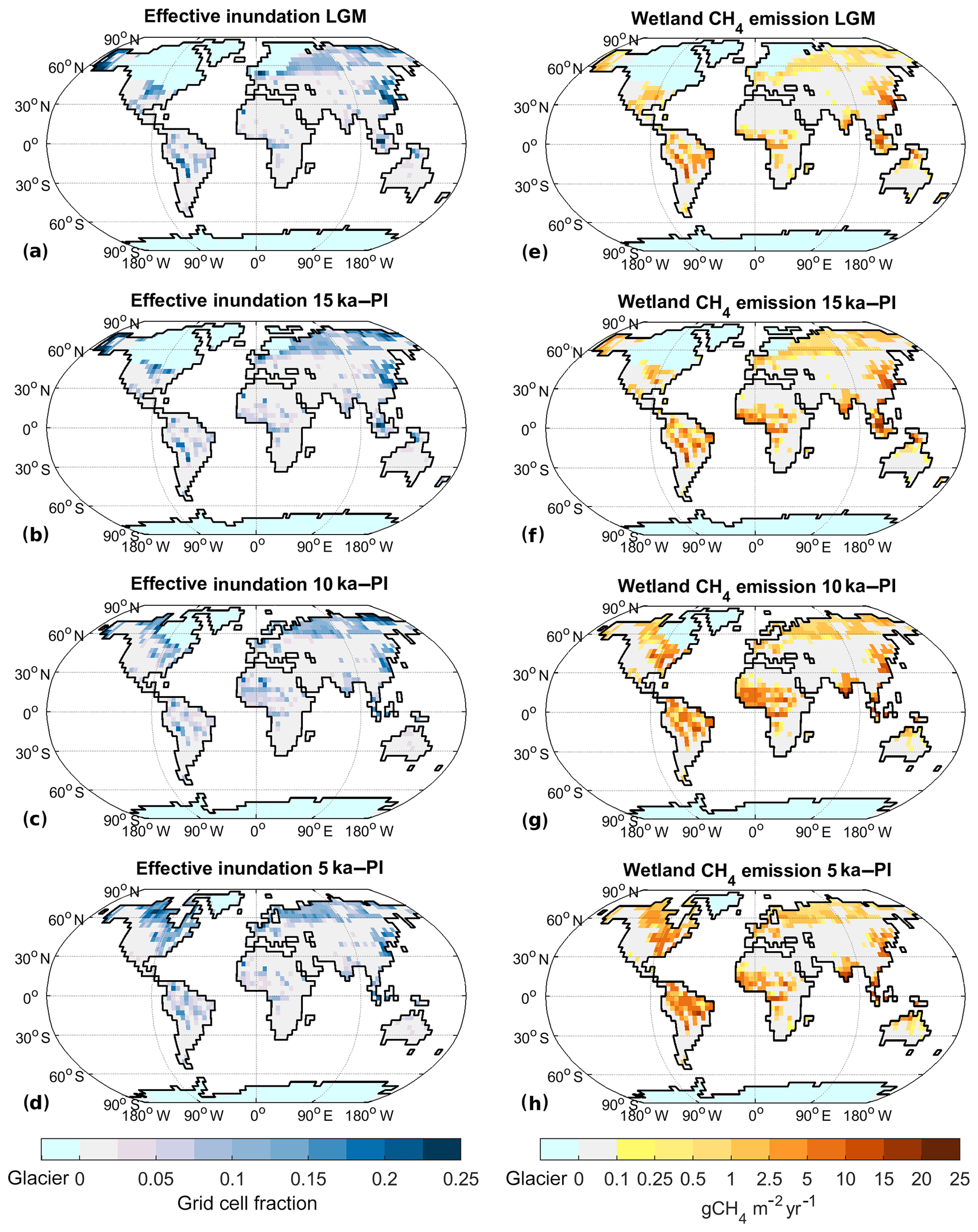
Figure B3 Absolute effective inundation and wetland CH₄ emissions for past climate states: (a–d) effective inundation, (e–h) wetland CH₄ emission. (a, e) LGM, (b, f) 15 ka, (c, g) 10 ka, and (d, h) 5 ka.