Global mean surface temperature and climate sensitivity of the early Eocene Climatic Optimum (EECO), Paleocene–Eocene Thermal Maximum (PETM), and latest Paleocene

Accurate estimates of past global mean surface temperature (GMST) help to contextualise future climate change and are required to estimate the sensitivity of the climate system to CO₂ forcing through Earth's history. Previous GMST estimates for the latest Paleocene and early Eocene (∼57 to 48 million years ago) span a wide range (∼9 to 23 ^∘C higher than pre-industrial) and prevent an accurate assessment of climate sensitivity during this extreme greenhouse climate interval. Using the most recent data compilations, we employ a multi-method experimental framework to calculate GMST during the three DeepMIP target intervals: (1) the latest Paleocene (∼57 Ma), (2) the Paleocene–Eocene Thermal Maximum (PETM; 56 Ma), and (3) the early Eocene Climatic Optimum (EECO; 53.3 to 49.1 Ma). Using six different methodologies, we find that the average GMST estimate (66 % confidence) during the latest Paleocene, PETM, and EECO was 26.3 ^∘C (22.3 to 28.3 ^∘C), 31.6 ^∘C (27.2 to 34.5 ^∘C), and 27.0 ^∘C (23.2 to 29.7 ^∘C), respectively. GMST estimates from the EECO are ∼10 to 16 ^∘C warmer than pre-industrial, higher than the estimate given by the Intergovernmental Panel on Climate Change (IPCC) 5th Assessment Report (9 to 14 ^∘C higher than pre-industrial). Leveraging the large “signal” associated with these extreme warm climates, we combine estimates of GMST and CO₂ from the latest Paleocene, PETM, and EECO to calculate gross estimates of the average climate sensitivity between the early Paleogene and today. We demonstrate that “bulk” equilibrium climate sensitivity (ECS; 66 % confidence) during the latest Paleocene, PETM, and EECO is 4.5 ^∘C (2.4 to 6.8 ^∘C), 3.6 ^∘C (2.3 to 4.7 ^∘C), and 3.1 ^∘C (1.8 to 4.4 ^∘C) per doubling of CO₂. These values are generally similar to those assessed by the IPCC (1.5 to 4.5 ^∘C per doubling CO₂) but appear incompatible with low ECS values (<1.5 per doubling CO₂).

1 Introduction

Under high growth and low mitigation scenarios, atmospheric carbon dioxide (CO₂) could exceed 1000 parts per million (ppm) by the year 2100 (Stocker et al., 2013). The long-term response of the Earth system under such elevated CO₂ concentrations remains uncertain (Stevens et al., 2016; Knutti et al., 2017; Hegerl et al., 2007). One way to better constrain these climate predictions is to examine intervals in the geological past during which greenhouse gas levels were similar to those predicted under future scenarios. This is the rationale behind the Deep-time Model Intercomparison Project (DeepMIP; https://www.deepmip.org/, last access: 21 October 2020) which aims to investigate the behaviour of the Earth system in three high-CO₂ climate states in the latest Paleocene and early Eocene (∼57–48 Ma) (Lunt et al., 2017; Hollis et al., 2019).

Sea surface temperature (SST) and land air temperature (LAT) proxies indicate that the latest Paleocene and early Eocene were characterised by global mean surface temperatures (GMSTs) much warmer than those of today (Cramwinckel et al., 2018; Farnsworth et al., 2019; Hansen et al., 2013; Zhu et al., 2019; Caballero and Huber, 2013). Having a robust quantitative estimate of the magnitude of warming at these times relative to modern is useful for two primary reasons: (1) it allows us to contextualise future climate change predictions by comparing the magnitude of future anthropogenic warming with the magnitude of past natural warming; (2) combined with knowledge of the climate forcing, it allows us to estimate climate sensitivity, a key metric for understanding how the climate system responds to CO₂ forcing. Using different proxy data compilations (Hollis et al., 2012; Lunt et al., 2012), the 5th Intergovernmental Panel on Climate Change (IPCC) Assessment Report (AR5) stated that GMST was 9 to 14 ^∘C higher than for pre-industrial conditions (medium confidence) during the early Eocene (∼52 to 50 Ma) (Masson-Delmotte et al., 2014). However, subsequent studies indicate a wider range of estimates, from 9 to 23 ^∘C warmer than pre-industrial (Caballero and Huber, 2013; Cramwinckel et al., 2018; Farnsworth et al., 2019; Zhu et al., 2019; Fig. 1 and Table 1). It is an open question whether this range arises from inconsistencies between the methods used to estimate GMST, such as selection of proxy datasets, treatment of uncertainty, and/or analysis of different time intervals. This methodological variability has thwarted robust comparisons between GMST methodologies for key intervals through the latest Paleocene to early Eocene.

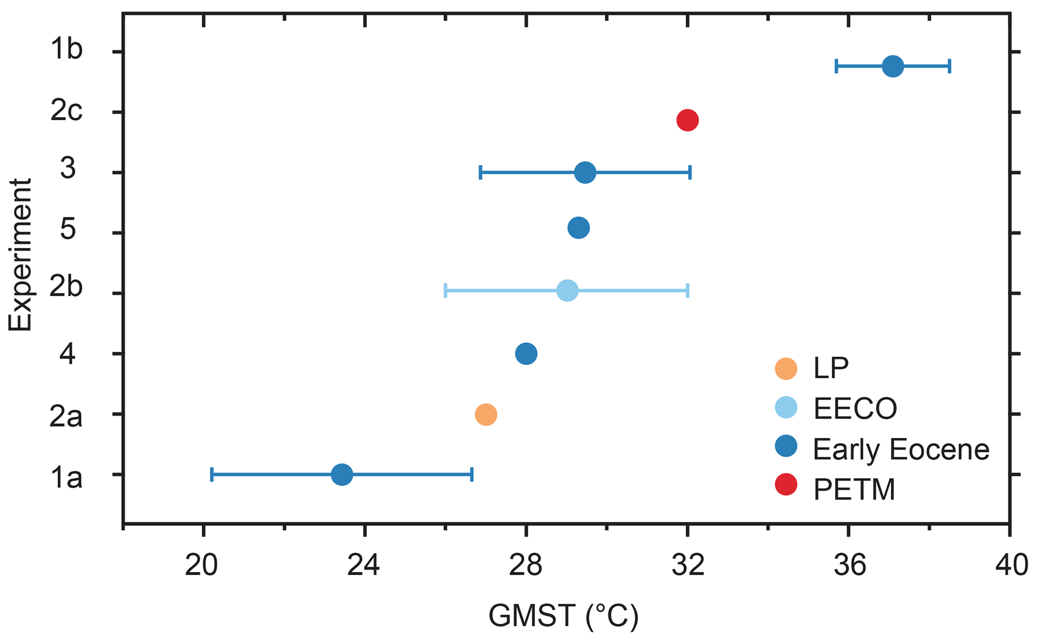
Figure 1 Published GMST estimates during the early Paleogene (57 to 48 Ma). Dots represent average values. The horizontal limits on the individual dots represent the reported error, and y-axis labels refer to previous estimates (see Table 1).

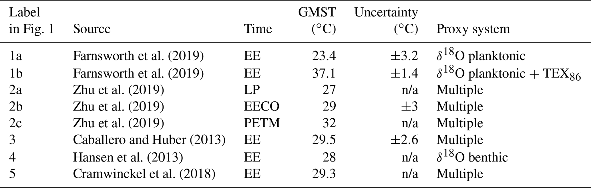
Table 1 Previous studies that have determined GMST for the early Eocene (EE), EECO, PETM, or latest Paleocene (LP); n/a indicates that no error bars were reported in the original publications.

Here we calculate GMST estimates within a consistent experimental framework for the target intervals outlined by DeepMIP: (i) the Early Eocene Climatic Optimum (EECO; 53.3 to 49.1 Ma), (ii) the Paleocene–Eocene Thermal Maximum (PETM; ca. 56 Ma), and (iii) the latest Paleocene (LP; ca. 57–56 Ma). We use six different methods to obtain new GMST estimates for these three time intervals by employing previously compiled SST and LAT estimates (Hollis et al., 2019) as well as bottom water temperature (BWT) estimates (Dunkley Jones et al., 2013; Cramer et al., 2009; Sexton et al., 2011; Littler et al., 2014; Laurentano et al., 2015; Westerhold et al., 2018; Barnet et al., 2019). We also undertake a suite of additional sensitivity studies to explore the influence of particular proxies on each GMST estimate. We then compile GMST estimates from all six methods to generate a “combined” GMST estimate for each time slice and use these, with existing estimates of CO₂ (Gutjahr et al., 2017; Anagnostou et al., 2016), to develop new estimates of “bulk” equilibrium climate sensitivity (ECS) during the latest Paleocene, PETM, and EECO.

2 Methods and materials

Three different input datasets are used to calculate GMST: (1) dataset D_surf, which consists of surface temperature estimates, both marine (sea surface temperature) and terrestrial, (2) dataset D_deep, which consists of deep-water temperature estimates, and (3) dataset D_comb, which consists of a combination of surface- and deep-water temperature estimates. Here we make use of six different methodologies, which are described in detail below, to estimate GMST from these datasets.

2.1 Dataset D_surf

Dataset D_surf is version 0.1 of the DeepMIP database, as described in Hollis et al. (2019) (Supplement). It consists of SSTs and LATs for the latest Paleocene, PETM, and EECO. The SSTs are derived from foraminiferal δ¹⁸O values, foraminiferal Mg∕Ca ratios, clumped isotopes (Δ47), and isoprenoid glycerol dialkyl glycerol tetraethers (GDGTs) (TEX₈₆). Foraminiferal δ¹⁸O values and Mg∕Ca ratios are calibrated to SST following Hollis et al. (2019) and Evans et al. (2018), respectively. TEX₈₆ values are calibrated to SST using BAYSPAR (Tierney and Tingley, 2014). Δ47 values are reported using the parameters and calibrations of the original publications (Evans et al., 2018; Keating-Bitonti et al., 2011). LATs are derived from leaf fossils, pollen assemblages, mammal δ¹⁸O values, paleosol δ¹⁸O values, paleosol climofunctions, and branched GDGTs. LAT estimates are calculated using the parameters and calibrations of the original publications (see Hollis et al., 2019, and references therein). The locations of the proxy datasets are shown in Fig. S1 in the Supplement using the paleomagnetic-based reference frame (Hollis et al., 2019). For each dataset, we utilise the uncertainty range of temperature estimates reported in Hollis et al. (2019).

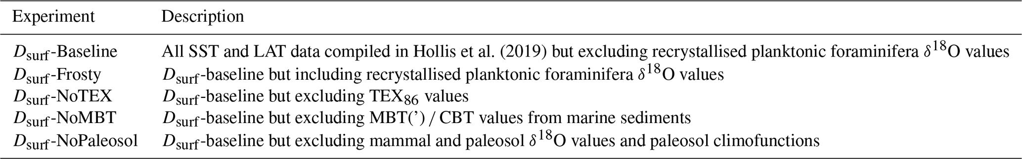
Four methods (D_surf-1, D_surf-2, D_surf-3, and D_surf-4) are employed to calculate GMST from dataset D_surf. These methods employ parametric (D_surf-1, D_surf-2, D_surf-4) or non-parametric (D_surf-3) functions to estimate temperature. We calculate GMST on the mantle-based reference frame and employ the rotations provided in Hollis et al. (2019). These differ very slightly from those utilised in the DeepMIP model simulations (Lunt et al., 2020). Each method conducts a “baseline” calculation that uses the SST and LAT data compiled in accordance with the DeepMIP protocols (i.e. Hollis et al., 2019). Our baseline calculation (D_surf-baseline; Table 2) excludes δ¹⁸O values from recrystallised planktonic foraminifera because the resulting temperature estimates are biased by diagenesis toward significantly cooler temperatures than those derived from (i) the δ¹⁸O value of similarly aged and similarly located well-preserved foraminifera, (ii) foraminiferal Mg∕Ca ratios, and (iii) Δ47 values from larger benthic foraminifera (Pearson et al., 2001; Hollis et al., 2019, and references therein). For each method, we also conduct a series of illustrative subsampling calculations relative to D_surf-baseline based on varying assumptions about the robustness of different proxies (Table 2). The first sensitivity experiment (D_surf-Frosty; Table 2) includes δ¹⁸O values from recrystallised planktonic foraminifera. The second sensitivity experiment (D_surf-NoTEX; Table 2) removes TEX₈₆ values as these give slightly higher SSTs than other proxies, especially in the middle to high latitudes (Bijl et al., 2009; Hollis et al., 2012; Inglis et al., 2015). The third sensitivity experiment (D_surf-NoMBT; Table 2) removes MBT(') ∕ CBT values derived from marine sediment archives as they may suffer from a cool bias (Inglis et al., 2017; Hollis et al., 2019). The fourth sensitivity experiment (D_surf-NoPaleosol; Table 2) removes mammal and paleosol δ¹⁸O values as well as paleosol climofunctions as these proxies may suffer from a cool bias (Hyland and Sheldon, 2013; Hollis et al., 2019). For each method, GMST is calculated for (i) the Early Eocene Climatic Optimum (EECO; 53.3 to 49.1 Ma), (ii) the Paleocene–Eocene Thermal Maximum (ca. 56 Ma), and (iii) the latest Paleocene (LP; ca. 57–56 Ma).

Table 2 Baseline and optional subsampling experiments applied to D_surf.

2.1.1 D_surf-1

Method D_surf-1 was first employed by Caballero and Huber (2013) to estimate GMST from early Eocene surface temperature proxies after it was recognised that pervasive recrystallisation of foraminiferal δ¹⁸O could overprint the original SST signal (e.g. Pearson et al., 2001, 2007). That study used data compilations (Huber and Caballero, 2011; Hollis et al., 2012) which were the predecessors to the DeepMIP compilation (Hollis et al., 2019).

Here, the anomalies of individual proxy temperature data points with respect to modern values at the corresponding paleolocation are first calculated. The time period used is between 1979 and 2018, and we used a climatology of the full ERA-Interim period (Dee et al., 2011). The calculation involves binning into low, middle, and high latitudes (30^∘ N to 30^∘ S, 30 to 60^∘ N–S, and 60 to 90^∘ N–S) and calculating the unweighted mean anomaly within these bins between the median reconstructed value at a given locality and the temperature in the modern system (from reanalysis). The geographically binned means are then weighted according to relative spherical area to calculate a globally weighted mean temperature anomaly between the paleo-time slice and modern. All samples are treated equally and considered independent. The associated errors are added in quadrature with the inter-sample standard deviation. These two sources of error were combined and normalised by the square root of the number of samples. This method is intended as an unsophisticated, brute-force approach to estimating GMST when dealing with many localities with poorly characterised errors in which there is a large difference between the reconstructed temperature at a given location and the modern equivalent. It is not intended to identify small changes in GMST; nor is it expected to work well under conditions in which temperature gradients are stronger than today, continents are far removed from their current configuration, or systematic errors are not readily mitigated by large sample size (i.e. when there are correlations in systematic errors between proxies). It is designed to be relatively straightforward to interpret and simple to reproduce without overly relying on climate models or sophisticated statistical models.

Various sanity checks have been performed to determine if the method is likely to produce useful results for a given sampling distribution and what corrections should be applied to optimise it. For example, if the modern temperature field is sampled using a geographic sampling distribution for a given time interval, what would the reconstructed modern temperature be? Sampling the modern global annual average surface temperature field in the reanalysis product ERA-5 yields a mean value of 15.1 ^∘C, but when resampled at the equivalent geographic distribution of our samples from the latest Paleocene, PETM, and EECO yields mean values for the modern of 16.9 ^∘C (±1.8 ^∘C), 14.2 ^∘C (±1.7 ^∘C), and 15.2 ^∘C (±1.1 ^∘C), respectively. Thus, for the sampling densities and spatial structure of the early Paleogene, this method can approach the true value within ∼1.5 ^∘C and the error propagation adequately characterises the error in this “perfect knowledge” scenario. Seeking precision beyond that range is unwarranted and, as indicated above, systematic biases are a serious concern. However, estimating the latest Paleocene and early Eocene GMST may be somewhat easier than estimating the modern GMST because temperature gradients were greatly reduced compared to modern. Huber and Caballero (2011) estimate a reduction to less than half the modern temperature gradient, whilst Evans et al. (2018) constrain the low- to high-latitude SST gradient to at least ∼30 % (±10 %) weaker than modern (Evans et al., 2018).

Alongside modern observations, we can also use paleoclimate model results to characterise how well the existing paleogeographic sampling network will impact results (Fig. 2). Here we utilise two CESM1 simulations, as described in Cramwinckel et al. (2018; EO3 and EO4). The two cases are chosen to minimise the magnitude of the correction to GMST, and the final result is not sensitive to the choice of reference simulation between these two (Supplement). For each interval, the difference between reconstructed global temperatures and the true paleoclimate model mean is <1 to 3 ^∘C. These comparisons demonstrate that this method produces estimates that are within random error given otherwise perfect knowledge. The errors introduced by limited paleogeographic sampling can be alleviated by incorporating the offset in mean values between the true paleoclimate model GMST and the sampled paleoclimate model GMST outlined above (Fig. 2). We utilise this offset to correct for systematic errors, but this is the only component in which paleoclimate model information is included in this GMST estimation methodology. This approach is best applied within the context of studying the random and systematic error structure as described above, and caution should be taken in using systematic corrections that are significantly bigger than the estimated random error. The underlying assumption is that the bias in the global mean estimate that exists due to uneven sampling is the same in the “proxy” Eocene world as in the “model” Eocene world, i.e. that the zonal and meridional gradients are well characterised by the model, even if the absolute temperatures are not.

Figure 2 An illustration of method D_surf-1 during the EECO. (a) Modelled early Eocene temperatures utilising CESM1.2 at 6× pre-industrial CO₂, (b) interpolated absolute SST reconstructions, and (c) data–model difference between (a) and (b).

We note that the magnitude of the global correction could be sensitive to different models and/or boundary conditions. To explore this further, we performed the same analysis using Community Earth System Model version 1.2 (CESM1.2) at 6×CO₂. This model simulation offers a major improvement over earlier models (Zhu et al., 2019) due to the improved treatment of cloud microphysics and is able to reproduce key features of the early Paleogene (e.g. the meridional SST gradient; Zhu et al., 2019; Lunt et al., 2020). We find that CESM1 (8× and 16×CO₂) and CESM1.2 (6×CO₂) yield similar GMST estimates during the PETM, EECO, and latest Paleocene. For example, GMST values (obtained using D_surf-baseline) during the EECO average 24.5, 24.6, and 25.2 ^∘C for CESM1 (×8 CO₂), CESM1 (×16 CO₂), and CESM1.2 (6×CO₂), respectively. This indicates that the final result is not overly sensitive to the choice of reference simulation, at least within the CESM family. In the following sections, we only discuss CESM1 simulations to avoid circularity if the results from this paper are used to evaluate more recent simulations (e.g. CESM1.2; Lunt et al., 2020).

2.1.2 D_surf-2

GMST estimates are calculated using the method described in Farnsworth et al. (2019), in which a transfer function is used to calculate global mean temperature from local proxy temperatures. The transfer function is generated from a pair of early Eocene climate model simulations carried out at two CO₂ concentrations. The first simulations are the same 2×CO₂ and 4×CO₂ HadCM3L Eocene simulations from Farnsworth et al. (2019). The second simulations are the 4×CO₂ and 8×CO₂ CCSM3 simulations of Huber and Caballero (2011), also discussed in Lunt et al. (2012). The two models are configured for the Eocene with different paleogeographies (Table S1 in the Supplement). We provide a final estimate based on the mean of our two models.

The principal assumption of this approach is that global temperatures scale linearly with local temperatures and that a climate model can represent this scaling correctly (see below). The resulting GMST estimate is therefore independent of the climate sensitivity of the model but dependent on the modelled spatial distribution of temperature. For a single given proxy location with a local temperature estimate (T^proxy), Farnsworth et al. (2019) estimate global GMST ($<T{>}^{\mathrm{inferred}})$ as

$$\begin{array}{}\text{(1)}& \begin{array}{rl}<T{>}^{\mathrm{inferred}}& =<T^{\mathrm{low}}>\\ & +\left(T^{\mathrm{proxy}}{T}^{\mathrm{low}}\right){\displaystyle \frac{<T^{\mathrm{high}}>-<T^{\mathrm{low}}>}{T^{\mathrm{high}}-T^{\mathrm{low}}}},\end{array}\end{array}$$

where $<T^{\mathrm{low}}>$ and $<T^{\mathrm{high}}>$ are the global means of a low- and high-CO₂ model simulation, respectively, and T^low and T^high are the local temperatures (same location as the proxy) from the same simulations. T^lowand T^high represent local modelled SSTs or local modelled near-surface LATs (in contrast to Farnsworth et al. 2019, who only used local modelled near-surface LATs to calculate T^low and T^high, even if T^proxy was SST). If the proxy temperature is greater than T^high or cooler than T^low, then the inferred global mean is found by extrapolation rather than by interpolation and is therefore more uncertain (Fig. 3). This will be sensitive to the choice of model simulation; models that simulate less polar amplification (e.g. HadCM3L) are more likely to obtain $<T{>}^{\mathrm{inferred}}$ (i.e. GMST) via extrapolation. We repeat this process for each proxy data location (Fig. 4) and take an average over all proxy locations as our best estimate of global mean temperature.

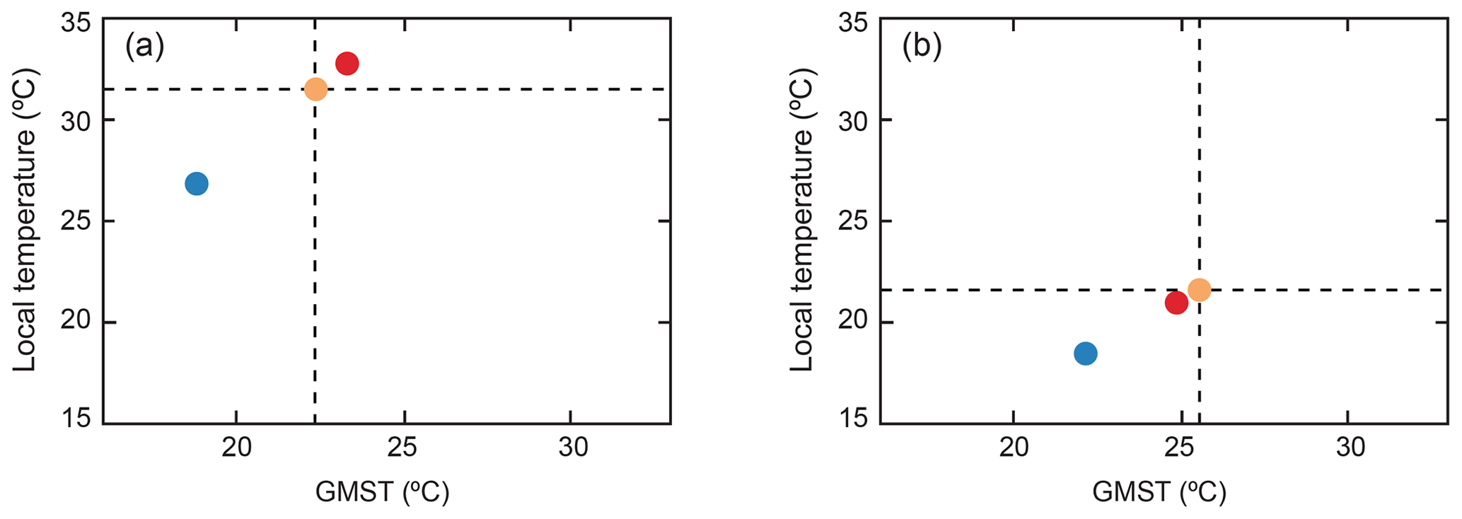
Figure 3 An illustration of method D_surf-2 for two sites: (a) Big Bend LAT in the EECO as diagnosed using HadCM3L and (b) DSDP Site 401 SST in the PETM as diagnosed using CCSM3. The vertical dashed line shows $<T{>}^{\mathrm{inferred}}$ and the horizontal dashed line shows T^proxy, which intercept at the orange dot. The dark blue dots show the intercept of T^low with $<T^{\mathrm{low}}>$, and the red dots show the intercept of T^high with $<T^{\mathrm{high}}>$.

Figure 4 Inferred global mean temperature ($<T{>}^{\mathrm{inferred}})$ using D_surf-2 for (a) each EECO-aged LAT proxy as diagnosed using HadCM3L and (b) each PETM-aged SST proxy as diagnosed using CCSM3. For (a) and (b), the final estimate of global mean temperature is the average of all the individual sites. The solid line shows the continental outline in each model, and the dashed line shows the continental outline.

Recent work has demonstrated that CESM1.2 and GFDL model simulations offer a major improvement over earlier models (Zhu et al., 2019; Lunt et al., 2020). As such, we also calculated GMST using CESM1.2 (3× and 6×CO₂; Zhu et al., 2019; Table S1) and GFDL (3× and 6×CO₂; Hutchinson et al., 2018; Lunt et al., 2020; Table S1). We find that all four simulations (i.e. HadCM3L, CCSM3, CESM1.2, and GFDL) yield similar GMST estimates. For example, GMST during the PETM ranges between 32.3 and 34.5 ^∘C (Supplement). This demonstrates that D_surf-2 is not overly sensitive to the climate model simulation. However, as CESM1.2 and GFDL have greater polar amplification than other models (e.g. HadCM3L), GMST is more likely to be found by interpolation (compare to extrapolation). To explore whether GMST scales linearly with local temperatures, we used CESM1.2 to recalculate GMST using the same method as above but using the 9×CO₂ simulation in place of the 6×CO₂ simulation. We find that GMST estimates are very similar (±0.4 ^∘C). This is because, although the relationship between GMST and CO₂ is non-linear (Zhu et al., 2019), the relationship between local and global temperature is relatively constant. In the following sections, we employ CCSM3 and HadCM3 simulations to avoid circularity if the results from this paper are used to evaluate more recent simulations (e.g. CESM1.2, GFDL; Lunt et al., 2020).

2.1.3 D_surf-3

For D_surf-3, GMST estimates are calculated using Gaussian process regression (Fig. 5; Bragg et al., 2020). In this method, temperature is treated as an unknown function of location, f(x). Many possible functions can fit the available proxy dataset. By using a Gaussian process model of the unknown function, we assume that temperature is a continuous and smoothly varying function of location, and once fitted to the data, the posterior mean of the model gives the most likely function form for the temperature. We use a Gaussian process prior and update it using the proxy data to obtain the posterior model, which we can then use to predict the surface temperatures on a global grid. Prior specification of the model is via a mean function E(f(x))=m(x) and a covariance function Cov$\left(f\right(x),f(x^{\prime }\left)\right)=k(x,x^{\prime })$ (which tells us how correlated f(x) is with f(x^′)). We also specify the standard deviation of the observation uncertainty about each data point (${\mathit{\sigma }}_i^{\mathrm{2}})$. If $\mathit{f}={\left(f\left(x_{\mathrm{1}}\right),\mathrm{\dots }f\left(x_n\right)\right)}^T$ is a vector of temperature observations at each location x_i, then the model is

$$\begin{array}{}\text{(2)}& \mathit{f}\sim N(\mathit{\mu },\mathrm{\Sigma }),\end{array}$$

where μ_i=m(x_i) and ${\mathrm{\Sigma }}_{ij}=k\left(x_i,x_j\right)+I_{i=j}{\mathit{\sigma }}_i^{\mathrm{2}}$. The proxy temperatures are expressed as anomalies to either the marine or terrestrial present-day zonal mean temperature at the respective paleolatitude. We subtract the mean temperature anomaly (weighted by the paleolatitude) for each time period and core experiment prior to the analysis and therefore fit the model to the residuals. This means the predicted field will relax towards the mean surface warming in areas of no data coverage. The covariance function – which considers the clustering of proxy locations – describes the correlation between f(x_i) and f(x_j) in relation to the distance of x_i and x_j. We use a squared-exponential covariance function with Haversine distances replacing Euclidean distances so that correlation is a function of distance on the sphere.

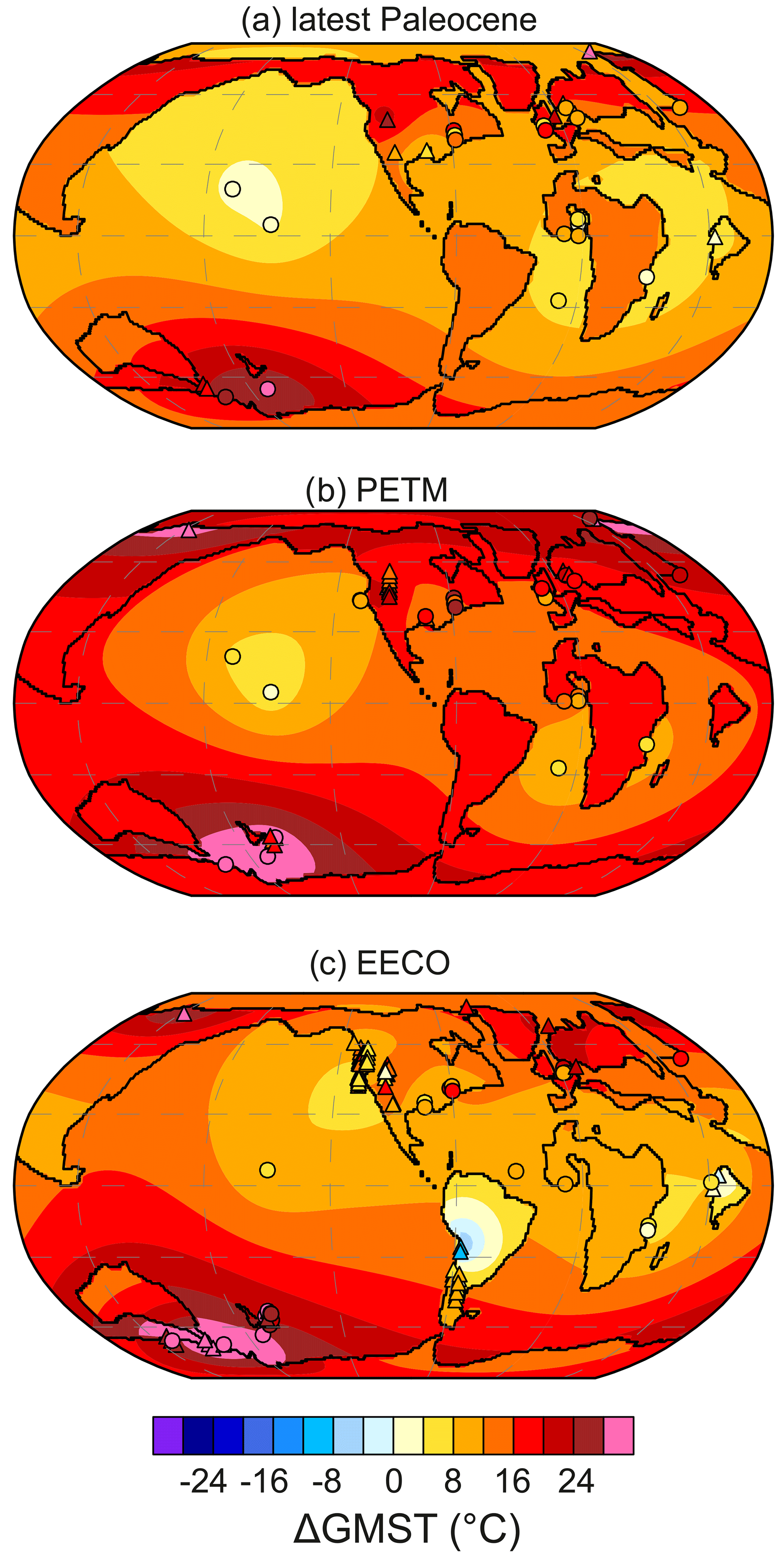
Figure 5 Predicted surface warming by Gaussian process regression using D_surf-3 for the (a) latest Paleocene, (b) PETM, and (c) EECO. Anomalies are relative to the present-day zonal mean surface temperature. Circles (triangles) indicate all available SST (LAT) proxy data for the respective time slice used to train the model. Symbols for locations where multiple proxy reconstructions are available are slightly shifted in latitude for improved visibility.

A heteroscedastic noise model is used to weight the influence of individual proxy data by their associated uncertainty; i.e. the model will better fit reconstructions with a smaller reported error. Proxy uncertainties are taken from Hollis et al. (2019). Standard deviations for TEX₈₆, Mg∕Ca, and δ¹⁸O records are derived from the reported 90 % confidence intervals (Hollis et al., 2019). A minimum value of 2.5 ^∘C for the standard deviation is assumed for all other methods. The output variances and length scale of the covariance function are estimated using their maximum likelihood values, obtained with the GPy Python package (GPy, 2012). We apply the method to the marine and terrestrial data separately and combine the masked fields afterwards to prevent mutual interference. We further constrain the lower bound of the length scale parameter to 2000 km to always fit a reasonably smooth surface, even in some continental areas with noisy proxy data (e.g. western North America). We note that our choice of the minimum length scale and the separation of land and ocean temperatures influence the predicted regional surface temperature patterns but do not significantly change our GMST estimates.

The Gaussian process approach provides probabilistic predictions of temperature values, i.e. uncertainty estimates of the predicted field. The uncertainty reported for an individual GMST estimate is calculated via random sampling. We generate 10 000 surfaces from a multivariate normal distribution based on the predicted mean and full covariance matrix and calculate the GMST for each sample. Uncertainty of the mean estimate is then defined as the standard deviation of the 10 000 random samples. Regional model uncertainty (expressed as standard deviation fields) is typically highest in areas with sparse data coverage (e.g. the Pacific Ocean and Southern Hemisphere landmasses; Fig. S2). The lower uncertainty for the latest Paleocene relative to the PETM and EECO is related to the smaller reported uncertainties in the proxy dataset rather than enhanced data coverage. The large spread in reconstructed terrestrial temperatures for North America during the PETM and EECO (Fig. S2) propagates through into relatively large uncertainties in the GMST estimates for these intervals.

2.1.4 D_surf-4

For D_surf-4, GMST estimates are calculated using a simple function of latitude (θ) tuned to best fit the proxy data:

$$\begin{array}{}\text{(3)}& T\left(\mathit{\theta }\right)\approx a+b\mathit{\theta }+c\cos \mathit{\theta },\end{array}$$

where T(θ) is the Eocene zonal mean temperature, and the coefficients a, b, and c are chosen to minimise the sum of the squared residuals relative to D_surf (i.e. the SST and LAT data from Hollis et al., 2019). This new model represents T(θ) well in the modern climate (Fig. S3) when supplied with a similar number of data points as in the Hollis et al. (2019) dataset, and it ensures a global solution that is consistent with the physical expectation that temperature should decrease – and the meridional gradient in temperature should increase – from the tropics toward the poles (Fig. S3).

For each data point, we account for three types of uncertainty (i.e. temperature, elevation, latitude). For temperature, we assume a skew-normal probability distribution based on the stated 90 % confidence intervals. Where uncertainty estimates are not given, we assume a (symmetric) normal distribution with a 90 % confidence interval of ±5 K. For elevation, we assume a skew-normal distribution with a 90 % confidence interval equal to the lowest and highest elevations of adjacent grid points in the paleotopography dataset of Herold et al. (2014), with a lower bound of zero.

T(θ) was estimated by sampling temperature, elevation, and latitude from their respective distributions at each location (Fig. S4), and a lapse-rate adjustment of 6^∘ K km⁻¹ was applied. Then, using a standard Monte Carlo bootstrapping method, the same number of data points was resampled via replacement, and the coefficients in Eq. (3) were found that best fit the subsampled data. This procedure was repeated 10 000 times to find a probability distribution of T(θ). The uncertainty associated with an individual GMST estimate is the standard deviation.

2.2 Dataset D_deep

Dataset D_deep consists of benthic foraminiferal δ¹⁸O-derived bottom water temperatures (BWTs) for the latest Paleocene, PETM, and EECO. The benthic foraminiferal δ¹⁸O dataset is based on previous compilations (Dunkley Jones et al., 2013; Cramer et al., 2009), updated to include more recently published datasets (Sexton et al., 2011; Littler et al., 2014; Laurentano et al., 2015; Westerhold et al., 2018; Barnet et al., 2019). The EECO dataset is sourced from 11 sites, providing spatial coverage of the Pacific, Atlantic, and Indian Ocean (DSDP/ODP Sites 401, 550, 577, 690, 702, 738, 865, 1209, 1258, 1262, and 1263). The PETM and latest Paleocene datasets are sourced from a compilation of nine and seven sites, respectively, differing from Dunkley-Jones et al. (2013) in that (i) more recent datasets were added, and (ii) PETM sites with a muted carbon isotope excursion (CIE) magnitude (<1.5 ‰) were excluded as these datasets may be missing the core PETM interval (Table S2). Benthic foraminifera δ¹⁸O values are adjusted to Cibicidoides following established methods (Cramer et al., 2009), allowing temperature to be calculated using Eq. (9) of Marchitto et al. (2014):

$$\begin{array}{}\text{(4)}& \begin{array}{rl}({\mathit{\delta }}_{\mathrm{cp}}-{\mathit{\delta }}_{\mathrm{sw}}+\mathrm{0.27})& =-\mathrm{0.245}\pm \mathrm{0.005}t+\mathrm{0.0011}\\ & \pm \mathrm{0.0002}{t}^{\mathrm{2}}+\mathrm{3.58}\pm \mathrm{0.02},\end{array}\end{array}$$

where t is bottom water temperature in Celsius, δ_cp is δ¹⁸O of CaCO₃ on the Vienna Pee Dee Belemnite (VPDB) scale, and δ_sw is δ¹⁸O of seawater on the Standard Mean Ocean Water (SMOW). δ_sw is defined in accordance with the DeepMIP protocols (−1.00 ‰; see Hollis et al., 2019).

2.2.1 D_deep-1

For D_deep-1, GMST estimates are calculated following the method of Hansen et al. (2013), which utilises only the deep-ocean benthic foraminifera δ¹⁸O dataset, and we refer the reader to that study for a detailed justification of the approach. Briefly, for time periods prior to the Pliocene, GMST is scaled directly to deep-ocean temperature. Specifically, ΔGMST = ΔBWT prior to ∼5.3 Ma, with early Pliocene BWT and GMST calculated following Eqs. (3.5), (3.6), and (4.2) of Hansen et al. (2013). As such, the calculations presented here differ from those of Hansen et al. (2013) only in that (i) we use the revised benthic δ¹⁸O compilation described above rather than that of Zachos et al. (2008) and (ii) a different equation (Eq. 4) to convert δ¹⁸O to temperature.

2.3 Dataset D_comb

Dataset D_comb uses a combination of (tropical) surface- and deep-water temperature estimates. The deep-ocean dataset (D_deep) is identical to that described in Sect. 2.2. The tropical SST dataset utilises all relevant surface-ocean proxy data from the DeepMIP database, i.e. those with a paleolatitude in the magnetic reference frame within 30^∘ of the Equator. An expanded (relative to modern) definition of the tropics is used because tropical SST reconstructions are relatively sparse; 30^∘ was chosen because it retains tropical SST data from several proxies for all three intervals, whilst SST seasonality remains relatively low within these latitudinal bounds.

2.3.1 D_comb-1

For D_comb-1, GMST estimates are calculated for each time interval based on the difference between tropical SSTs and deep-ocean BWTs (Evans et al., 2018) such that

$$\begin{array}{}\text{(5)}& \mathrm{GMST}=\mathrm{0.5}(\stackrel{\mathrm{‾}}{\mathrm{tropical}\mathrm{SST}}+\stackrel{\mathrm{‾}}{\mathrm{BWT}}).\end{array}$$

The fundamental assumptions of this approach are that (1) GMST can be approximated by global mean SST, (2) global mean SST is equivalent to the mean of the tropical and high-latitude regions, (3) benthic temperatures are representative of high-latitude surface temperatures, and (4) the temperature gradient between the abyss and high-latitude SST is fixed through time (see Sijp et al., 2011). To test these assumptions from a theoretical perspective, we modelled the shape of the latitudinal temperature gradient using a simple algebraic function (Fig. S5). These results suggest that D_comb-1 may underestimate GMST by 0.75 to 1.25 ^∘C in the modern. We also compared GMST from the EO3 and EO4 model simulations of Cramwinckel et al. (2018) to that calculated using D_comb-1 (Fig. S5) and find a similar cold bias during the Eocene (∼1 to 3 ^∘C). However, we note that these findings depend on the accuracy of the modelled deep-ocean temperatures.

Probability distributions for each time interval were computed as follows. In the case of the tropical SST data, 1000 subsamples were taken, following which a random normally distributed error was added to each data point in the DeepMIP compilation, including both calibration uncertainty and variance in the data where multiple reconstructions are available for a given site and time interval. Mean tropical SST was calculated for each of these subsamples. To provide a BWT dataset of the same size as the subsampled tropical SST data, 1000 normally distributed values were calculated for each time interval based on the mean ±1 SD variation of the pooled benthic δ¹⁸O data from all sites including calibration uncertainty.

3 Results and discussion

3.1 Comparison of surface and bottom water temperature-derived GMST estimates

The following section discusses our baseline GMST estimates calculated on the mantle-based reference frame only. During the latest Paleocene and PETM, GMST estimates derived from D_surf-baseline average ∼27 and 33 ^∘C, respectively (Table 3; Fig. 6). These values are consistent with previous studies analysing the latest Paleocene (∼27 ^∘C; Zhu et al., 2019) and PETM (∼32 ^∘C; Zhu et al., 2019). During the EECO, GMST estimates calculated using D_surf average ∼27 ^∘C (Fig. 6). These values are up to 3 ^∘C lower compared to previous estimates from similar time intervals (ca. 29 to 30 ^∘C; Huber and Caballero, 2011; Caballero and Huber, 2013; Zhu et al., 2019). This is likely because we use an expanded LAT dataset (n=80) compared to previous studies (n=51; Huber and Caballero, 2011). Several of these proxies saturate between ∼25 and 29 ^∘C (e.g. leaf fossils, pollen assemblages, and brGDGTs; see Hollis et al., 2019, and references therein) and/or are impacted by non-temperature controls (e.g. paleosol climofunctions; see below) and could skew GMST estimates towards lower values. To confirm this, we calculated GMST values using LAT proxies only (Supplement). We show that LAT-only GMST estimates are up to 6 ^∘C lower than our baseline (SST + LAT) calculations, suggesting that EECO GMST estimates (D_surf-baseline) may represent a minimum temperature constraint.

Table 3 Individual GMST estimates for the latest Paleocene (LP), PETM, and EECO. Reported GMST estimates utilise baseline experiments except D_surf-1 during the EECO, which uses D_surf-NoPaleosol. GMST estimates are based on the mantle-based reference frame. Error bars on each individual method are the standard deviation (1σ), except D_surf-1 and D_surf-2, which use the standard error (1σ_x).

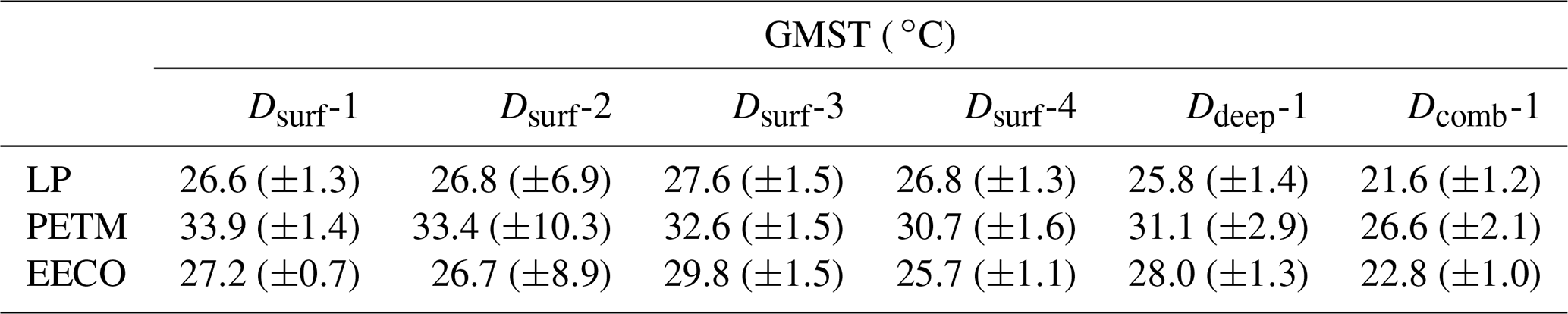
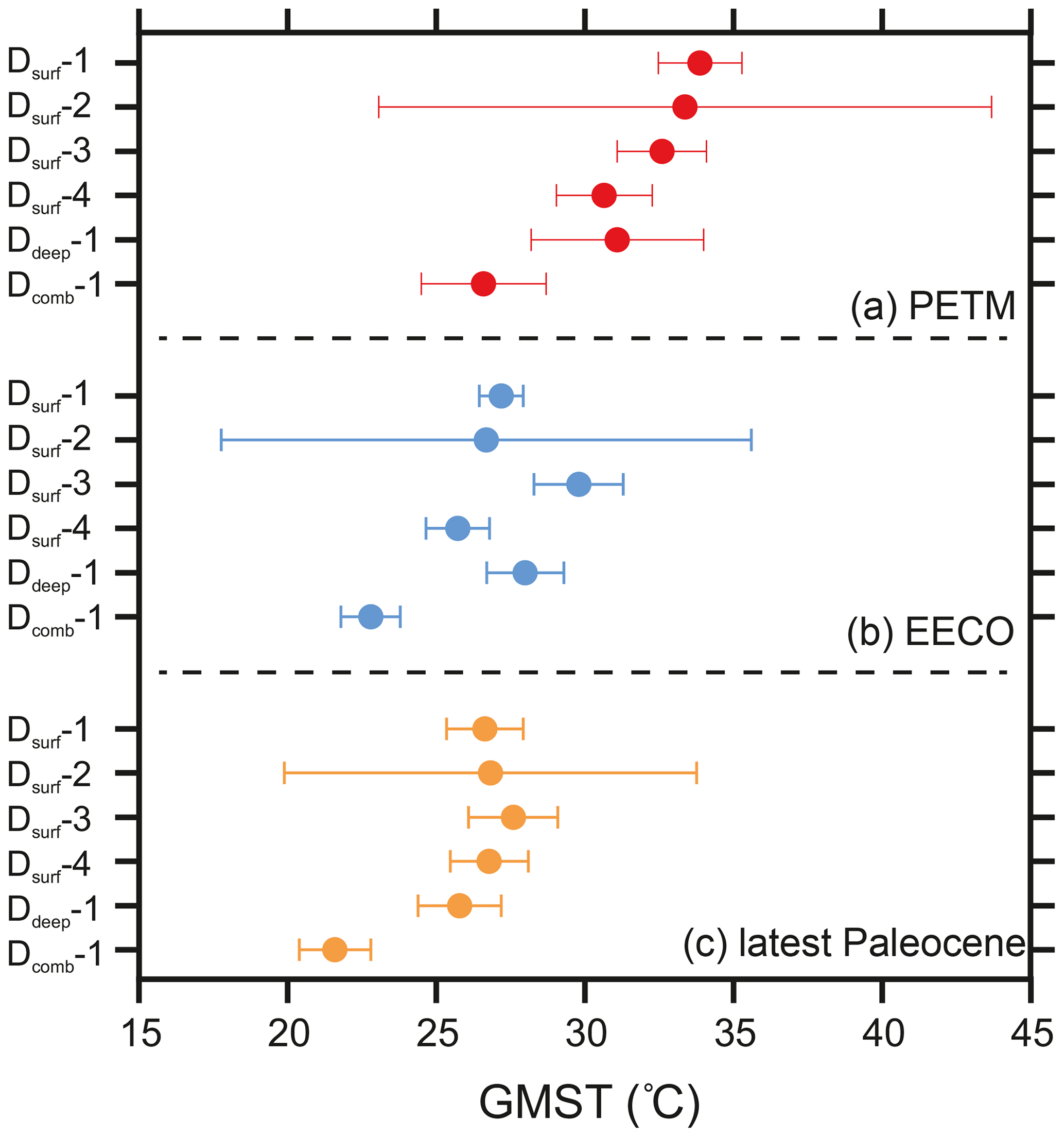
Figure 6 GMST estimates during the (a) PETM, (b) EECO, and (c) latest Paleocene for each methodology. GMST estimates utilise baseline experiments except D_surf-1 during the EECO, which uses D_surf-NoPaleosol. GMST estimates are based on the mantle-based reference frame. Error bars on each individual method are the standard deviation (1σ), except D_surf-1 and D_surf-2, which use the standard error (1σ_x).

GMST estimates for the latest Paleocene, PETM, and EECO, calculated using D_deep, are 25.8 ^∘C (±1.4 ^∘C), 31.1 (±2.9 ^∘C), and 28.0 ^∘C (±1.3 ^∘C), respectively (Table 3; Fig. 6). These estimates are comparable to those derived from surface temperature proxies alone (Table 3). GMST estimates from the EECO are also comparable to previous estimates based on globally distributed benthic foraminifera data (∼28 ^∘C; Hansen et al., 2013). As benthic foraminifera are less susceptible to diagenetic alteration than planktonic foraminifera (e.g. Edgar et al., 2013), this implies that benthic foraminiferal δ¹⁸O values could be used to provide the “fine temporal structure” of Cenozoic temperature change (e.g. Lunt et al., 2016; Hansen et al., 2013). However, we also urge caution as this approach scales GMST directly to BWT prior to the Pliocene and assumes that the characteristics of polar amplification are constant through time (see Evans et al., 2018; Cramwinckel et al., 2018). Changes in ice volume may also influence the benthic foraminiferal δ¹⁸O signal (see Hansen et al., 2013), and additional corrections are required before applying this method to other time intervals (e.g. the Eocene–Oligocene transition). D_deep also implies that vertical ocean stratification is fixed, even though vertical ocean stratification has been proposed to change dramatically in the past (e.g. Sijp et al., 2013; Goldner et al., 2014) and may shift the slope and/or intercept of the relationship between BWT and GMST.

GMST estimates for the latest Paleocene, PETM, and EECO, calculated using D_comb, are 21.6 ^∘C (±1.2 ^∘C), 26.6 (±2.1 ^∘C), and 22.8 ^∘C (±1.0 ^∘C), respectively (Fig. 6). These estimates are consistently lower (up to 5 ^∘C) than GMST estimates derived using D_surf and D_deep. Although D_comb-1 can estimate modern GMST within ∼1 to 2  ^∘C of measured values, whether this approach can be applied in greenhouse climates remains to be confirmed. As described above, we used CESM1 simulations (EO3 and EO4 from Cramwinckel et al., 2018) to compare the “true” model simulation GMST to that calculated using D_comb-1 (Supplement). We find that D_comb-1 underestimates GMST by 1 ^∘C during the Eocene when the model high-latitude SST is used as a proxy for the deep ocean and 2–3 ^∘C when the model deep-ocean temperature is used. As such, we suggest that D_comb-1 may reflect a minimum GMST constraint. We suggest that variable weighting of the deep ocean and tropics could improve the D_comb method in future studies (Eq. 5 gives an equal weighting to each).

3.2 Influence of different proxy datasets upon D_surf-derived GMST estimates

To explore the importance of the proxies themselves for D_surf-derived GMST estimates, we conducted a series of illustrative subsampling experiments relative to D_surf-baseline (Table 2). This was performed for methods D_surf-1, D_surf-2, D_surf-3, and D_surf-4. In the first subsampling experiment (D_surf-Frosty; Table 2), we include δ¹⁸O SST estimates from recrystallised planktonic foraminifera. This yields lower GMST estimates (<1 to 4 ^∘C; e.g. Figs. S6–S8) and is consistent amongst all four methods. This agrees with previous studies which indicate that δ¹⁸O values from recrystallised planktonic foraminifera are significantly colder than estimates derived from the δ¹⁸O value of well-preserved foraminifera (Pearson et al., 2001; Sexton et al., 2006; Edgar et al., 2015), foraminiferal Mg∕Ca ratios (Creech et al., 2010; Hollis et al., 2012), and clumped isotope values from larger benthic foraminifera (Evans et al., 2018).

The removal of TEX₈₆ results in lower GMST estimates (∼1 to 4 ^∘C; e.g. Figs. S6–S8) across all methodologies (D_surf-NoTEX; Table 2). This is consistent with previous studies which indicate that TEX₈₆ gives slightly higher SSTs than other proxies, especially in the middle to high latitudes (e.g. Hollis et al., 2012; Inglis et al., 2015). The functional response of TEX₈₆ at higher-than-modern SSTs remains relatively uncertain, which may explain why TEX₈₆ gives slightly higher SSTs than other proxies (see discussion in Hollis et al., 2019). New indices or calibrations could help to reduce the uncertainty associated with TEX₈₆-derived SST estimates beyond the modern calibration range. TEX₈₆ values can also be complicated by the input of isoGDGTs from other sources (see discussion in Hollis et al., 2019). The DeepMIP database excludes samples with anomalous GDGT distributions (Hollis et al., 2019). However, a Gaussian process regression (GPR) model may help to better identify anomalous GDGT distributions in the sedimentary record using a nearest-neighbour distance metric (Eley et al., 2019). This methodology could be employed in future studies to further refine GDGT-based SST datasets, but this methodology is currently under review and is not considered here. Despite the caveats and concerns raised in previous work, the exclusion of TEX₈₆ data shifts GMST by a relatively small amount.

The input of brGDGTs from archives other than mineral soils or peat can bias LAT estimates towards lower values (Inglis et al., 2017; Hollis et al., 2019), and the exclusion of MBT(') ∕ CBT-derived LAT estimates could yield higher GMST values. Excluding MBT(') ∕ CBT in marine sediments does yield slightly warmer GMST estimates (0.5 to 1.0 ^∘C). However, the impact of excluding MBT(') ∕ CBT values is relatively minor because there are other proxies (e.g. pollen assemblages, leaf floral) which yield comparable LAT estimates in the regions where MBT(') ∕ CBT values are removed (e.g. the SW Pacific).

The removal of δ¹⁸O values from paleosols and mammals as well as paleosol climofunctions (D_surf-NoPaleosol; Table 2) also leads to slightly warmer GMST estimates (∼0.5 ^∘C). This may be related to additional controls on paleosol and mammal δ¹⁸O values. This includes variations in the isotopic composition of rainfall (i.e. meteoric δ¹⁸O; Hyland and Sheldon, 2013), variations in soil water δ¹⁸O values (Hyland and Sheldon, 2013), and/or δ¹⁸O heterogeneity within nodules (e.g. Dworkin et al., 2005). Temperature estimates from paleosol climofunctions may also be prone to underestimation (e.g. Sheldon, 2009), and Hyland and Sheldon (2013) suggest that paleosol climofunctions are only applied as an indicator of relative temperature change. Intriguingly, the D_surf-1 method yields much higher GMST estimates during the EECO when δ¹⁸O values from paleosols and mammals as well as paleosol climofunctions are excluded (∼3 ^∘C higher than D_surf-baseline). This is attributed to the inclusion of two “cold” LAT estimates from the Salta Basin, NW Argentina (Hyland et al., 2017), which overly influence GMST (e.g. Fig. 2). For D_surf-1, a direct comparison of new and prior estimates (Caballero and Huber, 2013) can be made in which the only change has been the use of a newer data compilation. For our new estimate, the EECO is ∼4.5 ^∘C colder than previous estimates (29.75 ^∘C; Caballero and Huber, 2013). Given that the floristic LAT estimates are identical between the DeepMIP compilation and the older compilation, the lower GMST estimates are largely due to the incorporation of additional LAT datasets (e.g. paleosol climofunctions).

3.3 A combined estimate of GMST during the DeepMIP target intervals

To derive a combined estimate of GMST during the latest Paleocene, PETM, and EECO, we employ a probabilistic approach, using Monte Carlo resampling with full propagation of errors. Our combined estimate employs GMST estimates from each baseline experiment (except D_surf-1 for the EECO for which we use D_surf-NoPaleosol; see discussion above). We generated 1 000 000 iterations for each of the six methods for each time interval (latest Paleocene, PETM, and EECO). In these iterations, the GMST estimates were randomly sampled with replacement within their full uncertainty envelopes, assuming a Gaussian distribution of errors. As the different GMST estimates ultimately derive from the same proxy dataset, we do not consider them to be independent. The resulting 6 000 000 GMST iterations for each time period are thus simply added into a single probability density function in order to fully represent uncertainty (Fig. 7). This is equivalent to a linear pooling approach with equal weights (Genest and Zidek, 1986). From this probability distribution, the median value and the upper and lower limits corresponding to 66 % and 90 % confidence limits were identified (Table 4).

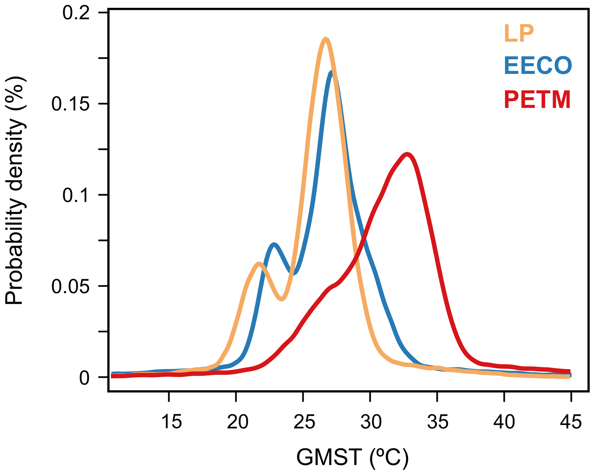
Figure 7 Probability density function of combined GMST during the DeepMIP intervals with full propagation of errors. GMST estimates are calculated on the mantle-based reference frame.

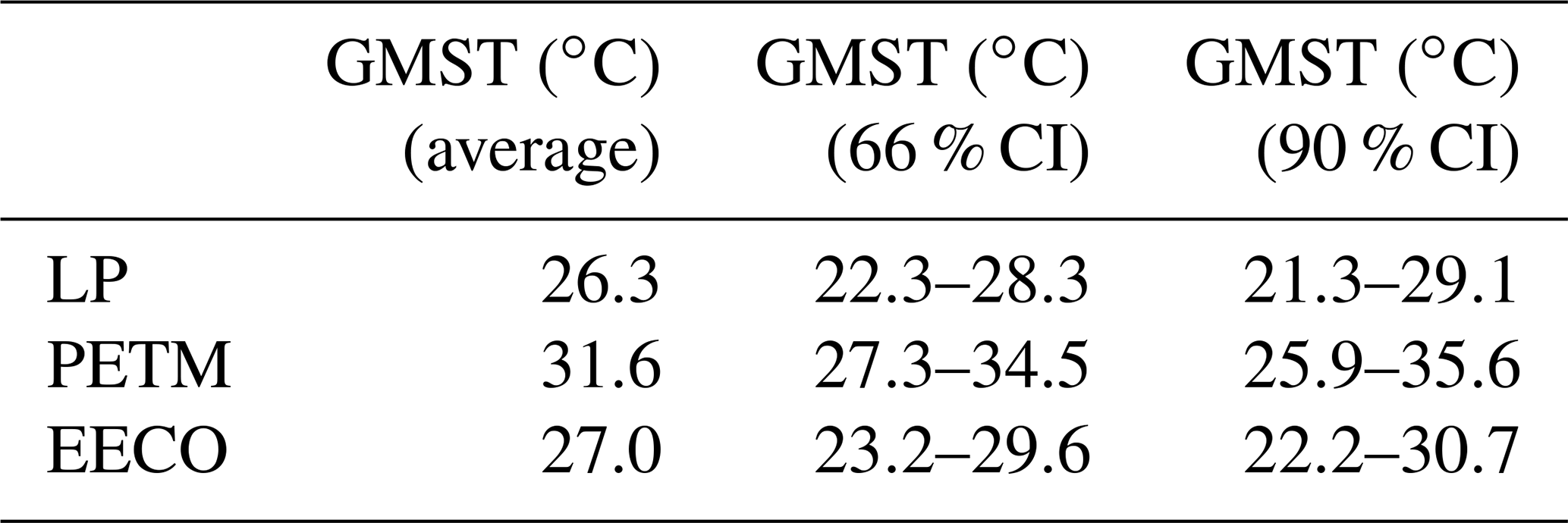
Table 4 Combined GMST estimates (66 % and 90 % confidence intervals) during the (i) latest Paleocene (LP), (ii) PETM, and (iii) EECO.

Sequential removal of one GMST method at a time (jackknife resampling) was performed to examine the influence of a single method upon the average GMST estimate. Jackknifing reveals that no single method overly influences the mean GMST or 66 % confidence intervals during the latest Paleocene, PETM, or EECO (±1.5 ^∘C; Supplement and Fig. S9). However, the removal of D_surf-2 (which has relatively large error bars; Fig. 6) reduces the 90 % confidence interval (Supplement). We also show that removing D_comb-1 removes the bimodality of the temperature distribution (Fig. S9). This is because D_comb-1 is associated with consistently lower GMST estimates compared to other methods (see Sect. 3.1).

During the latest Paleocene, the average GMST estimate is 26.3 ^∘C and ranges between 22.3 and 28.3 ^∘C (66 % confidence interval; Table 4; Fig. 7). During the PETM, the average GMST is higher (31.6 ^∘C) and ranges between 27.2 and 34.5 ^∘C (66 % confidence interval; Table 4; Fig. 7). Assuming a pre-industrial GMST of 14 ^∘C, our average GMST estimates indicate that the latest Paleocene and PETM are 12.3 and 17.6 ^∘C warmer than pre-industrial, respectively. Our results indicate that GMST likely increased by ∼4 to 6 ^∘C between the latest Paleocene and PETM (66 % confidence), in keeping with previous estimates (Frieling et al., 2019; Dunkley Jones, 2013). During the EECO, the average GMST estimate is 27.0 ^∘C and likely ranges between 23.2 and 29.7 ^∘C (66 % confidence interval; Table 4; Fig. 7). Assuming a pre-industrial GMST of 14 ^∘C, our average GMST estimate indicates that the EECO is 13.0 ^∘C warmer than pre-industrial. The GMST anomaly for the EECO is ∼2 ^∘C lower than previous studies (∼15 ^∘C warmer than pre-industrial; Caballero and Huber, 2013; Zhu et al., 2019), but the median falls within the range quoted previously in the IPCC AR5 (9 to 14 ^∘C warmer than pre-industrial). The EECO is approximately 4 to 5 ^∘C colder than the PETM (66 % confidence). This is larger than previously suggested (∼3 ^∘C; Zhu et al., 2019) and may be related to a cold bias in EECO GMST estimates (see Sect. 3.1).

3.4 Equilibrium climate sensitivity during the latest Paleocene, PETM, and EECO

Equilibrium climate sensitivity (ECS) can be defined as the equilibrium change in global near-surface air temperature resulting from a doubling in atmospheric CO₂. Various “flavours” of ECS exist, some of which specifically exclude various feedback processes not always included in climate models, such as those associated with ice sheets, vegetation, or aerosols (Rohling et al., 2012). ECS may also be state-dependent (Caballero and Huber, 2013), and there is no reason to expect that it has not changed with time or as a function of climate state (Farnsworth et al., 2019; Zhu et al., 2020). Therefore, direct comparison of ECS in the past to modern conditions is a fraught enterprise. For our purposes we define a bulk ECS (ECS_bulk) as being a gross estimate of ECS between our three intervals and pre-industrial, i.e.

$$\begin{array}{}\text{(6)}& {\mathrm{ECS}}_{\mathrm{bulk}}=\left(\mathrm{\Delta }{T}_{\mathrm{CO}\mathrm{2}-\mathrm{vs}-\mathrm{PI}}\right)/\left(\mathrm{\Delta }{F}_{\mathrm{CO}\mathrm{2}-\mathrm{vs}-\mathrm{PI}}\right),\end{array}$$

where $\mathrm{\Delta }{T}_{\mathrm{CO}\mathrm{2}-\mathrm{vs}-\mathrm{PI}}$ is the temperature difference between pre-industrial and the time period of interest that can be attributed to CO₂ forcing, and $\mathrm{\Delta }{F}_{\mathrm{CO}\mathrm{2}-\mathrm{vs}-\mathrm{PI}}$ is the CO₂ forcing relative to pre-industrial. The result is then normalised to a CO₂ forcing equal to a doubling of CO₂. Such calculations have been performed previously (e.g. Anagnostou et al., 2016) and they provide some constraint on the range of climate sensitivity values that are relevant for near-modern prediction (Rohling et al., 2012). For example, Anagnostou et al. (2016) indicated that early Eocene ECS (excluding ice sheet feedbacks) falls within the range 2.1–4.6 ^∘C per CO₂ doubling, with maximum probability for the EECO of 3.8 ^∘C. These values (2.1–4.6 ^∘C per CO₂ doubling) are similar to the IPCC ECS range (1.5–4.5 ^∘C at 66 % confidence). Here we calculate bulk ECS estimates using the change in GMST and CO₂ in the latest Paleocene, PETM, and EECO intervals with reference to the pre-industrial. Following the approach of Anagnostou et al. (2016) and using the forcing equation of Byrne and Goldblatt (2014), we first determine the relative change in climate forcing relative to pre-industrial ($\mathrm{\Delta }{F}_{\mathrm{CO}\mathrm{2}-\mathrm{vs}-\mathrm{PI}})$:

$$\begin{array}{}\text{(7)}& \mathrm{\Delta }{F}_{\mathrm{CO}\mathrm{2}-\mathrm{vs}-\mathrm{PI}}=\mathrm{5.32}\ln (C_t/C_{\mathrm{PI}})+\mathrm{0.39}\left[\ln \right(C_t/C_{\mathrm{PI}}){]}^{\mathrm{2}},\end{array}$$

where C_PI is the atmospheric CO₂ concentration during pre-industrial (278 ppm) and C_t refers to the CO₂ reconstruction at a particular time in the Eocene. The mean proxy estimate of CO₂ for the PETM is ∼2200 ppmv ($+\mathrm{1904}/-\mathrm{699}$ ppmv; 95 % confidence) (Gutjahr et al., 2017). The mean proxy estimate of CO₂ for the LP is ∼870 ppmv (Gutjahr et al., 2017). The uncertainty of latest Paleocene CO₂ represents 2 standard deviations of pre-PETM CO₂ (Gutjahr et al., 2017), equal to ±400 ppm. The mean proxy estimate of CO₂ for the EECO is ∼1625 ppmv (±750 ppmv; 95 % confidence) (Anagnostou et al., 2016; Hollis et al., 2019). To calculate bulk ECS, we then use radiative forcing from a doubling of CO₂ from Byrne and Goldblatt (2014) to translate CO₂ into forcing relative to pre-industrial (ΔF_CO2):

$$\begin{array}{}\text{(8)}& \mathrm{ECS}=\left(\mathrm{\Delta }{T}_{\mathrm{CO}\mathrm{2}-\mathrm{vs}-\mathrm{PI}}\right)/\mathrm{\Delta }{F}_{\mathrm{CO}\mathrm{2}-\mathrm{vs}-\mathrm{PI}}\times \mathrm{3.875},\end{array}$$

where GMST (ΔT) distributions are based on output generated via our Monte Carlo simulations (see Sect. 3.3). Some of the temperature anomaly of the latest Paleocene, PETM, and EECO is caused not by CO₂ but by the different paleotopography, paleobathymetry, and solar constant compared with pre-industrial. Furthermore, we choose here to calculate an ECS that explicitly excludes feedbacks associated with vegetation, ice sheets, and aerosols, i.e. $S_{[\mathrm{CO}\mathrm{2},\mathrm{LI},\mathrm{VG},\mathrm{AE}]}$ in the nomenclature of Rohling et al. (2012). To account for these effects, we subtract a value of 4.5 ^∘C (Caballero and Huber, 2013; Zhu et al. 2019) from GMST; i.e.

$$\begin{array}{}\text{(9)}& \mathrm{\Delta }{T}_{\mathrm{CO}\mathrm{2}-\mathrm{vs}-\mathrm{PI}}=\mathrm{\Delta }\mathrm{GMST}-\mathrm{4.5}{}^{\circ }\mathrm{C}.\end{array}$$

Following Anagnostou et al. (2016), the uncertainty of the slow-feedback correction on ΔGMST follows a uniform “flat” probability (±1.5 ^∘C). This value of 4.5 ^∘C is based upon a comparison of pre-industrial and Eocene simulations (both 1×CO₂) conducted with CESM1.2 (Zhu et al., 2019), which incorporates the paleogeographic, solar constant, ice sheet, vegetation, aerosol, and ice sheet changes from pre-industrial to Eocene. Our value is similar to previous studies which attribute ∼4 to 6 ^∘C to non-CO₂ and non-aerosol forcings and feedbacks (Anagnostou et al., 2016; Caballero and Huber, 2013, Lunt et al., 2012). However, the sensitivity to these Eocene boundary conditions is likely model-dependent and this value may differ between model simulations. The uncertainties in our estimated ECS are the products of 10 000 realisations of the latest Paleocene, PETM, and EECO CO₂ values as well as the respective ΔGMST estimate (the mean estimate and propagated uncertainty) based on randomly sampling each variable within its 66 % and 90 % confidence interval uncertainty envelope.

Table 5 Estimates of ECS (66 % and 90 % confidence) during the (i) latest Paleocene (LP), (ii) PETM, and (iii) EECO.

$S_{[\mathrm{CO}\mathrm{2},\mathrm{LI},\mathrm{VG},\mathrm{AE}]}$ values (66% confidence) for the EECO and PETM average 0.80 (0.46 to 1.15) and 0.92 (0.60 to 1.20), respectively. This yields ECS estimates (66 % confidence) for the EECO and PETM compared to modern which average 3.1 ^∘C (1.8 to 4.4 ^∘C) and 3.6 ^∘C (2.3 to 4.7 ^∘C), respectively (Table 5; Fig. 8). These are broadly comparable to previous estimates from the early Eocene which account for paleogeography and other feedbacks (∼2.1 to 4.6 ^∘C; Anagnostou et al., 2016). They are also similar to those predicted by the IPCC (1.5 to 4.5 ^∘C per doubling CO₂). $S_{[\mathrm{CO}\mathrm{2},\mathrm{LI},\mathrm{VG},\mathrm{AE}]}$ values (66 % confidence) during the latest Paleocene average 1.16 (0.61 to 1.75), which is somewhat higher than the other DeepMIP intervals. This yields ECS estimates (66 % confidence) for the latest Paleocene which average 4.5 ^∘C (2.4 to 6.8 ^∘C) (Table 5; Fig. 8). Higher ECS values are attributed to relatively high GMST estimates (∼26 ^∘C) and relatively low CO₂ values (∼870 ppm) during the latest Paleocene. As latest Paleocene CO₂ estimates remain highly uncertain (Gutjahr et al., 2017; see above), new high-fidelity CO₂ records are required to accurately constrain ECS during this time.

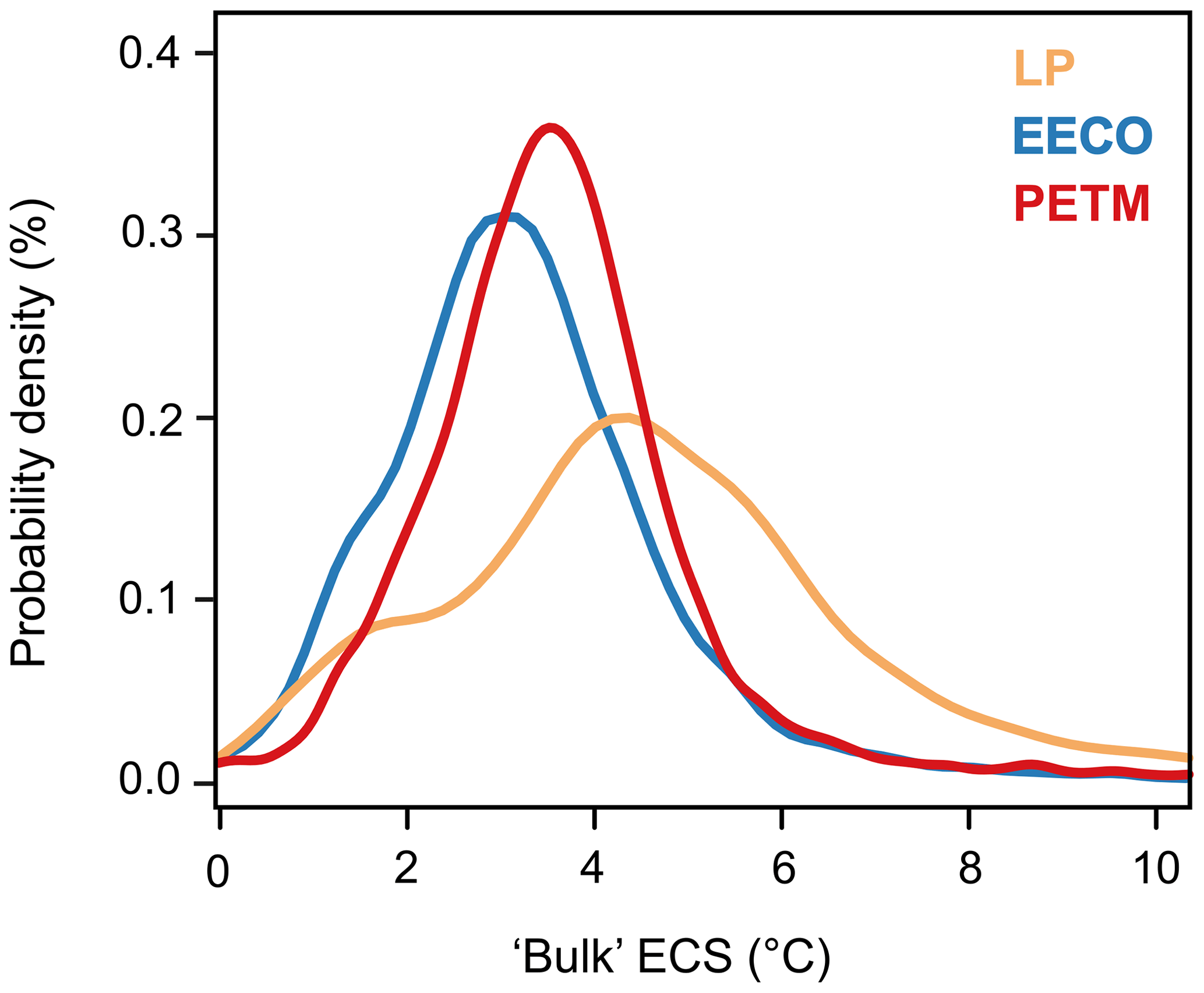
Figure 8 Probability density function of bulk ECS during the latest Paleocene, PETM, and EECO that explicitly accounts for non-CO₂ forcings of paleogeography and the solar constant, as well as feedbacks associated with land ice, vegetation, and aerosols (Zhu et al., 2019), i.e. $S_{[\mathrm{CO}\mathrm{2},\mathrm{LI},\mathrm{VG},\mathrm{AE}]}$ in the nomenclature of Rohling et al. (2012).

ECS may be strongly state-dependent, and model simulations indicate a non-linear increase in ECS at higher temperatures (Caballero and Huber, 2013; Zhu et al., 2019) due to changes in cloud feedbacks (Abbot et al., 2009; Caballero and Huber, 2010; Arnold et al., 2012; Zhu et al., 2019). This implies caution when relating geological estimates to modern climate predictions (e.g. Rohling et al., 2012; Zhu et al., 2020) and it may be more appropriate to calculate ECS between different time intervals (e.g. latest Paleocene to PETM; Shaffer et al., 2016). To this end, we also calculate ECS between the transition from the latest Paleocene to the PETM, assuming that non-CO₂ forcings and feedbacks are negligible. This yields an ECS estimate of 3.6 ^∘C. However, early Paleogene CO₂ estimates remain uncertain (Gutjahr et al., 2017), and well-synchronised, continuous, and high-resolution CO₂ records are required to accurately constrain ECS during the DeepMIP intervals.

4 Conclusions

Using six different methods, we have quantified global mean surface temperatures (GMSTs) during the latest Paleocene, PETM, and EECO. GMST was calculated within a coordinated, experimental framework and utilised six methodologies including three different input datasets. After evaluating the impact of different proxy datasets upon GMST estimates, we combined all six methodologies to derive an average GMST value during the latest Paleocene, PETM, and EECO. We show that the “average” GMST estimate (66 % confidence) during the latest Paleocene, PETM, and EECO is 26.3 ^∘C (22.3 to 28.3 ^∘C), 31.6 ^∘C (27.2 to 34.5 ^∘C), and 27.0 ^∘C (23.2 to 29.7 ^∘C), respectively. Assuming a pre-industrial GMST of 14 ^∘C, the latest Paleocene, PETM, and EECO are 12.3 ^∘C, 17.6, and 13.0 ^∘C warmer than modern, respectively. Using our “combined” GMST estimate, we demonstrate that “bulk” ECS (66 % confidence) during the latest Paleocene, PETM, and EECO is 4.5 ^∘C (2.4 to 6.8 ^∘C), 3.6 ^∘C (2.3 to 4.7 ^∘C), and 3.1 ^∘C (1.8 to 4.4 ^∘C) per doubling of CO₂. Taken together, this study improves our characterisation of the global mean temperature of these key time intervals, allowing future climate change to be put into the context of past changes and allowing us to provide a refined estimate of ECS.