Sensitivity of mid-Pliocene climate to changes in orbital forcing and PlioMIP's boundary conditions

We compare results obtained from modeling the mid-Pliocene warm period using the Community Earth System Models (COSMOS, version: COSMOS-landveg r2413, 2009) with the two different modeling methodologies and sets of boundary conditions prescribed for the two phases of the Pliocene Model Intercomparison Project (PlioMIP), tagged PlioMIP1 and PlioMIP2. Here, we bridge the gap between our contributions to PlioMIP1 (Stepanek and Lohmann, 2012) and PlioMIP2 (Stepanek et al., 2020). We highlight some of the effects that differences in the chosen mid-Pliocene model setup (PlioMIP2 vs. PlioMIP1) have on the climate state as derived with COSMOS, as this information will be valuable in the framework of the model–model and model–data comparison within PlioMIP2. We evaluate the model sensitivity to improved mid-Pliocene boundary conditions using PlioMIP's core mid-Pliocene experiments for PlioMIP1 and PlioMIP2 and present further simulations in which we test model sensitivity to variations in paleogeography, orbit, and the concentration of CO₂.

Firstly, we highlight major changes in boundary conditions from PlioMIP1 to PlioMIP2 and also the challenges recorded from the initial effort. The results derived from our simulations show that COSMOS simulates a mid-Pliocene climate state that is 0.29 ^∘C colder in PlioMIP2 if compared to PlioMIP1 (17.82 ^∘C in PlioMIP1, 17.53 ^∘C in PlioMIP2; values based on simulated surface skin temperature). On the one hand, high-latitude warming, which is supported by proxy evidence of the mid-Pliocene, is underestimated in simulations of both PlioMIP1 and PlioMIP2. On the other hand, spatial variations in surface air temperature (SAT), sea surface temperature (SST), and the distribution of sea ice suggest improvement of simulated SAT and SST in PlioMIP2 if employing the updated paleogeography. Our PlioMIP2 mid-Pliocene simulation produces warmer SSTs in the Arctic and North Atlantic Ocean than those derived from the respective PlioMIP1 climate state. The difference in prescribed CO₂ accounts for 0.5 ^∘C of temperature difference in the Arctic, leading to an ice-free summer in the PlioMIP1 simulation, and a quasi ice-free summer in PlioMIP2. Beyond the official set of PlioMIP2 simulations, we present further simulations and analyses that sample the phase space of potential alternative orbital forcings that have acted during the Pliocene and may have impacted geological records. Employing orbital forcing, which differs from that proposed for PlioMIP2 (i.e., corresponding to pre-industrial conditions) but falls into the mid-Pliocene time period targeted in PlioMIP, leads to pronounced annual and seasonal temperature variations. Our result identifies the changes in mid-Pliocene paleogeography from PRISM3 to PRISM4 as the major driver of the mid-Pliocene warmth within PlioMIP and not the minor differences in forcings.

1 Introduction

In 2050, the global population is expected to have increased by 2.7 billion relative to its 2005 value (Bongaarts, 2009). In conjunction with this population increase, energy demand is also rising. While short-term perspectives for a carbon-neutral global economy and effective CO₂ drawdown technologies are absent, a direct implication of population dynamics for the climate system is an increased concentration of atmospheric CO₂ through anthropogenic activities, increased waste heat from energy production that hampers the local climate of some parts of the world, loss of polar sea ice, and, last but not the least, rising global temperature. Through the continuous release of trace gases that impact the Earth's energy balance, such as CO₂, into the atmosphere and as a result of the vast thermal inertia of the Earth system, future warming is inevitable. In expectation of a warmer climate, it is of utmost importance to quantify climatic conditions that humankind could face in the near future in order to enable proper preparation and information about the need for and possibility of mitigation measures wherever possible. The mid-Pliocene warm period (mPWP) (3.264–3.025 million years (Ma) before present (BP); Dowsett et al., 2016) has been suggested as a time slice which could provide possible insight into future climate in terms of temperature (Jansen et al., 2007). Climate model simulations of this time slice suggest global mean temperatures 2–3 ^∘C higher than today (Haywood and Valdes, 2004; Jansen et al., 2007) with land surface conditions, continental configuration, and atmospheric concentrations of CO₂ that were similar, although not identical, to the present day (Raymo et al., 1996; Pagani et al., 2010; Kürschner et al., 1996; Haywood et al., 2016). Evidence from the geologic record suggests that in the past the Arctic was more vegetated than today, e.g., during the mid-Pliocene warm period (Rybczynski et al., 2013). These records of the past offer us a glimpse into a climate of increased temperatures in polar regions that may return in the next decades (Overland et al., 2014) as an effect of the human influence on climate. Hence, the mid-Pliocene can be considered a useful, but not direct, analog for future warmth (Jansen et al., 2007).

Characteristics of mid-Pliocene climate can be inferred either through records of past climate that were stored in geological archives or by exposing climate models to boundary conditions and model forcing representative of the Earth system characteristics of the period. These may include altered continental configuration, past land elevation and ocean bathymetry, and the atmospheric composition and orbital configuration representative of the period under study. Furthermore, a parameterization of altered vegetation distribution may be necessary if it is not dynamically computed by the model itself. Creating boundary conditions for past time periods is one of the most time-consuming tasks faced in paleoclimate modeling. Assumptions with respect to the implementation of details of paleoclimate boundary conditions can vary amongst researchers, and the mid-Pliocene is not an exceptional time slice in this respect. To provide common grounds for the model intercomparison in simulating the mPWP and to reduce the need for repeating simulations with updated model setups, the Pliocene Modelling Intercomparison Project (PlioMIP) provides for phases 1 (PlioMIP1; Haywood et al., 2010, 2011) and 2 (PlioMIP2; Haywood et al., 2016) sets of boundary conditions that are implemented consistently across the model ensemble.

As shown in the framework of PlioMIP1 (e.g., Haywood et al., 2013a), PlioMIP provides a unique opportunity to reconcile our knowledge about the mechanisms in, and the characteristics of, a warmer climate. In this framework, consistency of various climate model simulations of the mPWP, and their ability to reproduce climate patterns that have been inferred from data stored in geological climate archives, is sampled and compared in a coordinated effort. To support this ambition in PlioMIP2, we provide in this paper important information that relates Community Earth System Models (COSMOS) simulations, contributed to both PlioMIP1 (Stepanek and Lohmann, 2012) and PlioMIP2 (Stepanek et al., 2020), to each other. In this effort we study how differences in the boundary conditions and model forcing, which are present between COSMOS simulations for PlioMIP1 and PlioMIP2 as a result of updates to the relevant PlioMIP/PMIP protocols, influence various large-scale climate patterns. To provide boundary conditions for the climate models and to derive model-independent paleoclimate information that can be employed for a model–data comparison, PlioMIP works in alliance with the US Geological Survey's Pliocene Research Interpretation and Synoptic Mapping (PRISM) project that has constantly improved the data basis for the Pliocene paleoenvironment over the last 25 years (e.g., Dowsett et al., 2013). All boundary conditions presented in this paper are directly based on output from the PRISM project. Following the conclusion of PlioMIP1, PlioMIP2 utilizes state-of-the-art boundary conditions that have emerged over the last few years, with updated reconstructions of ocean bathymetry and land ice, surface topography, and new datasets describing the distribution of mid-Pliocene soils and lakes (Haywood et al., 2016). With the exception of the lake reconstruction, all these datasets are employed in our PlioMIP2 simulations (Stepanek et al., 2020). Lakes cannot be adequately represented in the employed model setup of COSMOS (Stepanek et al., 2020). While this reduces comparability between COSMOS and other models in PlioMIP2 that employ the full set of boundary conditions provided in the enhanced dataset (Haywood et al., 2016), it improves comparability between COSMOS simulations of PlioMIP2 and PlioMIP1; in the latter lakes are also not considered. Here, we specifically address improved paleogeography and the change in mPWP concentrations of atmospheric CO₂ from PlioMIP1 to PlioMIP2. Furthermore, we take the opportunity to go beyond the PlioMIP2 protocol (Haywood et al., 2016) and sample the impact of alternative orbital forcing, which could have shaped the reconstructed climate over the time period from 3.26 to 3.025 Ma BP, on our modeled climate state. Our aim is to test the extent to which alternative configurations of the Earth's orbit during the mPWP could potentially improve the agreement of modeled and reconstructed mPWP climate states. For this, we compared two climate states within the mPWP representative of Marine Isotope Stages (MISs) KM5c and K1. KM5c has been selected for simulations within PlioMIP2 due to its strong similarity to modern day in terms of orbital forcing (Haywood et al., 2016). MIS K1, on the other hand, refers to an interval which witnessed about 0.5 Wm⁻² more annual insolation than modern day (Prescott et al., 2014).

2 Methodology

2.1 Evolution of mid-Pliocene model paleogeography and forcing

Paleogeographic boundary conditions for simulating the Pliocene have undergone major changes from PlioMIP1 to PlioMIP2. The switch from PRISM3D (Dowsett et al., 2010) to PRISM4 (Dowsett et al., 2016) has led to the introduction of various changes in the mPWP model setup of COSMOS. Updates to topography and bathymetry reflect changes in dynamic topography, global isostatic adjustment, and new findings that suggest a reduced extent of the Greenland Ice Sheet (Haywood et al., 2016; Dowsett et al., 2016). The PRISM4 Antarctic ice sheet, on the other hand, remains over East Antarctica, consistent with the version suggested by PRISM3D (Haywood et al., 2016, and references therein) (compare Fig. 1a and b).

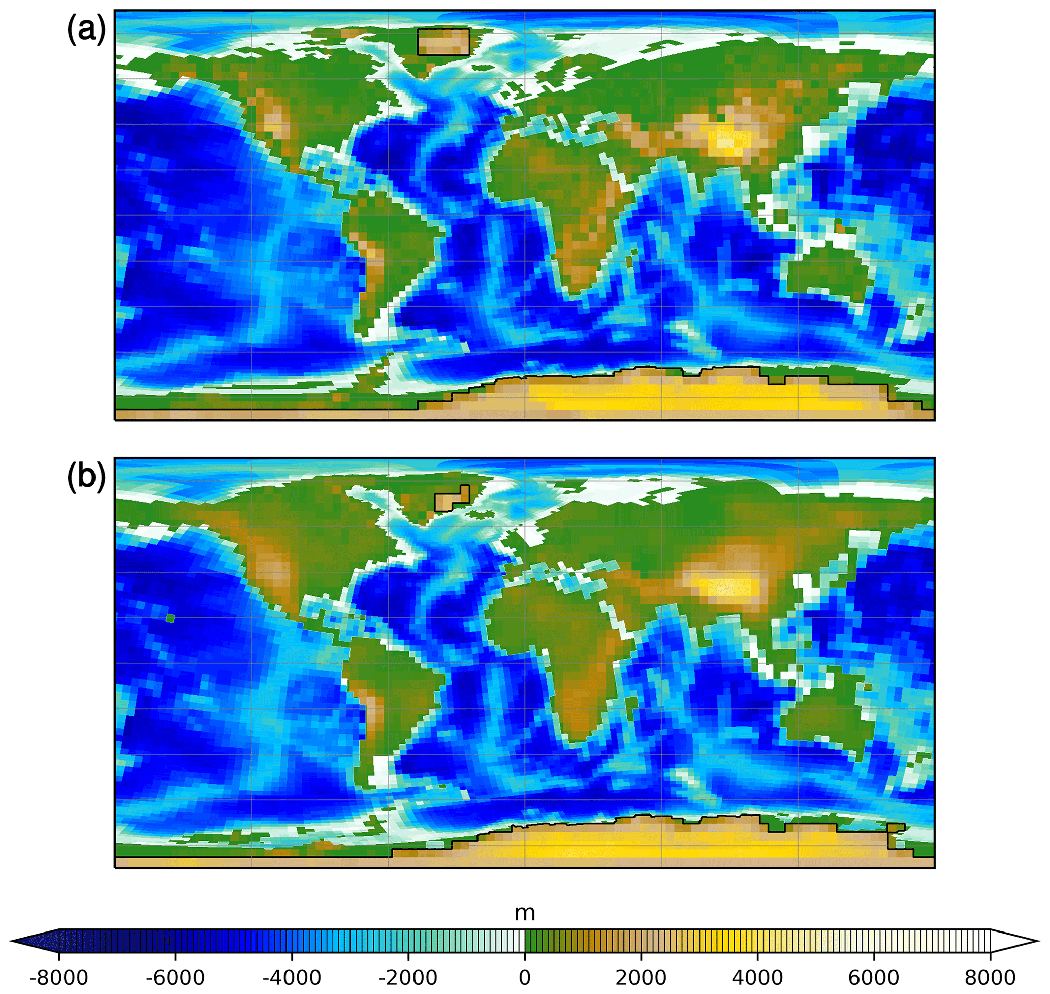
Figure 1 (a) PRISM3D land–sea mask implemented in COSMOS simulations for PlioMIP1 based on data provided by Haywood et al. (2010), assuming the presence of an open Bering Strait and Canadian Arctic Archipelago. (b) PRISM4 land–sea mask implemented in COSMOS simulations for PlioMIP2 with a closed Bering Strait and Canadian Arctic Archipelago as described in the PlioMIP2 protocol (Haywood et al., 2016; Dowsett et al., 2016). Color shading depicts the prescribed land orography and ocean bathymetry (m) for PlioMIP1 and PlioMIP2, respectively. Black isolines depict prescribed mid-Pliocene ice sheets for the respective phases of PlioMIP. Differences over Antarctica are due to the switch from employing a modern land–sea mask with minor modifications towards Pliocene conditions in the COSMOS PlioMIP1 simulation and employing a full Pliocene representation of Antarctic geography in COSMOS for PlioMIP2.

A major difference between the PlioMIP2 and PlioMIP1 model setup is the configuration of two ocean gateways – the Bering Strait, which is closed in PlioMIP2 by separating the Bering Sea and Chukchi Sea with a land bridge, and the Canadian Arctic Archipelago; both were open in PlioMIP1 (compare Fig. 1a and b). Based on previous work, closing these gateways increases modeled sea surface temperature (SST) in the North Atlantic Ocean, which would reduce the apparent disagreement of models and reconstructions in this region (Dowsett et al., 2013; Otto-Bliesner et al., 2016). Closing the Bering Strait is supported by evidence that this gateway may have been temporarily closed in proximity to the mPWP (Matthiessen et al., 2008).

A high concentration of atmospheric CO₂ is often presented as one of the major reasons for the relatively higher than present-day temperatures during the mid-Pliocene (Seki et al., 2010; Pagani et al., 2010). However, the exact concentration of atmospheric CO₂ during this time slice remains uncertain, with various values being suggested (Raymo et al., 1996; Kürschner et al., 1996; Haywood et al., 2010, 2011, 2016), which complicates a comparison between models and reconstructions. Within PlioMIP, the absence of reconstructions for other radiative–active trace gases is acknowledged, and the respective radiative forcing is absorbed into an increased value of CO₂ – yet, this value differs between PlioMIP1 and PlioMIP2 (Haywood et al., 2010, 2016). Furthermore, between PlioMIP1 and PlioMIP2 the concentrations of the pre-industrial (PI) control state of COSMOS changed due to an update of the reference setup to the PMIP4 protocol (Otto-Bliesner et al., 2017), implying small differences in the employed concentrations of methane and nitrous oxide in COSMOS between PlioMIP2 and PlioMIP1. While these changes are small, we do not want to neglect their potential effect on climatic differences between PlioMIP2 and PlioMIP1 COSMOS simulations. Therefore, here we study the effect of differences between the trace gas forcing of both iterations of PlioMIP on the climate of the mPWP as simulated with COSMOS.

One additional topic addressed in this study is the potential for varying orbital forcing that may have influenced the mPWP over time. Both PlioMIP1 and PlioMIP2 assume a modern orbit for simulations of the mPWP (Haywood et al., 2010, 2011, 2016). This choice represents only one of multiple orbits that were present during the PlioMIP period, spanning Marine Isotope Stage (MIS) G21 to M1 (Haywood et al., 2016). Prescribing present-day orbital forcing that is very close to the configuration during the KM5c time slice selected for PlioMIP2 (Haywood et al., 2016) may not reproduce the expected warm or cold condition that could have been enabled by an orbit that occurred sometime during the mPWP. This is a side effect of computing an average mPWP condition rather than attempting to study the transient climate evolution of the mPWP within PlioMIP – such a study would be a promising approach to identify orbitally forced warm peaks but is beyond the capabilities of the model intercomparison. Most of the mismatches recorded between mid-Pliocene model simulations and interpretations of data stored in geological archives have been attributed to the choice of orbital forcing prescribed for model simulations (Haywood et al., 2013b; Prescott et al., 2014). The need for a more discrete time slice for simulating the mPWP towards an improved model–data comparison has been stated (Haywood et al., 2013a). Thus, the KM5c time slice has been selected, partly on the basis of the strong similarity of the orbit at that time to the modern orbital configuration. This is useful towards interpreting paleoenvironments in the context of future warming (Haywood et al., 2016) based on anthropogenic activity and will obviously be set in a nearly modern orbital configuration. While acknowledging the utility of the KM5c orbit for the scientific aims of PlioMIP2, here we go beyond the simulation of KM5c and quantify the effect of an alternative orbital configuration. We create model setups in which the prescribed PlioMIP2 model setup for COSMOS employs an orbital configuration that is representative of MIS K1. The MIS K1 time slice is one of the lightest isotope excursions found during the mPWP, with the total global annual mean insolation being approximately 0.5 W m⁻² higher than modern (Prescott et al., 2014). The effect of orbital forcing on the mPWP has been studied by Prescott et al. (2014), with an emphasis on surface air temperature (SAT). The novelty in our approach is that we employ the updated PlioMIP2 model setup and also test the impact of orbital configuration on the ocean state, in particular on SST and sea ice. Furthermore, we put differences in orbital forcing into context with varying concentrations of CO₂.

2.2 Model description COSMOS

The coupled atmosphere–ocean model used to produce simulations for this study is COSMOS, which was developed by the Max Planck Institute for Meteorology (MPI) in Hamburg, Germany. COSMOS consists of four major components, namely the ECHAM5 atmosphere model (Roeckner et al., 2003), the MPI-OM ocean model (Marsland et al., 2003), the land–vegetation and carbon cycle model JSBACH (Raddatz et al., 2007), and the ocean biogeochemistry model HAMOCC. The latter was introduced by Maier-Reimer (1993) but is not used in the production of PlioMIP simulations. For a description of the coupled setup and an evaluation of its performance, please refer to Jungclaus et al. (2006). COSMOS has already proven to be a valuable tool for the study of paleoclimate, also beyond the Pliocene epoch. The various time slices studied by means of COSMOS include, but are not limited to, the last millennium (Jungclaus et al., 2010), warm climates of the Miocene (e.g., Knorr et al., 2011), the mid-Pliocene (Stepanek and Lohmann, 2012), and glacial (e.g., Gong et al., 2013; Kageyema et al., 2013; X. Zhang et al., 2013) and interglacial climates (e.g., Pfeiffer and Lohmann, 2016; Varma et al., 2012; Wei and Lohmann, 2012). A detailed description of the COSMOS model components is given by Stepanek and Lohmann (2012).

2.3 Experimental designs

The aim of this study is to identify and discuss differences in the modeled climate that occur between the COSMOS simulations contributed to PlioMIP1 and PlioMIP2 and to study the effect of orbits warmer than the configuration applied for PlioMIP. With this aim in mind, we have applied a methodology for setting up simulations as described below. In general, experiments were carried out following PlioMIP1 and PlioMIP2 protocols (Haywood et al., 2010, 2011, 2016). Yet, for the purpose of this study, small modifications to the proposed official PlioMIP model setups are necessary. Three different orbits are employed here (Table 1). Two of them are similar and representative of modern and PI conditions – the only difference between them is small deviations that were introduced into the reference setup of COSMOS between PlioMIP1 and PlioMIP2 via adaptation of the PI orbit in COSMOS according to the PMIP4 protocol (Otto-Bliesner et al., 2017). The third employed configuration represents the orbit of MIS K1, with the values of orbital parameters being based on the astronomical solution by Laskar et al. (2004). Earth's orbital parameters are prescribed as constant values of eccentricity, obliquity, and the longitude of perihelion as outlined in Table 1. The orbit employed for simulating K1 is consistent with the configuration chosen by Prescott et al. (2014).

Table 1 Detailed description of experiments including the category of orbital configuration based on two different pre-industrial (PI) and one mPWP-specific setting, as well as specific parameter values and applied geography.

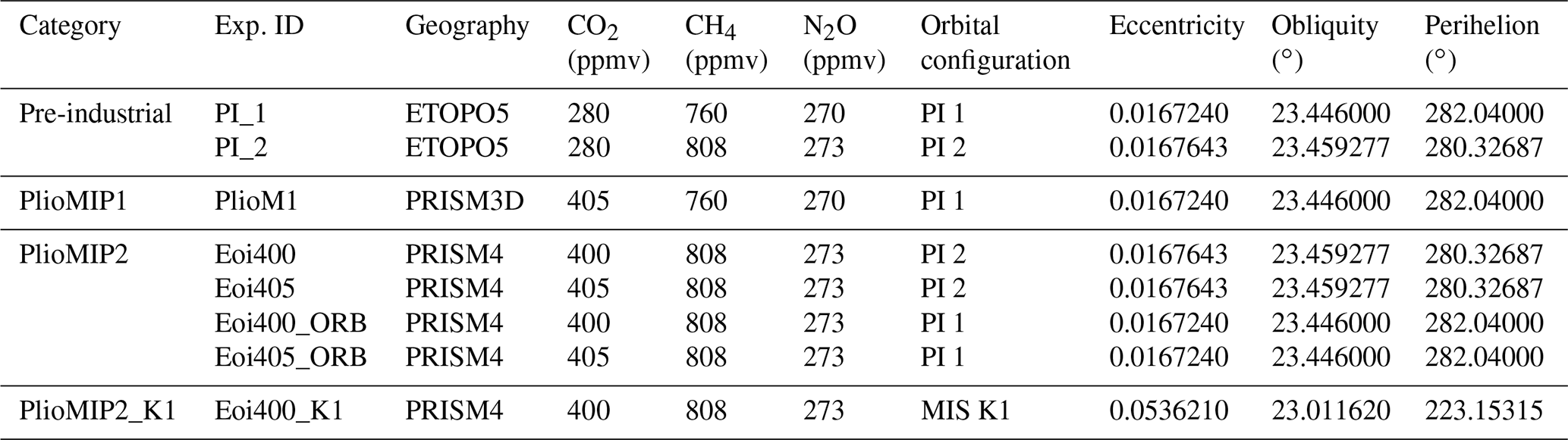
Simulations are classified into four different categories, namely PI, standard PlioMIP1 setup, standard PlioMIP2 setup, and modified PlioMIP2 setup with adapted (MIS K1) orbit (PlioMIP2_K1). First in the order as shown in Table 1 is the PI category, which consists of the PI control simulations (PI_1 and PI_2) for PlioMIP1 and PlioMIP2, respectively. The ocean bathymetry and land–sea mask are taken from the standard modern setup of COSMOS. As described by Jungclaus et al. (2006), this setup has been generated based on the Earth Topography Five Minute Grid (ETOPO5; National Geophysical Data Center, 1988; Edwards, 1992). An identical CO₂ concentration of 280 ppmv is prescribed for PI_1 and PI_2, but both experiments differ slightly with respect to orbital parameters and the volume mixing ratios of trace gases N₂O and CH₄ (see Table 1). The constant volume mixing ratios of 270 ppbv of N₂O and 760 ppbv of CH₄ are prescribed for PI_1, while the corresponding values for PI_2 are set to 273 and 808 ppbv, respectively. Chlorofluorocarbons, on the other hand, are absent across all simulations. Category PlioMIP1 consists of simulation PlioM1, which is the coupled ocean–atmosphere COSMOS mid-Pliocene experiment within the framework of PlioMIP1 (Stepanek and Lohmann, 2012) and utilizes the PRISM3D land–sea mask, orography, and ice mask. Category PlioMIP2 consists of mid-Pliocene simulations based on PRISM4 boundary conditions with slight differences in either orbital forcing or the concentration of atmospheric CO₂. Simulation Eoi400 is the COSMOS mid-Pliocene experiment for PlioMIP2 (Stepanek et al., 2020) in which CO₂ is prescribed to be 400 ppmv, while simulation Eoi405 is derived from Eoi400 in that the concentration of carbon dioxide is set to the PlioMIP1 CO₂ forcing of 405 ppmv. In comparing them, both simulations enable us to study the impact of the difference in CO₂ forcing between the two phases of PlioMIP on achieved results. Furthermore, simulation Eoi400_ORB employs the orbital forcing utilized by COSMOS in simulating the mid-Pliocene for PlioMIP1, while retaining other boundary conditions and forcing as prescribed for PlioMIP2. Direct comparison between simulations Eoi400 and Eoi400_ORB will give an indication of the influence of the slight change in orbital forcing on mid-Pliocene climate as simulated with COSMOS for PlioMIP1 and PlioMIP2. This is important within the framework of PlioMIP, for which orbital forcing is described as similar to modern day, but specific PI orbital parameters differ in the case of COSMOS between PlioMIP1 and PlioMIP2. Simulation Eoi405_ORB of category PlioMIP2 differs from simulation PlioM1 (Stepanek and Lohmann, 2012) in that it employs the paleoenvironmental reconstruction of PRISM4 and also employs different trace house gas concentrations for methane and nitrous oxide. It differs from simulation Eoi400, on the other hand, in both orbital configuration and the prescribed concentration of carbon dioxide (see Table 1). This choice of modeling methodology enables us to infer the relative effects of the improved representation of mid-Pliocene geography from PlioMIP1 to PlioMIP2 on our model, while honoring the presence of other differences in the model setup. Furthermore, in order to study the effect of an alternative orbit on mid-Pliocene warmth, simulation Eoi400_K1 in category PlioMIP2_K1 is consistent with the standard mid-Pliocene setup prescribed for PlioMIP2 and employed in simulation Eoi400, but it employs a different orbital forcing which is representative of MIS K1. The choice of our experimental design, enabling a direct comparison between simulations Eoi400 and Eoi400_K1, provides an indication of orbitally influenced climatic variability within the mid-Pliocene. Ultimately, the total effect of all the improved boundary conditions in PlioMIP2 is examined by comparing simulations PlioM1 and Eoi400. All simulations are integrated for 1500 years and are well equilibrated before being analyzed. Figure S1, added as the Supplement to this paper, shows time series of the Atlantic Meridional Overturning Circulation index to illustrate the equilibration, integration length, and time period (green shading) with which analyses are carried out for all simulations.

3 Results

This section present results of the mid-Pliocene and PI simulations listed in Table 1 and attempts to investigate and quantify the differences in the mid-Pliocene climate simulations by COSMOS for PlioMIP1 and PlioMIP2. Furthermore, we present results from our sensitivity experiments, which show the relative contributions of newly prescribed PlioMIP2 boundary conditions (Haywood et al., 2016) with respect to those of PlioMIP1 (Haywood et al., 2010, 2011) in the context of deviations of the COSMOS model setup between PlioMIP1 and PlioMIP2 that are not due to the PlioMIP2 protocol. We also show simulated seasonal variability, which may occur due to orbital forcing prescribed in simulating the mid-Pliocene climate. This is examined by a direct comparison of climate forced by two distinct orbital configurations representative of two discrete time slices within the mid-Pliocene, namely MIS K1 and the PlioMIP2 reference orbit MIS KM5c. MIS KM5c is selected for simulations within the framework of PlioMIP2 due to its strong orbital similarity to the present day (Haywood et al., 2016), and thus the present-day orbital configuration is adopted (Otto-Bliesner et al., 2017). Since the aim of this study is to infer the major driver of the mid-Pliocene warmth, we dedicate our analyses to SAT, SST, and sea ice distribution. Anomalies are tested with regard to significance in the context of internal variability in the contributing simulations by means of the autocorrelation method by Matalas and Dawdy (1964). Furthermore, a comparison between simulated precipitation for PlioM1 and Eoi400 (Fig. S3 in the Supplement) largely shows no appreciable difference spatially and when averaged across latitude.

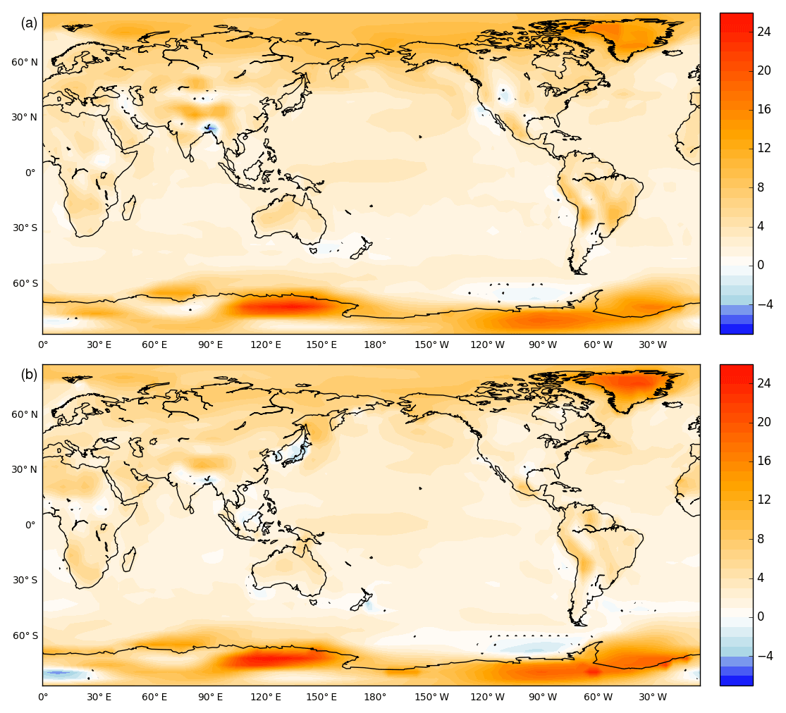
Figure 2 Annual mean SAT (^∘C) anomalies between core mid-Pliocene simulations for PlioMIP1 and PlioMIP2, with their respective pre-industrial simulations (PI_1 and PI_2). (a) Climatological anomaly that has been calculated over 100 years for PlioMIP1; panel (b) is as panel (a), but for Eoi400. Stipples (black dots) show regions of statistically insignificant differences.

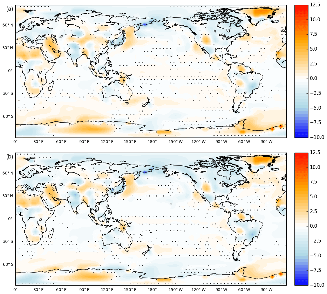
Figure 3 Annual mean SAT (^∘C) anomalies between mid-Pliocene simulations with varying boundary conditions. (a) Eoi405_ORB − PlioM1, which shows the contribution of changes in mid-Pliocene paleogeography between PlioMIP1 and PlioMIP2. (b) Comparison (Eoi400 − PlioM1) of mid-Pliocene simulations of both PlioMIP phases, incorporating all the changes from PlioMIP1 to PlioMIP2.

3.1 Comparison of selected climatic variables between PlioMIP1 and PlioMIP2

At large scale, COSMOS simulates fairly similar patterns of mid-Pliocene SAT in response to boundary conditions for PlioMIP1 and PlioMIP2 core experiments. Yet, there are noteworthy differences in the details of mid-Pliocene SAT anomalies between PlioMIP2 and PlioMIP1. The most pronounced annual average SAT anomaly of mPWP relative to PI occurs in both phases of PlioMIP at high latitudes and in polar regions, providing evidence of a similar, albeit not identical, level of polar amplification in the PlioMIP1 and PlioMIP2 mPWP model setups. On average, COSMOS simulates a mid-Pliocene climate that is 0.29 ^∘C colder in PlioMIP2, with the global average SAT reaching 290.97 ^∘C for PlioMIP1, while the corresponding value for PlioMIP2 is 290.68 ^∘C. It is important to note that the aforementioned values are recomputed based on averaging over 100 years, while Stepanek and Lohmann (2012) have, in agreement with the PlioMIP1 analysis protocol, provided averages over 30 years. PlioM1 and Eoi400 show that SAT anomalies are fairly similar over the equatorial oceans but that there is substantial deviation of SAT over continents and polar regions (Figs. 2a, b and 3b). The most pronounced relative warming is seen over Greenland and Antarctica. On the other hand, gradual cooling is present over the Arctic from PlioM1 to Eoi400. Over the oceans, COSMOS simulates warmer SAT over the North Atlantic for Eoi400, while SAT over the Indian Ocean, South Atlantic Ocean, and low-latitude Pacific Ocean is largely unchanged. Generally, both PlioM1 and Eoi400 simulations suggest that landmasses are warmer than the ocean and furthermore that there is substantial polar amplification; the latter is more pronounced in PlioM1 (compare Figs. 2a, b and 3b). The strong regional warming simulated over Greenland and Antarctica is linked to changes in albedo and orography over these regions from PlioMIP1 to PlioMIP2 (compare Fig. 1a and b). The magnitude of changes in albedo and elevation over Greenland are more pronounced in Eoi400 than in PlioM1 (Fig. 1a and b) due to a reduction in the spatial extent of the Greenland Ice Sheet from PRISM3D to PRISM4 (Dowsett et al., 2016). Consequently, the regional warming signal is also more pronounced in PlioMIP2 (Fig. 3b). For PlioM1, a warming of about 15 ^∘C is found over Greenland, while the corresponding value is about 21 ^∘C for Eoi400. This illustrates that the mPWP SAT anomaly simulated with COSMOS is regionally increased in Eoi400 relative to PlioM1, even though the global average mPWP temperature anomaly is smaller in Eoi400. Antarctic ice sheet estimates based on results produced with the British Antarctic Survey Ice Sheet Model utilizing a climate simulation produced with PRISM boundary conditions (Haywood et al., 2010) remain the same for both phases of PlioMIP (Dowsett et al., 2016; Haywood et al., 2016). Over Antarctica, there are strong regional mPWP temperature anomalies, while cooling is evident in the South Pacific between 60^∘ and 70^∘ S, extending from 65^∘ to 150^∘ W for both simulations. This South Pacific cooling is about −1.2 K on average in PlioMIP1 (PlioM1 with respect to PI_1) but more intense in PlioMIP2 (Eoi400 vs. PI_2), for which the temperature anomaly locally reaches −4 ^∘C and is characterized by a wider spatial extent. In both simulations (Eoi400 and PlioM1), the Indian sector of the Southern Ocean experiences intense warming that extends from 60^∘ E into the South Pacific Ocean. Extreme values of SAT anomalies vary from 25.2 ^∘C in PlioM1 to 23.1 ^∘C in Eoi400 over the adjacent Antarctic landmass. Moving the focus again to the Northern Hemisphere, we highlight the fact that both simulations PlioM1 and Eoi400 are characterized by land–sea masks in which the modern Hudson Bay is absent, while that region is part of the oceans in our PI simulation setups. The change in the land–sea mask introduces an annual mean warming in the mid-Pliocene in comparison to PI that is fairly similar in PlioM1 and Eoi400 but slightly stronger in PlioM1.

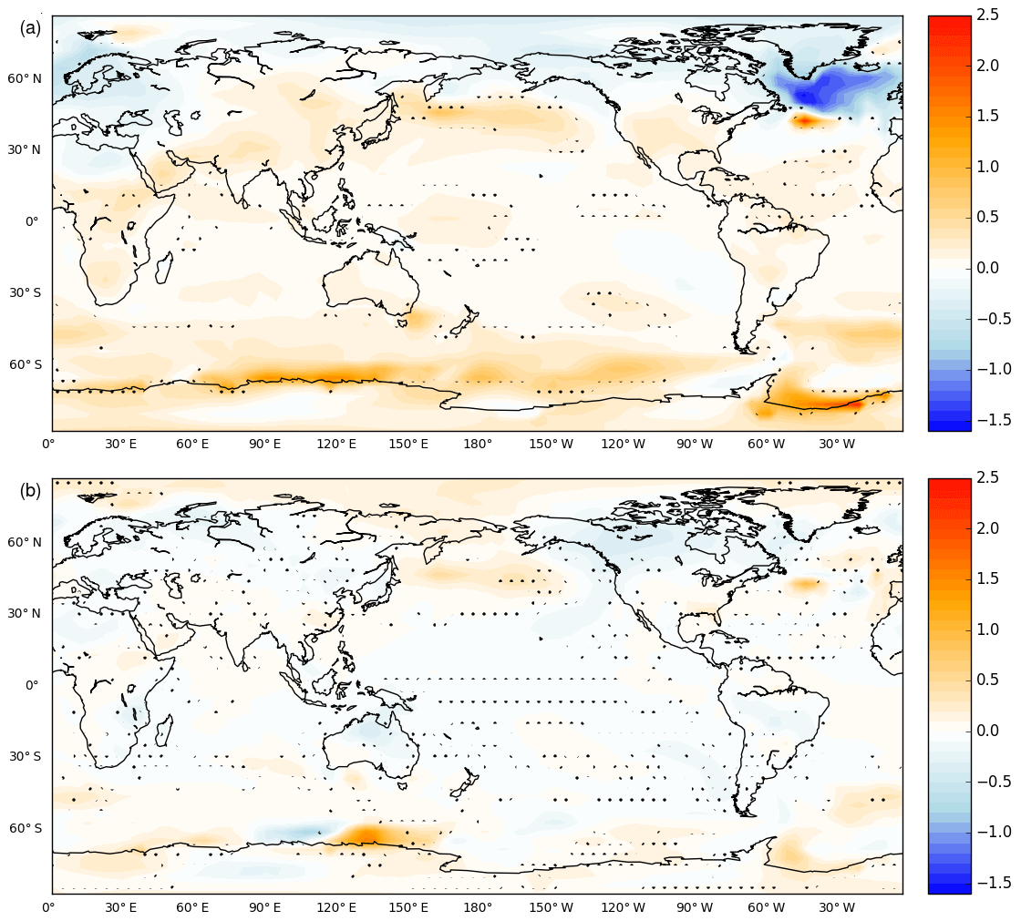
Figure 4 Annual mean SAT (^∘C) anomalies between mid-Pliocene simulations with varying boundary conditions. (a) Eoi405 − Eoi400, showing anomalies due to changes in mid-Pliocene CO₂ from 405 to 400 ppmv as utilized for PlioMIP1 and PlioMIP2, respectively, while (b) Eoi400_ORB − Eoi400 shows variations caused by changes in mid-Pliocene orbit utilized in COSMOS simulations for PlioMIP1 and PlioMIP2.

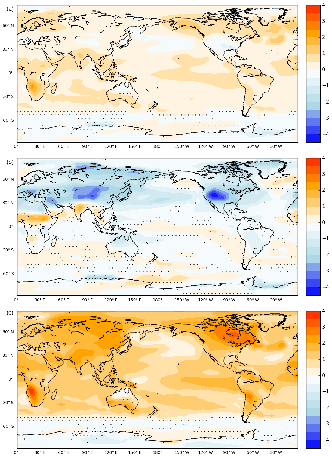
Figure 5 Annual and seasonal mean SAT anomalies due to a change in mid-Pliocene orbital forcing between Marine Isotope Stages K1 and KM5c, calculated from Eoi400_K1 − Eoi400. Shown are (a) annual mean SAT (^∘C), (b) boreal summer (JJA), and (c) boreal winter (DJF).

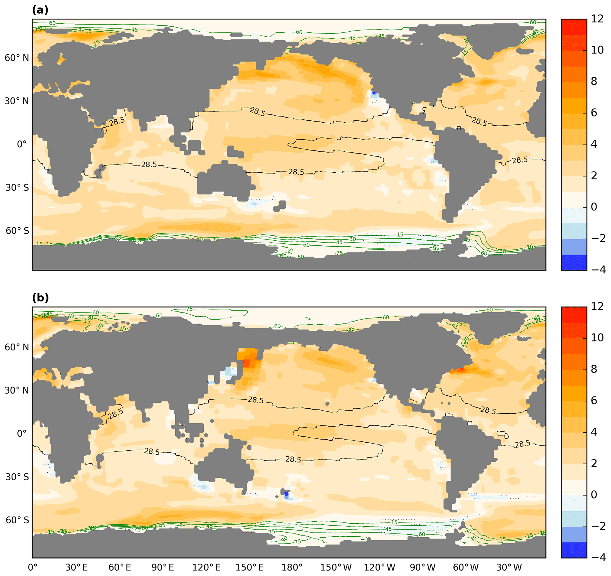
Figure 6 Comparison between mid-Pliocene SST (^∘C) anomalies calculated from 100 years of model output with respect to PI control simulations as obtained from COSMOS (a) PlioMIP1 and (b) PlioMIP2. Black isolines show the expansion of the equatorial warm pool in the mid-Pliocene state, while the green isolines depict absolute annual mean sea ice cover in the mid-Pliocene state. The contour interval for the sea ice isolines is 15 %.

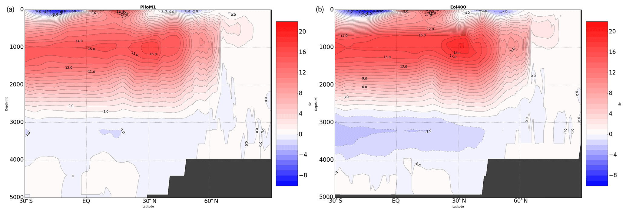
Figure 7 COSMOS-simulated mid-Pliocene annual mean AMOC in Sverdrups for (a) PlioMIP1 (simulation PlioM1) and (b) PlioMIP2 (simulation Eoi400). Overturning rates are time averages that have been calculated from 100-year model outputs. Positive values represent a clockwise circulation.

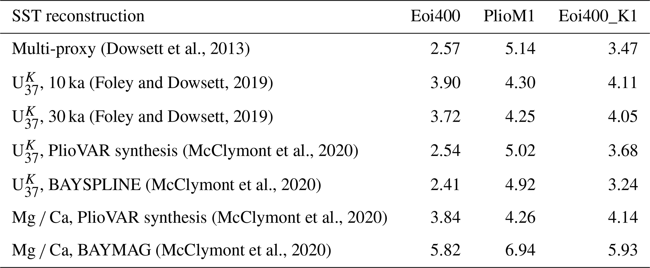
Analysis of sea surface temperature (SST) for both Eoi400 and PlioM1 shows the presence of the equatorial warm pool, which extends across all ocean basins of the world (Fig. 6). This warm pool is characterized as a pattern of warm water at the surface around the Equator and defined as the region where absolute SSTs exceed 28.5 ^∘C (Watanabe, 2008). In COSMOS simulations we find no change in the pattern of the equatorial warm pool between Eoi400 and PlioM1, as both realizations of the mid-Pliocene climate state show warm pools of an almost identical spatial extent (Fig. 6). Beyond the extent of the equatorial warm pool, we find similarity in SST anomalies obtained from the comparison of PlioM1 and Eoi400 to their respective PI control runs in many regions of the world. The Northern Hemisphere surface ocean is – with a few exceptions of regional cooling – characterized by regions of increased SST, a pattern that is more pronounced in the Pacific. Evidence from PlioMIP1 (Dowsett et al., 2013) suggests that mid-Pliocene North Atlantic SST, as derived from geological records, is consistently underestimated by the models. The COSMOS PlioMIP2 mid-Pliocene simulation produces a warmer North Atlantic than the respective PlioMIP1 simulation (compare Fig. 6a and b). As a result, the model–data discord in that region, which has been identified by Dowsett et al. (2013), is mitigated to some extent. This is confirmed by obtaining the root mean square deviation (RMSD) between COSMOS-simulated SSTs for both PlioM1 and Eoi400, as well as the SST reconstruction by Dowsett et al. (2013) taken from their Supplement Table S1. An RMSD of 5.14 is evident between reconstructed and modeled mid-Pliocene North Atlantic SSTs in PlioMIP1, while a corresponding RMSD of 2.57 is estimated in PlioMIP2 (Stepanek et al., 2020) (see Table 2). Better agreement between reconstructed and simulated North Atlantic SSTs for PlioMIP2 is linked to the strength of the Atlantic Meridional Overturning Circulation (AMOC) at different depths. Increased SSTs are accompanied by enhanced AMOC in the upper cell at about 1000 m of depth, which transports more heat to high latitudes of the Northern Hemisphere (Fig. 7a and b). Furthermore, the inflow of deep water from the South Atlantic, more precisely the transport of Antarctic Bottom Water, is stronger in Eoi400: AMOC at depths shallower than 3000 m is slightly enhanced from PlioMIP1 to PlioMIP2 (see Fig. 7a and b). Further comparisons between simulated SSTs and emerging reconstructions (McClymont et al., 2020; Foley and Dowsett 2019) show better agreement when compared with Eoi400 (Table 2). This highlights the fact that – independent of the proxy calibration, the chosen width of the time window of the reconstruction, or the proxy recorder type – the updated PlioMIP2 modeling protocol, including updated PRISM4 boundary conditions, improves the agreement between mid-Pliocene climate as simulated in COSMOS and as derived from the geologic record.

Table 2 Root mean square deviation between North Atlantic sea surface temperatures of selected mid-Pliocene simulations (Eoi400, PlioM1, and Eoi400_K1) and available reconstructions.

Annual mean sea ice is strongly reduced for both PlioMIP1 and PlioMIP2 mid-Pliocene simulations if compared to the respective PI simulation. The general pattern of mid-Pliocene sea ice is rather similar in that sea ice cover retreats towards the North Pole. For seasonal analysis of sea ice, the definition of seasons is different from the conventional December to February (boreal winter) and June to August (boreal summer) time period. In this study, with regard to sea ice, winter is rather defined as February to April (FMA) and summer rather as the months from August to October (ASO) (see Fig. 11). According to Howell et al. (2016), these are the 3-month periods in which more than half of the PlioMIP1 ensemble simulations show the highest and lowest mean sea ice extent, respectively. There are slight differences in prescribed orbital parameters for both PI simulations and the respective mid-Pliocene simulations considered in this study that employ an orbital forcing similar to that of PI. We find that differences in the orbital forcing have no effect on the large-scale seasonal pattern of PI Arctic sea ice, as our results show for respective simulations a similar spatial extent for both summer and winter (compare Fig. 11a and c, Fig. 11b and d). With the mPWP boundary conditions prescribed for PlioMIP1 and PlioMIP2, COSMOS simulates a considerably smaller sea ice extent for the mid-Pliocene with respect to PI simulations (compare Fig. 11e–h to Fig. 11a–d). The most obvious loss of sea ice in the mPWP is present around the Hudson Bay, which is represented as land for mid-Pliocene simulations. In contrast, our PI simulations show that the Hudson Bay is totally ice-free during summer, but the sea ice concentration at this location reaches a maximum during winter. The Canadian Arctic Archipelago is totally free of sea ice for mid-Pliocene simulations with PRISM4 geography. In addition to these trivial changes in sea ice, little or no sea ice is present around the Bering Strait during mid-Pliocene boreal summer. The combined effect of mid-Pliocene geography, orbit, and CO₂ (PlioM1 vs. Eoi400) shows that the mid-Pliocene Arctic Ocean is ice-free during summer. The sea ice concentration drops below 15 % in PlioM1, while for Eoi400 we find that summer sea ice is quasi-absent (compare Fig. 11f and h).

3.2 Contributions of paleogeography and changes in CO₂ to PlioMIP2

We suggest that changes in paleogeography between the two phases of PlioMIP may be the main contributor to the differences between mid-Pliocene SAT for PlioMIP1 and PlioMIP2, as simulated by COSMOS. Comparison between Eoi405_ORB and PlioM1, which accounts for the influence of the PRISM4 geography, interestingly shows a similar pattern as the total effect of all boundary conditions, the latter deduced from the difference between simulations Eoi400 and PlioM1 (compare Figs. 3a and b). The major difference between the effect of changed paleogeography and the total effect of all boundary conditions (including orbit) is noticed in the Arctic region, where cooling of a relatively higher magnitude is observed for the total effect. Furthermore, there are significant differences between these simulations, especially in regions where obvious changes in orography are applied.

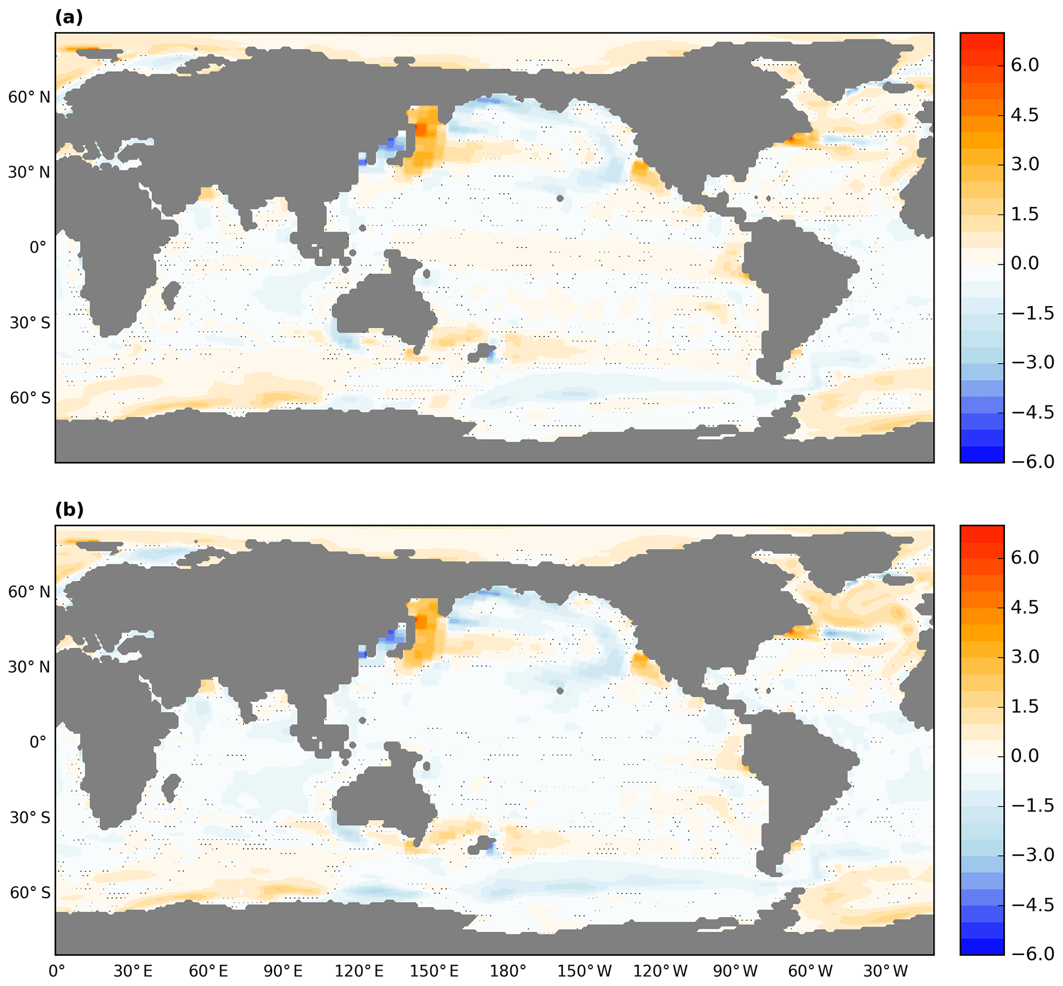
Figure 8 Annual mean SST (^∘C) anomalies between mid-Pliocene simulations with varying boundary and initial conditions. (a) Eoi405_ORB − PlioM1, which shows the contribution of changes in mid-Pliocene paleogeography between PlioMIP1 and PlioMIP2; (b) Eoi400 − PlioM1, comparing mid-Pliocene simulations of both phases of PlioMIP, incorporating all the changes in paleogeography, orbital, and greenhouse gas forcing from PlioMIP1 to PlioMIP2.

Similar to SAT, COSMOS simulates almost the same SST pattern in Eoi400 and PlioM1 when comparing the influence of PRISM4 geography to the total boundary condition effect (constituting geography, orbit, and atmospheric trace gases). Both mid-Pliocene simulations show the expected warming in the Arctic Ocean, North Atlantic Ocean, and also in the Indian and Atlantic sector of the Southern Ocean. In contrast to the total effect of PlioMIP2 boundary conditions, PRISM4 geography produces a warmer equatorial Pacific when implemented instead of PRISM3D geography together with other PlioMIP1 boundary and initial conditions (see Fig. 8a and b). This implies that the effect of geography on Arctic temperatures is different for atmosphere and ocean realms.

Figure 9 Annual mean SST (^∘C) anomalies between mid-Pliocene simulations with varying boundary conditions. (a) Eoi405 − Eoi400, quantifying anomalies due to changes in mid-Pliocene CO₂ from 405 to 400 ppmv, as utilized for PlioMIP1 and PlioMIP2, respectively. (b) Eoi400_ORB − Eoi400, quantifying changes in the (PI and KM5c) orbital configuration as utilized in COSMOS simulations for PlioMIP1 and PlioMIP2.

The relative contribution of CO₂ difference between PlioMIP1 and PlioMIP2 is investigated by comparing Eoi400 and Eoi405 (see Fig. 4 for SAT). The difference generally produces a warmer ocean surface in PlioMIP1 in comparison to the setup of PlioMIP2, which is more pronounced in the Southern Ocean (see Fig. 9a). When averaged over a 100-year period, the North Atlantic shows that a dipole of warm and cold ocean surface prevails as seen in SAT (see Fig. 4), with the maximum SST increase amounting to 2.9 ^∘C, while maximum cooling reaches −1.3 ^∘C as a result of increased CO₂. In contrast, when averaged over a longer time period (200 year), the magnitude of cooling in the region is largely reduced (Fig. S1). This cold blob is indeed not stable and is hence an artifact of internal variability in the model.

Finally, for sea ice, all simulations with PRISM4 geography produce sea ice with a larger spatial extent and concentration during summer months than is the case for their PRISM3D counterpart (PlioM1), irrespective of the specified concentration of atmospheric CO₂ (compare Fig. 12b, d, f, and h with Fig. 11f). Therefore, the change in CO₂ between PlioMIP1 and PlioMIP2 does not affect large-scale patterns of summer sea ice in the Arctic.

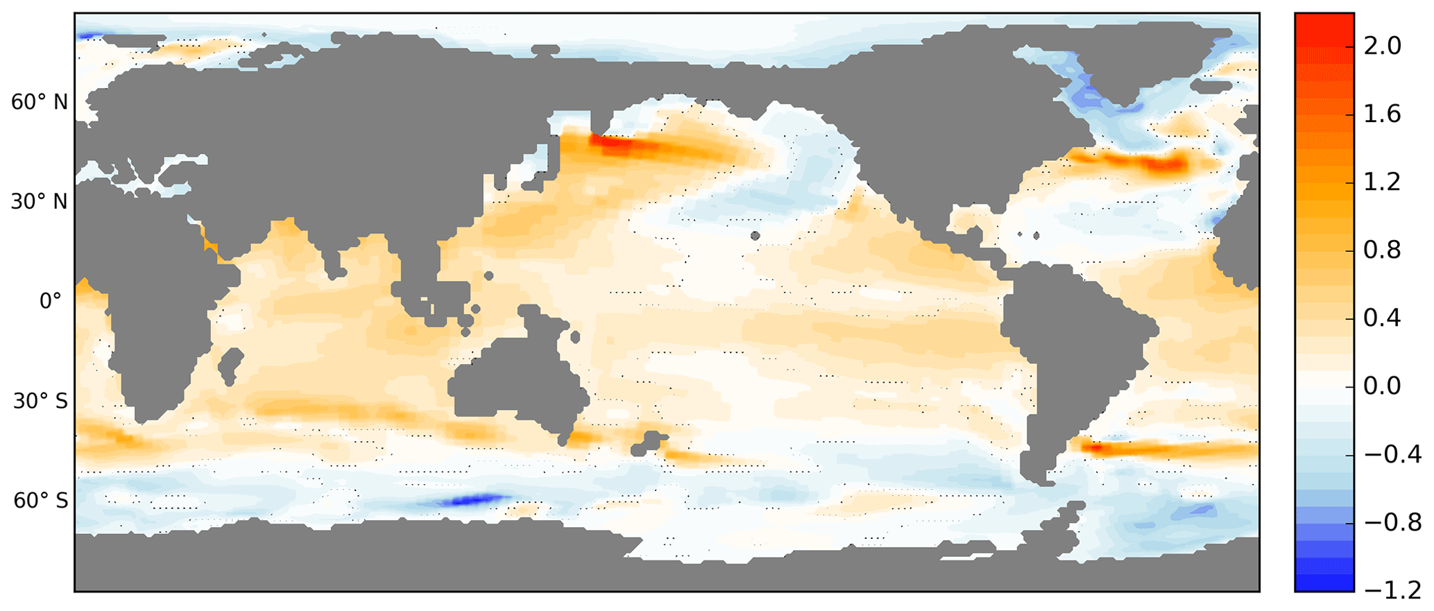
Figure 10 Annual mean SST anomalies due to a change in mid-Pliocene orbital forcing between Marine Isotope Stages K1 and KM5c, calculated from Eoi400_K1 − Eoi400.

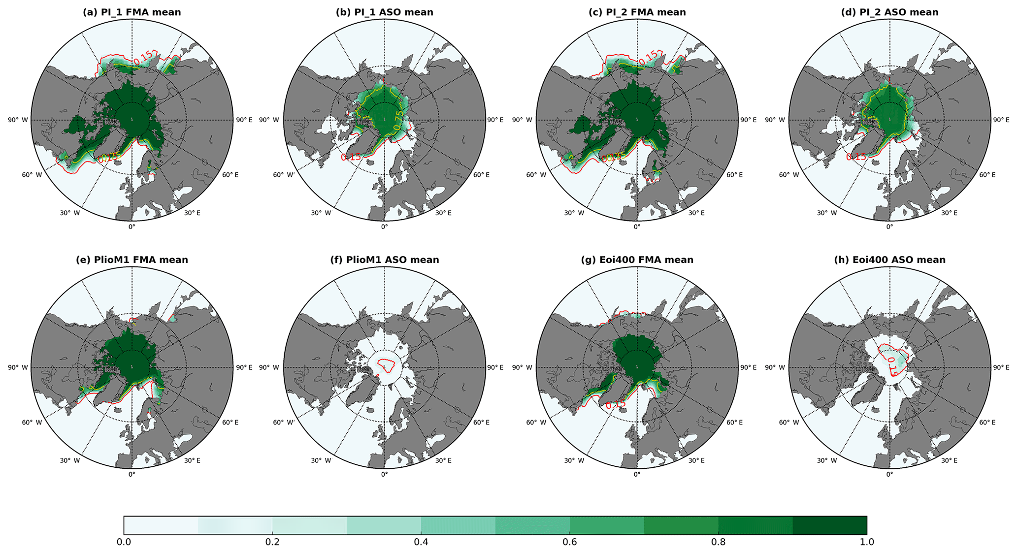
Figure 11 Seasonal mean Arctic sea ice concentration averaged over 100 model years as simulated by COSMOS for mid-Pliocene and PI runs in response to boundary conditions prescribed for PlioMIP1 and PlioMIP2. Panels (a), (c), (e), and (g) show winter (FMA) averages, while panels (b), (d), (f), and (h) show summer (ASO) averages for simulations PI_1, PI_2, PlioM1, and Eoi400, respectively. The red contours indicate the 15 % isoline of sea ice cover, while yellow contours indicate the 75 % isoline of sea ice cover.

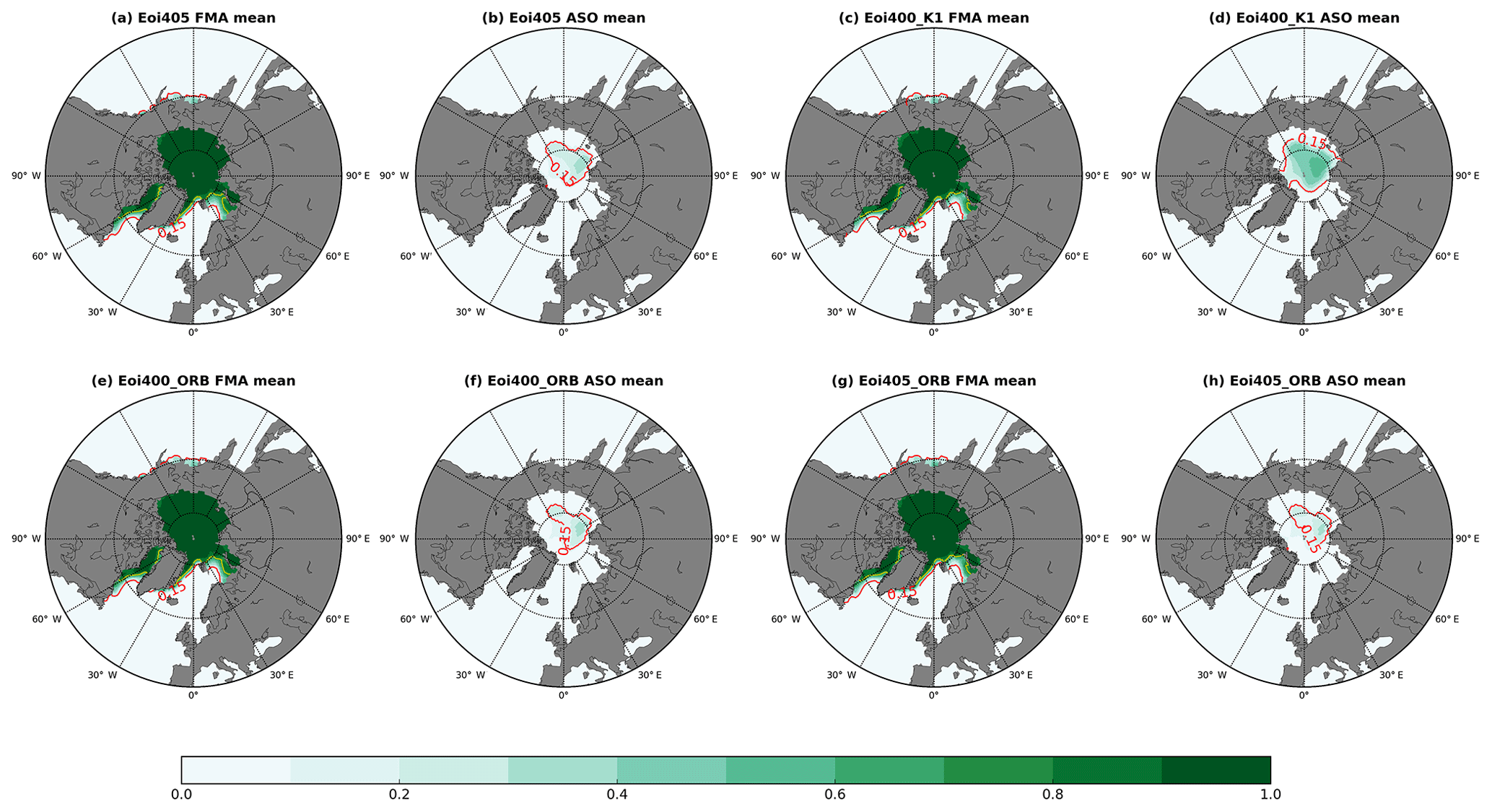
Figure 12 Seasonal mean Arctic sea ice concentration averaged over 100 model years as simulated by COSMOS for mid-Pliocene simulations in response to changes in PlioMIP's prescribed boundary conditions. Panels (a), (c), (e), and (g) show winter (FMA) averages, while panels (b), (d), (f), and (h) show summer (ASO) averages for simulations Eoi405, Eoi400_K1, Eoi400_ORB, and Eoi405_GHG_ORG, respectively. The red contours indicate the 15 % isoline of sea ice cover, while yellow contours indicate the 75 % isoline of sea ice cover.

3.3 Effect of alternative orbit (MIS K1) on mid-Pliocene simulations

Analyzing the effect of a different orbital configuration that is known to have been present during the mPWP, we find via a comparison between Eoi400_K1 and Eoi400 that specifying orbital parameters, representative of MIS K1, will produce a mid-Pliocene climate that is warmer at low and high latitudes and in the Arctic but that is colder in the Southern Hemisphere polar region (see Fig. 5). While almost all landmasses are warming in the annual mean under the influence of MIS K1 orbital forcing, cooling is evident over the southern part of the modern United States, northern Greenland, northern Australia, and some parts of Eurasia. With the exception of the impact of eccentricity, orbital forcing causes a redistribution of incoming solar radiation across latitudes and seasons, rather than a change in the overall input of solar radiation into the climate system. Hence, it is of particular interest to study the seasonality of the climatic effect. We find that the impact of MIS K1 orbital forcing is stronger at a seasonal timescale than in the annual mean. We show time-mean SAT anomalies for boreal summer (JJA) and boreal winter (DJF) in order to analyze the orbital control on the seasonality of the mid-Pliocene (Fig. 5b and c). Our finding is that in simulating the mid-Pliocene, the choice of orbit has a great influence on seasonal patterns of SAT. During boreal winter (Fig. 5c), the K1 orbit is warmer with respect to KM5c, with a maximum SAT anomaly of 3.5 ^∘C in comparison to the simulation with the KM5c orbit, while averages over boreal summer months provide a colder Northern Hemisphere for Eoi400_K1. Substantial winter warming is present over Eurasia, North and South America, and southwestern Africa. SAT over Greenland shows pronounced seasonal variation, with warming during winter and cooling in summer. We note potential implications of relative summer cooling for the state of the Greenland Ice Sheet during the mPWP.

With respect to the impact of K1 orbital forcing on mPWP climate in the Southern Hemisphere, we find that the seasonal dependency of the temperature anomaly is different for Antarctica, where cooling is dominant all year. SAT changes in the Southern Hemisphere during summer are not statistically significant in many regions based on the significance test to account for effective degrees of freedom by means of the autocorrelation method of Matalas and Dawdy (1964). This indicates similarity between summer SAT simulated in this region for both K1 and KM5c (see Fig. 5b).

Furthermore, Eoi400_K1 produces warmer Northern Hemisphere oceans than Eoi400, with the few but obvious exceptions being the Arctic Ocean beyond the Barents Sea, Greenland Sea, Hudson Bay, and the central North Pacific Ocean, where (regional) cooling is observed (Fig. 10). The Southern Ocean, on the other hand, shows mixed signals of warming and cooling under the influence of K1 orbital forcing, with the most pronounced SST increase noticed to the southeast of Australia and South America, which is probably related to a shift of the polar fronts, and also between 100^∘ and 160^∘ E off the Antarctic coast (Fig. 10). The North Atlantic pattern is largely similar to that of the difference between Eoi405 and Eoi400 when considering the effect of changes in orbital forcing on mid-Pliocene SSTs (Fig. 9b), with the obvious difference being a modification of the warming–cooling pattern and the decreased magnitude of SST anomalies. Analyzing the influence of MIS K1 orbital forcing on simulated SSTs of the mPWP, we find that a maximum anomaly of 2.2 ^∘C is obtained from the difference between Eoi400_K1 and Eoi400 in the midlatitudes (Fig. 10).

Allowing variation in orbital configuration within the limits of plausibility during the mPWP by comparing the sea ice concentration from Eoi400_K1 with Eoi400 shows a larger sea ice extent and concentration during boreal summer as a result of the K1 orbital configuration (Fig. 12). Enhanced warming in the Northern Hemisphere polar regions during summer is simulated for MIS KM5c (Fig. 10). Hence, colder conditions with increased summer sea ice prevail for K1 (see Fig. 12). Simulation Eoi400 shows a considerable amount of boreal winter sea ice around the pole and a gradual reduction towards the continents, a result that is largely in agreement with Eoi400_K1, with the exception of the Barents Sea where MIS K1 orbital forcing leads to reduced winter sea ice in comparison to the PlioMIP2 reference orbit KM5c (compare Figs. 11g and 12c).

4 Discussion

When comparing large-scale patterns of mPWP climate simulated by us with COSMOS in the framework of PlioMIP1 and PlioMIP2, we find that the mPWP offers a glimpse into a climate state that is overall warmer than the conditions humankind is currently experiencing. It is noteworthy that relative warmth in the mPWP is possible with a prescribed CO₂ forcing that is actually below the current volume mixing ratio in the atmosphere – 400 ppmv in PlioMIP2's mPWP, about 407 ppmv for 2018 (Friedlingstein et al., 2019, and one reference therein). Yet, we also infer that updates of the model setup from PlioMIP1 to PlioMIP2 lead to both a global and a regional modulation of the overall warmth simulated for the mPWP with respect to PI.

One of the main objectives of the PlioMIP is to determine the dominant components of mid-Pliocene warming derived from the imposed boundary conditions (Haywood et al., 2016). For the COSMOS simulation in response to PlioMIP1 boundary conditions (simulation PlioM1), the most pronounced warming is evident over areas where changes in albedo and orography have been implemented (Stepanek and Lohmann, 2012). This is also the case for PlioMIP2 simulations with COSMOS, above all for the PlioMIP2 core simulation Eoi400. However, the increased number of simulations with dedicated sensitivity studies in PlioMIP2, in comparison to the approach in PlioMIP1, which considered only one simulation based on the best knowledge of mPWP boundary conditions (Haywood et al., 2010, 2011), allows a proper inference of the main drivers of mid-Pliocene warmth. While the study by Stepanek et al. (2020) aims at unraveling the various contributions of PRISM4 boundary conditions to the mPWP climate anomaly as simulated with COSMOS, with this study we employ further sensitivity experiments that go beyond the PlioMIP2 modeling protocol in order to determine the relative contribution of updates in the boundary conditions of COSMOS from PlioMIP1 to PlioMIP2. Our aim is to bridge the gap between COSMOS contributions to PlioMIP1 and PlioMIP2, which are based on model setups that differ beyond the differences between boundary conditions outlined in protocols for PlioMIP1 (Haywood et al., 2010, 2011) and PlioMIP2 (Haywood et al., 2016). Our extended modeling approach allows inference into the contributions of different components to the results achieved with COSMOS in PlioMIP2. Our respective inferences are outlined below.

Generally, we find that the effects of changes in boundary conditions are pronounced in the higher latitudes, while SAT and SST are largely unchanged in the lower latitudes. Hence, for COSMOS the impact of updates of the modeling methodology from PlioMIP1 to PlioMIP2 (encompassing the implementation of PRISM4 boundary conditions with slightly reduced CO₂, increased detail of the mPWP land–sea mask and gateway configuration, and the resolution of climate–vegetation feedbacks via the use of the model's dynamic vegetation module) modifies the polar amplification in the simulated mPWP climate. While regionally the PlioMIP2 core simulation Eoi400 is warmer than the respective climate state of PlioMIP1 (simulation PlioM1), in particular where the ice sheet reconstruction is updated in PRISM4 and regionally in the North Atlantic, the Arctic is generally cooler in our contribution to PlioMIP2. A lower-temperature anomaly in the Arctic imprints on sea ice conditions in high latitudes of the Northern Hemisphere and the global average temperature simulated in PlioMIP2, whereby a small reduction of the modeled temperature anomaly is evident from PlioMIP1 to PlioMIP2. Generally, we find that, in relation to updated gateways, there is a pronounced regional increase in SST in the North Atlantic Ocean, while reduced carbon dioxide leads, as expected, to an overall cooling of the mPWP climate in COSMOS simulations of PlioMIP2. Yet, a comparison of SAT simulated in the framework of a sensitivity study, wherein the PlioMIP2 core simulation Eoi400 is repeated with the higher CO₂ forcing employed in PlioMIP1 simulation PlioM1, reveals that the impact of radiative forcing by increased CO₂ is hemispherically dependent. In the PlioMIP2 model setup with increased CO₂ (as in PlioMIP1), the North Atlantic and large parts of the Mediterranean and Arctic are actually cooler than in the standard PlioMIP2 model setup with 400 ppmv CO₂. In contrast, for the Southern Hemisphere, North Atlantic equatorward of 30^∘ N, and most of the North Pacific, a model setup with the higher PlioMIP1 CO₂ forcing would indeed lead to a warmer mPWP state than what is simulated in our PlioMIP2 core simulation Eoi400. Our CO₂ sensitivity study within the framework of PlioMIP1 and PlioMIP2 shows that a difference of 5 ppmv between the two phases of PlioMIP causes appreciable changes in SAT over land and oceans. The increase in CO₂ produces warmer oceans in the PRISM4-based model setup, except for parts of the North Atlantic and the Arctic as outlined above. As in the PRISM4 COSMOS model setup the effect of increased CO₂ is opposite to the pronounced mPWP warming simulated in the North Atlantic that is found in PlioMIP2 simulation Eoi400 in comparison to PlioMIP1 simulation PlioM1; we conclude that the warmer North Atlantic simulated by us in PlioMIP2 is not influenced so much by changes in greenhouse forcing as it is by the collective contribution of all boundary conditions, in particular the reconfiguration of gateways. As a matter of fact, considering the magnitude of the effect that relatively small changes in CO₂ have in the PlioMIP2 mPWP setup of COSMOS on the temperature of the North Atlantic Ocean leads us to the inference that the gateway effect on North Atlantic Ocean warmth is modulated in our model by greenhouse forcing and that our PlioMIP2 model setup does not provide a final statement with regard to the strength of the gateway effect that may have impacted the mPWP temperature signals interpreted from the geologic recorder. This is either due to longwave oceanic variability or strong internal variability within the model. Hence, averaging over a longer time period greatly reduces the cold anomaly over the North Atlantic (Fig. S2 in the Supplement), and we suggest that this points rather to internal variability in the model as a cause for the cold blob. Other model configurations with altered greenhouse gas forcing may well produce a larger temperature anomaly than the COSMOS PlioMIP2 core simulation Eoi400. If we extend our focus beyond model performance within PlioMIP2, then we find that a PlioMIP2 COSMOS simulation with the higher volume mixing ratio of 405 ppmv of CO₂ is actually in better agreement with the PlioMIP1 simulation PlioM1 in parts of the North Atlantic Ocean (where that simulation suggests colder SST than the PlioMIP2 core simulation Eoi400). Consequently, our results show that a slightly higher CO₂ forcing provides larger disagreement between modeled and reconstructed SST, as both model setups of PlioMIP1 and PlioMIP2 are, in comparison with temperature data derived from proxy records, too cold.

Changes in modern-day orbital forcing between COSMOS PlioMIP1 and PlioMIP2 model setups and the corresponding mid-Pliocene simulations overall promote polar amplification in the former, with the exception of midlatitude to high-latitude continental regions and parts of the North Atlantic Ocean (Fig. 4b). In particular, parts of the central Arctic are slightly cooler with the updated orbital forcing in PlioMIP2, while parts of the North Atlantic Ocean are warmer. Beyond the impact of details of the modern-like PI orbital forcing in our PlioMIP model setups, orbital forcing can play a major role in achieving warmer or colder simulated mid-Pliocene conditions. It can lead to significant annual and seasonal variations (Prescott et al., 2014). Therefore, prescribing modern-day orbital parameters for a mid-Pliocene simulation, and comparing the results with proxy data averaged over multiple time slices within the mid-Pliocene, could increase the cases of data and model discord (Dowsett et al., 2013). Sensitivity tests of PlioMIP1 ensemble models, reported by Salzmann et al. (2013), identified insufficient temporal constraints hampering the accurate configuration of model boundary conditions as an important factor impacting data–model discrepancies. Prior to the start of PlioMIP2, a more defined orbital time slice was suggested to allow a robust evaluation of present climate models to predict warm climates (Prescott et al., 2014). Thus, within the framework of PlioMIP2, a more defined orbital time slice (MIS KM5c) has been specified (Haywood et al., 2016). Even though it reflects a clear signature of MIS KM5c when compared with K1 in the North Atlantic, reconstructions which are available for comparison still reflect signals of multiple time slices within the mid-Pliocene. This could lead to increased cases of model–data mismatch, as our results demonstrate pronounced annual and seasonal variation in SATs and SSTs between two different orbital time slices (K1 and KM5c) of the mid-Pliocene, although with a more pronounced signature of the KM5c climate state. With the increasing availability of SST reconstructions for time slices within the mid-Pliocene period, we also compared with the alkenone-based (${\mathrm{U}}_{\mathrm{37}}^K$) reconstruction of Foley and Dowsett (2019), which refers to time windows of 10 kyr and 30 kyr before present, based on PlioVAR synthesis and the new BAYSPLINE calibration, as well as the magnesium-to-calcium ratio (Mg ∕ Ca) based on PlioVAR synthesis and the new BAYMAG calibration by McClymont et al. (2020). The result shows that the PlioMIP2 simulation in COSMOS agrees best with the ${\mathrm{U}}_{\mathrm{37}}^K$ BAYSPLINE reconstruction in the North Atlantic.

We also find that mid-Pliocene orography and ocean gateways contribute more relative to the location where they are applied. Due to a reduction in ice sheet extent, orography over Greenland was lower by more than 1500 m during the mid-Pliocene relative to the present day (Yan et al., 2013). The COSMOS mid-Pliocene simulation with PlioMIP1 boundary conditions shows that warming related to elevation reduction implied by the reconstructed lower-than-present Greenland Ice Sheet contributes about 80 % of the total warming at this location when compared with the PI (Stepanek and Lohmann, 2012). Assuming a lapse rate of 6.5 K per elevation change of 1000 m, the PlioMIP2 mid-Pliocene core simulation shows that orography contributes 75 % to the mid-Pliocene warming over Greenland with respect to the prescribed PI simulation.

The PlioMIP1 model ensemble showed a diverse picture of mid-Pliocene AMOC with respect to PI. Only a slight increase in meridional ocean heat transport was found by a small number of models. A consistent increase in AMOC and the related meridional ocean heat transport is lacking in the PlioMIP1 model ensemble (Z.-S. Zhang et al., 2013). Even in the COSMOS model, wherein both AMOC and meridional heat transport are slightly enhanced in PlioMIP1, the simulated warming in the North Atlantic Ocean does not reproduce the relative warmth indicated by the available mid-Pliocene SST reconstruction by Dowsett et al. (2013). In an attempt to simulate enhanced mid-Pliocene AMOC, studies have suggested that closure of the Bering Strait would lead to enhanced AMOC (Hu et al., 2015). Furthermore, it has been stated that the modification of certain seafloor features could increase the strength of AMOC (Brierley and Fedorov, 2016; Robinson et al., 2011). With respect to the SST of the mPWP, Otto-Bliesner et al. (2016) have explored the climatic effect of adjustments of the Bering Strait, Canadian Arctic Archipelago, and Hudson Bay towards their respective states during the Pliocene. With changes in prescribed geography for PlioMIP2 mPWP simulations that incorporate the assumed modifications of ocean gateways in the mPWP with respect to modern, we find that COSMOS indeed simulates an enhanced AMOC for PlioMIP2 with respect to PlioMIP1. Enhanced AMOC also relates in COSMOS to a warmer North Atlantic surface ocean in the PlioMIP2 simulation Eoi400. Consequently, the PlioMIP2 mPWP simulation with adjusted (i.e., closed) Bering Strait reduces the model–data mismatch found by Dowsett et al. (2013). With regards to variations of the PI orbital configuration, we note that the extremely small amplitude of the variation of the orbital forcing suggests that at least a part of the SST effect that we derive from the simulations is caused by internal variability in the climate system rather than an imprint of the modified model setup. Although large parts of the anomaly are found to be statistically significant, we cannot exclude the possibility that a part of the simulated SST pattern is not a stable climate feature, but rather an overprint of slow modes of climate variability, whose periodicity is beyond the analysis period of 100 model years.

From our SAT analyses, we find that PRISM4 paleogeography seems to be the dominant factor driving the mid-Pliocene warmth. This is shown by comparing the mid-Pliocene simulation with PRISM4 paleogeography Eoi405_ORB to the PlioM1 coupled ocean–atmosphere experiment, with the result that the same SAT patterns emerge as generated by the total effect of switching from the PlioMIP1 to PlioMIP2 setup (derived from the comparison PlioM1 vs. Eoi400). Similar analysis for SST (Fig. 9) shows that PRISM4 paleogeography is not the only factor producing a warmer North Atlantic, but the combined effect of PlioMIP2 boundary conditions. Donnadieu et al. (2006) demonstrate that land and ocean climates are affected differently by changes in paleogeography. Within the framework of PlioMIP2, PRISM4 paleogeography prevents fresher seawater from the Pacific from reaching the North Atlantic via the Arctic due to the closure of the Bering Strait, having a significant influence on SSTs in this region.

If we turn to the effect of alternative mPWP forcing on climate simulated in COSMOS, then seasonal analysis of our simulations shows that sea ice and SST are not only sensitive to prescribed CO₂. Orbital forcing and the state of imposed paleogeography can also influence the simulated sea ice extent and concentration. A reduced spatial extent is evident, in particular during boreal summer, for simulations with the KM5c orbit with respect to simulations that are forced by K1 orbit. Simulations with orbital configurations of K1 show colder high latitudes in summer, as well as warmer middle to high latitudes, and thus impact simulated sea ice in the Arctic. This is attributed to high eccentricity estimated for K1, leading to a more elliptical orbit around the sun, which in turn affects the distribution of insolation for different seasons (Fischer and Jungclaus, 2011). While the COSMOS PlioMIP1 simulation PlioM1 shows close to ice-free conditions in the Arctic during boreal summer, PlioMIP2 core simulation Eoi400 is characterized by relatively increased summer sea ice conditions in the Arctic Ocean, although sea ice cover in this simulation is still low in comparison to, for example, the PI control state PI_2. Our exercise in considering alternative orbital configurations that are equally as plausible for the mPWP as the reference orbit KM5c reveals that we can create with COSMOS a third realization of mPWP Arctic summer sea ice that differs from both the PlioMIP1 and PlioMIP2 COSMOS mPWP sea ice states. Although overall the K1 orbit provides larger total incoming solar shortwave radiation than the Earth receives during modern times (Prescott et al., 2014), under its influence Arctic summer sea ice is enhanced in comparison to the PlioMIP2 core simulation. This effect is even stronger with respect to the mPWP state simulated with COSMOS in PlioMIP1. These findings highlight the degree of variability that is present in the simulation of Arctic Ocean sea ice conditions across the mPWP – even if only one climate model is considered that is exposed only to those modifications of boundary conditions that are considered to be within the range of possibility during the mPWP. Consequently, the variability of Arctic sea ice in our study reminds us of the temporal variability that sea ice may have been subject to across the Pliocene epoch. The variability of Arctic sea ice, more precisely its temporal evolution, has been linked to the development of the Greenland Ice Sheet (Clotten et al., 2019). Therefore, we highlight the scientific merit that may arise from studying both the inter-model and time variability of Arctic sea ice across the mPWP. This may be done, for example, in the framework of upcoming iterations of PlioMIP and may lead us towards a better understanding of the climate transition from the Cenozoic “greenhouse” to the Pleistocene “icehouse”. We highlight that fact that the study of the inter-model variability of sea ice evolution, in particular across multiple orbital configurations during mPWP, which is beyond the framework of our publication, should be pursued in future work. While simulations of MIS KM5c employ the orbital configuration of the present day, which has been demonstrated to simulate an ice-free summer for the mid-Pliocene, there is an appreciable degree of inter-model spread that is at a similar amplitude as uncertainty in proxy-based reconstructions of mPWP Arctic sea ice extent (Howell et al., 2016). Variability in simulated sea ice extent and thickness within the PlioMIP1 ensemble is reported to be the effect of differences in the sea ice components of each model (Howell et al., 2016).

We conclude our discussion by noting that the results of this study suggest that there is an appreciable amplitude of internal variability inherent in mPWP climate simulations produced with COSMOS – this is also potentially the case for other models, which could be tested in the future. One of our findings is that relatively small variations of the prescribed climate forcings, which are represented in our study by variations of greenhouse gas concentrations of the order of a few parts per million by volume of CO₂, and very minor modifications of an otherwise PI orbital configuration can lead to localized, but non-negligible, mPWP climate anomalies. While we did not explicitly study the reasons behind this finding, the small amplitude of the overall forcing anomaly suggests that the linked variation of the mPWP climate anomaly, computed over a time period of 100 model years, is likely at least partly a result of the modulation of internal variability in the model that is triggered by alteration of the model forcing. While PlioMIP2 already made a major leap forward by increasing the analysis time period from 30 years in PlioMIP1 to 100 years in PlioMIP2, this finding highlights the fact that in future intercomparisons it may be worthwhile to further increase the analysis time period towards multicentennial timescales. Our suggestion is motivated by the observation that beyond the common short-term climate variability that occurs, for example, in the form of the El Niño–Southern Oscillation (Christensen et al., 2013, see their Fig. 14.13) and North Atlantic Oscillation (Hurrell, 1995, see their Fig. 1A), there are certain modes of internal variability that act at ocean basin scale with a much larger recurrence time. If the PlioMIP analysis period were at multicentennial timescales, such slow modes of internal variability would be more likely suppressed by averaging over multiple realizations of climate patterns that are related to opposite phases of these modes, hence leading to a clearer emergence of a mean (predominant across time periods of centuries) mPWP climate state.

5 Summary and conclusions

In this study, we compared the results of mid-Pliocene simulations within the frameworks of PlioMIP1 and PlioMIP2 that have been carried out with COSMOS at the Alfred Wegener Institute in Germany. We have tested to what degree changes between the COSMOS model setups of PlioMIP1 and PlioMIP2 are able to create different realizations of simulated mPWP climate and how different these alternative mPWP climate states are from PlioMIP2 core simulations Eoi400 and PlioM1, both produced with the same climate model as employed in this study. Overall, we find that the global patterns of mPWP climate, as expressed in SST and SAT, are similar in PlioMIP2 and PlioMIP1. Yet, in PlioMIP2 we simulate certain differences that impact, in particular, sea ice conditions in the Arctic and the amplitude of the mPWP temperature anomaly in the North Atlantic Ocean. Beyond small changes in the PI orbit reference configuration in COSMOS and the modification of CO₂ that arises from the transition of PRISM3D to PRISM4 boundary conditions, we carried out sensitivity experiments that address the climatic impact of plausible orbital configurations across the mPWP (MIS KM5c and K1) to assess variability across different discrete time slices within the mid-Pliocene warm period using boundary conditions prescribed for PlioMIP2.

From our results, we conclude that paleogeography is the dominant component of the imposed mid-Pliocene boundary conditions, influencing the climate across the warm period. Its effect on the atmosphere and ocean differs as seen in the different pattern of warming and cooling achieved for SAT and SST. We also conclude that the response of atmospheric and oceanic variables differs distinctly when exposed to the same geography. The 5 ppmv difference in CO₂ between PlioMIP1 and PlioMIP2 simulations does not change the general impression of large-scale mPWP climate patterns but samples the strong internal model variability; thus, PlioMIP1 and PlioMIP2 simulations are mostly impacted by changes in paleogeography from PRISM3 to PRISM4. The impact of a small amplitude of change in orbital forcing leads us to the suggestion that the simulated PlioMIP climate state may be subject to appreciable internal variability that, while not changing the overall impression of the characteristics of simulated mPWP climate, provides regional patterns of SST and SAT that are worthwhile to study in future phases of PlioMIP based on a prolonged multicentennial analysis period.

Furthermore, the newly prescribed PlioMIP2 boundary conditions play a significant role in achieving warmer North Atlantic SSTs that were modeled too cold during PlioMIP1 if compared to reconstructions. On the other hand, the PlioMIP2 mPWP reference state simulated with COSMOS (simulation Eoi400) is globally slightly cooler, in agreement with reduced concentrations of CO₂, and also expresses itself via reduced warmth and resultantly increased summer sea ice conditions in the Arctic Ocean. When considering various modifications of mPWP boundary conditions in our simulations, we find that there is the potential for pronounced variability of Arctic summer sea ice conditions during the mPWP. Enhanced AMOC in PlioMIP2 is achieved through the combined effect of PlioMIP2 boundary conditions, contributing to the increased meridional transport of warm water from low to midlatitudes in the North Atlantic. We note that details of the model forcing, in particular the exact level of carbon dioxide and the realization of the KM5c orbit surrogate, have an impact on the amplitude of North Atlantic Ocean warming in comparison to results derived with COSMOS in PlioMIP1. With respect to PI conditions, an extended equatorial warm pool, shown in COSMOS simulation PlioM1 for PlioMIP1, is also present in our PlioMIP2 simulation Eoi400 with a similar spatial pattern and extent. This is in line with our finding that the effect of changes in mid-Pliocene boundary conditions from PlioMIP1 to PlioMIP2 is minor in low latitudes and more pronounced in high-latitudes. The magnitude of Arctic warming simulated for PlioMIP1 is reduced in our PlioMIP2 simulation, while increased warming over Greenland and Antarctica is a direct effect of changes in reconstructed orography and albedo from PlioMIP1 to PlioMIP2.

Employing a different plausible mPWP orbital forcing (MIS K1) in simulating the mid-Pliocene, and comparing the results to those derived based on the standard PI orbital configuration that is used as a surrogate for the MIS KM5c, reveals pronounced climate anomalies that may express themselves via both warming and cooling at various spatial scales – the former mostly at high latitudes, in particular in the Arctic Ocean, and the latter widespread in low to midlatitudes. Comparison between climate states simulated for both the KM5c and K1 time slices shows annual and seasonal variations, with the RMSD between the modeled North Atlantic SSTs for these time slices on one side and the reconstructions of mPWP SSTs on the other side showing better agreement between the geologic record and the simulation for MIS KM5c (Eoi400) in contrast to MIS K1. This confirms a more pronounced signal of the KM5c climate state in the reconstruction. Yet, in line with statements by previous authors (Dowsett et al., 2016; Haywood et al., 2016; Prescott et al., 2014; Salzmann et al., 2013), further steps should be taken to reconstruct the mid-Pliocene climate within the KM5c time slice, as this will reduce signals and interferences that could be caused by averaging over multiple isotope excursion periods when comparing with modeled data.